A general multiblock method for structured variable selection

The structured penalties, $\Omega_{k}$, considered in this paper are convex but possibly non-differentiable. The functions $\Omega_{k}$ must fit the framework of Nesterov, as described in [8], and will be written in the form

in which $\mathcal{G}_{k}$ is the number of groups for the particular function $\Omega_{k}$. A group constitutes the variables with associated non-zero entries in $\mathbf{A}_{k,G}$ (this would be e.g. the pixels or voxels associated with the gradient at a particular point in total variation, or a group of related variables in group $\ell_{1,q}$). The group matrix $\mathbf{A}_{k,G}$ is a linear operator for group $G$ associated with the function $\Omega_{k}$, for $k=1,\ldots,K$. The function $\|\cdot\|_{q}$ is the standard $\ell_{q}$-norm defined on $\mathbb{R}^{p}$ by $\|\mathbf{x}\|_{q}=\sqrt[q]{\sum_{j=1}^{p}|x_{j}|^{q}}$, with the associated dual norm $\|\cdot\|_{q^{\prime}}$ for $q,q^{\prime}\geq 1$. Nesterov’s smoothing technique [8, 11] is formally defined as follows.

When smoothing the functions $\widehat{\Omega}_{k}$ this way, we obtain

An immediate consequence is that since the functions $\widehat{\Omega}_{k}$ are convex and differentiable they may, for a sufficiently small value of $\mu_{k}$, be used instead of $\Omega_{k}$.

The gradients of the Nesterov smoothed functions, $\widehat{\Omega}_{k}(\mu_{k},\mathbf{w}_{k})$, with respect to the corresponding $\mathbf{w}_{k}$ are

The gradients are Lipschitz continuous with Lipschitz constant

where $\|\mathbf{A}_{k}\|_{2}$ is the spectral norm of $\mathbf{A}_{k}$.

Nesterov’s smoothing technique allow us to have a smooth objective function with convex constraints. In order to find a minimiser to Equation 2.4 we must first alter the formulation slightly.

The constraints are rephrased as follows: We construct the sets $\mathcal{P}_{k}$ and $\mathcal{S}_{k}$ as $\mathcal{P}_{k}=\{\mathbf{x}\in\mathbb{R}^{p_{k}}\;|\;\|\mathbf{x}\|_{1}\leq s_{k}\}$ and $\mathcal{S}_{k}=\{\mathbf{x}\in\mathbb{R}^{p_{k}}\;|\;\mathbf{w}_{k}^{\mathrm{T}}\mathbf{M}_{k}\mathbf{w}_{k}\leq 1\}$, and then form the intersection set, $\mathcal{W}_{k}=\left\{\mathbf{x}\;|\;\mathbf{x}\in\mathcal{P}_{k}\cap\mathcal{S}_{k}\right\}$. Therefore, we are interested in block weight vectors $\mathbf{w}_{k}$ such that $\mathbf{w}_{k}\in\mathcal{W}_{k}$. We will suppose that $\mathcal{W}_{k}\neq\emptyset$ and in fact assume that at least $\mathbf{0}\in\mathcal{W}_{k}$. We note that all $\mathcal{W}_{k}$ are convex sets, since $\mathcal{P}_{k}$ and $\mathcal{S}_{k}$ are convex sets.

The optimisation problem in Equation 2.4, and the final optimisation problem that we will consider in this paper, can thus be stated as

This single indicative constraint for each block is equivalent to the constraints in Equation 2.4. When $\mu_{k}\rightarrow 0$, the two problems in Equation 2.4 and Equation 2.6 are equivalent.

The partial gradients of the objective function in Equation 2.6 with respect to each $\mathbf{w}_{k}$ are

for all $k=1,\ldots,K$, where we let $\text{Cov}(\mathbf{X}_{k}\mathbf{w}_{k},\,\mathbf{X}_{j}\mathbf{w}_{j})=\frac{1}{n-1}\mathbf{w}_{k}^{\mathrm{T}}\mathbf{X}_{k}^{\mathrm{T}}\mathbf{X}_{j}\mathbf{w}_{j}$, i.e. the unbiased sample covariance.

We see in Algorithm 2 that orthogonal projections onto the convex sets $\mathcal{W}_{k}$ are required at each iteration of the algorithm, and for each block.

The projection onto the intersection of two convex sets, $\mathcal{W}=\mathcal{P}\cap\mathcal{S}$, is formulated as the unique point that minimises the problem

where $\iota_{\mathcal{W}_{k}}$ is the indicator function over $\mathcal{W}_{k}$, i.e.

We note that the right-most side of Equation 3.1 is in fact the proximal operator of the indicator function over the set $\mathcal{W}_{k}$, and thus that the proximal operator of the indicator function is the projection onto the corresponding set.

The projection onto the intersection $\mathcal{P}\cap\mathcal{S}$ can be computed using Dykstra’s projection algorithm [5], stated in Algorithm 1. The sequence $(\mathbf{x}^{(s)})_{s\in\mathbb{N}}$ generated by Algorithm 1 converges to the unique point that is the solution to Equation 3.1.

We thus use Algorithm 1 to find the projection onto the intersection of the two sets $\mathcal{P}$ and $\mathcal{S}$. This is necessary in order to enforce the constraint in Equation 2.6. Three key points need to be explained in order to make Algorithm 1 clear:

1. (i)

   the projection onto $\mathcal{P}$ (Line 3),

2. (ii)

   the projection onto $\mathcal{S}$ (Line 5), and

3. (iii)

   the stopping criterion (Line 7).

These points are discussed in the following subsections.

We are now ready to discuss the full multiblock accelerated projected gradient method, a generalised RGCCA minimisation algorithm. This algorithm is presented in Algorithm 2.

Any appropriate minimisation algorithm can be used in the inner-most loop of Algorithm 2. We use the fast iterative shrinkage-thresholding algorithm (FISTA) [1, 2], since it has the optimal (for first-order methods) convergence rate of $\mathcal{O}(1/s^{2})$, where $s$ is the iteration count.

FISTA requires a step size, $t_{k}$, for each block and each step of the iterative algorithm, as seen on Line 6 of Algorithm 2. If all partial gradients of the objective function in Equation 2.6, i.e. the gradients in Equation 2.7, are Lipschitz continuous, then we can compute the step size directly. In that case, the step sizes, $t_{k}$, are computed as the reciprocal of the sum of the Lipschitz constants of the gradients, as explained in [8]. I.e., such that

where $\mu_{k}$ is the parameter for the Nesterov smoothing; the partial gradients are from the the loss function in Equation 2.6, i.e. the Lipschitz constants of the partial gradients in Equation 2.7. If some gradient is not Lipschitz continuous, or if the sum of Lipschitz constants would be zero, the step size can also be found efficiently by using backtracking line search.

Note that the main stopping criterion on Line 13 is actually performing a step of the iterative soft-thresholding algorithm (ISTA). This stopping criterion can easily be explained as follows: Assume a function on the form

where $g$ is smooth and convex, and $h$ is convex, but non-smooth, and whose proximal operator is known. We recall and rewrite the ISTA descent step,

where

Thus, it is clear that convergence has been achieved if $G_{t}(\mathbf{x}^{(s)})$ is small. In fact, it follows from the definition of subgradients and the optimality condition of proximal operators [14] that

and that $G_{t}(\mathbf{x})=\mathbf{0}$ if and only if $\mathbf{x}$ minimises $f(\mathbf{x})=g(\mathbf{x})+h(\mathbf{x})$.

We illustrate the proposed method by predicting the location of brain tumours from GE and CGH data [13]. The problem is one with three blocks: GE ($\mathbf{X}_{1}\in\mathbb{R}^{53\times 15702}$), CGH ($\mathbf{X}_{2}\in\mathbb{R}^{53\times 41996}$) and a dummy matrix encoding the locations ($\mathbf{X}_{3}\in\mathbb{R}^{53\times 3}$). The locations were: The brain stem (DIPG), central nuclei (Midline) and supratentorial (Hemisphere).

The purpose of this example is to show the versatility of the proposed method, and to show how it can be used to build an RGCCA model with both complex penalties and sparsity-inducing constraints, and analyse data related to the data used in [19].

The relation design was, the between-block connections, were chosen to be oriented towards prediction, and is illustrated in Figure 1. Therefore, $\mathbf{X}_{1}$ and $\mathbf{X}_{2}$ are connected to $\mathbf{X}_{3}$ ($c_{13}=c_{23}=1)$, but there is no connection between $\mathbf{X}_{1}$ and $\mathbf{X}_{2}$ (i.e., $c_{12}=0$). This design tends to focus on models where prediction can be made even if there is no relation between the predictor blocks, and in [19] it was indeed the case on equivalent data that this design yielded the best prediction rates among similar designs.

An $\ell_{1}$ and a group $\ell_{1,2}$ [18, 14] constraint were added to the GE block, $\mathbf{X}_{1}$. An $\ell_{1}$ together with a total variation [10], constraint were added to the CGH, $\mathbf{X}_{2}$, block in order to smooth the often noisy CGH data.

The regularisation constants, $\tau_{k}$, for $k=1,2,3$, were computed using the method of Schäfer and Strimmer [16], and were $\tau_{1}=1.0$ and $\tau_{3}=1.0$, for blocks $\mathbf{X}_{1}$ and $\mathbf{X}_{3}$, respectively. For $\mathbf{X}_{2}$ we were unable to compute the regularisation constant, because of the large size of the data. We therefore instead used the mean of ten regularisation constants, computed from random samples of $41\,996/2=20\,998$ variables each, and rounded to one decimal point. The computed mean was $\tau_{2}=0.2623\ldots\approx 0.3$.

The other constants were found by grid search with 7-fold cross-validation. The cross-validation procedure maximised the statistic

in order to force a high prediction rate from both $\mathbf{X}_{1}$ and $\mathbf{X}_{2}$. I.e., $\mathrm{R^{2}_{pred,\mathbf{X}_{3}}}$ is the combined prediction rate from the models of $\mathbf{X}_{1}$ and $\mathbf{X}_{2}$, where the product forces both blocks to predict $\mathbf{X}_{3}$ well. By $\widehat{\mathbf{X}}_{1\rightarrow 3}$ we denote the prediction of the locations, encoded in the dummy matrix $\mathbf{X}_{3}$, from the model of $\mathbf{X}_{1}$ and by $\widehat{\mathbf{X}}_{2\rightarrow 3}$ we denote the prediction of $\mathbf{X}_{3}$ from the model of $\mathbf{X}_{2}$. The $\|\cdot\|^{2}_{F}$ denotes the squared Frobenius norm.

The predictions were computed in the traditional way using the inner (or structural) relation [21, 15, 24], i.e. that the assumed relation between corresponding latent variables is linear,

where

is a regression coefficient. Multiple regression is performed when there are several latent variables.

Finally, we predict with

where $\mathbf{T}_{k}=[\mathbf{X}_{k}\mathbf{w}_{k,1}|\mathbf{X}_{k}\mathbf{w}_{k,2}|\cdots|\mathbf{X}_{k}\mathbf{w}_{k,A}]$ are the $A$ latent variables for block $k$ and $\mathbf{W}_{3}=[\mathbf{w}_{3,1}|\cdots|\mathbf{w}_{3,A}]$ are the $A$ weight vectors for block 3.

The criterion of the final model, as found by the grid search, was

These numbers were computed as the means of 7-fold cross-validation.

The regularisation constant for the group $\ell_{1,2}$ penalty was thus deemed by the grid search to be $\omega_{1}=0.35$ and the $\ell_{1}$ norm constraint had a radius of $s_{1}=13$. The regularisation constant for total variation was $\omega_{2}=0.004$, and the $\ell_{1}$ norm constraint had a radius of $s_{2}=10.1$.

The optimisation problem that we considered in this example was thus

in which $\mu_{1}=\mu_{2}=5\cdot 10^{-4}$. Two components were extracted using the deflation scheme [19]

In order to illustrate one of the main benefits of the proposed method, we performed a simulation study in which we compared the differences between the weight vectors of the proposed method and “regular” unpenalised RGCCA to the weight vectors used when generating the simulated data.

We generated data for two blocks, $\mathbf{X}_{1}\in\mathbb{R}^{50\times 150}$ and $\mathbf{X}_{2}\in\mathbb{R}^{50\times 100}$, defined by the models

where $\mathbf{t}_{1}\sim\mathcal{N}(\mathbf{0},\mathbf{I}_{50})$, $\mathbf{t}_{2}\sim\mathcal{N}(\mathbf{t}_{1},0.01^{2}\mathbf{I}_{50})$; the columns of $\mathbf{E}_{1}$, were random normal, $\mathbf{E}_{1,j_{1}}\sim\mathcal{N}(\mathbf{0},0.15^{2}\mathbf{I}_{50})$, and similarly for the columns of $\mathbf{E}_{2}$, such that $\mathbf{E}_{2,j_{2}}\sim\mathcal{N}(\mathbf{0},0.2^{2}\mathbf{I}_{50})$.

We then built an RGCCA model using Equation 2.1 and a regularised RGCCA model using Equation 2.6. The regularised RGCCA model had a total variation penalty and an $\ell_{1}$ constraint for $\mathbf{X}_{1}$, and a group $\ell_{1,2}$ penalty for $\mathbf{X}_{2}$. The block $\mathbf{X}_{2}$ was not given an $\ell_{1}$ constraint in order to illustrate the variable selection that the group $\ell_{1,2}$ penalty provides.

The groups of the group $\ell_{1,2}$ penalty were: $\mathrm{Group~1}=[1,\ldots,10]$, $\mathrm{Group~2}$ $=[11,\ldots,30]$, $\mathrm{Group~3}=[21,\ldots,40]$, $\mathrm{Group~4}=[41,\ldots,60]$, $\mathrm{Group~5}=[61,\ldots,90]$ and $\mathrm{Group~6}=[91,\ldots,100]$, as illustrated in Figure 2. Note in particular that Group 2 and Group 3 are overlapping.

The regularisation constants, $\tau_{1}$ and $\tau_{2}$, were computed using the method of Schäfer and Strimmer [16], and were $\tau_{1}=0.33$ and $\tau_{3}=0.32$, for the blocks $\mathbf{X}_{1}$ and $\mathbf{X}_{2}$, respectively.

We performed a grid search with cross-validation, as in the previous example, in order to find the regularisation parameters. The constants for the regularised RGCCA model were found to be $\omega_{1}=0.61$, $s_{1}=7.7$ and $\omega_{2}=0.13$.

The optimisation problem that we considered in this example was therefore

in which $\mu_{1}=\mu_{2}=5\cdot 10^{-4}$. We only extracted one component in this example.

The locations were predicted using three approaches: From the GE data, $\mathbf{X}_{1}$, from the CGH data, $\mathbf{X}_{2}$, and from both the GE and the CGH data concatenated, i.e. from $\mathbf{X}_{12}=[\mathbf{X}_{1}\,|\,\mathbf{X}_{2}]$. The GE data, $\mathbf{X}_{1}$, were able to predict $43/53\approx 81~\%$ of the locations correctly; the CGH data, $\mathbf{X}_{2}$, were able to predict $38/53\approx 72~\%$ of the locations correctly; and when simultaneously predicting from both the GE and the CGH data, $50/53\approx 94~\%$ of the locations were correctly identified. These numbers are the means of the 7-folds of cross-validated prediction rates. These prediction rates are similar to or higher than those reported in [19] and in the present case, structure was also imposed on the weight vectors.

We performed 100 bootstrap rounds in order to assess how stable the models were, and in particular whether the models are in agreement or not between bootstrap rounds.

We computed an inter-rater agreement measure: the Fleiss’ $\kappa$ statistic [7], in order to asses the agreement between weight vectors computed from the 100 bootstrap rounds in terms of the selected variables for the two components. The number of times a variable is selected or not selected in the 100 bootstrap rounds is counted and summarised by the Fleiss’ $\kappa$, that thus measures the agreement among the bootstrap samples. The higher the value of $\kappa$, the more stable the method is with respect to sampling; positive values means more stable than what could be expected from chance, and $\kappa=1$ means completely stable (all samples agree entirely).

The models were stable, with all Fleiss’ $\kappa>0$. I.e., the weight vectors computed in the different bootstrap rounds agreed in terms of which variables should be included or not in the model. Fleiss’ $\kappa$ was about $0.61$ for the first component of $\mathbf{X}_{1}$, and $0.35$ for the second component; about $0.28$ for the first component of $\mathbf{X}_{2}$ and $0.07$ for the second component.

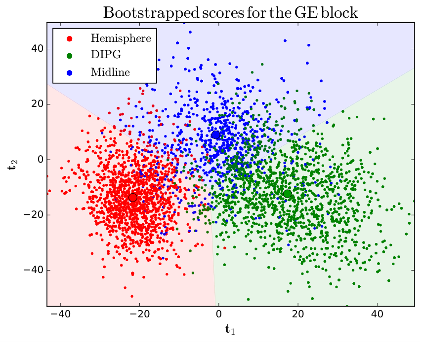
Figure 3 illustrates the first and second components of the models from the samples of the 100 bootstrap rounds; it is clear that the CGH data discriminates the locations very well. The coloured sections are Voronoi regions, and are meant to illustrate the location separation.

Figure 4 illustrates the first and second component of the final RGCCA model for the GE (upper left panel) and CGH (upper right panel) blocks. The lower centre panel illustrates the first components of the GE and CGH blocks plotted against each other. The separation between the locations is clear. It is also clear that the score vectors of the GE and CGH data are correlated, and that the variance of the model of the GE data is higher.

The bootstrap average number of selected variables in $\mathbf{X}_{1}$ was roughly 3 % in both components. In $\mathbf{X}_{2}$, the average number of selected variables was roughly 27 % in the first component, and roughly 40 % in the second component.

The group $\ell_{1,2}$ penalty selected $125.5$ out of the 199 identified groups in the first component and $126.3$ in the second component (these values are bootstrap averages). Groups were considered strong if they had a high ratio between the number of selected gene expressions within the group over the total number of selected gene expressions [4].

Among the top ranking groups were: Alzheimer’s disease (hsa05010), which implies a relation to a supratentorial tumour (in the hemispheres) since it affects the cortex and hypocampus; “Axon guidance” (hsa04360), which implies a relation to DIPG, because of the abundance of axons in the brain stem; and Nucleotide excision repair (hsa03420), since it could explain tendencies towards drug resistance.

Among the groups that were excluded from the model were the Citrate cycle (TCA cycle, hsa00020). Citrate seems to be abundant in DIPG (unpublished results), but its occurrence in other locations is unknown. This would imply that it could be similarly found in the other locations or cancer types as well, and thus be a poor predictor of the tumour locations.

We performed cross-validation in order to find the parameters for the total variation, $\ell_{1}$ and group lasso penalties. The obtained weight vectors were compared to the true ones (those used to generate the data) and to those of an unpenalised, or “regular”, RGCCA model. The weight vectors are illustrated in Figure 5.

The weights from the unpenalised RGCCA model nicely capture the trends in the data, but are affected to a high degree by the noise.

As seen in Figure 5, the weight vectors obtained from the penalised model clearly performs well in reconstructing the true weights; especially so for $\mathbf{X}_{1}$, where the total variation penalty removes much of the noise, but leaves the true weight profile intact. The group lasso penalty manages to remove the groups with true null weights, and appears to find the mean of the other groups.

The weights of $\mathbf{X}_{2}$ that correspond to variable indices 20 through 30 belong to two groups (group 2 and group 3). Those should have weights that are a compromise between describing group 2 and describing group 3. It appears they focus on describing group 2.

References

- [1] Amir Beck and Marc Teboulle. A Fast Iterative Shrinkage-Thresholding Algorithm for Linear Inverse Problems. SIAM Journal on Imaging Sciences, 2(1):183–202, Jan 2009.
- [2] Amir Beck and Marc Teboulle. Gradient-based algorithms with applications to signal recovery problems. In Daniel P. Palomar and Yonina C. Eldar, editors, Convex Optimization in Signal Processing and Communications, chapter 2, pages 42–88. Cambridge University Press, 1 edition, 2009.
- [3] Xi Chen and Han Liu. An Efficient Optimization Algorithm for Structured Sparse CCA, with Applications to eQTL Mapping. Statistics in Biosciences, 4(1):3–26, December 2011.
- [4] Xi Chen, Han Liu, and Jaime G. Carbonell. Structured sparse canonical correlation analysis. volume 22 of JMLR Workshop and Conference Proceedings, pages 199–207, April 2012. AISTATS 2012.
- [5] Patrick L. Combettes and Jean-Christophe Pesquet. Proximal splitting methods in signal processing. In H. H. Bauschke, R. S. Burachik, P. L. Combettes, V. Elser, D. R. Luke, and H. Wolkowicz, editors, Fixed-Point Algorithms for Inverse Problems in Science and Engineering, pages 185–212. New York: Springer, 2011.
- [6] Jan De Leeuw. Block relaxation algorithms in statistics. In H. H. Bock, W. Lenski, and M. M. Richter, editors, Information Systems and Data Analysis, pages 308–325. Springer, Berlin, 1994.
- [7] Joseph L. Fleiss. Measuring nominal scale agreement among many raters. Psychological Bulletin, 76(5):378–382, 1971.
- [8] Fouad Hadj-Selem, Tommy Löfstedt, Vincent Frouin, Vincent Guillemot, and Edouard Duchesnay. An Iterative Smoothing Algorithm for Regression with Structured Sparsity. arXiv:1605.09658 [stat], May 2016.
- [9] Tommy Löfstedt, Fouad Hadj-Selem, Vincent Guillemot, Cathy Philippe, Edouard Duchesnay, Vincent Frouin, and Arthur Tenenhaus. Structured variable selection for regularized generalized canonical correlation analysis. In Hervé Abdi, Vincenzo Esposito Vinzi, Giorgio Russolillo, Gilbert Saporta, and Laura Trinchera, editors, The Multiple Facets of Partial Least Squares Methods, volume 173 of Springer Proceedings in Mathematics & Statistics. Springer, 2016.
- [10] Vincent Michel, Alexandre Gramfort, Gaël Varoquaux, Evelyn Eger, and Bertrand Thirion. Total Variation Regularization for fMRI-Based Prediction of Behavior. IEEE Transactions on Medical Imaging, 30(7):1328–1340, 2011.
- [11] Yurii Nesterov. Smooth minimization of non-smooth functions. Mathematical Programming, 103(1):127–152, December 2004.
- [12] Neal Parikh and Stephen Boyd. Proximal Algorithms. Foundations and Trends in Optimization. Now Publishers Inc., 1st edition, 2013.
- [13] Cathy Philippe, Stephanie Puget, Dorine A Bax, Bastien Job, Pascale Varlet, Marie-Pierre Junier, Felipe Andreiuolo, Dina Carvalho, Ricardo Reis, Lea Guerrini-Rousseau, Thomas Roujeau, Philippe Dessen, Catherine Richon, Vladimir Lazar, Gwenael Le Teuff, Christian Sainte-Rose, Birgit Geoerger, Gilles Vassal, Chris Jones, and Jacques Grill. Mesenchymal transition and PDGFRA amplification/mutation are key distinct oncogenic events in pediatric diffuse intrinsic pontine gliomas. PloS one, 7(2):e30313, January 2012.
- [14] Zhiwei Qin, Katya Scheinberg, and Donald Goldfarb. Efficient block-coordinate descent algorithms for the Group Lasso. Mathematical Programming Computation, 5(2):143–169, Mar 2013.
- [15] Gaston Sanchez. PLS Path Modeling with R. http://www.gastonsanchez.com/PLS_Path_Modeling_with_R.pdf, 2013.
- [16] Juliane Schäfer and Korbinian Strimmer. A shrinkage approach to large-scale covariance matrix estimation and implications for functional genomics. Statistical applications in genetics and molecular biology, 4(1), 2005.
- [17] Mark Schmidt, Nicolas Le Roux, and Francis Bach. Convergence rates of inexact proximal-gradient methods for convex optimization. arXiv:1109.2415, September 2011.
- [18] Matt Silver and Giovanni Montana. Fast identification of biological pathways associated with a quantitative trait using group lasso with overlaps. Statistical applications in genetics and molecular biology, 11(1):Article 7, January 2012.
- [19] Arthur Tenenhaus, Cathy Philippe, Vincent Guillemot, Kim-Anh Lê Cao, Jacques Grill, and Vincent Frouin. Variable Selection For Generalized Canonical Correlation Analysis. 2014.
- [20] Arthur Tenenhaus and Michel Tenenhaus. Regularized Generalized Canonical Correlation Analysis. Psychometrika, 76(2):257–284, 2011.
- [21] Michel Tenenhaus, Vincenzo Esposito Vinzi, Yves-Marie Chatelin, and Carlo Lauro. PLS path modeling. Computational Statistics & Data Analysis, 48:159–205, 2005.
- [22] Ewout van den Berg, Mark Schmidt, Michael P. Friedlander, and Kevin Murphy. Group sparsity via linear-time projection. Technical Report TR-2008-09, Department of Computer Science, University of British Columbia, Vancouver, Canada, June 2008.
- [23] Hrishikesh D. Vinod. Canonical ridge and econometrics of joint production. Journal of Econometrics, 4:147–166, 1976.
- [24] Jacob A. Wegelin. A survey of partial least squares (pls) methods, with emphasis on the two-block case. Technical Report 371, Department of Statistics, University of Washington, Seattle, Washington, USA., March 2000.
- [25] Daniela M. Witten, Robert Tibshirani, and Trevor Hastie. A penalized matrix decomposition, with applications to sparse principal components and canonical correlation analysis. Biostatistics, 10(3):515–534, 2009.
Appendix A The RGCCA constraint
Let be a real vector and let be a symmetric positive (possibly semi-) definite matrix. We consider the following optimisation problem