跳到论文正文
W Papers独立论文阅读器 arXiv:1610.09322 论文正文 计算阅读时间 · 0%
引用这篇论文根据当前论文元数据生成,正式投稿前建议核对。


License: arXiv.org perpetual non-exclusive license
arXiv:1610.09322v4 [stat.ML] 14 Jun 2017

Homotopy Analysis for Tensor PCA

Anima Anandkumar ††thanks: University of California, Irvine. Email:a.anandkumar@uci.edu    Yuan Deng ††thanks: Duke University. Email:ericdy@cs.duke.edu    Rong Ge ††thanks: Duke University. Email:rongge@cs.duke.edu    Hossein Mobahi ††thanks: Google Research. Email:hmobahi@csail.mit.edu
Abstract

Developing efficient and guaranteed nonconvex algorithms has been an important challenge in modern machine learning. Algorithms with good empirical performance such as stochastic gradient descent often lack theoretical guarantees. In this paper, we analyze the class of homotopy or continuation methods for global optimization of nonconvex functions. These methods start from an objective function that is efficient to optimize (e.g. convex), and progressively modify it to obtain the required objective, and the solutions are passed along the homotopy path. For the challenging problem of tensor PCA, we prove global convergence of the homotopy method in the “high noise” regime. The signal-to-noise requirement for our algorithm is tight in the sense that it matches the recovery guarantee for the best degree-44 sum-of-squares algorithm. In addition, we prove a phase transition along the homotopy path for tensor PCA. This allows us to simplify the homotopy method to a local search algorithm, viz., tensor power iterations, with a specific initialization and a noise injection procedure, while retaining the theoretical guarantees.

1 Introduction

Non-convex optimization is a critical component in modern machine learning. Unfortunately, theoretical guarantees for nonconvex optimization have been mostly negative, and the problems are computationally hard in the worst case. Nevertheless, simple local-search algorithms such as stochastic gradient descent have enjoyed great empirical success in areas such as deep learning. As such, recent research efforts have attempted to bridge this gap between theory and practice.

For example, one property that can guarantee the success of local search methods over nonconvex functions is when all local minima are also the global minima. Interestingly, it has been recently proven that many well known nonconvex problems do have this property, under mild conditions. Consequently, local-search methods, which are designed to find a local optimum, automatically achieve global optimality. Examples of such problems include matrix completion [1], orthogonal tensor decomposition [2, 3], phase retrieval [4], complete dictionary learning [5], and so on. However, such a class of nonconvex problems is limited, and there are many practical problems with poor local optima, where local search methods can fail.

The above property, while very helpful, imposes a strong assumption on the nonconvex problem. A less restrictive requirement for the success of local search methods is the ability to initialize local search in the basin of attraction of the global optimum using another polynomial-time algorithm. This approach does not require all the local optima to be of good quality, and thus can cover a broader set of problems. Efficient initialization strategies have recently been developed for many nonconvex problems such as overcomplete dictionary learning [6, 7], tensor decomposition [8], robust PCA [9], mixed linear regression [10] and so on.

Although the list of such tractable nonconvex problems is growing, currently, the initialization algorithms are problem-specific and as such, cannot be directly extended to new problems. An interesting question is whether there exist common principles that can be used in designing efficient initialization schemes for local search methods. In this paper, we demonstrate how a class of homotopy continuation methods may provide such a framework for efficient initialization of local search schemes.

1.1 Homotopy Method

The homotopy method is a general and a problem independent technique for tackling nonconvex problems. It starts from an objective function that is efficient to optimize (e.g. convex function), and progressively transforms it to the required objective [11]. Throughout this progression, the solution of each intermediate objective is used to initialize a local search on the next one. A particular approach for constructing this progression is to smooth the objective function. Precisely, the objective function is convolved with the Gaussian kernel and the amount of smoothing is varied to obtain the set of transformations. Intuitively, smoothing “erases wiggles” on the objective surface (which can lead to poor local optima), thereby resulting in a function that is easier to optimize. Global optimality guarantees for the homotopy method have been recently established [12, 13]. However, the assumptions in these results are either too restrictive [12] or extremely difficult to check [13]. In addition, homotopy algorithms are generally slow since local search is repeated within each instantiation of the smoothed objective.

In this paper, we address all the above issues for the nonconvex tensor PCA problem. We analyze the homotopy method and guarantee convergence to global optimum under a set of transparent conditions. Additionally, we demonstrate how the homotopy method can be drastically simplified without sacrificing the theoretical guarantees. Specifically, by taking advantage of the phase transitions in the homotopy path, we can avoid the intermediate transformations of the objective function. In fact, we can start from the extreme case of “easy” (convex) function of the homotopy, and use its solution to initialize local search on the original objective. Thus, we show that the homotopy method can serve as a problem independent principle for obtaining a smart initialization which is then employed in local search methods. Although we limit ourselves to the problem of tensor PCA in this paper, we expect the developed techniques to be applicable for a broader set of nonconvex problems.

1.2 Tensor PCA

Tensor PCA problem is an extension of the matrix PCA. The statistical model for tensor PCA was first introduced by [14]. This is a single spike model where the input tensor 𝑻∈ℝn×n×n\bm{T}\in\mathbb{R}^{n\times n\times n} is a combination of an unknown rank-11 tensor and a Gaussian noise tensor 𝑨\bm{A} with 𝑨i​j​k∼𝒩⁡(0,1)\bm{A}_{ijk}\sim\mathcal{N}(0,1) for i,j,k∈[n].i,j,k\in[n].

𝑻=τ​𝒗⊗𝒗⊗𝒗+𝑨,\bm{T}=\tau\bm{v}\otimes\bm{v}\otimes\bm{v}+\bm{A}, (1)

where 𝒗∈ℝn\bm{v}\in\mathbb{R}^{n} is the signal that we would like to recover.

Tensor PCA belongs to the class of “needle in a haystack” or high dimensional denoising problems, where the goal is to separate the unknown signal from a large amount of random noise. Recovery in the high noise regime has intimate connections to computational hardness, and has been extensively studied in a number of settings. For instance, in the spiked random matrix model, the input is an additive combination of an unknown rank-11 matrix and a random noise matrix. The requirement on the signal-to-noise ratio for simple algorithms, such as principal component analysis (PCA), to recover the unknown signal has been studied under various noise models [15, 16] and sparsity assumptions on the signal vector [17].

Previous algorithms for tensor PCA belong to two classes: local search methods such as tensor power iterations [14], and global methods such as sum of squares [18]. Currently, the best signal-to-noise guarantee is achieved by the sum-of-squares algorithm and the flattening algorithm, which are more expensive compared to power iterations (see Table 1). In this paper, we analyze the Gaussian homotopy method for tensor PCA, and prove that it matches the best known signal-to-noise performance. [18] also showed a lowerbound that no degree-44 (or lower) sum-of-squares algorithm can achieve better signal-to-noise ratio, implying that our analysis is likely to be tight.

Method Bound on τ\tau Time Space
Power method + initialization + noise injection (ours) Ω~​(n3/4)\tilde{\Omega}(n^{3/4}) O~​(n3)\tilde{O}(n^{3}) O~​(n)\tilde{O}(n)
Power method, random initialization Ω~​(n)\tilde{\Omega}(n) O~​(n3)\tilde{O}(n^{3}) O~​(n)\tilde{O}(n)
Sum-of-Squares Ω~​(n3/4)\tilde{\Omega}(n^{3/4}) >Ω⁡(n6)>\Omega(n^{6}) >Ω⁡(n6)>\Omega(n^{6})
Recover and Certify Ω~​(n3/4)\tilde{\Omega}(n^{3/4}) O~​(n5)\tilde{O}(n^{5}) O⁡(n4)O(n^{4})
Eigendecomposition of flattened matrix Ω~​(n3/4)\tilde{\Omega}(n^{3/4}) O~​(n3)\tilde{O}(n^{3}) O~​(n2)\tilde{O}(n^{2})
Information-theoretic Ω~​(n)\tilde{\Omega}(\sqrt{n}) Exp O⁡(n)O(n)
Table 1: Table of comparison of various methods for tensor PCA. Here space does not include the tensor itself. The power method with random initialization was analyzed in [14]. sum-of-squares, Recover and Certify, and flattened tensor were analyzed in [18].

1.3 Contributions

We analyze a simple variant of the popular tensor power method, which is a local search method for finding the best rank-11 approximation of the input tensor. We modify it by introducing a specific initialization and injecting appropriate random noise in each iteration. This runs almost in linear time; see Table 1 for more details.

Theorem 1.1 (informal).

There is an almost linear time algorithm for tensor PCA that finds the signal 𝐯\bm{v} as long as the signal strength τ=Ω~​(n3/4)\tau=\tilde{\Omega}(n^{3/4}).

Our algorithm achieves the best possible trade-offs among all known algorithms (see Table 1).

Our algorithm is inspired by the homotopy framework. In particular, we establish a phase transition along the homotopy path.

Theorem 1.2 (informal).

Under a plausible independence conjecture, there is a threshold θ\theta such that if the radius of smoothing is significantly larger than θ\theta, the smoothed function will have a unique local and global maximum. If the radius of smoothing is smaller, then the smoothed function can have multiple local maxima, but one of them is close to the signal vector 𝐯\bm{v}.

The above result allows us to skip the intermediate steps in the homotopy path. We only need two end points of the homotopy path: the original objective function with no smoothing and with an infinite amount of smoothing. The optimal solution for the latter can be obtained through any local search method; in fact, in our case, it has a closed form. This serves as initialization for the original objective function. In the proof we also design a new noise injection procedure that breaks the dependency between the steps. This allows for simpler analysis and our algorithm does not rely on the independence conjecture. We discuss this in more detail in Section 3.1.

The comparison of all the current algorithms for tensor PCA is given in Table 1. Note that the space in the table does not include the space for storing the tensor, this is because the more practical algorithms only access the tensor for a very small number of passes, which allows the algorithms to be implemented online and do not need to keep the whole tensor in the memory. We see that our algorithm has the best performance across all the measures. In our synthetic experiments (see Section 5, we find that our method significantly outperforms the other methods: it converges to a better solution faster and with a lower variance.

2 Preliminaries

In this section, we formally define the tensor PCA problem and its associated objective function. Then we show how to compute the smoothed versions of these objective functions.

2.1 Tensors and Polynomials

Tensors are higher dimensional generalization of matrices. In this paper we focus on 3rd order tensors, which correspond to a 3 dimensional arrays. Given a vector 𝒗∈ℝn\bm{v}\in\mathbb{R}^{n}, similar to rank one matrices 𝒗​𝒗⊤\bm{v}\bm{v}^{\top}, we consider rank 1 tensors 𝒗⊗3\bm{v}^{\otimes 3} to be a n×n×nn\times n\times n array whose i,j,ki,j,k-th entry is equal to 𝒗i​𝒗j​𝒗k\bm{v}_{i}\bm{v}_{j}\bm{v}_{k}.

For a matrix 𝑴\bm{M}, we often consider the quadratic form it defines: 𝒙⊤​𝑴​𝒙\bm{x}^{\top}\bm{M}\bm{x}. Similarly, for a tensor 𝑻∈ℝn×n×n\bm{T}\in\mathbb{R}^{n\times n\times n}, we define a degree 3 polynomial 𝑻⁡(𝒙,𝒙,𝒙)=∑i,j,k=1n𝑻i,j,k​𝒙i​𝒙j​𝒙k\bm{T}(\bm{x},\bm{x},\bm{x})=\sum_{i,j,k=1}^{n}\bm{T}_{i,j,k}\bm{x}_{i}\bm{x}_{j}\bm{x}_{k}. This polynomial is just a special trilinear form defined by the tensor. Given three vectors 𝒙,𝒚,𝒛\bm{x},\bm{y},\bm{z}, the trilinear form 𝑻⁡(𝒙,𝒚,𝒛)=∑i,j,k=1n𝑻i,j,k​𝒙i​𝒚j​𝒛k\bm{T}(\bm{x},\bm{y},\bm{z})=\sum_{i,j,k=1}^{n}\bm{T}_{i,j,k}\bm{x}_{i}\bm{y}_{j}\bm{z}_{k}. Using this trilinear form, we can also consider the tensor as an operator that maps vectors to matrices, or two vectors into a single vector. In particular, 𝑻(𝒙,:,:)\bm{T}(\bm{x},:,:) is a matrix whose i,ji,j-th entry is equal to 𝑻⁡(𝒙,𝒆i,𝒆j)\bm{T}(\bm{x},\bm{e}_{i},\bm{e}_{j}) where 𝒆i\bm{e}_{i} is the ii-th basis vector. Similarly, 𝑻(𝒙,𝒚,:)\bm{T}(\bm{x},\bm{y},:) is a vector whose ii-th coordinate is equal to 𝑻⁡(𝒙,𝒚,𝒆i)\bm{T}(\bm{x},\bm{y},\bm{e}_{i}).

Since the tensor 𝑻\bm{T} we consider is not symmetric (𝑨i​j​k\bm{A}_{ijk} is not necessarily equal to 𝑨j​i​k\bm{A}_{jik} or other permutations), we also define the symmetric operator

δ(𝒙)=𝑨(𝒙,𝒙,:)+𝑨(𝒙,:,𝒙)+𝑨(:,𝒙,𝒙).\delta(\bm{x})=\bm{A}(\bm{x},\bm{x},:)+\bm{A}(\bm{x},:,\bm{x})+\bm{A}(:,\bm{x},\bm{x}).

2.2 Objective Functions for Tensor PCA

We first define the tensor PCA problem formally.

Definition 1 (Tensor PCA).

Given input tensor 𝑻=τ⋅𝒗⊗3+𝑨\bm{T}=\tau\cdot\bm{v}^{\otimes 3}+\bm{A}, where 𝒗∈ℝn\bm{v}\in\mathbb{R}^{n} is an arbitrary unit vector, τ≥0\tau\geq 0 is the signal-to-noise ratio, and 𝑨\bm{A} is a random noise tensor with iid standard Gaussian entries, recover the signal 𝒗\bm{v} approximately (find a vector ‖𝒙‖=1\|\bm{x}\|=1 such that ⟨𝒙,𝒗⟩≥0.8\langle\bm{x},\bm{v}\rangle\geq 0.8).

Similar to the Matrix PCA where we maximize the quadratic form, for tensor PCA we can focus on optimizing the degree 3 polynomial f⁡(𝒙)=𝑻⁡(𝒙,𝒙,𝒙)f(\bm{x})=\bm{T}(\bm{x},\bm{x},\bm{x}) over the unit sphere.

max𝒙\displaystyle\max_{\bm{x}}\quad f⁡(𝒙)=τ​⟨𝒗,𝒙⟩3+𝑨⁡(𝒙,𝒙,𝒙)\displaystyle f(\bm{x})=\tau\langle\bm{v},\bm{x}\rangle^{3}+\bm{A}(\bm{x},\bm{x},\bm{x}) (2)
‖𝒙‖=1\displaystyle\|\bm{x}\|=1

The optimal value of this program is known as the spectral norm of the tensor. It is often solved in practice by tensor power method. [14] noticed that:

Theorem 2.1.

When τ≥C​n\tau\geq C\sqrt{n} for large constant CC, the global optimum of (2) is close to the signal 𝐯\bm{v}.

Unfortunately, solving this optimization problem is NP-hard in the worst-case [19]. Currently, the best known algorithm uses sum-of-squares hierarchy and works when τ≥C​n3/4\tau\geq Cn^{3/4}. There is a huge gap between what’s achievable information theoretically (O⁡(n)O(\sqrt{n})) and what can be achieved algorithmically (Ω⁡(n3/4)\Omega(n^{3/4})).

2.3 Gaussian Smoothing for the Objective Function

Guaranteed homotopy methods rely on smoothing the objective function by the Gaussian kernel  [11, 12]. More precisely, smoothing the objective (2) requires convolving it with the Gaussian kernel. Let g:𝒳×ℝ+→ℝg:\mathcal{X}\times\mathcal{\mathbb{R}}^{+}\to\mathbb{R} be a mapping such that

g⁡(𝒙,t)=[f⋆kt]​(𝒙)g(\bm{x},t)=[f\star k_{t}](\bm{x})

Here, ktk_{t} is the Gaussian density function for 𝒩⁡(𝟎,t2​𝑰n)\mathcal{N}(\bm{0},t^{2}\bm{I}_{n}), satisfying

kt​(𝒙)=1(2​π​t)n⋅e−‖𝒙‖222​t2.k_{t}(\bm{x})=\dfrac{1}{(\sqrt{2\pi}t)^{n}}\cdot e^{-\frac{\|\bm{x}\|_{2}^{2}}{2t^{2}}}.

It is known that convolution of polynomials with the Gaussian kernel has a closed form expression [20]. In particular, the objective function of the Tensor PCA has the following smoothed form.

Lemma 1 (Smoothed Tensor PCA Objective).

The smoothed objective has the form

g⁡(𝒙,t)=τ​⟨𝒗,𝒙⟩3+t2​⟨3​τ​𝒗+𝒖,𝒙⟩+𝑨⁡(𝒙,𝒙,𝒙),g(\bm{x},t)=\tau\langle\bm{v},\bm{x}\rangle^{3}+t^{2}\langle 3\tau\bm{v}+\bm{u},\bm{x}\rangle+\bm{A}(\bm{x},\bm{x},\bm{x}),

where the vector 𝐮\bm{u} is defined by 𝐮j=∑i=1n(𝐀i​i​j+𝐀i​j​i+𝐀j​i​i)\bm{u}_{j}=\sum_{i=1}^{n}(\bm{A}_{iij}+\bm{A}_{iji}+\bm{A}_{jii}). Moreover, it is easy to compute vector 𝐳=3​τ​𝐯+𝐮\bm{z}=3\tau\bm{v}+\bm{u} given just the tensor 𝐓\bm{T}, as ∀j,𝐳j=∑i=1n(𝐓i​i​j+𝐓i​j​i+𝐓j​i​i)\forall j,\bm{z}_{j}=\sum_{i=1}^{n}(\bm{T}_{iij}+\bm{T}_{iji}+\bm{T}_{jii}).

The proof of this Lemma is based on interpreting the convolution as an expectation 𝔼y∼N⁡(𝟎,𝐈n)​[f​(x+y)]\mathbb{E}_{y\sim N(\bm{0},\mathbf{I}_{n})}[f(x+y)]. We defer the detailed calculation to Appendix A.1

3 Tensor PCA by Homotopy Initialization

In this section we give a simple smart initialization algorithm for tensor PCA. Our algorithm only uses two points in homotopy path – the infinite smoothing t→∞t\rightarrow\infty and the no smoothing t→0t\rightarrow 0. This is inspired by our full analysis of the homotopy path (see Section 4), where we show there is a phase transition in the homotopy path. When the smoothing parameter is larger than a threshold, the function behaves like the infinite smoothing case; when the smoothing parameter is smaller than the threshold, the function behaves like the no smoothing case.

Recall that the smoothed function g⁡(𝒙,t)g(\bm{x},t) is:

g⁡(𝒙,t)=τ​⟨𝒗,𝒙⟩3+t2​⟨3​τ​𝒗+𝒖,𝒙⟩+𝑨⁡(𝒙,𝒙,𝒙)g(\bm{x},t)=\tau\langle\bm{v},\bm{x}\rangle^{3}+t^{2}\langle 3\tau\bm{v}+\bm{u},\bm{x}\rangle+\bm{A}(\bm{x},\bm{x},\bm{x}) (3)

with 𝒖\bm{u} as a vector such that 𝒖j=∑i𝑨i​i​j+𝑨i​j​i+𝑨j​i​i\bm{u}_{j}=\sum_{i}\bm{A}_{iij}+\bm{A}_{iji}+\bm{A}_{jii}. When t→∞t\rightarrow\infty, the solution of the smoothed problem has the special form 𝒙†=3​τ​𝒗+𝒖‖3​τ​𝒗+𝒖‖\bm{x}^{{\dagger}}=\frac{3\tau\bm{v}+\bm{u}}{\|3\tau\bm{v}+\bm{u}\|}. That is because the term t2​⟨3​τ​𝒗+𝒖,𝒙⟩t^{2}\langle 3\tau\bm{v}+\bm{u},\bm{x}\rangle dominates gg and thus its maximizer under ‖𝒙‖2=1\|\bm{x}\|_{2}=1 yields 𝒙†\bm{x}^{{\dagger}}.

Note that by Lemma 1, we can compute vector 𝒛\bm{z} 𝒛j=∑i=1n𝑻i​i​j+𝑻i​j​i+𝑻j​i​i\bm{z}_{j}=\sum_{i=1}^{n}\bm{T}_{iij}+\bm{T}_{iji}+\bm{T}_{jii}, and we know 𝒛=3​τ​𝒗+𝒖\bm{z}=3\tau\bm{v}+\bm{u}. Therefore we know 𝒙†=𝒛‖𝒛‖2\bm{x}^{\dagger}=\frac{\bm{z}}{\|\bm{z}\|_{2}} can be computed just from the tensor. We use this point as an initialization, and then run power method on the original function. The resulting algorithm is described in Algorithm 1.

In order to analyze the algorithm, we use the following independence condition, which states that the “random”-looking vectors 𝒖\bm{u} and δ(𝒙p)=𝑨(𝒙p,𝒙p,:)+𝑨(𝒙p,:,𝒙p)+𝑨(:,𝒙p,𝒙p)\delta(\bm{x}^{p})=\bm{A}(\bm{x}^{p},\bm{x}^{p},:)+\bm{A}(\bm{x}^{p},:,\bm{x}^{p})+\bm{A}(:,\bm{x}^{p},\bm{x}^{p}) indeed have some properties satisfied by random vectors:

Condition 3.1.

[Independence Condition] The norm and correlation with 𝒗\bm{v} for the vectors 𝒖\bm{u} and δ⁡(𝒙p)\delta(\bm{x}^{p}) are not far from expectation. More precisely: (1) ‖𝒖‖2=O⁡(n​m)\|\bm{u}\|_{2}=O(n\sqrt{m}) and |⟨𝒖,𝒗⟩|=O⁡(n​m​log⁡n)|\langle\bm{u},\bm{v}\rangle|=O(\sqrt{nm\log n}); (2) for the sequence computed by Algorithm 1, 𝒙0,𝒙1,⋯,𝒙m\bm{x}^{0},\bm{x}^{1},\cdots,\bm{x}^{m}, ∀0≤p≤m\forall 0\leq p\leq m, ‖δ⁡(𝒙p)‖2=O⁡(n​m)​‖𝒙p‖22\|\delta(\bm{x}^{p})\|_{2}=O(\sqrt{nm})\|\bm{x}^{p}\|_{2}^{2} and |⟨δ⁡(𝒙p),𝒗⟩|=O⁡(m​log⁡n)​‖𝒙p‖22|\langle\delta(\bm{x}^{p}),\bm{v}\rangle|=O(\sqrt{m\log n})\|\bm{x}^{p}\|_{2}^{2}.

Note that if in every step of the algorithm, the noise tensor 𝑨\bm{A} is resampled to be a fresh random tensor, independent of the previous step 𝒙p\bm{x}^{p}, then δ⁡(𝒙p)\delta(\bm{x}^{p}) is just a random Gaussian vector. In this case the condition is trivially satisfied. Of course, in reality 𝒙i\bm{x}^{i}’s are dependent on 𝑨\bm{A}. However, we are able to modify the algorithm by a noise injection procedure, that adds more noise to the tensor 𝑻\bm{T}, and make the noise tensor “look” as if they were independent. The extra dependency on mm in Condition 3.1 comes from noise injection procedure and will be more clear in Section 3.1. We will first show the correctness of the algorithm assuming independence condition here, and in Section 3.1 we discuss the noise injection procedure and prove the independence condition.

Theorem 3.1.

When τ≥C​n3/4​log⁡n\tau\geq Cn^{3/4}\log n for a large enough constant CC, under the Independence Condition (Condition 3.1), Algorithm 1 finds a vector 𝐱m\bm{x}^{m} such that ⟨𝐱m,𝐯⟩≥0.8\langle\bm{x}^{m},\bm{v}\rangle\geq 0.8 in O⁡(log⁡log⁡n)O(\log\log n) iterations.

Algorithm 1 Tensor PCA by Homotopy Initialization
Input: Tensor 𝑻=τ⋅𝒗⊗3+𝑨\bm{T}=\tau\cdot\bm{v}^{\otimes 3}+\bm{A};
Output: Approximation of 𝒗\bm{v};
1 m=O⁡(log⁡log⁡n)m=O(\log\log n);
2 ∀j,𝒙j0=∑i𝑻i​i​j+𝑻i​j​i+𝑻j​i​i\forall~j,\bm{x}^{0}_{j}=\sum_{i}\bm{T}_{iij}+\bm{T}_{iji}+\bm{T}_{jii};
3 𝒙0=𝒙0/‖𝒙0‖\bm{x}^{0}=\bm{x}^{0}/\|\bm{x}^{0}\|; // Now 𝒙0=𝒙†\bm{x}^{0}=\bm{x}^{\dagger}
4 for k=0k=0 to mm do
    5 𝒙k+1=𝑻(𝒙k,𝒙k,:)+𝑻(𝒙k,:,𝒙k)+𝑻(:,𝒙k,𝒙k)\bm{x}^{k+1}=\bm{T}(\bm{x}^{k},\bm{x}^{k},:)+\bm{T}(\bm{x}^{k},:,\bm{x}^{k})+\bm{T}(:,\bm{x}^{k},\bm{x}^{k});
    6 𝒙k+1=𝒙k+1/‖𝒙k+1‖\bm{x}^{k+1}=\bm{x}^{k+1}/\|\bm{x}^{k+1}\|;
7 return 𝒙m\bm{x}^{m};

The main idea is to show the correlation of 𝒙k\bm{x}^{k} and 𝒗\bm{v} increases in every step. In order to do this, first notice that the initial point 𝒙†\bm{x}^{\dagger} itself is equal to a normalization of 3​τ​𝒗+𝒖3\tau\bm{v}+\bm{u}, where the norm of 𝒖\bm{u} and its correlation with 𝒗\bm{v} are all bounded by the Independence Condition. It is easy to check that ⟨𝒙0,𝒗⟩≫n−1/4\langle\bm{x}^{0},\bm{v}\rangle\gg n^{-1/4}, which is already non-trivial because a random vector would only have correlation around n−1/2n^{-1/2}. For the later iterations, let 𝒙^k\hat{\bm{x}}^{k} be the vector 𝒙k\bm{x}^{k} before normalization and we have 𝒙^k+1=3​τ​⟨𝒗,𝒙k⟩2​𝒗+δ⁡(𝒙k)\hat{\bm{x}}^{k+1}=3\tau\langle\bm{v},\bm{x}^{k}\rangle^{2}\bm{v}+\delta(\bm{x}^{k}). Notice that the first term is in the direction 𝒗\bm{v}, and the Independence Condition bounds the norm and correlation with 𝒗\bm{v} for the second term. We can show that the correlation with 𝒗\bm{v} increases in every iteration, because the initial point already has a large inner product with 𝒗\bm{v}. The detailed proof is deferred to Appendix A.2.

3.1 Noise Injection Procedure

Algorithm 2 Tensor PCA with Homotopy Initialization and Noise Injection
Input: Tensor 𝑻=τ⋅𝒗⊗3+𝑨\bm{T}=\tau\cdot\bm{v}^{\otimes 3}+\bm{A};
Output: Approximation of 𝒗\bm{v};
1 m=O⁡(log⁡log⁡n)m=O(\log\log n);
2 Sample 𝑩0,𝑩1,…,𝑩m−1∈ℝn×n×n\bm{B}^{0},\bm{B}^{1},...,\bm{B}^{m-1}\in\mathbb{R}^{n\times n\times n} whose entries are 𝒩⁡(0,m)\mathcal{N}(0,m).
3 Let 𝑩¯=1m​∑p=0m−1𝑩p\overline{\bm{B}}=\frac{1}{m}\sum_{p=0}^{m-1}\bm{B}^{p}.
4 Let 𝑻p=𝑻−𝑩¯+𝑩p\bm{T}^{p}=\bm{T}-\bar{\bm{B}}+\bm{B}^{p}
5 ∀j,𝒙j0=∑i𝑻i​i​j0+𝑻i​j​i0+𝑻j​i​i0\forall~j,\bm{x}^{0}_{j}=\sum_{i}\bm{T}^{0}_{iij}+\bm{T}^{0}_{iji}+\bm{T}^{0}_{jii};
6 𝒙0=𝒙0/‖𝒙0‖\bm{x}^{0}=\bm{x}^{0}/\|\bm{x}^{0}\|;
7 for k=0k=0 to m−2m-2 do
    8 𝒙k+1=𝑻k+1(𝒙k,𝒙k,:)+𝑻k+1(𝒙k,:,𝒙k)+𝑻k+1(:,𝒙k,𝒙k)\bm{x}^{k+1}=\bm{T}^{k+1}(\bm{x}^{k},\bm{x}^{k},:)+\bm{T}^{k+1}(\bm{x}^{k},:,\bm{x}^{k})+\bm{T}^{k+1}(:,\bm{x}^{k},\bm{x}^{k});
    9 𝒙k+1=𝒙k+1/‖𝒙k+1‖\bm{x}^{k+1}=\bm{x}^{k+1}/\|\bm{x}^{k+1}\|;
10 return 𝒙m−1\bm{x}^{m-1};

In order to prove the Independence Condition, we slightly modify the algorithm (see Algorithm 2). In particular, we add more noise in every step as follows

  • •

    Get the input tensor 𝑻=τ⋅𝒗⊗3+𝑨\bm{T}=\tau\cdot\bm{v}^{\otimes 3}+\bm{A};

  • •

    Draw a sequence of 𝑩p∈ℝn⊗3\bm{B}^{p}\in\mathbb{R}^{n\otimes 3} such that 𝑩i​j​kp∼𝒩⁡(0,m)\bm{B}_{ijk}^{p}\sim\mathcal{N}(0,m);

  • •

    Let 𝑻p=𝑻−𝑩¯+𝑩p\bm{T}^{p}=\bm{T}-\overline{\bm{B}}+\bm{B}^{p} with 𝑩¯=1m​∑p=0m−1𝑩p\overline{\bm{B}}=\frac{1}{m}\sum_{p=0}^{m-1}\bm{B}^{p}, run Algorithm 2 by using 𝑻p\bm{T}^{p} in the pp-th iteration;

Intuitively, by adding more noise the new noise will overwhelm the original noise 𝑨\bm{A}, and every time it looks like a fresh random noise. We prove this formally by the following lemma:

Lemma 2.

Let the sequence 𝐓0,⋯,𝐓m−1\bm{T}^{0},\cdots,\bm{T}^{m-1} be generated according to Algorithm 2. Let 𝐐i=τ​𝐯⊗3+𝐂i\bm{Q}^{i}=\tau\bm{v}^{\otimes 3}+\bm{C}^{i}, where 𝐂i\bm{C}^{i}’s are tensors with independent Gaussian entries. Each entry in 𝐂i\bm{C}^{i} is distributed as N⁡(0,m)N(0,m). The two sets of variables {𝐓i}\{\bm{T}^{i}\} and {𝐐i}\{\bm{Q}^{i}\} has the same distribution.

This Lemma states that after our noise injection procedure, the tensors 𝑻0,…,𝑻m−1\bm{T}^{0},...,\bm{T}^{m-1} look exactly the same as tensors where the noise 𝑨\bm{A} is sampled independently. The basic idea for this lemma is that for two multivariate Gaussians to have the same distribution, we only need to show that they have the same first and second moments. We defer the details to Appendix A.2.

Using Lemma 2 we can create a sequence of TpT^{p} such that its noise tensor 𝑨p=𝑨−𝑩¯+𝑩p\bm{A}^{p}=\bm{A}-\overline{\bm{B}}+\bm{B}^{p} is redrawn independently and each element is according to 𝒩⁡(0,m)\mathcal{N}(0,m). Now, because each 𝑻i\bm{T}^{i} behave as if it is drawn independently, we can prove the Independence Condition:

Lemma 3 (Noise Injection).

Let 𝐓p\bm{T}^{p} be generated according to Algorithm 2 and 𝐀p=𝐓p−τ​𝐯⊗3\bm{A}^{p}=\bm{T}^{p}-\tau\bm{v}^{\otimes 3}. Let 𝐮0\bm{u}^{0} be a vector such that 𝐮j0=∑i𝐀i​i​j0+𝐀i​j​i0+𝐀j​i​i0\bm{u}^{0}_{j}=\sum_{i}\bm{A}_{iij}^{0}+\bm{A}_{iji}^{0}+\bm{A}_{jii}^{0}, and δp(𝐱p)=𝐀p(𝐱p,𝐱p,:)+𝐀p(𝐱p,:,𝐱p)+𝐀p(:,𝐱p,𝐱p)\delta^{p}(\bm{x}^{p})=\bm{A}^{p}(\bm{x}^{p},\bm{x}^{p},:)+\bm{A}^{p}(\bm{x}^{p},:,\bm{x}^{p})+\bm{A}^{p}(:,\bm{x}^{p},\bm{x}^{p}). With high probability11 1 Throughout this paper by “with high probability” we mean the probability is at least 1−1/nC1-1/n^{C} for a large constant CC., (1) ‖𝐮0‖2=Θ⁡(n​m)\|\bm{u}^{0}\|_{2}=\Theta(n\sqrt{m}) and |⟨𝐮0,𝐯⟩|=O⁡(n​m​log⁡n)|\langle\bm{u}^{0},\bm{v}\rangle|=O(\sqrt{nm\log n}); (2) for the sequence computed by Algorithm 2, 𝐱0,𝐱1,⋯,𝐱m−1\bm{x}^{0},\bm{x}^{1},\cdots,\bm{x}^{m-1}, ∀0≤p≤m−1\forall~0\leq p\leq m-1, ‖δp​(𝐱p)‖2=Θ⁡(n​m)​‖𝐱p‖22\|\delta^{p}(\bm{x}^{p})\|_{2}=\Theta(\sqrt{nm})\|\bm{x}^{p}\|_{2}^{2} and |⟨δp​(𝐱p),𝐯⟩|=O⁡(m​log⁡n)​‖𝐱p‖22|\langle\delta^{p}(\bm{x}^{p}),\bm{v}\rangle|=O(\sqrt{m\log n})\|\bm{x}^{p}\|_{2}^{2}. As a result Condition 3.1 is satisfied.

This Lemma is now true because by Lemma 2, we know the noise tensors 𝑨p\bm{A}^{p} is independent of 𝑨0,…,𝑨p−1\bm{A}^{0},...,\bm{A}^{p-1}. As a result 𝑨p\bm{A}^{p} is independent of 𝒙p\bm{x}^{p}! This lemma then follows immediately from standard concentration inequalities. We defer the full proof to Appendix A.2.

The noise injection technique is mostly a technicality that we need in order to make sure different steps are independent. This is standard in analyzing nonconvex optimization algorithms. As an example, previous works on alternating minimization for matrix completion [21] relied on the availability of different subsamples in different iterations to obtain the theoretical guarantees. Our noise injection procedure is very similar, however this is the first application of this idea for the case of Gaussian noise. The main usage of the noise injection is to get rid of the dependence of the noise matrix between different iterations. Moreover, this technique is designed to simplify the proof and rarely used in the real applications. In practice, an algorithm without noise injection, like Algorithm 1, usually performs well enough.

Combining Lemma 3 and Theorem 3.1, we know Algorithm 2 solves the tensor PCA problem when τ≥C​n3/4​log⁡n\tau\geq Cn^{3/4}\log n.

Remark 1 (Estimation of the variance in practice).

In the above analysis, we assume the variance of entries of 𝑨\bm{A} is 11. In practice, we can estimate the variance σ2\sigma^{2} of entries of 𝑨\bm{A} from 𝑻\bm{T} by computing its Frobenius norm. Note that when τ\tau is large, the simple power method already performs well. The interesting case is when τ\tau is small, say τ<n\tau<n. In this case, the square of the Frobenius norm of τ​𝒗⊗3=τ2\tau\bm{v}^{\otimes 3}=\tau^{2} while the square of the Frobenius norm of the noise matrix 𝑨\bm{A} in expectation is σ2​n3\sigma^{2}n^{3} with variance σ2​O​(n3)\sigma^{2}O(n^{3}). Therefore, we can get a good estimation of σ2\sigma^{2} by computing the square of the Frobenius norm of 𝑨\bm{A} divided by n3n^{3}.

4 Characterizing the Homotopy Path

Refer to caption

(a) t≫n−1t\gg n^{-1}

Refer to caption

(b) t≈n−1t\approx n^{-1}

Refer to caption

(c) t≪n−1t\ll n^{-1}

Figure 1: Phase Transition for a 1-d function

This section analyzes the behavior of the smoothed objective function gg as tt varies. Under a plausible conjecture, we prove that a phase transition occurs: when tt is large g⁡(𝒙,t)g(\bm{x},t) behaves very similarly to g⁡(𝒙,∞)g(\bm{x},\infty) and when tt is small g⁡(𝒙,t)g(\bm{x},t) behaves very similarly to g⁡(𝒙,0)g(\bm{x},0). This motivates the algorithms in the previous section, as the phase transition suggests the most important regimes are very large tt and t=0t=0.

In this section we first describe how the homotopy method works in more details. Then we present an alternative objective function of Tensor PCA and derive its smoothed version. Finally, we prove that when t≫n−1t\gg n^{-1}, the smoothed function retains its maximizer around 𝒙†\bm{x}^{\dagger}. However, when t≪n−1t\ll n^{-1}, the configuration of critical points change, with only one of the critical points being close to the solution 𝒗\bm{v}. Importantly, we can find our way from the vicinity of 𝒙†\bm{x}^{\dagger} toward this critical point via the dominant curvature direction of the function.

4.1 Homotopy

In the homotopy method, we start from the maximizer of the function with large amount of smoothing t→∞t\rightarrow\infty. We earlier denoted this maximizer as 𝒙†\bm{x}^{\dagger}. Then we continuously decrease the amount of smoothing tt, while following the maximizer throughout this process, until reaching t=0t=0. We call the path taken by the maximizer the homotopy path. It is formally defined as follows.

Definition 2 (Homotopy Path).

A homotopy path 𝒙⁡(t)\bm{x}(t) is a continuous function 𝒙:𝒯→𝒳\bm{x}:\mathcal{T}\to\mathcal{X} satisfying limt→∞𝒙⁡(t)=𝒙†\lim_{t\to\infty}\bm{x}(t)=\bm{x}^{{\dagger}} and ∀t≥0\forall~t\geq 0, ∇g​(𝒙​(t),t)=0\nabla g(\bm{x}(t),t)=0, where the gradient ∇\nabla is w.r.t. to the first argument of gg.

In practice, to search a homotopy path, one computes the initial point 𝒙†\bm{x}^{{\dagger}} by analytical derivation or numerical approximation as arg⁡max𝒙​g​(𝒙,t)\arg\max_{\bm{x}}g(\bm{x},t) and then successively minimizes the smoothed functions over a finite sequence of decreasing numbers t0t_{0} to tmt_{m}, where t0t_{0} is sufficiently large, and tm=0t_{m}=0. The resulted procedure is listed in Algorithm 3.

Algorithm 3 Homotopy Method
Input: f:𝒳→ℝf:\mathcal{X}\to\mathbb{R}, a sequence t0>t1>⋯>tm=0t_{0}>t_{1}>\cdots>t_{m}=0.
Output: A (good) local maximizer of ff.
1 𝒙t0=global maximizer of ​g​(𝒙,t0)\bm{x}^{t_{0}}=\mbox{global maximizer of }g(\bm{x},t_{0});
2 for k=1k=1 to mm do
    3 𝒙tk=\bm{x}^{t_{k}}= Local maximizer of g⁡(𝒙,tk)g(\bm{x};t_{k}), initialized at 𝒙tk−1\bm{x}^{t_{k-1}}.
4 return 𝒙tm\bm{x}^{t_{m}}.

4.2 Alternative Objective Function and Its Smoothing

Turning a constrained problem into an unconstrained problem can facilitate the computation of the effective gradient and Hessian of g⁡(𝒙,t)g(\bm{x},t). In this section, we consider the alternative objective function: we modify f⁡(𝒙)f(\bm{x}) by adding the penalty term −3​τ4​‖𝒙‖24-\frac{3\tau}{4}\|\bm{x}\|_{2}^{4}:

fr​(𝒙)=τ​⟨𝒗,𝒙⟩3+𝑨⁡(𝒙,𝒙,𝒙)−3​τ4​‖𝒙‖24f_{r}(\bm{x})=\tau\langle\bm{v},\bm{x}\rangle^{3}+\bm{A}(\bm{x},\bm{x},\bm{x})-\frac{3\tau}{4}\|\bm{x}\|_{2}^{4}

Thus we consider the following unconstrained optimization problem,

maxfr​(𝒙)=𝑻⁡(𝒙,𝒙,𝒙)−3​τ4​‖𝒙‖24.\max\quad f_{r}(\bm{x})=\bm{T}(\bm{x},\bm{x},\bm{x})-\frac{3\tau}{4}\|\bm{x}\|_{2}^{4}. (4)

If we fix the magnitude ‖𝒙‖=1\|\bm{x}\|=1, the function fr​(λ​𝒙)f_{r}(\lambda\bm{x}) is λ3​𝑻​(𝒙,𝒙,𝒙)−3​τ4​λ4\lambda^{3}\bm{T}(\bm{x},\bm{x},\bm{x})-\frac{3\tau}{4}\lambda^{4}. The optimizer of this is an increasing function of 𝑻⁡(𝒙,𝒙,𝒙)\bm{T}(\bm{x},\bm{x},\bm{x}). Therefore the maximizer of (4) is exactly in the same direction as the constrained problem (2). The 3​τ/43\tau/4 factor here is just to make sure the optimal solution has roughly unit norm; in practice we can choose any coefficient in front of ‖𝒙‖4\|\bm{x}\|^{4} and the solution will only differ by scaling.

Moreover, note that if in the absence of noise tensor 𝑨\bm{A}, then

∇fr​(𝒙)=3​τ​⟨𝒗,𝒙⟩2​𝒗−3​τ4⋅4​‖𝒙‖22​𝒙\nabla f_{r}(\bm{x})=3\tau\langle\bm{v},\bm{x}\rangle^{2}\bm{v}-\frac{3\tau}{4}\cdot 4\|\bm{x}\|_{2}^{2}\bm{x}\\

To get the stationary point, we have

𝒙=3​τ4⋅⟨𝒗,𝒙⟩23​τ4⋅‖𝒙‖22​𝒗=𝒗\bm{x}=\frac{3\tau}{4}\cdot\frac{\langle\bm{v},\bm{x}\rangle^{2}}{\frac{3\tau}{4}\cdot\|\bm{x}\|_{2}^{2}}\bm{v}=\bm{v}

Therefore, the new function fr​(𝒙)f_{r}(\bm{x}) is defined on ℝn\mathbb{R}^{n} and the maximizer of ℝn\mathbb{R}^{n} is close to 𝒗\bm{v}. We also compute the smoothed version of this problem:

Lemma 4 (Smoothed Alternative Objective).

The smoothed version of the alternative objective is

gr​(𝒙,t)=τ​⟨𝒗,𝒙⟩3+t2​⟨3​τ​𝒗+𝒖,𝒙⟩+𝑨⁡(𝒙,𝒙,𝒙)−3​τ4​(‖x‖24+2​t2​(n+2)​‖x‖22+t4​(n2+2​n))\displaystyle g_{r}(\bm{x},t)=\tau\langle\bm{v},\bm{x}\rangle^{3}+t^{2}\langle 3\tau\bm{v}+\bm{u},\bm{x}\rangle+\bm{A}(\bm{x},\bm{x},\bm{x})-\frac{3\tau}{4}\left(\|x\|_{2}^{4}+2t^{2}(n+2)\|x\|_{2}^{2}+t^{4}(n^{2}+2n)\right)

Its gradient and Hessian are equal to

∇gr​(𝒙,t)=3​τ​⟨𝒗,𝒙⟩2​𝒗+t2​(3​τ​𝒗+𝒖)+δ⁡(𝒙)−3​τ​(‖𝒙‖22​𝒙+t2​(n+2)​𝒙).\nabla g_{r}(\bm{x},t)=3\tau\langle\bm{v},\bm{x}\rangle^{2}\bm{v}+t^{2}(3\tau\bm{v}+\bm{u})+\delta(\bm{x})-3\tau(\|\bm{x}\|_{2}^{2}\bm{x}+t^{2}(n+2)\bm{x}). (5)

and

∇2gr​(𝒙,t)\displaystyle\nabla^{2}g_{r}(\bm{x},t) =−3​τ​((‖𝒙‖22+t2​(n+2))​𝑰−2​⟨𝒗,𝒙⟩​𝒗​𝒗T+2​𝒙​𝒙T)\displaystyle~=-3\tau((\|\bm{x}\|_{2}^{2}+t^{2}(n+2))\bm{I}-2\langle\bm{v},\bm{x}\rangle\bm{v}\bm{v}^{T}+2\bm{x}\bm{x}^{T})
+Ps​y​m[𝑨(𝒙,:,:)+𝑨(:,𝒙,:)+𝑨(:,:,𝒙)].\displaystyle~+P_{sym}[\bm{A}(\bm{x},:,:)+\bm{A}(:,\bm{x},:)+\bm{A}(:,:,\bm{x})]. (6)

Here Ps​y​m​𝐌=𝐌+𝐌⊤2P_{sym}\bm{M}=\frac{\bm{M}+\bm{M}^{\top}}{2} is the projection to symmetric matrices.

The proof of this Lemma is very similar to Lemma 1 and is deferred to Appendix A.3.

4.3 Phase Transition on the Homotopy Path

Notice that when t→∞t\to\infty, the dominating terms in gr​(𝒙,t)g_{r}(\bm{x},t) are t2t^{2} terms (the only t4t^{4} term is a constant). Therefore, gr​(𝒙,t)g_{r}(\bm{x},t) forms a quadratic function, so it has a unique global maximizer equal to 3​τ​𝒗+𝒖3​τ​(n+2)\frac{3\tau\bm{v}+\bm{u}}{3\tau(n+2)}, denoted as 𝒙†\bm{x}^{\dagger}. Notice that this vector has different norm compared to the 𝒙†\bm{x}^{\dagger} in previous section.

Before we state the Theorem, we need a counterpart of the Independence Condition. We call this the Strong Independence Conjecture:

Conjecture 1.

[Strong Independence Conjecture] Suppose 𝐓=τ​𝐯⊗3+𝐀\bm{T}=\tau\bm{v}^{\otimes 3}+\bm{A} and 𝐮j=𝐀i​i​j+𝐀i​j​i+𝐀j​i​i\bm{u}_{j}=\bm{A}_{iij}+\bm{A}_{iji}+\bm{A}_{jii}, δ(𝐱)=𝐀(𝐱,𝐱,:)+𝐀(𝐱,:,𝐱)+𝐀(:,𝐱,𝐱)\delta(\bm{x})=\bm{A}(\bm{x},\bm{x},:)+\bm{A}(\bm{x},:,\bm{x})+\bm{A}(:,\bm{x},\bm{x}) be defined as before. With high probability, (1) ‖𝐮‖2=Θ⁡(n)\|\bm{u}\|_{2}=\Theta(n) and |⟨𝐮,𝐯⟩|=O⁡(n​log⁡n)|\langle\bm{u},\bm{v}\rangle|=O(\sqrt{n\log n}); (2) for all 𝐱tk\bm{x}^{t_{k}} on the homotopy path, ‖δ⁡(𝐱tk)‖2=Θ⁡(n)​‖𝐱tk‖22\|\delta(\bm{x}^{t_{k}})\|_{2}=\Theta(\sqrt{n})\|\bm{x}^{t_{k}}\|_{2}^{2} and |⟨δ⁡(𝐱tk),𝐯⟩|=O⁡(log⁡n)​‖𝐱tk‖22|\langle\delta(\bm{x}^{t_{k}}),\bm{v}\rangle|=O(\sqrt{\log n})\|\bm{x}^{t_{k}}\|_{2}^{2},

Intuitively, this assumes that the noise is not adversarially correlated with the signal 𝒗\bm{v} on the entire homotopy path. The main difference between the strong independence conjecture and the weak independence conjecture is that they apply to different algorithms with different number of iterations. The strong independence conjecture applies to the general Homotopy method, which may have a large number of iterations, and thus a conjecture that depends on the number of iterations does not provide us any useful properties. We use the strong independence conjecture to analyze the general Homotopy method to gain intuitions in order to design our algorithm. The weak conjecture is for our Algorithm 1, which only has O⁡(log⁡log⁡n)O(\log\log n) rounds, and can be satisfied using the noise injection technique. Although we cannot use noise injection to prove the strong independence conjecture, similar conjectures are often used to get intuitions about optimization problems [22, 23, 24].

Theorem 4.1.

Assuming the Strong Independence Conjecture (Conjecture 1), when τ=n3/4​log⁡n\tau=n^{3/4}\log n,

  1. 1.

    When t≥C​n−1t\geq Cn^{-1} for a large enough constant CC, there exists a local maximizer 𝒙t\bm{x}^{t} of gr​(𝒙,t)g_{r}(\bm{x},t) such that ‖𝒙t−𝒙†‖2=o⁡(1)​‖𝒙†‖2\|\bm{x}^{t}-\bm{x}^{\dagger}\|_{2}=o(1)\|\bm{x}^{\dagger}\|_{2};

  2. 2.

    When t<n−1​log−2​nt<n^{-1}\log^{-2}n, we know there are two types of local maximizers 𝒙t\bm{x}^{t}:

    • •

      ‖𝒙t‖2=Θ⁡(1)\|\bm{x}^{t}\|_{2}=\Theta(1) and ⟨𝒗,𝒙t⟩=Θ⁡(1)\langle\bm{v},\bm{x}^{t}\rangle=\Theta(1). This corresponds to a local maximizer near the true signal 𝒗\bm{v}.

    • •

      ‖𝒙t‖2=Θ⁡(n−14​log−1​n)\|\bm{x}^{t}\|_{2}=\Theta(n^{-\frac{1}{4}}\log^{-1}n) and ⟨𝒗,𝒙t⟩=O⁡(n−12​log−1​n)\langle\bm{v},\bm{x}^{t}\rangle=O(n^{-\frac{1}{2}}\log^{-1}n). These local maximizers have poor correlation with the true signal.

  3. 3.

    When t<n−1​log−2​nt<n^{-1}\log^{-2}n, let 𝒃\bm{b} be the top eigenvector of ∇2(gr​(𝒙†,t))\nabla^{2}(g_{r}(\bm{x}^{\dagger},t)), we know sin⁡θ⁡(𝒃,𝒗)≤1/log2⁡n\sin\theta(\bm{b},\bm{v})\leq 1/\log^{2}n.

Intuitively, this theorem shows that in the process of homotopy method, if we consider a continuous path in the sense that tk+1−tkt_{k+1}-t_{k} is close to 00 for all kk, then (1) at the beginning, 𝒙k\bm{x}^{k} is close to 𝒙†\bm{x}^{\dagger}; (2) at some point k∗k^{*}, 𝒙k∗\bm{x}^{k^{*}} is a saddle point in the function g⁡(𝒙,tk∗+1)g(\bm{x},t_{k^{*}+1}) and from the saddle point we are very likely to follow the Hessian direction to actually converge to the good local maximizer near the signal. This phenomenon is illustrated in Figure 1:

Figure 1(a) has large smoothing parameter, and the function has a unique local/global maximizer. Figure 1(b) has medium smoothing parameter, the original global maximizer now behaves like a local minimizer in one dimension, but it in general could be a saddle point in high dimensions. The Hessian at this point leads the direction of the homotopy path. In Figure 1(c) the smoothing is small and the algorithm should go to a different maximizer.

5 Experiments

Refer to caption

Homotopy PCA

Refer to caption

Power Method

Refer to caption

Flatten Algorithm

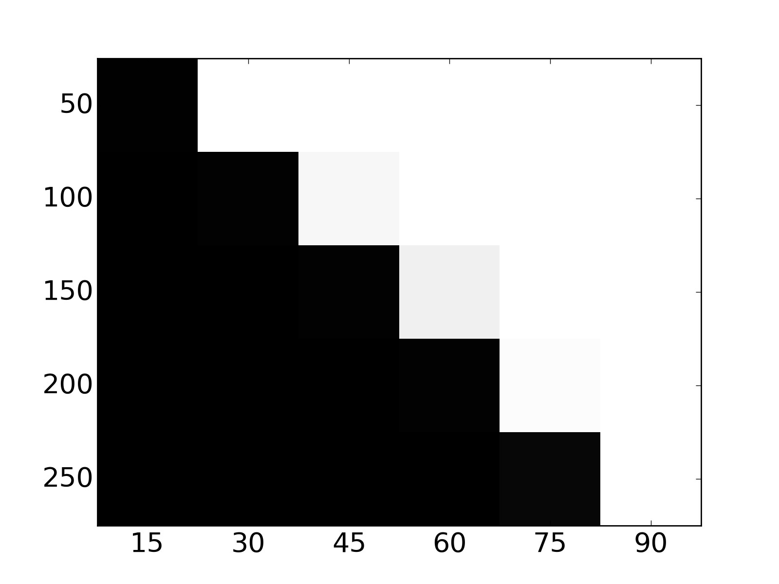
Figure 2: Success probabilities for the algorithms. yy axis is nn and xx axis is τ\tau. Black means fail.
Refer to caption

α=1.1\alpha=1.1

Refer to caption

α=1.5\alpha=1.5

Refer to caption

α=2\alpha=2

Figure 3: Rate of Convergence. τ=α​n34\tau=\alpha n^{\frac{3}{4}}, xx axis is the number of iterations, yy axis is the expected correlation with signal 𝒗\bm{v} (with variance represented as error bars)

For brevity we refer to our Tensor PCA with homotopy initialization method (Algorithm 1) as HomotopyPCA. We compare that with two other algorithms: the Flatten algorithm and the Power method. The Flatten algorithm was originally proposed by [14], where they show it works when τ=Ω⁡(n)\tau=\Omega(n). [18] accelerated the Flatten algorithm to near-linear time, and improved the analysis to show it works when τ=Ω~​(n3/4)\tau=\tilde{\Omega}(n^{3/4}). The Power method is similar to our algorithm, except it does not use intuitions from homotopy, and initialize at a random vector. Note that there are other algorithms proposed in [18], however they are based on the Sum-of-Squares SDP hierarchy, and even the fastest version runs in time O⁡(n5)O(n^{5}) (much worse than the O⁡(n3)O(n^{3}) algorithms compared here).

We first compare how often these algorithms successfully find the signal vector vv, given different values of τ\tau and nn. The results are in Figure 2, in which yy-axis represents nn and xx-axis represents τ\tau. We run 50 experiments for each values of (n,τ)(n,\tau), and the grayness in each grid shows how frequent each algorithm succeeds: black stands for “always fail” and white stands “always succeed”. For every algorithm, we say it fails if (1) when it converges, i.e., the result at two consecutive iterations are very close, the correlation with the signal 𝒗\bm{v} is less than 80%80\%; (2) the number of iterations exceeds 100. In the experiments for Power Method, we observe there are many cases where situation (1) is true, although our new algorithms can always find the correct solution. In these cases the function indeed have a local maximizer. From Figure 2, our algorithm outperforms both Power Method and the Flatten algorithm in practice. This suggests the constant hiding in our algorithm is possibly smaller.

Next we compare the number of iterations to converge with n=500n=500 and τ=α​n34\tau=\alpha n^{\frac{3}{4}}, where α\alpha varies in [1.1,1.5,2][1.1,1.5,2]. In Figure 3, the x-axis is the number of iterations, and the yy axis is the correlation with the signal 𝒗\bm{v} (error bars shows the distribution from 50 independent runs). For all α\alpha, Homotopy PCA performs well — converges in less than 55 iterations and finds the signal 𝒗\bm{v}. The Power Method converges to a result with good correlations with the signal 𝒗\bm{v}, but has large variance because it sometimes gets trapped in local optima. As for the Flatten algorithm, the algorithm always converges. However, it takes more iterations compared to our algorithm. Also when α\alpha is small, the converged result has bad correlation with 𝒗\bm{v}.

References

  • [1] Rong Ge, Jason D Lee, and Tengyu Ma. Matrix completion has no spurious local minimum. arXiv preprint arXiv:1605.07272, 2016.
  • [2] Animashree Anandkumar, Rong Ge, Daniel Hsu, Sham M Kakade, and Matus Telgarsky. Tensor decompositions for learning latent variable models. Journal of Machine Learning Research, 15(1):2773–2832, 2014.
  • [3] Rong Ge, Furong Huang, Chi Jin, and Yang Yuan. Escaping from saddle points—online stochastic gradient for tensor decomposition. In Proceedings of The 28th Conference on Learning Theory, pages 797–842, 2015.
  • [4] Ju Sun, Qing Qu, and John Wright. A geometric analysis of phase retrieval. Arxiv, 1602.06664, 2016.
  • [5] Ju Sun, Qing Qu, and John Wright. Complete dictionary recovery over the sphere. In Sampling Theory and Applications (SampTA), 2015 International Conference on, pages 407–410. IEEE, 2015.
  • [6] Sanjeev Arora, Rong Ge, and Ankur Moitra. New algorithms for learning incoherent and overcomplete dictionaries. In COLT, pages 779–806, 2014.
  • [7] Alekh Agarwal, Animashree Anandkumar, Prateek Jain, Praneeth Netrapalli, and Rashish Tandon. Learning sparsely used overcomplete dictionaries. In Proceedings of The 27th Conference on Learning Theory, pages 123–137, 2014.
  • [8] Animashree Anandkumar, Rong Ge, and Majid Janzamin. Learning overcomplete latent variable models through tensor methods. In Proceedings of The 28th Conference on Learning Theory, pages 36–112, 2015.
  • [9] Praneeth Netrapalli, UN Niranjan, Sujay Sanghavi, Animashree Anandkumar, and Prateek Jain. Non-convex robust pca. In Advances in Neural Information Processing Systems, pages 1107–1115, 2014.
  • [10] Xinyang Yi, Constantine Caramanis, and Sujay Sanghavi. Solving a mixture of many random linear equations by tensor decomposition and alternating minimization. Arxiv, abs/1608.05749, 2016.
  • [11] Hossein Mobahi and John W Fisher III. On the link between gaussian homotopy continuation and convex envelopes. In International Workshop on Energy Minimization Methods in Computer Vision and Pattern Recognition, pages 43–56. Springer, 2015.
  • [12] Hossein Mobahi and John W Fisher III. A theoretical analysis of optimization by gaussian continuation. In AAAI, pages 1205–1211. Citeseer, 2015.
  • [13] Elad Hazan, Kfir Y Levy, and Shai Shalev-Shwartz. On graduated optimization for stochastic non-convex problems. In International Conference on Machine Learning (ICML), 2016.
  • [14] Emile Richard and Andrea Montanari. A statistical model for tensor pca. In Advances in Neural Information Processing Systems, pages 2897–2905, 2014.
  • [15] Amelia Perry, Alexander S Wein, Afonso S Bandeira, and Ankur Moitra. Optimality and sub-optimality of pca for spiked random matrices and synchronization. arXiv preprint arXiv:1609.05573, 2016.
  • [16] Alex Bloemendal and Bálint Virág. Limits of spiked random matrices i. Probability Theory and Related Fields, 156(3-4):795–825, 2013.
  • [17] Quentin Berthet, Philippe Rigollet, et al. Optimal detection of sparse principal components in high dimension. The Annals of Statistics, 41(4):1780–1815, 2013.
  • [18] Samuel B Hopkins, Jonathan Shi, and David Steurer. Tensor principal component analysis via sum-of-square proofs. In Proceedings of The 28th Conference on Learning Theory, COLT, pages 3–6, 2015.
  • [19] Christopher J Hillar and Lek-Heng Lim. Most tensor problems are np-hard. Journal of the ACM (JACM), 60(6):45, 2013.
  • [20] Hossein Mobahi. Closed form for some gaussian convolutions. arXiv:1602.05610, 2016.
  • [21] Prateek Jain, Praneeth Netrapalli, and Sujay Sanghavi. Low-rank matrix completion using alternating minimization. In Proceedings of the forty-fifth annual ACM symposium on Theory of computing, pages 665–674. ACM, 2013.
  • [22] David L Donoho, Arian Maleki, and Andrea Montanari. Message-passing algorithms for compressed sensing. Proceedings of the National Academy of Sciences, 106(45):18914–18919, 2009.
  • [23] Adel Javanmard and Andrea Montanari. State evolution for general approximate message passing algorithms, with applications to spatial coupling. Information and Inference, page iat004, 2013.
  • [24] Anna Choromanska, Mikael Henaff, Michael Mathieu, Gérard Ben Arous, and Yann LeCun. The loss surfaces of multilayer networks. In AISTATS, 2015.
  • [25] Beatrice Laurent and Pascal Massart. Adaptive estimation of a quadratic functional by model selection. Annals of Statistics, pages 1302–1338, 2000.
  • [26] Ryota Tomioka and Taiji Suzuki. Spectral norm of random tensors. arXiv preprint arXiv:1407.1870, 2014.
  • [27] Michel Ledoux. Deviation inequalities on largest eigenvalues. In Geometric aspects of functional analysis, pages 167–219. Springer, 2007.

Appendix A Omitted Proofs

A.1 Omitted Proof in Section 2

Lemma 5 (Lemma 1 restated).
g⁡(𝒙,t)=τ​⟨𝒗,𝒙⟩3+t2​⟨3​τ​𝒗+𝒖,𝒙⟩+𝑨⁡(𝒙,𝒙,𝒙),g(\bm{x},t)=\tau\langle\bm{v},\bm{x}\rangle^{3}+t^{2}\langle 3\tau\bm{v}+\bm{u},\bm{x}\rangle+\bm{A}(\bm{x},\bm{x},\bm{x}),

where the vector 𝐮\bm{u} is defined by 𝐮j=∑i=1n(𝐀i​i​j+𝐀i​j​i+𝐀j​i​i)\bm{u}_{j}=\sum_{i=1}^{n}(\bm{A}_{iij}+\bm{A}_{iji}+\bm{A}_{jii}). Moreover, let 𝐳\bm{z} be a vector where 𝐳j=∑i=1d(𝐓i​i​j+𝐓i​j​i+𝐓j​i​i)\bm{z}_{j}=\sum_{i=1}^{d}(\bm{T}_{iij}+\bm{T}_{iji}+\bm{T}_{jii}), then we have 𝐳=3​τ​𝐯+𝐮\bm{z}=3\tau\bm{v}+\bm{u}.

Proof.

We can write g⁡(x,t)g(x,t) as an expectation

g⁡(𝒙,t)=∫ℝnf⁡(𝒙+𝒚)​kt​(𝒚)​𝑑y\displaystyle g(\bm{x},t)=\int_{\mathbb{R}^{n}}f(\bm{x}+\bm{y})k_{t}(\bm{y})dy =𝔼y∼N⁡(𝟎,t2​𝐈n)​[f⁡(𝒙+𝒚)]=𝔼y∼N⁡(𝟎,𝐈n)​[f⁡(𝒙+t​𝒚)]\displaystyle=\mathbb{E}_{y\sim N(\bm{0},t^{2}\mathbf{I}_{n})}[f(\bm{x}+\bm{y})]=\mathbb{E}_{y\sim N(\bm{0},\mathbf{I}_{n})}[f(\bm{x}+t\bm{y})]

Since ff is just a degree 3 polynomial, we can expand it and use the lower moments of Gaussian distributions:

g⁡(𝒙,t)\displaystyle g(\bm{x},t) =𝔼⁡[f⁡(𝒙+t​𝒚)]\displaystyle~=\mathbb{E}[f(\bm{x}+t\bm{y})]
=𝔼⁡[τ​⟨𝒗,(𝒙+𝒕​y)⟩3+𝑨⁡(𝒙+t​𝒚,𝒙+t​𝒚,𝒙+t​𝒚)]\displaystyle~=\mathbb{E}[\tau\langle\bm{v},(\bm{x}+\bm{t}y)\rangle^{3}+\bm{A}(\bm{x}+t\bm{y},\bm{x}+t\bm{y},\bm{x}+t\bm{y})]
=τ​⟨𝒗,𝒙⟩3+3​τ​t2​⟨𝒗,𝒙⟩⋅𝔼⁡[⟨𝒗,𝒚⟩2]+𝔼⁡[𝑨⁡(𝒙+t​𝒚,𝒙+t​𝒚,𝒙+t​𝒚)]\displaystyle~=\tau\langle\bm{v},\bm{x}\rangle^{3}+3\tau t^{2}\langle\bm{v},\bm{x}\rangle\cdot\mathbb{E}[\langle\bm{v},\bm{y}\rangle^{2}]+\mathbb{E}[\bm{A}(\bm{x}+t\bm{y},\bm{x}+t\bm{y},\bm{x}+t\bm{y})]
=τ​⟨𝒗,𝒙⟩3+3​τ​t2​⟨𝒗,𝒙⟩+t2​∑i,j(𝑨i​i​j+𝑨i​j​i+𝑨j​i​i)​𝒙j+𝑨⁡(𝒙,𝒙,𝒙)\displaystyle~=\tau\langle\bm{v},\bm{x}\rangle^{3}+3\tau t^{2}\langle\bm{v},\bm{x}\rangle+t^{2}\sum_{i,j}(\bm{A}_{iij}+\bm{A}_{iji}+\bm{A}_{jii})\bm{x}_{j}+\bm{A}(\bm{x},\bm{x},\bm{x})

Therefore the first part of the lemma holds if we define 𝒖\bm{u} to be the vector 𝒖j=∑i𝑨i​i​j+𝑨i​j​i+𝑨j​i​i\bm{u}_{j}=\sum_{i}\bm{A}_{iij}+\bm{A}_{iji}+\bm{A}_{jii}. In order to compute the vector 3​τ​𝒗+𝒖3\tau\bm{v}+\bm{u}, notice that the term ⟨3​τ​𝒗+𝒖,𝒙⟩\langle 3\tau\bm{v}+\bm{u},\bm{x}\rangle is the linear term on 𝒙\bm{x}, and it is equal to

⟨3​τ​𝒗+𝒖,𝒙⟩=𝔼y∼N⁡(𝟎,𝐈n)​[𝑻⁡(𝒙,𝒚,𝒚)+𝑻⁡(𝒚,𝒙,𝒚)+𝑻⁡(𝒚,𝒚,𝒙)].\langle 3\tau\bm{v}+\bm{u},\bm{x}\rangle=\mathbb{E}_{y\sim N(\bm{0},\mathbf{I}_{n})}[\bm{T}(\bm{x},\bm{y},\bm{y})+\bm{T}(\bm{y},\bm{x},\bm{y})+\bm{T}(\bm{y},\bm{y},\bm{x})].

This means

(3​τ​𝒗+𝒖)j=𝔼y∼N⁡(𝟎,𝐈n)​[𝑻⁡(𝒆j,𝒚,𝒚)+𝑻⁡(𝒚,𝒆j,𝒚)+𝑻⁡(𝒚,𝒚,𝒆j)]=∑i=1d(𝑻i​i​j+𝑻i​j​i+𝑻j​i​i).(3\tau\bm{v}+\bm{u})_{j}=\mathbb{E}_{y\sim N(\bm{0},\mathbf{I}_{n})}[\bm{T}(\bm{e}_{j},\bm{y},\bm{y})+\bm{T}(\bm{y},\bm{e}_{j},\bm{y})+\bm{T}(\bm{y},\bm{y},\bm{e}_{j})]=\sum_{i=1}^{d}(\bm{T}_{iij}+\bm{T}_{iji}+\bm{T}_{jii}).

∎

A.2 Omitted Proof in Section 3

Theorem A.1 (Theorem 3.1 restated).

When τ≥C​n3/4​log⁡n\tau\geq Cn^{3/4}\log n for a large enough constant CC, under the Independence Condition (Condition 3.1), Algorithm 1 finds a vector 𝐱m\bm{x}^{m} such that ⟨𝐱m,𝐯⟩≥0.8\langle\bm{x}^{m},\bm{v}\rangle\geq 0.8 in O⁡(log⁡log⁡n)O(\log\log n) iterations.

Algorithm 4 Tensor PCA by Homotopy Initialization
Input: Tensor 𝑻=τ⋅v⊗3+𝑨\bm{T}=\tau\cdot v^{\otimes 3}+\bm{A};
Output: Approximation of 𝒗\bm{v};
1 m=O⁡(log⁡log⁡n)m=O(\log\log n);
2 ∀j,𝒙j0=∑i𝑻i​i​j+𝑻i​j​i+𝑻j​i​i\forall~j,\bm{x}^{0}_{j}=\sum_{i}\bm{T}_{iij}+\bm{T}_{iji}+\bm{T}_{jii};
3 𝒙0=𝒙0/‖𝒙0‖\bm{x}^{0}=\bm{x}^{0}/\|\bm{x}^{0}\|; //𝒙0=𝒙†\bm{x}^{0}=\bm{x}^{\dagger}
4 for k=0k=0 to mm do
    5 𝒙k+1=𝑻(𝒙k,𝒙k,:)+𝑻(𝒙k,:,𝒙k)+𝑻(:,𝒙k,𝒙k)\bm{x}^{k+1}=\bm{T}(\bm{x}^{k},\bm{x}^{k},:)+\bm{T}(\bm{x}^{k},:,\bm{x}^{k})+\bm{T}(:,\bm{x}^{k},\bm{x}^{k});
    6 𝒙k+1=𝒙k+1/‖𝒙k+1‖\bm{x}^{k+1}=\bm{x}^{k+1}/\|\bm{x}^{k+1}\|;
7 return 𝒙m\bm{x}^{m};
Proof.

We first show the initial maximizer 𝒙0\bm{x}^{0} already has a nontrivial correlation with 𝒗\bm{v}. Recall 𝒙0=3​τ​𝒗+𝒖‖3​τ​𝒗+𝒖‖2\bm{x}^{0}=\frac{3\tau\bm{v}+\bm{u}}{\|3\tau\bm{v}+\bm{u}\|_{2}}. Note that if τ\tau is very large such that ‖3​τ​𝒗‖2≥10​‖u‖2\|3\tau\bm{v}\|_{2}\geq 10\|u\|_{2}, then we already have ⟨𝒙0,𝒗⟩≥0.8\langle\bm{x}^{0},\bm{v}\rangle\geq 0.8. Later we will show that whenever ⟨𝒙i,𝒗⟩≥0.8\langle\bm{x}^{i},\bm{v}\rangle\geq 0.8 all later iterations have the same property.

Therefore, we are left with the case when ‖𝒖‖2≥0.1​‖3​τ​𝒗‖2\|\bm{u}\|_{2}\geq 0.1\|3\tau\bm{v}\|_{2} (this implies τ≤O⁡(n)\tau\leq O(n)). In this case, by Condition 3.1 we know |⟨𝒖,𝒗⟩|=O⁡(n​m​log⁡n)|\langle\bm{u},\bm{v}\rangle|=O(\sqrt{nm\log n}) and ‖𝒖‖2=O⁡(n​m)\|\bm{u}\|_{2}=O(n\sqrt{m}), therefore

‖3​τ​𝒗+𝒖‖2∈[‖𝒖‖22+‖3​τ​𝒗‖22−O⁡(τ​n​m​log⁡n),‖𝒖‖22+‖3​τ​𝒗‖22+O⁡(τ​n​m​log⁡n)]\displaystyle\|3\tau\bm{v}+\bm{u}\|_{2}\in\left[\sqrt{\|\bm{u}\|_{2}^{2}+\|3\tau\bm{v}\|_{2}^{2}-O(\tau\sqrt{nm\log n})},\sqrt{\|\bm{u}\|_{2}^{2}+\|3\tau\bm{v}\|_{2}^{2}+O(\tau\sqrt{nm\log n})}\right]

Therefore, ‖3​τ​𝒗+𝒖‖2=Θ⁡(n​m)\|3\tau\bm{v}+\bm{u}\|_{2}=\Theta(n\sqrt{m}). Assume τ≥C​n3/4​logc​n\tau\geq Cn^{3/4}\log^{c}n for large enough CC (where we will later show c=1c=1 suffices)

⟨𝒙0,𝒗⟩=3​τ+⟨𝒖,𝒗⟩‖3​τ​𝒗+𝒖‖2=1O⁡(n​m)​Θ​(n34⋅logc⁡n)≥n−14⋅logc⁡nm.\displaystyle\langle\bm{x}^{0},\bm{v}\rangle=\frac{3\tau+\langle\bm{u},\bm{v}\rangle}{\|3\tau\bm{v}+\bm{u}\|_{2}}=\frac{1}{O(n\sqrt{m})}\Theta(n^{\frac{3}{4}}\cdot\log^{c}n)\geq\frac{n^{-\frac{1}{4}}\cdot\log^{c}n}{\sqrt{m}}.

Now let us consider the first step of power method. Let 𝒙^1\hat{\bm{x}}^{1} be the vector before normalization. Observe that 𝒙^1=3​τ​⟨𝒗,𝒙0⟩2​𝒗+δ⁡(𝒙0)\hat{\bm{x}}^{1}=3\tau\langle\bm{v},\bm{x}^{0}\rangle^{2}\bm{v}+\delta(\bm{x}^{0}). By Condition 3.1 we have bounds on ‖δ⁡(𝒙0)‖\|\delta(\bm{x}^{0})\| and |⟨δ⁡(𝒙0),v⟩||\langle\delta(\bm{x}^{0}),v\rangle|, therefore we have

⟨𝒙^1,𝒗⟩=3​τ​⟨𝒗,𝒙0⟩2+⟨δ⁡(𝒙0),𝒗⟩∈[3​τ​⟨𝒗,𝒙0⟩2−O⁡(m​log⁡n),3​τ​⟨𝒗,𝒙0⟩2+O⁡(m​log⁡n)].\displaystyle\langle\hat{\bm{x}}^{1},\bm{v}\rangle=3\tau\langle\bm{v},\bm{x}^{0}\rangle^{2}+\langle\delta(\bm{x}^{0}),\bm{v}\rangle\in\left[3\tau\langle\bm{v},\bm{x}^{0}\rangle^{2}-O(\sqrt{m\log n}),3\tau\langle\bm{v},\bm{x}^{0}\rangle^{2}+O(\sqrt{m\log n})\right].

Note that when τ≥C​n3/4​logc​n\tau\geq Cn^{3/4}\log^{c}n and logc⁡n≫m\log^{c}n\gg m, the first term is much larger than m​log⁡n\sqrt{m\log n}. Hence for the first iteration, we have ⟨𝒙^1,𝒗⟩≥(3−o⁡(1))​τ​⟨𝒗,𝒙0⟩2≥2​C​n14⋅log3​c⁡n/m\langle\hat{\bm{x}}^{1},\bm{v}\rangle\geq(3-o(1))\tau\langle\bm{v},\bm{x}^{0}\rangle^{2}\geq 2Cn^{\frac{1}{4}}\cdot\log^{3c}n/m.

Similar as before, when ‖δ⁡(𝒙0)‖2≤0.1​‖3​τ​⟨v,𝒙0⟩2​v‖2\|\delta(\bm{x}^{0})\|_{2}\leq 0.1\|3\tau\langle v,\bm{x}^{0}\rangle^{2}v\|_{2}, we already have ⟨𝒙1,𝒗⟩≥0.8\langle\bm{x}^{1},\bm{v}\rangle\geq 0.8. On the other hand, if ‖δ⁡(𝒙0)‖2≥0.1​‖3​τ​⟨v,𝒙0⟩2​v‖2\|\delta(\bm{x}^{0})\|_{2}\geq 0.1\|3\tau\langle v,\bm{x}^{0}\rangle^{2}v\|_{2}, in this case, by Condition 3.1 we know ‖δ⁡(𝒙^0)‖=O⁡(n​m)\|\delta(\hat{\bm{x}}^{0})\|=O(\sqrt{nm}). We again have ‖𝒙^1‖2∈‖δ⁡(𝒙0)‖22+‖3​τ​⟨𝒗,𝒙0⟩2​𝒗‖22±O⁡(τ​⟨𝒗,𝒙0⟩2​n​m)\|\hat{\bm{x}}^{1}\|_{2}\in\sqrt{\|\delta(\bm{x}^{0})\|_{2}^{2}+\|3\tau\langle\bm{v},\bm{x}^{0}\rangle^{2}\bm{v}\|_{2}^{2}\pm O(\tau\langle\bm{v},\bm{x}^{0}\rangle^{2}\sqrt{nm})}. Therefore, ‖𝒙^1‖2=O⁡(n​m)\|\hat{\bm{x}}^{1}\|_{2}=O(\sqrt{nm}). Combining the bounds for the norm of 𝒙^1\hat{\bm{x}}^{1} and its correlation with 𝒗\bm{v},

⟨𝒙^1‖𝒙^1‖,𝒗⟩≥n−14⋅log3​c⁡n/m32.\langle\frac{\hat{\bm{x}}^{1}}{\|\hat{\bm{x}}^{1}\|},\bm{v}\rangle\geq n^{-\frac{1}{4}}\cdot\log^{3c}n/m^{\frac{3}{2}}.

Therefore, when logc⁡n≫m\log^{c}n\gg m, the correlation between 𝒙1\bm{x}^{1} and 𝒗\bm{v} is larger than the correlation between 𝒙0\bm{x}^{0} and 𝒗\bm{v}. This shows the first step makes an improvement.

In order to show this for the future steps, we do induction over pp. The induction hypothesis is for every pp, either ⟨𝒙p,𝒗⟩≥0.8\langle\bm{x}^{p},\bm{v}\rangle\geq 0.8 or

⟨𝒙p,𝒗⟩≥n−14​log3p​c​n/m2p−12.\langle\bm{x}^{p},\bm{v}\rangle\geq n^{-\frac{1}{4}}\log^{3^{p}c}n/m^{2^{p}-\frac{1}{2}}.

Initially, for p=0p=0, we have already proved the induction hypothesis.

Now assume the induction hypothesis is true for pp. In the next iteration, let 𝒙^p+1\hat{\bm{x}}^{p+1} be the vector before normalization. Similar as before we have 𝒙^p+1=3​τ​⟨𝒗,𝒙p⟩2​𝒗+δ⁡(𝒙p)\hat{\bm{x}}^{p+1}=3\tau\langle\bm{v},\bm{x}^{p}\rangle^{2}\bm{v}+\delta(\bm{x}^{p}).

When ⟨𝒙p,𝒗⟩≥0.8\langle\bm{x}^{p},\bm{v}\rangle\geq 0.8, by Condition 3.1 we know the norm of ‖δ⁡(𝒙p)‖\|\delta(\bm{x}^{p})\| is much smaller than 3​τ​⟨𝒙p,𝒗⟩23\tau\langle\bm{x}^{p},\bm{v}\rangle^{2}. Therefore we still have ⟨𝒙p+1,𝒗⟩≥0.8\langle\bm{x}^{p+1},\bm{v}\rangle\geq 0.8.

In the other case, we follow the same strategy as the first step. By Condition 3.1 we can compute the correlation between 𝒙^p+1\hat{\bm{x}}^{p+1} and 𝒗\bm{v}:

⟨𝒙^p+1,𝒗⟩\displaystyle\langle\hat{\bm{x}}^{p+1},\bm{v}\rangle =3​τ​⟨𝒗,𝒙p⟩2±O⁡(m​log⁡n)\displaystyle=3\tau\langle\bm{v},\bm{x}^{p}\rangle^{2}\pm O(\sqrt{m\log n})
≥2​C​n14​log3p+1​c​n/m2p+1−1.\displaystyle\geq 2Cn^{\frac{1}{4}}\log^{3^{p+1}c}n/m^{2^{p+1}-1}.

For the norm of 𝒙^p+1\hat{\bm{x}}^{p+1}, notice that the first term 3​τ​⟨𝒗,𝒙p⟩2​𝒗3\tau\langle\bm{v},\bm{x}^{p}\rangle^{2}\bm{v} has norm 3​τ​⟨𝒗,𝒙p⟩23\tau\langle\bm{v},\bm{x}^{p}\rangle^{2}, and the second term δ⁡(𝒙p)\delta(\bm{x}^{p}) has norm Θ⁡(n​m)\Theta(\sqrt{nm}). Note that these two terms are almost orthogonal by Independence Condition, therefore

‖𝒙^p+1‖2=Θ⁡(τ​⟨𝒗,𝒙p⟩2)+O⁡(n​m)\|\hat{\bm{x}}^{p+1}\|_{2}=\Theta(\tau\langle\bm{v},\bm{x}^{p}\rangle^{2})+O(\sqrt{nm})

If 3​τ​⟨𝒗,𝒙p⟩2≥Δ​n​m3\tau\langle\bm{v},\bm{x}^{p}\rangle^{2}\geq\Delta\sqrt{nm}, then ‖𝒙^p+1‖2≤(3+Δ′)​τ​⟨𝒗,𝒙p⟩2\|\hat{\bm{x}}^{p+1}\|_{2}\leq(3+\Delta^{\prime})\tau\langle\bm{v},\bm{x}^{p}\rangle^{2}, where Δ′\Delta^{\prime} is a constant that is smaller than 0.10.1 when Δ\Delta is large enough. Therefore in this case ⟨𝒙^p+1‖𝒙^p+1‖2,𝒗⟩≥0.8\langle\frac{\hat{\bm{x}}^{p+1}}{\|\hat{\bm{x}}^{p+1}\|_{2}},\bm{v}\rangle\geq 0.8. Thus we successfully recover 𝒗\bm{v} in the next step.

Otherwise, we know ‖𝒙^p+1‖2=O⁡(n​m)\|\hat{\bm{x}}^{p+1}\|_{2}=O(\sqrt{nm}). Then,

⟨𝒙^p+1‖𝒙^p+1‖2,𝒗⟩≥n−14⋅log3p+1​c⁡n/m2p+1−12\langle\frac{\hat{\bm{x}}^{p+1}}{\|\hat{\bm{x}}^{p+1}\|_{2}},\bm{v}\rangle\geq n^{-\frac{1}{4}}\cdot\log^{3^{p+1}c}n/m^{2^{p+1}-\frac{1}{2}}

If we select c=1c=1, after m=O⁡(log⁡log⁡n)m=O(\log\log n) rounds, we have ⟨𝒙p,𝒗⟩≥n−14​log3p​c​n/m2p−12≥0.8\langle\bm{x}^{p},\bm{v}\rangle\geq n^{-\frac{1}{4}}\log^{3^{p}c}n/m^{2^{p}-\frac{1}{2}}\geq 0.8, therefore we must always be in the first case. As a result ⟨𝒙m,𝒗⟩≥0.8\langle\bm{x}^{m},\bm{v}\rangle\geq 0.8. ∎

Lemma 6 (Lemma 2 restated).

Let the sequence 𝐓0,⋯,𝐓m−1\bm{T}^{0},\cdots,\bm{T}^{m-1} be generated according to Section 3.1. Let 𝐐i=τ​𝐯⊗3+𝐂i\bm{Q}^{i}=\tau\bm{v}^{\otimes 3}+\bm{C}^{i}, where 𝐂i\bm{C}^{i}’s are tensors with independent Gaussian entries. Each entry in 𝐂i\bm{C}^{i} is distributed as N⁡(0,m)N(0,m). The two sets of variables {𝐓i}\{\bm{T}^{i}\} and {𝐐i}\{\bm{Q}^{i}\} has the same distribution.

Proof.

Note that both distributions are multivariate Gaussians. Therefore we only need to show that they have the same first and second moments.

For the first moment, this is easy, we have 𝔼⁡[𝑻p]=τ⋅v⊗3\mathbb{E}[\bm{T}^{p}]=\tau\cdot v^{\otimes 3} and 𝔼⁡[𝑸p]=τ⋅v⊗3\mathbb{E}[\bm{Q}^{p}]=\tau\cdot v^{\otimes 3} for all pp.

For the second moment (covariance), we consider the covariance between Ti​j​kpT^{p}_{ijk} and Ti′​j′​k′qT^{q}_{i^{\prime}j^{\prime}k^{\prime}}. Note that for the distribution QQ, as long as the 4 tuple (p,i,j,k)≠(q,i′,j′,k′)(p,i,j,k)\neq(q,i^{\prime},j^{\prime},k^{\prime}) the correlation is 0. We first show when (i,j,k)≠(i′,j′,k′)(i,j,k)\neq(i^{\prime},j^{\prime},k^{\prime}) we have

Cov⁡(𝑻i​j​kp,𝑻i′​j′​k′q)=\displaystyle\mathrm{Cov}(\bm{T}^{p}_{ijk},\bm{T}^{q}_{i^{\prime}j^{\prime}k^{\prime}})= 𝔼⁡[(𝑻i​j​kp−τ​𝒗i​𝒗j​𝒗k)​(𝑻i′​j′​k′q−τ​𝒗i′​𝒗j′​𝒗k′)]\displaystyle~\mathbb{E}[(\bm{T}^{p}_{ijk}-\tau\bm{v}_{i}\bm{v}_{j}\bm{v}_{k})(\bm{T}^{q}_{i^{\prime}j^{\prime}k^{\prime}}-\tau\bm{v}_{i^{\prime}}\bm{v}_{j^{\prime}}\bm{v}_{k^{\prime}})]
=\displaystyle= 𝔼⁡[(𝑩i​j​kp−𝑩i​j​k¯+𝑨i​j​k)​(𝑩i′​j′​k′q−𝑩i′​j′​k′¯+𝑨i′​j′​k′)]\displaystyle~\mathbb{E}[(\bm{B}^{p}_{ijk}-\overline{\bm{B}_{ijk}}+\bm{A}_{ijk})(\bm{B}^{q}_{i^{\prime}j^{\prime}k^{\prime}}-\overline{\bm{B}_{i^{\prime}j^{\prime}k^{\prime}}}+\bm{A}_{i^{\prime}j^{\prime}k^{\prime}})]
=\displaystyle= 𝔼⁡[𝑩i​j​kp−𝑩i​j​k¯+𝑨i​j​k]​𝔼​[𝑩i′​j′​k′q−𝑩i′​j′​k′¯+𝑨i′​j′​k′]\displaystyle~\mathbb{E}[\bm{B}^{p}_{ijk}-\overline{\bm{B}_{ijk}}+\bm{A}_{ijk}]\mathbb{E}[\bm{B}^{q}_{i^{\prime}j^{\prime}k^{\prime}}-\overline{\bm{B}_{i^{\prime}j^{\prime}k^{\prime}}}+\bm{A}_{i^{\prime}j^{\prime}k^{\prime}}]
=\displaystyle= 0\displaystyle~0

Hence for these variables the two distributions have the same covariance.

Next we consider the case p≠qp\neq q,

Cov⁡(𝑻i​j​kp,𝑻i​j​kq)=\displaystyle\mathrm{Cov}(\bm{T}^{p}_{ijk},\bm{T}^{q}_{ijk})= 𝔼⁡[(𝑻i​j​kp−τ​𝒗i​𝒗j​𝒗k)​(𝑻i​j​kq−τ​𝒗i​𝒗j​𝒗k)]\displaystyle~\mathbb{E}[(\bm{T}^{p}_{ijk}-\tau\bm{v}_{i}\bm{v}_{j}\bm{v}_{k})(\bm{T}^{q}_{ijk}-\tau\bm{v}_{i}\bm{v}_{j}\bm{v}_{k})]
=\displaystyle= 𝔼⁡[(𝑩i​j​kp−𝑩i​j​k¯+𝑨i​j​k)​(𝑩i​j​kq−𝑩i​j​k¯+𝑨i​j​k)]\displaystyle~\mathbb{E}[(\bm{B}^{p}_{ijk}-\overline{\bm{B}_{ijk}}+\bm{A}_{ijk})(\bm{B}^{q}_{ijk}-\overline{\bm{B}_{ijk}}+\bm{A}_{ijk})]
=\displaystyle= −m−1m2​𝔼​[(𝑩i​j​kp)2+(𝑩i​j​kq)2]+∑l≠p,q1m2​𝔼​[(𝑩i​j​kl)2]+𝔼⁡[𝑨i​j​k2]\displaystyle~-\frac{m-1}{m^{2}}\mathbb{E}[(\bm{B}^{p}_{ijk})^{2}+(\bm{B}^{q}_{ijk})^{2}]+\sum_{l\neq p,q}\frac{1}{m^{2}}\mathbb{E}[(\bm{B}^{l}_{ijk})^{2}]+\mathbb{E}[\bm{A}_{ijk}^{2}]
=\displaystyle= −2​(m−1)m2⋅m+m−2m2⋅m+1=0\displaystyle~-\frac{2(m-1)}{m^{2}}\cdot m+\frac{m-2}{m^{2}}\cdot m+1=0

The covariance for these entries also match.

Finally we need to consider the variance for each entry of 𝑻p\bm{T}^{p} and 𝑸p\bm{Q}^{p}. To do that we compute the Variance of 𝑻i​j​kp\bm{T}^{p}_{ijk}

Var⁡(𝑻i​j​kp)=\displaystyle\mathrm{Var}(\bm{T}^{p}_{ijk})= 𝔼⁡[(𝑻i​j​kp−τ​𝒗i​𝒗j​𝒗k)​(𝑻i​j​kp−τ​𝒗i​𝒗j​𝒗k)]\displaystyle~\mathbb{E}[(\bm{T}^{p}_{ijk}-\tau\bm{v}_{i}\bm{v}_{j}\bm{v}_{k})(\bm{T}^{p}_{ijk}-\tau\bm{v}_{i}\bm{v}_{j}\bm{v}_{k})]
=\displaystyle= 𝔼⁡[(𝑩i​j​kp−𝑩i​j​k¯+𝑨i​j​k)​(𝑩i​j​kp−𝑩i​j​k¯+𝑨i​j​k)]\displaystyle~\mathbb{E}[(\bm{B}^{p}_{ijk}-\overline{\bm{B}_{ijk}}+\bm{A}_{ijk})(\bm{B}^{p}_{ijk}-\overline{\bm{B}_{ijk}}+\bm{A}_{ijk})]
=\displaystyle= (m−1)2m2​𝔼​[(𝑩i​j​kp)2]+∑l≠p1m2​𝔼​[(𝑩i​j​kl)2]+𝔼⁡[𝑨i​j​k2]\displaystyle~\frac{(m-1)^{2}}{m^{2}}\mathbb{E}[(\bm{B}^{p}_{ijk})^{2}]+\sum_{l\neq p}\frac{1}{m^{2}}\mathbb{E}[(\bm{B}^{l}_{ijk})^{2}]+\mathbb{E}[\bm{A}_{ijk}^{2}]
=\displaystyle= (m−1)2m2⋅m+m−1m2⋅m+1=m\displaystyle~\frac{(m-1)^{2}}{m^{2}}\cdot m+\frac{m-1}{m^{2}}\cdot m+1=m

This is also the same as the variance of Qi​j​kpQ^{p}_{ijk}. Therefore the two multivariate Gaussians have the same mean and covariance, and must be the same distribution. ∎

Lemma 7 (Lemma 3 restated).

Let 𝐓p\bm{T}^{p} be generated according to Algorithm 2 and 𝐀p=𝐓p−τ​𝐯⊗3\bm{A}^{p}=\bm{T}^{p}-\tau\bm{v}^{\otimes 3}. Let 𝐮0\bm{u}^{0} be a vector such that 𝐮j0=∑i𝐀i​i​j0+𝐀i​j​i0+𝐀j​i​i0\bm{u}^{0}_{j}=\sum_{i}\bm{A}_{iij}^{0}+\bm{A}_{iji}^{0}+\bm{A}_{jii}^{0}, and δp(𝐱p)=𝐀p(𝐱p,𝐱p,:)+𝐀p(𝐱p,:,𝐱p)+𝐀p(:,𝐱p,𝐱p)\delta^{p}(\bm{x}^{p})=\bm{A}^{p}(\bm{x}^{p},\bm{x}^{p},:)+\bm{A}^{p}(\bm{x}^{p},:,\bm{x}^{p})+\bm{A}^{p}(:,\bm{x}^{p},\bm{x}^{p}). With high probability, (1) ‖𝐮0‖2=Θ⁡(n​m)\|\bm{u}^{0}\|_{2}=\Theta(n\sqrt{m}) and |⟨𝐮0,𝐯⟩|=O⁡(n​m​log⁡n)|\langle\bm{u}^{0},\bm{v}\rangle|=O(\sqrt{nm\log n}); (2) for the sequence computed by Algorithm 2, 𝐱0,𝐱1,⋯,𝐱m−1\bm{x}^{0},\bm{x}^{1},\cdots,\bm{x}^{m-1}, ∀0≤p≤m−1\forall~0\leq p\leq m-1, ‖δp​(𝐱p)‖2=Θ⁡(n​m)​‖𝐱p‖22\|\delta^{p}(\bm{x}^{p})\|_{2}=\Theta(\sqrt{nm})\|\bm{x}^{p}\|_{2}^{2} and |⟨δp​(𝐱p),𝐯⟩|=O⁡(m​log⁡n)​‖𝐱p‖22|\langle\delta^{p}(\bm{x}^{p}),\bm{v}\rangle|=O(\sqrt{m\log n})\|\bm{x}^{p}\|_{2}^{2}. As a result Condition 3.1 is satisfied.

Proof.

Since by Lemma 2, we know the noise tensors 𝑨p\bm{A}^{p} used in pp-th step behave exactly the same as independent Gaussian tensors. The vectors 𝒖0\bm{u}^{0} and δ⁡(xp)\delta(x^{p}) are therefore spherical Gaussian random variables conditioned on any value of 𝒙i\bm{x}^{i}. Therefore we can prove this lemma by standard Gaussian concentration results.

Claim 1.

[25] Suppose 𝐱\bm{x} is a dd-dimensional spherical Gaussian, then

Pr[|∥𝒙∥2−𝔼[∥𝒙∥2]|≥12𝔼[∥𝒙∥2]]≤e−Ω⁡(d).\Pr[|\|\bm{x}\|^{2}-\mathbb{E}[\|\bm{x}\|^{2}]|\geq\frac{1}{2}\mathbb{E}[\|\bm{x}\|^{2}]]\leq e^{-\Omega(d)}.

Also, for any fixed vector 𝐯\bm{v}, ⟨𝐱,𝐯⟩\langle\bm{x},\bm{v}\rangle is also a Gaussian distribution that satisfies

Pr[|⟨𝒙,𝒗⟩|≥t𝔼⁡[⟨𝒙,𝒗⟩2]]≤e−Ω⁡(t2).\Pr[|\langle\bm{x},\bm{v}\rangle|\geq t\sqrt{\mathbb{E}[\langle\bm{x},\bm{v}\rangle^{2}]}]\leq e^{-\Omega(t^{2})}.

For terms like ‖𝒖p‖\|\bm{u}^{p}\| and ‖δ⁡(𝒙p)‖\|\delta(\bm{x}^{p})\|, we know the norm of a Gaussian random variable obeys the χ2\chi^{2} distribution and is highly concentrated to its expectation. For terms like ⟨𝒖p,𝒗⟩\langle\bm{u}^{p},\bm{v}\rangle and ⟨δ⁡(𝒙p),𝒗⟩\langle\delta(\bm{x}^{p}),\bm{v}\rangle, we know they are just Gaussian distributions and is always bounded by O⁡(σ​log⁡n)O(\sigma\sqrt{\log n}) with high probability. Therefore we only need to compute the expected norms of these vectors.

𝔼⁡[‖𝒖p‖22]\displaystyle\mathbb{E}[\|\bm{u}^{p}\|_{2}^{2}] =𝔼⁡[∑j(∑i𝑨i​i​jp+𝑨i​j​ip+𝑨j​i​ip)2]\displaystyle~=\mathbb{E}[\sum_{j}(\sum_{i}\bm{A}^{p}_{iij}+\bm{A}^{p}_{iji}+\bm{A}^{p}_{jii})^{2}]
=𝔼⁡[∑j(∑i≠j(𝑨i​i​jp)2+(𝑨i​j​ip)2+(𝑨j​i​ip)2)+9​(𝑨j​j​jp)2]\displaystyle~=\mathbb{E}[\sum_{j}(\sum_{i\neq j}(\bm{A}^{p}_{iij})^{2}+(\bm{A}^{p}_{iji})^{2}+(\bm{A}^{p}_{jii})^{2})+9(\bm{A}^{p}_{jjj})^{2}]
=3​n​(n−1)​m+9​n​m\displaystyle~=3n(n-1)m+9nm
=Θ⁡(n2​m)\displaystyle~=\Theta(n^{2}m)

Therefore by Claim 1 we have ‖u‖2=Θ⁡(n​m)\|u\|_{2}=\Theta(n\sqrt{m}) with high probability.

𝔼⁡[⟨𝒖p,𝒗⟩]=𝔼⁡[∑j(∑i𝑨i​i​jp+𝑨i​j​ip+𝑨j​i​ip)​𝒗j]=0\displaystyle\mathbb{E}[\langle\bm{u}^{p},\bm{v}\rangle]=\mathbb{E}[\sum_{j}(\sum_{i}\bm{A}^{p}_{iij}+\bm{A}^{p}_{iji}+\bm{A}^{p}_{jii})\bm{v}_{j}]=0
𝔼⁡[⟨𝒖p,𝒗⟩2]\displaystyle\mathbb{E}[\langle\bm{u}^{p},\bm{v}\rangle^{2}] =𝔼⁡[∑j((∑i𝑨i​i​jp+𝑨i​j​ip+𝑨j​i​ip)​𝒗j)2]\displaystyle~=\mathbb{E}[\sum_{j}((\sum_{i}\bm{A}^{p}_{iij}+\bm{A}^{p}_{iji}+\bm{A}^{p}_{jii})\bm{v}_{j})^{2}]
=𝔼⁡[∑j𝒗j2​(9​(𝑨j​j​jp)2+∑i≠j(𝑨i​i​jp)2+(𝑨i​j​ip)2+(𝑨j​i​ip)2)]\displaystyle~=\mathbb{E}[\sum_{j}\bm{v}_{j}^{2}(9(\bm{A}^{p}_{jjj})^{2}+\sum_{i\neq j}(\bm{A}^{p}_{iij})^{2}+(\bm{A}^{p}_{iji})^{2}+(\bm{A}^{p}_{jii})^{2})]
=9​m+3​(n−1)​m\displaystyle~=9m+3(n-1)m
=Θ⁡(n​m)\displaystyle~=\Theta(nm)

This means ⟨u,v⟩\langle u,v\rangle is a Gaussian random variable with variance σ2=Θ⁡(n​m)\sigma^{2}=\Theta(nm), therefore for any constant C′C^{\prime}, with probability at least 1−n−C′1-n^{-C^{\prime}} we know |⟨u,v⟩|≤O⁡(n​m​log⁡n)|\langle u,v\rangle|\leq O(\sqrt{nm\log n}). We can apply union bound over all pp and get the desired result.

Similarly we can compute the expected square norm of δ⁡(𝒙p)\delta(\bm{x}^{p}) as below

𝔼⁡[‖δ⁡(𝒙p)‖22]\displaystyle\mathbb{E}[\|\delta(\bm{x}^{p})\|_{2}^{2}] =Θ(1)𝔼[∥𝑨p(𝒙p,𝒙p,:)∥22]\displaystyle~=\Theta(1)\mathbb{E}[\|\bm{A}^{p}(\bm{x}^{p},\bm{x}^{p},:)\|_{2}^{2}]
=Θ⁡(1)​𝔼​[∑k(∑i,j𝑨i​j​kp​𝒙ip​𝒙jp)2]\displaystyle~=\Theta(1)\mathbb{E}[\sum_{k}(\sum_{i,j}\bm{A}^{p}_{ijk}\bm{x}^{p}_{i}\bm{x}^{p}_{j})^{2}]
=Θ⁡(1)​𝔼​[∑k(∑i,j(𝑨i​j​kp)2​(𝒙ip)2​(𝒙jp)2)]\displaystyle~=\Theta(1)\mathbb{E}[\sum_{k}(\sum_{i,j}(\bm{A}^{p}_{ijk})^{2}(\bm{x}^{p}_{i})^{2}(\bm{x}^{p}_{j})^{2})]
=Θ⁡(1)​n​m​‖xp‖24\displaystyle~=\Theta(1)nm\|x^{p}\|_{2}^{4}
𝔼⁡[⟨δ⁡(𝒙p),𝒗⟩]=∑i,j,k𝔼⁡[𝑨i​j​kp​(𝒙ip​𝒙jp​𝒗k+𝒙ip​𝒗j​𝒙kp+𝒗i​𝒙jp​𝒙kp)]=0\displaystyle\mathbb{E}[\langle\delta(\bm{x}^{p}),\bm{v}\rangle]=\sum_{i,j,k}\mathbb{E}[\bm{A}^{p}_{ijk}(\bm{x}^{p}_{i}\bm{x}^{p}_{j}\bm{v}_{k}+\bm{x}^{p}_{i}\bm{v}_{j}\bm{x}^{p}_{k}+\bm{v}_{i}\bm{x}^{p}_{j}\bm{x}^{p}_{k})]=0
𝔼⁡[⟨δ⁡(𝒙p),𝒗⟩2]\displaystyle\mathbb{E}[\langle\delta(\bm{x}^{p}),\bm{v}\rangle^{2}] =∑i,j,k𝔼⁡[(𝑨i​j​kp)2​(𝒙ip​𝒙jp​𝒗k+𝒙ip​𝒗j​𝒙kp+𝒗i​𝒙jp​𝒙kp)2]\displaystyle~=\sum_{i,j,k}\mathbb{E}[(\bm{A}^{p}_{ijk})^{2}(\bm{x}^{p}_{i}\bm{x}^{p}_{j}\bm{v}_{k}+\bm{x}^{p}_{i}\bm{v}_{j}\bm{x}^{p}_{k}+\bm{v}_{i}\bm{x}^{p}_{j}\bm{x}^{p}_{k})^{2}]
=3​m​∑k𝒗k2​∑i,j(𝒙ip)2​(𝒙jp)2+6​m​∑i(𝒙ip)2​∑j,k𝒗i​𝒗j​𝒙jp​𝒙kp\displaystyle~=3m\sum_{k}\bm{v}_{k}^{2}\sum_{i,j}(\bm{x}_{i}^{p})^{2}(\bm{x}_{j}^{p})^{2}+6m\sum_{i}(\bm{x}_{i}^{p})^{2}\sum_{j,k}\bm{v}_{i}\bm{v}_{j}\bm{x}_{j}^{p}\bm{x}_{k}^{p}
=3​m​‖𝒙p‖24+6​‖𝒙p‖22​⟨𝒗,𝒙p⟩2\displaystyle~=3m\|\bm{x}^{p}\|_{2}^{4}+6\|\bm{x}^{p}\|_{2}^{2}\langle\bm{v},\bm{x}^{p}\rangle^{2}
≤9​m​‖𝒙p‖24\displaystyle~\leq 9m\|\bm{x}^{p}\|_{2}^{4}

The bounds on ‖δ⁡(𝒙p)‖\|\delta(\bm{x}^{p})\| and ⟨δ⁡(𝒙p),v⟩\langle\delta(\bm{x}^{p}),v\rangle follows immediately from these expectations. ∎

A.3 Omitted Proof in Section 4

Lemma 8 (Lemma 4 restated).

The smoothed version of the alternative objective is

gr​(𝒙,t)=τ​⟨𝒗,𝒙⟩3+t2​⟨3​τ​𝒗+𝒖,𝒙⟩+𝑨⁡(𝒙,𝒙,𝒙)−3​τ4​(‖x‖24+2​t2​(n+2)​‖x‖22+t4​(n2+2​n))\displaystyle g_{r}(\bm{x},t)=\tau\langle\bm{v},\bm{x}\rangle^{3}+t^{2}\langle 3\tau\bm{v}+\bm{u},\bm{x}\rangle+\bm{A}(\bm{x},\bm{x},\bm{x})-\frac{3\tau}{4}\left(\|x\|_{2}^{4}+2t^{2}(n+2)\|x\|_{2}^{2}+t^{4}(n^{2}+2n)\right)

Its gradient and Hessian are equal to

∇gr​(𝒙,t)=3​τ​⟨𝒗,𝒙⟩2​𝒗+t2​(3​τ​𝒗+𝒖)+δ⁡(𝒙)−3​τ​(‖𝒙‖22​𝒙+t2​(n+2)​𝒙).\displaystyle\nabla g_{r}(\bm{x},t)=3\tau\langle\bm{v},\bm{x}\rangle^{2}\bm{v}+t^{2}(3\tau\bm{v}+\bm{u})+\delta(\bm{x})-3\tau(\|\bm{x}\|_{2}^{2}\bm{x}+t^{2}(n+2)\bm{x}).

and

∇2gr(𝒙,t)=−3τ((∥𝒙∥22+t2(n+2))𝑰−2⟨𝒗,𝒙⟩𝒗𝒗T+2𝒙𝒙T)+Ps​y​m[𝑨(𝒙,:,:)+𝑨(:,𝒙,:)+𝑨(:,:,𝒙)].\displaystyle\nabla^{2}g_{r}(\bm{x},t)=-3\tau((\|\bm{x}\|_{2}^{2}+t^{2}(n+2))\bm{I}-2\langle\bm{v},\bm{x}\rangle\bm{v}\bm{v}^{T}+2\bm{x}\bm{x}^{T})+P_{sym}[\bm{A}(\bm{x},:,:)+\bm{A}(:,\bm{x},:)+\bm{A}(:,:,\bm{x})].
Proof.

Similar to Lemma 1, we can write the smoothing operation as an expectation. By linearity of expectation we know

gr​(𝒙,t)=g⁡(𝒙,t)+𝔼⁡[‖𝒙+t​𝒚‖24]g_{r}(\bm{x},t)=g(\bm{x},t)+\mathbb{E}[\|\bm{x}+t\bm{y}\|_{2}^{4}]

We can compute the new terms by the moments of Gaussians:

𝔼⁡[‖𝒙+t​𝒚‖24]\displaystyle\mathbb{E}[\|\bm{x}+t\bm{y}\|_{2}^{4}] =𝔼⁡[(‖𝒙‖22+2​t​⟨𝒙,𝒚⟩+t2​‖𝒚‖22)2]\displaystyle=\mathbb{E}[(\|\bm{x}\|_{2}^{2}+2t\langle\bm{x},\bm{y}\rangle+t^{2}\|\bm{y}\|_{2}^{2})^{2}]
=𝔼⁡[‖𝒙‖24+4​t2​⟨𝒙,𝒚⟩2+t4​‖𝒚‖24+2​t2​‖x‖2​‖y‖2]\displaystyle=\mathbb{E}[\|\bm{x}\|_{2}^{4}+4t^{2}\langle\bm{x},\bm{y}\rangle^{2}+t^{4}\|\bm{y}\|_{2}^{4}+2t^{2}\|x\|^{2}\|y\|^{2}]
=‖x‖24+t2​(2​n+4)​‖x‖22+t4​(n2+2​n)=‖x‖24+2​t2​(n+2)​‖x‖22+t4​(n2+2​n).\displaystyle=\|x\|_{2}^{4}+t^{2}(2n+4)\|x\|_{2}^{2}+t^{4}(n^{2}+2n)=\|x\|_{2}^{4}+2t^{2}(n+2)\|x\|_{2}^{2}+t^{4}(n^{2}+2n).

Here in the second equation we omitted all the odd order terms for 𝒚\bm{y} because those terms have expectation 0. The final step uses the moments of Gaussians.

The equation for gr​(𝒙,t)g_{r}(\bm{x},t) follows immediately, and since it is a polynomial it is easy to compute its gradient and Hessian. ∎

Before trying to characterize the local maxima on the homotopy path, let us first prove the following property for the matrix Ps​y​m[𝑨(𝒙,:,:)+𝑨(:,𝒙,:)+𝑨(:,:,𝒙)]P_{sym}[\bm{A}(\bm{x},:,:)+\bm{A}(:,\bm{x},:)+\bm{A}(:,:,\bm{x})].

Lemma 9.

Let H(𝐱)=Ps​y​m[𝐀(𝐱,:,:)+𝐀(:,𝐱,:)+𝐀(:,:,𝐱)]H(\bm{x})=P_{sym}[\bm{A}(\bm{x},:,:)+\bm{A}(:,\bm{x},:)+\bm{A}(:,:,\bm{x})], there exists constants c−,c+c^{-},c^{+} such that with probability at least 1−exp⁡(−Ω⁡(n))1-\exp(-\Omega(n)), for any unit vector 𝐱\bm{x} we have

c−​n≤λm​a​x≤c+​n.c^{-}\sqrt{n}\leq\lambda_{max}\leq c^{+}\sqrt{n}.
Proof.

For the upperbound, we use the bound on tensor spectral norm. [26] proved that for a random Gaussian tensor 𝑨\bm{A}, with probability at least 1−exp⁡(−Ω⁡(n))1-\exp(-\Omega(n)) we know for any vectors 𝒙,𝒚,𝒛\bm{x},\bm{y},\bm{z}, |𝑨⁡(𝒙,𝒚,𝒛)|≤O⁡(n)|\bm{A}(\bm{x},\bm{y},\bm{z})|\leq O(\sqrt{n}). Therefore for any unit vector 𝒚\bm{y}, |𝒚⊤​H​(𝒙)​𝒚|=|𝑨⁡(𝒙,𝒚,𝒚)+𝑨⁡(𝒚,𝒙,𝒚)+𝑨⁡(𝒚,𝒚,𝒙)|≤O⁡(n)|\bm{y}^{\top}H(\bm{x})\bm{y}|=|\bm{A}(\bm{x},\bm{y},\bm{y})+\bm{A}(\bm{y},\bm{x},\bm{y})+\bm{A}(\bm{y},\bm{y},\bm{x})|\leq O(\sqrt{n}).

For the lowerbound, we use the distribution of the largest eigenvalue of Gaussian Orthogonal Ensemble. Suppose 𝑴\bm{M} is a random matrix whose entries are i.i.d. standard Gaussians, then the symmetric matrix 𝑴+𝑴⊤2\frac{\bm{M}+\bm{M}^{\top}}{\sqrt{2}} is distributed according to the Gaussian Orthogonal Ensemble. Let P𝒙⟂P_{\bm{x}^{\perp}} be the projection operator to the orthogonal subspace of 𝒙\bm{x}, then the key observation is P𝒙⟂​H​(𝒙)​P𝒙⟂P_{\bm{x}^{\perp}}H(\bm{x})P_{\bm{x}^{\perp}} is (up to a constant scaling) distributed as a Gaussian Orthogonal Ensemble of dimension (n−1)×(n−1)(n-1)\times(n-1). To see this, the easiest way is to observe that Gaussians are invariant under rotation, so we can take 𝒙=𝒆1\bm{x}=\bm{e}_{1}. Now for i,j={2,3,…,n}i,j=\{2,3,...,n\}, [P𝒙⟂​H​(𝒙)​P𝒙⟂]i,j=𝑨1​i​j+𝑨1​j​i+𝑨i​1​j+𝑨j​1​i+𝑨i​j​1+𝑨j​i​1[P_{\bm{x}^{\perp}}H(\bm{x})P_{\bm{x}^{\perp}}]_{i,j}=\bm{A}_{1ij}+\bm{A}_{1ji}+\bm{A}_{i1j}+\bm{A}_{j1i}+\bm{A}_{ij1}+\bm{A}_{ji1}. The random entries 1​i​j,i​1​j,i​j​11ij,i1j,ij1 do not overlap because i,j≠1i,j\neq 1. Therefore the matrix is the sum of three Gaussian Orthogonal Ensembles, and by property of Gaussians that is equivalent to 3\sqrt{3} times a Gaussian Orthogonal Ensemble. Now, using the result in [27], we know for any fixed 𝒙\bm{x}, Pr[λm​a​x(P𝒙⟂H(𝒙)P𝒙⟂)≤n/2]≤1−exp(−Ω(n2))\Pr[\lambda_{max}(P_{\bm{x}^{\perp}}H(\bm{x})P_{\bm{x}^{\perp}})\leq\sqrt{n}/2]\leq 1-\exp(-\Omega(n^{2})). By standard covering argument (the ϵ\epsilon-net for nn dimensional vectors have size (n/ϵ)O⁡(n)(n/\epsilon)^{O(n)} which is much smaller than exp⁡(−Ω⁡(n2))\exp(-\Omega(n^{2}))), we know with high probability for all 𝒙\bm{x} λm​a​x​(P𝒙⟂​H​(𝒙)​P𝒙⟂)≥n/2\lambda_{max}(P_{\bm{x}^{\perp}}H(\bm{x})P_{\bm{x}^{\perp}})\geq\sqrt{n}/2. The lemma follows immediately because λm​a​x​(H⁡(𝒙))≥λm​a​x​(P𝒙⟂​H​(𝒙)​P𝒙⟂)\lambda_{max}(H(\bm{x}))\geq\lambda_{max}(P_{\bm{x}^{\perp}}H(\bm{x})P_{\bm{x}^{\perp}}). ∎

Now we are ready to prove Theorem 4.1. To capture the properties of the homotopy path, we break it into three lemmas.

Lemma 10.

When τ=n3/4​log⁡n\tau=n^{3/4}\log n, t≥C​n−1t\geq Cn^{-1} for large enough constant CC, there exists a local maximizer 𝐱t\bm{x}^{t} of gr​(𝐱,t)g_{r}(\bm{x},t) such that ‖𝐱t−𝐱†‖2=o⁡(1)​‖𝐱†‖2\|\bm{x}^{t}-\bm{x}^{\dagger}\|_{2}=o(1)\|\bm{x}^{\dagger}\|_{2}.

Proof.

Recall according to the objective we chose, the maximizer at infinity 𝒙†\bm{x}^{\dagger} can be computed explicitly and we know 𝒙†=3​τ​𝒗+𝒖3​τ​(n+2)\bm{x}^{\dagger}=\frac{3\tau\bm{v}+\bm{u}}{3\tau(n+2)}. By Conjecture 1, we can estimate the norm and correlation with 𝒗\bm{v}:

∥𝒙†∥2=Θ(n−3/4log−1n),⟨𝒙†,𝒗⟩=(1±o(1))/n.\|\bm{x}^{\dagger}\|_{2}=\Theta(n^{-3/4}\log^{-1}n),\quad\langle\bm{x}^{\dagger},\bm{v}\rangle=(1\pm o(1))/n.

We shall first prove in the region ℬ={𝒙:∥𝒙−𝒙†∥2≤12∥𝒙†∥2,⟨𝒙,𝒗⟩≤10/n}\mathcal{B}=\{\bm{x}:\|\bm{x}-\bm{x}^{\dagger}\|_{2}\leq\frac{1}{2}\|\bm{x}^{\dagger}\|_{2},\langle\bm{x},\bm{v}\rangle\leq 10/n\}, the Hessian of the objective function is always negative definite. By standard analysis in convex optimization, this in particular implies two things: 1. There can be at most one local maximizer in this region; 2. If the function is μ\mu-strongly-concave (∇2g​(𝒙,t)⪰−μ​I\nabla^{2}g(\bm{x},t)\succeq-\mu I), and a point 𝒙\bm{x} has ‖∇g​(𝒙,t)‖≤ϵ\|\nabla g(\bm{x},t)\|\leq\epsilon, then there is a local maximizer within ϵ/μ\epsilon/\mu. This particular implies if there is a point 𝒙\bm{x} in the interior ℬ′={𝒙:∥𝒙−𝒙†∥2≤14∥𝒙†∥2,⟨𝒙,𝒗⟩≤2/n}\mathcal{B}^{\prime}=\{\bm{x}:\|\bm{x}-\bm{x}^{\dagger}\|_{2}\leq\frac{1}{4}\|\bm{x}^{\dagger}\|_{2},\langle\bm{x},\bm{v}\rangle\leq 2/n\} such that ∇g​(𝒙,t)\nabla g(\bm{x},t) is very small, then there must exist a local maximizer in ℬ\mathcal{B}.

By Lemma 4, we know the Hessian is equal to:

∇2gr(𝒙,t)=−3τ((∥𝒙∥22+t2(n+2))𝑰−2⟨𝒗,𝒙⟩𝒗𝒗T+2𝒙𝒙T)+Ps​y​m[𝑨(𝒙,:,:)+𝑨(:,𝒙,:)+𝑨(:,:,𝒙)].\nabla^{2}g_{r}(\bm{x},t)=-3\tau((\|\bm{x}\|_{2}^{2}+t^{2}(n+2))\bm{I}-2\langle\bm{v},\bm{x}\rangle\bm{v}\bm{v}^{T}+2\bm{x}\bm{x}^{T})+P_{sym}[\bm{A}(\bm{x},:,:)+\bm{A}(:,\bm{x},:)+\bm{A}(:,:,\bm{x})].

In the region we are interested in, since ⟨𝒗,𝒙⟩≤10/n≤t2​(n+2)/2\langle\bm{v},\bm{x}\rangle\leq 10/n\leq t^{2}(n+2)/2 when CC is large enough, we have the first term

−3​τ​((‖𝒙‖22+t2​(n+2))​𝑰−2​⟨𝒗,𝒙⟩​𝒗​𝒗T+2​𝒙​𝒙T)⪯−1.5​τ​t2​(n+2)​𝑰.-3\tau((\|\bm{x}\|_{2}^{2}+t^{2}(n+2))\bm{I}-2\langle\bm{v},\bm{x}\rangle\bm{v}\bm{v}^{T}+2\bm{x}\bm{x}^{T})\preceq-1.5\tau t^{2}(n+2)\bm{I}.

On the other hand, for the second part we know by Lemma 9

Ps​y​m[𝑨(𝒙,:,:)+𝑨(:,𝒙,:)+𝑨(:,:,𝒙)]⪯12c+n∥𝒙†∥2I.P_{sym}[\bm{A}(\bm{x},:,:)+\bm{A}(:,\bm{x},:)+\bm{A}(:,:,\bm{x})]\preceq\frac{1}{2}c^{+}\sqrt{n}\|\bm{x}^{\dagger}\|_{2}I.

By our choice of parameters, τt2(n+2)=Ω(n−1/4logn)\tau t^{2}(n+2)=\Omega(n^{-1/4}\log n), and n∥𝒙†∥2=Θ(n−1/4log−1n)\sqrt{n}\|\bm{x}^{\dagger}\|_{2}=\Theta(n^{-1/4}\log^{-1}n), therefore the first term dominates and we know the Hessian ∇2gr​(𝒙,t)⪯−τ​t2​(n+2)​𝑰\nabla^{2}g_{r}(\bm{x},t)\preceq-\tau t^{2}(n+2)\bm{I}.

When tt is a large polynomial of nn (e.g. t=n10t=n^{10}), simple calculation shows the optima 𝒙t\bm{x}^{t} is very close to 𝒙†\bm{x}^{\dagger}, and we have 𝒙t∈ℬ′\bm{x}^{t}\in\mathcal{B^{\prime}}. When C/n≤t<n10C/n\leq t<n^{10}, let t0=n10t_{0}=n^{10}, select t1,t2,…,tqt_{1},t_{2},...,t_{q} such that tq=tt_{q}=t, and ti,ti+1t_{i},t_{i+1} are close enough that if 𝒙ti∈ℬ′\bm{x}^{t_{i}}\in\mathcal{B^{\prime}}, by strong concavity we can get 𝒙ti+1\bm{x}^{t_{i+1}} exists and 𝒙ti+1∈ℬ\bm{x}^{t_{i+1}}\in\mathcal{B}. We will prove 𝒙ti∈ℬ′\bm{x}^{t_{i}}\in\mathcal{B}^{\prime} by induction. The base case is already done.

Suppose 𝒙ti−1∈ℬ′\bm{x}^{t_{i-1}}\in\mathcal{B}^{\prime}, we know that 𝒙ti∈ℬ\bm{x}^{t_{i}}\in\mathcal{B}. We will use the first order condition to refine our knowledge about 𝒙ti\bm{x}^{t_{i}} and show 𝒙ti∈ℬ′\bm{x}^{t_{i}}\in\mathcal{B}^{\prime}. From (5), we can derive the expression of stationary points,

𝒙ti=3​τ​⟨𝒗,𝒙ti⟩2​𝒗+t2​(3​τ​𝒗+𝒖)+δ⁡(𝒙ti)3​τ​(‖𝒙ti‖22+t2​(n+2))\bm{x}^{t_{i}}=\frac{3\tau\langle\bm{v},\bm{x}^{t_{i}}\rangle^{2}\bm{v}+t^{2}(3\tau\bm{v}+\bm{u})+\delta(\bm{x}^{t_{i}})}{3\tau(\|\bm{x}^{t_{i}}\|_{2}^{2}+t^{2}(n+2))} (7)

Note that 𝒙ti\bm{x}^{t_{i}} is a stationary point on homotopy path, so it should satisfy Conjecture 1. We also know it is in ℬ\mathcal{B}.

Since t≥C​n−1t\geq Cn^{-1}, ‖τ​⟨𝒗,𝒙ti⟩2​𝒗‖2=Θ⁡(n−54​log⁡n)\|\tau\langle\bm{v},\bm{x}^{t_{i}}\rangle^{2}\bm{v}\|_{2}=\Theta(n^{-\frac{5}{4}}\log n), ‖t2​(3​τ​𝒗+𝒖)‖2≥Ω⁡(n−1)\|t^{2}(3\tau\bm{v}+\bm{u})\|_{2}\geq\Omega(n^{-1}) and ‖δ⁡(𝒙ti)‖2=Θ⁡(n−1​log−2​n)\|\delta(\bm{x}^{t_{i}})\|_{2}=\Theta(n^{-1}\log^{-2}n). Therefore, if we let 𝒘=3​τ​⟨𝒗,𝒙ti⟩2​𝒗+δ⁡(𝒙ti)\bm{w}=3\tau\langle\bm{v},\bm{x}^{t_{i}}\rangle^{2}\bm{v}+\delta(\bm{x}^{t_{i}}) we know ‖𝒘‖2≤o⁡(1)​‖t2​(3​τ​𝒗+𝒖)‖2\|\bm{w}\|_{2}\leq o(1)\|t^{2}(3\tau\bm{v}+\bm{u})\|_{2}. The middle term dominates the numerator. Moreover, t2​(n+2)≥Ω⁡(n−1)t^{2}(n+2)\geq\Omega(n^{-1}) and ∥𝒙ti∥22=Θ(n−3/2log−2n)\|\bm{x}^{t_{i}}\|_{2}^{2}=\Theta(n^{-3/2}\log^{-2}n), and thus, t2​nt^{2}n dominates the denominator. Now we have

𝒙ti\displaystyle\bm{x}^{t_{i}} =3​τ​⟨𝒗,𝒙ti⟩2​𝒗+t2​(3​τ​𝒗+𝒖)+δ⁡(𝒙ti)3​τ​(‖𝒙ti‖22+t2​(n+2))\displaystyle~=\frac{3\tau\langle\bm{v},\bm{x}^{t_{i}}\rangle^{2}\bm{v}+t^{2}(3\tau\bm{v}+\bm{u})+\delta(\bm{x}^{t_{i}})}{3\tau(\|\bm{x}^{t_{i}}\|_{2}^{2}+t^{2}(n+2))}
=t2​(3​τ​𝒗+𝒖)+𝒘3​τ​t2​(n+2)​(1+ϵ)\displaystyle~=\frac{t^{2}(3\tau\bm{v}+\bm{u})+\bm{w}}{3\tau t^{2}(n+2)(1+\epsilon)}
=3​τ​𝒗+𝒖3​τ​(n+2)⋅11+ϵ+𝒘3​τ​t2​(n+2)​(1+ϵ).\displaystyle~=\frac{3\tau\bm{v}+\bm{u}}{3\tau(n+2)}\cdot\frac{1}{1+\epsilon}+\frac{\bm{w}}{3\tau t^{2}(n+2)(1+\epsilon)}.
=𝒙†+𝒙†​(11+ϵ−1)+𝒘3​τ​t2​(n+2)​(1+ϵ).\displaystyle~=\bm{x}^{\dagger}+\bm{x}^{\dagger}(\frac{1}{1+\epsilon}-1)+\frac{\bm{w}}{3\tau t^{2}(n+2)(1+\epsilon)}.

Since ϵ=o⁡(1)\epsilon=o(1) and ‖w‖2≤o⁡(1)​‖t2​(3​τ​𝒗+𝒖)‖2\|w\|_{2}\leq o(1)\|t^{2}(3\tau\bm{v}+\bm{u})\|_{2}, we know the two additional term has norm o⁡(1)​‖𝒙†‖2o(1)\|\bm{x}^{\dagger}\|_{2}, therefore 𝒙ti\bm{x}^{t_{i}} is very close to 𝒙†\bm{x}^{\dagger}.

Next we bound the correlation with 𝒗\bm{v}. We know ⟨𝒗,𝒙ti⟩≤10/n\langle\bm{v},\bm{x}^{t_{i}}\rangle\leq 10/n because 𝒙ti∈ℬ\bm{x}^{t_{i}}\in\mathcal{B}. Also, the correlation between |⟨𝒖,𝒗⟩|=O⁡(n​log⁡n)|\langle\bm{u},\bm{v}\rangle|=O(\sqrt{n\log n}) and |⟨δ(𝒙ti),𝒗⟩|=O(n−3/2log−3/2n)|\langle\delta(\bm{x}^{t_{i}}),\bm{v}\rangle|=O(n^{-3/2}\log^{-3/2}n) are negligible due to Conjecture 1, therefore we have

⟨𝒙ti,𝒗⟩≤3​τ​(10/n)2+3​τ​t23​τ​t2​(n+2)​(1+ϵ)≈102+C2C2​n≤2/n.\langle\bm{x}^{t_{i}},\bm{v}\rangle\leq\frac{3\tau(10/n)^{2}+3\tau t^{2}}{3\tau t^{2}(n+2)(1+\epsilon)}\approx\frac{10^{2}+C^{2}}{C^{2}n}\leq 2/n.

Here the inequality holds as long as CC is large enough. Therefore xti∈ℬ′x^{t_{i}}\in\mathcal{B}^{\prime} and we finish the induction.

∎

Next lemma shows what happens after the phase transition, when tt is small.

Lemma 11.

When τ=n3/4​log⁡n\tau=n^{3/4}\log n, t=n−1​ε​(n)t=n^{-1}\varepsilon(n), where ε⁡(n)=O⁡(log−2⁡n)\varepsilon(n)=O(\log^{-2}n), the local maximizers (excluding saddle points) 𝐱t\bm{x}^{t} of gr​(𝐱,t)g_{r}(\bm{x},t) are of the following types:

  • •

    good maximizers: ‖𝒙t‖22=Θ⁡(1)\|\bm{x}^{t}\|_{2}^{2}=\Theta(1) and ⟨𝒗,𝒙t⟩=Θ⁡(1)\langle\bm{v},\bm{x}^{t}\rangle=\Theta(1);

  • •

    bad maximizers: ‖𝒙t‖22=Θ⁡(n−12​log−2​n)\|\bm{x}^{t}\|_{2}^{2}=\Theta(n^{-\frac{1}{2}}\log^{-2}n) and ⟨𝒗,𝒙t⟩≤O⁡(n−12​log−2​n)\langle\bm{v},\bm{x}^{t}\rangle\leq O(n^{-\frac{1}{2}}\log^{-2}n);

Proof.

Now we use the second order necessary conditions. For all local maximizer, their gradient should be 𝟎\bm{0} and their Hessian should be negative semidefinite.

First, from (7), we can compute the inner product between 𝒗\bm{v} and 𝒙t\bm{x}^{t}:

⟨𝒗,𝒙t⟩=3​τ​⟨𝒗,𝒙t⟩2+3​τ​t2+t2​⟨𝒖,𝒗⟩+⟨δ⁡(𝒙t),𝒗⟩3​τ​(‖𝒙t‖22+t2​(n+2))\langle\bm{v},\bm{x}^{t}\rangle=\frac{3\tau\langle\bm{v},\bm{x}^{t}\rangle^{2}+3\tau t^{2}+t^{2}\langle\bm{u},\bm{v}\rangle+\langle\delta(\bm{x}^{t}),\bm{v}\rangle}{3\tau(\|\bm{x}^{t}\|_{2}^{2}+t^{2}(n+2))}

Note that 𝒙t\bm{x}^{t} should satisfy the conditions in Conjecture 1, in particular |⟨δ(𝒙t,𝒗⟩|≤O(1)∥𝒙t∥22|\langle\delta(\bm{x}^{t},\bm{v}\rangle|\leq O(1)\|\bm{x}^{t}\|_{2}^{2}. Also, by Conjecture 1 we know t2​⟨𝒖,𝒗⟩=t2​O​(n​log⁡n)≪3​τ​t2t^{2}\langle\bm{u},\bm{v}\rangle=t^{2}O(\sqrt{n\log n})\ll 3\tau t^{2}, so it is negligible in scale analysis. Therefore,

⟨𝒗,𝒙t⟩=3​τ​⟨𝒗,𝒙t⟩2+(3±o⁡(1))​τ​t2±O⁡(log⁡n)​‖𝒙t‖223​τ​(‖𝒙t‖22+t2​n)\langle\bm{v},\bm{x}^{t}\rangle=\frac{3\tau\langle\bm{v},\bm{x}^{t}\rangle^{2}+(3\pm o(1))\tau t^{2}\pm O(\sqrt{\log n})\|\bm{x}^{t}\|_{2}^{2}}{3\tau(\|\bm{x}^{t}\|_{2}^{2}+t^{2}n)} (8)

From (7), we can also compute the square of the norm of 𝒙\bm{x}:

‖𝒙t‖22=9​τ2​⟨𝒗,𝒙t⟩4+t4​‖3​τ​𝒗+𝒖‖22+‖δ⁡(𝒙t)‖22+η⁡(𝒙t)9​τ2​(‖𝒙t‖22+t2​(n+2))2\displaystyle\|\bm{x}^{t}\|_{2}^{2}=\frac{9\tau^{2}\langle\bm{v},\bm{x}^{t}\rangle^{4}+t^{4}\|3\tau\bm{v}+\bm{u}\|_{2}^{2}+\|\delta(\bm{x}^{t})\|_{2}^{2}+\eta(\bm{x}^{t})}{9\tau^{2}(\|\bm{x}^{t}\|_{2}^{2}+t^{2}(n+2))^{2}}

where the cross term η⁡(𝒙t)\eta(\bm{x}^{t})

η⁡(𝒙t)=6​τ​⟨𝒗,𝒙t⟩2​⟨𝒗,δ⁡(𝒙t)⟩+6​τ​t2​⟨𝒗,𝒙t⟩2​(3​τ+⟨𝒗,𝒖⟩)+2​t2​⟨3​τ​𝒗+𝒖,δ⁡(𝒙t)⟩\eta(\bm{x}^{t})=6\tau\langle\bm{v},\bm{x}^{t}\rangle^{2}\langle\bm{v},\delta(\bm{x}^{t})\rangle+6\tau t^{2}\langle\bm{v},\bm{x}^{t}\rangle^{2}(3\tau+\langle\bm{v},\bm{u}\rangle)+2t^{2}\langle 3\tau\bm{v}+\bm{u},\delta(\bm{x}^{t})\rangle

is negligible compared to the other terms. We again have the bound on ‖δ⁡(𝒙t)‖2\|\delta(\bm{x}^{t})\|_{2} from Conjecture 1 and therefore

‖𝒙t‖22=9​τ2​⟨𝒗,𝒙t⟩4+t4​Θ​(n2)+Θ⁡(n​log⁡n)​‖𝒙t‖249​τ2​(‖𝒙t‖22+t2​n)2\|\bm{x}^{t}\|_{2}^{2}=\frac{9\tau^{2}\langle\bm{v},\bm{x}^{t}\rangle^{4}+t^{4}\Theta(n^{2})+\Theta(n\log n)\|\bm{x}^{t}\|_{2}^{4}}{9\tau^{2}(\|\bm{x}^{t}\|_{2}^{2}+t^{2}n)^{2}} (9)

We proceed the proof via a case analysis on the relative order between ‖𝒙t‖22\|\bm{x}^{t}\|_{2}^{2} and t2​nt^{2}n.

Case 1: ‖𝒙t‖22≥t2​n\|\bm{x}^{t}\|_{2}^{2}\geq t^{2}n:

First, recall that the Hessian at 𝒙t\bm{x}^{t} must be a negative semidefinite. Therefore, τ​‖𝒙t‖22\tau\|\bm{x}^{t}\|_{2}^{2} must be larger than λm​a​x(Ps​y​m(𝑨(𝒙t,:,:)+𝑨(:,𝒙t,:)+𝑨(:,:,𝒙t)))\lambda_{max}(P_{sym}(\bm{A}(\bm{x}^{t},:,:)+\bm{A}(:,\bm{x}^{t},:)+\bm{A}(:,:,\bm{x}^{t}))). By Lemma 9 we have τ​‖𝒙t‖22>Θ⁡(n)​‖𝒙t‖2\tau\|\bm{x}^{t}\|_{2}^{2}>\Theta(\sqrt{n})\|\bm{x}^{t}\|_{2}, which implies ‖𝒙t‖2=Ω⁡(n−14​log−1​n)\|\bm{x}^{t}\|_{2}=\Omega(n^{-\frac{1}{4}}\log^{-1}n). As a result, Θ⁡(n)​‖𝒙t‖24\Theta(n)\|\bm{x}^{t}\|_{2}^{4} dominates t4​Θ​(n2)t^{4}\Theta(n^{2}) in the nominator of (9). Henceforth, we have

‖𝒙t‖22=Θ⁡(1)​⟨𝒗,𝒙t⟩4‖𝒙t‖24+Θ⁡(n−12​log−1​n)\|\bm{x}^{t}\|_{2}^{2}=\Theta(1)\frac{\langle\bm{v},\bm{x}^{t}\rangle^{4}}{\|\bm{x}^{t}\|_{2}^{4}}+\Theta(n^{-\frac{1}{2}}\log^{-1}n)

We know ‖𝒙t‖22\|\bm{x}^{t}\|_{2}^{2} must be within constant factor to either ⟨𝒗,𝒙t⟩4‖𝒙t‖24\frac{\langle\bm{v},\bm{x}^{t}\rangle^{4}}{\|\bm{x}^{t}\|_{2}^{4}} or n−12​log−1​nn^{-\frac{1}{2}}\log^{-1}n. These two cases are discussed below

(1) If ‖𝒙t‖22=Θ⁡(n−12​log−1​n)\|\bm{x}^{t}\|_{2}^{2}=\Theta(n^{-\frac{1}{2}}\log^{-1}n), plug it into (8), we have

⟨𝒗,𝒙t⟩=Θ⁡(1)​⟨𝒗,𝒙t⟩2‖𝒙t‖22+Θ⁡(1)​t2‖𝒙t‖22±O⁡(log⁡n)τ\langle\bm{v},\bm{x}^{t}\rangle=\Theta(1)\frac{\langle\bm{v},\bm{x}^{t}\rangle^{2}}{\|\bm{x}^{t}\|_{2}^{2}}+\Theta(1)\frac{t^{2}}{\|\bm{x}^{t}\|_{2}^{2}}\pm\frac{O(\sqrt{\log n})}{\tau}

Therefore, the largest possible ⟨𝒗,𝒙t⟩\langle\bm{v},\bm{x}^{t}\rangle is Θ⁡(n−12​log−1​n)\Theta(n^{-\frac{1}{2}}\log^{-1}n).

(2) If ‖𝒙t‖23=Θ⁡(1)​⟨𝒗,𝒙t⟩2\|\bm{x}^{t}\|_{2}^{3}=\Theta(1)\langle\bm{v},\bm{x}^{t}\rangle^{2}, plug it into (8):

⟨𝒗,𝒙t⟩=Θ⁡(1)​‖𝒙t‖22+Θ⁡(1)​t2‖𝒙t‖22±O⁡(log⁡n)τ=Θ⁡(1)​‖𝒙t‖22\langle\bm{v},\bm{x}^{t}\rangle=\Theta(1)\|\bm{x}^{t}\|_{2}^{2}+\Theta(1)\frac{t^{2}}{\|\bm{x}^{t}\|_{2}^{2}}\pm\frac{O(\sqrt{\log n})}{\tau}=\Theta(1)\|\bm{x}^{t}\|_{2}^{2}

Thus, we can conclude both ‖𝒙t‖2\|\bm{x}^{t}\|_{2} and ⟨𝒗,𝒙t⟩\langle\bm{v},\bm{x}^{t}\rangle are bounded by absolute constants.

Case 2: t2​n≥‖𝒙t‖22t^{2}n\geq\|\bm{x}^{t}\|_{2}^{2}

We will show this case cannot happen. Recall that the Hessian at 𝒙t\bm{x}^{t} must be a negative semidefinite. Therefore, τ​t2​n\tau t^{2}n must be larger than λm​a​x(Ps​y​m(𝑨(𝒙t,:,:)+𝑨(:,𝒙t,:)+𝑨(:,:,𝒙t)))\lambda_{max}(P_{sym}(\bm{A}(\bm{x}^{t},:,:)+\bm{A}(:,\bm{x}^{t},:)+\bm{A}(:,:,\bm{x}^{t}))). By Lemma 9, we have τ​t2​n>Θ⁡(n)​‖𝒙t‖2\tau t^{2}n>\Theta(\sqrt{n})\|\bm{x}^{t}\|_{2}, which implies ‖𝒙t‖2=t2​τ​O​(n1/2)\|\bm{x}^{t}\|_{2}=t^{2}\tau O(n^{1/2}). As a result, 3​τ​t23\tau t^{2} dominates O⁡(log⁡n)​‖𝒙t‖22O(\sqrt{\log n})\|\bm{x}^{t}\|_{2}^{2} in the nominator of (8). Henceforth, we have

⟨𝒗,𝒙t⟩=C1​⟨𝒗,𝒙t⟩2t2​n+C2​1n,\langle\bm{v},\bm{x}^{t}\rangle=C_{1}\frac{\langle\bm{v},\bm{x}^{t}\rangle^{2}}{t^{2}n}+C_{2}\frac{1}{n},

where both C1,C2C_{1},C_{2} are constants within 1±2/31\pm 2/3. Notice that if ⟨𝒗,𝒙t⟩2t2​n≥n−1\frac{\langle\bm{v},\bm{x}^{t}\rangle^{2}}{t^{2}n}\geq n^{-1}, then ⟨𝒗,𝒙t⟩=Θ⁡(t2​n)\langle\bm{v},\bm{x}^{t}\rangle=\Theta(t^{2}n), implying ⟨𝒗,𝒙t⟩2t2​n=Θ⁡(t2​n)=Θ⁡(ε2​(n)n)≪n−1\frac{\langle\bm{v},\bm{x}^{t}\rangle^{2}}{t^{2}n}=\Theta(t^{2}n)=\Theta(\frac{\varepsilon^{2}(n)}{n})\ll n^{-1}. This is a contradiction, so we know, ⟨𝒗,𝒙t⟩\langle\bm{v},\bm{x}^{t}\rangle can only be Θ⁡(n−1)\Theta(n^{-1}).

Moreover, notice that t4​Θ​(n2)≫Θ⁡(n​log⁡n)​‖𝒙t‖24=t8​τ4​O​(n3​log⁡n)t^{4}\Theta(n^{2})\gg\Theta(n\log n)\|\bm{x}^{t}\|_{2}^{4}=t^{8}\tau^{4}O(n^{3}\log n). Therefore, from (9),

‖𝒙t‖22=1t4​Θ​(n−6)+Θ⁡(1τ2)⇒‖𝒙t‖2=Θ⁡(n−34​log−1​n)\|\bm{x}^{t}\|_{2}^{2}=\frac{1}{t^{4}}\Theta(n^{-6})+\Theta(\frac{1}{\tau^{2}})\Rightarrow\|\bm{x}^{t}\|_{2}=\Theta(n^{-\frac{3}{4}}\log^{-1}n)

This contradicts with ‖𝒙t‖2=t2​τ​O​(n)=O⁡(n−34​log−3​n)\|\bm{x}^{t}\|_{2}=t^{2}\tau O(\sqrt{n})=O(n^{-\frac{3}{4}}\log^{-3}n). There cannot be a local maximizer in this case. ∎

Finally we show that the Hessian is correlated with the correct vector 𝒗\bm{v} near the threshold.

Lemma 12.

For t=n−1​ε​(n)t=n^{-1}\varepsilon(n), where ε⁡(n)=O⁡(log−2⁡n)\varepsilon(n)=O(\log^{-2}n), let 𝐛\bm{b} be the top eigenvector of ∇2(gr​(𝐱†,t))\nabla^{2}(g_{r}(\bm{x}^{\dagger},t)), we know sin⁡θ⁡(𝐛,𝐯)≤1/log2⁡n\sin\theta(\bm{b},\bm{v})\leq 1/\log^{2}n.

Proof.

Recall the formula for the Hessian (6),

∇2gr(𝒙†,t)=−3τ((∥𝒙†∥22+t2(n+2))𝑰−2⟨𝒗,𝒙†⟩𝒗𝒗T+2𝒙†𝒙†T)+Ps​y​m(𝑨(𝒙†,:,:)+𝑨(:,𝒙†,:)+𝑨(:,:,𝒙†)),\nabla^{2}g_{r}(\bm{x}^{\dagger},t)=-3\tau((\|\bm{x}^{\dagger}\|_{2}^{2}+t^{2}(n+2))\bm{I}-2\langle\bm{v},\bm{x}^{\dagger}\rangle\bm{v}\bm{v}^{T}+2\bm{x}^{\dagger}{\bm{x}^{\dagger}}^{T})+P_{sym}(\bm{A}(\bm{x}^{\dagger},:,:)+\bm{A}(:,\bm{x}^{\dagger},:)+\bm{A}(:,:,\bm{x}^{\dagger})),

and 𝒙†=𝒗n+𝒖3​τ​n\bm{x}^{\dagger}=\frac{\bm{v}}{n}+\frac{\bm{u}}{3\tau n} with norm Θ⁡(1τ)\Theta(\frac{1}{\tau}) and correlation ⟨𝒙†,𝒗⟩=Θ⁡(1n)\langle\bm{x}^{\dagger},\bm{v}\rangle=\Theta(\frac{1}{n}). Therefore, we have ‖𝒙†‖22+t2​n=O⁡(n−1​log−4​n)\|\bm{x}^{\dagger}\|_{2}^{2}+t^{2}n=O(n^{-1}\log^{-4}n). By Lemma 9 the spectral norm of Ps​y​m(𝑨(𝒙†,:,:)+𝑨(:,𝒙†,:)+𝑨(:,:,𝒙†))P_{sym}(\bm{A}(\bm{x}^{\dagger},:,:)+\bm{A}(:,\bm{x}^{\dagger},:)+\bm{A}(:,:,\bm{x}^{\dagger})) is Θ⁡(n−14​log−1​n)\Theta(n^{-\frac{1}{4}}\log^{-1}n). Thus, we can write the Hessian as

∇2gr​(𝒙†,t)=6​τ​⟨𝒗,𝒙†⟩​𝒗​𝒗⊤+𝑬,\nabla^{2}g_{r}(\bm{x}^{\dagger},t)=6\tau\langle\bm{v},\bm{x}^{\dagger}\rangle\bm{v}\bm{v}^{\top}+\bm{E},

where the main term 𝒗​𝒗T\bm{v}\bm{v}^{T} has coefficient 6​τ​⟨𝒗,𝒙†⟩=Θ⁡(n−14​log⁡n)6\tau\langle\bm{v},\bm{x}^{\dagger}\rangle=\Theta(n^{-\frac{1}{4}}\log n), and the spectral norm of EE is bounded by O(n−1/4log−1n)O(n^{-1/4}\log^{-1}n). By Davis Kahan theorem we know sin⁡θ⁡(𝒃,𝒗)≤O⁡(1/log2⁡n)\sin\theta(\bm{b},\bm{v})\leq O(1/\log^{2}n), that is, the top eigenvector of the Hessian is O⁡(1/log2⁡n)O(1/\log^{2}n) close to 𝒗\bm{v}. ∎