Robust exponential convergence of $hp$ -FEM in balanced norms for singularly perturbed reaction-diffusion problems: corner domains

M. Faustmann Email: markus.faustmann@tuwien.ac.at J.M. Melenk Email: melenk@tuwien.ac.at Address: Technische Universität Wien, Wiedner Hauptstraße 8-10, A-1040 Vienna

Abstract

The $hp$ -version of the finite element method is applied to singularly perturbed reaction-diffusion type equations on polygonal domains. The solution exhibits boundary layers as well as corner layers. On a class of meshes that are suitably refined near the boundary and the corners, robust exponential convergence (in the polynomial degree) is shown in both a balanced norm and the maximum norm.

Keywords:

high order FEM, singular perturbation, balanced norm, uniform estimates

1 Introduction

We consider the boundary value problem

-\varepsilon^{2}\nabla\cdot(A(x)\nabla u)+c(x)u=f\quad\mbox{ in $\Omega\subset{\mathbb{R}}^{2}$},\qquad u|_{\partial\Omega}=0,

(1.1)

where $A$ is pointwise symmetric positive definite and satisfies $A\geq\alpha_{0}>0$ on $\Omega$ , and $c\geq c_{0}>0$ on $\Omega$ for some fixed $\alpha_{0}$ , $c_{0}>0$ . Furthermore, the functions $A$ , $f$ , $c$ are assumed to be analytic on $\overline{\Omega}$ . For the parameter $\varepsilon\in(0,1]$ we focus on the case of small $\varepsilon<\!\!<1$ . The geometry $\Omega\subset{\mathbb{R}}^{2}$ is assumed to be a curvilinear polygon. That is, the boundary $\partial\Omega$ of the bounded Lipschitz domain $\Omega$ consists of finitely many arcs, each of which can be parametrized by an analytic function.

The weak formulation of (1.1) is: Find $u\in H^{1}_{0}(\Omega)$ such that

a(u,v):=\varepsilon^{2}\int_{\Omega}A(x)\nabla u\cdot\nabla v+c(x)uv=\int_{\Omega}fv\qquad\forall v\in H^{1}_{0}(\Omega).

(1.2)

The bilinear form $a$ induces the energy norm $\|\cdot\|_{\varepsilon}$ by $\|u\|^{2}_{\varepsilon}:=a(u,u)$ . The Galerkin discretization of (1.2) is: Given a closed subspace $V_{N}\subset H^{1}_{0}(\Omega)$ , find $u_{N}\in V_{N}$ such that

a(u_{N},v)=\int_{\Omega}fv\qquad\forall v\in V_{N}.

(1.3)

Clearly, the choice of the space $V_{N}$ is crucial given that the solution has boundary layers near the boundary $\partial\Omega$ and corner singularities at the vertices of $\Omega$ . The boundary layers can very effectively be captured with anisotropic elements. In the context of the $h$ -version FEM, a possibility are so-called Shishkin meshes as described, for example, in the monograph [9]. In the context of the $hp$ -version FEM, Spectral Boundary Layer Meshes are appropriate. The latter go back to [14] and have been extensively studied in [15, 5, 6]. Suitable meshes that also resolve the corner singularities are described and analyzed in [6]. The FEM error $u-u_{N}$ is naturally analyzed in the energy norm $\|\cdot\|_{\varepsilon}$ , which is, however, rather weak in the sense that the energy norm of the boundary layer contributions tends to zero as $\varepsilon\rightarrow 0$ . In particular, a convergence analysis that is formulated in the energy norm cannot be expected to yield strong results for the error within the layer. This observation has motivated convergence analyses in stronger norms, in particular, the so-called balanced norm

\|v\|_{\sqrt{\varepsilon}}:=|v|_{\sqrt{\varepsilon}}+\|v\|_{L^{2}(\Omega)},\qquad|v|_{\sqrt{\varepsilon}}:=\varepsilon^{1/2}|v|_{H^{1}(\Omega)}.

(1.4)

In the $h$ -version FEM, robust algebraic convergence of the Galerkin method in this balanced norm has recently been shown in 1D and 2D for smooth geometries [4, 3, 8]. The corresponding analysis for the $hp$ -version FEM was presented in [7], where it is shown for 1D and 2D problems with smooth geometry that robust exponential convergence of the Galerkin method in the balanced norm holds true. Robust convergence in the balanced norm is also at the heart of $L^{\infty}$ -estimates in [7]. In the present work, we extend the analysis of [7] to the above setting of piecewise analytic geometries. We show robust exponential convergence in the balanced norm (Theorem 3.10) and the $L^{\infty}$ -norm (Theorem 4.5). As a by-product, the present analysis simplifies some of the arguments of [7].

2 An abstract convergence result for the balanced norm

In the following Lemma 2.1 the set $\Omega_{0}\subset\Omega$ is an arbitrary open subset. In its later application, it will be the union of the “large” elements of the triangulation; the complement $\Omega\setminus\Omega_{0}$ will consist of anisotropic elements to capture the boundary layers and of small elements to resolve the corner singularities.

Lemma 2.1.

Let $V_{N}\subset H^{1}_{0}(\Omega)$ be a closed subspace. Let $u\in H^{1}_{0}(\Omega)$ , $u_{N}\in V_{N}\subset H^{1}_{0}(\Omega)$ , and $Iu\in V_{N}$ satisfy the following orthogonality conditions:

	$\displaystyle a(u-u_{N},v)$	$\displaystyle=0\qquad\forall v\in V_{N},$		(2.1)
	$\displaystyle\int_{\Omega_{0}}c(x)(u-Iu)v$	$\displaystyle=0\qquad\forall v\in V_{N}\|_{\Omega_{0}}.$		(2.2)

Then, for a constant $C>0$ that depends only on $\|A\|_{L^{\infty}(\Omega)}$ , $\|c\|_{L^{\infty}(\Omega)}$ , $\alpha_{0}$ , and $c_{0}$ :

\varepsilon^{1/2}\|\nabla(u-u_{N})\|_{L^{2}(\Omega)}\leq C\left[\varepsilon^{1/2}\|\nabla(u-Iu)\|_{L^{2}(\Omega)}+\varepsilon^{-1/2}\|u-Iu\|_{L^{2}(\Omega\setminus\Omega_{0})}\right].

(2.3)

Proof.

We compute

	$\displaystyle\\|u_{N}-Iu\\|^{2}_{\varepsilon}$	$\displaystyle=a(u_{N}-Iu,u_{N}-Iu)=a(u-Iu,u_{N}-Iu)$
		$\displaystyle=\varepsilon^{2}\int_{\Omega}A(x)\nabla(u-Iu)\cdot\nabla(u_{N}-Iu)+\int_{\Omega}c(x)(u-Iu)(u_{N}-Iu)$
		$\displaystyle=\varepsilon^{2}\int_{\Omega}A(x)\nabla(u-Iu)\cdot\nabla(u_{N}-Iu)+\int_{\Omega\setminus\Omega_{0}}c(x)(u-Iu)(u_{N}-Iu)$
		$\displaystyle\lesssim\varepsilon^{2}\\|\nabla(u-Iu)\\|_{L^{2}(\Omega)}\\|\nabla(u_{N}-Iu)\\|_{L^{2}(\Omega)}+\\|u-Iu\\|_{L^{2}(\Omega\setminus\Omega_{0})}\\|u_{N}-Iu\\|_{L^{2}(\Omega\setminus\Omega_{0})}.$

Using Young’s inequality we conclude

\displaystyle\|u_{N}-Iu\|^{2}_{\varepsilon}\lesssim\varepsilon^{2}\|\nabla(u-Iu)\|^{2}_{L^{2}(\Omega)}+\|u-Iu\|^{2}_{L^{2}(\Omega\setminus\Omega_{0})}.

This implies in particular with the triangle inequality

	$\displaystyle\varepsilon^{1/2}\\|\nabla(u-u_{N})\\|_{L^{2}(\Omega)}$	$\displaystyle\leq\varepsilon^{1/2}\\|\nabla(u-Iu)\\|_{L^{2}(\Omega)}+\varepsilon^{1/2}\\|\nabla(u_{N}-Iu)\\|_{L^{2}(\Omega)}$
		$\displaystyle\lesssim\varepsilon^{1/2}\\|\nabla(u-Iu)\\|_{L^{2}(\Omega)}+\varepsilon^{-1/2}\\|u-Iu\\|_{L^{2}(\Omega\setminus\Omega_{0})}.\qed$

Lemma 2.1 indicates what the ingredients for an analysis in balanced norms are:

The approximation properties of the (weighted) $L^{2}$ -projection $\Pi^{L^{2}}_{\Omega_{0}}$ on $\Omega_{0}$ given by

\Pi^{L^{2}}_{\Omega_{0}}u\in V_{N}|_{\Omega_{0}}\qquad\mbox{ s.t. }\qquad\int_{\Omega_{0}}c(x)(u-\Pi^{L^{2}}_{\Omega_{0}}u)v=0\qquad\forall v\in V_{N}|_{\Omega_{0}}.

(2.4)

The properties of extension operators ${\mathcal{L}}_{0}$ that extend functions from $V_{N}|_{\Omega_{0}}$ to functions (also in $V_{N}$ ) on $\Omega$ . Important will be their stability properties measured by

\|{\mathcal{L}}_{0}\|:=\sup_{v\in V_{N}\colon v|_{\partial\Omega_{0}}\neq 0}\frac{\varepsilon^{1/2}|{\mathcal{L}}_{0}v|_{H^{1}(\Omega\setminus\Omega_{0})}+\varepsilon^{-1/2}\|{\mathcal{L}}_{0}v\|_{L^{2}(\Omega\setminus\Omega_{0})}}{\|v\|_{L^{\infty}(\partial\Omega_{0})}}.

(2.5)

Remark 2.2.

While the term $\varepsilon^{1/2}|{\mathcal{L}}_{0}v|_{H^{1}(\Omega\setminus\Omega_{0})}+\varepsilon^{-1/2}\|{\mathcal{L}}_{0}v\|_{L^{2}(\Omega\setminus\Omega_{0})}$ appears fairly naturally when measuring the norm of the lifting operator ${\mathcal{L}}_{0}$ , the denominator $\|v\|_{L^{\infty}(\partial\Omega_{0})}$ is not the only “natural” choice and could be replaced with other expressions, e.g., $\|v\|_{L^{2}(\Omega_{0})}$ .

The operators $\Pi^{L^{2}}_{\Omega_{0}}$ and ${\mathcal{L}}_{0}$ allow us to formulate an error estimate for the Galerkin error $u-u_{N}$ in a balanced norm:

Corollary 2.3.

In the setting of Lemma 2.1 there exists a constant $C>0$ depending solely on $\|A\|_{L^{\infty}(\Omega)}$ , $\|c\|_{L^{\infty}(\Omega)}$ , $\alpha_{0}$ , $c_{0}$ such that

	$\displaystyle\|u-u_{N}\|_{\sqrt{\varepsilon}}$	$\displaystyle\leq C\inf_{v\in V_{N}}\Bigl[\\|{\mathcal{L}}_{0}\\|\,\\|\Pi^{L^{2}}_{\Omega_{0}}u-v\\|_{L^{\infty}(\partial\Omega_{0})}$		(2.6)
		$\displaystyle\phantom{\inf_{v\in V_{N}}\Bigl[\quad}\mbox{}+\sqrt{\varepsilon}\\|\nabla(v-\Pi^{L^{2}}_{\Omega_{0}}u)\\|_{L^{2}(\Omega_{0})}+\|u-v\|_{\sqrt{\varepsilon}}+\varepsilon^{-1/2}\\|u-v\\|_{L^{2}(\Omega\setminus\Omega_{0})}\Bigr].$

Proof.

Let $v\in V_{N}$ . Consider $Iu$ defined by

Iu:=\begin{cases}\Pi^{L^{2}}_{\Omega_{0}}u&\quad\mbox{ in $\Omega_{0}$}\\ v+{\mathcal{L}}_{0}((\Pi^{L^{2}}_{\Omega_{0}}u)|_{\partial\Omega_{0}}-v|_{\partial\Omega_{0}})&\quad\mbox{ in $\Omega\setminus\Omega_{0}$}.\end{cases}

With the notations $|w|_{\sqrt{\varepsilon},\omega}=\sqrt{\varepsilon}\|\nabla w\|_{L^{2}(\omega)}$ and $\|w\|_{\sqrt{\varepsilon},\omega}=\sqrt{\varepsilon}\|\nabla w\|_{L^{2}(\omega)}+\|w\|_{L^{2}(\omega)}$ for measurable sets $\omega$ , Lemma 2.1 implies

	$\displaystyle\|u-u_{N}\|_{\sqrt{\varepsilon}}$	$\displaystyle\lesssim\|u-\Pi^{L^{2}}_{\Omega_{0}}u\|_{\sqrt{\varepsilon},\Omega_{0}}+\|u-Iu\|_{\sqrt{\varepsilon},\Omega\setminus\Omega_{0}}+\varepsilon^{-1/2}\\|u-Iu\\|_{L^{2}(\Omega\setminus\Omega_{0})}$
		$\displaystyle\lesssim\|u-\Pi^{L^{2}}_{\Omega_{0}}u\|_{\sqrt{\varepsilon},\Omega_{0}}+\|u-v\|_{\sqrt{\varepsilon},\Omega\setminus\Omega_{0}}+\varepsilon^{-1/2}\\|u-v\\|_{L^{2}(\Omega\setminus\Omega_{0})}+\\|{\mathcal{L}}_{0}\\|\,\\|\Pi^{L^{2}}_{\Omega_{0}}u-v\\|_{L^{\infty}(\partial\Omega_{0})}.$

Estimating further with the triangle inequality $|u-\Pi^{L^{2}}_{\Omega_{0}}u|_{\sqrt{\varepsilon},\Omega_{0}}\leq|u-v|_{\sqrt{\varepsilon},\Omega_{0}}+|v-\Pi^{L^{2}}_{\Omega_{0}}u|_{\sqrt{\varepsilon},\Omega_{0}}$ and then infimizing over $v\in V_{N}$ gives the result. ∎

3 $hp$ -FEM

3.1 Spectral Boundary Layer Meshes

Rather than considering a general setting, we consider meshes that result from mapping a few reference configurations. Specifically, we assume that a fixed macro-triangulation ${\mathcal{T}}^{{\mathcal{M}}}=\{K^{{\mathcal{M}}}\,|\,K^{{\mathcal{M}}}\in{\mathcal{T}}^{{\mathcal{M}}}\}$ consisting of curvilinear quadrilaterals $K^{{\mathcal{M}}}$ with analytic element maps $F_{K^{{\mathcal{M}}}}:\widehat{S}:=(0,1)^{2}\rightarrow K^{{\mathcal{M}}}$ that satisfy the usual compatibility conditions, i.e., no hanging nodes and if two elements $K_{1}^{{\mathcal{M}}}$ , $K_{2}^{{\mathcal{M}}}$ share an edge $e$ , then their element maps induce compatible parametrizations of $e$ (cf., e.g., [6, Def. 2.4.1] for the precise conditions). Each element of the macro-triangulation may be further refined according to the few refinement patterns described in Definition 3.1 (see also [6, Sec. 3.3.3]). The actual triangulation is then obtained by transplanting refinement patterns on the reference square into physical space by means of the element maps of the macro-triangulation. That is, the actual element maps are concatenations of affine maps—which realize the mapping from the reference square or triangle to the elements in the refinement pattern—and the element maps of the macro-triangulation.

Definition 3.1 (admissible refinement patterns).

Given $\sigma\in(0,1)$ , $\kappa\in(0,1/2]$ , and $L\in{\mathbb{N}}_{0}$ , the following refinement patterns are admissible:

1.

The trivial patch: The reference square $\widehat{S}$ is not further refined. The corresponding triangulation of $\widehat{S}$ consists of the single element: $\widehat{\mathcal{T}}=\{\widehat{S}\}$ .
2.

The boundary layer patch: $\widehat{S}$ is split into two elements as depicted in Fig. 1 (left). We set $\widehat{\mathcal{T}}^{aniso}=\{(0,1)\times(0,\kappa)\}$ and $\widehat{\mathcal{T}}^{large}=\{(0,1)\times(\kappa,1)\}$ .
3.

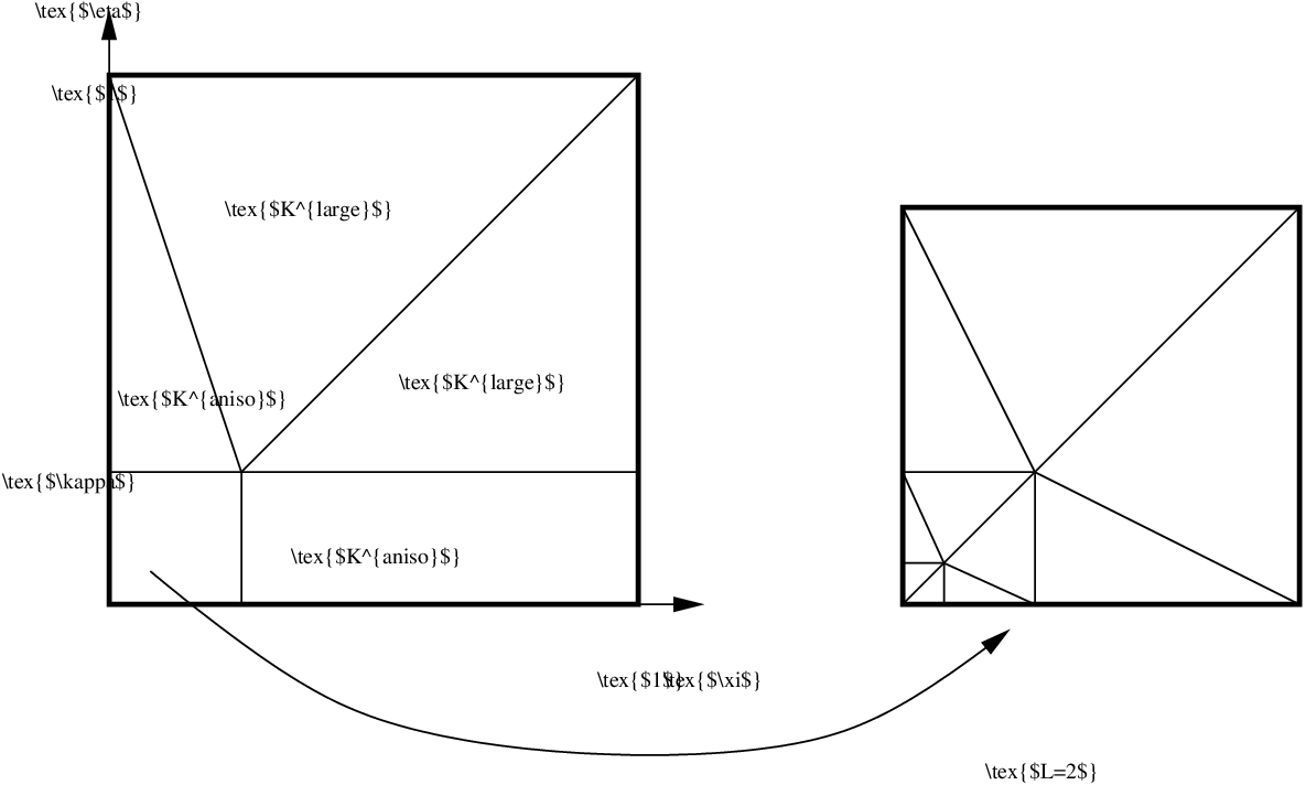
The tensor product patch: $\widehat{S}$ is split into at least four elements. The small square $(0,\kappa)^{2}$ may be further refined geometrically with $L\geq 0$ ( $L=0$ corresponds to no refinement) layers and a geometric grading factor $\sigma\in(0,1)$ ; see Fig. 1 (right). The triangulation of $\widehat{S}$ is decomposed into three types of elements: $\widehat{\mathcal{T}}^{large}$ consists of the one “large” element, $\widehat{\mathcal{T}}^{aniso}$ consists of the two anisotropic elements of aspect ratio $\mathcal{O}(1/\kappa)$ , and $\widehat{\mathcal{T}}^{CL}$ consists of the elements in $(0,\kappa)^{2}$ .
4.

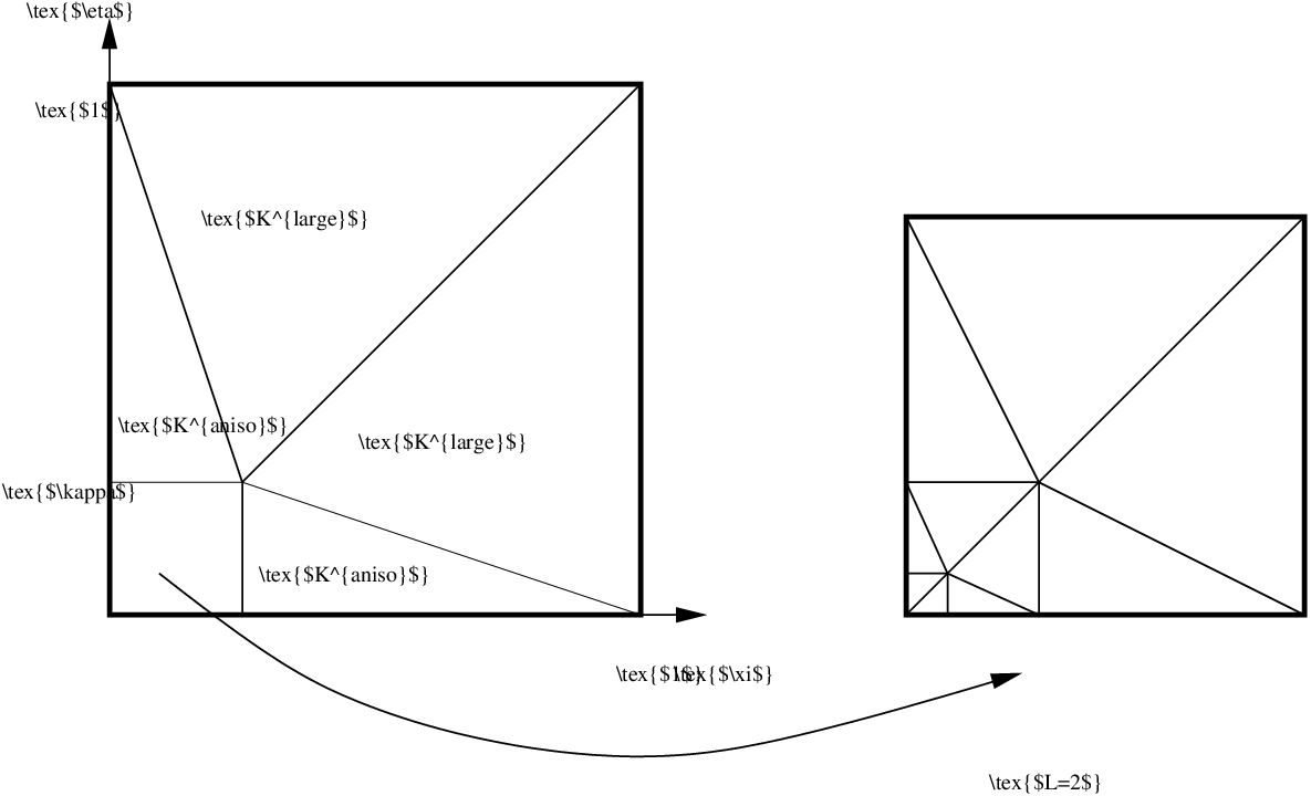
The mixed patches and the geometric patches: See Fig. 2. The triangulation is decomposed into three types of elements: $\widehat{\mathcal{T}}^{large}$ consists of the two “large” elements, $\widehat{\mathcal{T}}^{aniso}$ consists of the two anisotropic elements of aspect ratio $\mathcal{O}(1/\kappa)$ , and $\widehat{\mathcal{T}}^{CL}$ consists of the elements in $(0,\kappa)^{2}$ .

Since our analysis will mostly be done on the reference patterns, we introduce the notations $\widehat{\mathcal{T}}^{large}_{K^{\mathcal{M}}}$ , $\widehat{\mathcal{T}}^{aniso}_{K^{\mathcal{M}}}$ , $\widehat{\mathcal{T}}^{CL}_{K^{\mathcal{M}}}$ for the sets $\widehat{\mathcal{T}}^{large}$ , $\widehat{\mathcal{T}}^{aniso}$ , $\widehat{\mathcal{T}}^{CL}$ that correspond to the chosen refinement pattern for a macro-element $K^{\mathcal{M}}\in{\mathcal{T}}^{\mathcal{M}}$ .

Remark 3.2.

The list of admissible refinement patterns in Definition 3.1 is kept small in the interest of simplicity of exposition. A natural extension of the present list of patterns includes the case that all quadrilaterals of the refinement pattern are split into two triangles. The refinement patterns employed in the numerical example in Section 5 are also not included in Definition 3.1 but could be treated with the same techniques. In the same vein, the requirement 3 in Definition 3.3 below is imposed to shorten notation and to simplify the analysis. Furthermore, the stipulation that the macro-triangulation consist of quadrilaterals only could be relaxed to include triangles as well. Nevertheless, we point out that any triangulation consisting of triangles can be turned into one consisting of quadrilaterals by a suitable uniform refinement.

We consider meshes that result from applying these refinement patterns. Additionally, we impose further conditions on the choice of the refinement patterns for each element of the macro-triangulation:

Definition 3.3 (spectral boundary layer mesh ${\mathcal{T}}(\kappa,{\mathbf{L}})$ ).

Let ${\mathcal{T}}^{{\mathcal{M}}}$ be a fixed macro-triangulation consisting of quadrilaterals with analytic element maps that satisfies [6, Def. 2.4.1]. Fix $\sigma\in(0,1)$ and $\kappa\in(0,1/2]$ . For each macro-element $K^{{\mathcal{M}}}$ , select $L_{K^{{\mathcal{M}}}}\in{\mathbb{N}}_{0}$ and write ${\mathbf{L}}=(L_{K^{{\mathcal{M}}}})_{K^{{\mathcal{M}}}\in{\mathcal{T}}^{{\mathcal{M}}}}$ . A mesh ${\mathcal{T}}(\kappa,{\mathbf{L}})$ is called a spectral boundary layer mesh if the following conditions are satisfied:

1.

${\mathcal{T}}(\kappa,{\mathbf{L}})$ is obtained by refining each element $K^{{\mathcal{M}}}\in{\mathcal{T}}^{{\mathcal{M}}}$ according to one of the refinement patterns given in Definition 3.1 using the parameters $\sigma$ , $\kappa$ , and $L_{K^{{\mathcal{M}}}}$ .
2.

The resulting mesh ${\mathcal{T}}(\kappa,{\mathbf{L}})$ is a regular triangulation of $\Omega$ , i.e., it does not have hanging nodes. Since the element maps for the refinement patterns are assumed to be affine, this requirement ensures that the resulting triangulation satisfies [6, Def. 2.4.1].
3.

For each element $K^{{\mathcal{M}}}$ of the macro triangulation, we assume that for the intersection $\overline{K^{{\mathcal{M}}}}\cap\partial\Omega$ only the following cases can arise: a) it is empty; b) it consists of exactly one vertex; c) it consists of the closure of exactly one edge; d) it consists of the closure of exactly two edges intersecting at a corner of $\partial\Omega$ .

Further conditions on the choice of the refinement patterns are as follows:

4.

If exactly one edge $e$ of a macro-element $K^{{\mathcal{M}}}\in{\mathcal{T}}^{{\mathcal{M}}}$ lies on $\partial\Omega$ , then the corresponding reference edge $\widehat{e}=F^{-1}_{K^{\mathcal{M}}}(e)$ is $(0,1)\times\{0\}$ , and the refinement patterns of the boundary layer patch or the mixed patch is applied.
5.

If exactly two edges $e_{1}$ , $e_{2}$ of a macro-element $K^{{\mathcal{M}}}\in{\mathcal{T}}^{{\mathcal{M}}}$ lie on $\partial\Omega$ , then the corresponding reference edges are $(0,1)\times\{0\}$ and $\{0\}\times(0,1)$ , and the tensor product refinement pattern is applied.
6.

If exactly one vertex of a macro-element $K^{{\mathcal{M}}}\in{\mathcal{T}}^{{\mathcal{M}}}$ lies on $\partial\Omega$ , then the corresponding reference vertex is the point $(0,0)$ and the refinement pattern is either the tensor product patch, the mixed patch, or the geometric patch.

Refer to caption — Figure 1: Reference boundary layer patch (left); reference tensor product patch (right).

We refer the reader to Fig. 3 (right) for an example of a spectral boundary layer mesh.

The element maps $F_{K}:\widehat{K}\rightarrow K$ , $K\in{\mathcal{T}}(\kappa,{\mathbf{L}})$ , are given by the concatenation of affine maps from the reference square or triangle and the patch maps $F_{K^{{\mathcal{M}}}}$ . Here, the reference square is $(0,1)^{2}$ and the reference triangle $\{(x,y)\,|\,0<x<1,0<y<1-x\}$ . For any triangulation ${\mathcal{T}}$ we define $S^{p,1}({\mathcal{T}}):=\{u\in H^{1}(\Omega)\,|\,u|_{K}\circ F_{K}\in\Pi_{p}(\widehat{K})\}$ , where $\Pi_{p}(\widehat{K})$ is the tensor product space ${\mathcal{Q}}_{p}=\operatorname*{span}\{x^{i}y^{j}\,|\,0\leq i,j\leq p\}$ if $\widehat{K}=(0,1)^{2}$ and the space ${\mathcal{P}}_{p}=\operatorname*{span}\{x^{i}y^{j}\,|\,0\leq i+j\leq p\}$ if $\widehat{K}$ is the reference triangle. Finally, we set $S^{p,1}_{0}({\mathcal{T}}):=S^{p,1}({\mathcal{T}})\cap H^{1}_{0}(\Omega)$ .

A triangulation ${\mathcal{T}}(\kappa,{\mathbf{L}})$ has three types of elements that cover the regions $\Omega_{0}$ , $\Omega_{aniso}$ , and $\Omega_{CL}$ :

Definition 3.4 ( $\Omega_{0}$ , $\Omega_{aniso}$ , $\Omega_{CL}$ , ${\mathcal{V}}_{CL}$ ).

1.

The “large” elements ${\mathcal{T}}^{large}$ . These are the images (under the macro-element maps) of the trivial patch or the large elements (denoted $K^{large}$ in Figs. 1, 2). These elements are shape regular. We set $\Omega_{0}:=\left(\cup\{\overline{K_{i}}\,|\,K_{i}\in{\mathcal{T}}^{large}\}\right)^{\circ}$
2.

The “anisotropic elements” ${\mathcal{T}}^{aniso}$ . These elements are the images (under the macro-element maps) of elements of aspect ratio $\mathcal{O}(1/\kappa)$ , which are denoted by $K^{aniso}$ in Figs. 1, 2. We set $\Omega_{aniso}:=\left(\cup\{\overline{K_{i}}\,|\,K_{i}\in{\mathcal{T}}^{aniso}\}\right)^{\circ}$ .
3.

The “corner layer elements” ${\mathcal{T}}^{CL}$ : These elements are the images of elements in the $\mathcal{O}(\kappa)$ -neighborhood of $(0,0)$ of the reference pattern. These elements are shape regular. We set $\Omega_{CL}=\left(\cup\{\overline{K_{i}}\,|\,K_{i}\in{\mathcal{T}}^{CL}\}\right)^{\circ}$ .

${\mathcal{V}}_{CL}:=\{F_{K^{\mathcal{M}}}(0,0)\,|\,\mbox{$K^{\mathcal{M}}$ is either a tensor product or a mixed patch or geometric patch}\}$ denotes the set of vertices of the macro-triangulation towards which potentially geometric refinement is done.

Remark 3.5.

Key properties of the meshes ${\mathcal{T}}(\kappa,{\mathbf{L}})$ are: a) the elements abutting $\partial\Omega$ are either anisotropic or from $\Omega_{CL}$ ; b) geometric refinement can be ensured near the vertices of $\Omega$ ; c) there is $\mu>0$ (depending only on the macro-triangulation) such that

\operatorname*{dist}(\Omega_{0},\partial\Omega)\geq\mu\kappa.

(3.1)

In the notation of [6, Sec. 3.3.2], these meshes are patchwise structured meshes. In particular, therefore, the piecewise polynomial spaces $S^{p,1}_{0}({\mathcal{T}}(\kappa,{\mathbf{L}}))$ have approximation properties that were analyzed in [6, Sec. 3.4.2] and discussed in more detail in Proposition 3.9 below.

Remark 3.6.

(Scaling arguments) In our analysis, we will frequently appeal to scaling arguments. Strictly speaking, such arguments apply only to affine element maps. In the present case, the element maps are concatenations of affine maps and a fixed number of analytic diffeomorphisms (given by the element maps of the macro-triangulation). Hence, scaling arguments can be brought to bear for elements of the reference patterns on $\widehat{S}$ and then transplanted with the macro-element maps. In effect, therefore, scaling argument can be applied for estimates in $L^{2}$ and the $H^{1}$ -seminorm.

The following lemma constructs a lifting ${\mathcal{L}}_{0}$ as required in Section 2. ${\mathcal{L}}_{0}$ is controlled in the stronger norm $\|\cdot\|_{+}$ given by

\|{\mathcal{L}}_{0}\|\leq\|{\mathcal{L}}_{0}\|_{+}:=\sup_{v\in V_{N}\colon v|_{\partial\Omega_{0}}\neq 0}\frac{\|{\mathcal{L}}_{0}v\|_{L^{\infty}(\Omega)}+\varepsilon^{1/2}|{\mathcal{L}}_{0}v|_{H^{1}(\Omega\setminus\Omega_{0})}+\varepsilon^{-1/2}\|{\mathcal{L}}_{0}v\|_{L^{2}(\Omega\setminus\Omega_{0})}}{\|v\|_{L^{\infty}(\partial\Omega_{0})}}.

(3.2)

Lemma 3.7.

Let ${\mathcal{T}}(\kappa,{\mathbf{L}})$ be a spectral boundary layer mesh (Def. 3.3). Set $V_{N}:=S^{p,1}_{0}({\mathcal{T}}(\kappa,{\mathbf{L}}))$ . There exists a lifting operator ${\mathcal{L}}_{0}:V_{N}|_{\partial\Omega_{0}}\rightarrow V_{N}$ with

\displaystyle\|{\mathcal{L}}_{0}\|\leq\|{\mathcal{L}}_{0}\|_{+}

\displaystyle\leq C\left(p^{2}\frac{\varepsilon^{1/2}}{{\kappa^{1/2}}}+\frac{\kappa^{1/2}}{\varepsilon^{1/2}}\right).

(3.3)

The constant $C>0$ depends only on the shape-regularity of the macro-triangulation ${\mathcal{T}}^{{\mathcal{M}}}$ .

Proof.

The lifting ${\mathcal{L}}_{0}u$ is constructed patchwise, i.e., for each $K^{{\mathcal{M}}}\in{\mathcal{T}}^{{\mathcal{M}}}$ separately. To fix ideas, we construct the lifting for one refinement pattern only, namely, for a macro-element $K^{{\mathcal{M}}}$ that corresponds to the mixed patch of Fig. 2 (left). We use the vertices $\widehat{V}_{i}$ , $i=1,\ldots,8$ as shown in Fig. 3 (left). It is convenient to introduce $\partial\widehat{\Omega}_{0}:=F_{K^{{\mathcal{M}}}}^{-1}(\partial\Omega_{0}\cap\overline{K^{{\mathcal{M}}}})$ . This set consists of the union of the closure of edges and possibly single points. For the present case of the mixed patch it contains at least the two edges $\widehat{e}_{1}:=(\widehat{V}_{5},\widehat{V}_{6})$ and $\widehat{e}_{2}:=(\widehat{V}_{5},\widehat{V}_{7})$ . Let $u\in V_{N}|_{\partial{\Omega_{0}}}$ . We denote by $\widehat{u}$ the pull-back of $u$ to the reference configuration, i.e., $\widehat{u}:=u\circ F_{K^{{\mathcal{M}}}}$ , which is defined on $\partial\widehat{\Omega}_{0}$ . We now proceed to define the lifting ${\mathcal{L}}_{0}u$ by prescribing its extension $\widehat{\mathcal{L}}_{0}\widehat{u}$ on the reference patch. This is achieved in two steps: first, the values of $\widehat{\mathcal{L}}_{0}\widehat{u}$ are fixed on the edges of the macro-element; in a second step, the values of the edges are lifted to the elements. Let $V_{i}:=F_{K^{\mathcal{M}}}(\widehat{V}_{i})$ denote the image of $\widehat{V}_{i}$ under the patch map. We define $\widehat{\mathcal{L}}_{0}\widehat{u}$ in the nodes $\widehat{V}_{i}$ , $i=1,\ldots,7$ , as follows: If $V_{i}\in\partial{\Omega_{0}}$ , then $(\widehat{\mathcal{L}}_{0}\widehat{u})(\widehat{V}_{i}):=\widehat{u}(\widehat{V}_{i})=u(V_{i})$ . If $V_{i}\not\in\partial{\Omega_{0}}$ , then $(\widehat{\mathcal{L}}_{0}\widehat{u})(\widehat{V}_{i}):=0$ . Next, we define the values of $\widehat{\mathcal{L}}_{0}\widehat{u}$ on the $9$ edges given by $(\widehat{V}_{1},\widehat{V}_{2})$ , $(\widehat{V}_{2},\widehat{V}_{3})$ , $(\widehat{V}_{1},\widehat{V}_{4})$ , $(\widehat{V}_{4},\widehat{V}_{7})$ , $(\widehat{V}_{2},\widehat{V}_{5})$ , $(\widehat{V}_{4},\widehat{V}_{5})$ , $(\widehat{V}_{3},\widehat{V}_{6})$ , $(\widehat{V}_{6},\widehat{V}_{8})$ , $(\widehat{V}_{7},\widehat{V}_{8})$ . If the push-forward of an edge lies in $\partial{\Omega_{0}}$ , then $\widehat{\mathcal{L}}_{0}\widehat{u}$ is already defined by $\widehat{u}$ . If the push-forward does not lie in $\partial{\Omega_{0}}$ , then we let $\widehat{\mathcal{L}}_{0}\widehat{u}$ be the linear interpolant between the values at the endpoints (which we have defined above already). This defines $\widehat{\mathcal{L}}_{0}\widehat{u}$ in particular on the boundary $\partial(0,1)^{2}$ of the reference refinement pattern. Consider the case $L=0$ , i.e., the square $(0,\kappa)^{2}$ is not further refined. Then $\widehat{\mathcal{L}}_{0}\widehat{u}$ is already determined on all edges of the reference patch, and we can lift from the edges to the elements on which $\widehat{\mathcal{L}}_{0}\widehat{u}$ is still undefined. A fairly standard lifting, which we describe in Lemma A.1 for the reader’s convenience, ensures

\|\widehat{\mathcal{L}}_{0}\widehat{u}\|_{L^{\infty}(\widehat{S})}\leq C\max_{(x,y)\in\partial\widehat{\Omega}_{0}}|\widehat{u}(x,y)|,\qquad\|\nabla\widehat{\mathcal{L}}_{0}\widehat{u}\|_{L^{\infty}(\widehat{S})}\leq C\kappa^{-1}p^{2}\max_{(x,y)\in\partial\widehat{\Omega}_{0}}|\widehat{u}(x,y)|.

(3.4)

Here, the factor $\kappa^{-1}$ appears since the lifting is done on elements of aspect ratio $\mathcal{O}(1/\kappa)$ . We note that the thus defined function $\widehat{\mathcal{L}}_{0}\widehat{u}$ is also a continuous, piecewise polynomial of degree $p$ if the square $(0,\kappa)^{2}$ is refined geometrically with $L>0$ layers. Thus, we have constructed a lifting. Noting that $F_{K^{{\mathcal{M}}}}^{-1}(K^{{\mathcal{M}}}\setminus\Omega_{0})\subset(0,1)^{2}\setminus(\kappa,1)^{2}$ for the mixed patch, we infer

	$\displaystyle\\|{\mathcal{L}}_{0}u\\|_{L^{2}(K^{{\mathcal{M}}}\setminus\Omega_{0})}$	$\displaystyle\leq C\sqrt{\kappa}\max_{(x,y)\in\overline{K^{\mathcal{M}}}\cap\partial\Omega_{0}}\|u(x,y)\|,$
	$\displaystyle\\|\nabla{\mathcal{L}}_{0}u\\|_{L^{2}(K^{{\mathcal{M}}}\setminus\Omega_{0})}$	$\displaystyle\leq C\kappa^{-1/2}p^{2}\max_{(x,y)\in\overline{K^{\mathcal{M}}}\cap\partial\Omega_{0}}\|u(x,y)\|.$

In this way, we construct the lifting for each refinement pattern and consequently patch by patch. It is essential to note that our assumptions on the refinement patterns are such that the patchwise defined lifting is continuous across patch boundaries, i.e., it is actually in $S^{p,1}_{0}({\mathcal{T}}(\kappa,{\mathbf{L}}))$ . ∎

We will also need a second lifting operator:

Lemma 3.8.

There is a lifting ${\mathcal{L}}_{CL}:V_{N}|_{\partial\Omega_{CL}}\rightarrow V_{N}$ with the following property:

\displaystyle\|{\mathcal{L}}_{CL}\|:=\!\!\sup_{v\in V_{N}:v|_{\partial\Omega_{CL}}\neq 0}\!\!\frac{|{\mathcal{L}}_{CL}v|_{H^{1}(\Omega_{CL})}+\varepsilon^{-1}\|{\mathcal{L}}_{CL}v\|_{L^{2}(\Omega_{CL})}+\|{\mathcal{L}}_{CL}v\|_{L^{\infty}(\Omega_{CL})}}{\|v\|_{L^{\infty}(\partial\Omega_{CL})}}\leq C\left[p^{2}+\frac{\kappa}{\varepsilon}\right].

(3.5)

Proof.

The lifting is again constructed patchwise. For simplicity, we will not construct the lifting to $\Omega$ but only to $\Omega_{CL}$ , since we are only interested in $({\mathcal{L}}_{CL}u)|_{\Omega_{CL}}$ .

We observe that $\Omega_{CL}$ is the union of images of the square $(0,\kappa)^{2}$ under certain macro-element maps and that push-forwards of the lines $\widehat{e}_{1}:=(0,\kappa)\times\{\kappa\}$ and $\widehat{e}_{2}:=\{\kappa\}\times(0,\kappa)$ form part of the boundary of $\Omega_{CL}$ . The remaining two lines $\widehat{e}_{3}:=(0,\kappa)\times\{0\}$ and $\widehat{e}_{4}:=\{0\}\times(0,\kappa)$ are either mapped to subsets of $\partial\Omega$ or are meshlines that are completely inside $\Omega_{CL}$ . On $(0,\kappa)^{2}$ we define ${\mathcal{L}}_{CL}$ as follows: Let $u\in V_{N}|_{\partial\Omega_{CL}}$ and $\widehat{u}$ be its pull-back under the macro-element map $F_{K^{\mathcal{M}}}$ . Fix $\widehat{\mathcal{L}}_{CL}\widehat{u}$ to coincide with $\widehat{u}$ on the lines $\widehat{e}_{1}$ and $\widehat{e}_{2}$ , to be zero in $(0,0)$ , and to be the linear interpolant on the remaining two edges $\widehat{e}_{3}$ and $\widehat{e}_{4}$ . Finally, $\widehat{\mathcal{L}}_{CL}\widehat{u}$ is lifted to $(0,\kappa)^{2}$ by a standard lifting, e.g., the one constructed in Lemma A.1. We conclude

\|\widehat{\mathcal{L}}_{CL}\widehat{u}\|_{L^{\infty}((0,\kappa)^{2})}+p^{-2}\kappa\|\nabla\widehat{\mathcal{L}}_{CL}\widehat{u}\|_{L^{\infty}((0,\kappa)^{2})}\lesssim\|\widehat{u}\|_{L^{\infty}(\widehat{e}_{1}\cup\widehat{e}_{2})}.

(3.6)

Transforming to $F_{K^{\mathcal{M}}}((0,\kappa)^{2})$ yields (3.5). ∎

By selecting $\kappa={\mathcal{O}}(p\varepsilon)$ in the spectral boundary layer meshes ${\mathcal{T}}(\kappa,{\mathbf{L}})$ , one can construct an approximation $\Pi u\in S^{p,1}_{0}({\mathcal{T}}(\kappa,{\mathbf{L}}))$ with the following approximation properties:

Proposition 3.9.

For parameters $\lambda>0$ and polynomial degrees $p$ consider meshes ${\mathcal{T}}(\min\{\lambda p\varepsilon,1/2\},{\mathbf{L}})$ . Let $L$ be defined as $L:=\min\{{L}_{K^{\mathcal{M}}}\,|\,K^{{\mathcal{M}}}\,\text{s.t.}\,F_{K^{\mathcal{M}}}(0,0)\,\text{is a vertex of }\,\Omega\}$ . Then, there exist $\lambda_{0}>0$ , $b$ , $C>0$ depending only on $\Omega$ , $A$ , $c$ , and $f$ such that the following is true: For every $\lambda\in(0,\lambda_{0}]$ there exists an approximation $\Pi u\in S^{p,1}_{0}({\mathcal{T}}(\min\{\lambda p\varepsilon,1/2\},{\mathbf{L}}))$ such that


$\displaystyle\\|u-\Pi u\\|_{L^{\infty}(\Omega)}$	$\displaystyle\leq Cp^{4}\left(\lambda^{-1/2}e^{-b\lambda p}+pe^{-bL}\right),$	(3.7a)
$\displaystyle\\|u-\Pi u\\|_{L^{\infty}(\Omega\setminus\Omega_{CL})}$	$\displaystyle\leq Cp^{4}\lambda^{-1/2}e^{-b\lambda p},$	(3.7b)
$\displaystyle\varepsilon^{1/2}\\|\nabla(u-\Pi u)\\|_{L^{2}(\Omega)}$	$\displaystyle\leq Cp^{4}\left(\lambda^{-1/2}e^{-b\lambda p}+\sqrt{\varepsilon}p^{2}e^{-bL}\right).$	(3.7c)

Furthermore, for arbitrary $\overline{x}\in{\mathbb{R}}^{2}$ we have

	$\displaystyle\\|\nabla(u-\Pi u)\\|_{L^{2}(B_{\lambda p\varepsilon}(\overline{x})\cap\Omega_{CL})}$	$\displaystyle\leq Cp^{4}\left(\lambda^{-1/2}e^{-b\lambda p}+p^{2}e^{-bL}\right),$		(3.8)
	$\displaystyle\\|\nabla(u-\Pi u)\\|_{L^{2}(B_{\lambda p\varepsilon}(\overline{x})\cap(\Omega\backslash\Omega_{CL}))}$	$\displaystyle\leq Cp^{4}\lambda^{-1/2}e^{-b\lambda p}.$		(3.9)

Proof.

The result relies on a careful inspection of [6, Thm. 3.4.8] and a modification of the boundary layer approximation that goes back to [14] for the 1D case (see also [7]). Of interest to us and in our tracking of the procedure in [6, Thm. 3.4.8] is the case that $\lambda p\varepsilon$ is sufficiently small, since in the case $\lambda p\varepsilon\gtrsim 1$ , we may estimate $\varepsilon^{-1}\lesssim\lambda p$ and absorb powers of $\lambda p$ in the exponentially decaying term $e^{-b\lambda p}$ . It is also that regime that is responsible for the factor $\sqrt{\varepsilon}p^{2}e^{-bL}$ instead of a factor $\sqrt{\varepsilon}pe^{-bL}$ in (3.7c). We emphasize that in the course of the proof, the constants $C$ , $b>0$ may be different in each occurrence. We also mention that the factor $p^{4}$ results from simply estimating $p^{3}(1+\ln p)\lesssim p^{4}$ .

Let $\Pi^{\infty}_{p,{\mathcal{T}}}$ be the approximation operator employed in the proof of [6, Thm. 3.4.8]. This operator has the following stability properties by [6, Thm. 3.2.20]: Its pull-back $\Pi^{\infty}_{p,\widehat{K}}$ to the reference element $\widehat{K}$ (which can be either the reference triangle or the reference square) satisfies

		$\displaystyle(\Pi^{\infty}_{p,\widehat{K}}v)\|_{e}\quad\mbox{ coincides with the Gauss-Lobatto interpolant of $v\|_{e}$ on each edge $e$ of $\widehat{K}$},$		(3.10)
		$\displaystyle\\|v-\Pi^{\infty}_{p,\widehat{K}}v\\|_{L^{\infty}(\widehat{K})}\lesssim C_{p}\inf_{w\in\Pi_{p}(\widehat{K})}\\|v-w\\|_{L^{\infty}(\widehat{K})},\qquad C_{p}:=p(1+\ln p),$		(3.11)
		$\displaystyle\\|\nabla(v-\Pi^{\infty}_{p,\widehat{K}}v)\\|_{L^{2}(\widehat{K})}\lesssim\inf_{w\in\Pi_{p}(\widehat{K})}\\|\nabla(v-w)\\|_{L^{2}(\widehat{K})}+p^{2}C_{p}\\|v-w\\|_{L^{\infty}(\widehat{K})}.$		(3.12)

We inspect the proof of [6, Thm. 3.4.8], which studies $u-\Pi^{\infty}_{p,{\mathcal{T}}}u$ , and modify as needed. The exact solution $u$ of (1.1) is written as $u=w_{\varepsilon}+\chi^{BL}u^{BL}_{\varepsilon}+\chi^{CL}u^{CL}_{\varepsilon}+r_{\varepsilon}$ , where $w_{\varepsilon}$ represents the smooth part of an asymptotic expansion, $u^{BL}_{\varepsilon}$ the boundary layer part, $u^{CL}_{\varepsilon}$ the corner layer and $r_{\varepsilon}$ the (exponentially small) remainder; the smooth cut-off functions $\chi^{BL}$ , $\chi^{CL}$ localize near $\partial\Omega$ and the vertices of $\Omega$ , respectively. (The properties of $w_{\varepsilon}$ , $r_{\varepsilon}$ , $u^{BL}_{\varepsilon}$ , $u^{CL}_{\varepsilon}$ are detailed in [6, Thm. 2.3.4].) The desired approximation $\Pi u$ will be constructed of the form

\Pi u=\Pi^{\infty}_{p,{\mathcal{T}}}w_{\varepsilon}+\Pi^{\infty}_{p,{\mathcal{T}}}r_{\varepsilon}+\Pi^{BL}\chi^{BL}u^{BL}_{\varepsilon}+\Pi^{CL}\chi^{CL}u^{CL}_{\varepsilon}.

(3.13)

We analyze these $4$ terms in turn.

Treatment of $w_{\varepsilon}$ : The function $w_{\varepsilon}$ is analytic with $\|\nabla^{n}w_{\varepsilon}\|_{L^{\infty}(\Omega)}\leq C\gamma^{n}n!\quad\forall n\in{\mathbb{N}}_{0}$ with constants $C$ , $\gamma>0$ independent of $\varepsilon$ . This implies for the shape-regular elements $K\in{\mathcal{T}}^{large}\cup{\mathcal{T}}^{CL}$ with $h_{K}$ denoting the element diameter

h_{K}^{-1}\|w_{\varepsilon}-\Pi^{\infty}_{p,{\mathcal{T}}}w_{\varepsilon}\|_{L^{\infty}(K)}+\|\nabla(w_{\varepsilon}-\Pi^{\infty}_{p,{\mathcal{T}}}w_{\varepsilon})\|_{L^{\infty}(K)}\leq Ce^{-bp}.

(3.14)

For the anisotropic elements $K\in{\mathcal{T}}^{aniso}$ , we get

\|w_{\varepsilon}-\Pi^{\infty}_{p,{\mathcal{T}}}w_{\varepsilon}\|_{L^{\infty}(K)}+\kappa\|\nabla(w_{\varepsilon}-\Pi^{\infty}_{p,{\mathcal{T}}}w_{\varepsilon})\|_{L^{\infty}(K)}\leq Ce^{-bp}.

(3.15)

Since $\kappa=\lambda p\varepsilon$ , the estimates (3.14), (3.15) provide the desired estimates for the contribution of $w_{\varepsilon}$ .

Treatment of $r_{\varepsilon}$ : [6, Thm. 2.3.4] gives $\|r_{\varepsilon}\|_{L^{\infty}(\Omega)}+\|r_{\varepsilon}\|_{H^{1}(\Omega)}\lesssim e^{-b/\varepsilon}$ . (3.11), (3.12), the fact that elements have aspect ratio at most ${\mathcal{O}}(1/(\lambda p\varepsilon))$ and the assumption $\lambda p\varepsilon\lesssim 1$ imply (cf. also the arguments leading to [6, (3.4.25)–(3.4.27)])

\|r_{\varepsilon}-\Pi^{\infty}_{p,{\mathcal{T}}}r_{\varepsilon}\|_{L^{\infty}(\Omega)}+\sqrt{\lambda p\varepsilon}\|\nabla(r_{\varepsilon}-\Pi^{\infty}_{p,{\mathcal{T}}}r_{\varepsilon})\|_{L^{2}(\Omega)}\leq Cp^{2}C_{p}e^{-b/\varepsilon}\leq Cp^{2}C_{p}e^{-b\lambda p}.

(3.16)

Since $\varepsilon\lesssim 1/(\lambda p)$ this last inequality implies additionally

\|\nabla(r_{\varepsilon}-\Pi^{\infty}_{p,{\mathcal{T}}}r_{\varepsilon})\|_{L^{2}(\Omega)}\lesssim\frac{1}{(\lambda p\varepsilon)^{1/2}}p^{2}C_{p}e^{-b/\varepsilon}\lesssim\frac{1}{\lambda^{1/2}}p^{3/2}C_{p}e^{-b/\varepsilon}\lesssim\frac{1}{\lambda^{1/2}}p^{3/2}C_{p}e^{-b\lambda p}.

(3.17)

These estimates provide the desired estimates for the contribution of $r_{\varepsilon}$ .

Treatment of $\chi^{BL}u^{BL}_{\varepsilon}$ : From [6, (3.4.28)] we get for the boundary layer part $\chi^{BL}u^{BL}_{\varepsilon}$

\|\chi^{BL}u^{BL}_{\varepsilon}-\Pi^{\infty}_{p,{\mathcal{T}}}\chi^{BL}u^{BL}_{\varepsilon}\|_{L^{\infty}(\Omega)}+\lambda p\varepsilon\|\nabla(\chi^{BL}u^{BL}_{\varepsilon}-\Pi^{\infty}_{p,{\mathcal{T}}}\chi^{BL}u^{BL}_{\varepsilon})\|_{L^{\infty}(\Omega)}\lesssim C_{p}p^{2}e^{-b\lambda p}.

(3.18)

The approximation $\Pi^{\infty}_{p,{\mathcal{T}}}\chi^{BL}u^{BL}_{\varepsilon}$ needs to be corrected in the spirit of [14] in order to control $\varepsilon^{1/2}\|\nabla(u-\Pi u)\|_{L^{2}(\Omega)}$ . Specifically, we approximate $\chi^{BL}u^{BL}_{\varepsilon}$ by

\Pi^{BL}\chi^{BL}u^{BL}_{\varepsilon}:=\begin{cases}0&x\in\Omega_{0}\\ \Pi^{\infty}_{p,{\mathcal{T}}}\chi^{BL}u^{BL}_{\varepsilon}-{\mathcal{L}}_{0}\left(\Pi^{\infty}_{p,{\mathcal{T}}}\chi^{BL}u^{BL}_{\varepsilon}\right)&x\in\Omega\setminus\Omega_{0},\end{cases}

(3.19)

where ${\mathcal{L}}_{0}$ is the lifting operator of Lemma 3.7. Note that $(\Pi^{BL}\chi^{BL}u^{BL}_{\varepsilon})|_{\partial\Omega}=\Pi^{\infty}_{p,{\mathcal{T}}}\chi^{BL}u^{BL}_{\varepsilon}$ . For the analysis of the approximation properties of $\Pi^{BL}\chi^{BL}u^{BL}_{\varepsilon}$ , we introduce the shorthand notation

\widetilde{u}^{BL}:=\chi^{BL}u^{BL}_{\varepsilon}\qquad\mbox{ and }\qquad\widetilde{u}^{BL}_{p}:=\Pi^{\infty}_{p,{\mathcal{T}}}(\chi^{BL}u^{BL}_{\varepsilon}).

We use that $\operatorname*{dist}(\Omega_{0},\partial\Omega)\geq\mu\lambda p\varepsilon$ for some $\mu>0$ (cf. (3.1)). The decay properties of the boundary layer (cf. [6, Thm. 2.3.4]) then read

\varepsilon^{-1/2}\|\widetilde{u}^{BL}\|_{L^{2}(\Omega_{0})}+\varepsilon^{1/2}\|\nabla\widetilde{u}^{BL}\|_{L^{2}(\Omega_{0})}+\|\widetilde{u}^{BL}\|_{L^{\infty}(\Omega_{0})}+\varepsilon\|\nabla\widetilde{u}^{BL}\|_{L^{\infty}(\Omega_{0})}\lesssim e^{-b\lambda p}.

(3.20)

These estimates and the fact $\|\cdot\|_{L^{2}(B_{\lambda p\varepsilon}(\overline{x})\cap\Omega_{0})}\lesssim\lambda p\varepsilon\|\cdot\|_{L^{\infty}(B_{\lambda p\varepsilon}(\overline{x})\cap\Omega_{0})}$ produce the correct estimates for the approximation of $\chi^{BL}u^{BL}_{\varepsilon}$ on $\Omega_{0}$ .

In order to analyze the error on $\Omega\setminus\Omega_{0}$ we need to control $\Pi^{\infty}_{p,{\mathcal{T}}}(\chi^{BL}u^{BL}_{\varepsilon})$ on $\partial\Omega_{0}$ . To that end, we note that the stability properties of $\Pi^{\infty}_{p,{\mathcal{T}}}$ given in (3.11) and the fact that the elements in $\Omega_{0}$ are shape-regular and of size ${\mathcal{O}}(1)$ imply

\displaystyle\|\widetilde{u}^{BL}_{p}\|_{L^{\infty}(\Omega_{0})}

\displaystyle\lesssim C_{p}\|\widetilde{u}^{BL}\|_{L^{\infty}(\Omega_{0})}\lesssim C_{p}e^{-b\lambda p}.

(3.21)

By construction, we have on $\Omega\setminus\Omega_{0}$

\widetilde{u}^{BL}-\Pi^{BL}(\chi^{BL}u^{BL}_{\varepsilon})=\widetilde{u}^{BL}-\widetilde{u}^{BL}_{p}+{\mathcal{L}}_{0}\widetilde{u}^{BL}_{p}.

Since $\operatorname*{meas}(\Omega\setminus\Omega_{0})=\mathcal{O}(\lambda p\varepsilon)$ and $\|{\cdot}\|_{L^{2}(\Omega\backslash\Omega_{0})}\lesssim\operatorname*{meas}(\Omega\setminus\Omega_{0})^{1/2}\|{\cdot}\|_{L^{\infty}(\Omega\backslash\Omega_{0})}$ , we get from (3.18) the following estimates for the first term $\widetilde{u}^{BL}-\widetilde{u}^{BL}_{p}$ :

\displaystyle(\lambda p\varepsilon)^{-1/2}\|\widetilde{u}^{BL}-\widetilde{u}^{BL}_{p}\|_{L^{2}(\Omega\setminus\Omega_{0})}+(\lambda p\varepsilon)^{1/2}\|\nabla(\widetilde{u}^{BL}-\widetilde{u}^{BL}_{p})\|_{L^{2}(\Omega\setminus\Omega_{0})}\lesssim C_{p}p^{2}e^{-b\lambda p}.

(3.22)

For the term ${\mathcal{L}}_{0}\widetilde{u}^{BL}_{p}$ , we use the estimates of Lemma 3.7 and (3.21) to arrive at

	$\displaystyle\varepsilon^{1/2}\\|\nabla{\mathcal{L}}_{0}\widetilde{u}^{BL}_{p}\\|_{L^{2}(\Omega\setminus\Omega_{0})}+\varepsilon^{-1/2}\\|{\mathcal{L}}_{0}\widetilde{u}^{BL}_{p}\\|_{L^{2}(\Omega\setminus\Omega_{0})}+\\|{\mathcal{L}}_{0}\widetilde{u}^{BL}_{p}\\|_{L^{\infty}(\Omega)}$	$\displaystyle\leq\\|{\mathcal{L}}_{0}\\|\\|\widetilde{u}^{BL}_{p}\\|_{L^{\infty}(\partial\Omega_{0})}$
		$\displaystyle\leq Cp^{3/2}\lambda^{-1/2}C_{p}e^{-b\lambda p}.$		(3.23)

As in the proof of Lemma 3.7 (cf. (3.4)), we obtain, since $\operatorname*{meas}(B_{\lambda p\varepsilon}(\overline{x}))=\mathcal{O}((\lambda p\varepsilon)^{2})$ ,

\|\nabla{\mathcal{L}}_{0}\widetilde{u}^{BL}_{p}\|_{L^{2}(B_{\lambda p\varepsilon}(\overline{x})\cap(\Omega\setminus\Omega_{0}))}\lesssim\lambda\varepsilon p\|\nabla{\mathcal{L}}_{0}\widetilde{u}^{BL}_{p}\|_{L^{\infty}(B_{\lambda p\varepsilon}(\overline{x})\cap(\Omega\setminus\Omega_{0}))}\lesssim p^{2}\|\widetilde{u}^{BL}_{p}\|_{L^{\infty}(\partial\Omega_{0})}\leq Cp^{2}C_{p}e^{-b\lambda p},

which allows us to conclude that the approximation $\Pi^{BL}(\chi^{BL}u^{BL}_{\varepsilon})$ has the desired properties.

Treatment of $u^{CL}_{\varepsilon}$ : Finally, for the corner layer contribution we use [6, (3.4.29)—(3.4.33)]. Again, we abbreviate

\widetilde{u}^{CL}:=\chi^{CL}u^{CL}_{\varepsilon},\qquad\mbox{ and }\qquad\widetilde{u}^{CL}_{p}=\Pi^{\infty}_{p,{\mathcal{T}}}(\chi^{CL}u^{CL}_{\varepsilon}).

We infer directly from [6, (3.4.33)]:

\displaystyle\|\widetilde{u}^{CL}-\widetilde{u}^{CL}_{p}\|_{L^{\infty}(\Omega_{CL})}+\|\nabla(\widetilde{u}^{CL}-\widetilde{u}^{CL}_{p})\|_{L^{2}(\Omega_{CL})}

\displaystyle\lesssim C_{p}p^{3}e^{-bL}+e^{-bp}.

(3.24)

As in our treatment of the boundary layer part, we need to modify the approximation $\Pi^{\infty}_{p,{\mathcal{T}}}\chi^{CL}u^{CL}_{\varepsilon}$ . We set

\Pi^{CL}\chi^{CL}u^{CL}_{\varepsilon}:=\begin{cases}0&x\in\Omega\setminus\Omega_{CL}\\ \Pi^{\infty}_{p,{\mathcal{T}}}\chi^{CL}u^{CL}_{\varepsilon}-{\mathcal{L}}_{CL}\left(\Pi^{\infty}_{p,{\mathcal{T}}}\chi^{CL}u^{CL}_{\varepsilon}\right)&x\in\Omega_{CL},\end{cases}

(3.25)

where ${\mathcal{L}}_{CL}$ is the lifting operator of Lemma 3.8. Note that $(\Pi^{CL}\chi^{CL}u^{CL}_{\varepsilon})|_{\partial\Omega}=\Pi^{\infty}_{p,{\mathcal{T}}}\chi^{CL}u^{CL}_{\varepsilon}$ .

The decay properties of the corner layer (cf. [6, Thm. 2.3.4]) then read

\varepsilon^{-1}\|\widetilde{u}^{CL}\|_{L^{2}(\Omega\setminus\Omega_{CL})}+\|\nabla\widetilde{u}^{CL}\|_{L^{2}(\Omega\setminus\Omega_{CL})}+\|\widetilde{u}^{CL}\|_{L^{\infty}(\Omega\setminus\Omega_{CL})}+\varepsilon\|\nabla\widetilde{u}^{CL}\|_{L^{\infty}(\Omega\setminus\Omega_{CL})}\lesssim e^{-b\lambda p}.

(3.26)

These estimates imply that our approximation of the corner layer contribution has the desired properties on $\Omega\setminus\Omega_{CL}$ .

The stability properties of $\Pi^{\infty}_{p,{\mathcal{T}}}$ yield

\displaystyle\|\widetilde{u}^{CL}_{p}\|_{L^{\infty}(\Omega\setminus\Omega_{CL})}

\displaystyle\lesssim C_{p}\|\widetilde{u}^{CL}\|_{L^{\infty}(\Omega\setminus\Omega_{CL})}\lesssim C_{p}e^{-b\lambda p}.

(3.27)

By construction we have on $\Omega_{CL}$

\chi^{CL}u^{CL}_{\varepsilon}-\Pi^{CL}(\chi^{CL}u^{CL}_{\varepsilon})=\widetilde{u}^{CL}-\widetilde{u}^{CL}_{p}+{\mathcal{L}}_{CL}\widetilde{u}^{CL}_{p}.

The estimates of (3.24) give the desired bounds for the contribution $\widetilde{u}^{CL}-\widetilde{u}^{CL}_{p}$ . For the correction ${\mathcal{L}}_{CL}\widetilde{u}^{CL}_{p}$ we use Lemma 3.8 and the bound (3.27) to get

	$\displaystyle\\|\nabla{\mathcal{L}}_{CL}\widetilde{u}^{CL}_{p}\\|_{L^{2}(\Omega_{CL})}+\varepsilon^{-1}\\|{\mathcal{L}}_{CL}\widetilde{u}^{CL}_{p}\\|_{L^{2}(\Omega_{CL})}+\\|{\mathcal{L}}_{CL}\widetilde{u}^{CL}_{p}\\|_{L^{\infty}(\Omega_{CL})}$	$\displaystyle\lesssim\\|{\mathcal{L}}_{CL}\\|\\|\widetilde{u}^{CL}_{p}\\|_{L^{\infty}(\partial\Omega_{CL})}$
		$\displaystyle\lesssim C_{p}p^{2}e^{-b\lambda p}.\qed$

Theorem 3.10.

Assume the hypotheses of Proposition 3.9 and let $\lambda_{0}$ , which depends solely on $\Omega$ , $A$ , $c$ , and $f$ , be given by Proposition 3.9. Then for each $\lambda\in(0,\lambda_{0}]$ there exist $C$ , $b>0$ independent of $p$ and $\varepsilon$ such that for the solution $u$ of (1.1) and its Galerkin approximation $u_{N}\in S^{p,1}_{0}({\mathcal{T}}(\min\{\lambda p\varepsilon,1/2\},{\mathbf{L}}))$ there holds

\|u-u_{N}\|_{\sqrt{\varepsilon}}\leq C\left(e^{-bp}+\sqrt{\varepsilon}p^{6}e^{-bL}\right).

Proof.

With $\Pi u$ of Proposition 3.9, the $L^{\infty}$ -estimates of Proposition 3.9 applied on $\Omega\backslash\Omega_{CL}$ and on $\Omega_{CL}$ together with $\operatorname*{meas}(\Omega_{CL})={\mathcal{O}}((p\varepsilon)^{2})$ , we have

\|u-u_{N}\|_{L^{2}(\Omega)}\leq\|u-u_{N}\|_{\varepsilon}\leq\inf_{v\in V_{N}}\|u-v\|_{\varepsilon}\leq\|u-\Pi u\|_{\varepsilon}\leq Cp^{4}\left(e^{-bp}+\sqrt{\varepsilon}p^{2}e^{-bL}\right).

(3.28)

We are therefore left with estimating $|u-u_{N}|_{\sqrt{\varepsilon}}$ . To that end, we apply Corollary 2.3 with $v=\Pi u$ of Proposition 3.9, which yields, since $\operatorname*{meas}(\Omega\setminus(\Omega_{0}\cup\Omega_{CL}))={\mathcal{O}}(p\varepsilon)$ and $\operatorname*{meas}(\Omega_{CL})={\mathcal{O}}((p\varepsilon)^{2})$

\displaystyle|u-u_{N}|_{\sqrt{\varepsilon}}

\displaystyle\lesssim\|{\mathcal{L}}_{0}\|\|\Pi^{L^{2}}_{\Omega_{0}}u-\Pi u\|_{L^{\infty}(\partial\Omega_{0})}+\sqrt{\varepsilon}\|\nabla(\Pi^{L^{2}}_{\Omega_{0}}u-\Pi u)\|_{L^{2}(\Omega_{0})}+p^{4.5}e^{-bp}+\sqrt{\varepsilon}p^{6}e^{-bL}.

We exploit that $\Omega_{0}$ consists of a fixed number of shape-regular elements. Hence, a polynomial inverse estimate on the reference element (cf. [13, (4.6.5)]) gives, since $\Omega_{0}\cap\Omega_{CL}=\emptyset$ ,

\|\nabla(\Pi^{L^{2}}_{\Omega_{0}}u-\Pi u)\|_{L^{2}(\Omega_{0})}\lesssim p^{2}\|\Pi^{L^{2}}_{\Omega_{0}}u-\Pi u\|_{L^{2}(\Omega_{0})}\lesssim p^{2}\|u-\Pi u\|_{L^{2}(\Omega_{0})}\lesssim p^{6}e^{-bp}.

The term $\|\Pi^{L^{2}}_{\Omega_{0}}u-\Pi u\|_{L^{\infty}(\partial\Omega_{0})}$ is estimated again with polynomial inverse estimates (cf. [13, (4.6.1)])

	$\displaystyle\\|\Pi^{L^{2}}_{\Omega_{0}}u-\Pi u\\|_{L^{\infty}(\partial\Omega_{0})}\leq\\|\Pi^{L^{2}}_{\Omega_{0}}u-\Pi u\\|_{L^{\infty}(\Omega_{0})}\lesssim p^{2}\\|\Pi^{L^{2}}_{\Omega_{0}}u-\Pi u\\|_{L^{2}(\Omega_{0})}$	$\displaystyle\lesssim p^{2}\\|u-\Pi u\\|_{L^{2}(\Omega_{0})}$
		$\displaystyle\lesssim p^{6}e^{-bp}.$

Finally, Lemma 3.7 yields $\|{\mathcal{L}}_{0}\|\leq Cp^{3/2}$ for fixed $\lambda$ . ∎

4 $L^{\infty}$ -estimates

$L^{\infty}$ -estimates for the Galerkin error $u-u_{N}$ are obtained in $3$ steps: using the fact that the number of elements in $\Omega_{0}$ and in $\Omega_{aniso}$ is fixed, we estimate first $\|u-u_{N}\|_{L^{\infty}(\Omega_{0})}$ and then $\|u-u_{N}\|_{L^{\infty}(\Omega_{aniso})}$ . In a final step, we estimate $\|u-u_{N}\|_{L^{\infty}(\Omega_{CL})}$ . For this last estimate, we need to make an assumption on the vector ${\mathbf{L}}$ , namely, that significant geometric refinement is only possible at the boundary $\partial\Omega$ :

Assumption 4.1.

There is $L_{\infty}\geq 0$ such that for each $K^{\mathcal{M}}$ with $V:=F_{K^{\mathcal{M}}}(0,0)\in{\mathcal{V}}_{CL}$ the following dichotomy holds: either ( $V\in\Omega$ and $L_{K^{\mathcal{M}}}\leq L_{\infty}$ ) or $V\in\partial\Omega$ .

Lemma 4.2.

Let $V_{N}\subset H^{1}_{0}(\Omega)$ be a closed subspace. Let $\widetilde{\Omega}_{0}\subset\Omega$ be open. Let $u\in H^{1}_{0}(\Omega)$ and $u_{N}\in V_{N}$ satisfy the Galerkin orthogonality (2.1). Let $Iu\in V_{N}$ satisfy $Iu|_{\widetilde{\Omega}_{0}}=u_{N}|_{\widetilde{\Omega}_{0}}$ . Then, for an implied constant depending solely on $\|A\|_{L^{\infty}(\Omega)}$ , $\|c\|_{L^{\infty}(\Omega)}$ , $\alpha_{0}$ , $c_{0}$ there holds

|u_{N}-Iu|_{H^{1}(\Omega\setminus\widetilde{\Omega}_{0})}\lesssim|u-Iu|_{H^{1}(\Omega\setminus\widetilde{\Omega}_{0})}+\varepsilon^{-1}\|u-Iu\|_{L^{2}(\Omega\setminus\widetilde{\Omega}_{0})}.

(4.1)

Proof.

Proceeds as in the proof of Lemma 2.1. ∎

Lemma 4.3.

Let Assumption 4.1 be valid. Let $V_{N}:=S^{p,1}_{0}({\mathcal{T}}(\kappa,{\mathbf{L}}))$ . Let $u_{N}$ , $Iu\in V_{N}$ satisfy $(u_{N}-Iu)|_{\partial\Omega_{CL}}=0$ . Then

\|u_{N}-Iu\|_{L^{\infty}(\Omega_{CL})}\leq Cp\|\nabla(u_{N}-Iu)\|_{L^{2}(\Omega_{CL})}.

(4.2)

The constant $C>0$ depends only on the shape-regularity properties of ${\mathcal{T}}^{\mathcal{M}}$ .

Proof.

We note

\Omega_{CL}=\left(\bigcup_{V\in{\mathcal{V}}_{CL}}\bigcup\left\{F_{K^{\mathcal{M}}}([0,\kappa]^{2})\,|\,\mbox{$K^{\mathcal{M}}\in{\mathcal{T}}^{\mathcal{M}}$ such that $F_{K^{\mathcal{M}}}(0,0)=V$}\right\}\right)^{\circ}.

Consider a fixed $V\in{\mathcal{V}}_{CL}$ . The cases $V\in\Omega$ or $V\in\partial\Omega$ may occur.

The case $V\in\Omega$ : Assumption 4.1 implies that any macro-element $K^{\mathcal{M}}$ with $V=F_{K^{\mathcal{M}}}(0,0)$ is of tensor product, mixed, or geometric refinement type with $L_{K^{\mathcal{M}}}\leq L_{\infty}$ . Denote by $\widehat{u}_{N}$ and $\widehat{Iu}$ the pull-backs of $u_{N}$ and $Iu$ to $\widehat{S}$ under the patch map $F_{K^{\mathcal{M}}}$ . We note that $\widehat{e}_{1}=(0,\kappa)\times\{\kappa\}$ and $\widehat{e}_{2}=\{\kappa\}\times(0,\kappa)$ form part of $F_{K^{\mathcal{M}}}^{-1}(\partial\Omega_{CL})$ . We iteratively apply the elementwise inverse estimates of Lemma A.3 on the pull-backs of the subelements of $\Omega_{CL}$ starting with the smallest elements. The boundary contributions on the right-hand side of Lemma A.3 of the interior edges (in the last step these are the edges $\widehat{e}_{1}$ , $\widehat{e}_{2}$ ) are estimated by the $L^{\infty}$ -norm on the neighboring element, which in turn can again be estimated with Lemma A.3. After at most $L_{\infty}$ steps, we get

	$\displaystyle\\|u_{N}-Iu\\|_{L^{\infty}(K^{{\mathcal{M}}}\cap\Omega_{CL})}$	$\displaystyle=\\|\widehat{u}_{N}-\widehat{Iu}\\|_{L^{\infty}((0,\kappa)^{2})}\leq Cp\\|\nabla(\widehat{u}_{N}-\widehat{Iu})\\|_{L^{2}((0,\kappa)^{2})}+\\|\widehat{u}_{N}-\widehat{Iu}\\|_{L^{\infty}(\widehat{e}_{1}\cup\widehat{e}_{2})}$
		$\displaystyle\lesssim p\\|\nabla(u_{N}-Iu)\\|_{L^{2}(K^{\mathcal{M}}\cap\Omega_{CL})}+\\|u_{N}-Iu\\|_{L^{\infty}(\partial\Omega_{CL})}.$

This is the desired estimate since $\|u_{N}-Iu\|_{L^{\infty}(\partial\Omega_{CL})}=0$ by assumption.

The case $V\in\partial\Omega$ : Again, any macro-element $K^{\mathcal{M}}$ with $V=F_{K^{\mathcal{M}}}(0,0)$ is of tensor product, mixed, or geometric refinement type. Define the relevant neighborhood of $V$ by

\Omega_{V}:=\left(\bigcup_{K^{\mathcal{M}}\colon F_{K^{\mathcal{M}}}(0,0)=V}F_{K^{\mathcal{M}}}([0,\kappa]^{2})\right)^{\circ}\subset\Omega_{CL}.

Since $V\in\partial\Omega$ and $\partial\Omega$ is a Lipschitz domain and $u_{N}-Iu\in H^{1}_{0}(\Omega_{V})$ , Lemma A.2 will be applicable.

Fix a $K^{\mathcal{M}}$ with $F_{K^{\mathcal{M}}}(0,0)=V$ . Denote by $\widehat{u}_{N}$ and $\widehat{Iu}$ the pull-backs of $u_{N}$ and $Iu$ to $\widehat{S}$ under the patch map $F_{K^{\mathcal{M}}}$ . We use polynomial inverse estimates (cf. [13, (4.6.3)]) and scaling arguments for each element $K\in\widehat{\mathcal{T}}^{CL}_{K^{\mathcal{M}}}$ of that patch to estimate with $h_{K}$ denoting the element size of $K\in\widehat{\mathcal{T}}^{CL}_{K^{\mathcal{M}}}$ :

\|\widehat{u}_{N}-\widehat{Iu}\|_{L^{\infty}(K)}\lesssim\sqrt{\ln(p+1)}\left[h_{K}^{-1}\|\widehat{u}_{N}-\widehat{Iu}\|_{L^{2}(K)}+\|\nabla(\widehat{u}_{N}-\widehat{Iu})\|_{L^{2}(K)}\right].

Denoting by $\widehat{r}$ the distance from the origin and recalling that $\widehat{\mathcal{T}}^{CL}_{K^{\mathcal{M}}}$ is a geometric mesh so that for $K\in\widehat{\mathcal{T}}^{CL}_{K^{\mathcal{M}}}$ with $(0,0)\not\in\overline{K}$ we have $h_{K}\sim\widehat{r}(x)$ for all $x\in K$ , we can estimate

	$\displaystyle\\|\widehat{u}_{N}-\widehat{Iu}\\|_{L^{\infty}(K)}$	$\displaystyle\lesssim\sqrt{\ln(p+1)}\left[\left\\|\frac{1}{\widehat{r}}(\widehat{u}_{N}-\widehat{Iu})\right\\|_{L^{2}(K)}+\\|\nabla(\widehat{u}_{N}-\widehat{Iu})\\|_{L^{2}(K)}\right]$
		$\displaystyle\lesssim\sqrt{\ln(p+1)}\left[\left\\|\frac{1}{\widehat{r}}(\widehat{u}_{N}-\widehat{Iu})\right\\|_{L^{2}((0,\kappa)^{2})}\ +\\|\nabla(\widehat{u}_{N}-\widehat{Iu})\\|_{L^{2}((0,\kappa)^{2})}\right].$

Denoting by $r_{V}$ the distance from $V$ , we conclude

	$\displaystyle\\|u_{N}-{Iu}\\|_{L^{\infty}(\Omega_{V})}$	$\displaystyle\lesssim\sqrt{\ln(p+1)}\left[\left\\|\frac{1}{r_{V}}(u_{N}-{Iu})\right\\|_{L^{2}(\Omega_{V})}+\\|\nabla(u_{N}-{Iu})\\|_{L^{2}(\Omega_{V})}\right]$
		$\displaystyle\lesssim\sqrt{\ln(p+1)}\left\\|\nabla(u_{N}-{Iu})\right\\|_{L^{2}(\Omega_{V})},$

where the second inequality follows from Lemma A.2, our assumption that $V\in\partial\Omega$ , and the observation that $u_{N}-Iu\in H^{1}_{0}(\Omega_{V})$ . ∎

Lemma 4.4.

Assume the hypotheses of Proposition 3.9 and let $\lambda_{0}$ be given by Proposition 3.9. Then for each $\lambda\in(0,\lambda_{0}]$ there exist $C$ , $b>0$ independent of $p$ and $\varepsilon$ such that the Galerkin error $u-u_{N}$ satisfies

\displaystyle\|u-u_{N}\|_{L^{\infty}(\Omega_{0})}

\displaystyle\leq C\left(e^{-bp}+\sqrt{\varepsilon}p^{8}e^{-bL}\right)

and

\displaystyle\|u-u_{N}\|_{L^{\infty}(\Omega_{aniso})}

\displaystyle\leq C\left(e^{-bp}+\sqrt{\varepsilon}p^{8}e^{-bL}\right).

Proof.

Let $\Pi u$ be the approximation of Proposition 3.9. Then, using that $\Omega_{0}$ is the union of large, shape-regular elements, we get

	$\displaystyle\\|u-u_{N}\\|_{L^{\infty}(\Omega_{0})}$	$\displaystyle\leq\\|u-\Pi u\\|_{L^{\infty}(\Omega_{0})}+\\|\Pi u-u_{N}\\|_{L^{\infty}(\Omega_{0})}\lesssim\\|u-\Pi u\\|_{L^{\infty}(\Omega_{0})}+p^{2}\\|\Pi u-u_{N}\\|_{L^{2}(\Omega_{0})}$
		$\displaystyle\lesssim\\|u-\Pi u\\|_{L^{\infty}(\Omega_{0})}+p^{2}\\|u-\Pi u\\|_{L^{2}(\Omega_{0})}+p^{2}\\|u-u_{N}\\|_{L^{2}(\Omega_{0})}\lesssim e^{-bp}+\sqrt{\varepsilon}p^{8}e^{-bL},$

where the last step used Proposition 3.9 and employed (3.28). Next, we exploit that each element in ${\mathcal{T}}^{aniso}$ shares a “long” edge with either $\partial\Omega$ or with $\partial\Omega_{0}$ . This implies with polynomial inverse estimates (cf. Lemma A.3 applied with $h_{y}=\lambda p\varepsilon$ , $h_{x}={\mathcal{O}}(1)$ ), Proposition 3.9, and $\Omega_{aniso}\cap\Omega_{CL}=\emptyset$

	$\displaystyle\\|u-u_{N}\\|_{L^{\infty}(\Omega_{aniso})}$	$\displaystyle\leq\\|u-\Pi u\\|_{L^{\infty}(\Omega_{aniso})}+\\|\Pi u-u_{N}\\|_{L^{\infty}(\Omega_{aniso})}$
		$\displaystyle\lesssim\\|u-\Pi u\\|_{L^{\infty}(\Omega_{aniso})}+(\lambda p\varepsilon)^{1/2}p\\|\nabla(\Pi u-u_{N})\\|_{L^{2}(\Omega_{aniso})}+\\|\Pi u-u_{N}\\|_{L^{\infty}(\partial\Omega_{0})}$
		$\displaystyle\lesssim\\|u-u_{N}\\|_{L^{\infty}(\Omega_{0})}+p^{3/2}\\|u-u_{N}\\|_{\sqrt{\varepsilon}}+e^{-bp}+\sqrt{\varepsilon}p^{7.5}e^{-bL}$
		$\displaystyle\stackrel{{\scriptstyle\text{Thm.~\ref{thm:balanced-norm}}}}{{\lesssim}}e^{-bp}+\sqrt{\varepsilon}p^{8}e^{-bL}.\qed$

Theorem 4.5.

Assume the hypotheses of Proposition 3.9 and let $\ell>0$ . Let Assumption 4.1 be valid. Assume that ${L}_{K^{\mathcal{M}}}\geq\ell p$ for those macro-elements $K^{\mathcal{M}}$ with the property that $F_{K^{\mathcal{M}}}(0,0)$ is a vertex of $\Omega$ . Let $\lambda_{0}$ be given by Proposition 3.9. Let $u\in H^{1}_{0}(\Omega)$ solve (1.1) and $u_{N}\in S^{p,1}_{0}({\mathcal{T}}(\min\{\lambda p\varepsilon,1/2\},{\mathbf{L}}))$ be its Galerkin approximation. Then for each $\lambda\in(0,\lambda_{0}]$ there exist $C$ , $b>0$ independent of $p$ and $\varepsilon$ such that the finite element error $u-u_{N}$ satisfies

\|u-u_{N}\|_{L^{\infty}(\Omega)}\leq Ce^{-bp}.

Proof.

In view of Lemma 4.4 and $L=\mathcal{O}(p)$ it suffices to estimate $\|u-u_{N}\|_{L^{\infty}(\Omega_{CL})}$ . Define, with $\Pi u$ given by Proposition 3.9, the function $Iu\in V_{N}$ by

Iu:=\begin{cases}u_{N}&x\in\Omega\setminus\Omega_{CL}\\ \Pi u-{\mathcal{L}}_{CL}(\Pi u-u_{N})&x\in\Omega_{CL}\end{cases}

and estimate

\displaystyle\|u-u_{N}\|_{L^{\infty}(\Omega_{CL})}

\displaystyle\leq\|u-\Pi u\|_{L^{\infty}(\Omega_{CL})}+\|u_{N}-Iu\|_{L^{\infty}(\Omega_{CL})}+\|{\mathcal{L}}_{CL}(\Pi u-u_{N})\|_{L^{\infty}(\Omega_{CL})}.

(4.3)

The term $\|u-\Pi u\|_{L^{\infty}(\Omega_{CL})}$ is estimated in the desired form in Proposition 3.9. For the second term in (4.3) we note

		$\displaystyle\\|u_{N}-Iu\\|_{L^{\infty}(\Omega_{CL})}\stackrel{{\scriptstyle\text{L.~\ref{lemma:Linfty-vs-H1}}}}{{\lesssim}}p\\|\nabla(u_{N}-Iu)\\|_{L^{2}(\Omega_{CL})}\stackrel{{\scriptstyle\text{L.~\ref{lemma:use-of-extension-Linfty}}}}{{\lesssim}}p\left[\\|\nabla(u-Iu)\\|_{L^{2}(\Omega_{CL})}+\varepsilon^{-1}\\|u-Iu\\|_{L^{2}(\Omega_{CL})}\right]$
		$\displaystyle{\lesssim}p\left[\\|\nabla(u-\Pi u)\\|_{L^{2}(\Omega_{CL})}+\\|\nabla(\Pi u-Iu)\\|_{L^{2}(\Omega_{CL})}+\varepsilon^{-1}\\|u-\Pi u\\|_{L^{2}(\Omega_{CL})}+\varepsilon^{-1}\\|\Pi u-Iu\\|_{L^{2}(\Omega_{CL})}\right].$

Again, the terms involving $u-\Pi u$ can be estimated in the desired fashion using Proposition 3.9. The remaining terms involving $\Pi u-Iu$ together with the third term of (4.3) are treated as follows:

		$\displaystyle\\|\nabla(\Pi u-Iu)\\|_{L^{2}(\Omega_{CL})}+\varepsilon^{-1}\\|\Pi u-Iu\\|_{L^{2}(\Omega_{CL})}+\\|{\mathcal{L}}_{CL}(\Pi u-u_{N})\\|_{L^{\infty}(\Omega_{CL})}$
		$\displaystyle\qquad=\\|\nabla{\mathcal{L}}_{CL}(u_{N}-\Pi u)\\|_{L^{2}(\Omega_{CL})}+\varepsilon^{-1}\\|{\mathcal{L}}_{CL}(u_{N}-\Pi u)\\|_{L^{2}(\Omega_{CL})}+\\|{\mathcal{L}}_{CL}(\Pi u-u_{N})\\|_{L^{\infty}(\Omega_{CL})}$
		$\displaystyle\qquad\leq\\|{\mathcal{L}}_{CL}\\|\\|u_{N}-\Pi u\\|_{L^{\infty}(\partial\Omega_{CL})}$
		$\displaystyle\qquad\lesssim\\|{\mathcal{L}}_{CL}\\|\left[\\|u-u_{N}\\|_{L^{\infty}(\partial\Omega_{CL})}+\\|u-\Pi u\\|_{L^{\infty}(\partial\Omega_{CL})}\right]$
		$\displaystyle\qquad\lesssim\\|{\mathcal{L}}_{CL}\\|\left[\\|u-u_{N}\\|_{L^{\infty}(\Omega\setminus\Omega_{CL})}+\\|u-\Pi u\\|_{L^{\infty}(\partial\Omega_{CL})}\right].$

The second term can be controlled with the aid of Proposition 3.9. Since $\overline{\Omega\setminus\Omega_{CL}}=\overline{\Omega_{0}}\cup\overline{\Omega_{aniso}}$ , the first term can be controlled using Lemma 4.4. ∎

5 Numerical example

We provide numerical examples that underline the robust exponential convergence of the $hp$ -FEM solution in the balanced norm. On the L-shaped domain $\Omega:=(0,1)^{2}\setminus([1/2,1)\times[1/2,1))$ we study

-\varepsilon^{2}\Delta u+u=f\quad\mbox{ in $\Omega$},\qquad u|_{\partial\Omega}=0.

(5.1)

We use a spectral boundary layer mesh $\mathcal{T}(p\varepsilon,\mathbf{p+1})$ that is visualized in Fig. 4 (left) and is designed in the spirit of the meshes described in Section 3.1. Although it consists of triangles only and is derived from two types of refinement patterns that are not covered by Definition 3.1, the above analysis could be extended to cover this type of mesh. The vector $\mathbf{p+1}$ stands for the constant vector with entries $p+1$ and reflects the fact that we employ $p+1$ steps of geometric refinement towards each of the $6$ vertices of the domain.

The finite element approximation $u_{N}\in S^{p,1}_{0}(\mathcal{T}(p\varepsilon,\mathbf{p+1}))$ is computed with the C++-software package NGSOLVE, [11, 10, 12] for $p=1,\ldots,p_{max}:=7$ . As the exact solution $u$ is unknown, we compute a reference solution $u_{ref}$ on a grid $\mathcal{T}_{fine}$ , which is indicated in Fig. 4 (right); it is a refinement of $\mathcal{T}(p\varepsilon,\mathbf{p+1})$ obtained by adding a second layer of anisotropic elements around the boundary layer and doing two additional steps of geometric refinement to the corners. Additionally, the reference solution on this grid is computed with a polynomial degree of $2p_{max}$ .

Example 5.1.

We select $f\equiv 1$ in (5.1). Fig. 5 shows $\|u_{ref}-u_{N}\|_{L^{2}(\Omega)}$ and $|u_{ref}-u_{N}|_{\sqrt{\varepsilon}}$ versus the polynomial degree $p$ (see Tables 2, 2 for tables with the results). An exponential decay that is robust in $\varepsilon$ is visible. The $L^{2}$ -error even appears to scale with $\sqrt{\varepsilon}$ . The balanced norm is defined in (1.4) as the sum of both contributions and features therefore also robust exponential convergence in $p$ .

Example 5.2.

We select $f(x,y)=\frac{1}{x^{2}+y^{2}+0.15}$ in (5.1). We use the same mesh as in Example 5.1. Fig. 6 shows again the errors in $L^{2}$ and the balanced $H^{1}$ -seminorm (see Tables 4, 4 for tables with the results). In contrast to Example 5.1, there is no significant dependence on $\varepsilon$ in the $L^{2}$ -norm. A possible explanation is that the $L^{2}$ -error can be bounded in the form $e^{-b_{1}p}+\sqrt{\varepsilon}e^{-b_{2}p}$ , where the first term may be associated with $\Omega_{0}$ whereas the second term is linked to $\Omega\setminus\Omega_{0}$ . The asymptotically dominant convergence depends on whether $b_{1}$ or $b_{2}$ is smaller.

Appendix A

$p/\varepsilon$	1e-02	1e-03	1e-04	1e-05	1e-06	1e-07	1e-08
1	5.76e-02	1.78e-02	4.78e-03	1.47e-03	4.62e-04	1.46e-04	4.70e-05
2	2.19e-02	8.60e-03	2.71e-03	8.57e-04	2.71e-04	8.57e-05	2.71e-05
3	6.55e-03	3.00e-03	9.77e-04	3.10e-04	9.80e-05	3.10e-05	9.80e-06
4	2.00e-03	1.15e-03	3.82e-04	1.22e-04	3.85e-05	1.22e-05	3.85e-06
5	6.09e-03	4.11e-04	1.39e-04	4.42e-05	1.40e-05	4.43e-06	1.40e-06
6	1.97e-04	1.51e-04	5.24e-05	1.68e-05	5.31e-06	1.68e-06	5.31e-07
7	7.27e-05	5.54e-05	1.96e-05	6.22e-06	1.97e-06	6.22e-07	1.97e-07

Table 1:

L^{2}(\Omega)

-errors for Example 5.1.

$p/\varepsilon$	1e-02	1e-03	1e-04	1e-05	1e-06	1e-07	1e-08
1	8.64e-01	9.48e-01	9.79e-01	9.85e-01	9.85e-01	9.85e-01	1.00e+00
2	2.51e-01	3.10e-01	3.20e-01	3.22e-01	3.22e-01	3.22e-01	3.22e-01
3	9.07e-02	1.15e-01	1.18e-01	1.19e-01	1.19e-01	1.19e-01	1.19e-01
4	3.19e-02	4.31e-02	4.47e-02	4.49e-02	4.49e-02	4.49e-02	4.49e-02
5	1.24e-02	1.71e-02	1.76e-02	1.77e-02	1.77e-02	1.77e-02	1.77e-02
6	5.08e-03	6.71e-03	6.94e-03	6.98e-03	6.98e-03	6.98e-03	6.98e-03
7	2.21e-03	2.80e-03	2.83e-03	2.82e-03	2.82e-03	2.82e-03	2.82e-03

Table 2: Balanced

H^{1}

-seminorm errors for Example 5.1.

$p/\varepsilon$	1e-02	1e-03	1e-04	1e-05	1e-06	1e-07	1e-08
1	1.92e-01	1.10e-01	9.94e-02	9.86e-02	9.85e-02	9.85e-02	1.10e-01
2	7.92e-02	4.77e-02	4.01e-02	3.92e-02	3.91e-02	3.91e-02	3.91e-02
3	2.44e-02	1.90e-02	1.70e-02	1.68e-02	1.68e-02	1.68e-02	1.68e-02
4	6.23e-03	4.45e-03	3.29e-03	3.14e-03	3.12e-03	3.12e-03	3.12e-03
5	1.63e-03	1.22e-03	8.46e-04	7.93e-04	7.88e-04	7.87e-04	7.87e-04
6	5.39e-04	5.13e-04	4.63e-04	4.56e-04	4.56e-04	4.56e-04	4.56e-04
7	2.03e-04	1.69e-04	1.31e-04	1.25e-04	1.24e-04	1.24e-04	1.24e-04

Table 3:

L^{2}(\Omega)

-errors for Example 5.2.

$p/\varepsilon$	1e-02	1e-03	1e-04	1e-05	1e-06	1e-07	1e-08
1	2.71e+00	3.15e+00	3.26e+00	3.27e+00	3.27e+00	3.27e+00	3.54e+00
2	8.23e-01	9.78e-01	1.00e+00	1.01e+00	1.01e+00	1.01e+00	1.02e+00
3	2.80e-01	3.54e-01	3.62e-01	3.64e-01	3.64e-01	3.64e-01	3.64e-01
4	9.90e-02	1.23e-01	1.28e-01	1.28e-01	1.28e-01	1.28e-01	1.28e-01
5	3.43e-02	4.66e-02	4.81e-02	4.82e-02	4.82e-02	4.82e-02	4.82e-02
6	1.39e-02	1.82e-02	1.89e-02	1.90e-02	1.90e-02	1.90e-02	1.90e-02
7	5.83e-03	7.56e-03	7.71e-03	7.69e-03	7.68e-03	7.68e-03	7.68e-03

Table 4: Balanced

H^{1}

-seminorm errors for Example 5.2.

Lemma A.1.

Let $\widehat{K}$ be the reference triangle or the reference square. Then there exists $C>0$ such that the following holds: For any $f\in C(\partial\widehat{K})$ that is edgewise a polynomial of degree $p$ there is a lifting ${\mathcal{L}}f\in\Pi_{p}(\widehat{K})$ with the additional property

\|{\mathcal{L}}f\|_{L^{\infty}(\widehat{K})}+p^{-2}\|\nabla{\mathcal{L}}f\|_{L^{\infty}(\widehat{K})}\leq C\|f\|_{L^{\infty}(\partial\widehat{K})}.

Proof.

We only illustrate the case $\widehat{K}=\{(x,y)\,|\,0<x<1,0<y<1-x\}$ of a triangle, following [1, Lemma 3.1]. After subtracting the polynomial of degree $1$ that interpolates in the three vertices, we may assume that $f$ vanishes in the three vertices. The lifting is constructed for each edge separately. We consider the edge $e=(0,1)\times\{0\}$ and define the lifting by ${\mathcal{L}}_{e}f(x,y):=f(x)\frac{1-x-y}{1-x}$ . Then $\|{\mathcal{L}}_{e}f\|_{L^{\infty}(\widehat{K})}\leq\|f\|_{L^{\infty}(e)}$ . For the gradient estimate, we consider only $\partial_{y}{\mathcal{L}}_{e}f=-f(x)/(1-x)$ and note $\sup_{x\in(0,1)}|f(x)/(1-x)|\leq\|f^{\prime}\|_{L^{\infty}(0,1)}\leq 2p^{2}\|f\|_{L^{\infty}(0,1)}$ , where the last estimate expresses Markov’s inequality for polynomials of degree $p$ (see, e.g., [2, Chap. 4, Thm. 1.4] for a proof). ∎

Lemma A.2.

Let $\omega\subset{\mathbb{R}}^{2}$ be a bounded, open set. Let $\overline{x}\in\partial\omega$ and assume that $\omega$ satisfies an exterior cone condition at $\overline{x}$ : There is a rotation $Q\in{\mathbb{R}}^{2\times 2}$ and a constant $c>0$ such that the set $\overline{x}+QK\subset{\mathbb{R}}^{2}\setminus\overline{\omega}$ , where $K:=\{x=(x_{1},x_{2})\in{\mathbb{R}}^{2}\,|\,0<x_{2}<c|x_{1}|\}$ . Then there exists $C>0$ depending solely on $c$ such that

\left\|\frac{1}{\operatorname*{dist}(\cdot,\overline{x})}u\right\|_{L^{2}(\omega)}\leq C\|\nabla u\|_{L^{2}(\omega)}\qquad\forall u\in H^{1}_{0}(\omega).

Proof.

The desired estimate is scale invariant. We therefore assume $\operatorname*{diam}\omega\leq 1$ . Furthermore, we assume $\overline{x}=0$ and $Q=\operatorname*{I}$ . We note that $\widetilde{\omega}:=B_{1}(0)\setminus K$ is a Lipschitz domain. Let $\widetilde{u}$ be the zero extension of $u$ to ${\mathbb{R}}^{2}$ . Standard estimates then provide

\left\|\frac{1}{\operatorname*{dist}(\cdot,\partial\widetilde{\omega})}\widetilde{u}\right\|_{L^{2}(\widetilde{\omega})}\leq C\|\nabla u\|_{L^{2}(\widetilde{\omega})}.

Since $0\in\partial\widetilde{\omega}$ , the result follows. ∎

Lemma A.3.

Let $h_{x}$ , $h_{y}\in(0,1]$ . Let $S_{h}:=(0,h_{x})\times(0,h_{y})$ and $T_{h}:=\{(x,y)\,|\,0<x<h_{x},0<y<h_{y}(1-x/h_{x})\}$ . Then there exists $C>0$ such that for all $p\in{\mathbb{N}}$ and all $\pi\in{\Pi}_{p}$

	$\displaystyle\\|\pi\\|_{L^{\infty}(S_{h})}$	$\displaystyle\leq Cp(h_{y}/h_{x})^{1/2}\\|\partial_{y}\pi\\|_{L^{2}(S_{h})}+\\|\pi(\cdot,0)\\|_{L^{\infty}(0,h_{x})},$
	$\displaystyle\\|\pi\\|_{L^{\infty}(T_{h})}$	$\displaystyle\leq Cp(h_{y}/h_{x})^{1/2}\\|\partial_{y}\pi\\|_{L^{2}(T_{h})}+\\|\pi(\cdot,0)\\|_{L^{\infty}(0,h_{x})}.$

Proof.

We only prove the second estimate for the triangle $T_{h}$ . From the representation $\pi(x,y)=\pi(x,0)+\int_{0}^{y}\partial_{y}\pi(x,t)\,dt$ , we get for $(x,y)\in T_{h}$

|\pi(x,y)|^{2}\lesssim|\pi(x,0)|^{2}+\left|\int_{0}^{y}\partial_{y}\pi(x,t)\,dt\right|^{2}\lesssim|\pi(x,0)|^{2}+h_{y}\int_{0}^{h_{y}(1-x/h_{x})}|\partial_{y}\pi(x,t)|^{2}\,dt.

Since $x\mapsto\int_{0}^{h_{y}(1-x/h_{x})}|\partial_{y}\pi(x,t)|^{2}\,dt$ is a polynomial of degree $2p+1$ , the polynomial inverse estimate $\|z\|_{L^{\infty}(0,h_{x})}\leq Cp^{2}h_{x}^{-1}\|z\|_{L^{1}(0,h_{x})}$ for polynomials $z$ of degree $p$ (see, e.g., [2, Chap. 4, Thm. 2.6] for a proof) yields the desired bound. ∎

References

[1] I. Babuška, B. Szabo, I. Katz, The $p$ version of the finite element method, SIAM J. Numer. Anal. 18 (3) (1981) 515–545.
[2] R. DeVore, G. Lorentz, Constructive Approximation, Springer Verlag, 1993.
[3] S. Franz, H.-G. Roos, Error estimation in a balanced norm for a convection-diffusion problem with two different boundary layers, Calcolo 51 (3) (2014) 423–440.
URL http://dx.doi.org/10.1007/s10092-013-0093-5
[4] R. Lin, M. Stynes, A balanced finite element method for singularly perturbed reaction-diffusion problems, SIAM J. Numer. Anal. 50 (5) (2012) 2729–2743.
URL http://dx.doi.org/10.1137/110837784
[5] J. Melenk, On the robust exponential convergence of $hp$ finite element methods for problems with boundary layers, IMA J. Numer. Anal. 17 (4) (1997) 577–601.
[6] J. Melenk, $hp$ finite element methods for singular perturbations, vol. 1796 of Lecture Notes in Mathematics, Springer Verlag, 2002.
[7] J. M. Melenk, C. Xenophontos, Robust exponential convergence of $hp$ -FEM in balanced norms for singularly perturbed reaction-diffusion equations, Calcolo 53 (1) (2016) 105–132.
URL http://dx.doi.org/10.1007/s10092-015-0139-y
[8] H.-G. Roos, M. Schopf, Convergence and stability in balanced norms of finite element methods on Shishkin meshes for reaction-diffusion problems, ZAMM Z. Angew. Math. Mech. 95 (6) (2015) 551–565.
URL http://dx.doi.org/10.1002/zamm.201300226
[9] H.-G. Roos, M. Stynes, L. Tobiska, Numerical Methods for Singularly Perturbed Differential Equations, vol. 24 of Springer Series in Computational Mathematics, Springer Verlag, 1996.
[10] J. Schöberl, Finite Element Software Netgen/NGSolve, http://sourceforge.net/projects/ngsolve/.
URL http://sourceforge.net/projects/ngsolve/
[11] J. Schöberl, NETGEN - an advancing front 2d/3d-mesh generator based on abstract rules, Computing and Visualization in Science 1 (1) (1997) 41–52.
[12] J. Schöberl, C++11 implementation of finite elements in NGSolve, Tech. Rep. 30/2014, Institute for Analysis and Scientific Computing, Technische Universität Wien (2014).
[13] C. Schwab, $p$ - and $hp$ -finite element methods, Numerical Mathematics and Scientific Computation, The Clarendon Press Oxford University Press, New York, 1998, theory and applications in solid and fluid mechanics.
[14] C. Schwab, M. Suri, The $p$ and $hp$ versions of the finite element method for problems with boundary layers, Math. Comp. 65 (216) (1996) 1403–1429.
[15] C. Schwab, M. Suri, C. Xenophontos, The $hp$ finite element method for problems in mechanics with boundary layers, Comput. Meth. Appl. Mech. Engrg. 157 (1998) 311–333.

	$\displaystyle\\|{\mathcal{L}}_{0}u\\|_{L^{2}(K^{{\mathcal{M}}}\setminus\Omega_{0})}$	$\displaystyle\leq C\sqrt{\kappa}\max_{(x,y)\in\overline{K^{\mathcal{M}}}\cap\partial\Omega_{0}}\|u(x,y)\|,$
	$\displaystyle\\|\nabla{\mathcal{L}}_{0}u\\|_{L^{2}(K^{{\mathcal{M}}}\setminus\Omega_{0})}$	$\displaystyle\leq C\kappa^{-1/2}p^{2}\max_{(x,y)\in\overline{K^{\mathcal{M}}}\cap\partial\Omega_{0}}\|u(x,y)\|.$

	$\displaystyle\\|u-u_{N}\\|_{L^{\infty}(\Omega_{aniso})}$	$\displaystyle\leq\\|u-\Pi u\\|_{L^{\infty}(\Omega_{aniso})}+\\|\Pi u-u_{N}\\|_{L^{\infty}(\Omega_{aniso})}$
		$\displaystyle\lesssim\\|u-\Pi u\\|_{L^{\infty}(\Omega_{aniso})}+(\lambda p\varepsilon)^{1/2}p\\|\nabla(\Pi u-u_{N})\\|_{L^{2}(\Omega_{aniso})}+\\|\Pi u-u_{N}\\|_{L^{\infty}(\partial\Omega_{0})}$
		$\displaystyle\lesssim\\|u-u_{N}\\|_{L^{\infty}(\Omega_{0})}+p^{3/2}\\|u-u_{N}\\|_{\sqrt{\varepsilon}}+e^{-bp}+\sqrt{\varepsilon}p^{7.5}e^{-bL}$
		$\displaystyle\stackrel{{\scriptstyle\text{Thm.~\ref{thm:balanced-norm}}}}{{\lesssim}}e^{-bp}+\sqrt{\varepsilon}p^{8}e^{-bL}.\qed$

		$\displaystyle\\|\nabla(\Pi u-Iu)\\|_{L^{2}(\Omega_{CL})}+\varepsilon^{-1}\\|\Pi u-Iu\\|_{L^{2}(\Omega_{CL})}+\\|{\mathcal{L}}_{CL}(\Pi u-u_{N})\\|_{L^{\infty}(\Omega_{CL})}$
		$\displaystyle\qquad=\\|\nabla{\mathcal{L}}_{CL}(u_{N}-\Pi u)\\|_{L^{2}(\Omega_{CL})}+\varepsilon^{-1}\\|{\mathcal{L}}_{CL}(u_{N}-\Pi u)\\|_{L^{2}(\Omega_{CL})}+\\|{\mathcal{L}}_{CL}(\Pi u-u_{N})\\|_{L^{\infty}(\Omega_{CL})}$
		$\displaystyle\qquad\leq\\|{\mathcal{L}}_{CL}\\|\\|u_{N}-\Pi u\\|_{L^{\infty}(\partial\Omega_{CL})}$
		$\displaystyle\qquad\lesssim\\|{\mathcal{L}}_{CL}\\|\left[\\|u-u_{N}\\|_{L^{\infty}(\partial\Omega_{CL})}+\\|u-\Pi u\\|_{L^{\infty}(\partial\Omega_{CL})}\right]$
		$\displaystyle\qquad\lesssim\\|{\mathcal{L}}_{CL}\\|\left[\\|u-u_{N}\\|_{L^{\infty}(\Omega\setminus\Omega_{CL})}+\\|u-\Pi u\\|_{L^{\infty}(\partial\Omega_{CL})}\right].$

	$\displaystyle\\|\pi\\|_{L^{\infty}(S_{h})}$	$\displaystyle\leq Cp(h_{y}/h_{x})^{1/2}\\|\partial_{y}\pi\\|_{L^{2}(S_{h})}+\\|\pi(\cdot,0)\\|_{L^{\infty}(0,h_{x})},$
	$\displaystyle\\|\pi\\|_{L^{\infty}(T_{h})}$	$\displaystyle\leq Cp(h_{y}/h_{x})^{1/2}\\|\partial_{y}\pi\\|_{L^{2}(T_{h})}+\\|\pi(\cdot,0)\\|_{L^{\infty}(0,h_{x})}.$

Robust exponential convergence of h​php-FEM in balanced norms for singularly perturbed reaction-diffusion problems: corner domains

Abstract

Keywords:

1 Introduction

2 An abstract convergence result for the balanced norm

Lemma 2.1.

Proof.

Remark 2.2.

Corollary 2.3.

Proof.

3 h​php-FEM

3.1 Spectral Boundary Layer Meshes

Definition 3.1 (admissible refinement patterns).

Remark 3.2.

Definition 3.3 (spectral boundary layer mesh 𝒯⁡(κ,𝐋){\mathcal{T}}(\kappa,{\mathbf{L}})).

Definition 3.4 (Ω0\Omega_{0}, Ωa​n​i​s​o\Omega_{aniso}, ΩC​L\Omega_{CL}, 𝒱C​L{\mathcal{V}}_{CL}).

Remark 3.5.

Remark 3.6.

Lemma 3.7.

Proof.

Lemma 3.8.

Proof.

Proposition 3.9.

Proof.

Theorem 3.10.

Proof.

4 L∞L^{\infty}-estimates

Assumption 4.1.

Lemma 4.2.

Proof.

Lemma 4.3.

Proof.

Lemma 4.4.

Proof.

Theorem 4.5.

Proof.

5 Numerical example

Example 5.1.

Example 5.2.

Appendix A

Lemma A.1.

Proof.

Lemma A.2.

Proof.

Lemma A.3.

Proof.

References

Robust exponential convergence of $hp$ -FEM in balanced norms for singularly perturbed reaction-diffusion problems: corner domains

3 $hp$ -FEM

Definition 3.3 (spectral boundary layer mesh ${\mathcal{T}}(\kappa,{\mathbf{L}})$ ).

Definition 3.4 ( $\Omega_{0}$ , $\Omega_{aniso}$ , $\Omega_{CL}$ , ${\mathcal{V}}_{CL}$ ).

4 $L^{\infty}$ -estimates