Multidimensional Hall magnetohydrodynamics with isotropic or anisotropic thermal pressure: numerical scheme and its validation using solitary waves
Abstract
We present a numerical solver for plasma dynamics simulations in Hall magnetohydrodynamic (HMHD) approximation in one, two and three dimensions. We consider both isotropic and anisotropic thermal pressure cases, where a general gyrotropic approximation is used. Both explicit energy conservation equation and general polytropic state equations are considered. The numerical scheme incorporates second-order Runge-Kutta advancing in time and Kurganov-Tadmor scheme with van Leer flux limiter for the approximation of fluxes. A flux-interpolated constrained-transport approach is used to preserve solenoidal magnetic field in the simulations. The implemented code is validated using several test problems previously described in the literature. Additionally, we propose a new validation method for HMHD codes based on solitary waves that provides a possibility of quantitative rigorous testing in nonlinear (large amplitude) regime as an extension to standard tests using small-amplitude whistler waves. Quantitative tests of accuracy and performance of the implemented code show the fidelity of the proposed approach.
Keywords:
Hall magnetohydrodynamics , numerical methods , solitary waves , anisotropic pressure1 Introduction
Hall magnetohydrodynamics (HMHD hereafter) provides a natural extension of ideal or resistive magnetohydrodynamic (MHD) models for plasmas in the limit of small scales, where the magnetic field is frozen into electron fluid but ions are decoupled from the magnetic field lines [1]. As related to different masses of ions and electrons, the inertial effects become important at scales of the order of the ion inertial length (sometimes referred to as the ion skin depth) , where is the Alfven speed and is the ion gyrofrequency. The HMHD physics is essentially contained in the Ohm’s law modified in comparison with the MHD formulation, which influences the transport of the magnetic field in plasma through the Faraday’s induction equation. The Hall term also enters the energy conservation equation. Dispersive effects related to the Hall term are responsible for the appearance of so-called whistler waves. HMHD-related phenomena are studied as an important element of fast magnetic reconnection [2, 3, 4]. The HMHD physics includes also processes of formation of solitary waves [5, 6, 7, 8]. The Hall term is also important for modeling small-scale fluctuations in plasma turbulence [9, 10].
In collisionless or weakly collisional plasmas one may expect the development of thermal pressure anisotropies. Lack of collisional mechanisms of exchange of particle energy between degrees of freedom parallel and perpendicular to the magnetic field direction may obviously lead to an asymmetric distribution function for particle velocities. In the lowest-order approximation, a gyrotropic model of anisotropy applies, where the distribution function is assumed to be bi-Maxwellian and axially symmetric with respect to the local magnetic field direction. In this approach, the parallel and perpendicular temperatures are in general different and they evolve in time in a different way. The pressure anisotropy is known to provide free energy for the development of instabilities, that are believed to control the pressure anisotropy in space plasmas as measured in-situ in the solar wind [11, 12, 13, 14]. Questions related to the pressure anisotropy regulation in space plasmas have been investigated extensively in various astrophysical aspects [15, 16, 17, 18, 19].
There exist a number of numerical codes for numerical simulations within the HMHD framework. The codes use explicit time advancing (e.g. [20]) or implicit scheme (e.g. [21, 22]). Efforts have been made towards including adaptive mesh refinement in HMHD simulations [23]. However, quantitative validation of HMHD codes in nonlinear regime is difficult due to the lack of analytic or semi-analytic problems that could be used for this purpose. Quantitative testing of the accuracy of HMHD codes consists mainly in studying of propagation of small-amplitude whistler waves in the computational domain. To our knowledge, no general method of testing of absolute accuracy has been proposed for the nonlinear regime of HMHD dynamics.
In this paper, we discuss a method of solving of the HMHD equations with the isotropic or anisotropic thermal pressure. The algorithm can be briefly described as using the second-order Runge-Kutta advancing in time and Kurganov-Tadmor scheme with van Leer flux limiter for the approximation of fluxes. To preserve solenoidal magnetic field during time evolution, the magnetic field transport equation is advanced in time using so-called flux-interpolated constrained-transport approach. The pressure tensor can be modeled in a gyrotropic approximation with polytropic relations describing the evolution of the parallel and perpendicular pressures. It is also possible to use an equation for the evolution of the perpendicular pressure and the explicit energy conservation equation, which guarantees the conservation of the total energy averaged over the simulation box to a very high accuracy. For isotropic pressure case also a polytropic state equation or the explicit energy conservation equation can be used. The presented scheme is intended for simulations of phenomena in the range of scales of the order of the ion inertial length and larger. This range of scales is determined by a general physical regime of validity of the HMHD equations, but also by the explicit character of the proposed numerical scheme that imposes strong constraints on the simulation time step. The algorithm is shown to work properly for one-, two- and three-dimensional test problems of different types: solitary waves propagation, magnetic reconnection, and the growth of the firehose instability. In this paper, we also discuss thoroughly a new testing method based on the propagation of solitary structures as a possible testing framework for HMHD in the nonlinear regime.
2 Physical model
2.1 HMHD equations in conservative form
The following equations can be derived as describing plasma dynamics on scales comparable to the ion inertial length scale in the collisionless plasma regime within fluid approximation (see, e.g. Refs. [1, 7, 24] for details). The mass and momentum transport can be calculated by the following equations
| (1) |
and
| (2) |
correspondingly. The Ampere’s law defines the current density , is the pressure tensor (gyrotropic approximation, and directions are defined with respect to the local magnetic field direction), is the proton density, is the proton number density, is the plasma velocity vector, is the magnetic field vector, is the proton mass. The generalized Ohm’s equation
| (3) |
contains a Hall term on the left-hand side, where is a Hall velocity vector, is the proton charge. The resistive term allows to incorporate effects of finite resistivity in the model, where formally denotes the magnetic diffusivity. The above equations can be obtained formally from the kinetic Vlasov equation using a standard procedure based on subsequent moments of the velocity distribution function, where all terms proportional to the electron inertial length are neglected [24]. Additionally, we assumed here a small electron temperature since otherwise an additional term proportional to the gradient of the electron pressure would have been required in Eq. (3). The electron pressure term could be incorporated into the model in a simplified way (scalar pressure evolution by using isothermal or polytropic equation of state), but a more elaborated approach with anisotropy of the electron pressure is presumably advantageous at least for some problems, like e.g. magnetic reconnection process as recently suggested [25, 26]. In our discussion, the electron pressure term is neglected for simplicity (which corresponds to cold electrons limit), and its implementation is deferred to future work. Using Eq. (3), the Faraday’s law
| (4) |
and condition we can derive a transport equation for the magnetic field vector in the conservative form
| (5) |
Eq. (2) can be also rewritten in the conservative form
| (6) |
where is the identity matrix. The energy conservation equation reads as follows
| (7) |
where the total energy density is . We have assumed here that the thermal energy density ( is used hereafter) can be defined by a scalar pressure (one-third of the trace of the pressure tensor ) [27].
The formulation described above allows to study the effects of the anisotropic pressure in HMHD. Since Eq. (7) in general does not give the time evolution of and separately, it is necessary to make further assumptions regarding, e.g. a constant pressure anisotropy or polytropic form of state equations for the perpendicular and/or the parallel components of the pressure tensor. This leads to conservation of the following quantity
| (8) |
in the plasma frame (along pathlines) for each pressure component , i.e.
| (9) |
Using the continuity equation (1) the above condition can be rewritten in the conservative form
| (10) |
where . It is convenient to assume, e.g. that
| (11) |
as suggested in Ref. [28]. Neglecting heat fluxes, viscous and Joule’s heating, and assuming that the time evolutions of the parallel and perpendicular pressures are decoupled lead to a well-known double-adiabatic (or the CGL) approximation, with , [29]. Alternatively, for and a double isothermal behavior is obtained. One should note that the double-adiabatic and double-isothermal models are two special cases of an entire family of polytropic models described by Eq. (11).
Using polytropic state equations in the conservative form of Eq. (10) for both the parallel and perpendicular pressures and evolving them independently may lead to conservation of the total energy density with limited accuracy in the simulation. The limited accuracy can be insufficient for some problems, where energy density components: kinetic , thermal and magnetic differ by several orders of magnitude. For these problems, it is advantageous to use only one polytropic equation (for example for the perpendicular pressure) in the form of Eq. (10) and the energy conservation equation in the explicit form of Eq. (7) to compute the second pressure component from the total energy density . This approach guarantees the conservation of the total energy density integrated over a periodic simulation box to very high accuracy if the total energy density is of order unity, even in the presence of numerical errors introduced by discretization.
The equations outlined above constitute a gyrotropic HMHD model (gyrotropic refers to the assumption of the symmetry of the pressure tensor with respect to the local magnetic field direction). Analysis of Eqs. (1) and (5)-(7) shows that the Hall term affects the magnetic field and energy transport in the system, but does not influence directly the mass and momentum transport. The Hall term introduces the dispersion scale length related to the decoupling of the ion motion from the magnetic field lines transport, while the electrons (due to their smaller mass) remain frozen into the magnetic field lines. Resulting difference in the ion and electron average velocities leads to the appearance of the Hall term in the generalized Ohm’s law of Eq. (3). If we set in the above equations, we obtain the classical MHD equations, where both ions and electrons are assumed to be frozen into the transported magnetic field lines. The equations presented above constitute a one-fluid approximation that can be expected to be valid for magnetized plasma for spatial scales larger than the ion inertial length (and Larmor radius) and time scales larger than the gyroperiod. The electron pressure gradients are neglected in the presented approach, which formally corresponds to cold electrons limit. Possible extensions of the equations in the context of numerical simulations, like e.g., two-fluid [30] (including relativistic effects [31, 32]) or multi-fluid [33] models have been considered in the literature.
2.2 Normalization of HMHD equations
The magnetic field and the number density are normalized to their background values and , correspondingly. The velocity is normalized to the Alfven speed , and the pressure is normalized to . The length unit is the ion inertial length and the time unit is the inverse of the proton cyclotron frequency . The magnetic diffusivity is measured in units. This procedure leads to the following normalized set of equations in the conservative form
| (12) |
| (13) |
| (14) |
where . One can use the normalized energy equation
| (15) |
or Eq. (10) for polytropic pressure relationships. The normalized total energy density is .
2.3 Nonlinear wave solutions of the HMHD equations
Classical methods of analysis of the HMHD equations in linear regime lead to a dispersion relation describing properties of small-amplitude wave solutions for the system [34]. An alternative approach [5, 6, 7] makes it possible to obtain exact nonlinear (large-amplitude) waves in the form of solitary solutions that can be used to validate numerical solvers used for time-dependent HMHD simulations.
The nonlinear waves can be obtained as exact stationary () solutions of Eqs. (12)-(14) in 1.5-dimensional geometry (planar waves approximation for three-dimensional fields, consistent with the assumption ) [5, 6, 7]. In this approach we consider HMHD equations in the wave frame, assuming that background (unperturbed) plasma moves with velocity , the normalized background density is , and the background magnetic field vector is , where is the angle between the magnetic field vector and the wave propagation direction . Using the above assumptions the condition gives and Eq. (12) leads to . The -component of Eq. (13) (momentum conservation) can be then simplified to the following algebraic equation for the isotropic pressure
| (16) |
where . A corresponding equation for the anisotropic pressure described by Eq. (11) reads as follows
| (17) |
Parameters and are introduced to include different thermal energy densities in the parallel and the perpendicular direction to the magnetic field. The transverse ( and ) components of Eq. (13) in stationary case can be expressed as
| (18) |
For the isotropic pressure and for the anisotropic pressure and . The transverse components of Eq. (14) (magnetic field transport) lead to the ordinary differential equations (ODE)
| (19) |
If we use Eq. (18) to eliminate and from Eqs. (19), then on the right-hand side of Eqs. (19) we have functions dependent only on and . The algebraic equation (16) (or Eq. (17) for the anisotropic pressure) can be solved numerically to find , , thus we may conclude that the right hand sides of Eqs. (19) depend only on . Therefore we have a set of two coupled ODEs that can be solved numerically to produce spatial profiles of waves that are stationary solutions to the HMHD equations in the wave frame of reference.
2.4 Linear analysis of wave solutions of the HMHD equations
By decomposing variables into the background value and the fluctuation: , , we can investigate behavior of solutions of Eqs. (19) in the proximity of the background state that is a fixed point of Eqs. (19). Linear response of the density fluctuation to the magnetic field perturbation () implied by Eqs. (16) or (17) is , where for the isotropic pressure
| (20) |
and for the anisotropic pressure
| (21) |
correspondingly. Neglecting the terms of the second and higher order (with respect to the fluctuations) we obtain the linearized system for the isotropic pressure
| (22) |
and for the anisotropic pressure
| (23) | |||||
Eqs. (22) or (23) can be generally rewritten as
| (24) |
Therefore using standard methods of analysis of two-dimensional dynamical systems (linear and autonomous) we can investigate the behavior of the system in the vicinity of the background state. Solutions with exponentially growing amplitude are obtained for , otherwise we have oscillations around the background state. The exponentially growing solutions have been identified as solitary waves and the oscillations as linear (small-amplitude) waves (see e.g. [5, 6, 7, 35] where this kind of approach to wave solutions in fluid models of plasmas has been extensively discussed).
The solitary solutions in the HMHD model can be parameterized in terms of their propagation speed and the propagation angle relative to the direction of the background magnetic field. The analysis method outlined in the previous paragraph indicates that solitary solutions (initially exponentially growing with ) can be obtained only for a subset of the – parameter plane as shown in Fig. 1. In the colored regions the spatial
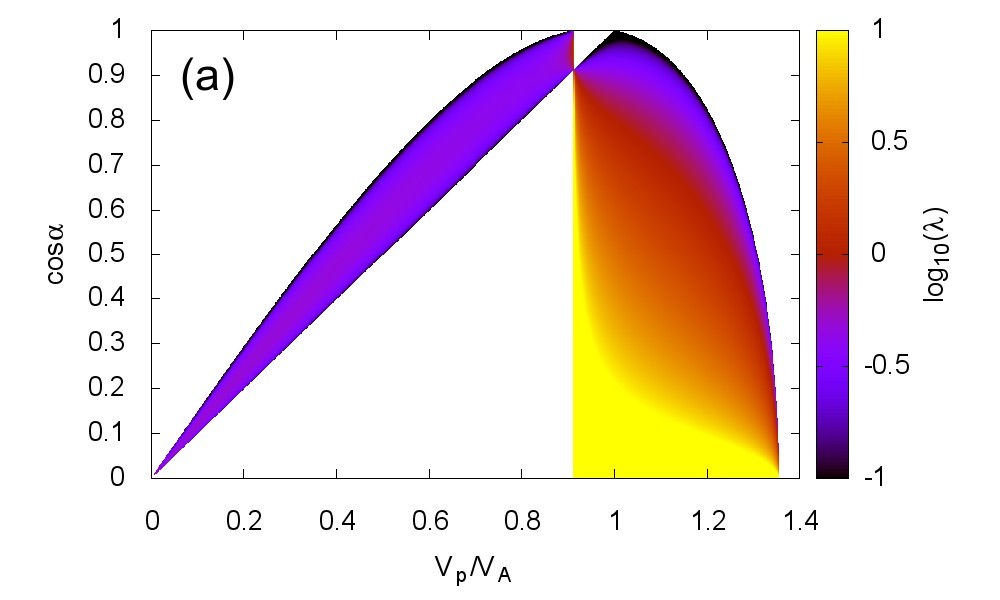

2.5 Nonlinear wave solutions of the HMHD equations as a tool for validation of numerical codes
Examples of the solitary wave solutions are shown in Fig. 2

(isotropic pressure, , , , ) and Fig. 3 (anisotropic pressure, CGL closure, , , ,

, ). Spatial profiles of all fluid variables are shown in the plots.
The solitary wave profiles can be used as the initial condition for fully time-dependent simulation. By studying wave profile distortions resulting from propagation of the waves using the numerical code one may obtain insight into properties of the numerical algorithm, its resolution scaling properties and correctness of the code implementation. For simplicity, in this approach we use polytropic state equations instead of the energy conservation equation and the magnetic diffusivity is set to zero. However, the conservation of the total energy in the absence of heat fluxes and viscous/Joule’s heating leads to polytropic relations: for the isotropic thermal pressure and the CGL relations , for the anisotropic gyrotropic pressure tensor. Therefore the polytropic relations can be used to obtain the nonlinear wave profiles that are useful for testing simulation codes with the energy conservation equation explicitly included (which is sometimes preferred to obtain better numerical stability and accuracy).
Eqs. (19) give wave profiles in the wave frame of reference, thus using them directly as the initial condition in a simulation can be considered as a steady-state testing method. In the plasma rest frame, the structures discussed above are seen as waves propagating with the velocity . Generally, by applying the velocity transformation to the solitary solutions described above it is possible to change the wave frame to another frame where the wave propagates with the velocity in the simulation box. In particular, transformation to the plasma frame is obtained for . In Sec. 5 we present some examples of the application of the nonlinear wave solutions for the validation of our numerical code for HMHD simulations.
3 Numerical scheme for time dependent simulations
In general, the set of Eqs. (12)-(15) can be considered as
| (25) |
where represents the state of the system at a given time in a spatial location , and is a nonlinear function that does not involve the time derivatives. In the proposed numerical scheme the HMHD equations are advanced in time using the second-order Runge-Kutta scheme
| (26) |
describing the time evolution from the state to , where indexes and denote two subsequent time steps, and is the integration time step.
The HMHD equations are solved on a uniform Cartesian grid. The computational domain of the size is resolved by cells, thus the spatial resolution of the grid is , , . The triplet of integers points at a cell center, numbers the cells in direction, along , and along . By using in one of the indexes in the triplet we denote a face between cells in a given direction, e.g. identifies the face between the cells and (a face normal to direction). When appears in two indexes of the triplet, we refer to the edge between cells, e.g. identifies the edge between the cells , , , . One should note that it is a standard notation used in literature (see, e.g. Refs. [18, 36], where plots illustrating the notation are presented).
All the transport equations except for Eq. (14) (magnetic field transport) are numerically solved using the Kurganov-Tadmor scheme [37] from a family of MUSCL schemes based on linear piecewise approximation for every computational cell. For those equations () from Eq. (26) is approximated as
| (27) |
As suggested by indexes containing , the fluxes are computed at the cell faces. One should also note that in the first term on the right-hand side the fluxes are computed at the faces normal to direction, in the second – normal to , in the third – normal to .
The numerical fluxes can be written as the sum , where represents the Rusanov flux for the MHD part of the equations (i.e. without the Hall term) and contains Hall corrections. The classical MHD flux is defined as
| (28) |
where the local propagation speed is the maximum absolute eigenvalue of the Jacobian of over cells . The left (L) and right (R) states are computed as
| (29) |
where and the van Leer flux limiter is used. One should note that Eqs. (29) are applied to primitive variables, that are then used to compute conservative variables and finally the fluxes. The fluxes and at the faces normal to and directions can be defined analogously to the flux at the face normal to direction by changing only the leading dimension in the above definitions.
The Hall corrections to the fluxes are computed separately using the averaged variables . To compute the current density included in the Hall velocity we need the spatial derivatives of the magnetic field components. In the scheme proposed here, the normal derivatives are computed in a different manner than the tangential derivatives. This approach is similar to that presented in Ref. [23], but we use additional averaging of the normal derivatives. The explicit form of the current density components for the faces normal to the direction is
| (30) | |||||
which can be compared with Eq. (16) in Ref. [23] to illustrate the differences. The tangential derivatives are computed by central differencing and averaging in the direction (face normal direction). In fact, the normal derivatives can be also considered as obtained by central differencing (note that the value of the derivative at is needed), but they are averaged in and directions with different weights for the central point and neighboring points . Using the current density vector we can compute the Hall corrections . The current density components (and Hall corrections) for the faces normal to the and directions can be defined analogously, according to the rules described above.
The equation of the magnetic field transport is advanced in time by using so-called flux-interpolated constrained-transport (flux-CT) approach [36], that was found to be one of the most accurate in a series of tests reported in Ref. [38]. The flux-CT approach was developed on the basis of a specific discretization scheme referred often to as a staggered-mesh transport algorithm for the magnetic field (see e.g. [39, 40]). In this approach, a discrete version of the Stokes’ theorem is used for updating magnetic field components in time. Different magnetic field components are collocated on different cell faces (normal to a given component). On the other hand, the electric field components are collocated at the edges of the cells. A version of this algorithm proposed in Ref. [36] uses a duality between the electric field and the fluxes that determine the transport of the magnetic field. Assuming that is the component of the flux normal to the direction in the equation of the transport of the component of the magnetic field, the electric field components at the cell edges are
| (31) |
The advancing of the magnetic field components in time is done by using the following scheme
| (32) |
The values of the magnetic field components in the cell centers are computed as two-point averages
| (33) |
If in the initial condition, the flux-CT scheme maintains the solenoidal magnetic field during the time evolution to the accuracy comparable with the machine round off error.
The resistive terms in Eqs. (14) and (15) also require the estimation of the current density components by differencing the magnetic field components. The same rule as in the case of the Hall-term corrections is used here, i.e. the normal derivatives use two nearest cells only, whereas the tangential derivatives are computed by central differencing and averaging in the normal direction.
The HMHD model is known to include dispersive whistler waves that impose strong constraints on the time step of the explicit numerical scheme presented above. To ensure the stability of the scheme we use , where the fastest wave speed in direction is estimated to be , is the fast magnetosonic speed [20]. In the simulations discussed below we assume the Courant number .
4 Implementation summary
The code was implemented in C/C++ in a modular manner with separate procedures for setting up problem-specific initial condition. Both periodic and floating (zero normal gradient) boundary conditions were implemented. The boundary conditions are changed at the compilation time by setting appropriate preprocessor directives during compilation. The simulation box is decomposed into smaller boxes depending on the number of available computational cores. The MPI library is used for the exchange of information between the cores about their boundaries. Simulations in one-, two- and three-dimensional simulation box are possible by setting appropriate preprocessor directives at the compilation time.
5 Numerical tests
5.1 Nonlinear solitary waves
The solitary solutions of the HMHD equations discussed in Sec. 2.3 give a possibility of verifying the correctness of the implementation and testing the accuracy of the numerical simulations. Since the amplitude of the fluctuations of the magnetic field components is not small as compared with the mean magnitude of the magnetic field (see, e.g. Figs. 2 and 3), this testing method can be considered as a validation in the nonlinear regime. The exact analytical form for HMHD solitary solutions is not known in general, but solitary waves can be obtained as a numerical solution of the set of ordinary differential equations (19). In its own frame of reference a solitary wave is a steady-state solution. We can easily change it into a propagating solution by simply adding a constant to velocity component of the solitary wave profile. By rotating the structure (and all vector quantities) in a two- or three-dimensional simulation box we can test oblique propagation with respect to the grid. In tests presented in this subsection the magnetic diffusivity is .
One should note that using solitary
solutions for testing the time-dependent simulations imposes strong
requirements on the accuracy of the solitary solution itself. In the
discussion presented below we used a procedure odeint() from
Ref. [41] with an accuracy parameter for solving
Eq. (19) and a procedure rtbis() with a parameter
for Eqs. (16) or (17). In the testing procedure reported below,
one solution with 16384 points is obtained by integration of ODE and then it
is used as the initial condition in simulations with the resolution
by removing every points. It is also used as a base
solution for oblique propagation with respect to the grid in 2D simulations as discussed below.
The first test verifies the scheme properties for a steady-state solution. Solitary waves shown in Figs. 2 (isotropic pressure) and 3 (anisotropic pressure) are used as the initial


condition. The simulation is done in the frame of the wave, thus we can check the accuracy of the code for maintaining a steady-state solution in the one-dimensional simulation. Periodic boundary conditions are used. For the isotropic case the size of the simulation domain is , for the anisotropic case . Six resolutions are tested: 128, 256, 512, 1024, 2048, 4096 grid points, the final simulation time is for the isotropic case and for the anisotropic case. Fig. 4 shows the time dependence of the error of the transversal component of the magnetic field that increases with time as indicating nearly diffusive character of errors introduced by the numerical code. Resolution change of factor 2 gives 4-fold smaller error that confirms the expected second-order scaling of the numerical scheme under verification.
In the second test, the same solitary solution is amended by adding a constant propagation velocity (it corresponds to the propagation in the simulation box frame with the Alfven speed), which makes it possible to test the code for a propagating structure. Periodic boundary conditions are applied and for the anisotropic pressure case shown in Fig. 3, the size of the simulation domain is . Therefore after the time the wave should arrive back at its initial position. Fig. 5(a) shows dependence

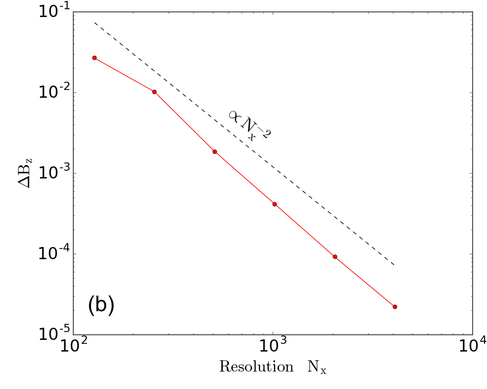
of for this type of test for six different resolutions. Since the amplitude and velocity of solitary waves are related, the amplitude decrease related to errors introduced by the numerical scheme changes the propagation speed of the wave with respect to plasma frame. This is clearly seen for low resolutions as a shift between the time of the local minimum of and . As the resolution increases the shift becomes smaller. In Fig. 5(b) we show the minimum of from Fig. 5(a) as a function of the resolution , which confirms clearly the second-order scaling of the numerical errors . Fig. 5 shows results for the anisotropic-pressure case, a similar study for the isotropic pressure gives the same scaling of numerical errors (not shown here).
Fig. 6 summarizes results of testing of oblique propagation


of a solitary wave in 2D simulation box for different angles between the wave normal direction and direction. The wave propagates in the simulation box with the velocity , similarly to 1D propagation test, the size of the simulation domain is . Results for three resolutions are shown: , , for the anisotropic-pressure solitary wave shown in Fig. 3. Periodic boundary conditions are applied in and directions. Fig. 6 suggests a weak dependence of the errors introduced by the numerical scheme on the propagation angle with respect to the computational grid. As illustrated in Fig. 7 numerical errors mainly contribute to a decrease of the wave amplitude, which can be seen by comparison of the range in the color bars in panels (a),(c),(e) with respect to (b),(d),(f). The numerical errors also introduce asymmetry of the leading edge with respect to the trailing edge (the wave propagates to the right, thus leading edge is on the right and trailing edge on the left), which is particularly well seen by comparison of panels (a) and (b). Similar results have been obtained for the isotropic case (not shown here).
Another test is intended to check the behavior of the code in the case of strongly nonlinear localized interactions. The simulation domain is 3D, the grid resolution is , the size is , periodic boundary conditions are used in all directions. In the initial condition the solitary wave from Fig. 2 (isotropic pressure) is set up in the middle of the box (blue planar structure in Fig. 8(a)).


Additionally a localized spherically-symmetric density enhancement (blob) is set up (the center of the blob is initially located at , ). The simulation is done in the soliton frame, thus the blob (that can be considered as an entropy wave perturbation) is advected by the flow towards the planar soliton. Fig. 8(b) shows a moment of the interaction of the blob and the solitary wave, when the structures are being distorted by the interaction process. During the interaction, the blob is constantly blown downward (towards ) by the flow inside the solitary wave ( in the solitary wave as seen in Fig. 2). After having pierced the solitary wave, the blob is advected by the flow towards the boundary as seen in Fig. 8(c). The interaction process produces a perturbation in the planar soliton that is advected downward by the flow inside the solitary wave. The perturbation is seen at the bottom and at the top of the simulation box in Fig. 8(c) due to periodic boundary conditions applied in the direction.
5.2 Magnetic reconnection
HMHD codes are conventionally tested with a well-studied (also by MHD and kinetic codes) problem, the Geospace Environmental Modeling (GEM) magnetic reconnection challenge [2]. The exact form of the solution is not known in this case, but solutions obtained using our code can be compared with a number of solutions published elsewhere. One should note that the problem of magnetic reconnection is quite specific as it involves dynamics in regions, where particles are weakly magnetized or unmagnetized. For these “diffusive” regions the isotropic and gyrotropic models presented in our paper are not good approximations since non-gyrotropic pressure tensor should be considered to describe properly the underlying physics [33]. Even though HMHD description gives a simplified picture, by including the Hall term we can obtain reconnection rate much larger that in resistive MHD and in some cases comparable with kinetic description. This kind of approach can be useful for some problems of interest, where one considers consequences of fast magnetic reconnection on large-scale dynamics, rather than details of the diffusion-region physics. In any case, the GEM reconnection challenge has become a standard benchmark showing the correctness of implementation and reliability of the applied numerical approach, therefore we present below tests for this problem.
In our simulation the problem is formulated in – plane. The initial condition is
| (34) |
where , , , , , . The simulation domain size is , . The spatial resolution is points. In the direction periodic boundary conditions are applied, in the direction we use zero-gradient floating boundary. For reference purposes, apart from the HMHD computations, we computed also a solution within classical MHD framework (without the Hall corrections). A constant magnetic diffusivity was used in the HMHD and MHD simulations with the isotropic pressure model including the total energy conservation equation.
Fig. 9 shows the distributions of the out-of-plane component of the current density vector


for for the HMHD and MHD models. The distributions of the current density are very similar to those presented in Ref. [43], in particular for the HMHD case [Fig. 9(a)] the current density is concentrated in the center of the simulation box. Some papers (see, e.g. Ref. [23]) reported an island in the center of the simulation box in the HMHD case, this type of behavior appears in our simulations but for smaller values of the magnetic diffusivity (not shown here). Reconnection along elongated current sheet for the MHD case [Fig. 9(b)] is consistent with the Sweet-Parker model predictions. At the left- and right-hand side of the simulation box in Fig. 9 one can see some gradients that are related to periodic boundary conditions and can be seen in other simulations of the magnetic reconnection sites (see e.g. [44]).
The time evolution of the reconnected flux is shown in Fig. 10. The HMHD flux is several times larger than the MHD flux, as typically obtained in this type of simulations [2, 20, 23]. One should note that the time dependence of the reconnected flux is quantitatively very similar to results presented in Ref. [2] for both the HMHD and the MHD cases.

5.3 Firehose instability
Pressure anisotropy may provide free energy for the growth of instabilities in plasmas. One of the examples is the firehose instability growing when [18, 34, 45, 46]. We present results for 2D simulation box, where the domain size is and for 3D simulations where . The mean magnetic field is set up along the axis. Periodic boundary conditions are applied in all directions. In the initial condition low-amplitude and fluctuations with randomized phases are set up, the fluctuations are not correlated initially. In tests presented in this subsection the magnetic diffusivity is .
Fig. 11 shows the growth of the amplitude of fluctuations from the initial noise


for and (in the initial condition) for 2D and 3D simulations. The square of the amplitude grows exponentially approx. 17 orders of magnitude until is reached, where . One should note that the saturation level is consistent with the predictions of the quasilinear theory [17] and similar to the saturation amplitude obtained in 2D high- kinetic simulation results reported in Ref. [47].
Fig. 12(a) shows that during the growth of the fluctuations the average pressure anisotropy level drops just below the


threshold for the firehose instability. Fig. 12(b) shows results of testing the dependence of the growth rate on the initial pressure anisotropy for constant in 2D simulations. A power-law relationship is obtained with .
As illustrated in Fig. 13 (for 2D) and Fig. 14 (for 3D) the fastest growing mode is oblique with respect to the mean magnetic field (oriented along the axis).


Initially locally regular distribution of (shown in Figs. 13(a) and 14(a) for ) gradually changes in time towards a more turbulent state (shown in Figs. 13(b) and 14(b) for ). The magnetic field lines can be seen to be weakly perturbed in the simulation plane in 2D case, because fluctuations of the (out-of-plane) component grow preferentially in this case as seen in Fig. 11. The perturbation of the magnetic field lines in the 3D case is visualized in Fig. 15. The behavior of the firehose fluctuations is generally similar to results of 2D high- kinetic simulations reported in Ref. [18]. To our knowledge, we present in our paper the first results of three-dimensional structure of the firehose instability fluctuations.


One should note that fluid models give the same threshold for the parallel firehose instability as the kinetic models, but a more stringent threshold is obtained within kinetic theory for the oblique firehose instability [12, 48, 49]. This leads typically to preferential growth of the oblique mode, when the parallel and the oblique instabilities compete. In our simulations within the HMHD framework, the oblique mode grows in the system, which is similar to kinetic models and suggests that the HMHD model may capture some elements of the oblique-parallel firehose mode competition. Systematic analysis of the dispersion relation would be interesting in this context. To our knowledge, only the parallel mode of the firehose instability in HMHD has been systematically investigated [34].
6 Summary
We present a second-order accurate solver for the HMHD equations with anisotropic or isotropic thermal pressure. Both explicit energy conservation equation and polytropic state equations can be used in this approach as the closure for the HMHD model. The implemented code was validated using test problems previously described in the literature: the magnetic reconnection process and the growth of the firehose instability. Additionally, we propose a new validation method for the HMHD codes based on solitary waves that provides a possibility of quantitative testing in nonlinear regime as a complementary approach to standard tests using small-amplitude whistler waves. Quantitative tests of the accuracy and the performance of the implemented code show the fidelity of the proposed approach. It is demonstrated that the efficiency of the proposed approach and its implementation are sufficient for three-dimensional simulations within the HMHD framework.
The present formulation of the numerical scheme for the HMHD equations is purely explicit and can be accelerated by using, e.g. a subcycling procedure for the integration of the equation for the magnetic field transport as proposed in Ref. [20]. Another possibility of acceleration of the computations includes applying an implicit scheme, where stability of the code is not constrained by the CFL condition for whistler waves at the expense of the accuracy of the computations. In these contexts the proposed method of validation based on solitary waves can be particularly useful for testing the accuracy of the modified approaches. Since in some aspects the HMHD model can be considered as a low-beta approximation for kinetic models, the testing method based on solitary waves presented in this paper has also conceivable applications for testing/validation of kinetic (particle-in-cell or Vlasov-Maxwell) models.
Acknowledgments
This work has been supported by the Polish National Science Centre (DEC-2012/05/B/ST9/03916). One of the authors (M.S.) of this project has received funding from the European Union’s Horizon 2020 research and innovation programme under the Marie Sklodowska-Curie grant agreement No 657251 (ASTROMULTISCALE). The discussion presented in the paper reflects only the authors’ view and the European Commission is not responsible for any use that may be made of the information it contains. M.S. wishes to acknowledge support from the International Space Science Institute for the team “Facing the Most Pressing Challenges to Our Understanding of the Heliosheath and its Outer Boundaries”.
References
References
- [1] J. D. Huba, Hall magnetohydrodynamics in space and laboratory plasmas, Phys. Plasmas 2 (1995) 2504–2513. doi:10.1063/1.871212.
- [2] J. Birn, J. F. Drake, M. A. Shay, B. N. Rogers, R. E. Denton, M. Hesse, M. Kuznetsova, Z. W. Ma, A. Bhattacharjee, A. Otto, P. L. Pritchett, Geospace Environmental Modeling (GEM) magnetic reconnection challenge, J. Geophys. Res. 106 (2001) 3715–3720. doi:10.1029/1999JA900449.
- [3] Z. W. Ma, A. Bhattacharjee, Hall magnetohydrodynamic reconnection: The Geospace Environment Modeling challenge, J. Geophys. Res. 106 (2001) 3773–3782. doi:10.1029/1999JA001004.
- [4] J. D. Huba, L. I. Rudakov, Hall Magnetic Reconnection Rate, Phys. Rev. Lett. 93 (17) (2004) 175003. doi:10.1103/PhysRevLett.93.175003.
- [5] K. Stasiewicz, Reinterpretation of mirror modes as trains of slow magnetosonic solitons, Geophys. Res. Lett. 31 (2004) 21804. doi:10.1029/2004GL021282.
- [6] K. Stasiewicz, Theory and Observations of Slow-Mode Solitons in Space Plasmas, Phys. Rev. Lett. 93 (12) (2004) 125004. doi:10.1103/PhysRevLett.93.125004.
- [7] K. Stasiewicz, Nonlinear Alfvén, magnetosonic, sound, and electron inertial waves in fluid formalism, J. Geophys. Res. 110 (2005) 3220. doi:10.1029/2004JA010852.
- [8] M. Strumik, K. Stasiewicz, C. Z. Cheng, B. Thidé, Evolution of large-scale magnetosonic structures to trains of solitary waves, J. Geophys. Res. 116 (2011) 7209. doi:10.1029/2011JA016565.
- [9] P. D. Mininni, D. O. Gómez, S. M. Mahajan, Direct Simulations of Helical Hall-MHD Turbulence and Dynamo Action, Astrophys. J. 619 (2005) 1019–1027. doi:10.1086/426534.
- [10] P. Dmitruk, W. H. Matthaeus, Test particle acceleration in three-dimensional Hall MHD turbulence, J. Geophys. Res. 111 (10) (2006) 12110. doi:10.1029/2006JA011988.
- [11] J. C. Kasper, A. J. Lazarus, S. P. Gary, Wind/SWE observations of firehose constraint on solar wind proton temperature anisotropy, Geophys. Res. Lett. 29 (2002) 1839. doi:10.1029/2002GL015128.
- [12] P. Hellinger, P. Trávníček, J. C. Kasper, A. J. Lazarus, Solar wind proton temperature anisotropy: Linear theory and WIND/SWE observations, Geophys. Res. Lett. 33 (2006) 9101. doi:10.1029/2006GL025925.
- [13] L. Matteini, S. Landi, P. Hellinger, F. Pantellini, M. Maksimovic, M. Velli, B. E. Goldstein, E. Marsch, Evolution of the solar wind proton temperature anisotropy from 0.3 to 2.5 AU, Geophys. Res. Lett. 34 (2007) 20105. doi:10.1029/2007GL030920.
- [14] S. D. Bale, J. C. Kasper, G. G. Howes, E. Quataert, C. Salem, D. Sundkvist, Magnetic Fluctuation Power Near Proton Temperature Anisotropy Instability Thresholds in the Solar Wind, Phys. Rev. Lett. 103 (21) (2009) 211101. doi:10.1103/PhysRevLett.103.211101.
- [15] A. A. Schekochihin, S. C. Cowley, R. M. Kulsrud, G. W. Hammett, P. Sharma, Plasma Instabilities and Magnetic Field Growth in Clusters of Galaxies, Astrophys. J. 629 (2005) 139–142. doi:10.1086/431202.
- [16] P. Hellinger, P. M. Trávníček, Oblique proton fire hose instability in the expanding solar wind: Hybrid simulations, J. Geophys. Res. 113 (A12) (2008) 10109. doi:10.1029/2008JA013416.
- [17] A. A. Schekochihin, S. C. Cowley, R. M. Kulsrud, M. S. Rosin, T. Heinemann, Nonlinear Growth of Firehose and Mirror Fluctuations in Astrophysical Plasmas, Phys. Rev. Lett. 100 (8) (2008) 081301. doi:10.1103/PhysRevLett.100.081301.
- [18] M. W. Kunz, A. A. Schekochihin, J. M. Stone, Firehose and Mirror Instabilities in a Collisionless Shearing Plasma, Phys. Rev. Lett. 112 (20) (2014) 205003. doi:10.1103/PhysRevLett.112.205003.
- [19] S. Servidio, K. T. Osman, F. Valentini, D. Perrone, F. Califano, S. Chapman, W. H. Matthaeus, P. Veltri, Proton Kinetic Effects in Vlasov and Solar Wind Turbulence, Astrophys. J. Lett. 781 (2014) L27. doi:10.1088/2041-8205/781/2/L27.
- [20] J. D. Huba, Hall Magnetohydrodynamics - A Tutorial, in: J. Büchner, C. Dum, M. Scholer (Eds.), Space Plasma Simulation, Vol. 615 of Lecture Notes in Physics, Berlin Springer Verlag, 2003, pp. 166–192.
- [21] L. Chacón, D. A. Knoll, A 2D high-/ Hall MHD implicit nonlinear solver, J. Comp. Phys. 188 (2003) 573–592. doi:10.1016/S0021-9991(03)00193-1.
- [22] D. Laveder, D. Borgogno, T. Passot, P. L. Sulem, On a semi-implicit scheme for spectral simulations of dispersive magnetohydrodynamics, Computer Physics Communications 180 (2009) 1860–1869. doi:10.1016/j.cpc.2009.05.018.
- [23] G. Tóth, Y. Ma, T. I. Gombosi, Hall magnetohydrodynamics on block-adaptive grids, Journal of Computational Physics 227 (2008) 6967–6984. doi:10.1016/j.jcp.2008.04.010.
- [24] N. A. Krall, A. W. Trivelpiece, Principles of plasma physics, McGraw-Hill, 1973.
- [25] A. Le, J. Egedal, W. Daughton, W. Fox, N. Katz, Equations of State for Collisionless Guide-Field Reconnection, Phys. Rev. Lett. 102 (8) (2009) 085001. doi:10.1103/PhysRevLett.102.085001.
- [26] J. Egedal, A. Le, W. Daughton, A review of pressure anisotropy caused by electron trapping in collisionless plasma, and its implications for magnetic reconnection, Phys. Plasmas 20 (6) (2013) 061201. doi:10.1063/1.4811092.
- [27] J. A. Bittencourt, Fundamentals of Plasma Physics, Springer-Verlag, 2004.
- [28] L.-N. Hau, T.-D. Phan, B. U. O. Sonnerup, G. Paschmann, Double-polytropic closure in the magentosheath, Geophys. Res. Lett. 20 (1993) 2255–2258. doi:10.1029/93GL02491.
- [29] G. F. Chew, M. L. Goldberger, F. E. Low, The Boltzmann Equation and the One-Fluid Hydromagnetic Equations in the Absence of Particle Collisions, Royal Society of London Proceedings Series A 236 (1956) 112–118. doi:10.1098/rspa.1956.0116.
- [30] A. Hakim, J. Loverich, U. Shumlak, A high resolution wave propagation scheme for ideal Two-Fluid plasma equations, J. Comp. Phys. 219 (2006) 418–442. doi:10.1016/j.jcp.2006.03.036.
- [31] D. S. Balsara, T. Amano, S. Garain, J. Kim, A high-order relativistic two-fluid electrodynamic scheme with consistent reconstruction of electromagnetic fields and a multidimensional Riemann solver for electromagnetism, J. Comp. Phys. 318 (2016) 169–200. doi:10.1016/j.jcp.2016.05.006.
- [32] T. Amano, A second-order divergence-constrained multidimensional numerical scheme for relativistic two-fluid electrodynamics, Astrophys. J.In press "arXiv:1607.08487".
- [33] L. Wang, A. H. Hakim, A. Bhattacharjee, K. Germaschewski, Comparison of multi-fluid moment models with particle-in-cell simulations of collisionless magnetic reconnection, Phys. Plasmas 22 (1) (2015) 012108. doi:10.1063/1.4906063.
- [34] B.-J. Wang, L.-N. Hau, Parallel proton fire hose instability in gyrotropic Hall MHD model, J. Geophys. Res. 115 (2010) 4105. doi:10.1029/2009JA014947.
- [35] J. F. McKenzie, E. Dubinin, K. Sauer, T. B. Doyle, The application of the constants of motion to nonlinear stationary waves in complex plasmas: a unified fluid dynamic viewpoint, J. Plasma Phys. 70 (2004) 431–462. doi:10.1017/S0022377803002654.
- [36] D. S. Balsara, D. S. Spicer, A Staggered Mesh Algorithm Using High Order Godunov Fluxes to Ensure Solenoidal Magnetic Fields in Magnetohydrodynamic Simulations, J. Comp. Phys. 149 (1999) 270–292. doi:10.1006/jcph.1998.6153.
- [37] A. Kurganov, E. Tadmor, New High-Resolution Central Schemes for Nonlinear Conservation Laws and Convection-Diffusion Equations, J. Comp. Phys. 160 (2000) 241–282. doi:10.1006/jcph.2000.6459.
- [38] G. Tóth, The Constraint in Shock-Capturing Magnetohydrodynamics Codes, J. Comp. Phys. 161 (2000) 605–652. doi:10.1006/jcph.2000.6519.
- [39] K. Yee, Numerical solution of inital boundary value problems involving maxwell’s equations in isotropic media, IEEE Transactions on Antennas and Propagation 14 (1966) 302–307. doi:10.1109/TAP.1966.1138693.
- [40] C. R. Evans, J. F. Hawley, Simulation of magnetohydrodynamic flows - A constrained transport method, Astrophys. J. 332 (1988) 659–677. doi:10.1086/166684.
- [41] W. H. Press, S. A. Teukolsky, W. T. Vetterling, B. P. Flannery, Numerical recipes in C. The art of scientific computing, Cambridge: University Press, 1992, 1992.
- [42] P. Ramachandran, G. Varoquaux, Mayavi: 3d visualization of scientific data, Computing in Science & Engineering 13 (2) (2011) 40–51. doi:10.1109/MCSE.2011.35.
- [43] J. Birn, M. Hesse, Geospace Environment Modeling (GEM) magnetic reconnection challenge: Resistive tearing, anisotropic pressure and hall effects, J. Geophys. Res. 106 (2001) 3737–3750. doi:10.1029/1999JA001001.
- [44] P. A. Cassak, M. A. Shay, J. F. Drake, Catastrophe Model for Fast Magnetic Reconnection Onset, Phys. Rev. Lett. 95 (23) (2005) 235002. doi:10.1103/PhysRevLett.95.235002.
- [45] C. F. Kennel, R. Z. Sagdeev, Collisionless shock waves in high plasmas: 1, J. Geophys. Res. 72 (1967) 3303–3326. doi:10.1029/JZ072i013p03303.
- [46] B. J. Wang, L. N. Hau, MHD aspects of fire-hose type instabilities, J. Geophys. Res. 108 (2003) 1463. doi:10.1029/2003JA009986.
- [47] M. W. Kunz, J. M. Stone, X.-N. Bai, Pegasus: A new hybrid-kinetic particle-in-cell code for astrophysical plasma dynamics, J. Comp. Phys. 259 (2014) 154–174. doi:10.1016/j.jcp.2013.11.035.
- [48] P. Hellinger, H. Matsumoto, New kinetic instability: Oblique Alfvén fire hose, J. Geophys. Res. 105 (2000) 10519–10526. doi:10.1029/1999JA000297.
- [49] P. Hellinger, H. Matsumoto, Nonlinear competition between the whistler and Alfvén fire hoses, J. Geophys. Res. 106 (2001) 13215–13218. doi:10.1029/2001JA900026.