跳到论文正文
W Papers独立论文阅读器 arXiv:1610.09109 论文正文 计算阅读时间 · 0%
引用这篇论文根据当前论文元数据生成,正式投稿前建议核对。


License: arXiv.org perpetual non-exclusive license
arXiv:1610.09109v3 [math.ST] 17 Jan 2018

Improved Classification Rates under Refined Margin Conditions

Ingrid Blaschzyk    Ingo Steinwart
Abstract

In this paper we present a simple partitioning based technique to refine the statistical analysis of classification algorithms. The core of our idea is to divide the input space into two parts such that the first part contains a suitable vicinity around the decision boundary, while the second part is sufficiently far away from the decision boundary. Using a set of margin conditions we are then able to control the classification error on both parts separately. By balancing out these two error terms we obtain a refined error analysis in a final step. We apply this general idea to the histogram rule and show that even for this simple method we obtain, under certain assumptions, better rates than the ones known for support vector machines, for certain plug-in classifiers, and for a recently analyzed tree based adaptive-partitioning ansatz. Moreover, we show that a margin condition which sets the critical noise in relation to the decision boundary makes it possible to improve the optimal rates proven for distributions without this margin condition.

and

Institute for Stochastics and Applications
University of Stuttgart
Pfaffenwaldring 57
D-70569 Stuttgart
??

Contents

1 Introduction

Given a dataset D:=((x1,y1),…,(xn,yn))D:=((x_{1},y_{1}),\ldots,(x_{n},y_{n})) of observations drawn in an i.i.d. fashion from a probability measure PP on X×YX\times Y, where X⊂ℝdX\subset\mathbb{R}^{d} and Y:={−1,1}Y:=\{-1,1\}, the learning goal of binary classification is to find a decision function fD:X→{−1,1}f_{D}\colon X\to\{{-1,1\}} such that for new data (x,y)(x,y) we have fD​(x)=yf_{D}(x)=y with high probability.

The problem of classification is, apart from regression, one of the most considered problems in learning theory and many classical learning methods have been presented in the literature such as histogram rules, nearest neighbor methods or moving window rules. A general reference for these methods is [4]. Several more recent methods use trees to build a classifier, for example the random forest algorithm, introduced in [3], makes a prediction by a majority vote over a collection of random forest trees. Another example is the tree based adaptive-partitioning algorithm, presented in [2]. Here, a classifier is picked by empirical risk minimization over a nested sequence (Sm)m≥1(S_{m})_{m\geq 1} of families of sets which is based on dyadic or decorated tree partitions. Examples of non-tree based algorithms are described in [1] and [7]. There, the final classifier is found by empirical risk minimization over a suitable grid of plug-in rules or is derived by plug-in kernel, partitioning or nearest neighbor classification rules. Another non-tree based algorithm is, for example, the support vector machine (SVM), which solves a regularized empirical risk minimization problem over a reproducing kernel Hilbert space HH. For more details on statistical properties of SVM for classification we refer the reader to [10, Chapter 8].

In this paper we discuss a partitioning based technique to analyse the statistical properties of classification algorithms. In particular we show for the histogram rule that under certain assumptions this technique leads to rates, which are faster than the rates obtained in [1, 2, 7], and [10]. To be more precise, we divide the input space XX into two overlapping regions that are adjustable by a parameter rr in such a way that one set, which we will denote by NrN_{r}, contains points near the decision boundary, whereas the other set FrF_{r} contains those that are sufficiently far away from the decision boundary. We examine the excess risks over these two sets separately by applying an oracle inequality for empirical risk minimizers on both parts. It turns out that we have no approximation error on FrF_{r} and that we obtain, under a suitable assumption which relates critical noise to the decision boundary, an optimal variance bound on FrF_{r}, which in turn leads to an 𝒪⁡(n−1)\mathcal{O}(n^{-1}) behavior of the excess risk on FrF_{r}. However, this bound still depends on the parameter rr, namely it increases for r→0r\rightarrow 0. In contrast, our bound on the risk on NrN_{r} decreases for r→0r\rightarrow 0. By balancing out these two risks with respect to rr we obtain a refined bound on XX under additional assumptions describing the concentration of mass around the decision boundary.

A more detailed discussion on this technique and the statistical results, which include rate adaptivity, are presented in Section 3. Moreover, a comparison of the resulting learning rates to the ones known for the SVM, for certain plug-in classification rules and the tree based adaptive-partitioning algorithm described in [2] can be found at the end of Section 4. In particular, we show that the above mentioned assumption that relates the location of critical noise to the decision boundary has an essential influence on our learning rates such that we outperform under a common set of assumptions the optimal rates obtained for the classifier in [1]. Furthermore, we show that if we omit the latter assumption, we obtain exactly the optimal rate of [1]. We note that all proofs are deferred to Section 5.

2 General Assumptions

To describe our learning goal we consider in the following the classification loss L:=Lclass:Y×ℝ→[0,∞)L:={{L}_{\mathrm{class}}}:Y\times\mathbb{R}\to[0,\infty), defined by L(y,t):=𝟏(−∞,0](y⋅signt)L(y,t):=\boldsymbol{1}_{(-\infty,0]}(y\cdot\text{sign}t) for y∈Y,t∈ℝy\in Y,t\in\mathbb{R}, where 𝟏(−∞,0]\boldsymbol{1}_{(-\infty,0]} denotes the indicator function on (−∞,0](-\infty,0]. We define the risk of a measurable estimator f:X→ℝf:X\to\mathbb{R} by

ℛL,P​(f):=∫X×YL⁡(y,f⁡(x))​𝑑P​(x,y)\displaystyle{{\cal R}_{L,P}(f)}:=\int_{X\times Y}L(y,f(x))\,dP(x,y)

and the empirical risk by

ℛL,D​(f):=1n​∑i=1nL⁡(yi,f⁡(xi)),\displaystyle{{\cal R}_{L,D}(f)}:=\frac{1}{n}\sum_{i=1}^{n}L(y_{i},f(x_{i})),

where D:=1n​∑i=1nδ(xi,yi)D:=\frac{1}{n}\sum_{i=1}^{n}\delta_{(x_{i},y_{i})} denotes the average of Dirac measures δ(xi,yi)\delta_{(x_{i},y_{i})} at (xi,yi)(x_{i},y_{i}). The smallest possible risk

ℛL,P∗:=inff:X→ℝℛL,P(f)\displaystyle{{\cal R}_{L,P}^{*}}:=\inf_{f\colon X\to\mathbb{R}}{{\cal R}_{L,P}(f)}

is called the Bayes risk, and a measurable function fL,P∗:X→ℝf^{\ast}_{L,P}\colon X\to\mathbb{R} so that ℛL,P​(fL,P∗)=ℛL,P∗{{\cal R}_{L,P}(f^{\ast}_{L,P})}={{\cal R}_{L,P}^{*}} holds is called Bayes decision function. Recall that the Bayes decision function fL,P∗f^{\ast}_{L,P} for the classification loss is given by sign​(2​P​(y=1|x)−1)\text{sign}(2P(y=1|x)-1) for x∈Xx\in X, where P(⋅|x)P(\,\cdot\,|x) is a regular conditional probability on YY given xx.
Let us now briefly describe a particular histogram rule. To this end, let 𝒜=(Aj)j≥1\mathcal{A}=(A_{j})_{j\geq 1} be a partition of ℝd\mathbb{R}^{d} into cubes of side length s∈(0,1]s\in(0,1] and X:=[−1,1]dX:=\left[-1,1\right]^{d}. For x∈Xx\in X we denote by A⁡(x)A(x) the unique cell of 𝒜\mathcal{A} with x∈A⁡(x)x\in A(x) and call the map hP,s:X→Yh_{P,s}\colon X\to Y defined by

hP,s​(x):={−1if​fP,s​(x)<0,1if​fP,s​(x)≥0,\displaystyle h_{P,s}(x):=\begin{cases}-1&\text{if}\,f_{P,s}(x)<0,\\ 1&\text{if}\,f_{P,s}(x)\geq 0,\end{cases} (1)

where fP,s​(x):=P⁡(A⁡(x)×{1})−P⁡(A⁡(x)×{−1})f_{P,s}(x):=P(A(x)\times\{1\})-P(A(x)\times\{-1\}), infinite sample histogram rule. For a dataset DD we further write

fD,s(x):=1n∑i=1n𝟏{yi=+1}𝟏A⁡(x)(xi)−1n∑i=1n𝟏{yi=−1}𝟏A⁡(x)(xi).\displaystyle f_{D,s}(x):=\frac{1}{n}\sum_{i=1}^{n}\boldsymbol{1}_{\{y_{i}=+1\}}\boldsymbol{1}_{A(x)}(x_{i})-\frac{1}{n}\sum_{i=1}^{n}\boldsymbol{1}_{\{y_{i}=-1\}}\boldsymbol{1}_{A(x)}(x_{i}).

Thus, the empirical histogram is defined by hD,s:=sign​fD,sh_{D,s}:=\text{sign}f_{D,s}. We define the set ℱ\mathcal{F} by

ℱ:={∑Aj∩[−1,1]d≠∅cj​𝟏Aj:cj∈{−1,1}}.\displaystyle\mathcal{F}:=\left\{\,\sum_{A_{j}\cap\left[-1,1\right]^{d}\neq\emptyset}c_{j}\boldsymbol{1}_{A_{j}}\colon c_{j}\in\{-1,1\}\,\right\}.

Then, it is easy to show that the empirical histogram rule hD,sh_{D,s} is an empirical risk minimizer over ℱ\mathcal{F} for the classification loss, that means

ℛL,D​(hD,s)=inff∈ℱℛL,D​(f).\displaystyle{{\cal R}_{L,D}(h_{D,s})}=\inf_{f\in\mathcal{F}}{{\cal R}_{L,D}(f)}.

Since we aim in a further step to examine the risk on subsets of XX consisting of cells, we have to specify the loss on those subsets. Therefore, we define for an arbitrary index set J⊂{ 1,…,m}J\subset\{\,1,\ldots,m\,\} the set

TJ:=⋃j∈JAj\displaystyle T_{J}:=\bigcup_{j\in J}A_{j} (2)

and the related loss LTJ:X×Y×ℝ→[0,∞)L_{T_{J}}:X\times Y\times\mathbb{R}\rightarrow[0,\infty) by

LTJ​(x,y,t):=𝟏⋃j∈JAj​(x)​Lclass​(y,t).\displaystyle L_{T_{J}}(x,y,t):=\boldsymbol{1}_{\bigcup_{j\in J}A_{j}}(x){{L}_{\mathrm{class}}}(y,t). (3)

Furthermore, we define the risk over TJT_{J} by

ℛLTJ,P​(f):=∫X×YLTJ​(x,y,f⁡(x))​𝑑P​(x,y)\displaystyle{{\cal R}_{L_{T_{J}},P}(f)}:=\int_{X\times Y}L_{T_{J}}(x,y,f(x))\,dP(x,y)

and define the shortcut LTJ∘f:=LTJ​(x,y,f⁡(x))L_{T_{J}}\circ f:=L_{T_{J}}(x,y,f(x)).

We denote by PnP^{n} the product measure of the probability measure PP. As mentioned in the introduction, we have to make assumptions on PP to obtain rates. Therefore, we recall some notions from [10, Chapter 8] which describe the behavior of PP in the vicinity of the decision boundary. To this end, let η:X→[0,1]\eta\colon X\to[0,1], defined by η⁡(x):=P⁡(y=1|x)\eta(x):=P(y=1|x) for x∈Xx\in X, be a version of the posterior probability of PP, that is, that the probability measures P(⋅|x)P(\,\cdot\,|x) form a regular conditional probability of P. Clearly, if we have η⁡(x)=0\eta(x)=0 resp. η⁡(x)=1\eta(x)=1 for x∈Xx\in X we observe the label y=−1y=-1 resp. y=1y=1 with probability 11. Otherwise, if, e.g., η⁡(x)∈[1/2,1)\eta(x)\in[1/2,1) we observe the label y=−1y=-1 with the probability 1−η⁡(x)∈(0,1/2]1-\eta(x)\in(0,1/2] and we call the latter probability noise. Obviously, in the worst case this probability equals 1/21/2 and we define the set containing those x∈Xx\in X by X0:={x∈X:η⁡(x)=1/2}X_{0}:=\{\,x\in X\colon\eta(x)=1/2\,\}. Furthermore, we write

X1\displaystyle X_{1} :={x∈X:η⁡(x)>1/2},\displaystyle:=\{\,x\in X\colon\eta(x)>1/2\,\},
X−1\displaystyle X_{-1} :={x∈X:η⁡(x)<1/2}.\displaystyle:=\{\,x\in X\colon\eta(x)<1/2\,\}.

Then, the function Δη:X→[0,∞]\Delta_{\eta}\colon X\to[0,\infty] defined by

Δη​(x):={d⁡(x,X1)if​x∈X−1,d⁡(x,X−1)if​x∈X1,0otherwise,\displaystyle\begin{split}\Delta_{\eta}(x):=\begin{cases}d(x,X_{1})&\text{if}\,x\in X_{-1},\\ d(x,X_{-1})&\text{if}\,x\in X_{1},\\ 0&\text{otherwise},\end{cases}\end{split} (4)

where d⁡(x,A):=infx′∈Ad⁡(x,x′)d(x,A):=\inf_{x^{\prime}\in A}d(x,x^{\prime}), is called distance to the decision boundary. This helps us to describe the mass of the marginal distribution PXP_{X} of PP around the decision boundary by the following exponents. We say that PP has margin exponent (ME) α∈(0,∞]\alpha\in(0,\infty] if there exists a constant cME>0c_{\text{ME}}>0 such that

PX({Δη(x)<t})≤(cMEt)α\displaystyle P_{X}(\{\Delta_{\eta}(x)<t\})\leq(c_{\text{ME}}t)^{\alpha}

for all t>0t>0. Descriptively, the ME α\alpha measures the amount of mass close to the decision boundary. Therefore, large values of α\alpha are better since they reflect a low concentration of mass in this region, which makes the classification easier. Furthermore, we say that PP has margin-noise exponent (MNE) β∈(0,∞]\beta\in(0,\infty] if there exists a constant cMNE>0c_{\text{MNE}}>0 such that

∫{Δη<t}|2η(x)−1|dPX(x)≤(cMNEt)β\displaystyle\int_{\{\Delta_{\eta}<t\}}|2\eta(x)-1|\,dP_{X}(x)\leq(c_{\text{MNE}}t)^{\beta}

for all t>0t>0. The MNE β\beta measures the mass and the noise, that means the amount of points x∈Xx\in X with η⁡(x)≈1/2\eta(x)\approx 1/2, around the decision boundary. That is, we have high MNE β\beta if we have low mass and/or high noise around the decision boundary. Next, we say that the distance to the decision boundary Δη\Delta_{\eta} controls the noise from below by the exponent γ\gamma if there exist a γ∈[0,∞)\gamma\in[0,\infty) and a constant cLC>0c_{\text{LC}}>0 with

Δηγ​(x)≤cLC​|2​η​(x)−1|\displaystyle\Delta_{\eta}^{\gamma}(x)\leq c_{\text{LC}}|2\eta(x)-1| (5)

for PXP_{X}-almost all x∈Xx\in X. That means, if η⁡(x)\eta(x) is close to 1/21/2 for some x∈Xx\in X, this xx is close to the decision boundary. For examples of typical values of these exponents and relations between them we refer the reader to [10, Chapter 8].

Finally, in order to describe the region of the decision boundary in a more geometrical way, we say according to [6, 3.2.14(1)] that a general set T⊂XT\subset X is mm-rectifiable for an integer m>0m>0 if there exists a Lipschitzian function mapping some bounded subset of ℝm\mathbb{R}^{m} onto TT. Furthermore, we denote by ∂XT\partial_{X}T the relative boundary of TT in XX. Moreover, we denote by ℋd−1\mathcal{H}^{d-1} the (d−1)(d-1)-dimensional Hausdorff measure on ℝd\mathbb{R}^{d}, see [6, Introduction]. The following lemma, which is based on [9, Lemma A.10.4], describes the Lebesgue measure of the decision boundary in terms of the Hausdorff measure. Its result will be necessary for the analysis of the main theorem in Section 3.

Lemma 2.1.

Let X:=[−1,1]dX:=\left[-1,1\right]^{d} and PP be a probability measure on X×{−1,1}X\times\{-1,1\} with fixed version η:X→[0,1]\eta\colon X\to[0,1] of its posterior probability. Moreover, let λd\lambda^{d} be the dd-dimensional Lebesgue measure and ℋd−1\mathcal{H}^{d-1} be the (d−1)(d-1)-dimensional Hausdorff measure on ℝd\mathbb{R}^{d}. Furthermore, let X0=∂XX1X_{0}=\partial_{X}X_{1} with ℋd−1​(X0)>0\mathcal{H}^{d-1}(X_{0})>0 and let X0X_{0} be (d−1)(d-1)-rectifiable. Then, there exists a δ∗>0\delta^{\ast}>0 such that for all δ∈(0,δ∗]\delta\in(0,\delta^{\ast}] we have

λd​({x∈X|Δη​(x)≤δ})≤4​ℋd−1​({x∈X|η⁡(x)=1/2})⋅δ.\displaystyle\lambda^{d}(\{\,{x\in X}\,|\,{\Delta_{\eta}(x)\leq\delta}\,\})\leq 4\mathcal{H}^{d-1}(\{\,{x\in X}\,|\,{\eta(x)=1/2}\,\})\cdot\delta.

3 Oracle Inequality and Learning Rates

Our goal is to find an upper bound for the excess risk ℛL,P​(hD,s)−ℛL,P∗{{\cal R}_{L,P}(h_{D,s})}-{{\cal R}_{L,P}^{*}}. The idea is to split XX into two overlapping sets and to find a bound on the risks over these sets by using information on PP. To this end, we denote the set of indices of cubes that intersect XX by

J\displaystyle J :={j≥1|Aj∩[−1,1]d≠∅}.\displaystyle:=\{\,{j\geq 1}\,|\,{A_{j}\cap\left[-1,1\right]^{d}\neq\emptyset}\,\}.

Next, we split this set into cubes that lie near the decision boundary and into cubes that are bounded away from the decision boundary. To be more precisely, we define, for r>0r>0 and a version η\eta for which the assumptions at the end of Section 2 hold, the set of indices of cubes near the decision boundary by

JNr\displaystyle J_{N}^{r} :={j∈J|∀x∈Aj:Δη(x)≤3r}\displaystyle:=\{\,{\,j\in J}\,|\,{\forall\,x\in A_{j}:\Delta_{\eta}(x)\leq 3r}\,\}

and the set of indices of cubes that are sufficiently bounded away by

JFr\displaystyle J_{F}^{r} :={j∈J|∀x∈Aj:Δη(x)≥r}.\displaystyle:=\{\,{j\in J}\,|\,{\forall\,x\in A_{j}:\Delta_{\eta}(x)\geq r}\,\}.

Moreover, we write

Nr\displaystyle N_{r} :=⋃j∈JNrAj,\displaystyle:=\bigcup_{j\in J_{N}^{r}}A_{j}, (6)
Fr\displaystyle F_{r} :=⋃j∈JFrAj.\displaystyle:=\bigcup_{j\in J_{F}^{r}}A_{j}. (7)

The next lemma shows that we are able to assign all x∈Ajx\in A_{j} with j∈JFrj\in J_{F}^{r} either to the class X−1X_{-1} or to X1X_{1}. Furthermore, we need to set geometric requirements to ensure that X⊂Nr∪FrX\subset N_{r}\cup F_{r}.

Lemma 3.1.

Let 𝒜=(Aj)j≥1\mathcal{A}=(A_{j})_{j\geq 1} be a partition of ℝd\mathbb{R}^{d} into cubes of side length s∈(0,1]s\in(0,1] and let X:=[−1,1]dX:=\left[-1,1\right]^{d}. For r≥s/2r\geq s/2 define the sets NrN_{r} and FrF_{r} by (6) and (7). Then, the following statements are true:

  • i)

    We have either Aj∩X1=∅A_{j}\cap X_{1}=\emptyset or Aj∩X−1=∅A_{j}\cap X_{-1}=\emptyset for j∈JFrj\in J_{F}^{r}.

  • ii)

    If X0=∂XX1=∂XX−1X_{0}=\partial_{X}X_{1}=\partial_{X}X_{-1}, we have X⊂Nr∪FrX\subset N_{r}\cup F_{r}.

Lemma 3.1 ii) leads to a helpful splitting of the excess risk as the following lemma shows.

Lemma 3.2.

Under the assumptions of Lemma 3.1 ii) we have

ℛL,P​(hD,s)−ℛL,P∗≤(ℛLNr,P​(hD,s)−ℛLNr,P∗)+(ℛLFr,P​(hD,s)−ℛLFr,P∗).\displaystyle\begin{split}&{{\cal R}_{L,P}(h_{D,s})}-{{\cal R}_{L,P}^{*}}\\ &\leq\left({{\cal R}_{L_{N_{r}},P}(h_{D,s})}-{{\cal R}_{L_{N_{r}},P}^{*}}\right)+\left({{\cal R}_{L_{F_{r}},P}(h_{D,s})}-{{\cal R}_{L_{F_{r}},P}^{*}}\right).\end{split}

That means, we can bound the excess risk ℛL,P​(hD,s)−ℛL,P∗{{\cal R}_{L,P}(h_{D,s})}-{{\cal R}_{L,P}^{*}} if we find bounds on the excess risks over the sets NrN_{r} and FrF_{r}. For that purpose, we use an oracle inequality for empirical risk minimizer separately on both error terms, see [10, Theorem 7.2]. This is possible, since the following lemma shows that, considering the loss LTJL_{T_{J}} for any set TJT_{J} constructed as in (2), the empirical histogram rule hD,sh_{D,s} is still an empirical risk minimizer over ℱ\mathcal{F}.

Lemma 3.3.

Consider for an arbitrary index set J⊂{ 1,…,m}J\subset\{\,1,\ldots,m\,\} the set TJ:=⋃j∈JAjT_{J}:=\bigcup_{j\in J}A_{j} and the related loss LTJ:X×Y×ℝ→[0,∞)L_{T_{J}}:X\times Y\times\mathbb{R}\rightarrow[0,\infty) defined in (3). Then, the empirical histogram rule hD,sh_{D,s} is an empirical risk minimizer over ℱ\mathcal{F} for the loss LTJL_{T_{J}}, that means

ℛLTJ,D​(hD,s)=inff∈ℱℛLTJ,D​(f).\displaystyle{{\cal R}_{L_{T_{J}},D}(h_{D,s})}=\inf_{f\in\mathcal{F}}{{\cal R}_{L_{T_{J}},D}(f)}.

Before we state our oracle inequality we discuss in a more detailed way the improvement that we gained by our separation technique described above. First, we make no approximation error on the set FrF_{r}, which consists of cells that are sufficiently bounded away from the decision boundary. This follows from the circumstance that hD,sh_{D,s} learns correctly on those cells. We refer the reader to Part 1 of the proof of Lemma 3.5 for details. Second, the main refinement arises from the fact that we achieve, under the condition that the decision boundary controls the noise from below, a bound on FrF_{r} of the form

𝔼P​(L∘f−L∘fL,P∗)2\displaystyle\mathbb{E}_{P}(L\circ f-L\circ f^{\ast}_{L,P})^{2} ≤V⋅𝔼P​(L∘f−L∘fL,P∗)θ\displaystyle\leq V\cdot\mathbb{E}_{P}(L\circ f-L\circ f^{\ast}_{L,P})^{\theta}

with the best possible exponent, θ=1\theta=1. Here, VV is a positive constant. The latter bound is known in the literature as variance bound. This bound plays an important part in the analysis of the risk terms since we have small variance if the right-hand side of the latter inequality is small. This relation is shown in detail in the next lemma.

Lemma 3.4.

Let X:=[−1,1]dX:=\left[-1,1\right]^{d} and PP be a probability measure on X×{−1,1}X\times\{-1,1\} with fixed version η:X→[0,1]\eta\colon X\to[0,1] of its posterior probability. Assume that the associated distance to the decision boundary Δη\Delta_{\eta} controls the noise from below by the exponent γ∈[0,∞)\gamma\in[0,\infty) and consider for some fixed r>0r>0 the set FrF_{r}, defined in (7)(\ref{def_B}). Furthermore, let L:=Lc​l​a​s​sL:=L_{class} be the classification loss and let fL,P∗f^{\ast}_{L,P} be a fixed Bayes decision function. Then, for all measurable f:X→{−1,1}f\colon X\to\{-1,1\} we have

𝔼P​(LFr∘f−LFr∘fL,P∗)2\displaystyle\mathbb{E}_{P}(L_{F_{r}}\circ f-L_{F_{r}}\circ f^{\ast}_{L,P})^{2} ≤cL​Crγ​𝔼P​(LFr∘f−LFr∘fL,P∗).\displaystyle\leq\frac{c_{LC}}{r^{\gamma}}\mathbb{E}_{P}(L_{F_{r}}\circ f-L_{F_{r}}\circ f^{\ast}_{L,P}).

We remark that the right-hand side of the variance bound on FrF_{r} depends on the separation parameter rr. This dependence is also reflected in the risk term on FrF_{r}. In particular, we show in Part 1 of the proof of Theorem 3.5 by applying [10, Theorem 7.2] on the risk term on the set FrF_{r} that the improvements mentioned above lead to

ℛLFr,P​(hD,s)−ℛLFr,P∗≤32​c~​(8d+1​s−d+τ)rγ​n\displaystyle{{\cal R}_{L_{F_{r}},P}(h_{D,s})}-{{\cal R}_{L_{F_{r}},P}^{*}}\leq\frac{32\tilde{c}(8^{d+1}s^{-d}+\tau)}{r^{\gamma}n}

with probability Pn≥1−e−τP^{n}\geq 1-e^{-\tau}, where τ≥1\tau\geq 1 and c~\tilde{c} is a positive constant. Whereas this error term increases for r→0r\rightarrow 0, the error term on the set NrN_{r} behaves exactly the opposite way, that is, it decreases for r→0r\rightarrow 0. In fact, bounding the risk on NrN_{r} requires additional knowledge of the behavior of PP in the vicinity of the decision boundary. By applying [10, Theorem 7.2] on the risk on the set NrN_{r} we show in Part 2 of the proof of Theorem 3.5 under the assumption that PP has ME α\alpha and MNE β\beta that

ℛLNr,P​(hD,s)−ℛLNr,P∗≤6​(cMNE​s)β+4​(8​V​(c¯​r​s−d+τ)n)α+γα+2​γ\displaystyle{{\cal R}_{L_{N_{r}},P}(h_{D,s})}-{{\cal R}_{L_{N_{r}},P}^{*}}\leq 6(c_{\text{MNE}}s)^{\beta}+4\left(\frac{8V(\bar{c}rs^{-d}+\tau)}{n}\right)^{\frac{\alpha+\gamma}{\alpha+2\gamma}}

holds with probability Pn≥1−e−τP^{n}\geq 1-e^{-\tau}. Here, c¯\bar{c} is a positive constant, τ≥1\tau\geq 1 and VV is the prefactor of the variance bound on NrN_{r}, shown in the second part of the proof. We refer the reader to the proof of Theorem 3.5 for exact constants. If we balance the obtained risk terms over NrN_{r} and FrF_{r} with respect to rr, we obtain the oracle inequality presented in the following theorem. For this purpose, we define the positive constant

c~α,γ,d:=(16​γ​(α+2​γ)⋅8d+1​max⁡{cLC,2γ}⋅(α+γ)−1c^α+γα+2​γ)α+γα+γ+γ⁡(α+2​γ),\displaystyle\tilde{c}_{\alpha,\gamma,d}:=\left(\frac{16\gamma(\alpha+2\gamma)\cdot 8^{d+1}\max\{c_{\text{LC}},2^{\gamma}\}\cdot(\alpha+\gamma)^{-1}}{\hat{c}^{\frac{\alpha+\gamma}{\alpha+2\gamma}}}\right)^{\frac{\alpha+\gamma}{\alpha+\gamma+\gamma(\alpha+2\gamma)}}, (8)

which depends on α,γ\alpha,\gamma and dd and where

c^:=32max{12ℋd−1({η=1/2}),1}⋅max{1,α+γγcMEα​γα+γ(γ​cLCα)αα+γ}.\displaystyle\hat{c}:=32\max\{12\mathcal{H}^{d-1}(\{\eta=1/2\}),1\}\cdot\max\left\{1,\frac{\alpha+\gamma}{\gamma}c_{\text{ME}}^{\frac{\alpha\gamma}{\alpha+\gamma}}\left(\frac{\gamma c_{\text{LC}}}{\alpha}\right)^{\frac{\alpha}{\alpha+\gamma}}\right\}.
Theorem 3.5.

Let 𝒜=(Aj)j≥1\mathcal{A}=(A_{j})_{j\geq 1} be a partition of ℝd\mathbb{R}^{d} into cubes of side length s∈(0,1]s\in(0,1]. Let X:=[−1,1]dX:=\left[-1,1\right]^{d} and PP be a probability measure on X×{−1,1}X\times\{-1,1\} with fixed version η:X→[0,1]\eta\colon X\to[0,1] of its posterior probability. Assume that the associated distance to the decision boundary Δη\Delta_{\eta} controls the noise from below by the exponent γ∈[0,∞)\gamma\in[0,\infty) and assume as well that P has MNE β∈(0,∞]\beta\in(0,\infty] and ME α∈(0,∞]\alpha\in(0,\infty]. Furthermore, let X0=∂XX1=∂XX−1X_{0}=\partial_{X}X_{1}=\partial_{X}X_{-1} with ℋd−1​(X0)>0\mathcal{H}^{d-1}(X_{0})>0 and let X0X_{0} be (d−1)(d-1)-rectifiable. Let LL be the classification loss and let for fixed n≥1n\geq 1 and τ≥1\tau\geq 1 the bounds

s≤c~α,γ,d(1+γ)​(α+γ)+γ2(1+γ)​(α+γ)+γ2+d​γ​(τn)γ(1+γ)​(α+γ)+γ2+d​γ,\displaystyle s\leq\tilde{c}_{\alpha,\gamma,d}^{\frac{(1+\gamma)(\alpha+\gamma)+\gamma^{2}}{(1+\gamma)(\alpha+\gamma)+\gamma^{2}+d\gamma}}\left(\frac{\tau}{n}\right)^{\frac{\gamma}{(1+\gamma)(\alpha+\gamma)+\gamma^{2}+d\gamma}}, (9)

and

sd​n≥τ​(c~α,γ,dmin⁡{δ∗3,1})(1+γ)​(α+γ)+γ2γ\displaystyle s^{d}n\geq\tau\left(\frac{\tilde{c}_{\alpha,\gamma,d}}{\min\{\frac{\delta^{\ast}}{3},1\}}\right)^{\frac{(1+\gamma)(\alpha+\gamma)+\gamma^{2}}{\gamma}} (10)

be satisfied, where the constant c~α,γ,d\tilde{c}_{\alpha,\gamma,d} is defined by (8) and the constant δ∗>0\delta^{\ast}>0 is the one of Lemma 2.1. Then, there exists a constant cα,γ,d>0c_{\alpha,\gamma,d}>0 such that

ℛL,P​(hD,s)−ℛL,P∗\displaystyle{{\cal R}_{L,P}(h_{D,s})}-{{\cal R}_{L,P}^{*}} ≤6​(cMNE​s)β+cα,γ,d​(τsd​n)(1+γ)​(α+γ)(1+γ)​(α+γ)+γ2\displaystyle\leq 6\left(c_{\text{MNE}}s\right)^{\beta}+c_{\alpha,\gamma,d}\left(\frac{\tau}{s^{d}n}\right)^{\frac{(1+\gamma)(\alpha+\gamma)}{(1+\gamma)(\alpha+\gamma)+\gamma^{2}}} (11)

holds with probability Pn≥1−2​e−τP^{n}\geq{}1-2e^{-\tau}, where the constant cα,γ,dc_{\alpha,\gamma,d} only depends on α,γ\alpha,\gamma and dd.

The proof shows that the constants cα,γ,dc_{\alpha,\gamma,d} is given by

cα,γ,d:=128⋅8d+1​max⁡{cLC,2γ}⋅max⁡{γ⁡(α+2​γ)α+γ,1}⋅c~α,γ,d−γ.\displaystyle c_{\alpha,\gamma,d}:=128\cdot 8^{d+1}\max\{c_{\text{LC}},2^{\gamma}\}\cdot\max\left\{\frac{\gamma(\alpha+2\gamma)}{\alpha+\gamma},1\right\}\cdot\tilde{c}_{\alpha,\gamma,d}^{-\gamma}. (12)

By choosing an appropriate sequence of sns_{n} in dependence of our data length nn and setting a constraint on the MNE β\beta we state learning rates in the next theorem. Prior to that, we define with κ:=(1+γ)​(α+γ)\kappa:=(1+\gamma)(\alpha+\gamma) the positive constant

c~α,β,γ,τ,d:=(d⋅κ⋅cα,γ,d⋅τ(1+γ)​(α+γ)κ+γ26​β​cMNEβ​(κ+γ2))κ+γ2β⁡(κ+γ2)+d​κ\displaystyle\tilde{c}_{\alpha,\beta,\gamma,\tau,d}:=\left(\frac{d\cdot\kappa\cdot c_{\alpha,\gamma,d}\cdot\tau^{\frac{(1+\gamma)(\alpha+\gamma)}{\kappa+\gamma^{2}}}}{6\beta c_{\text{MNE}}^{\beta}(\kappa+\gamma^{2})}\right)^{\frac{\kappa+\gamma^{2}}{\beta(\kappa+\gamma^{2})+d\kappa}}

that depends on α,β,γ,τ\alpha,\beta,\gamma,\tau and dd and where cα,γ,dc_{\alpha,\gamma,d} is the constant from (12).

Theorem 3.6.

Assume that XX and PP satisfy the assumptions of Theorem 3.5 for β≤γ−1​κ\beta\leq\gamma^{-1}\kappa, where κ:=(1+γ)​(α+γ)\kappa:=(1+\gamma)(\alpha+\gamma). In addition, assume that the side length sns_{n} in Theorem 3.5 is given by

sn=c~α,β,γ,τ,d​n−κβ⁡(κ+γ2)+d​κ.\displaystyle s_{n}=\tilde{c}_{\alpha,\beta,\gamma,\tau,d}n^{-\frac{\kappa}{\beta(\kappa+\gamma^{2})+d\kappa}}.

Then, there exists a constant cα,β,γ,τ,d>0c_{\alpha,\beta,\gamma,\tau,d}>0 such that for all n≥n0n\geq n_{0}

ℛL,P​(hD,sn)−ℛL,P∗≤cα,β,γ,τ,d​n−β​κβ⁡(κ+γ2)+d​κ\displaystyle{{\cal R}_{L,P}(h_{D,s_{n}})}-{{\cal R}_{L,P}^{*}}\leq c_{\alpha,\beta,\gamma,\tau,d}n^{-\frac{\beta\kappa}{\beta(\kappa+\gamma^{2})+d\kappa}}

holds with probability Pn≥1−2​e−τP^{n}\geq 1-2e^{-\tau}, where n0n_{0} and the constant cα,β,γ,τ,dc_{\alpha,\beta,\gamma,\tau,d} only depend on τ,α,β,γ\tau,\alpha,\beta,\gamma and dd.

The proof of the latter theorem shows that the constant cα,β,γ,τ,dc_{\alpha,\beta,\gamma,\tau,d} is given by

cα,β,γ,τ,d:=2​max⁡{d⋅κβ⁡(κ+γ2),1}​cα,γ,δ⋅τκκ+γ2⋅c~α,β,γ,τ,d−d​κκ+γ2.\displaystyle c_{\alpha,\beta,\gamma,\tau,d}:=2\max\left\{\frac{d\cdot\kappa}{\beta(\kappa+\gamma^{2})},1\right\}c_{\alpha,\gamma,\delta}\cdot\tau^{\frac{\kappa}{\kappa+\gamma^{2}}}\cdot\tilde{c}_{\alpha,\beta,\gamma,\tau,d}^{-\frac{d\kappa}{\kappa+\gamma^{2}}}.

Furthermore, we remark that the constraint on the MNE β\beta in Theorem 3.6 is set to secure that the chosen side length sns_{n} fulfils assumption (9). If we omit this constraint we have to chose another sns_{n}. For this sns_{n} we would not be able to balance the two terms in the right-hand side of the excess risk in Theorem 3.5. Since our examples in Section 4 fulfil this constraint we did not consider other choices of sns_{n}.

To obtain the rates we have to know the parameters describing PP. However, it is also possible to obtain the rates in Theorem 3.6 by the following data splitting ansatz, whose concept is similar to the one described in [10, Chapter 6.5]. Let (Sn)(S_{n}) be a sequence of finite subsets Sn⊂(0,1]S_{n}\subset(0,1]. For a dataset D:=((x1,y1),…,(xn,yn))D:=((x_{1},y_{1}),\ldots,(x_{n},y_{n})) we define the sets

D1\displaystyle D_{1} :=((x1,y1),…,(xk,yk)),\displaystyle:=((x_{1},y_{1}),\ldots,(x_{k},y_{k})),
D2\displaystyle D_{2} :=((xk+1,yk+1),…,(xn,yn)),\displaystyle:=((x_{k+1},y_{k+1}),\ldots,(x_{n},y_{n})),

where k:=⌊n2⌋+1k:=\lfloor\frac{n}{2}\rfloor+1 and n≥4n\geq 4. Then, we use D1D_{1} as a training set and compute hD1,sh_{D_{1},s} for s∈Sns\in S_{n} and use D2D_{2} to determine sD2∗∈Sns^{\ast}_{D_{2}}\in S_{n} such that

sD2∗:=arg​mins∈Sn​ℛL,D2​(hD1,s).\displaystyle s^{\ast}_{D_{2}}:=\underset{s\in S_{n}}{\operatorname{arg\,min}}\ {{\cal R}_{L,D_{2}}(h_{D_{1},s})}.

The resulting decision function is hD1,sD2∗h_{D_{1},s^{\ast}_{D_{2}}} and a learning method producing this decision function is called training validation histogram rule (TV-HR). The following lemma shows that the TV-HR learns with the same rate as in Theorem 3.6 without knowing the parameters describing PP.

Theorem 3.7.

Assume that XX and PP satisfy the assumptions of Theorem 3.5 for β≤γ−1​κ\beta\leq\gamma^{-1}\kappa, where κ:=(1+γ)​(α+γ)\kappa:=(1+\gamma)(\alpha+\gamma). Let SnS_{n} be a finite subset of (0,1](0,1] such that SnS_{n} is a n−1/dn^{-1/d}-net of (0,1](0,1]. Assume that the cardinality of SnS_{n} grows at most polynomially in nn. Then, the TV-HR learns with rate

n−β​κβ⁡(κ+γ2)+d​κ.\displaystyle n^{-\frac{\beta\kappa}{\beta(\kappa+\gamma^{2})+d\kappa}}.

4 Comparison of Rates

In order to compare our rate obtained in Theorem 3.6 to the ones known from [1, 2, 7] and [10], we set in the following reasonable sets of common assumptions. Besides our geometric assumption on XX, namely

  • (i)

    X0X_{0} is (d−1)(d-1)-rectifiable with ℋd−1​(X0)>0\mathcal{H}^{d-1}(X_{0})>0 and X0=∂XX1=∂XX−1X_{0}=\partial_{X}X_{1}=\partial_{X}X_{-1},

we make the following two assumptions on PP:

  • (ii)

    PP has ME α∈(0,∞]\alpha\in(0,\infty],

  • (iii)

    there exists a γ∈[0,∞)\gamma\in[0,\infty) and constants cLC,cUC>0c_{\text{LC}},c_{\text{UC}}>0 such that for all x∈Xx\in X we have

    • a)

      cLC​|2​η​(x)−1|≥Δηγ​(x)c_{\text{LC}}|2\eta(x)-1|\geq\Delta_{\eta}^{\gamma}(x),

    • b)

      cUC​|2​η​(x)−1|≤Δηγ​(x)c_{\text{UC}}|2\eta(x)-1|\leq\Delta_{\eta}^{\gamma}(x).

Here, assumption (i​i​i)a(iii)_{a} coincides with the definition in (5). Furthermore, assumption (i​i​i)b(iii)_{b} shows that we have an upper control by Δη\Delta_{\eta} on the noise, which is up to a constant a kind of inverse to (i​i​i)a(iii)_{a}. Then, [10, Lemma 8.17] shows under the assumptions (i​i)(ii) and (i​i​i)b(iii)_{b} that P has MNE β=α+γ\beta=\alpha+\gamma. Hence, we find by Theorem 3.6 with κ:=(1+γ)​(α+γ)\kappa:=(1+\gamma)(\alpha+\gamma) and a suitable cell-width sns_{n} that hD,snh_{D,s_{n}} learns with a rate with exponent

β​(1+γ)​(α+γ)β⁡[(1+γ)​(α+γ)+γ2]+d⁡(1+γ)​(α+γ)\displaystyle\tfrac{\beta(1+\gamma)(\alpha+\gamma)}{\beta\left[(1+\gamma)(\alpha+\gamma)+\gamma^{2}\right]+d(1+\gamma)(\alpha+\gamma)} =(α+γ)​(1+γ)​(α+γ)(α+γ)​[(1+γ)​(α+γ)+γ2]+d⁡(1+γ)​(α+γ)\displaystyle=\tfrac{(\alpha+\gamma)(1+\gamma)(\alpha+\gamma)}{(\alpha+\gamma)\left[(1+\gamma)(\alpha+\gamma)+\gamma^{2}\right]+d(1+\gamma)(\alpha+\gamma)}
=(1+γ)​(α+γ)(1+γ)​(α+γ)+γ2+d⁡(1+γ).\displaystyle=\tfrac{(1+\gamma)(\alpha+\gamma)}{(1+\gamma)(\alpha+\gamma)+\gamma^{2}+d(1+\gamma)}.

A simple transformation shows that this exponent equals

(1+γ)​(α+γ)(1+γ)​(α+γ)+γ2+d⁡(1+γ)=α+γα+γ+γ21+γ+d=α+γα+2​γ+γ21+γ+d−γ=α+γα+2​γ+d−γ1+γ.\displaystyle\begin{split}\tfrac{(1+\gamma)(\alpha+\gamma)}{(1+\gamma)(\alpha+\gamma)+\gamma^{2}+d(1+\gamma)}=\tfrac{\alpha+\gamma}{\alpha+\gamma+\tfrac{\gamma^{2}}{1+\gamma}+d}=\tfrac{\alpha+\gamma}{\alpha+2\gamma+\tfrac{\gamma^{2}}{1+\gamma}+d-\gamma}=\tfrac{\alpha+\gamma}{\alpha+2\gamma+d-\tfrac{\gamma}{1+\gamma}}.\end{split} (13)

First, we compare the rate with exponent (13) to the rate achieved by support vector machines (SVM) for the hinge loss by assuming that (i),(i​i)(i),(ii) and (i​i​i)(iii) hold. For this purpose, [10, Chapter 8.3 (8.18)] shows that the best possible rate for SVMs using Gaussian kernels is obtained by

n−α+γα+2​γ+d+ρ,\displaystyle n^{-\frac{\alpha+\gamma}{\alpha+2\gamma+d}+\rho},

where ρ>0\rho>0 is an arbitrary small number. Hence, our rate in (13) is better by −γ1+γ-\frac{\gamma}{1+\gamma} in the denominator. For the typical value of γ=1\gamma=1, indicating a moderate control of noise by the decision boundary, our rate is better by −1/2-1/2 in the denominator.

Second, we compare our rates to the ones for certain plug-in classifiers, see [1, 7], and to the rates obtained by the classification algorithms, described in [2]. In the cases of [1] and [2] the authors assume that PP has a noise exponent (NE) q∈[0,∞]q\in[0,\infty], that is, that there exist a constant cNE>0c_{\text{NE}}>0 such that

PX​({x∈X:|2​η​(x)−1|<ε})≤(c​ε)q\displaystyle P_{X}(\{x\in X:|2\eta(x)-1|<\varepsilon\})\leq(c\varepsilon)^{q} (14)

for all ε>0\varepsilon>0, c.f. [10, Definition 8.22]. Since (14) measures the amount of critical noise and does not locate noise we call this exponent noise exponent in contrast to [8] and the mentioned authors, who call this exponent margin exponent. The authors of [7] assume a weaker version of (14) on PP, however, the latter implies this weak version, see [5, Section 2]. We compare our rates under a different assumption set as in the first comparison to SVMs. To this end, we impose in addition to (i),(i​i)(i),(ii) and (i​i​i)a(iii)_{a} that

  • (iv)

    η\eta is Hölder-continuous for some γ∈(0,1]\gamma\in(0,1].

Then, we find under condition (i​v)(iv) with Lemma A.1 that assumption (i​i​i)b(iii)_{b} is fulfilled with exponent γ\gamma and thus we assume in the following that (i​i​i)a(iii)_{a} holds for the same γ\gamma. Note that in (i​v)(iv) we have γ∈(0,1]\gamma\in(0,1], whereas in the case of (i​i​i)(iii) we have γ∈[0,∞)\gamma\in[0,\infty). Moreover, under assumptions (i​i)(ii) and (i​i​i)a(iii)_{a} we find with [10, Exercise 8.5] that the noise exponent in (14) holds with

q=αγ.\displaystyle q=\frac{\alpha}{\gamma}. (15)

By assuming (i),(i​i),(i​i​i)a(i),(ii),(iii)_{a} and (i​v)(iv) our rate yields the same exponent as in (13), that is

α+γα+2​γ+d−γ1+γ.\displaystyle\tfrac{\alpha+\gamma}{\alpha+2\gamma+d-\tfrac{\gamma}{1+\gamma}}. (16)

Furthermore, the plug-in classifiers based on kernel, partitioning or nearest neighbor regression estimates shown in [7, Theorem 1, 3 and 5] yield under these assumptions and thus in particular with (15) the rate

n−α+γα+3​γ+d,\displaystyle n^{-\frac{\alpha+\gamma}{\alpha+3\gamma+d}}, (17)

such that our rate is better by −γ⁡(2+γ)1+γ-\frac{\gamma(2+\gamma)}{1+\gamma} in the denominator. The authors were able to improve the rate given in (17) by making in addition the assumption that PXP_{X} has a density with respect to the Lebesgue measure, which is bounded away from zero, see [7, Theorem 2, 4 and 6]. Under this condition and (i),(i​i),(i​i​i)a(i),(ii),(iii)_{a} and (i​v)(iv) the classifiers yield the rate

n−α+γ2​γ+d.\displaystyle n^{-\frac{\alpha+\gamma}{2\gamma+d}}.

Hence, our rate with exponent (13) is better if our margin exponent α\alpha fulfils α<γ1+γ\alpha<\frac{\gamma}{1+\gamma}. We have small margin exponent α\alpha, for example, if we have much mass around the decision boundary, that is, the density is unbounded in this region. We remark that the authors obtained rates under the Hölder assumption (i​v)(iv), a weak margin assumption, and improved them as discussed above by making the assumption that PXP_{X} has a density which is bounded away from zero.

Next, we compare our rates to the ones obtained by the classifier resulting from the classification method given in [2, Section 5]. Therefore, we consider in addition to (i),(i​i​i)a(i),(iii)_{a} and (i​v)(iv) for example that

  • (v)

    PXP_{X} is the uniform distribution.

Under the condition that (i)(i) and (v)(v) hold, we find with Lemma 2.1 that assumption (i​i)(ii) is fulfilled for α=1\alpha=1. Then, we obtain in (15) that q=1γq=\frac{1}{\gamma}. Again, we find with Lemma A.1 that assumption (i​i​i)b(iii)_{b} is fulfilled with exponent γ\gamma and assume again that (i​i​i)a(iii)_{a} holds for the same γ\gamma. Hence, the conditions (i)(i) and (i​i​i)a,(i​v)(iii)_{a},(iv) and (v)(v) yield in (16) a rate with exponent

1+γ1+2​γ+d−γ1+γ\displaystyle\tfrac{1+\gamma}{1+2\gamma+d-\tfrac{\gamma}{1+\gamma}} (18)

for our method. Furthermore, [2, Corollary 5.2(ii)] shows that the classifier mentioned in [2, Section 5] yields the rate

((log⁡n)12+dn)1+γ2​γ+d.\displaystyle\left(\frac{(\log n)^{\frac{1}{2+d}}}{n}\right)^{\frac{1+\gamma}{2\gamma+d}}. (19)

Hence, our rate is worse by 11+γ\frac{1}{1+\gamma}. However, the rate given in (19) is also comparable under a more generic assumption set in which we do not fix an example of PXP_{X}. Indeed, if we assume the conditions (i),(i​i),(i​i​i)a(i),(ii),(iii)_{a} and (i​v)(iv), then, our rate with exponent (16) holds and [2, Corollary 5.2(i)] shows that their classifier obtains the rate

(log⁡nn)α+γα+2​γ+d.\displaystyle\left(\frac{\log n}{n}\right)^{\frac{\alpha+\gamma}{\alpha+2\gamma+d}}. (20)

Thus, our rate with exponent (16) is again better by −γ1+γ-\frac{\gamma}{1+\gamma} in the denominator.

Finally, we compare our rates to the ones obtained for the plug-in classifier defined by [1, (4.1) with p=∞p=\infty] under the conditions (i),(i​i​i)a,(i​v)(i),(iii)_{a},(iv) and

  • (vi)

    PXP_{X} has a uniformly bounded density.

Analogously as above one can show with (i)(i) and (v​i)(vi) with Lemma 2.1 that we have MNE α=1\alpha=1. Under these conditions our rate with exponent (18) holds. The classifier in [1, (4.1) with p=∞p=\infty] achieves the rate

n−1+γ1+2​γ+d\displaystyle n^{-\frac{1+\gamma}{1+2\gamma+d}} (21)

in expectation and we find that our rate is better by −γ1+γ-\frac{\gamma}{1+\gamma} in the denominator. We remark at this point that [1, Theorem 4.1 and 4.3] proved that the classifier achieves this rate under a different assumption set, namely under (i​v),(v​i)(iv),(vi) and the assumption that PP has NE q∈[0,∞]q\in[0,\infty]. The classifier then achieves the rate

n−γ⁡(q+1)γ⁡(q+2)+d\displaystyle n^{-\frac{\gamma(q+1)}{\gamma(q+2)+d}} (22)

and for this set of assumptions the rate is optimal (in a minimax sense). Our assumptions, namely (i),(i​i​i)a,(i​v)(i),(iii)_{a},(iv) and (v​i)(vi) imply the assumptions of [1][1], but, this is not a contradiction since our assumptions are a subset of the assumptions of [1][1].

Our improvement arises from assumption (i​i​i)a(iii)_{a} since it forces critical noise (η≈1/2\eta\approx 1/2) to be located close to the decision boundary and as we will see down below this assumption has an essential influence on the NE qq. To be more precisely, there are two sources for slow learning rates. The first one is the approximation error around the decision boundary, the second one is the existence of critical noise. Assumption (i​i​i)a(iii)_{a} forces both to be in the same region such that both effects cannot independently occur, which in turn leads to better rates compared to [1]. In other words, with assumption (i​i​i)a(iii)_{a} we exclude distributions that have regions of critical noise that are far away from the decision boundary. Be aware that this does not mean that we consider only distributions without noisy regions bounded away from the decision boundary. In Fig. 1 we present two examples which make this situation more clear. Areas of noise that are, for example, located in the set X1X_{1} in Fig. 1 (a) resp. in the set X−1X_{-1} in Fig. 1 (b) are still allowed under (i​i​i)a(iii)_{a} whereas the areas of critical noise in the particular other set are permitted.

Refer to caption
(a) The brighter the region the more closer η\eta is to 1/21/2. The decision boundary (within the bright stripe) is located in the middle of the picture. Far away from the decision boundary we locate in both sets X−1X_{-1} and X1X_{1} noise (upper left and lower right corner), but only in the upper left corner the critical level η=1/2\eta=1/2 is reached.
Refer to caption
(b) Far away from the decision boundary, in X1X_{1}, we locate a region of critical noise. In X−1X_{-1} we have noise too, but the critical level η=1/2\eta=1/2 is not reached.
Fig 1: Examples of η\eta with regions of critical noise (η≈1/2\eta\approx 1/2) far away from the decision boundary. The size of these regions has an essential influence on the NE qq. Since assumption (i​i​i)a(iii)_{a} disallow areas of critical noise far away from the decision boundary we obtain a better noise exponent and hence, better rates. Note that areas of noise as in (a) in the lower right corner or in (b) in the lower left corner are still allowed.

To make this heuristic argument more precise we take a look at Theorem 3.5 and its proof and show that if we omit assumption (i​i​i)a(iii)_{a} and thus consider the assumptions taken in [1], we match the optimal rate in (22). To this end, we consider in addition to (i)(i) the above mentioned assumptions of [1], that is (i​v),(v​i)(iv),(vi) and the NE qq. Since we do not assume (i​i​i)a(iii)_{a} we cannot use this assumption to obtain a variance bound on the set FrF_{r}, which is bounded away from the decision boundary (e.g., Lemma 3.4). Hence, the separation technique we used in the proof would make no sense any more, but we are able to bound the excess risk on the whole set by Part 2 in the proof of Theorem 3.5, where we bounded the excess risk on the set NrN_{r} that is close to the decision boundary. This situation corresponds to the fact that our set FrF_{r} is empty (letting go r→∞r\to\infty). There are two points that change in Part 2 of the proof. First, we have no variance bound as in (38), but we can apply [10, Theorem 8.24], a general variance bound, and obtain

𝔼P​(hf0N)2≤V~​(𝔼P​hf0N)θ,\displaystyle\mathbb{E}_{P}(h^{N}_{f_{0}})^{2}\leq\tilde{V}\left(\mathbb{E}_{P}h^{N}_{f_{0}}\right)^{\theta},

where θ:=qq+1\theta:=\frac{q}{q+1} and where V~\tilde{V} is a positive constant. Second, we can bound the cardinality |ℱ||\mathcal{F}| in (40) as in Part 1 and yield with some calculations as in Part 3 for the overall excess risk

ℛL,P​(hD,s)−ℛL,P∗\displaystyle{{\cal R}_{L,P}(h_{D,s})}-{{\cal R}_{L,P}^{*}} ≤6​(cMNE​s)β+c​(τsd​n)12−θ,\displaystyle\leq 6\left(c_{\text{MNE}}s\right)^{\beta}+c\left(\frac{\tau}{s^{d}n}\right)^{\frac{1}{2-\theta}},

where c>0c>0 is a constant and τ≥1\tau\geq 1. Then, minimizing over ss yields for our learning method the rate

n−γ⁡(q+1)γ⁡(q+2)+d,\displaystyle n^{-\frac{\gamma(q+1)}{\gamma(q+2)+d}},

which matches the in [1, Theorem 4.1 and 4.3] proven optimal rate (22). We further remark that instead of the Hölder assumption (i​v)(iv) the weaker assumption (i​i​i)b(iii)_{b} is sufficient for Theorem 3.5 and the above modified one.

If we consider now in addition to the assumptions in [1] that (i)(i) and (i​i​i)a(iii)_{a} hold, we find that our rate improves immediately since we can directly apply Theorem 3.5 and thus obtain exactly the rate with exponent (18) which is better by −γ1+γ-\frac{\gamma}{1+\gamma}. In summary, taking in consideration assumption (i​i​i)a(iii)_{a} influences the noise exponent in a good way since we exclude distributions that have critical noise far away from the decision boundary. This leads to better learning rates.

Finally, we remark that for our results as well as for the results from [1, 2, 7] and [10] less assumptions are sufficient and in the comparisons above we tried to formulate reasonable sets of common assumptions.

5 Proofs

Proof of Lemma 2.1: For a set T⊂XT\subset X and δ>0\delta>0 we define as in [9] the sets

T+δ\displaystyle T^{+\delta} :={x∈X|d⁡(x,T)≤δ},\displaystyle:=\{\,{x\in X}\,|\,{d(x,T)\leq\delta}\,\},
T−δ\displaystyle T^{-\delta} :=X∖(X∖T)+δ.\displaystyle:=X\setminus(X\setminus T)^{+\delta}.

Since X1:={x∈X|η⁡(x)≤1/2}X_{1}:=\{\,{x\in X}\,|\,{\eta(x)\leq 1/2}\,\} is bounded and measurable, we find with [9, Lemma A.10.3] and the proof of [9, Lemma A.10.4(ii)] that there exists a δ∗>0\delta^{\ast}>0, such that for all δ∈(0,δ∗]\delta\in(0,\delta^{\ast}] we have

λd​(X1+δ∖X1−δ)≤4​ℋd−1​(∂XX1)⋅δ=4​ℋd−1​(X0)⋅δ.\displaystyle\lambda^{d}(X_{1}^{+\delta}\setminus X_{1}^{-\delta})\leq 4\mathcal{H}^{d-1}(\partial_{X}X_{1})\cdot\delta=4\mathcal{H}^{d-1}(X_{0})\cdot\delta. (23)

Next, we show that

{x∈X|Δη​(x)≤δ}⊂X1+δ∖X1−δ∪X0.\displaystyle\{\,{x\in X}\,|\,{\Delta_{\eta}(x)\leq\delta}\,\}\subset X_{1}^{+\delta}\setminus X_{1}^{-\delta}\cup X_{0}. (24)

For this purpose, we remark that according to (4) we have

{x∈X|Δη​(x)≤δ}\displaystyle\{\,{x\in X}\,|\,{\Delta_{\eta}(x)\leq\delta}\,\}
={x∈X1|d⁡(x,X−1)≤δ}∪{x∈X−1|d⁡(x,X1)≤δ}∪X0.\displaystyle=\{\,{x\in X_{1}}\,|\,{d(x,X_{-1})\leq\delta}\,\}\cup\{\,{x\in X_{-1}}\,|\,{d(x,X_{1})\leq\delta}\,\}\cup X_{0}.

Let us first show that {x∈X1|d⁡(x,X−1)≤δ}⊂X1+δ∖X1−δ\{\,{x\in X_{1}}\,|\,{d(x,X_{-1})\leq\delta}\,\}\subset X_{1}^{+\delta}\setminus X_{1}^{-\delta}. To this end, consider an x∈X1x\in X_{1} with d⁡(x,X−1)≤δd(x,X_{-1})\leq\delta, where we check at once that x∈X1+δx\in X_{1}^{+\delta}. Now, assume that x∈X1−δ=X∖(X∖X1)+δx\in X_{1}^{-\delta}=X\setminus(X\setminus X_{1})^{+\delta}. Then, we find that x∉(X∖X1)+δx\notin(X\setminus X_{1})^{+\delta} such that d⁡(x,X∖X1)=d⁡(x,X−1∪X0)>δd(x,X\setminus X_{1})=d(x,X_{-1}\cup X_{0})>\delta. Hence, x∉X1−δx\notin X_{1}^{-\delta}. Next, let us show that {x∈X−1|d⁡(x,X1)≤δ}⊂X1+δ∖X1−δ\{\,{x\in X_{-1}}\,|\,{d(x,X_{1})\leq\delta}\,\}\subset X_{1}^{+\delta}\setminus X_{1}^{-\delta}. To this end, consider an x∈X−1x\in X_{-1} with d⁡(x,X1)≤δd(x,X_{1})\leq\delta. Then, it is clear that x∈X1+δx\in X_{1}^{+\delta} by definition of X1+δX_{1}^{+\delta}. Furthermore, x∉X1−δx\notin X_{1}^{-\delta} since X1−δ=X∖(X−1)+δ⊂X1X_{1}^{-\delta}=X\setminus(X_{-1})^{+\delta}\subset X_{1}. Having showed (24), we find together with the fact that λd​(X0)=0\lambda^{d}(X_{0})=0 since X0X_{0} is (d−1)(d-1)- rectifiable that

λd​({x∈X|Δη​(x)≤δ})≤λd​(X1+δ∖X1−δ).\displaystyle\lambda^{d}(\{\,{x\in X}\,|\,{\Delta_{\eta}(x)\leq\delta}\,\})\leq\lambda^{d}(X_{1}^{+\delta}\setminus X_{1}^{-\delta}).

Finally, with (23) and the fact that X0=∂XX1X_{0}=\partial_{X}X_{1} we find that

λd​({x∈X|Δη​(x)≤δ})\displaystyle\lambda^{d}(\{\,{x\in X}\,|\,{\Delta_{\eta}(x)\leq\delta}\,\}) ≤λd​(X1+δ∖X1−δ)\displaystyle\leq\lambda^{d}(X_{1}^{+\delta}\setminus X_{1}^{-\delta})
≤4​ℋd−1​(X0)⋅δ\displaystyle\leq 4\mathcal{H}^{d-1}(X_{0})\cdot\delta
=4​ℋd−1​({x∈X|η⁡(x)=1/2})⋅δ\displaystyle=4\mathcal{H}^{d-1}(\{\,{x\in X}\,|\,{\eta(x)=1/2}\,\})\cdot\delta

for all δ∈(0,δ∗]\delta\in(0,\delta^{\ast}]. ∎

Proof of Lemma 3.1:

  • i)

    We assume for AjA_{j} with j∈JFrj\in J_{F}^{r} that we have an x1∈Aj∩X1≠∅x_{1}\in A_{j}\cap X_{1}\neq\emptyset and an x−1∈Aj∩X−1≠∅x_{-1}\in A_{j}\cap X_{-1}\neq\emptyset. Then, the connecting line x−1​x1¯\overline{x_{-1}x_{1}} from x−1x_{-1} to x1x_{1} is contained in AjA_{j} since AjA_{j} is convex and we have ‖x−1−x1‖∞≤s\|x_{-1}-x_{1}\|_{\infty}\leq s. Moreover, since Δη​(x)≥r\Delta_{\eta}(x)\geq r for all x∈Frx\in F_{r} we have that x∈X1∪X−1x\in X_{1}\cup X_{-1}. Next, pick an m>1m>1 such that

    t0=0,tm=1,ti=im\displaystyle t_{0}=0,\qquad t_{m}=1,\qquad t_{i}=\frac{i}{m}

    and

    xi:=ti​x−1+(1−ti)​x1\displaystyle x_{i}:=t_{i}x_{-1}+(1-t_{i})x_{1}

    for i=0,…,mi=0,\ldots,m. Clearly, xi∈x−1​x1¯x_{i}\in\overline{x_{-1}x_{1}} and xi∈X−1∪X1x_{i}\in X_{-1}\cup X_{1}. Since x0∈X1x_{0}\in X_{1} and xm∈X−1x_{m}\in X_{-1}, there exists an ii with xi∈X1x_{i}\in X_{1} and xi+1∈X−1x_{i+1}\in X_{-1} and we find that

    ‖xi−xi+1‖∞≥Δη​(xi)≥r.\displaystyle\|x_{i}-x_{i+1}\|_{\infty}\geq\Delta_{\eta}(x_{i})\geq r.

    On the other hand,

    ‖xi−xi+1‖∞=1m​‖x−1−x1‖∞≤sm≤2​rm\displaystyle\|x_{i}-x_{i+1}\|_{\infty}=\frac{1}{m}\|x_{-1}-x_{1}\|_{\infty}\leq\frac{s}{m}\leq\frac{2r}{m}

    such that r≤2​rmr\leq\frac{2r}{m}, which is not true for m≥3m\geq 3. Hence, we can not have an x1∈Aj∩X1≠∅x_{1}\in A_{j}\cap X_{1}\neq\emptyset and an x−1∈Aj∩X−1≠∅x_{-1}\in A_{j}\cap X_{-1}\neq\emptyset for j∈JFrj\in J_{F}^{r}.

  • ii)

    We define the set of indices

    JCr:={j∈J|∃x~∈Aj:Δη(x~)<r}\displaystyle J_{C}^{r}:=\{\,{j\in J}\,|\,{\exists\,\tilde{x}\in A_{j}:\Delta_{\eta}(\tilde{x})<r}\,\}

    and define the set

    Cr\displaystyle C_{r} :=⋃j∈JCrAj.\displaystyle:=\bigcup_{j\in J_{C}^{r}}A_{j}.

    Since X⊂Fr∪CrX\subset F_{r}\cup C_{r}, it suffices to show that Cr⊂NrC_{r}\subset N_{r}. To show the latter we fix an x∈Crx\in C_{r}. If x∈X0x\in X_{0} we immediately have Δη​(x)=0<3​r\Delta_{\eta}(x)=0<3r, hence we assume w.l.o.g. that x∈X1x\in X_{1}. Then, there exists a j∈JCrj\in J_{C}^{r} such that x∈Ajx\in A_{j}. Furthermore, there exists an x∗∈Ajx^{\ast}\in A_{j} with Δη​(x∗)<r\Delta_{\eta}(x^{\ast})<r and we find with X0=∂XX1=∂XX−1X_{0}=\partial_{X}X_{1}=\partial_{X}X_{-1} that

    Δη​(x)\displaystyle\Delta_{\eta}(x) =infx′∈X−1‖x−x′‖∞\displaystyle=\inf_{x^{\prime}\in X_{-1}}\|x-x^{\prime}\|_{\infty}
    ≤infx′∈X−1(‖x−x∗‖∞+‖x∗−x′‖∞)\displaystyle\leq\inf_{x^{\prime}\in X_{-1}}\left(\|x-x^{\ast}\|_{\infty}+\|x^{\ast}-x^{\prime}\|_{\infty}\right)
    ≤s+Δη​(x∗)\displaystyle\leq s+\Delta_{\eta}(x^{\ast})
    <s+r,\displaystyle<s+r,

    where ∥⋅∥∞\|\cdot\|_{\infty} is the supremum norm in ℝd\mathbb{R}^{d}. Since s≤2​rs\leq 2r, it follows that Δη​(x)≤3​r\Delta_{\eta}(x)\leq 3r and therefore x∈Nrx\in N_{r}.

∎

Proof of Lemma 3.2: Under the assumptions of Lemma 3.1 ii) we find that X⊂Nr∪FrX\subset N_{r}\cup F_{r}. Since the excess risk is non-negative we then have

ℛL,P​(f)−ℛL,P∗\displaystyle{{\cal R}_{L,P}(f)}-{{\cal R}_{L,P}^{*}}
=∫X×YL⁡(y,f⁡(x)−f∗​(x))​𝑑P​(x,y)\displaystyle=\int_{X\times Y}L(y,f(x)-f^{\ast}(x))\,dP(x,y)
=∫X∫YL⁡(y,f⁡(x)−f∗​(x))​P​(𝑑y|x)​d​PX​(x)\displaystyle=\int_{X}\int_{Y}L(y,f(x)-f^{\ast}(x))\,P(dy|x)dP_{X}(x)
≤∫Nr∪Fr∫YL⁡(y,f⁡(x)−f∗​(x))​P​(𝑑y|x)​d​PX​(x)\displaystyle\leq\int_{N_{r}\cup F_{r}}\int_{Y}L(y,f(x)-f^{\ast}(x))\,P(dy|x)dP_{X}(x)
=∫Nr∫YL⁡(y,f⁡(x)−f∗​(x))​P​(𝑑y|x)​d​PX​(x)\displaystyle=\int_{N_{r}}\int_{Y}L(y,f(x)-f^{\ast}(x))\,P(dy|x)dP_{X}(x)
+∫Fr∫YL(y,f(x)−f∗(x))P(dy|x)dPX(x)\displaystyle\quad+\int_{F_{r}}\int_{Y}L(y,f(x)-f^{\ast}(x))\,P(dy|x)dP_{X}(x)
=(ℛLNr,P​(hD,s)−ℛLNr,P∗)+(ℛLFr,P​(hD,s)−ℛLFr,P∗).\displaystyle=\left({{\cal R}_{L_{N_{r}},P}(h_{D,s})}-{{\cal R}_{L_{N_{r}},P}^{*}}\right)+\left({{\cal R}_{L_{F_{r}},P}(h_{D,s})}-{{\cal R}_{L_{F_{r}},P}^{*}}\right).

∎

Proof of Lemma 3.3: For f∈ℱf\in\mathcal{F} we have

ℛLTJ,D​(f)\displaystyle{{\cal R}_{L_{T_{J}},D}(f)}
=∫X×YLTJ​(x,y,f⁡(x))​𝑑D​(x,y)\displaystyle=\int_{X\times Y}L_{T_{J}}(x,y,f(x))\,dD(x,y)
=∑j∈J∫Aj×YLclass​(y,f⁡(x))​𝑑D​(x,y).\displaystyle=\sum_{j\in J}\int_{A_{j}\times Y}{{L}_{\mathrm{class}}}(y,f(x))\,dD(x,y).

Next, we take a closer look at the risk on a single cell AjA_{j} for j∈Jj\in J. That is,

∫Aj×YLclass​(y,f⁡(x))​𝑑D​(x,y)=1n​∑i=1n𝟏Aj​(xi)​𝟏yi≠cj,\displaystyle\int_{A_{j}\times Y}{{L}_{\mathrm{class}}}(y,f(x))\,dD(x,y)=\frac{1}{n}\sum_{i=1}^{n}\boldsymbol{1}_{A_{j}}(x_{i})\boldsymbol{1}_{y_{i}\neq c_{j}},

where cj∈{−1,1}c_{j}\in\{-1,1\} is the label of the cell AjA_{j}. The risk on a cell is the smaller the less often we have yi≠cjy_{i}\neq c_{j} such that the best classifier on a cell is the one which decides by majority. This is true for the histogram rule by definition. Since the risk is zero on AjA_{j} with j∉Jj\not\in J, the histogram rule minimizes the risk with respect to LTJL_{T_{J}}. ∎

Proof of Lemma 3.4: We define hf:=LFr∘f−LFr∘fL,P∗h_{f}:=L_{F_{r}}\circ f-L_{F_{r}}\circ f^{\ast}_{L,P} for a measurable f:X→{−1,1}f\colon X\to\{-1,1\}. Since (LFr∘f−LFr∘fL,P∗)2=𝟏Fr​|f−fL,P∗|2(L_{F_{r}}\circ f-L_{F_{r}}\circ f^{\ast}_{L,P})^{2}=\boldsymbol{1}_{F_{r}}\frac{|f-f^{\ast}_{L,P}|}{2} we obtain

𝔼P​(hf−𝔼P​hf)2\displaystyle\mathbb{E}_{P}(h_{f}-\mathbb{E}_{P}h_{f})^{2}
≤𝔼P​(hf)2\displaystyle\leq\mathbb{E}_{P}(h_{f})^{2}
=𝔼P​(LFr∘f−LFr∘fL,P∗)2\displaystyle=\mathbb{E}_{P}(L_{F_{r}}\circ f-L_{F_{r}}\circ f^{\ast}_{L,P})^{2}
=12​𝔼P​𝟏Fr​|f−fL,P∗|.\displaystyle=\frac{1}{2}\mathbb{E}_{P}\boldsymbol{1}_{F_{r}}|f-f^{\ast}_{L,P}|.

For x∈Frx\in F_{r} we have Δη​(x)≥r\Delta_{\eta}(x)\geq r and thus we find with our lower-control assumption that

rγ≤Δηγ​(x)≤cL​C​|2​η​(x)−1|\displaystyle r^{\gamma}\leq\Delta_{\eta}^{\gamma}(x)\leq c_{LC}|2\eta(x)-1|

and therefore

1≤cL​C​r−γ​|2​η​(x)−1|.\displaystyle 1\leq c_{LC}r^{-\gamma}|2\eta(x)-1|.

By using 𝟏Fr|f−f∗|2=𝟏(X−1△{f<0})∩Fr\boldsymbol{1}_{F_{r}}\frac{|f-f^{\ast}|}{2}=\boldsymbol{1}_{(X_{-1}\triangle\{f<0\})\cap F_{r}}, where △\triangle denotes the symmetric difference defined by C​△​D:=(C∖D)∪(D∖C)C\triangle D:=(C\setminus D)\cup(D\setminus C) for sets C,D⊂XC,D\subset X and by using Lemma A.1 we obtain for the variance bound

𝔼P​(hf−𝔼P​hf)2\displaystyle\mathbb{E}_{P}(h_{f}-\mathbb{E}_{P}h_{f})^{2} ≤12​∫𝟏Fr​(x)​|f⁡(x)−fL,P∗​(x)|​d​PX​(x)\displaystyle\leq\frac{1}{2}\int\boldsymbol{1}_{F_{r}}(x)|f(x)-f^{\ast}_{L,P}(x)|\hskip 1.07639ptd\hskip-0.6458ptP_{X}(x)
≤cL​C2​rγ​∫𝟏Fr​(x)​|2​η​(x)−1|​|f⁡(x)−fL,P∗​(x)|​d​PX​(x)\displaystyle\leq\frac{c_{LC}}{2r^{\gamma}}\int\boldsymbol{1}_{F_{r}}(x)|2\eta(x)-1||f(x)-f^{\ast}_{L,P}(x)|\hskip 1.07639ptd\hskip-0.6458ptP_{X}(x)
=cL​Crγ∫(X−1△{f<0})∩Fr|2η(x)−1|dPX(x)\displaystyle=\frac{c_{LC}}{r^{\gamma}}\int_{(X_{-1}\triangle\{f<0\})\cap F_{r}}|2\eta(x)-1|\hskip 1.07639ptd\hskip-0.6458ptP_{X}(x)
=cL​Crγ​(ℛLFr,P​(f)−ℛLFr,P∗)\displaystyle=\frac{c_{LC}}{r^{\gamma}}({{\cal R}_{L_{F_{r}},P}(f)}-{{\cal R}_{L_{F_{r}},P}^{*}})
=cL​Crγ​𝔼P​hf.\displaystyle=\frac{c_{LC}}{r^{\gamma}}\mathbb{E}_{P}h_{f}.

∎

Proof of Theorem 3.5: We define the set of cubes NrN_{r} and FrF_{r} as in (6), (7) for the choice of

r:=c~α,γ,d​(τsd​n)1−θ1+γ⁡(2−θ),\displaystyle r:=\tilde{c}_{\alpha,\gamma,d}\left(\frac{\tau}{s^{d}n}\right)^{\frac{1-\theta}{1+\gamma(2-\theta)}}, (25)

where

θ:=αα+γ.\displaystyle\theta:=\frac{\alpha}{\alpha+\gamma}. (26)

With (25) we find that s≤rs\leq r. To see the latter, we remark that

s≤c~α,γ,d​(τsd​n)1−θ1+γ⁡(2−θ)\displaystyle s\leq\tilde{c}_{\alpha,\gamma,d}\left(\frac{\tau}{s^{d}n}\right)^{\frac{1-\theta}{1+\gamma(2-\theta)}} ⟺s1+γ⁡(2−θ)+d⁡(1−θ)1+γ⁡(2−θ)≤c~α,γ,d​(τn)1−θ1+γ⁡(2−θ)\displaystyle\Longleftrightarrow s^{\frac{1+\gamma(2-\theta)+d(1-\theta)}{1+\gamma(2-\theta)}}\leq\tilde{c}_{\alpha,\gamma,d}\left(\frac{\tau}{n}\right)^{\frac{1-\theta}{1+\gamma(2-\theta)}}
⟺s≤(c~α,γ,d​(τn)1−θ1+γ⁡(2−θ))1+γ⁡(2−θ)1+γ⁡(2−θ)+d⁡(1−θ)\displaystyle\Longleftrightarrow s\leq\left(\tilde{c}_{\alpha,\gamma,d}\left(\frac{\tau}{n}\right)^{\frac{1-\theta}{1+\gamma(2-\theta)}}\right)^{\frac{1+\gamma(2-\theta)}{1+\gamma(2-\theta)+d(1-\theta)}}

and conclude by replacing θ\theta by (26) that s≤rs\leq r holds if

s≤c~α,γ,d(1+γ)​(α+γ)+γ2(1+γ)​(α+γ)+γ2+d​γ​(τn)γ(1+γ)​(α+γ)+γ2+d​γ,\displaystyle s\leq\tilde{c}_{\alpha,\gamma,d}^{\frac{(1+\gamma)(\alpha+\gamma)+\gamma^{2}}{(1+\gamma)(\alpha+\gamma)+\gamma^{2}+d\gamma}}\left(\frac{\tau}{n}\right)^{\frac{\gamma}{(1+\gamma)(\alpha+\gamma)+\gamma^{2}+d\gamma}},

which equals (9). Hence, we are able to split the excess risk ℛL,P​(hD,s)−ℛL,P∗{{\cal R}_{L,P}(h_{D,s})}-{{\cal R}_{L,P}^{*}} according to Lemma 3.2 by

ℛL,P​(hD,s)−ℛL,P∗≤(ℛLNr,P​(hD,s)−ℛLNr,P∗)+(ℛLFr,P​(hD,s)−ℛLFr,P∗).\displaystyle\begin{split}&{{\cal R}_{L,P}(h_{D,s})}-{{\cal R}_{L,P}^{*}}\\ &\leq\left({{\cal R}_{L_{N_{r}},P}(h_{D,s})}-{{\cal R}_{L_{N_{r}},P}^{*}}\right)+\left({{\cal R}_{L_{F_{r}},P}(h_{D,s})}-{{\cal R}_{L_{F_{r}},P}^{*}}\right).\end{split} (27)

The rest of the proof is structured in three parts, where we establish error bounds on NrN_{r} and FrF_{r} in the first two parts and combine the results obtained in the third and last part of the proof. In the following we write N:=NrN:=N_{r} and F:=FrF:=F_{r} and keep in mind, that these sets depend on a parameter rr. Furthermore, we write hD:=hD,sh_{D}:=h_{D,s}.

Part 1: In the first part we establish an oracle inequality for ℛLF,P​(hD,s)−ℛLF,P∗{{\cal R}_{L_{F},P}(h_{D,s})}-{{\cal R}_{L_{F},P}^{*}}. Therefore we define hfF:=LF∘f−LF∘fLF,P∗h^{F}_{f}:=L_{F}\circ f-L_{F}\circ f^{\ast}_{L_{F},P} and find that

‖hfF‖∞=‖LF∘f−LF∘fLF,P∗‖∞≤1\displaystyle\|h^{F}_{f}\|_{\infty}=\|L_{F}\circ f-L_{F}\circ f^{\ast}_{L_{F},P}\|_{\infty}\leq 1

for all f∈ℱf\in\mathcal{F}. Furthermore, with Lemma 3.4 we obtain

𝔼P​(hfF)2≤cLCrγ​𝔼P​hfF≤c1rγ​𝔼P​hfF,\displaystyle\begin{split}\mathbb{E}_{P}(h^{F}_{f})^{2}&\leq\frac{c_{\text{LC}}}{r^{\gamma}}\mathbb{E}_{P}h^{F}_{f}\leq\frac{c_{1}}{r^{\gamma}}\mathbb{E}_{P}h^{F}_{f},\end{split} (28)

where c1:=max⁡{cLC,2γ}c_{1}:=\max\{c_{\text{LC}},2^{\gamma}\}. We observe that rγ≤c1r^{\gamma}\leq c_{1}, since with assumption (10), where we rewrite the exponent by (1+γ)​(α+γ)+γ2γ=1+γ⁡(2−θ)1−θ\frac{(1+\gamma)(\alpha+\gamma)+\gamma^{2}}{\gamma}=\frac{1+\gamma(2-\theta)}{1-\theta}, we find

r\displaystyle r =c~α,γ,d​(τsd​n)1−θ1+γ⁡(2−θ)\displaystyle=\tilde{c}_{\alpha,\gamma,d}\left(\frac{\tau}{s^{d}n}\right)^{\frac{1-\theta}{1+\gamma(2-\theta)}}
≤c~α,γ,d​((min⁡{δ∗3,1}c~α,γ,d)1+γ⁡(2−θ)1−θ)1−θ1+γ⁡(2−θ)\displaystyle\leq\tilde{c}_{\alpha,\gamma,d}\left(\left(\frac{\min\{\frac{\delta^{\ast}}{3},1\}}{\tilde{c}_{\alpha,\gamma,d}}\right)^{\frac{1+\gamma(2-\theta)}{1-\theta}}\right)^{\frac{1-\theta}{1+\gamma(2-\theta)}}
=min⁡{δ∗3,1}\displaystyle=\min\left\{\frac{\delta^{\ast}}{3},1\right\}
≤1\displaystyle\leq 1

and therefore rγ≤2γ≤c1r^{\gamma}\leq 2^{\gamma}\leq c_{1}. As we conclude from Lemma 3.3 that hDh_{D} is an empirical risk minimizer over ℱ\mathcal{F} for the loss LFL_{F}, we are able to use [10, Theorem 7.2], an improved oracle inequality for ERM. We obtain for all fixed τ≥1\tau\geq 1 and n≥1n\geq 1 that

ℛLF,P​(hD)−ℛLF,P∗<6​(ℛLF,P,ℱ∗−ℛLF,P∗)+32​c1​(log​(|ℱ|+1)+τ)rγ​n\displaystyle{{\cal R}_{L_{F},P}(h_{D})}-{{\cal R}_{L_{F},P}^{*}}<6({{\cal R}_{L_{F},P,\mathcal{F}}^{*}}-{{\cal R}_{L_{F},P}^{*}})+\frac{32c_{1}(\text{log}(|\mathcal{F}|+1)+\tau)}{r^{\gamma}n}

holds with probability Pn≥1−e−τP^{n}\geq 1-e^{-\tau}, where ℛLF,P,ℱ∗:=inff∈ℱℛLF,P​(f){{\cal R}_{L_{F},P,\mathcal{F}}^{*}}:=\inf_{f\in\mathcal{F}}{{\cal R}_{L_{F},P}(f)}. Next, we refine the right-hand side of this oracle inequality. Obviously we have |ℱ|≤2|J||\mathcal{F}|\leq 2^{|J|}. We bound the the cardinality |J||J| by using a volume comparison argument. To this end, we define the set J~:={j≥1|Aj∩2​[−1,1]d≠∅}\tilde{J}:=\{\,j\geq 1\,|\,A_{j}\cap 2\left[-1,1\right]^{d}\neq\emptyset\,\} and observe that ⋃j∈JAj⊂⋃j∈J~Aj⊂4​Bℓ∞d\bigcup_{j\in J}A_{j}\subset\bigcup_{j\in\tilde{J}}A_{j}\subset 4B_{\ell^{d}_{\infty}}. Then,

|J|​sd=λd​(⋃j∈JAj)≤λd​(⋃j∈J~Aj)≤λd​(4​Bℓ∞d)=8d,\displaystyle|J|s^{d}=\lambda^{d}\left(\bigcup_{j\in J}A_{j}\right)\leq\lambda^{d}\left(\bigcup_{j\in\tilde{J}}A_{j}\right)\leq\lambda^{d}\left(4B_{\ell^{d}_{\infty}}\right)=8^{d},

such that we deduce with |J|≤8d​s−d|J|\leq 8^{d}s^{-d} that

log​(|ℱ|+1)\displaystyle\text{log}(|\mathcal{F}|+1) ≤log​(28d​s−d+1)\displaystyle\leq\text{log}(2^{8^{d}s^{-d}}+1)
≤log​(2⋅28d​s−d)\displaystyle\leq\text{log}(2\cdot 2^{8^{d}s^{-d}})
=log​(28d​s−d+1)\displaystyle=\text{log}(2^{8^{d}s^{-d}+1})
=(8d​s−d+1)​log​(2)\displaystyle=(8^{d}s^{-d}+1)\text{log}(2)
≤8d​s−d+1\displaystyle\leq 8^{d}s^{-d}+1
≤8d+1​s−d.\displaystyle\leq 8^{d+1}s^{-d}.

Thus,

ℛLF,P​(hD)−ℛLF,P∗<6​(ℛLF,P,ℱ∗−ℛLF,P∗)+32​c1​(8d+1​s−d+τ)rγ​n\displaystyle{{\cal R}_{L_{F},P}(h_{D})}-{{\cal R}_{L_{F},P}^{*}}<6({{\cal R}_{L_{F},P,\mathcal{F}}^{*}}-{{\cal R}_{L_{F},P}^{*}})+\frac{32c_{1}(8^{d+1}s^{-d}+\tau)}{r^{\gamma}n} (29)

holds with probability Pn≥1−e−τP^{n}\geq 1-e^{-\tau}.

Finally, we have to bound the approximation error ℛLF,P,ℱ∗−ℛLF,P∗=inff∈ℱℛLF,P​(f)−ℛLF,P∗{{\cal R}_{L_{F},P,\mathcal{F}}^{*}}-{{\cal R}_{L_{F},P}^{*}}=\inf_{f\in\mathcal{F}}{{\cal R}_{L_{F},P}(f)}-{{\cal R}_{L_{F},P}^{*}}. We find with hP,s∈ℱh_{P,s}\in\mathcal{F} and Lemma A.1 that

ℛLF,P,ℱ∗−ℛLF,P∗≤ℛLF,P​(hP,s)−ℛLF,P∗=∫(X1△{hP,s≥0})∩F|2η−1|dPX=∑j∈JFr∫(X1△{hP,s≥0})∩Aj|2η−1|dPX=0,\displaystyle\begin{split}{{\cal R}_{L_{F},P,\mathcal{F}}^{*}}-{{\cal R}_{L_{F},P}^{*}}&\leq{{\cal R}_{L_{F},P}(h_{P,s})}-{{\cal R}_{L_{F},P}^{*}}\\ &=\int_{(X_{1}\triangle\{h_{P,s}\geq 0\})\cap F}|2\eta-1|\,dP_{X}\\ &=\sum_{j\in J_{F}^{r}}\int_{(X_{1}\triangle\{h_{P,s}\geq 0\})\cap A_{j}}|2\eta-1|\,dP_{X}\\ &=0,\end{split} (30)

since PX((X1△{hP,s≥0})∩Aj)=0P_{X}((X_{1}\triangle\{h_{P,s}\geq 0\})\cap A_{j})=0 for each j∈JFrj\in J_{F}^{r}. To see the latter, we first remark that the latter set contains those x∈Ajx\in A_{j} for that either hP,s​(x)≥0h_{P,s}(x)\geq 0 and η⁡(x)≤1/2\eta(x)\leq 1/2 or hP,s​(x)<0h_{P,s}(x)<0 and η⁡(x)>1/2\eta(x)>1/2. Since we have Aj⊂X−1∪X1A_{j}\subset X_{-1}\cup X_{1} we can ignore the case η⁡(x)=1/2\eta(x)=1/2. Furthermore, we know by Lemma 3.1 i) that either Aj∩X−1=∅A_{j}\cap X_{-1}=\emptyset or Aj∩X1=∅A_{j}\cap X_{1}=\emptyset. Let us first consider the case Aj∩X−1=∅A_{j}\cap X_{-1}=\emptyset and thus Aj⊂X1A_{j}\subset X_{1}. According to the definition of the histogram rule, cf. (1), we find for all x∈Ajx\in A_{j} that hP,s​(x)=1h_{P,s}(x)=1, since

fP,s​(x)\displaystyle f_{P,s}(x)
=P⁡(Aj​(x)×{1})−P⁡(Aj​(x)×{−1})\displaystyle=P(A_{j}(x)\times\{1\})-P(A_{j}(x)\times\{-1\})
=∫Aj∫Y𝟏Aj×{1}​(x,y)​P​(𝑑y|x)​d​PX​(x)\displaystyle=\int_{A_{j}}\int_{Y}\boldsymbol{1}_{A_{j}\times\{1\}}(x,y)P(dy|x)\hskip 1.07639ptd\hskip-0.6458ptP_{X}(x)
−∫Aj∫Y𝟏Aj×{−1}(x,y)P(dy|x)dPX(x)\displaystyle\qquad-\int_{A_{j}}\int_{Y}\boldsymbol{1}_{A_{j}\times\{-1\}}(x,y)P(dy|x)\hskip 1.07639ptd\hskip-0.6458ptP_{X}(x)
=∫Aj𝟏Aj×{1}​(x,1)​η​(x)​d​PX​(x)−∫Aj𝟏Aj×{−1}​(x,−1)​(1−η⁡(x))​d​PX​(x)\displaystyle=\int_{A_{j}}\boldsymbol{1}_{A_{j}\times\{1\}}(x,1)\eta(x)\hskip 1.07639ptd\hskip-0.6458ptP_{X}(x)-\int_{A_{j}}\boldsymbol{1}_{A_{j}\times\{-1\}}(x,-1)(1-\eta(x))\hskip 1.07639ptd\hskip-0.6458ptP_{X}(x)
=∫Aj2​η​(x)−1​d​PX​(x)\displaystyle=\int_{A_{j}}2\eta(x)-1\hskip 1.07639ptd\hskip-0.6458ptP_{X}(x)
≥0.\displaystyle\geq 0.

Obviously we have η⁡(x)≥1/2\eta(x)\geq 1/2 and hP,s​(x)=1h_{P,s}(x)=1 for all x∈Ajx\in A_{j}. Analogously we can show for cells with Aj∩X1=∅A_{j}\cap X_{1}=\emptyset for j∈JFrj\in J_{F}^{r} that η⁡(x)≤1/2\eta(x)\leq 1/2 and hP,s​(x)=−1h_{P,s}(x)=-1 for all x∈Ajx\in A_{j}. Hence, PX((X1△{hP,s≥0})∩Aj)=0P_{X}((X_{1}\triangle\{h_{P,s}\geq 0\})\cap A_{j})=0 for all j∈JFrj\in J_{F}^{r} and the approximation error vanishes on the set FF.

Altogether, for the oracle inequality on FF we obtain with (29) and (30) that

ℛLF,P​(hD)−ℛLF,P∗<32​c1​(8d+1​s−d+τ)rγ​n\displaystyle{{\cal R}_{L_{F},P}(h_{D})}-{{\cal R}_{L_{F},P}^{*}}<\frac{32c_{1}(8^{d+1}s^{-d}+\tau)}{r^{\gamma}n} (31)

holds with probability Pn≥1−e−τP^{n}\geq 1-e^{-\tau}.

Part 2: In the second part we establish an oracle inequality for ℛLN,P​(hD)−ℛLN,P∗{{\cal R}_{L_{N},P}(h_{D})}-{{\cal R}_{L_{N},P}^{*}}, again by using [10, Theorem 7.2]. Analogously to Part 1 we define hfN:=LN∘f−LN∘fLN,P∗h^{N}_{f}:=L_{N}\circ f-L_{N}\circ f^{\ast}_{L_{N},P} for f∈ℱf\in\mathcal{F} and find ‖hfN‖∞≤1\|h^{N}_{f}\|_{\infty}\leq 1. Since (hf0N)2=𝟏N|f−fL,P∗|2=𝟏(X−1△{f<0})∩N(h^{N}_{f_{0}})^{2}=\boldsymbol{1}_{N}\frac{|f-f^{\ast}_{L,P}|}{2}=\boldsymbol{1}_{(X_{-1}\triangle\{f<0\})\cap N} we find with [Appendix, Lemma A.1] that

𝔼P​(hf0N)2=12​∫N|f0​(x)−fLN,P∗​(x)|​d​PX​(x)=12∫N∩{|2η−1|≥t}|f0(x)−f∗LN,P(x)|dPX(x)+12∫N∩{|2η−1|<t}|f0(x)−f∗LN,P(x)|dPX(x)≤12​t∫N∩{|2η−1|≥t}|2η(x)−1||f0(x)−f∗LN,P(x)|dPX(x)+PX​({x∈N:|2​η​(x)−1|<t})≤12​t​∫N|2​η​(x)−1|​|f0​(x)−fLN,P∗​(x)|​d​PX​(x)+PX​({x∈N:|2​η​(x)−1|<t})≤t−1​𝔼P​hf0N+min⁡{PX​(N),PX​({x∈X:|2​η​(x)−1|<t})}\displaystyle\begin{split}&\mathbb{E}_{P}(h^{N}_{f_{0}})^{2}\\ &={}\frac{1}{2}\int_{N}|f_{0}(x)-f^{\ast}_{L_{N},P}(x)|\hskip 1.07639ptd\hskip-0.6458ptP_{X}(x)\\ &={}\frac{1}{2}\int_{N\cap\{|2\eta-1|\geq t\}}|f_{0}(x)-f^{\ast}_{L_{N},P}(x)|\hskip 1.07639ptd\hskip-0.6458ptP_{X}(x)\\ &\qquad+\frac{1}{2}\int_{N\cap\{|2\eta-1|<t\}}|f_{0}(x)-f^{\ast}_{L_{N},P}(x)|\hskip 1.07639ptd\hskip-0.6458ptP_{X}(x)\\ &\leq{}\frac{1}{2t}\int_{N\cap\{|2\eta-1|\geq t\}}|2\eta(x)-1||f_{0}(x)-f^{\ast}_{L_{N},P}(x)|\hskip 1.07639ptd\hskip-0.6458ptP_{X}(x)\\ &\qquad+P_{X}(\{{x\in N:|2\eta(x)-1|<t\}})\\ &\leq{}\frac{1}{2t}\int_{N}|2\eta(x)-1||f_{0}(x)-f^{\ast}_{L_{N},P}(x)|\hskip 1.07639ptd\hskip-0.6458ptP_{X}(x)\\ &\qquad+P_{X}(\{{x\in N:|2\eta(x)-1|<t\}})\\ &\leq{}t^{-1}\mathbb{E}_{P}h^{N}_{f_{0}}+\min\{P_{X}(N),P_{X}(\{x\in X:|2\eta(x)-1|<t\})\}\end{split} (32)

for all t>0t>0. We turn our attention to the minimum and note that by the definition of NN we have

PX(N)≤PX({Δη(x)≤3r}).\displaystyle P_{X}(N)\leq P_{X}(\{\Delta_{\eta}(x)\leq 3r\}). (33)

For x∈Xx\in X with |2​η​(x)−1|<t|2\eta(x)-1|<t by the definition of the lower control we conclude from

Δηγ​(x)cLC≤|2​η​(x)−1|<t.\displaystyle\frac{\Delta_{\eta}^{\gamma}(x)}{c_{\text{LC}}}\leq|2\eta(x)-1|<t.

that

Δη​(x)≤(cLC​t)1γ\displaystyle\Delta_{\eta}(x)\leq(c_{\text{LC}}t)^{\frac{1}{\gamma}}

and consequently

{x∈X:|2​η​(x)−1|<t}⊂{x∈X:Δη​(x)≤(cLC​t)1γ}.\displaystyle\{x\in X:|2\eta(x)-1|<t\}\subset\{x\in X:\Delta_{\eta}(x)\leq(c_{\text{LC}}t)^{\frac{1}{\gamma}}\}. (34)

Then, we find by (33), (34) and by the definition of the margin exponent that

min⁡{PX​(N),PX​({x∈X:|2​η​(x)−1|<t})}≤min{PX({Δη(x)≤3r}),PX({x∈X:Δη(x)≤(cLCt)1γ})}≤min⁡{(cME​3​r)α,cMEα​(cLC​t)αγ}.\displaystyle\begin{split}&\min\{P_{X}(N),P_{X}(\{x\in X:|2\eta(x)-1|<t\})\}\\ &\leq\min\{P_{X}(\{\Delta_{\eta}(x)\leq 3r\}),P_{X}(\{x\in X:\Delta_{\eta}(x)\leq(c_{\text{LC}}t)^{\frac{1}{\gamma}}\})\}\\ &\leq\min\{(c_{\text{ME}}3r)^{\alpha},c_{\text{ME}}^{\alpha}(c_{\text{LC}}t)^{\frac{\alpha}{\gamma}}\}.\end{split} (35)

Combining (35) with (32) we obtain

𝔼P​(hf0N−𝔼P​hf0N)2≤t−1​𝔼P​hf0N+min⁡{(cME​3​r)α,cMEα​(cLC​t)αγ}≤t−1​𝔼P​hf0N+cMEα​(cLC​t)αγ.\displaystyle\begin{split}\mathbb{E}_{P}(h^{N}_{f_{0}}-\mathbb{E}_{P}h^{N}_{f_{0}})^{2}&\leq t^{-1}\mathbb{E}_{P}h^{N}_{f_{0}}+\min\{(c_{\text{ME}}3r)^{\alpha},c_{\text{ME}}^{\alpha}(c_{\text{LC}}t)^{\frac{\alpha}{\gamma}}\}\\ &\leq t^{-1}\mathbb{E}_{P}h^{N}_{f_{0}}+c_{\text{ME}}^{\alpha}(c_{\text{LC}}t)^{\frac{\alpha}{\gamma}}.\end{split} (36)

Minimizing the right-hand side of (36) yields

mint>0⁡(t−1​𝔼P​hf0N+cMEα​(cLC​t)αγ)=c2​(𝔼P​hf0N)αα+γ,\displaystyle\min_{t>0}\left(t^{-1}\mathbb{E}_{P}h^{N}_{f_{0}}+c_{\text{ME}}^{\alpha}(c_{\text{LC}}t)^{\frac{\alpha}{\gamma}}\right)=c_{2}\left(\mathbb{E}_{P}h^{N}_{f_{0}}\right)^{\frac{\alpha}{\alpha+\gamma}},

where c2:=α+γγ​cMEα​γα+γ​(γ​cLCα)αα+γc_{2}:=\frac{\alpha+\gamma}{\gamma}c_{\text{ME}}^{\frac{\alpha\gamma}{\alpha+\gamma}}\left(\frac{\gamma c_{\text{LC}}}{\alpha}\right)^{\frac{\alpha}{\alpha+\gamma}}, such that with

V\displaystyle V :=max⁡{1,c2}\displaystyle:=\max\{1,c_{2}\} (37)

and (26) we have

𝔼P​(hf0N)2≤t−1​𝔼P​hf0N+cME​(cγ​t1γ)α=c2​(𝔼P​hf0N)αα+γ≤V​(𝔼P​hf0N)θ.\displaystyle\begin{split}\mathbb{E}_{P}(h^{N}_{f_{0}})^{2}\leq t^{-1}\mathbb{E}_{P}h^{N}_{f_{0}}+c_{\text{ME}}(c_{\gamma}t^{\frac{1}{\gamma}})^{\alpha}=c_{2}\left(\mathbb{E}_{P}h^{N}_{f_{0}}\right)^{\frac{\alpha}{\alpha+\gamma}}\leq V\left(\mathbb{E}_{P}h^{N}_{f_{0}}\right)^{\theta}.\end{split} (38)

Note, that the definition of VV yields V12−θ≥1V^{\frac{1}{2-\theta}}\geq 1. Since hDh_{D} is an ERM over ℱ\mathcal{F} for the loss LNL_{N} due to Lemma 3.3, by using [10, Theorem 7.2] we obtain for fixed τ≥1\tau\geq 1 and n≥1n\geq 1 that

ℛLN,P​(hD)−ℛLN,P∗<6​(ℛLN,P,ℱ∗−ℛLN,P∗)+4​(8​V​(log​(|ℱ|+1)+τ)n)12−θ\displaystyle\begin{split}&{{\cal R}_{L_{N},P}(h_{D})}-{{\cal R}_{L_{N},P}^{*}}\\ &<6({{\cal R}_{L_{N},P,\mathcal{F}}^{*}}-{{\cal R}_{L_{N},P}^{*}})+4\left(\frac{8V(\text{log}(|\mathcal{F}|+1)+\tau)}{n}\right)^{\frac{1}{2-\theta}}\end{split} (39)

holds with probability Pn≥1−e−τP^{n}\geq 1-e^{-\tau}. In order to refine the right-hand side in (39), we establish a bound on the cardinality |ℱ|=2|JA||\mathcal{F}|=2^{|J_{A}|} and on the approximation error. To bound the mentioned cardinality we use the fact that NN is contained in a tube around the decision line, that is ⋃j∈JNAj⊂{Δη(x)≤3r}\bigcup_{j\in J_{N}}A_{j}\subset\{\Delta_{\eta}(x)\leq 3r\}, see (6)(\ref{def_A}). We remark that 3​r≤δ∗3r\leq\delta^{\ast} holds, where δ∗\delta^{\ast} is the constant from Lemma 2.1, since with assumption (10)(\ref{s_geq}) we have

3​r=3​c~α,γ,d​(τsd​n)1−θ1+γ⁡(2−θ)≤3​min⁡{δ∗3,1}≤δ∗.\displaystyle 3r=3\tilde{c}_{\alpha,\gamma,d}\left(\frac{\tau}{s^{d}n}\right)^{\frac{1-\theta}{1+\gamma(2-\theta)}}\leq 3\min\left\{\frac{\delta^{\ast}}{3},1\right\}\leq\delta^{\ast}.

Then, with Lemma 2.1 we find that

λd({Δη(x)≤3r})≤12ℋd−1({η=1/2})r\displaystyle\lambda^{d}(\{\Delta_{\eta}(x)\leq 3r\})\leq 12\mathcal{H}^{d-1}(\{\eta=1/2\})r

and we obtain

|JA|sd=λd(⋃j∈JAAj)≤λd({Δη(x)≤3r})≤12ℋd−1({η=1/2})r.\displaystyle|J_{A}|s^{d}=\lambda^{d}\left(\bigcup_{j\in J_{A}}A_{j}\right)\leq\lambda^{d}(\{\Delta_{\eta}(x)\leq 3r\})\leq 12\mathcal{H}^{d-1}(\{\eta=1/2\})r.

This yields to

|JA|≤12ℋd−1({η=1/2})rs−d=c3rs−d,\displaystyle|J_{A}|\leq 12\mathcal{H}^{d-1}(\{\eta=1/2\})rs^{-d}=c_{3}rs^{-d},

where c3:=12ℋd−1({η=1/2})c_{3}:=12\mathcal{H}^{d-1}(\{\eta=1/2\}). By r≥s≥sdr\geq s\geq s^{d} we hence conclude that

log​(|ℱ|+1)≤log​(2c3​r​s−d+1)≤log​(2⋅ 2c3​r​s−d)=log​(2c3​r​s−d+1)=(c3​r​s−d+1)​log​(2)≤c3​r​s−d+r​s−d≤c4​r​s−d,\displaystyle\begin{split}\text{log}(|\mathcal{F}|+1)&\leq\text{log}(2^{c_{3}rs^{-d}}+1)\\ &\leq\text{log}(2\,\cdot\,2^{c_{3}rs^{-d}})\\ &=\text{log}(2^{c_{3}rs^{-d}+1})\\ &=(c_{3}rs^{-d}+1)\text{log}(2)\\ &\leq c_{3}rs^{-d}+rs^{-d}\\ &\leq c_{4}rs^{-d},\end{split} (40)

where c4:=2max{12ℋd−1({η=1/2}),1}c_{4}:=2\max\{12\mathcal{H}^{d-1}(\{\eta=1/2\}),1\}. Thus, (39) changes to

ℛLN,P​(hD)−ℛLN,P∗\displaystyle{{\cal R}_{L_{N},P}(h_{D})}-{{\cal R}_{L_{N},P}^{*}} ≤6​(ℛLN,P,ℱ∗−ℛLN,P∗)+4​(8​V​(c4​r​s−d+τ)n)12−θ\displaystyle\leq 6({{\cal R}_{L_{N},P,\mathcal{F}}^{*}}-{{\cal R}_{L_{N},P}^{*}})+4\left(\frac{8V(c_{4}rs^{-d}+\tau)}{n}\right)^{\frac{1}{2-\theta}} (41)

with probability Pn≥1−e−τP^{n}\geq 1-e^{-\tau}.

Finally, we have to bound the approximation error ℛLN,P,ℱ∗−ℛLN,P∗{{\cal R}_{L_{N},P,\mathcal{F}}^{*}}-{{\cal R}_{L_{N},P}^{*}} in (41). For f0=hP,sf_{0}=h_{P,s} we have with Lemma A.1 that

ℛLN,P​(hP,s)−ℛLN,P∗\displaystyle{{\cal R}_{L_{N},P}(h_{P,s})}-{{\cal R}_{L_{N},P}^{*}} =∫(X1△{hP,s≥0})∩N|2η−1|dPX\displaystyle=\int_{(X_{1}\triangle\{h_{P,s}\geq 0\})\cap N}|2\eta-1|\,dP_{X}
=∑j∈JNr∫(X1△{hP,s≥0})∩Aj|2η−1|dPX.\displaystyle=\sum_{j\in J_{N}^{r}}\int_{(X_{1}\triangle\{h_{P,s}\geq 0\})\cap A_{j}}|2\eta-1|\,dP_{X}.

We split JNrJ_{N}^{r} in indices where cells do not intersect the decision line and those which do by

JN1r\displaystyle J_{N_{1}}^{r} :={j∈JNr|PX​(Aj∩X1)=0∨PX​(Aj∩X−1)=0}\displaystyle:=\{\,j\in J_{N}^{r}\,|\,P_{X}(A_{j}\cap X_{1})=0\vee P_{X}(A_{j}\cap X_{-1})=0\,\}
JN2r\displaystyle J_{N_{2}}^{r} :={j∈JNr|PX​(Aj∩X1)>0∧PX​(Aj∩X−1)>0}.\displaystyle:=\{\,j\in J_{N}^{r}\,|\,P_{X}(A_{j}\cap X_{1})>0\wedge P_{X}(A_{j}\cap X_{-1})>0\,\}.

such that

∑j∈JNr∫(X1△{hP,s≥0})∩Aj|2η−1|dPX\displaystyle\sum_{j\in J_{N}^{r}}\int_{(X_{1}\triangle\{h_{P,s}\geq 0\})\cap A_{j}}|2\eta-1|\,dP_{X}
=∑j∈JN1r∫(X1△{hP,s≥0})∩Aj|2η−1|dPX\displaystyle=\sum_{j\in J_{N_{1}}^{r}}\int_{(X_{1}\triangle\{h_{P,s}\geq 0\})\cap A_{j}}|2\eta-1|\,dP_{X}
+∑j∈JN2r∫(X1△{hP,s≥0})∩Aj|2η−1|dPX.\displaystyle\qquad+\sum_{j\in J_{N_{2}}^{r}}\int_{(X_{1}\triangle\{h_{P,s}\geq 0\})\cap A_{j}}|2\eta-1|\,dP_{X}.

We notice that, as in the calculation of the approximation error in Part 1, the first sum vanishes since PX((X1△{hP,s≥0})∩Aj)=0P_{X}((X_{1}\triangle\{h_{P,s}\geq 0\})\cap A_{j})=0 for all j∈JN1rj\in J_{N_{1}}^{r}. Moreover, we remark that JN2rJ_{N_{2}}^{r} only contains cells of width ss that intersect the decision boundary. Hence, by using the margin-noise assumption we find

ℛLN,P​(hP,s)−ℛLN,P∗=∑j∈JN2r∫(X1△{hP,s≥0})∩Aj|2η−1|dPX≤∫{Δη(x)≤s}|2η−1|dPX≤(cMNE​s)β.\displaystyle\begin{split}{{\cal R}_{L_{N},P}(h_{P,s})}-{{\cal R}_{L_{N},P}^{*}}&=\sum_{j\in J_{N_{2}}^{r}}\int_{(X_{1}\triangle\{h_{P,s}\geq 0\})\cap A_{j}}|2\eta-1|\,dP_{X}\\ &\leq\int_{\{\Delta_{\eta}(x)\leq s\}}|2\eta-1|\,dP_{X}\\ &\leq\left(c_{\text{MNE}}s\right)^{\beta}.\end{split} (42)

Altogether for the oracle inequality on N with (41) we find that

ℛLN,P​(hD)−ℛLN,P∗≤6​(cMNE​s)β+4​(8​V​(c4​r​s−d+τ)n)12−θ\displaystyle{{\cal R}_{L_{N},P}(h_{D})}-{{\cal R}_{L_{N},P}^{*}}\leq 6\left(c_{\text{MNE}}s\right)^{\beta}+4\left(\frac{8V(c_{4}rs^{-d}+\tau)}{n}\right)^{\frac{1}{2-\theta}} (43)

holds with probability Pn≥1−e−τP^{n}\geq 1-e^{-\tau}.

Part 3: In the last part we combine the results obtained in Part 1, the oracle inequality on FF and Part 2, the oracle inequality on NN. That means, with the separation in (27) we obtain with (31) and (43) for the oracle inequality on XX that

ℛL,P​(hD,s)−ℛL,P∗≤(ℛLN,P​(hD,s)−ℛLN,P∗)+(ℛLF,P​(hD,s)−ℛLF,P∗)≤6​(cMNE​s)β+4​(8​V​(c4​r​s−d+τ)n)12−θ+32​c1​(8d+1​s−d+τ)rγ​n\displaystyle\begin{split}&{{\cal R}_{L,P}(h_{D,s})}-{{\cal R}_{L,P}^{*}}\\ &\leq\left({{\cal R}_{L_{N},P}(h_{D,s})}-{{\cal R}_{L_{N},P}^{*}}\right)+\left({{\cal R}_{L_{F},P}(h_{D,s})}-{{\cal R}_{L_{F},P}^{*}}\right)\\ &\leq 6\left(c_{\text{MNE}}s\right)^{\beta}+4\left(\frac{8V(c_{4}rs^{-d}+\tau)}{n}\right)^{\frac{1}{2-\theta}}+\frac{32c_{1}(8^{d+1}s^{-d}+\tau)}{r^{\gamma}n}\end{split} (44)

holds with probability Pn≥1−2​e−τP^{n}\geq 1-2e^{-\tau}. Since s∈(0,1]s\in(0,1] and r≥sr\geq s, we find that r​s−d≥1rs^{-d}\geq 1. Together with the fact s−d,τ≥1s^{-d},\tau\geq 1 and c4≥1c_{4}\geq 1 it follows that

ℛL,P​(hD,s)−ℛL,P∗\displaystyle{{\cal R}_{L,P}(h_{D,s})}-{{\cal R}_{L,P}^{*}}
≤6​(cMNE​s)β+4​(8​V​(c4​r​s−d+τ)n)12−θ+32​c1​(8d+1​s−d+τ)rγ​n\displaystyle\leq 6\left(c_{\text{MNE}}s\right)^{\beta}+4\left(\frac{8V(c_{4}rs^{-d}+\tau)}{n}\right)^{\frac{1}{2-\theta}}+\frac{32c_{1}(8^{d+1}s^{-d}+\tau)}{r^{\gamma}n}
≤6​(cMNE​s)β+4​(8​V​(c4​τ​r​s−d+c4​τ​r​s−d)n)12−θ+32​c1​(8d+1​τ​s−d+τ​s−d)rγ​n\displaystyle\leq 6\left(c_{\text{MNE}}s\right)^{\beta}+4\left(\frac{8V(c_{4}\tau rs^{-d}+c_{4}\tau rs^{-d})}{n}\right)^{\frac{1}{2-\theta}}+\frac{32c_{1}(8^{d+1}\tau s^{-d}+\tau s^{-d})}{r^{\gamma}n}
≤6​(cMNE​s)β+4​(c5​τ​r​s−dn)12−θ+c6​τ​s−drγ​n\displaystyle\leq 6\left(c_{\text{MNE}}s\right)^{\beta}+4\left(\frac{c_{5}\tau rs^{-d}}{n}\right)^{\frac{1}{2-\theta}}+\frac{c_{6}\tau s^{-d}}{r^{\gamma}n}
≤6​(cMNE​s)β+r12−θ​4​(c5​τsd​n)12−θ+c6​τrγ​sd​n,\displaystyle\leq 6\left(c_{\text{MNE}}s\right)^{\beta}+r^{\frac{1}{2-\theta}}4\left(\frac{c_{5}\tau}{s^{d}n}\right)^{\frac{1}{2-\theta}}+\frac{c_{6}\tau}{r^{\gamma}s^{d}n},

where c5:=32Vmax{12ℋd−1({η=1/2}),1}c_{5}:=32V\max\{12\mathcal{H}^{d-1}(\{\eta=1/2\}),1\} and c6:=64⋅8d+1​max⁡{cL​C,2γ}c_{6}:=64\cdot 8^{d+1}\max\{c_{LC},2^{\gamma}\}. Thus, inserting rr, defined in (25), with the choice of c~α,γ,d:=((γ⁡(2−θ)​c6)2−θ42−θ​c5)11+γ⁡(2−θ)\tilde{c}_{\alpha,\gamma,d}:=\\ \left(\frac{(\gamma(2-\theta)c_{6})^{2-\theta}}{4^{2-\theta}c_{5}}\right)^{\frac{1}{1+\gamma(2-\theta)}} minimizes the right-hand side and yields

ℛL,P​(hD,s)−ℛL,P∗≤6​(cMNE​s)β+r12−θ​4​(c5​τsd​n)12−θ+c6​τrγ​sd​n=6​(cMNE​s)β+4​(c~α,γ,d​c5)12−θ​(τsd​n)2−θ+γ⁡(2−θ)(1+γ⁡(2−θ))​(2−θ)+c6c~α,γ,dγ​(τsd​n)1+γ1+γ⁡(2−θ)=6​(cMNE​s)β+(c~α,γ,d1+γ⁡(2−θ)2−θ​4​c512−θ+c6c~α,γ,dγ)​(τsd​n)1+γ1+γ⁡(2−θ)=6​(cMNE​s)β+(γ⁡(2−θ)​c6+c6c~α,γ,dγ)​(τsd​n)1+γ1+γ⁡(2−θ)≤6​(cMNE​s)β+(2​c6​max⁡{γ⁡(2−θ),1}c~α,γ,dγ)​(τsd​n)1+γ1+γ⁡(2−θ)\displaystyle\begin{split}&{{\cal R}_{L,P}(h_{D,s})}-{{\cal R}_{L,P}^{*}}\\ &\leq 6\left(c_{\text{MNE}}s\right)^{\beta}+r^{\frac{1}{2-\theta}}4\left(\frac{c_{5}\tau}{s^{d}n}\right)^{\frac{1}{2-\theta}}+\frac{c_{6}\tau}{r^{\gamma}s^{d}n}\\ &=6\left(c_{\text{MNE}}s\right)^{\beta}+4(\tilde{c}_{\alpha,\gamma,d}c_{5})^{\frac{1}{2-\theta}}\left(\frac{\tau}{s^{d}n}\right)^{\frac{2-\theta+\gamma(2-\theta)}{(1+\gamma(2-\theta))(2-\theta)}}+\frac{c_{6}}{\tilde{c}_{\alpha,\gamma,d}^{\gamma}}\left(\frac{\tau}{s^{d}n}\right)^{\frac{1+\gamma}{1+\gamma(2-\theta)}}\\ &=6\left(c_{\text{MNE}}s\right)^{\beta}+\left(\frac{\tilde{c}_{\alpha,\gamma,d}^{\frac{1+\gamma(2-\theta)}{2-\theta}}4c_{5}^{\frac{1}{2-\theta}}+c_{6}}{\tilde{c}_{\alpha,\gamma,d}^{\gamma}}\right)\left(\frac{\tau}{s^{d}n}\right)^{\frac{1+\gamma}{1+\gamma(2-\theta)}}\\ &=6\left(c_{\text{MNE}}s\right)^{\beta}+\left(\frac{\gamma(2-\theta)c_{6}+c_{6}}{\tilde{c}_{\alpha,\gamma,d}^{\gamma}}\right)\left(\frac{\tau}{s^{d}n}\right)^{\frac{1+\gamma}{1+\gamma(2-\theta)}}\\ &\leq 6\left(c_{\text{MNE}}s\right)^{\beta}+\left(\frac{2c_{6}\max\{\gamma(2-\theta),1\}}{\tilde{c}_{\alpha,\gamma,d}^{\gamma}}\right)\left(\frac{\tau}{s^{d}n}\right)^{\frac{1+\gamma}{1+\gamma(2-\theta)}}\end{split}

and we find again by inserting θ\theta that

ℛL,P​(hD,s)−ℛL,P∗\displaystyle{{\cal R}_{L,P}(h_{D,s})}-{{\cal R}_{L,P}^{*}} ≤6​(cMNE​s)β+cα,γ,d​(τsd​n)(1+γ)​(α+γ)(1+γ)​(α+γ)+γ2\displaystyle\leq 6\left(c_{\text{MNE}}s\right)^{\beta}+c_{\alpha,\gamma,d}\left(\frac{\tau}{s^{d}n}\right)^{\frac{(1+\gamma)(\alpha+\gamma)}{(1+\gamma)(\alpha+\gamma)+\gamma^{2}}} (45)

holds with probability Pn≥1−2​e−τP^{n}\geq 1-2e^{-\tau}, where cα,γ,d:=2​c6​max⁡{γ⁡(2−θ),1}c~α,γ,dγ=2​c6​max⁡{γ⁡(α+2​γ)α+γ,1}c~α,γ,dγc_{\alpha,\gamma,d}:=\frac{2c_{6}\max\{\gamma(2-\theta),1\}}{\tilde{c}_{\alpha,\gamma,d}^{\gamma}}=\frac{2c_{6}\max\left\{\frac{\gamma(\alpha+2\gamma)}{\alpha+\gamma},1\right\}}{\tilde{c}_{\alpha,\gamma,d}^{\gamma}}. ∎

Proof of Theorem 3.6: We begin by proving that the chosen sequence sns_{n} satisfies assumptions (9) and (10). To this end, we define nτ,α,β,γ,d:=(c~α,β,γ,τ,dc1)1ζ1n_{\tau,\alpha,\beta,\gamma,d}:=\left(\frac{\tilde{c}_{\alpha,\beta,\gamma,\tau,d}}{c_{1}}\right)^{\frac{1}{\zeta_{1}}} with c1:=c~α,γ,dκ+γ2κ+γ2+d​γ​τγκ+γ2+d​γc_{1}:=\tilde{c}_{\alpha,\gamma,d}^{\frac{\kappa+\gamma^{2}}{\kappa+\gamma^{2}+d\gamma}}\tau^{\frac{\gamma}{\kappa+\gamma^{2}+d\gamma}}, where c~α,γ,d\tilde{c}_{\alpha,\gamma,d} is the constant from Theorem 3.5, and ζ1:=κ⁡(κ+γ2+d​γ)−γ⁡(β⁡(κ+γ2)+d​κ)(β⁡(κ+γ2)+d​κ)​(κ+γ2+d​γ)\zeta_{1}:=\frac{\kappa(\kappa+\gamma^{2}+d\gamma)-\gamma(\beta(\kappa+\gamma^{2})+d\kappa)}{(\beta(\kappa+\gamma^{2})+d\kappa)(\kappa+\gamma^{2}+d\gamma)}. We remark that ζ1≥0\zeta_{1}\geq 0 since we find by β≤γ−1​(1+γ)​(α+γ)\beta\leq\gamma^{-1}(1+\gamma)(\alpha+\gamma) that

κ⁡(κ+γ2+d​γ)−γ⁡(β⁡(κ+γ2)+d​κ)\displaystyle\kappa(\kappa+\gamma^{2}+d\gamma)-\gamma(\beta(\kappa+\gamma^{2})+d\kappa) =κ2+k​γ2−γ​β​κ−β​γ3\displaystyle={}\kappa^{2}+k\gamma^{2}-\gamma\beta\kappa-\beta\gamma^{3}
≥κ2+κ​γ2−κ2−κ​γ2\displaystyle\geq{}\kappa^{2}+\kappa\gamma^{2}-\kappa^{2}-\kappa\gamma^{2}
=0.\displaystyle={}0.

Then, for n≥nτ,α,β,γ,dn\geq n_{\tau,\alpha,\beta,\gamma,d} a simple calculation shows that the latter is equivalent to

c1​n−γκ+γ2+d​γ≥c~α,β,γ,τ,d​n−κβ⁡(κ+γ2)+d​κ,\displaystyle c_{1}n^{-\frac{\gamma}{\kappa+\gamma^{2}+d\gamma}}\geq\tilde{c}_{\alpha,\beta,\gamma,\tau,d}n^{-\frac{\kappa}{\beta(\kappa+\gamma^{2})+d\kappa}},

which equals assumption (9) with sn:=c~α,β,γ,τ,d​n−κβ⁡(κ+γ2)+d​κs_{n}:=\tilde{c}_{\alpha,\beta,\gamma,\tau,d}n^{-\frac{\kappa}{\beta(\kappa+\gamma^{2})+d\kappa}}. To see that assumption (10) is satisfied we define n~τ,α,β,γ,d:=(c2c~α,β,γ,τ,d)1ζ2\tilde{n}_{\tau,\alpha,\beta,\gamma,d}:=\left(\frac{c_{2}}{\tilde{c}_{\alpha,\beta,\gamma,\tau,d}}\right)^{\frac{1}{\zeta_{2}}} with c2:=τ1d​(c~α,γ,dmin⁡{δ∗3,1})κ+γ2d​γc_{2}:=\tau^{\frac{1}{d}}\left(\frac{\tilde{c}_{\alpha,\gamma,d}}{\min\{\frac{\delta^{\ast}}{3},1\}}\right)^{\frac{\kappa+\gamma^{2}}{d\gamma}}, where c~α,γ,d\tilde{c}_{\alpha,\gamma,d} is the constant from Theorem 3.5, δ∗\delta^{\ast} the one from Lemma 2.1 and where ζ2:=β⁡(κ+γ2)d⁡(β⁡(κ+γ2)+d​κ)\zeta_{2}:=\frac{\beta(\kappa+\gamma^{2})}{d(\beta(\kappa+\gamma^{2})+d\kappa)}. Then, a simple transformation shows again that for all n≥n~τ,α,β,γ,dn\geq\tilde{n}_{\tau,\alpha,\beta,\gamma,d} we find

c~α,β,γ,τ,d​n−κ(β⁡(κ+γ2)+d​κ)≥c2​n−1d,\displaystyle\tilde{c}_{\alpha,\beta,\gamma,\tau,d}n^{-\frac{\kappa}{(\beta(\kappa+\gamma^{2})+d\kappa)}}\geq c_{2}n^{-\frac{1}{d}},

which equals assumption (10) with sn:=c~α,β,γ,τ,d​n−κ(β⁡(κ+γ2)+d​κ)s_{n}:=\tilde{c}_{\alpha,\beta,\gamma,\tau,d}n^{-\frac{\kappa}{(\beta(\kappa+\gamma^{2})+d\kappa)}}.

Finally, we obtain for all n≥n0:=⌈max⁡{nτ,α,β,γ,d,n~τ,α,β,γ,d}⌉n\geq n_{0}:=\lceil\max\{n_{\tau,\alpha,\beta,\gamma,d},\tilde{n}_{\tau,\alpha,\beta,\gamma,d}\}\rceil by inserting our chosen sequence sns_{n}, satisfying (9) and (10), in (11) that

ℛL,P​(hD,sn)−ℛL,P∗\displaystyle{{\cal R}_{L,P}(h_{D,s_{n}})}-{{\cal R}_{L,P}^{*}}
≤6​(cMNE​sn)β+cα,γ,d​(τsnd​n)κκ+γ2\displaystyle\leq 6(c_{\text{MNE}}s_{n})^{\beta}+c_{\alpha,\gamma,d}\left(\frac{\tau}{s_{n}^{d}n}\right)^{\frac{\kappa}{\kappa+\gamma^{2}}}
=6​cMNEβ​c~α,β,γ,τ,dβ​n−β​κβ⁡(κ+γ2)+d​κ+cα,γ,d​τκκ+γ2​c~α,β,γ,τ,d−d​κκ+γ2​n−β​κβ⁡(κ+γ2)+d​κ\displaystyle=6c_{\text{MNE}}^{\beta}\tilde{c}_{\alpha,\beta,\gamma,\tau,d}^{\beta}n^{-\frac{\beta\kappa}{\beta(\kappa+\gamma^{2})+d\kappa}}+c_{\alpha,\gamma,d}\tau^{\frac{\kappa}{\kappa+\gamma^{2}}}\tilde{c}_{\alpha,\beta,\gamma,\tau,d}^{-\frac{d\kappa}{\kappa+\gamma^{2}}}n^{-\frac{\beta\kappa}{\beta(\kappa+\gamma^{2})+d\kappa}}
=(6​cMNEβ​c~α,β,γ,τ,dβ⁡(κ+γ2)+d​κκ+γ2+cα,γ,d​τκκ+γ2c~α,β,γ,τ,dd​κκ+γ2)​n−β​κβ⁡(κ+γ2)+d​κ\displaystyle=\left(\frac{6c_{\text{MNE}}^{\beta}\tilde{c}_{\alpha,\beta,\gamma,\tau,d}^{\frac{\beta(\kappa+\gamma^{2})+d\kappa}{\kappa+\gamma^{2}}}+c_{\alpha,\gamma,d}\tau^{\frac{\kappa}{\kappa+\gamma^{2}}}}{\tilde{c}_{\alpha,\beta,\gamma,\tau,d}^{\frac{d\kappa}{\kappa+\gamma^{2}}}}\right)n^{-\frac{\beta\kappa}{\beta(\kappa+\gamma^{2})+d\kappa}}
=(d​κβ⁡(κ+γ2)​cα,γ,d​τκκ+γ2+cα,γ,d​τκκ+γ2c~α,β,γ,τ,dd​κκ+γ2)​n−β​κβ⁡(κ+γ2)+d​κ\displaystyle=\left(\frac{\frac{d\kappa}{\beta(\kappa+\gamma^{2})}c_{\alpha,\gamma,d}\tau^{\frac{\kappa}{\kappa+\gamma^{2}}}+c_{\alpha,\gamma,d}\tau^{\frac{\kappa}{\kappa+\gamma^{2}}}}{\tilde{c}_{\alpha,\beta,\gamma,\tau,d}^{\frac{d\kappa}{\kappa+\gamma^{2}}}}\right)n^{-\frac{\beta\kappa}{\beta(\kappa+\gamma^{2})+d\kappa}}
≤(2​max⁡{d​κβ⁡(κ+γ2),1}​cα,γ,δ​τκκ+γ2c~α,β,γ,τ,dd​κκ+γ2)​n−β​κβ⁡(κ+γ2)+d​κ\displaystyle\leq\left(\frac{2\max\left\{\frac{d\kappa}{\beta(\kappa+\gamma^{2})},1\right\}c_{\alpha,\gamma,\delta}\tau^{\frac{\kappa}{\kappa+\gamma^{2}}}}{\tilde{c}_{\alpha,\beta,\gamma,\tau,d}^{\frac{d\kappa}{\kappa+\gamma^{2}}}}\right)n^{-\frac{\beta\kappa}{\beta(\kappa+\gamma^{2})+d\kappa}}
=cα,β,γ,τ,d​n−β​κβ⁡(κ+γ2)+d​κ\displaystyle=c_{\alpha,\beta,\gamma,\tau,d}n^{-\frac{\beta\kappa}{\beta(\kappa+\gamma^{2})+d\kappa}}

holds with probability Pn≥1−2​e−τP^{n}\geq 1-2e^{-\tau}, where cα,β,γ,τ,d:=2​max⁡{d​κβ⁡(κ+γ2),1}​cα,γ,δ​τκκ+γ2⋅c~α,β,γ,τ,d−d​κκ+γ2c_{\alpha,\beta,\gamma,\tau,d}:=\\ 2\max\left\{\frac{d\kappa}{\beta(\kappa+\gamma^{2})},1\right\}c_{\alpha,\gamma,\delta}\tau^{\frac{\kappa}{\kappa+\gamma^{2}}}\cdot\tilde{c}_{\alpha,\beta,\gamma,\tau,d}^{-\frac{d\kappa}{\kappa+\gamma^{2}}}.∎

Proof of Theorem 3.7: Let sn∗s_{n}^{\ast} behave as sns_{n} in Theorem 3.6, that is sn∗∼n−κβ⁡(κ+γ2)+d​κs_{n}^{\ast}\sim n^{-\frac{\kappa}{\beta(\kappa+\gamma^{2})+d\kappa}}. We assume that Sn:={s1(n),…,sl(n)}S_{n}:=\{s_{1}^{(n)},\ldots,s_{l}^{(n)}\} and si−1(n)<si(n)s_{i-1}^{(n)}<s_{i}^{(n)} for i∈{2,…,l}i\in\{2,\ldots,l\}. Since SnS_{n} is a n−1/dn^{-1/d}-net we have

si(n)−si−1(n)≤2n−1/d.\displaystyle s_{i}^{(n)}-s_{i-1}^{(n)}\leq 2n^{-1/d}. (46)

Furthermore, there exists indices i∈{1,…,l}i\in\{1,\ldots,l\} such that si−1(n)≤sn∗≤si(n)s_{i-1}^{(n)}\leq s_{n}^{\ast}\leq s_{i}^{(n)}. An analogous calculation as at the beginning of the proof of Theorem 3.6 shows then that si−1(n)s_{i-1}^{(n)} and si(n)s_{i}^{(n)} satisfy assumption (9) and (10) for sufficiently large nn. Hence, we find for s∈{si−1(n),si(n)}s\in\{s_{i-1}^{(n)},s_{i}^{(n)}\} with Theorem 3.5 that

ℛL,P​(hD1,s)−ℛL,P∗≤6​(cMNE​s)β+cα,γ,d​(τsd​k)κκ+γ2.\displaystyle{{\cal R}_{L,P}(h_{D_{1},s})}-{{\cal R}_{L,P}^{*}}\leq 6\left(c_{\text{MNE}}s\right)^{\beta}+c_{\alpha,\gamma,d}\left(\frac{\tau}{s^{d}k}\right)^{\frac{\kappa}{\kappa+\gamma^{2}}}. (47)

holds with Pk≥1−4​e−τP^{k}\geq 1-4e^{-\tau}. Since hD1,sD2∗h_{D_{1},s^{\ast}_{D_{2}}} is an ERM we find with [10, Theorem 7.2, Theorem 8.24 and Exercise 8.5] and τn:=τ+log⁡(1+2​|Sn|)\tau_{n}:=\tau+\log(1+2|S_{n}|) that

ℛL,P​(hD1,sD2∗)−ℛL,P∗<6​infs∈Sn(ℛL,P​(hD1,s)−ℛL,P∗)+4​(8​cα,γ​τnn−k)α+γα+2​γ≤infs∈{si−1(n),si(n)}(ℛL,P​(hD1,s)−ℛL,P∗)+4​(8​cα,γ​τnn−k)α+γα+2​γ\displaystyle\begin{split}&{{\cal R}_{L,P}(h_{D_{1},s^{\ast}_{D_{2}}})}-{{\cal R}_{L,P}^{*}}\\ &<6\inf_{s\in S_{n}}\left({{\cal R}_{L,P}(h_{D_{1},s})}-{{\cal R}_{L,P}^{*}}\right)+4\left(\frac{8c_{\alpha,\gamma}\tau_{n}}{n-k}\right)^{\frac{\alpha+\gamma}{\alpha+2\gamma}}\\ &\leq\inf_{s\in\{s_{i-1}^{(n)},s_{i}^{(n)}\}}\left({{\cal R}_{L,P}(h_{D_{1},s})}-{{\cal R}_{L,P}^{*}}\right)+4\left(\frac{8c_{\alpha,\gamma}\tau_{n}}{n-k}\right)^{\frac{\alpha+\gamma}{\alpha+2\gamma}}\end{split} (48)

holds with Pn−k≥1−e−τP^{n-k}\geq 1-e^{-\tau}. Combining (47) and (48) we obtain with k≥n/2k\geq n/2 and n−k=n/2+n/2−k≥n/4n-k=n/2+n/2-k\geq n/4 that

ℛL,P​(hD1,sD2∗)−ℛL,P∗\displaystyle{{\cal R}_{L,P}(h_{D_{1},s^{\ast}_{D_{2}}})}-{{\cal R}_{L,P}^{*}}
≤6​infs∈{si−1(n),si(n)}(6​(cMNE​s)β+cα,γ,d​(2​τsd​n)κκ+γ2)+4​(32​cα,γ​τnn)α+γα+2​γ\displaystyle\leq 6\inf_{s\in\{s_{i-1}^{(n)},s_{i}^{(n)}\}}\left(6\left(c_{\text{MNE}}s\right)^{\beta}+c_{\alpha,\gamma,d}\left(\frac{2\tau}{s^{d}n}\right)^{\frac{\kappa}{\kappa+\gamma^{2}}}\right)+4\left(\frac{32c_{\alpha,\gamma}\tau_{n}}{n}\right)^{\frac{\alpha+\gamma}{\alpha+2\gamma}}
≤c1​(infs∈{si−1(n),si(n)}(sβ+(2​τsd​n)κκ+γ2)+(τnn)α+γα+2​γ)\displaystyle\leq c_{1}\left(\inf_{s\in\{s_{i-1}^{(n)},s_{i}^{(n)}\}}\left(s^{\beta}+\left(\frac{2\tau}{s^{d}n}\right)^{\frac{\kappa}{\kappa+\gamma^{2}}}\right)+\left(\frac{\tau_{n}}{n}\right)^{\frac{\alpha+\gamma}{\alpha+2\gamma}}\right)

holds with Pn≥1−(1+4)​e−τP^{n}\geq 1-(1+4)e^{-\tau}. With Lemma A.3 we find that

ℛL,P​(hD1,sD2∗)−ℛL,P∗≤c1​(infs∈{si−1(n),si(n)}(sβ+(2​τsd​n)κκ+γ2)+(τnn)α+γα+2​γ)≤c2​((sn∗)β+(2​τ(sn∗)d​n)κκ+γ2+(τnn)α+γα+2​γ+n−βd)≤c2​((sn∗)β+(2​τn(sn∗)d​n)κκ+γ2+(2​τnn)α+γα+2​γ+n−βd)\displaystyle\begin{split}&{{\cal R}_{L,P}(h_{D_{1},s^{\ast}_{D_{2}}})}-{{\cal R}_{L,P}^{*}}\\ &\leq c_{1}\left(\inf_{s\in\{s_{i-1}^{(n)},s_{i}^{(n)}\}}\left(s^{\beta}+\left(\frac{2\tau}{s^{d}n}\right)^{\frac{\kappa}{\kappa+\gamma^{2}}}\right)+\left(\frac{\tau_{n}}{n}\right)^{\frac{\alpha+\gamma}{\alpha+2\gamma}}\right)\\ &\leq c_{2}\left(\left(s_{n}^{\ast}\right)^{\beta}+\left(\frac{2\tau}{\left(s_{n}^{\ast}\right)^{d}n}\right)^{\frac{\kappa}{\kappa+\gamma^{2}}}+\left(\frac{\tau_{n}}{n}\right)^{\frac{\alpha+\gamma}{\alpha+2\gamma}}+n^{-\frac{\beta}{d}}\right)\\ &\leq c_{2}\left(\left(s_{n}^{\ast}\right)^{\beta}+\left(\frac{2\tau_{n}}{\left(s_{n}^{\ast}\right)^{d}n}\right)^{\frac{\kappa}{\kappa+\gamma^{2}}}+\left(\frac{2\tau_{n}}{n}\right)^{\frac{\alpha+\gamma}{\alpha+2\gamma}}+n^{-\frac{\beta}{d}}\right)\end{split} (49)

holds with Pn≥1−5​e−τP^{n}\geq 1-5e^{-\tau}. Next, it is easy to verify with β≤γ−1​κ\beta\leq\gamma^{-1}\kappa that

(2​τns~nd​n)κκ+γ2≥(2​τnn)α+γα+2​γ\displaystyle\left(\frac{2\tau_{n}}{\tilde{s}_{n}^{d}n}\right)^{\frac{\kappa}{\kappa+\gamma^{2}}}\geq\left(\frac{2\tau_{n}}{n}\right)^{\frac{\alpha+\gamma}{\alpha+2\gamma}}

such that we can omit the latter right-hand side term in (49). Hence, we have that

ℛL,P​(hD1,sD2∗)−ℛL,P∗\displaystyle{{\cal R}_{L,P}(h_{D_{1},s^{\ast}_{D_{2}}})}-{{\cal R}_{L,P}^{*}}
≤c2​((sn∗)β+(2​τn(sn∗)d​n)(1+γ)​(α+γ)(1+γ)​(α+γ)+γ2+(2​τnn)α+γα+2​γ+n−βd)\displaystyle\leq c_{2}\left(\left(s_{n}^{\ast}\right)^{\beta}+\left(\frac{2\tau_{n}}{\left(s_{n}^{\ast}\right)^{d}n}\right)^{\frac{(1+\gamma)(\alpha+\gamma)}{(1+\gamma)(\alpha+\gamma)+\gamma^{2}}}+\left(\frac{2\tau_{n}}{n}\right)^{\frac{\alpha+\gamma}{\alpha+2\gamma}}+n^{-\frac{\beta}{d}}\right)
≤c3​((sn∗)β+(2​τn(sn∗)d​n)(1+γ)​(α+γ)(1+γ)​(α+γ)+γ2+n−βd)\displaystyle\leq c_{3}\left(\left(s_{n}^{\ast}\right)^{\beta}+\left(\frac{2\tau_{n}}{\left(s_{n}^{\ast}\right)^{d}n}\right)^{\frac{(1+\gamma)(\alpha+\gamma)}{(1+\gamma)(\alpha+\gamma)+\gamma^{2}}}+n^{-\frac{\beta}{d}}\right)
≤c3​(n−β​κβ⁡(κ+γ2)+d​κ+n−βd)\displaystyle\leq c_{3}\left(n^{-\frac{\beta\kappa}{\beta(\kappa+\gamma^{2})+d\kappa}}+n^{-\frac{\beta}{d}}\right)
≤c4⋅n−β​κβ⁡(κ+γ2)+d​κ\displaystyle\leq c_{4}\cdot n^{-\frac{\beta\kappa}{\beta(\kappa+\gamma^{2})+d\kappa}}

holds with Pn≥1−5​e−τP^{n}\geq 1-5e^{-\tau}, where in the last step we used that

β​κβ⁡(κ+γ2)+d​κ≤β​κd​κ=βd.\displaystyle\frac{\beta\kappa}{\beta(\kappa+\gamma^{2})+d\kappa}\leq\frac{\beta\kappa}{d\kappa}=\frac{\beta}{d}.

∎

A Appendix

Lemma A.1.

Let Y:={−1,1}Y:=\{-1,1\} and PP be a probability measure on X×YX\times Y. For η⁡(x):=P⁡(y=1|x),x∈X\eta(x):=P(y=1|x),x\in X define the set X1:={x∈X|η⁡(x)>1/2}X_{1}:=\{\,{x\in X}\,|\,{\eta(x)>1/2}\,\}. Let LL be the classification loss and consider for A⊂XA\subset X the loss LA​(x,y,t):=𝟏A​(x)​L​(y,t)L_{A}(x,y,t):=\boldsymbol{1}_{A}(x)L(y,t), where y∈Y,t∈ℝy\in Y,t\in\mathbb{R}. For a measurable f:X→ℝf\colon X\to\mathbb{R} we then have

ℛLA,P​(f)−ℛLA,P∗\displaystyle{{\cal R}_{L_{A},P}(f)}-{{\cal R}_{L_{A},P}^{*}} =∫(X1△{f≥0})∩A|2η(x)−1|dPX(x),\displaystyle=\int_{(X_{1}\triangle\{f\geq 0\})\cap A}|2\eta(x)-1|\hskip 1.07639ptd\hskip-0.6458ptP_{X}(x),

where △\triangle denotes the symmetric difference.

It is well known, e.g., [10, Example 3.8], that

ℛLA,P​(f)−ℛLA,P∗=∫A|2​η​(x)−1|⋅𝟏(−∞,0)​((2​η​(x)−1)​sign​f​(x))​d​PX​(x).\displaystyle\begin{split}&{{\cal R}_{L_{A},P}(f)}-{{\cal R}_{L_{A},P}^{*}}\\ &=\int_{A}|2\eta(x)-1|\cdot\boldsymbol{1}_{(-\infty,0)}((2\eta(x)-1)\text{sign}f(x))\hskip 1.07639ptd\hskip-0.6458ptP_{X}(x).\end{split} (50)

Next, for PXP_{X}-almost all x∈Ax\in A we have

𝟏(−∞,0]((2η(x)−1)signf(x))=1⇔(2η(x)−1)signf(x)≤0.\displaystyle\boldsymbol{1}_{(-\infty,0]}((2\eta(x)-1)\text{sign}f(x))=1\Leftrightarrow(2\eta(x)-1)\text{sign}f(x)\leq 0.

The latter is true if for x∈Ax\in A holds that f⁡(x)<0f(x)<0 and η⁡(x)>1/2\eta(x)>1/2 or that f⁡(x)≥0f(x)\geq 0 and η⁡(x)≤1/2\eta(x)\leq 1/2 or that η⁡(x)=1/2\eta(x)=1/2. However, for η⁡(x)=1/2\eta(x)=1/2 we have |2​η​(x)−1|=0|2\eta(x)-1|=0 and hence this case can be ignored. Then, the latter obviously equals the set (X1△{f≥0})∩A(X_{1}\triangle\{f\geq 0\})\cap A and we obtain in (50)

ℛLA,P​(f)−ℛLA,P∗\displaystyle{{\cal R}_{L_{A},P}(f)}-{{\cal R}_{L_{A},P}^{*}} =∫(X1△{f≥0})∩A|2η(x)−1|dPX(x).\displaystyle=\int_{(X_{1}\triangle\{f\geq 0\})\cap A}|2\eta(x)-1|\hskip 1.07639ptd\hskip-0.6458ptP_{X}(x). ∎
Lemma A.2.

Let X:=[−1,1]dX:=\left[-1,1\right]^{d} and PP be a probability measure on X×{−1,1}X\times\{-1,1\} with fixed version η:X→[0,1]\eta\colon X\to[0,1] of its posterior probability. Then, if η\eta is Hölder-continuous with exponent γ\gamma, we have that Δη\Delta_{\eta} controls the noise from above with exponent γ\gamma, that means there exists a constant cUC>0c_{\text{UC}}>0 such that

|2​η​(x)−1|≤cUC​Δηγ​(x)\displaystyle|2\eta(x)-1|\leq c_{\text{UC}}\Delta_{\eta}^{\gamma}(x)

for PXP_{X}-almost all x∈Xx\in X.

Fix w.l.o.g. an x∈X1x\in X_{1}. Then, η⁡(x)>1/2\eta(x)>1/2. Since η\eta is Hölder-continuous with exponent γ\gamma, there exists a constant c>0c>0 such that we have

|2​η​(x)−1|=2​|η⁡(x)−1/2|≤2|η⁡(x)−η⁡(x′)|≤2​c​(d⁡(x,x′))γ\displaystyle|2\eta(x)-1|=2|\eta(x)-1/2|\leq 2|\eta(x)-\eta(x^{\prime})|\leq 2c(d(x,x^{\prime}))^{\gamma}

for all x′∈X−1x^{\prime}\in X_{-1} and hence

|2​η​(x)−1|≤2​c​infx~∈X−1(d⁡(x,x~))γ=cUC​Δηγ​(x),\displaystyle|2\eta(x)-1|\leq 2c\inf_{\tilde{x}\in X_{-1}}(d(x,\tilde{x}))^{\gamma}=c_{\text{UC}}\Delta_{\eta}^{\gamma}(x),

where cUC:=2​cc_{\text{UC}}:=2c. Obviously, the last inequality holds immediately for x∈Xx\in X with η⁡(x)=1/2\eta(x)=1/2. ∎

Lemma A.3.

Let β,γ,κ,τ\beta,\gamma,\kappa,\tau be as in Theorem 3.6 and let Sn:={s1(n),…,sl(n)}S_{n}:=\{s_{1}^{(n)},\ldots,s_{l}^{(n)}\} and si−1(n),si(n)∈Sns_{i-1}^{(n)},s_{i}^{(n)}\in S_{n} for i∈{1,…,l}i\in\{1,\ldots,l\} be given as in the beginning of the proof of Theorem 3.7. Furthermore, let c1,c2>0c_{1},c_{2}>0 be constants. Then, we have

infs∈{si−1(n),si(n)}(6​(c1​s)β+c2​(2​τsd​n)κκ+γ2)\displaystyle\inf_{s\in\{{s_{i-1}^{(n)},s_{i}^{(n)}\}}}\left(6\left(c_{1}s\right)^{\beta}+c_{2}\left(\frac{2\tau}{s^{d}n}\right)^{\frac{\kappa}{\kappa+\gamma^{2}}}\right)
≤6​(c1​sn∗)β+c2​(2​τ(sn∗)d​n)κκ+γ2+6​(2​c1n1/d)β.\displaystyle\leq 6\left(c_{1}s_{n}^{\ast}\right)^{\beta}+c_{2}\left(\frac{2\tau}{\left(s_{n}^{\ast}\right)^{d}n}\right)^{\frac{\kappa}{\kappa+\gamma^{2}}}+6\left(\frac{2c_{1}}{n^{1/d}}\right)^{\beta}.

For δ>0\delta>0 we fix s~∈(0,1]\tilde{s}\in(0,1] such that

6​(c1​s~)β+c2​(2​τ(s~)d​n)κκ+γ2≤6​(c1​sn∗)β+c2​(2​τ(sn∗)d​n)κκ+γ2+δ,\displaystyle 6\left(c_{1}\tilde{s}\right)^{\beta}+c_{2}\left(\frac{2\tau}{\left(\tilde{s}\right)^{d}n}\right)^{\frac{\kappa}{\kappa+\gamma^{2}}}\leq 6\left(c_{1}s_{n}^{\ast}\right)^{\beta}+c_{2}\left(\frac{2\tau}{\left(s_{n}^{\ast}\right)^{d}n}\right)^{\frac{\kappa}{\kappa+\gamma^{2}}}+\delta,

where sn∗s_{n}^{\ast} is given as in the proof of Theorem 3.7. Then, we find that si−1(n)≤s~≤si(n)s_{i-1}^{(n)}\leq\tilde{s}\leq s_{i}^{(n)} and with (46) that

s~≤si(n)≤s~+2n−1/d.\displaystyle\tilde{s}\leq s_{i}^{(n)}\leq\tilde{s}+2n^{-1/d}.

Hence,

6​(c1​si(n))β+c2​(2​τ(si(n))d​n)κκ+γ2\displaystyle 6\left(c_{1}s_{i}^{(n)}\right)^{\beta}+c_{2}\left(\frac{2\tau}{\left(s_{i}^{(n)}\right)^{d}n}\right)^{\frac{\kappa}{\kappa+\gamma^{2}}}
≤6​(c1​(s~+2​n1/d))β+c2​(2​τ(s~)d​n)κκ+γ2\displaystyle\leq 6\left(c_{1}(\tilde{s}+2n^{1/d})\right)^{\beta}+c_{2}\left(\frac{2\tau}{\left(\tilde{s}\right)^{d}n}\right)^{\frac{\kappa}{\kappa+\gamma^{2}}}
≤6​(c1​s~)β+c2​(2​τ(s~)d​n)κκ+γ2\displaystyle\leq 6\left(c_{1}\tilde{s}\right)^{\beta}+c_{2}\left(\frac{2\tau}{\left(\tilde{s}\right)^{d}n}\right)^{\frac{\kappa}{\kappa+\gamma^{2}}}
≤(c1​sn∗)β+c2​(2​τ(sn∗)d​n)κκ+γ2+δ+6​(2​c1n1/d)β\displaystyle\leq\left(c_{1}s_{n}^{\ast}\right)^{\beta}+c_{2}\left(\frac{2\tau}{\left(s_{n}^{\ast}\right)^{d}n}\right)^{\frac{\kappa}{\kappa+\gamma^{2}}}+\delta+6\left(\frac{2c_{1}}{n^{1/d}}\right)^{\beta}

and finally

infs∈{si−1(n),si(n)}(6​(c1​s)β+c2​(2​τsd​n)κκ+γ2)\displaystyle\inf_{s\in\{{s_{i-1}^{(n)},s_{i}^{(n)}\}}}\left(6\left(c_{1}s\right)^{\beta}+c_{2}\left(\frac{2\tau}{s^{d}n}\right)^{\frac{\kappa}{\kappa+\gamma^{2}}}\right)
≤6​(c1​sn∗)β+c2​(2​τ(sn∗)d​n)κκ+γ2+6​(2​c1n1/d)β.\displaystyle\leq 6\left(c_{1}s_{n}^{\ast}\right)^{\beta}+c_{2}\left(\frac{2\tau}{\left(s_{n}^{\ast}\right)^{d}n}\right)^{\frac{\kappa}{\kappa+\gamma^{2}}}+6\left(\frac{2c_{1}}{n^{1/d}}\right)^{\beta}.

∎

References

  • [1] [author] Audibert, J. Y.J. Y. and Tsybakov, A.A. (2007). Fast learning rates for plug-in classifiers. Ann. Statist. 35 608–633. MR2336861
  • [2] [author] Binev, P.P., Cohen, A.A., Dahmen, W.W. and DeVore, R.R. (2014). Classification algorithms using adaptive partitioning. Ann. Statist 42 2141–2163. 3269976
  • [3] [author] Breiman, L.L. (2001). Random Forests. Machine Learning 45 5–32.
  • [4] [author] Devroye, L.L., Györfi, L.L. and Lugosi, L.L. (1996). A Probabilistc Theory of Pattern Recognition. Springer. 1383093
  • [5] [author] Döring, M.M., Györfi, L.L. and Walk, H.H. (2015). Exact rate of convergence of kernel-based classification rule In Challenges in Computational Statistics and Data Mining 605 71–91. Springer International Publishing. 10.1007/978-3-319-18781-5_5
  • [6] [author] Federer, H.H. (1969). Geometric measure theory. Springer. 0257325
  • [7] [author] Kohler, M.M. and Krzyzak, A.A. (2007). On the rate of convergence of local averaging plug-in classification rules under a margin condition. IEEE Trans. Inf. Theor. 53 1735–1742.
  • [8] [author] Massart, P.P. and Nedelec, E.E. (2006). Risk bounds for statistical learning. Ann. Statist. 34 2326–2366. MR2291502
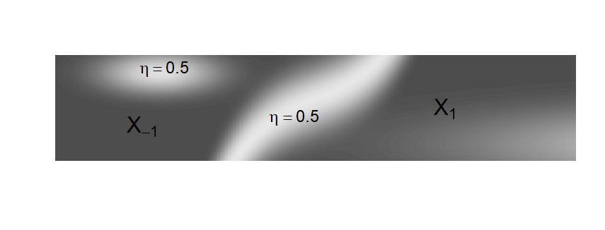
  • [9] [author] Steinwart, I.I. (2015). Fully adaptive density-based clustering. Ann. Statist. 43 2132–2167. 3396981
  • [10] [author] Steinwart, I.I. and Christmann, A.A. (2008). Support Vector Machines. Springer. 2450103