Phenomenological study of extended seesaw model for light sterile neutrino
Abstract
We study the zero textures of the Yukawa matrices in the minimal extended type-I seesaw (MES) model which can give rise to eV scale sterile neutrinos. In this model, three right handed neutrinos and one extra singlet are added to generate a light sterile neutrino. The light neutrino mass matrix for the active neutrinos, , depends on the Dirac neutrino mass matrix (), Majorana neutrino mass matrix () and the mass matrix () coupling the right handed neutrinos and the singlet. The model predicts one of the light neutrino masses to vanish. We systematically investigate the zero textures in and observe that maximum five zeros in can lead to viable zero textures in . For this study we consider four different forms for (one diagonal and three off diagonal) and two different forms of containing one zero. Remarkably we obtain only two allowed forms of ( and ) having inverted hierarchical mass spectrum. We re-analyze the phenomenological implications of these two allowed textures of in the light of recent neutrino oscillation data. In the context of the MES model, we also express the low energy mass matrix, the mass of the sterile neutrino and the active-sterile mixing in terms of the parameters of the allowed Yukawa matrices. The MES model leads to some extra correlations which disallow some of the Yukawa textures obtained earlier, even though they give allowed one-zero forms of . We show that the allowed textures in our study can be realized in a simple way in a model based on MES mechanism with a discrete Abelian flavor symmetry group .
1 Introduction
Neutrino oscillation experiments have established the fact that neutrinos have tiny mass and they change from one flavor to another during their propagation. This requires the Standard Model (SM) of particle physics to be extended in order to generate their masses. The standard 3-flavor neutrino oscillation scenario has six key parameters. These are the two mass squared differences ( ) which control the oscillations of the solar and atmospheric neutrinos respectively, three mixing angles () and a Dirac CP phase, . Global analysis of three flavor neutrino oscillation data from [1, 2, 3] give us the best fit values and the allowed ranges of these parameters. In 3-flavor paradigm, there are two more CP violating phases if neutrinos are Majorana particles. But as Majorana phases do not appear in the neutrino oscillation probability, they are not measurable in the oscillation experiments. Apart from these phases another major unknown is the absolute value of the neutrino mass since oscillation experiments are only sensitive to the mass squared differences. Planck data provide an upper bound on sum of neutrino masses to be eV [4] at 95% C.L. The sensitivity for the neutrino masses in the upcoming Karlsruhe Tritium Neutrino experiment (KATRIN) is expected to be around 200 meV (90% C.L.) [5].
Another interesting aspect of neutrino oscillation experiments is the search for the existence of a light sterile neutrino. As sterile neutrinos are SM singlets they do not take part in the weak interactions. But they can mix with the active neutrinos. Therefore, sterile neutrinos can be probed in neutrino oscillation experiments. The oscillation results from LSND experiment showed the evidence of at least one sterile neutrino having mass in the eV scale [6, 7, 8]. The latest data of MiniBooNE experiment [9] also have some overlap with the allowed regions of the LSND experiment and hence support the existence of the sterile neutrino hypothesis. The recently observed Gallium anomaly can also be explained by the sterile neutrino hypothesis [10]. Another evidence of eV sterile neutrino comes from the reactor antineutrino flux studies. This shows the deficit in the observed and predicted event rate of electron antineutrino flux and the ratio is at 98.6% C.L. [11]. Recent analysis of the Planck data shows the possibility of light sterile neutrino in the eV scale if one deviates slightly from the base CDM model [4]. In short, the scenario with a light sterile neutrino is quite riveting at present and many future experiments are proposed to confirm/falsify this [12]. Although it is possible to have a better fit of neutrino oscillation data with more than one light sterile neutrino [13, 14, 15], the 3+1 scheme i.e., three active neutrinos and one sterile neutrino in the sub-eV and eV scale respectively, is considered to be minimal. There are three different ways to add sterile neutrino in SM mass patterns and these are, (i) 3+1 scheme in which three active neutrinos are of sub-eV scale and sterile neutrino is of eV scale [16, 17], (ii) 2+2 scheme in which two different pairs of neutrino mass states differ by eV2 but this scheme was disfavored by solar and atmospheric data [18], and (iii) 1+3 scheme in which three active neutrinos are in eV scale and sterile neutrino is lighter than active neutrinos. This scenario is however disfavored from cosmology [19, 20]. Hence, we focus on the 3+1 scenario in our study.
Flavor symmetry models giving rise to eV sterile neutrinos have been studied in the literature [21, 22, 23]. These models might require modifications to usual seesaw framework [24, 25]. In the explicit seesaw models the eV scale sterile neutrinos with their mass suppressed by Froggatt - Nielsen mechanism can be naturally accommodated in non Abelian flavor symmetry [22, 26, 27]. bimodel or schizophrenic models for light sterile neutrinos are also widely studied [28, 29]. In order to have a theoretical understanding of the origin of eV sterile neutrino as well as admixtures between sterile and active neutrinos, the authors of Refs. [22, 26, 27] have studied an extension to the canonical type-I seesaw model. This model is known as “minimal extended type - I seesaw" (MES) model. In the MES model a fermion singlet, , is added along with three right handed neutrinos. This extension results into an eV scale sterile neutrino naturally, without imposing tiny mass scale or Yukawa term for this neutrino.
In this paper, for the first time we study the various possible textures of the Dirac neutrino mass matrix, , Majorana neutrino mass matrix, and the mass matrix that originate from the Yukawa interaction between right handed neutrinos with the gauge singlet within the framework of MES model and classify the allowed possibilities. Several papers have studied the consequences of imposing zeros in the neutrino mass matrix in standard three neutrino [30, 31, 32, 33, 34, 35, 36, 37, 38, 39, 40] and the 3+1 framework [41, 42, 43, 44, 45]. The more natural study would be to explore the zeros in the Yukawa matrices that appear in the Lagrangian rather than light neutrino mass matrix, . It has been noted by many authors [46, 47, 48, 49, 50] that the zeros of the Dirac neutrino mass matrix and the right handed Majorana mass matrix are the progenitors of zeros in the effective Majorana mass matrix through type - I seesaw mechanism. We also seek extra correlations connecting the parameters of the active and sterile sector which can put further constraints on the allowed possibilities. This motivates us to look for zeros in various neutrino mass matrices in the MES model which can lead to viable texture zeros in neutrino mass matrix.
We classify different structures of , and that can give allowed textures for the light neutrino mass matrix . Interestingly the only allowed form of that we obtain are the two one zero textures – namely and which are phenomenologically allowed and have the inverted hierarchical mass spectrum. For a originating from ordinary seesaw mechanism both these textures are viable. However, in the MES model, because of extra correlations connecting active and sterile sector, not all Yukawa matrices that give or for are allowed. We study these additional correlations and tabulate the allowed textures. We also include a discussion on the impact of NLO corrections in this model. In this context it is also important to study the origin of zero textures. Here, we show that it is possible to obtain various zero entries in lepton mass matrices with an Abelian discrete symmetry group . An alternative approach to obtain lepton mixing is discussed in [51] by considering non-Abelian symmetry group. We follow the method discussed in [52] to obtain Abelian discrete symmetry group which can generate viable zero textures in . Their method is based on type - I seesaw and we extend it to apply on MES model.
The paper is organized in the following manner. In the next section a brief review of the MES model is given. In Section 3 and its subsections we list the various forms of , and that lead to viable textures in . In Section 4 we discuss the implication of the allowed forms of one zero textures in obtained in Section 3. The following Section 5 discusses the results obtained from the comparison of low energy and high energy neutrino mass matrices and the extra correlations connecting active and sterile sector. Symmetry realizations for the allowed zero textures are discussed in Section 6. The summary of our findings and conclusions are presented in Section 7.
2 Minimal extended type I seesaw mechanism
In this section we describe the basic structure of MES model. Here, the fermion content of the SM is extended by three right handed neutrinos together with a gauge singlet field . One can get a natural eV-scale sterile neutrino without inserting any small Yukawa coupling in this model [22, 26]. The Lagrangian containing the neutrino masses is given by,
| (1) |
Here, are the () Dirac and Majorana mass matrices respectively and is a () coupling matrix between right handed neutrinos with the gauge singlet. In the basis (), the () neutrino mass matrix can be expressed as,
| (2) |
Considering the hierarchical mass spectrum of these mass matrices i.e. , in analogy of type - I seesaw, the right handed neutrinos are much heavier compared to the electroweak scale and thus they will decouple at the low scale. Therefore, Eq.(2) can be block diagonalized using seesaw mechanism and the effective neutrino mass matrix in the basis () can be written as,
| (3) |
Note that the rank of is three (see [26]) and hence one of the light neutrino remains massless.
Considering the case that , one can apply seesaw approximation once again on Eq.(3) to obtain the active neutrino mass matrix as11 1 Note that RHS of Eq.(4) does not vanish since is a vector rather than a square matrix.,
| (4) |
whereas the mass of the sterile neutrino is given by,
| (5) |
Note that the zero textures of fermion mass matrices in the context of type - I seesaw mechanism studied in [46, 47, 48, 50], leading to viable texture zeros in can be different from that of MES model because of the presence of the first term of Eq.(4). The active-sterile neutrino mixing matrix is given by,
| (6) |
where governs the strength of active-sterile mixing and can be expressed as,
| (7) |
Essentially, is suppressed by the ratio . Additionally in our formalism we assume , which is allowed by the current active sterile neutrino mixing data.
As the sterile neutrino mass ( eV) is heavier than active neutrinos, therefore, the mass pattern in the active sector can be arranged in two different ways. We denote 3+1 scenario as (SNH) when the three active neutrinos follow normal hierarchy () and the second choice is (SIH) when the three active neutrinos follow inverted hierarchy ) as shown in Fig(1). These masses can be expressed in terms of the mass squared differences obtained from oscillation experiments as given in Table(1).
| SNH | SIH | |
|---|---|---|
| 0 | ||
| 0 | ||
The best fit values along with 3 ranges of neutrino oscillation parameters used in our numerical analysis are given in Table(2).
| Parameter | Best Fit | Range |
|---|---|---|
| 7.37 | 6.93 – 7.97 | |
| (NH) | 2.50 | 2.37 – 2.63 |
| (IH) | 2.46 | 2.33 – 2.60 |
| 2.97 | 2.50 – 3.54 | |
| (NH) | 2.14 | 1.85 – 2.46 |
| (IH) | 2.18 | 1.86 – 2.48 |
| (NH) | 4.37 | 3.79 – 6.16 |
| (IH) | 5.69 | 3.83 – 6.37 |
| (NH) | 1.35 | 0 – 2 |
| (IH) | 1.32 | 0 –2 |
| (NH) | 0.0295 | 0.0263 – 0.0336 |
| (IH) | 0.0299 | 0.0266 – 0.0342 |
| 1.63 | 0.87 – 2.04 | |
| 0.027 | 0.012 – 0.047 | |
| 0.013 | 0.005 – 0.03 | |
| – | 0.16 |

In the next section we systematically explore the various zero texture structures of , and which can give rise to viable zero textures of .
3 Formalism
In our formalism, the charge lepton mass matrix, , is considered
to be diagonal.
For the right handed Majorana neutrino mass matrix,
we consider four different structures:
(i) Diagonal having three zeros i.e.,
| (8) |
(ii) non-diagonal minimal form of having four zeros with Det i.e.,
| (9) |
These three non-diagonal forms of correspond to , and flavor symmetry respectively. Such forms of in the context of zero textures in type-I seesaw model have been considered for instance in [56]. being a matrix can have one zero or two zeros. In [26], an based model was considered with 2 zeros in and 3 zeros in to obtain the as given by Eq. (4). But, in our analysis we find that mass matrices with 5 zeros in and two zeros in do not lead to any viable textures in . The only allowed possibility therefore is one zero in result in three possible structures. We find that the maximum number of zeros of that can give phenomenologically allowed zero textures in is five. The possible combinations of , and that lead to phenomenologically viable textures of are discussed in the following subsections.
3.1 5 zeros in and diagonal
First let us assume to be diagonal. As is a non-symmetric matrix, 5 zeros can be arranged in ways. Thus considering 126 cases of together with 3 cases of and 1 case of , we obtain total 378 possible structures of . Out of all possible combinations of these matrices the only allowed texture that we obtain is the one zero texture in with . Here, we have three possible forms of and these are,
| (10) |
The various forms of which lead to viable texture are presented below:
| (11) |
| (12) |
| (13) |
Here, , and are the permutation matrices that exchange first and second columns, first and third columns and second and third columns respectively. Therefore, we observe that out of 126 cases only 12 above forms of give the allowed texture of when is diagonal
3.2 5 zeros in and non-diagonal corresponding to flavor symmetry
The form of that we consider here corresponds to flavor symmetry as given in Eq.(9). Among the 378 possibilities we obtain two allowed one zero textures of , namely and . We observe that out of total 126 forms of , only four structures give rise to while eight structures give rise to . We list them below:
3.2.1 Textures leading to
| (14) |
3.2.2 Textures leading to
3.3 5 zeros in and non-diagonal corresponding to flavor symmetry
The form of that we consider in this subsection corresponds to flavor symmetry as given in Eq.(9). In this case also we observe that out of total 126 cases of , only four structures of give rise to and eight forms of give rise to texture . We list them below. Note that these forms of are different from those obtained in the earlier subsection.
3.3.1 Textures leading to
| (43) |
3.3.2 Textures leading to
3.4 5 zeros in and non-diagonal corresponding to flavor symmetry
The form of that we consider here corresponds to flavor symmetry as given in Eq.(9). Here also we observe that out of 126 cases of only four structures of give rise to texture and 8 forms of give rise to texture . But these forms of are different from those obtained in the earlier two subsections:
3.4.1 Structures leading to
| (72) |
3.4.2 Structures leading to
Note that in general the entries of the Yukawa matrices , and are complex (of the form ). However some of the phases can be absorbed by redefinition of the leptonic fields. For the case when is diagonal, the number of un-absrobed phases is two – one each in and whereas for the off-diagonal only one phase remains in . In this section we do not explicitly write the phases. However in section 5 where we discuss specific cases, the phases are explicitly included.
4 Active neutrino mass matrix with one zero texture
The () light neutrino mass matrix being symmetric, there are 6 possible cases of one zero textures with a vanishing lowest mass and these are studied in details in Refs. [57, 58, 59, 60]. In the above section we observed that in context of MES model only viable textures of that we obtain are and . According to the recent studies [59, 60, 61], both these textures are ruled out for normal hierarchy when the lowest mass is zero but they can be allowed for the inverted hierarchy even when then lowest mass is zero 22 2 We also observed that both these textures are disallowed for NH with the most recent data.. This kind of mass pattern can be obtained completely from group theoretical point of view if one assumes that Majorana neutrino mass matrix displays flavor antisymmetry under some discrete subgroup of SU(3) as discussed in [62, 63]. In this section we re-analyse the textures and for the inverted hierarchical mass spectrum assuming in the light of recent neutrino oscillation data as given in Table(2). In our analysis we find that correlations among various oscillation parameters become highly constrained as compared to the earlier studies. This is due to the recent constraints on the 3 ranges of the mass squared differences and as compared to earlier results in [58, 59, 60] 33 3 The latest constraint on comes from T2K and NOA including both appearance and disappearance modes [64, 65, 66, 67]. Whereas reanalysis of KamLAND data shows decrease in the value of and as discussed in [3]. .
In three neutrino paradigm, low energy Majorana neutrino mass matrix can be diagonalized as,
| (101) |
Here, () is a lepton mixing matrix in the basis where is diagonal. The Pontecorvo-Maki-Nakagawa-Sakata (PMNS) matrix has 3 mixing angles and a CP violation phase .
The elements of neutrino mass matrix can be calculated from Eq.(101) are,
| (102) |
where, and are given in Table(1). We express elements of as in the text.
Imposing the condition of zero texture for IH with in the above equation we get,
| (103) |
which can be simplified to obtain the mass ratio
| (104) |
Let, we get
| (105) | ||||
| (106) |
Let us define the ratio of the two mass squared differences as,
| (107) |
The defined above can be calculated either using the current neutrino mass squared differences as given in Table(2) or by calculating . If the value of calculated using falls in the allowed range of from the current data, then we say the texture under consideration is allowed by the current data. As given in Table(2) we vary the Dirac CP phase from 0∘ 360∘ while the relevant Majorana phase in the range 0∘ 180∘ and find the correlations among different parameters, specially the predictions for and .
We also study the effective Majorana neutrino mass, , governing neutrinoless double beta decay () for these allowed textures. In three flavor paradigm this can be written as,
| (108) |
where ). From the above equation we understand that depends on the Majorana phases but not on the Dirac phase. Various experiments such as CUORE [68], GERDA [69], SuperNEMO [70], KamLAND-ZEN [71] and EXO [72] are looking for signatures for neutrinoless double beta decay (). The current experiments provide bounds on the effective Majorana mass from the non-observation of . For instance, the combined results from KamLAND-ZEN and EXO-200 [71] give the upper bound on the effective Majorana neutrino mass as (0.12 - 0.25) eV where the range signifies the uncertainty in the nuclear matrix elements. The future experiments can improve this limit by one order of magnitude. Below we discuss the various correlations that we obtain for the allowed textures.
4.1 Case I:


The Majorana mass matrix element in 3-flavor case can be written as,
| (109) |
Imposing the condition of zero texture with vanishing lowest mass () for IH, we get,
| (110) | |||
| (111) |
From the above equation we obtain the mass ratio as below
| (112) |
The mass ratio should be greater than 1. For this to happen should be negative. We find that due to the interplay of the terms and the phase is restricted to the range and . The effective mass, as function of Majorana phase is constrained due to very small allowed range of (5 10∘, 170 175∘) as shown in Eq(108). The allowed range of for this texture is 0.046 eV 0.05 eV and which can be probed in future experiments. Also, this texture predicts Dirac CP phase which is in agreement with the indications from the current ongoing oscillation experiments like T2K and NOA. There is however no constrain on the values of the neutrino mixing angles and seen in right panel of Fig.2 for this texture.
4.2 Case II:
The Majorana mass matrix element in 3-flavor case can be written as,
| (113) |
Imposing the condition of texture zero with vanishing lowest mass() for IH, we get,
| (114) | |||
| (115) |
The mass ratio from the above equation can be written as
| (116) |


Since this mass ratio is always greater than 1 from oscillation data, we find that should be negative for this texture as well. As can be seen from Fig 3 that is constrained in the range . We observe that, due to the more constrained values of mass squared differences and from present data, as considered in our analysis, the atmospheric mixing angle is restricted to be below maximal. In the earlier analysis [58, 59, 60] there was no preferred octant of . The values of 45∘ are disallowed for this texture as can be seen in Fig 3. The effective mass, , being function of unknown Majorana phase as seen in Eq(108) is constrained due to very small allowed range of (80110∘). The allowed range of for this texture is 0.014 eV 0.018 eV which is smaller compared to the case =0 where a vanishing element is off-diagonal. The allowed values of the effective mass for diagonal texture are on the lower side having no overlap with non diagonal texture zero . Thus, can be used to distinguish between diagonal and off-diagonal one texture zero classes with a vanishing neutrino mass. Note that allowed ranges of and are more constrained in our analysis as compared to references [58, 59] again due to the recent improved constraints on the mass squared differences and at 3.
5 Comparison of low and high energy neutrino mass matrix elements
In this section we obtain the light neutrino neutrino mass matrix () (Eq.4), sterile mixing matrix () (Eq.5) and the active sterile mixing matrix (R) (Eq.7) using the different forms of , and given in section (III) of the MES model. Since in the MES model both the active neutrino mass matrix and the active sterile mixing matrix depends on the parameters of , and , this can induce additional correlations between active and sterile sector. Similarly, the mass of the sterile neutrino depends on and . Hence expressing the various variables in terms of the parameters of these matrices one can get some interrelations.
For an illustration we will discuss three specific cases. In case I and II we discuss assuming diagonal structure of and in the case III we talk about by considering the off diagonal form of . Note that here we consider the complex phases in our calculation. We compare high energy mass matrix with low energy mass matrix after the decoupling of the eV sterile neutrino as discussed in section II.
- •
Case I : Considering the forms of , and diagonal from Eq.(11),
(117) and using them in Eqs(4, 5 and 7) we get the low energy neutrino mass matrix, the sterile mass and the active sterile mixing matrix as,
From Eq.(• ‣ 5) and (• ‣ 5) it can be seen that
Here are the low energy neutrino mass matrix elements. The eigen values of will give the masses of the three active neutrinos. Note that, only allowed hierarchy in our case is IH and hence and . From Eq.(• ‣ 5) we get,
(128) We find that the lhs of Eq.(128) lies in the range (0.63 – 3.06) whereas rhs lies in (3.9 - 5.9) in their 3 range. This shows that there is no overlapping between lhs and rhs of Eq.(128) and hence disallowed from current neutrino oscillation data. We observe that out of 12 forms of as given in Eq.(11 -13), 6 of them (, , , , and ) do not lead to the correlation given in Eq.(128) and these ’s are not ruled out. Hence a detail analysis of one of these ’s is discussed below in Case II.
- •
Case II : Considering the form of , and diagonal given in Eq.(11),
(129) and using them in Eqs(4, 5 and 7) we get the texture ,
The sterile mass and active sterile mixing becomes
It can be seen from the above equations that
(139) From Eq.(• ‣ 5) we get the following relation between the light neutrino mass matrix elements,
which implies,
(140) To obtain Eq.(140) we have used the correlations of Eq.(139). Now to test the viability of these structures of , and , we look for the parameter space in which both the conditions and Eq.(140) are satisfied simultaneously. In the upper panels of Fig. 4, we have plotted the correlations obtained between different low energy parameters in this scenario. Comparing these correlations with Fig. 2 (which corresponds to only ), we find that the MES model disfavours a large area in the plane and allows values in the lower octant : whereas the admissible values of ( ) are near the higher side of it’s allowed range. However the values of and which are predicted by the two cases are similar. The prediction of the texture with is and while the MES model predicts a slightly constrained range and . In this case we also obtain another correlation for sterile neutrino mass from this model of the form,
(141) 


Figure 4: Correlation plots for case II. In the lower panels of Fig.4, we have plotted the prediction of as given by Eq.(141) by varying and within their allowed range as given in table(2). This is obtained when both the conditions i.e., and Eq.(140) is satisfied simultaneously. From the figures we see that the prediction of by this model is consistent with data coming from the SBL experiments.
- •
Case III : Considering the cases for the off-diagonal forms of given in Eqs.(14-3.4.2), we find that out of the 36 , 19 cases lead to exactly the same correlation depicted by Eq.(128). This is not allowed from current oscillation data as discussed earlier. Among the remaining 17 cases 11 (for and ) lead to a correlation of the form,
(142) This is also not satisfied by current neutrino oscillation data as the rhs of Eq.(142) lies in the range (3.8 – 4.7) showing no overlapping with lhs. The remaining six forms of are , , , , and . All these forms of and the corresponding forms of and lead to neutrino mass matrix with . We found that, all these ’s lead a correlation of the form,
(143) which is satisfied by current oscillation data. The rhs of Eq.(142) lies in the range (1.8 – 2.3) which shows complete overlap with lhs (0.63- 3.06). For illustration, we consider with corresponding and and using them in Eqs(4, 5 and 7) we get ,
From the above matrices we find the following correlation,
(153) also the correlation mentioned by Eq.(143). We find that both the equations (143 and 153) are consistent with the current oscillation data. The simultaneous validity of equations (143 and 153) lead to light sterile neutrino mass in the range which is marginally allowed by global analysis as seen from Fig.(5). However, individual experiments (MINOS, IceCube, Daya Bay) still allow higher value of sterile neutrino mass [73, 74, 75, 76].


In Table(3) and Table(4) we summarize the allowed cases that we obtained in our study for texture and respectively.
| Case | Correlations | |||
|---|---|---|---|---|
| I | diag() | |||
| II | diag() | Same as Case I | ||
| III | diag() | Same as Case I | ||
| IV | diag() | Same as Case I | ||
| V | diag() | Same as Case I | ||
| VI | diag() | Same as Case I |
| Case | Correlations | |||
|---|---|---|---|---|
| I | ||||
| II | Same as Case I | |||
| III | Same as Case I | |||
| IV | Same as Case I | |||
| V | Same as Case I | |||
| VI | Same as Case I |
5.1 NLO correction for MES model
In sec.(3), the structures of various mass matrices are obtained using the leading order expression of as given by equation (4) which give rise to texture zeros with exact cancellation. However, if NLO corrections can be important. In this section, we discuss the effect of NLO correction terms for MES model corresponding to the allowed texture zeros. The NLO correction term can be calculated following the standard algorithm given in [77]. To calculate the NLO term, let us rewrite equation (3) in the form,
| (154) |
where,
| (155) |
| (156) |
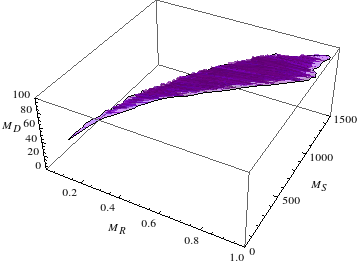
In the second line we use the form of and as given by equation (155) to obtain the final form given by equation (156). We see that the contribution of the NLO terms of equation (156) are proportional to . This implies that a term of the order will add to every term of as given by the equation (• ‣ 5). To get the specific form of NLO correction term, in equation (156), we use the specific forms of , and used for obtaining equation (• ‣ 5). The NLO correction term we obtain for (1,3) element of equation (• ‣ 5) is , which is of the order of , where are elements of , are elements of and are elements of . We see here that because of NLO corrections, we no longer have exact cancellation leading to , unlike the leading order case. But, if we consider representative values of parameters say, GeV, GeV and GeV then we find that eV, eV, R and NLO eV. In figure (6) we show the allowed parameter spaces of , and which can lead to NLO correction term eV or less.44 4 In our numerical analysis texture zero (say, ) corresponds to . Hence, there exist a parameter space where we can safely neglect NLO correction terms in our analysis compared to leading order terms and consider the texture zero even with the inclusion of the NLO term.55 5 We notice that the set of , and which do not give NLO eV do not give the one zero textures. Thus, all the model predictions corresponding to leading order terms remain unchanged. Note that similar conclusions can also be obtained for the texture .
6 Symmetry realization
Singular one zero neutrino mass matrices can be realized using a discrete Abelian flavor symmetry within the context of MES mechanism. Earlier in [52] authors studied the possibilities to enforce zero textures in arbitrary entries of the fermion mass matrices by means of Abelian symmetries in the context of type - I seesaw mechanism. We adopt the same approach to probe the zero textures of in the context of MES mechanism. We observe that one zero textures of with a vanishing mass can be realized by symmetry. To realize the texture structures we extend the SM particle composition by three right handed neutrinos (, , ) as required in MES model and two more Higgs doublets (, ) in addition to the SM one (). Few scalar singlets (, ) are required to realize diagonal whereas two singlets , helps in realizing one zero texture structure of . Note that the model that we discuss here to get the zero texture structure is general, flexible and in no way unique. The additional discrete group is introduced to restrict some of the unwanted terms in the Lagrangian. For illustration, we present the detailed symmetry realization of our two viable textures of . The particle assignments for which is allowed by current data (case II) under the action of symmetry are given in Table (5).
| Lepton | () | RH Singlet | () | fields | () | Higgs | () |
|---|---|---|---|---|---|---|---|
| doublet | doublet | ||||||
| (, -1) | (, -1) | (, 1) | (1, 1) | ||||
| (, 1) | (, 1) | (, -1) | (, 1) | ||||
| (, 1) | (1, 1) | (1, 1) | (, 1) |
According to the charge assignments of the leptonic field given in Table (5) the bilinears , and relevant for , and transform as,
, , ,
where . We introduce three doublet Higgs (,). One of these Higgs doublet , is invariant under while the other two fields transforms as: () and (). The () invariant Yukawa Lagrangian than becomes
| (157) | ||||
here all . The Higgs fields acquires the vacuum expectation values and results in the and of the following form,
| (158) |
Here , . The elements of are , , and . For the right-handed Majorana mass matrix () and for the mass matrix , we introduce few scalar singlets and their transformation under is given in the Table(6).
| Scalar singlet | () | Scalar singlet | () |
|---|---|---|---|
| (, 1) | (1, 1) | ||
| (, 1) | (, -1) |
Thus the mass matrices and becomes,
| (159) |
We also give the transformation to the singlet field S as (, -1) under () which will prevent the term of the form as demand by the MES model will still give the correct form of .
Using the minimal extended type I seesaw given in Eqn (4) with the mass matrices , and as discussed above leads to effective neutrino mass matrix with a texture zero at (1,3) position.
| Lepton | () | RH Singlet | () | fields | () | Higgs | () |
|---|---|---|---|---|---|---|---|
| doublet | doublet | ||||||
| (1, 1) | (1, 1) | (, 1) | (1, 1) | ||||
| (, -1) | (, -1) | (, 1) | (, 1) | ||||
| (, 1) | (, 1) | (1, -1) |
Similarly, one can assign the various fields transformation under the action of () to obtain the texture with . The form of , and used to get are given in Eq.(3.2.2). We summarize the fields transformations in the Table 7. Here, no extra scalar singlet is needed to obtain the mass structure of which has symmetry and for we need two scalar singlets (, ) which transform under as (, 1) and (, -1) respectively. We also give transformation to singlet field S as (, 1) under () which will prevent the term . Note that symmetry realization of this texture is more economical than the texture.
7 Conclusions
In this paper we have studied the low energy phenomenology of the minimal extended type I seesaw model which can accommodate an eV scale light sterile neutrino [22, 26]. This model is motivated by the recent experimental evidences which support the existence of light sterile neutrinos in addition to three active neutrinos. In this model, apart from three right handed neutrinos, an extra gauge singlet is added to the SM. Under the minimal extended seesaw mechanism, this model give rise to three active neutrinos in the sub-eV scale with one of the active neutrinos having vanishing mass and one sterile neutrino in the eV scale. In this model the Dirac mass matrix, , is an arbitrary complex matrix, the Majorana mass matrix is a complex symmetric matrix and which couples the right handed neutrinos and the singlet is a matrix.
We obtain different textures of , and that give rise to phenomenologically allowed zero textures in the low energy neutrino mass matrix, . The maximum number of zeros in that results in viable are found to be five. Thus, there are 126 different possible structures of to be probed. We consider four possible structures of with one diagonal and three non diagonal forms. The maximum number of zeros in is one as two zeros do not result in phenomenologically viable textures of . This leads to three possible structures of . After analyzing all the different combinations we obtain only two viable one zero textures of ( and ) with different possible structures of , and . We study these textures of in the light of the current oscillation data. Both these textures have inverted hierarchical mass spectrum and we get constraints on observables like effective Majorana neutrino mass and Dirac CP phase . For the texture , we obtain the allowed values of Dirac CP phase is around . Note that is favored by current neutrino oscillation experiments. For , lies between (150∘–240∘). The allowed range for the effective Majorana mass is different for both these textures. It can thus be used to distinguish between the two textures. Also, in our study we observed that due to improved constraints on the mass squared differences and the texture disfavours higher octant of .
Next we studied the predictions of the MES model for the Yukawa matrices that gave viable forms of and check whether any extra correlations can come from the model. This is expected since in the framework of this model both the active and sterile neutrino masses as well as the active sterile mixing depend on the parameters of the Yukawa matrices , and . Thus, there may be additional relations between different observables, which are the predictions of the model. We find that some of the Yukawa matrices which can generate allowed one zero textures and in the active neutrino mass matrix, , cannot satisfy the extra correlations coming from the predictions of the MES model. Our analysis reveals that due to these additional correlations among the possible combinations of , and , only 6 combinations giving and other 6 combinations giving are allowed from the current oscillation data. The 6 allowed combinations which give , reveal severe restrictions on the values of and due to the extra correlations in the MES model and only the lower octant of and relatively higher values of remains allowed. In addition an interesting correlation is obtained connecting the mass of the sterile neutrino to the active sterile mixing parameters which also involves the light neutrino masses and mixing. Thus this correlation connects the active and the sterile sector. For the prediction for the sterile neutrino mass obtained from the MES model is in complete agreement with what is obtained from global analysis. The texture, also predicts a correlation for sterile neutrino mass. This however is in marginal agreement with the global analysis. We also explored the consequences of NLO correction terms in our analysis and depicted the parameter space in , and for which the NLO corrections can be neglected as compared to the leading order term. Finally, working within the framework of MES mechanism, we present simple discrete Abelian symmetry models leading to the two phenomenologically allowed zero textures of .
In conclusion, we analyzed the low energy prediction of the minimal extended seesaw model that can give an eV scale sterile neutrino. We emphasize that this task is performed for the first time in this paper. The results described in our analysis shows the compatibility of this model to the neutrino oscillation data. We also find correlations that can be tested in future experiments. This kind of study is indispensable to test the viability of a given model in the context of present and forthcoming neutrino oscillation experiments.
Acknowledgements.
Authors are grateful to Anjan Joshipura for discussions and useful comments in the initial stages of the work. The work of SG is supported by the Australian Research Council through the ARC Center of Excellence for Particle Physics (CoEPP Adelaide) at the Terascale (CE110001004). The work of MG is supported by the “Grant-in-Aid for Scientific Research of the Ministry of Education, Science and Culture, Japan", under Grant No. 25105009.References
- (1) M. C. Gonzalez-Garcia, M. Maltoni, and T. Schwetz, Global Analyses of Neutrino Oscillation Experiments, arXiv:1512.0685.
- (2) D. V. Forero, M. Tortola, and J. W. F. Valle, Neutrino oscillations refitted, Phys. Rev. D90 (2014), no. 9 093006, [arXiv:1405.7540].
- (3) F. Capozzi, E. Lisi, A. Marrone, D. Montanino, and A. Palazzo, Neutrino masses and mixings: Status of known and unknown parameters, Nucl. Phys. B908 (2016) 218–234, [arXiv:1601.0777].
- (4) Planck Collaboration, P. A. R. Ade et al., Planck 2015 results. XIII. Cosmological parameters, arXiv:1502.0158.
- (5) S. Mertens, Status of the katrin experiment and prospects to search for kev-mass sterile neutrinos in tritium β-decay, Physics Procedia 61 (2015) 267 – 273.
- (6) LSND Collaboration, C. Athanassopoulos et al., Evidence for anti-muon-neutrino —> anti-electron-neutrino oscillations from the LSND experiment at LAMPF, Phys.Rev.Lett. 77 (1996) 3082–3085, [nucl-ex/9605003].
- (7) LSND Collaboration, C. Athanassopoulos et al., Evidence for nu(mu) —> nu(e) neutrino oscillations from LSND, Phys.Rev.Lett. 81 (1998) 1774–1777, [nucl-ex/9709006].
- (8) LSND Collaboration, A. Aguilar-Arevalo et al., Evidence for neutrino oscillations from the observation of anti-neutrino(electron) appearance in a anti-neutrino(muon) beam, Phys.Rev. D64 (2001) 112007, [hep-ex/0104049].
- (9) MiniBooNE Collaboration, A. A. Aguilar-Arevalo et al., Improved Search for Oscillations in the MiniBooNE Experiment, Phys. Rev. Lett. 110 (2013) 161801, [arXiv:1207.4809].
- (10) C. Giunti and M. Laveder, Statistical Significance of the Gallium Anomaly, Phys.Rev. C83 (2011) 065504, [arXiv:1006.3244].
- (11) G. Mention, M. Fechner, T. Lasserre, T. Mueller, D. Lhuillier, et al., The Reactor Antineutrino Anomaly, Phys.Rev. D83 (2011) 073006, [arXiv:1101.2755].
- (12) K. N. Abazajian et al., Light Sterile Neutrinos: A White Paper, arXiv:1204.5379.
- (13) J. Kopp, M. Maltoni, and T. Schwetz, Are there sterile neutrinos at the eV scale?, Phys. Rev. Lett. 107 (2011) 091801, [arXiv:1103.4570].
- (14) J. M. Conrad, C. M. Ignarra, G. Karagiorgi, M. H. Shaevitz, and J. Spitz, Sterile Neutrino Fits to Short Baseline Neutrino Oscillation Measurements, Adv. High Energy Phys. 2013 (2013) 163897, [arXiv:1207.4765].
- (15) C. Giunti and M. Laveder, 3+1 and 3+2 Sterile Neutrino Fits, Phys. Rev. D84 (2011) 073008, [arXiv:1107.1452].
- (16) J. J. Gomez-Cadenas and M. C. Gonzalez-Garcia, Future tau-neutrino oscillation experiments and present data, Z. Phys. C71 (1996) 443–454, [hep-ph/9504246].
- (17) S. Goswami, Accelerator, reactor, solar and atmospheric neutrino oscillation: Beyond three generations, Phys. Rev. D55 (1997) 2931–2949, [hep-ph/9507212].
- (18) M. Maltoni, T. Schwetz, M. A. Tortola, and J. W. F. Valle, Constraining neutrino oscillation parameters with current solar and atmospheric data, Phys. Rev. D67 (2003) 013011, [hep-ph/0207227].
- (19) J. Hamann, S. Hannestad, G. G. Raffelt, I. Tamborra, and Y. Y. Y. Wong, Cosmology seeking friendship with sterile neutrinos, Phys. Rev. Lett. 105 (2010) 181301, [arXiv:1006.5276].
- (20) E. Giusarma, M. Corsi, M. Archidiacono, R. de Putter, A. Melchiorri, O. Mena, and S. Pandolfi, Constraints on massive sterile neutrino species from current and future cosmological data, Phys. Rev. D83 (2011) 115023, [arXiv:1102.4774].
- (21) E. J. Chun, A. S. Joshipura, and A. Yu. Smirnov, QuasiGoldstone fermion as a sterile neutrino, Phys. Rev. D54 (1996) 4654–4661, [hep-ph/9507371].
- (22) J. Barry, W. Rodejohann, and H. Zhang, Light Sterile Neutrinos: Models and Phenomenology, JHEP 1107 (2011) 091, [arXiv:1105.3911].
- (23) C.-S. Chen and R. Takahashi, Hierarchically Acting Sterile Neutrinos, Eur. Phys. J. C72 (2012) 2089, [arXiv:1112.2102].
- (24) A. de Gouvea, J. Jenkins, and N. Vasudevan, Neutrino Phenomenology of Very Low-Energy Seesaws, Phys. Rev. D75 (2007) 013003, [hep-ph/0608147].
- (25) P. S. Bhupal Dev and A. Pilaftsis, Light and Superlight Sterile Neutrinos in the Minimal Radiative Inverse Seesaw Model, Phys. Rev. D87 (2013), no. 5 053007, [arXiv:1212.3808].
- (26) H. Zhang, Light Sterile Neutrino in the Minimal Extended Seesaw, Phys. Lett. B714 (2012) 262–266, [arXiv:1110.6838].
- (27) J. Heeck and H. Zhang, Exotic Charges, Multicomponent Dark Matter and Light Sterile Neutrinos, JHEP 05 (2013) 164, [arXiv:1211.0538].
- (28) R. Allahverdi, B. Dutta, and R. N. Mohapatra, Schizophrenic Neutrinos and -less Double Beta Decay, Phys. Lett. B695 (2011) 181–184, [arXiv:1008.1232].
- (29) A. C. B. Machado and V. Pleitez, Schizophrenic active neutrinos and exotic sterile neutrinos, Phys. Lett. B698 (2011) 128–130, [arXiv:1008.4572].
- (30) S. Dev, S. Kumar, S. Verma, and S. Gupta, Phenomenology of two-texture zero neutrino mass matrices, Phys.Rev. D76 (2007) 013002, [hep-ph/0612102].
- (31) Z.-z. Xing, Texture zeros and Majorana phases of the neutrino mass matrix, Phys.Lett. B530 (2002) 159–166, [hep-ph/0201151].
- (32) Z.-z. Xing, A Full determination of the neutrino mass spectrum from two zero textures of the neutrino mass matrix, Phys.Lett. B539 (2002) 85–90, [hep-ph/0205032].
- (33) B. R. Desai, D. Roy, and A. R. Vaucher, Three neutrino mass matrices with two texture zeros, Mod.Phys.Lett. A18 (2003) 1355–1366, [hep-ph/0209035].
- (34) S. Dev, S. Kumar, S. Verma, and S. Gupta, CP violation in two texture zero neutrino mass matrices, Phys.Lett. B656 (2007) 79–82, [arXiv:0708.3321].
- (35) S. Dev, S. Kumar, S. Verma, and S. Gupta, Phenomenological implications of a class of neutrino mass matrices, Nucl.Phys. B784 (2007) 103–117, [hep-ph/0611313].
- (36) S. Kumar, Implications of a class of neutrino mass matrices with texture zeros for non-zero , Phys.Rev. D84 (2011) 077301, [arXiv:1108.2137].
- (37) H. Fritzsch, Z.-z. Xing, and S. Zhou, Two-zero Textures of the Majorana Neutrino Mass Matrix and Current Experimental Tests, JHEP 1109 (2011) 083, [arXiv:1108.4534].
- (38) D. Meloni and G. Blankenburg, Fine-tuning and naturalness issues in the two-zero neutrino mass textures, Nucl.Phys. B867 (2013) 749–762, [arXiv:1204.2706].
- (39) P. Ludl, S. Morisi, and E. Peinado, The Reactor mixing angle and CP violation with two texture zeros in the light of T2K, Nucl.Phys. B857 (2012) 411–423, [arXiv:1109.3393].
- (40) W. Grimus and P. Ludl, Two-parameter neutrino mass matrices with two texture zeros, J.Phys. G40 (2013) 055003, [arXiv:1208.4515].
- (41) M. Ghosh, S. Goswami, and S. Gupta, Two Zero Mass Matrices and Sterile Neutrinos, JHEP 04 (2013) 103, [arXiv:1211.0118].
- (42) M. Ghosh, S. Goswami, S. Gupta, and C. S. Kim, Implication of a vanishing element in the 3+1 scenario, Phys. Rev. D88 (2013), no. 3 033009, [arXiv:1305.0180].
- (43) Y. Zhang, Majorana neutrino mass matrices with three texture zeros and the sterile neutrino, Phys.Rev. D87 (2013), no. 5 053020, [arXiv:1301.7302].
- (44) N. Nath, M. Ghosh, and S. Gupta, Understanding the masses and mixings of one-zero textures in 3 + 1 scenario, Int. J. Mod. Phys. A31 (2016), no. 24 1650132, [arXiv:1512.0063].
- (45) D. Borah, M. Ghosh, S. Gupta, S. Prakash, and S. K. Raut, Analysis of four-zero textures in framework, arXiv:1606.0207.
- (46) G. C. Branco, D. Emmanuel-Costa, M. N. Rebelo, and P. Roy, Four Zero Neutrino Yukawa Textures in the Minimal Seesaw Framework, Phys. Rev. D77 (2008) 053011, [arXiv:0712.0774].
- (47) S. Goswami and A. Watanabe, Minimal Seesaw Textures with Two Heavy Neutrinos, Phys. Rev. D79 (2009) 033004, [arXiv:0807.3438].
- (48) S. Goswami, S. Khan, and A. Watanabe, Hybrid textures in minimal seesaw mass matrices, Phys. Lett. B693 (2010) 249–254, [arXiv:0811.4744].
- (49) S. Choubey, W. Rodejohann, and P. Roy, Phenomenological consequences of four zero neutrino Yukawa textures, Nucl. Phys. B808 (2009) 272–291, [arXiv:0807.4289]. [Erratum: Nucl. Phys.B818,136(2009)].
- (50) L. Lavoura, New texture-zero patterns for lepton mixing, J. Phys. G42 (2015) 105004, [arXiv:1502.0300].
- (51) R. M. Fonseca and W. Grimus, Classification of lepton mixing matrices from finite residual symmetries, JHEP 09 (2014) 033, [arXiv:1405.3678].
- (52) W. Grimus, A. S. Joshipura, L. Lavoura, and M. Tanimoto, Symmetry realization of texture zeros, Eur. Phys. J. C36 (2004) 227–232, [hep-ph/0405016].
- (53) S. Gariazzo, C. Giunti, M. Laveder, Y. F. Li, and E. M. Zavanin, Light sterile neutrinos, J. Phys. G43 (2016) 033001, [arXiv:1507.0820].
- (54) C. Giunti, Oscillations beyond three-neutrino mixing, 2016. Talk given at Proceedings of Neutrino 2016, London, UK.
- (55) T. Schwetz, Global oscillation fits with sterile neutrinos, 2011. Talk given at Proceedings of Sterile Neutrino Crossroads, 2011, Virginia Tech, USA.
- (56) S. Goswami, S. Khan, and W. Rodejohann, Minimal Textures in Seesaw Mass Matrices and their low and high Energy Phenomenology, Phys. Lett. B680 (2009) 255–262, [arXiv:0905.2739].
- (57) A. Merle and W. Rodejohann, The Elements of the neutrino mass matrix: Allowed ranges and implications of texture zeros, Phys. Rev. D73 (2006) 073012, [hep-ph/0603111].
- (58) E. I. Lashin and N. Chamoun, The One-zero Textures of Majorana Neutrino Mass Matrix and Current Experimental Tests, Phys. Rev. D85 (2012) 113011, [arXiv:1108.4010].
- (59) R. R. Gautam, M. Singh, and M. Gupta, Neutrino mass matrices with one texture zero and a vanishing neutrino mass, Phys. Rev. D92 (2015), no. 1 013006, [arXiv:1506.0486].
- (60) L. Lavoura, W. Rodejohann, and A. Watanabe, Reproducing lepton mixing in a texture zero model, Phys. Lett. B726 (2013) 352–355, [arXiv:1307.6421].
- (61) K. Harigaya, M. Ibe, and T. T. Yanagida, Seesaw Mechanism with Occam’s Razor, Phys. Rev. D86 (2012) 013002, [arXiv:1205.2198].
- (62) A. S. Joshipura, Neutrino masses and mixing from flavour antisymmetry, JHEP 11 (2015) 186, [arXiv:1506.0045].
- (63) A. S. Joshipura and N. Nath, Neutrino masses and mixing in with flavor antisymmetry, Phys. Rev. D94 (2016), no. 3 036008, [arXiv:1606.0169].
- (64) T2K Collaboration, K. Abe et al., Measurements of neutrino oscillation in appearance and disappearance channels by the T2K experiment with 6.6×10²⁰ protons on target, Phys. Rev. D91 (2015), no. 7 072010, [arXiv:1502.0155].
- (65) T2K Collaboration, M. Ravonel Salzgeber, Anti-neutrino oscillations with T2K, arXiv:1508.0615.
- (66) NOvA Collaboration, P. Adamson et al., First measurement of electron neutrino appearance in NOvA, Phys. Rev. Lett. 116 (2016), no. 15 151806, [arXiv:1601.0502].
- (67) NOvA Collaboration, P. Adamson et al., First measurement of muon-neutrino disappearance in NOvA, Phys. Rev. D93 (2016), no. 5 051104, [arXiv:1601.0503].
- (68) CUORE Collaboration, P. Gorla, The CUORE experiment: Status and prospects, J.Phys.Conf.Ser. 375 (2012) 042013.
- (69) J. Wilkerson, E. Aguayo, F. Avignone, H. Back, A. Barabash, et al., The MAJORANA demonstrator: A search for neutrinoless double-beta decay of germanium-76, J.Phys.Conf.Ser. 375 (2012) 042010.
- (70) SuperNEMO Collaboration, A. Barabash, SuperNEMO double beta decay experiment, J.Phys.Conf.Ser. 375 (2012) 042012.
- (71) KamLAND-Zen Collaboration, A. Gando et al., Limit on Neutrinoless Decay of 136Xe from the First Phase of KamLAND-Zen and Comparison with the Positive Claim in 76Ge, Phys.Rev.Lett. 110 (2013), no. 6 062502, [arXiv:1211.3863].
- (72) EXO Collaboration, M. Auger et al., Search for Neutrinoless Double-Beta Decay in 136Xe with EXO-200, Phys.Rev.Lett. 109 (2012) 032505, [arXiv:1205.5608].
- (73) Daya Bay Collaboration, F. P. An et al., Improved Search for a Light Sterile Neutrino with the Full Configuration of the Daya Bay Experiment, arXiv:1607.0117.
- (74) IceCube Collaboration, M. G. Aartsen et al., Searches for Sterile Neutrinos with the IceCube Detector, Phys. Rev. Lett. 117 (2016), no. 7 071801, [arXiv:1605.0199].
- (75) MINOS Collaboration, P. Adamson et al., A search for sterile neutrinos mixing with muon neutrinos in MINOS, Submitted to: Phys. Rev. Lett. (2016) [arXiv:1607.0117].
- (76) MINOS, Daya Bay Collaboration, P. Adamson et al., Limits on Active to Sterile Neutrino Oscillations from Disappearance Searches in the MINOS, Daya Bay, and Bugey-3 Experiments, Submitted to: Phys. Rev. Lett. (2016) [arXiv:1607.0117].
- (77) W. Grimus and L. Lavoura, The Seesaw mechanism at arbitrary order: Disentangling the small scale from the large scale, JHEP 11 (2000) 042, [hep-ph/0008179].