A Randomised Primal-Dual Algorithm for Distributed Radio-Interferometric ImagingThanks: This work was supported by the UK Engineering and Physical Sciences Research Council (EPSRC, grants EP/M011089/1 and EP/M008843/1) and by the UK Science and Technology Facilities Council (STFC, grant ST/M00113X/1), as well as by the Swiss National Science Foundation (SNSF) under grant 200020-146594.

Radio interferometry (RI) is a technique that, by measuring signal correlations between geographically separated antennas, is able to greatly improve the sensitivity and angular resolution with which we can observe radio emissions. Extensively studied, it provides valuable data driving many research directions in cosmology, astronomy, and astrophysics [1]. It has greatly contributed to the advancement of our understanding of the universe. In the future, the Square Kilometre Array, is expected to acquire massive amounts of data which will be used to reconstruct giga-pixel sized images, two orders of magnitude improvement over current instruments [2]. Under these big-data challenges, the methods solving the image reconstruction problem need be computationally efficient and to scale well in order to work with a huge number of measurements.

Recently, advances in sparse modelling and convex optimisation allowed the development of efficient algorithms able to outperform the standard RI methods in terms of both reconstruction quality and computational cost [3]. Modern optimisation techniques, like the proximal splitting and the primal-dual (PD) methods, are of particular importance since they decompose the main minimisation problem into multiple, simpler, subproblems for different data blocks or priors that are solved in parallel [4, 5].

Herein, we study a randomised algorithmic structure, based on the PD framework, for solving a sparse regularization problem in the context of RI imaging [6]. We review the algorithmic structure from [7] and present a new strategy for the choice of probabilities that significantly improves the convergence speed. The algorithm achieves the full splitting of the functions and operators used and has a highly parallelisable structure. The computational cost is much lower than that of the simultaneous direction method of multipliers (SDMM) [3], previously proposed for a similar problem. Through randomisation, the method achieves great flexibility, in terms of computational burden per iteration and memory load, at the cost of requiring more iterations to converge. An adaptive nonuniform choice for the probabilities provides an excellent tradeoff between complexity per iteration and convergence speed.

The contents of the paper are as follows. In Section II we present the RI imaging problem and describe the current image reconstruction techniques. Section III introduces the optimisation problem and details the PD algorithm. We also discuss implementation and computational complexity details. Numerical experiments, to assess the algorithm performance, are reported in Section V.

Radio-interferometric data, the visibilities, are signals produced by an array of antenna pairs measuring the intensity of the sky brightness. They are related to the baseline components defined by the relative position of each pair of telescopes. These components, usually denoted $u$, $v$, and $w$, identify the orthogonal plane $\boldsymbol{u}=(u,v)$ and the direction of observation $w$. The measured sky brightness $x$ is expressed in the same coordinate system, with components $l$, $m$, and $n$. For non-polarised monochromatic RI imaging, each visibility $y(\boldsymbol{u})$ is generally modelled by

with $D(\boldsymbol{l},\boldsymbol{u})=\tfrac{1}{n(\boldsymbol{l})}\bar{D}(\boldsymbol{l},\boldsymbol{u})$ quantifying the different direction dependant effects (DDEs) that affect the measurements, $\boldsymbol{l}=(l,m)$, and $n(\boldsymbol{l})=\sqrt{1-l^{2}-m^{2}}$, $l^{2}+m^{2}\leq 1$. This defines an inverse problem with the sky brightness $x$ to be recovered from the measurements $y$. By discretising (1), we can define a linear measurement model as

where the measurement operator $\boldsymbol{\mathrm{\Phi}}\in\mathbb{C}^{M\times N}$ maps the image domain to the $u$–$v$ visibility space and the measured visibilities $\boldsymbol{y}$ are corrupted by some additive noise $\boldsymbol{n}$.

Limitations in the sampling scheme, due to the physical position of the telescopes, make (2) an ill-posed inverse problem. The large dimensionality of the problem, $M\gg N$, also presents an important challenge due to high memory and computational requirements. Thus, a fast implementation of all operators involved in the image reconstruction is essential. The measurement operator,

is formed by a $k$-oversampled Fourier operator premultiplied by a sparse matrix $\boldsymbol{\mathrm{G}}\in\mathbb{C}^{M\times kN}$ that models the compact support DDEs as a convolution in the Fourier domain and performs a local interpolation of nearby uniformly sampled Fourier coefficients $\boldsymbol{\mathrm{F}}\boldsymbol{\mathrm{Z}}\boldsymbol{x}$ [8]. The matrix $\boldsymbol{\mathrm{Z}}\in\mathbb{R}^{kN\times N}$ performs the oversampling and pre-compensates for the interpolation.

The standard, most widely used imaging methods belong to the CLEAN family. They perform a greedy non-linear deconvolution by iteratively searching for atoms to be included in the solution [1]. The method is related to the matching pursuit algorithm [9], implicitly introducing sparsity in the image through the greedy selection. Convex optimisation algorithms, using sparsity-aware models, have also been proposed under the compressed sensing (CS) theoretical framework. Their reconstruction quality is generally superior if compared to CLEAN [6].

Following the CS approach, the underlying signal is considered to have a sparse representation in a dictionary $\boldsymbol{\mathrm{\Psi}}$, $\boldsymbol{\mathrm{\Psi}}^{\dagger}\boldsymbol{x}$ containing only a few nonzero elements. Analysis-based approaches recover the signal solving the constrained minimisation problem

Under this formulation, the sparsity averaging reweighed analysis (SARA) [6] shows superior reconstruction quality when compared to the CLEAN methods. A synthesis approach has also been proposed [10, 11].

Current algorithmic solvers are not specifically designed for large-scale data sets. The SDMM algorithm, recently proposed for RI imaging [3], allows for an efficient large-scale distributed processing. It however requires the solution to a linear system of equations at each iteration, which is expensive to compute when large images have to be recovered. The PD algorithm herein achieves the full splitting of both operators and functions used to define the minimisation task. The level of parallelism and distribution is similar to that of SDMM. No matrix inversion or solution to linear systems of equations is required however. The randomised updates further increase the scalability.

The CS paradigm allows the redefinition of the inverse problem (2) by adding the additional constraint that the image is sparse in an over-complete dictionary $\boldsymbol{\mathrm{\Psi}}$. Since $\boldsymbol{x}$ represents an intensity image, a positivity requirement is also added to the solution. Including all these constraints and using the CS analysis formulation, we define the reconstruction task as the convex minimisation problem

with the functions involved, defined as

being proper, lower semicontinuous, and convex. The operator ^† denotes the adjoint of the linear operator. We include the constraints through the indicator function,

of the convex sets $\mathcal{D}$ and $\mathcal{B}_{i}$ defining the feasibility regions.

For an efficient parallel implementation, the data are split into multiple blocks

The computations involving the compact support kernels modelled through $\boldsymbol{\mathrm{G}}_{i}\in\mathbb{C}^{M_{i}\times kN_{i}}$ only require parts of the discrete Fourier plane, selected through the mask matrices $\boldsymbol{\mathrm{M}}_{i}\in\mathbb{R}^{kN_{i}\times kN}$. The resulting blocks are processed in parallel, each one dealing with a limited number of discrete frequency points under the assumption that the blocks $\boldsymbol{y}_{i}$ cover a compact region in the $u$–$v$ space. The sparsity operator $\boldsymbol{\mathrm{\Psi}}\in\mathbb{C}^{N\times bN}$ is chosen as a collection of $b$ bases [3]. We use herein the SARA wavelet bases [6] but problem (6) is not restricted to them.

The minimisation defined in (5), referred to as the primal problem, accepts a dual problem,

where ^∗ denotes the Legendre-Fenchel conjugate function, defined for any function $g$ as $g^{*}(\boldsymbol{v})=\sup_{\boldsymbol{z}}\boldsymbol{z}^{\dagger}\boldsymbol{v}-g(\boldsymbol{z})$. The algorithm converges to a Kuhn-Tucker point $(\hat{\boldsymbol{x}},\hat{\boldsymbol{s}},\hat{\boldsymbol{v}}_{i})$ with $\hat{\boldsymbol{x}}$ the solution to the primal problem and $(\hat{\boldsymbol{s}},\hat{\boldsymbol{v}}_{i})$ the solution to the dual one. To deal with the non smooth functions, forward-backward iterations are used [5]. They combine a forward, gradient-like step with the application of the proximity operator for the non smooth functions, which implicitly performs a sub-gradient-like backward step. A PD approach with forward-backward iterations for solving (5) and (9) produces a highly paralelisable, fast algorithm [12]. Its structure is presented in Algorithm 1.

All the dual variables are updated in parallel in steps $6$ to $16$ with forward-backward iterations. Data fidelity is enforced by constraining the residuals to belong to the $\ell_{2}$ balls $\mathcal{B}_{i}$ through the application of the proximity operator of the conjugate functions $h_{i}^{*}$. The Moreau decomposition $\boldsymbol{z}=\prox_{\alpha g}(\boldsymbol{z})+\alpha\prox_{\alpha^{-1}g^{*}}(\alpha^{-1}\boldsymbol{z})$, $0<\alpha<\infty$, is used to replace the proximity operator of the conjugate $h_{i}^{*}$, with that of the original function $h_{i}$. This accepts a closed form solution as the projection

onto the ball $\mathcal{B}_{i}$. The operations are presented in Algorithm 1, step $8$. All computations can be distributed, the communication of the partial Fourier information $\boldsymbol{b}_{i}^{(t)}\in\mathbb{C}^{kN_{i}}$, computed locally in steps $4$ and $5$, being feasible

The algorithm benefits from a very interesting randomisation functionality. It performs the update only for an active subset $\mathcal{A}$ of the data blocks. This active set $\mathcal{A}$ is generated in step $3$ assuming that each data block $\boldsymbol{y}_{i}$ has a probability $p_{i}$ of being used at the current iteration. If a block remains inactive, the associated dual variables remain unchanged (step $11$). This lowers the computational and memory cost per iteration, which can be important given processing infrastructure constraints.

For the sparsity prior, a similar approach, using the Moreau decomposition, is detailed in step $13$. This involves the application of the proximity operator to the sparsity prior function $l$, which is a soft-thresholding operator, defined component wise for a threshold $\alpha$ as

Since the minimisation problem is defined with the free parameter $\gamma$, we replace the resulting algorithmic soft-threshold size $\gamma\sigma^{-1}$ with $\kappa\|\boldsymbol{\mathrm{\Psi}}\|_{\rm{S}}$, where $\|\boldsymbol{\mathrm{\Psi}}\|_{\rm{S}}$ represents the spectral norm of the operator. This new scale-free parameter $\kappa$ can be seen as a normalised soft-thresholding value and is independent to the operator $\boldsymbol{\mathrm{\Psi}}$.

The computation of the primal variable from step $17$ relies on the same forward-backward approach. It consists of a gradient-like update using the dual information from $\tilde{\boldsymbol{v}}_{i}$ and $\tilde{\boldsymbol{s}}$, computed in parallel in steps $9$ and $14$. This is followed by the application of the proximity operator to the function $f^{*}$. Using the Moreau decomposition, the operation resolves to a projection onto the positive orthant, component wise defined as

The communication of the data fidelity update $\tilde{\boldsymbol{v}}_{i}$ is feasible on a distributed system since each block updates only parts of the frequency information.

We quantify the signal energy present in the residual $\boldsymbol{\mathrm{\Phi}}_{i}\boldsymbol{x}^{(t)}-\boldsymbol{y}_{i}$, for block $i$, using the relative distance of the residual to the ball $\mathcal{B}_{i}$,

For a fixed number of nodes $n$ with limited available memory, splitting the data into multiple blocks $d>n$ that fit into memory and using the randomised algorithm may be the only feasible approach. We propose a nonuniform adaptive choice for the probabilities $p_{i}$ proportional to the quantities $c_{i}$ under the constraint that on average we use $n$ nodes and as such $\sum_{i=1}^{d}p_{i}=n$. This results in setting

where we denote by $\check{p}$ and $\hat{p}$ a minimum and a maximum value for the probabilities, respectively. They need to satisfy $\check{p}\leq n/d$ and $\check{p}\leq\hat{p}$. If $\sum_{i=1}^{d}c_{i}=0$, we set uniform probabilities $p_{i}=n/d,\forall i$. The parameter $a$ serves to rebalance the choice of probabilities and is nonzero only if some values $p_{i}$ achieve saturation $p_{i}=\hat{p}$. In such a case, it is increased until the constraint $\sum_{i=1}^{d}p_{i}=n$ is satisfied.

We study the behaviour of PD-R for the reconstruction of the $256\times 256$ image of the Hii region of the M31 galaxy from simulated data. The image is presented in Fig. 1. The solution to (5) was reported to produce superior reconstruction quality when compared to the state-of-the-art CLEAN methods [3, 6]. We use SDMM, solving (5), as a proxy for the performance [3]. The algorithms are as follows: PD-R, the algorithm from Algorithm 1, solving (5); SDMM, the method from [3] solving (5).

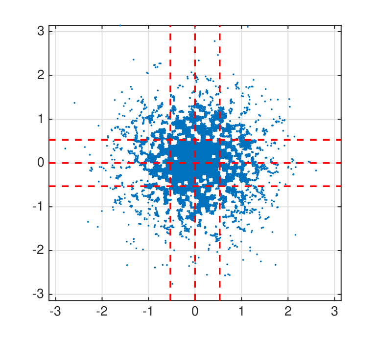
We generate the $u$–$v$ coverage randomly through Gaussian sampling, with $0$ mean and variance of $0.25$ of the maximum frequency. To simulate the incomplete sampling typically available in RI, we introduce holes predominantly in the high frequency data using an inverse Gaussian profile. We use $M=5N$ measurements, split into $d=16$ equal size blocks. An example with normalised frequencies is presented in Fig. 1. The measurement data are corrupted by complex Gaussian noise with $0$ mean producing a signal to noise level of $20~\rm{dB}$. The bounds $\epsilon_{i}$, estimated based on the noise level, are set to the $0.99$ percentile of the $\chi^{2}$ distribution with $2M_{i}$ degrees of freedom, which models the residual norm. We assume no DDEs and we use $8\times 8$ interpolation kernels [8]. An oversampling ratio is $k=4$.

The parameters are $\sigma=\tfrac{1}{\|\boldsymbol{\mathrm{\Psi}}\|_{\rm{S}}^{2}}$, $\varsigma=\tfrac{1}{\|\boldsymbol{\mathrm{\Phi}}\|_{\rm{S}}^{2}}$ and $\tau=0.49$. All operator norms are computed a priori using the power method. The normalised soft-thresholding is set $\kappa=10^{-3}$. This was observed to produce the fastest convergence speed. The parameters for SDMM are as suggested by [3]. The performance is measured by the signal to noise ratio

averaged over $10$ tests with different noise realisations.

Fig. 2 contains the SNR as a function of the number of iterations for SDMM and PD-R with equal probabilities $p_{i},\forall i$. For $p_{i}=1$, when no randomisation is performed, PD-R achieves a rate of convergence similar to SDMM. Its computational cost per iteration is much lower even without any randomisation, since SDMM computes the solution to a system of equations at each iteration. If $p_{i}$ decreases, the average number of nodes needed is reduced as well, to $n=\sum_{i=1}^{d}p_{i}$. In this case, the number of iterations required for convergence increases roughly inversely proportional to $p_{i}$, reaching a proportionality factor of $2$ at the lowest probability considered. The cost per iteration for processing the data decreases proportional to the probability. Thus, if the main computational bottleneck is due to the data fidelity term and not to the computation of the Fourier transform, the overall computational cost for reaching convergence does not increase significantly. Here, the increase is up to a factor of $2$ for the lowest probabilities. The randomised updates offer greater flexibility especially when the number of computing nodes is limited.

In Fig. 3 we study the evolution of the SNR of the randomised algorithm given a limited infrastructure with $n=4$ nodes and $16$ data blocks. We enforce $\sum_{i=1}^{d}p_{i}=4$ such that on average $4$ data blocks are processed on the $4$ computing nodes available. We compare the adaptive nonuniform probability choice proposed herein with uniform probabilities $p_{i}=0.25,\forall i$. We show the results for $\hat{p}=0.5$. For larger $\hat{p}$ similar results are produced with a slight decrease in convergence speed when $\hat{p}$ approaches $1$. Different $\check{p}$ are considered. For comparison, we also include a simulation where we update only the $4$ low frequency blocks with probabilities $p_{\mathcal{L}}=1$ and ignore the high frequency ones by setting their probabilities $p_{\mathcal{H}}=0$. This shows how much the performance degrades if the high frequency data is discarded and motivates the use of randomisation. A test with no randomisation showcases the fastest achievable convergence speed. This comes at the cost of requiring $16$ data processing nodes. The proposed adaptive choice for the probabilities substantially increases the rate of convergence. For convergence it requires only half of the number of iterations needed by the uniform probability test with $p_{i}=0.25$. This essentially stabilises the overall total computational cost required for convergence making it roughly the same to that of the algorithm performing no randomisation. It also lowers the variability of the convergence speed. Looking at it from a slightly different perspective, the full convergence curve for $\check{p}=0.05$ appears similar to that produced for a uniform probability $p_{i}=0.4$, the latter requiring on average $n=6.4$ data nodes, a $60\%$ increase, to process the data in a similar time. Finally, in Fig. 1 we also showcase the reconstructed quality of PD-R with $\sum_{i=1}^{d}p_{i}=4$, $\check{p}=0.05$ and $\hat{p}=0.5$. The quality is very similar to that achieved by the other tests for PD-R and SDMM.

We studied a distributed solver for RI imaging that uses randomised updates over the measurement blocks and we proposed a new adaptive strategy for choosing the randomisation probabilities. The algorithmic structure is highly parallelisable and has a lower computational burden if compared to existing solvers such as SDMM. The algorithm requires little configuration and produces consistently stable results. The adaptive choice of probabilities is based on the relative approximation error for each data block and is shown to accelerate the convergence speed. The approach also reduces the variability in the rate of convergence compared to the uniform randomisation. Our experiments suggest great scalability which is fundamental for the processing of data from next generation telescopes.

References

- [1] A. R. Thompson, J. M. Moran, and G. W. Swenson, Interferometry and Synthesis in Radio Astronomy. Wiley-Interscience, New York, 2001.
- [2] P. Dewdney, P. Hall, R. T. Schilizzi, and T. J. L. W. Lazio, “The Square Kilometre Array,” Proc. IEEE, vol. 97, no. 8, pp. 1482–1496, 2009.
- [3] R. E. Carrillo, J. D. McEwen, and Y. Wiaux, “PURIFY: a new approach to radio-interferometric imaging,” MNRAS, vol. 439, no. 4, pp. 3591–3604, 2014.
- [4] P. L. Combettes and J.-C. Pesquet, Fixed-Point Algorithms for Inverse Problems in Science and Engineering. Springer, New York, 2011, pp. 185–212.
- [5] N. Komodakis and J.-C. Pesquet, “Playing with duality: An overview of recent primal-dual approaches for solving large-scale optimization problems,” Signal Processing Magazine, IEEE, vol. 32, no. 6, pp. 31–54, Nov 2015.
- [6] R. E. Carrillo, J. D. McEwen, and Y. Wiaux, “Sparsity averaging reweighted analysis (SARA): a novel algorithm for radio-interferometric imaging,” MNRAS, vol. 426, no. 2, pp. 1223–1234, 2012.
- [7] A. Onose, R. E. Carrillo, A. Repetti, J. D. McEwen, J.-P. Thiran, J.-C. Pesquet, and Y. Wiaux, “Scalable splitting algorithms for big-data interferometric imaging in the SKA era,” ArXiv e-prints, Jan. 2016.
- [8] J. Fessler and B. Sutton, “Nonuniform fast Fourier transforms using min-max interpolation,” IEEE Tran. Sig. Proc., vol. 51, no. 2, pp. 560–574, Feb 2003.
- [9] S. Mallat and Z. Zhang, “Matching pursuits with time frequency dictionaries,” IEEE Trans. Sig. Proc., vol. 41, no. 12, pp. 3397–3415, Dec. 1993.
- [10] Y. Wiaux, L. Jacques, G. Puy, A. M. M. Scaife, and P. Vandergheynst, “Compressed sensing imaging techniques for radio interferometry,” MNRAS, vol. 395, no. 3, pp. 1733–1742, 2009.
- [11] J. D. McEwen and Y. Wiaux, “Compressed sensing for wide-field radio interferometric imaging,” MNRAS, vol. 413, no. 2, pp. 1318–1332, 2011.
- [12] J.-C. Pesquet and A. Repetti, “A class of randomized primal-dual algorithms for distributed optimization,” J. Nonlinear Convex Anal., vol. 16, no. 12, 2015.
- [13] L. Wolz, J. D. McEwen, F. B. Abdalla, R. E. Carrillo, and Y. Wiaux, “Revisiting the spread spectrum effect in radio interferometric imaging: a sparse variant of the w-projection algorithm,” MNRAS, vol. 463, no. 3, pp. 1993–2003, 2013.