Joint Target Detection and Tracking in Multipath Environment: A Variational Bayesian Approach
Abstract
We consider multitarget detection and tracking problem for a class of multipath detection system where one target may generate multiple measurements via multiple propagation paths, and the association relationship among targets, measurements and propagation paths is unknown. In order to effectively utilize multipath measurements from one target to improve detection and tracking performance, a tracker has to handle high-dimensional estimation of latent variables including target active/dormant meta-state, target kinematic state, and multipath data association. Based on variational Bayesian inference, we propose a novel joint detection and tracking algorithm that incorporates multipath data association, target detection and target state estimation in a unified Bayesian framework. The posterior probabilities of these latent variables are derived in a closed-form iterative manner, which is effective for reducing the performance deterioration caused by the coupling between estimation errors and identification errors. Loopy belief propagation is exploited to approximately calculate the probability of multipath data association, saving the computational cost significantly. Simulation results of over-the-horizon radar multitarget tracking show that the proposed algorithm outperforms multihypothesis multipath track fusion and multi-detection (hypothesis-oriented) multiple hypothesis tracker, especially under low signal-to-noise ratio circumstance.
Index Terms:
Joint detection and tracking, multipath data association, variational Bayesian, belief propagationI Introduction
Multitarget detection and tracking (MDT) is essential for many applications in the areas of defense, medical science, traffic control and navigation [1]. Most algorithms [2, 3] in the literature addressing MDT are based on the assumption that, in a single scan, a target generates at most one measurement and one measurement comes from at most one target. For certain sensing systems, however, one target may result in multiple measurements that are not spatially structured due to multipath propagation phenomenon [4]. Such sensing systems, called multipath detection systems (MDS) in this paper, include skywave over-the-horizon radar (OTHR) [5], passive coherent location (PCL) system [6], the sensors work in urban environments [7, 8], etc. In OTHR, high-frequency radiowave propagation through a layered ionosphere often gives rise to multiple propagation paths, resulting in multiple resolved detections for one target at each radar scan. Likewise, a PCL with multistatic configurations may also receive multiple detections from various transmitters of opportunity for a single target. Multiple delayed returns for one target may be obtained when sensors work in urban environments because of dense terrains.
For MDS, if an MDT algorithm extracts target information in multiple measurements properly, both estimation and detection performance can be improved by the increase of signal-to-noise ratio (SNR) [9]. However, as elucidated in the following, unknown measurement-to-path association brings several additional issues, making MDT for MDS more challenging. In terms of target tracking, (1) measurements need to be associated with tracked targets, and besides that a target-originated measurement needs to be associated with one of the propagation paths; (2) a tracker has to handle high-dimensional estimation of latent variables including target active/dormant meta-state, target kinematic state, and multipath data association; (3) exact computation of multipath data association is intractable due to the “combinatorial explosion” in summing out target-to-measurement-to-path association events. With regard to target detection, (1) the number of targets is unknown and time-varying, and apart from that targets may appear and disappear anytime anywhere in the absence of prior information; (2) as many as tracks from propagation paths can be produced for one target. Additionally, target detection and target tracking are tightly coupled. Existing work on MDT for MDS can be summarized as the following three categories.
Formulating MDT as two separate and sequential sub-problems, single-path target tracking [10] and multipath track fusion [11], algorithms in the first category have a simple structure and are computationally efficient. However, since only measurements from a single path are used in the single-path target tracking procedure, (multipath) tracks generated under each path are not accurate or even missed under extreme low SNR circumstance, making fused tracks unreliable.
The second category algorithms address MDT by extending single-path data association to multipath data association, such as multipath probabilistic data association (MPDA) [12, 13], multihypothesis Viterbi data association (MVDA) [14], multi-detection joint probabilistic data association (MD-JPDA) [15], multi-detection multiple hypothesis tracker (MD-MHT) [16], multi-detection probability hypothesis density (MD-PHD) [9], and multi-detection Bernoulli (MD-Bernoulli) [17]. By performing triple target-to-measurement-to-path association, these algorithms fuse information on one target at the measurement level, leading to remarkable improvement on tracking performance comparing with the first category algorithms. One drawback of the second category algorithms is that they are unable to deal with the coupling between data association and target state estimation, which means errors (e.g., a track is by chance associated with clutter or/and a measurement is associated with a wrong path) cannot be corrected once they have been made [18]. Among the above-mentioned algorithms, MPDA, MVDA and MD-Bernoulli are capable only to track a single target, while MD-JPDA assumes the number of targets is known and fixed. Others including MD-MHT and MD-PHD are able to perform MDT jointly. MD-MHT approximates the triple target-to-measurement-to-path association by path-dependent two-dimensional assignments and suffers from high computational cost. Based on the random finite set theory, MD-PHD is time-consuming as well [9].
The key idea in the third category algorithms is to perform target state estimation and data association jointly based on expectation-maximization (EM) framework [19]. The EM-based algorithms in [20, 21, 22] alternate between computing the expected complete log-likelihood according to the posterior probability density function (PDF) of missing data (multipath data association) in E-Step and optimizing it with respect to (w.r.t.) the model parameters (state estimation) in M-Step, which are attractive and desirable to reduce the performance deterioration caused by the coupling between identification errors (from data association) and estimation errors [23]. However, these work considered a single target tracking. Extending the work of [20, 21, 22] to multitarget tracking with time-varying number of targets would give rise to high-dimensional latent variables, in which case the EM algorithm may suffer from slow convergence [24].
Unlike EM that requires to calculate the conditional expectation of high-dimensional latent variables, variational Bayes (VB) [25], as an extension of EM algorithm, casts an inference problem as an optimization problem and provides analytical approximations to the posterior distributions of latent variables, and is superior to EM for complex graphical models [26]. VB is gaining popularity within the target tracking community due to its following capabilities and advantages: (1) it provides a unified Bayesian framework for joint detection and tracking; (2) it tackles the coupling issue between estimation of latent variables via an iterative optimization; (3) it avoids the enumeration of association hypotheses by using message passing on graphical models; (4) it converges under mild conditions [26]. Based on VB, Säarkkä and Nummenmaa [27] proposed an adaptive Kalman filtering method to joint estimation of dynamic state and the time-varying parameters of measurement noise. Laet et al. [28] proposed an online two-level multitarget tracking and detection algorithm for targets with multiple measurements, where VB is used in the measurement clustering level. Lázaro-Gredilla et al. [29] introduced a mixture of Gaussian processes to model the mixed measurements received from multiple targets. The hyperparameters of the mixture Gaussian are learned based on VB. Orguner [30] proposed a VB based method for extended target tracking. Turner et al. [18] proposed a VB-based tracker integrating track management, data association, and state estimation via an iterative manner, where belief propagation is used to solve data association problem. Lau et al. [31] proposed a multitarget tracking and detection algorithm based on structured mean-field VB. Williams and Lau [32] proposed a multiple scan data association method based on convex fractional free energy. However, to our best knowledge, no one has considered MDT for MDS by using VB.
This paper considers the MDT problem for MDS, and aims to derive the joint posterior distribution over the high-dimensional latent variables including target kinematic state, target active/dormant meta-state and multipath data association given the received measurements. By leveraging on Mean-field VB, the joint posterior distribution over the high-dimensional latent variables is approximated by a distribution which is from the family of the product of individual posterior distributions over target kinematic state, target meta-state and multipath data association, and that has the minimal Kullback-Leibler (KL) divergence to the joint posterior distribution. The prior distribution functions of target kinematic state, target meta-state and multipath data association are constructed from exponential family. Coordinate ascent together with an iterative mechanism are used to optimize the approximate posterior distributions over target kinematic state, target meta-state and multipath data association. In each iteration, fixed-interval smoother, forward-backward algorithm are used to estimate target kinematic state and target meta-state, respectively. Modeled by a factor graph, multipath data association integrates measurements from multiple path at the measurement level and the corresponding association probability is approximated by loopy belief propagation (LBP). In summary, the key contributions of this paper are as follows.
- •
For the first time, we incorporate multipath data association, target detection and target kinematic state estimation in a unified Bayesian framework for joint MDT of MDS.
- •
We propose a computationally efficient joint MDT algorithm for MDS, JDT-VB, which fuses information on one target at the measurement level and is capable of minimizing the performance deterioration caused by the coupling between identification errors and estimation errors, improving target detection and tracking performance for MDS significantly.
- •
To circumvent the enumeration of all joint multipath data association hypotheses, a factor graph for modeling the multipath data association is presented, and the corresponding marginal association probability is approximated by LBP.
Our work in this paper was inspired by the work of [18] but differs from [18] in three main aspects. Firstly, multiple propagation paths are involved in measurement equation, making MDT more challenging. Secondly, a new technique is proposed for estimating target kinematic state by fusing the path-dependent state estimates. Thirdly, a new factor graph is used for modeling multipath data association.
A preliminary version of the results presented here appeared in two conference papers [33, 34]. Here, we present for the first time the entire formulation including implementation details, and also supplement initialization, computational complexity analysis and simulations of the proposed algorithm.
The rest of the paper is organized as follows. The problem formulation of joint MDT for MDS is described in Section II. The closed-form analytical solutions of target meta-state estimation, target kinematic state estimation and multipath data association are derived in Section III. The simulation analysis and the conclusion are given in Section IV and Section V, respectively.
II Problem Formulation
Consider the following discrete-time dynamic system
| (1) |
where is the th target kinematic state to be estimated at time (scan) with being the dimension of , is the known kinematic state transition function, and is a zero-mean Gaussian white noise with known covariance matrix . Here, is the maximum number of targets in the region of interest, which can be determined by counting all candidate tracks (targets) in initialization stage. The initial kinematic states of targets , are assumed to be Gaussian distributed.
Denote as the th measurement at time with being the dimension of and being the known number of measurements. For the MDS, each received measurement might be originated from an underlying target through a particular propagation path or clutter. The multipath measurement model for the MDS is as follows.
| (2) |
where , , is the measurement function of the th propagation path with being the known number of paths, and is the corresponding measurement noise, which is assumed to be a zero-mean Gaussian random variable with covariance . Here, , and are assumed to be independent. As in [1], the false measurement (clutter) is assumed to be uniformly distributed in the region of interest and the number of clutter per scan is assumed to follow a Poisson distribution.

As illustrated by Fig. 1, the target-to-measurement-to-path association event (or hypothesis) represents that the th measurement is originated from the th target via the th path. For , means that the th target is not detectable by the th path. We use to represent that the th measurement is originated from clutter since a clutter is irrespective of the propagation path. Let be a joint event.
By the assumptions that a measurement via any one propagation path has only one source, for each propagation path at most one measurement is received from a target, and a measurement of a target is received through at most one propagation path [16], the joint event is constrained by the following equation group.
| (3) |
A joint event is feasible if it satisfies equation group (3). Note that merged measurements that may be originated from multiple targets via different propagation paths are not considered in this paper.
Define the binary variable to represent the active/dormant meta-state of target . By active state of a target we mean that the target is detectable with high probability. On the contrary, a target is in dormant state if it is hardly detectable or it disappears. Here, if target is in active state at time and if target is in dormant state. The sets of measurements, target kinematic state, target meta-state are defined by , , , respectively. Note that targets may appear/disappear at different time in the region of interest, i.e., they may have different lifetime. For ease of exposition (and without loss of generality), we hereafter restrict the notation on the lifetime of all targets from to . The sequences of sets , , and refer to the collections of measurements, target kinematic state, target meta-state, target-to-measurement-to-path association events up to and including time , respectively. That is, , , , . In this paper, target state variables (e.g., , ) and data association variables (e.g., ), which are not directly observed but are rather inferred from measurements (e.g., ), are called latent variables.
Based on the models of target kinematic state, target meta-state, multipath measurement and multipath data association, our problem of joint MDT for MDS is to concurrently estimate target kinematic state (tracking) and target meta-state (detection), given measurements in the presence of unknown multipath data association , i.e.,
| (4) |
A common way to solve the above-stated joint MDT problem (Eq. (4)) is to calculate joint posterior PDF first, and then marginalize the joint posterior PDF to obtain the posterior PDF of target kinematic state and posterior probability mass function (PMF) of target meta-state . Since the number of multipath data association events increases exponentially with the number of targets, the number of (validated) measurements and the number of paths, exact calculation of is computationally expensive and approximation solutions are often sought. The sampling-based stochastic approximation methods (e.g., MCMC) are computationally intensive [25]. VB, as an analytical-based deterministic approximation method, is more computationally effective and suited to MDT problem of MDS.
III VB for Joint Detection and Tracking
VB provides a local-optimal, exact analytical solution to the approximation of an inference problem, making it more competitive in the case of high-dimensional latent variables. In this paper, we employ VB to solve the joint MDT of MDS.
The first step in applying VB is to pick up a simpler family of probability densities over the latent variables . We will specify the form of the family we use later. Then, we seek the distribution closest to the posterior PDF in this family and use it to approximate , i.e., . We choose the commonly used Kullack-Leibler (KL) divergence as the dissimilarity function of two distributions. The KL-divergence from the density to the density is defined as
| (5) |
where
| (6) |
is known as the variational free energy, which is also the lower bound for the evidence since the is nonnegative. Evidently, minimizing is equivalent to maximizing .
We use mean-field variational family [25] where is partitioned into three disjoint groups , , and each of the factors , , is a probability distribution with a free functional form. The joint distribution over high-dimensional latent variables are represented by the product of individual PDFs (or PMF) of the low-dimensional latent variable. That is,
| (7) |
In general, is non-convex and no explicit solution for can be found. Coordinate ascent, a computationally effective technique with competitive performance for large-scale non-convex machine learning problems, is exploited to maximize Eq. (6). Next we show how to apply coordinate ascent to solve Eq. (6).
Substitute Eq. (7) into Eq. (6), and rewrite Eq. (6) as a function of the factor for example, one obtains,
| (8) |
where , a constant w.r.t. . Let
| (9) |
where is the normalization constant.
Clearly, takes the maximum value when . Similarly,
| (11) |
Note that , , are not explicit solutions since calculation of any depends on expectations computed w.r.t. the other two factors. Therefore, the iterative mechanism, which starts from appropriately initialized and then cycles through the factors and update each in turn by recalculating it using the current values for the other two factors, is resorted to estimating . Since is convex w.r.t. each of the factors, the eventually derived estimation of the factors are local optimal [26].
Based on the principled application of VB described above, we next propose a joint MDT algorithm named JDT-VB for MDS. In the following, we first present the framework of the proposed JDT-VB algorithm, and then provide all the implementation details.
III-A Framework of JDT-VB Algorithm
In the same vein of [18], the interdependence among the variables in the joint MDT problem can be described by the graphical model shown in Fig. 2. Target kinematic state and target meta-state evolve with first-order Markov process. Multipath data association is assumed to be independent over time. At each time, observable variable is generated from via a particular path or clutter, and the relationship among target-to-measurement-to-path association is represented by . Additionally, is related to target meta-state . Given multipath data association , the measurements are independent from target meta-state . The joint PDFs can be factorized as
| (12) |
Based on the graphical model in Fig. 2, the framework of the proposed JDT-VB algorithm is depicted in Fig. 3. After constructing the prior probabilities of latent variables, the posterior PDFs or PMF of target kinematic state, target meta-state, and multipath data association are updated in an iterative loop. The details are further explained below.
- •
Prior PDFs modeling: one convenient and favorable class of priors is conjugate priors in the exponential family. In this paper, the prior PDFs (or PMFs) of target kinematic state, target meta-state and multipath data association are assumed to be a Gaussian distribution, a Bernoulli distribution, and a distribution in exponential family composed of a Poisson distribution and a Bernoulli distribution, respectively.
- •
Posterior multipath data association update (Module 3): given the th iterative (path-unconditional) PDF of target kinematic state and PMF of target meta-state , the PDF of multipath data association belongs to exponential family. The distribution of each multipath data association event is approximately calculated by the LBP method.
- •
Posterior target kinematic state update (Module 1): given measurements and the th iterative PDF of multipath data association , the PDF of target kinematic state updated by measurements from a single path, called path-conditional PDF, is a Gaussian distribution, of which the mean and covariance are obtained via a fixed-interval smoother. The PDF of target kinematic state updated by measurement from all paths, called path-unconditional PDF and denoted by , is a Gaussian distribution as well, and is obtained by fusing the path-conditional PDFs of target kinematic state.
- •
Posterior target meta-state update (Module 2): given the th iterative PDF of multipath data association , the PMF of target meta-state is updated via forward-backward algorithm, which is able to integrate statistical information (e.g., detection probability, false alarm rate) relevant to the specific application.
- •
Iterative loop: Module 1- Module 3 above are repeated until at two consecutive iterations are close enough or the maximum number of iterations is reached.
III-B The Conjugate Prior PDFs and Observation Modeling
III-B1 Target Kinematic State Modeling
As seen from Fig 2, each target is assumed to independently follow a first-order Markov process, that is,
| (13) |
where .
III-B2 Target meta-state Modeling
The meta-state of each target is assumed to independently follow a two-state Markov model as shown in Fig 2,
| (14) |
The initial probability and transition probabilities are assumed to be known. The detection decision on target is made based on .
III-B3 Multipath Data Association Modeling
The PDF of multipath data association consisting of a Poisson distribution to model clutter and a Bernoulli distribution to model target detection, is given by
| (15) |
where
| (16) |
is the number of measurements that are not associated with any target in the joint event , is the path-dependent detection indicator of target that indicates whether a measurement is associated with target via path in , represents the clutter density, is the detection probability of target via path , and represents the volume of the region of interest, which is the volume of the validation region when gating technique is used [1]. Note that the detection probability of target via path , , is a function of target active/dormant meta-state . That is, takes a relatively large value if target is in the active state (), and vice versa. See Appendix A for the detailed derivation of Eq. (15).
III-B4 Observation Modeling
Based on the assumption that measurements are independently distributed conditioned on target kinematic state and multipath data association events (see the graphical model in Fig. 2), the likelihood function can be factorized as
| (17) |
Recall that is a joint feasible data association event. If , , that is, no target exists, then measurement is from clutter and
| (18) |
by the assumption that the clutter is uniformly distributed in the region of interest [1]. If , , that is, target is not detected via path , then
| (19) |
Otherwise, if , , , that is, measurement is originated from target through propagation path , we have
| (20) |
By Eqs. (18), (19), (20) and expanding the right side of Eq. (17), likelihood function (17) is rewritten as
| (21) |
Note that observation likelihood represents the likelihood of the measurements for the given target states and a joint feasible data association event that is an assignment among measurements, targets and propagation paths. The clutter density is not involved in .
III-C Posterior Probability Update of JDT-VB
Based on the conditional independence of approximate distributions imposed by mean-field method, the approximate posteriors on target kinematic state and target meta-state are factorized over tracks, and approximate posteriors on multipath data association is factorized over time, that is,
| (22) | |||
| (23) |
III-C1 Calculation of
According to the definition of Eq. (9) and the factorization in Eq. (22), the update of posterior PDF of each track can be derived separately as follows.
| (24) |
In the vein of Eq. (12), the PDF is decomposed as
| (25) |
Substituting Eq. (25) into Eq. (24), and by
yield
| (26) |
where is independent with . By a similar derivation of Eq. (21), the expectation is expanded as
| (27) |
where is independent with .
Substituting Eq. (27) into Eq. (26), taking the exponential of both sides of Eq. (26), and throwing away the terms ( and ) that do not depend on , yield
| (28) |
By applying the product of Gaussian PDFs (see details in Appendix B), we obtain
| (29) |
where
| (30) |
are synthetic measurement and its corresponding measurement covariance. Substituting Eq. (29) into Eq. (28), yields,
| (31) |
From Eq. (31), it is seen that is equivalent to a dynamical system with multiple (independent) synthetic measurements and corresponding measurement covariance . Note that since for different propagation path , the measurement functions are different, the synthetic measurements cannot be synthesized further over all paths. Here, we approximate Eq. (31) by fusing path-dependent kinematic state PDFs which are obtained by Kalman smoother for linear system and URTS for nonlinear system [35] based on the synthetic measurements corresponding to the path, that is,
| (32) |
where , are the mean and covariance of path-dependent kinematic state PDFs. In Eq. (32), the interdependency of the path-dependent kinematic state PDFs are neglected.
In order to reduce computational cost, gating technique [1] can be applied to eliminate very unlikely association between targets and measurements. Accordingly, the candidate measurements for posterior PDF update of target under path should fall into the relevant validation region, which is defined as follows [1]:
| (33) |
In Eq. (33), for current iteration , measurement prediction and the associated innovation covariance , where , are the estimated target kinematic state and the corresponding covariance in the last iteration , respectively. is the Jacobian matrix of w.r.t. . represents Mahalanobis distance. The constant is chosen to make gate probability equal to . The volume of the validation region is [1]
| (34) |
where the coefficient depends on the measurement dimension . For , .
The validation region for multipath measurements is then defined to be the union of the multipath validation regions for all targets. Calculating the volume of the validation region for multipath measurements, required by the calculation of data association probability, is complicated since the multipath validation region for each target may overlap [12]. As in [12], here we approximate the volume by
| (35) |
Consequently, the synthetic measurement and its corresponding measurement covariance in Eq. (30) can be rewritten as
| (36) |
The calculation of for the case of linear dynamic system is summarized in Module 1.
III-C2 Calculation of
By Eq. (11), Eq. (22) and the dependence of multipath data association on target meta-state shown in Fig. 2, for each target , we have
| (37) |
Substituting Eq. (15) into Eq. (37), yields,
| (38) |
with
| (39) |
See Appendix C for the detailed derivations of Eq. (38).
Recall that represents the event that target is detected via path in the joint association event . Therefore,
| (40) |
From Eq. (38), the posterior PMF of target meta-state can be updated via a forward-backward algorithm [36]. Note that integrates the detection probability , resulting in improvement of the detection performance since information from all paths are integrated. The calculation of is summarized in Module 2.
III-C3 Calculation of
By Eq. (11) and Eq. (23), the dependence of multipath data association on target meta-state, and the dependence of measurement on target kinematic state and multipath data association shown in Fig. 2, for each time , we rewrite as
| (41) |
Reshape as a column vector . Take the exponential of both sides of Eq. (41) and rewrite it in the form of exponential family with a parameter that has the same dimension with .
| (42) |
where , and
| (43) |
In Eq. (42), the constant is the Poisson distribution with mean , and is the set of feasible joint multipath data association events. See Appendix D for the detailed derivations of Eqs. (42)-(43).
Calculating the exact expectation from Eq. (42) requires the enumeration of all feasible target-to-measurement-to-path events, which is intractable since the number of feasible association events increases exponentially with the increasing of the numbers of targets, measurements and paths. Recently, the belief propagation schemes for data association have attracted much attention [37, 38, 32, 39, 40]. LBP runs belief propagation on a graph containing loops. Here, by constructing the factor graph corresponding to the triple target-to-measurement-to-path association, we extend the LBP of [18] to approximate the marginal probabilities of multipath data association. Note that, as in [16], an alternative way to solve triple target-measurement-path association problem is to reduce it to a regular (non-multipath) data association problem, with each (target, path) acting as a pseudo-target. By formulating the reduced problem as a two-dimensional maximum weighted matching problem, the technique in [18, 38] can be applied immediately. However, the constraints on the triple target-measurement-path association in this paper, i.e., equation group (3) (particularly the first equation), making the reduced two-dimensional association problem not a two-dimensional maximum weighted matching problem, and therefore prohibit applying the technique in [18, 38] to the triple target-measurement-path association in this paper.
By expending the joint association event , the posterior PDF can be represented as a factor graph
| (44) |
with
being factors, and being variables.
Fig. 4 provides an exemplified factor graph [41] for modeling the association event in Fig. 1. There are four kinds of factors in factor graph, row factor , column factor , page factor , and evidence factor . We define the follow messages for LBP (omit subscript for simplicity):
where denotes the message sent from factor to variable with being the state of , and denotes the message sent from variable to factor . Using the standard update rules of BP [42], a message from a variable to a factor is
| (45) |
and a message from a factor to a variable is
| (46) |
where is the set of neighboring factors to variable , and is the set of neighboring variables to factor .
Message computation consists of message initialization step and message update step. The evidence factor (leaf factor node) is utilized to initialize messages via Eq. (47), and the rest factors are used to update messages. Due to the fact that there is only one nonzero value in any row/column/page of , the messages , , and are given as Eqs. (48)-(50), respectively.
| (47) | |||
| (48) | |||
| (49) | |||
| (50) |
By the fact that each variable connects to factors , and , the messages from variable to factor , and () are given as
| (51) | |||
| (52) | |||
| (53) |
For or , the factors and only connect to the factor , that is, , .
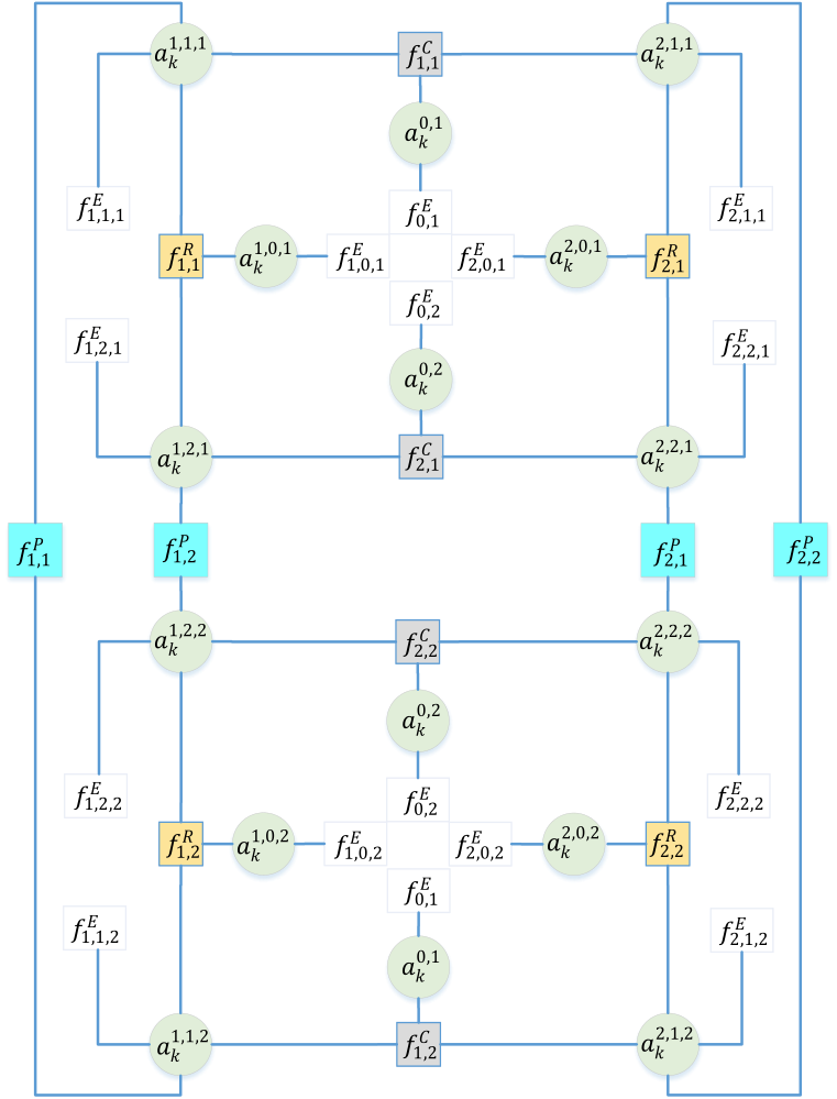
The messages are updated iteratively according to the factor graph. Once the iteration process terminates, the estimated marginal distribution of each variable with its expectation can be computed by multiplying the corresponding messages from adjoining factors corresponding to the variable, that is,
| (54) | |||
| (55) |
See Appendix E for the detailed derivation of LBP for multipath data association.
The computation of is summarized in Module 3.
Remark 1: In [38], Williams and Lau considered the LBP for the two-way data association problem, i.e., the correspondence between targets and measurements, in a single frame. By modeling the two-way data association problem as a maximum weighted matching problem on a bipartite graph and showing that the message update equations are contractions, the LBP was proved to converge [38]. However, the technique in [38] may not be applied to the triple target-measurement-path association that is a three-matching problem in this paper. So the convergence of the LBP in the present paper is not guaranteed a priori. In the Supplement Material (Appendix A), we provide a toy example (two targets, four propagation paths, low clutter rate) to observe the convergence of the LBP algorithm. Divergence of the LBP is not seen in extensive simulations of the toy example. It is our future work to investigate the convergence property of the LBP for the triple target-measurement-path association.
Remark 2: By Eq. (44), the factor graph that models the multipath data association with targets, measurements and paths has variables , factors (consisting of constraint factors , and , and evidence factor node ). By the fact that each variable connects with four factors (, , and ), each connects with two factors ( and ), and each connects with two factors ( and ), there are total edges in the factor graph. For applications with a large number of targets and measurements, the gating technique can exclude the very unlikely target-to-measurement associations, reducing the number of variables and constraint factors of the factor graph.
III-D The JDT-VB Algorithm and Its Computational Complexity
The JDT-VB algorithm consisting of Modules 1, 2 and 3 is summarized in TABLE. I. The iteration terminates if between two consecutive iterations are close enough or the maximum number of iterations is reached.
| ||
|---|---|---|
| ||
| (2.2) Detection: Estimate via Module 2. | ||
| (2.3) Tracking: Estimate via Module 1. | ||
| ||
|
The computational complexity of JDT-VB is equal to the sum of the computational cost of Modules 1, 2 and 3, i.e.,
| (56) |
where is the number of JDT-VB iterations, and , , are the computational complexity of Modules 1, 2 and 3, respectively. For Module 1, [35] which is proportional to the sum of computational cost of path-dependent state estimation and multipath state fusion. Module 2 is carried out by forward and backward algorithm, and its computational complexity [36]. The LBP algorithm is used to approximate the multipath data association in Module 3. The main cost of LBP is the message update equation, which is for each variable at each iterations [43] with being the number of possible values of variable . In our graphical model, there are total variables, and each variable takes values of 0 and 1, i.e., . Hence, the computational cost with being the number of LBP iterations. At each iteration, the computational cost of JDT-VB increases linearly with the number of targets, measurements and propagation paths.
Remark 3: There are several properties of JDT-VB:
- •
it provides an integrated solution for joint MDT for MDS in VB framework. The performance of detection and tracking is improved by the fact that multipath measurements are integrated to estimate target kinematic state and target meta-state.
- •
it has a closed-loop iterative manner among multipath data association, kinematic state estimation, and meta-state estimation, which is effective in dealing with the coupling relationship between estimation errors and identification errors in the view of feedback control.
- •
it has polynomial computational complexity. The multipath data association is modeled by a probabilistic graphical model, and the marginal association probabilities are calculated approximately by the LBP algorithm.
III-E Initialization of JDT-VB
- •
In scan , we coarsely group the measurements that have not been used to update existing tracks into different subsets , . In each subset , any two measurements are within a preset threshold vector conditioned on the assumption that they are from the same target. Subsets with at least two measurements are utilized to initialize heads of new tracks by the assumption that it is rare to receive the measurement only from one path for a target under the circumstance of multipath propagation. Considering each subset with at least two measurements, for each measurement-to-path association hypothesis, we transform the measurements in from measurement space to kinematic state space, obtaining a set of the transformed kinematic states. The kinematic state estimate is obtained by fusing the transformed kinematic states which have the minimum average Mahalanobis distance. The covariance is pre-determined based on measurement noise covariance. Set the initial probability .
- •
In scan , target kinematic state estimation and is performed individually by using LBP and UKF. Meanwhile, the probability is recursively updated by using the forward-backward algorithm according to the Module 2. If the average detection probability of target in three successive scans is less than the threshold , the track is deleted. The measurements that do not fall into validation gates of any tracks are used to initialize new tracks. is the total number of confirmed temporary tracks at scan .
IV Simulation
OTHR exploits the reflection effect of the ionosphere for high-frequency signal (3-30MHz) to detect and track airborne/surface targets at ranges an order of magnitude greater than conventional line-of-sight radars [5]. As mentioned in Section I, multipath propagation phenomenon often appears in OTHR [12] due to the multilayer structure of the ionosphere, resulting in multiple measurements from one target. The correspondence among targets, measurements and propagation paths is unknown.
The performance of JDT-VB is evaluated and compared against MPTF [11] and multi-detection multiple hypothesis tracker using the OTHR target tracking scenario. For MPTF, multiple path-dependent tracks are obtained in slant coordinate by using PDA and UKF. Then, these path-dependent tracks are fused to derive target kinematic states in the ground coordinate. As a multi-scan joint detection and tracking algorithm for MDS, MD-MHT [16] approximates the three-dimensional multipath data association by path-dependent two-dimensional assignments and is a suboptimal but computational effective MHT algorithm. In [16], MD-MHT is carried out based on the track-oriented framework and solved by multiple frame assignment algorithm. We here use the hypothesis-oriented framework together with Murty’s approximation method [44, 45], which is called MD-HMHT. MD-PHD [9], which is limited to track a few high-value targets due to its high computational cost [9], is not considered here.
IV-A Multitarget Tracking in OTHR Scenario
We consider an ionospheric model with two layers, E-layer and F-layer. There are four paths in total, i.e., EE path, EF path, FE path and FF path. Refer to TABLE. II for the corresponding look-up path table.
| Index | Path | Explanation | |||
|---|---|---|---|---|---|
| EE | transmit on E and receive on E | ||||
| EF | transmit on E and receive on F | ||||
| FE | transmit on F and receive on E | ||||
| FF | transmit on F and receive on F |
The OTHR measurement in slant coordinates consists of slant range , slant range rate and azimuth . The target kinematic state in ground coordinates consists of ground range , ground range rate , bearing and bearing rate . The measurement function is given by [12]
| (57) |
with
where and are the ray path of transmitter and receiver, and is the distance between the receiver and the transmitter.
IV-A1 Scenario parameters
The surveillance region is assumed to be km in range, rad in azimuth, and km/s in range rate. Four targets move in the surveillance region with near-constant velocity (see Fig. 5a). Two of them (Target 1 and Target 2) move in parallel. The other two (Target 3 and Target 4) cross at . Initial kinematic states and lifetime of the targets are given in TABLE. III. The sampling period s, and the number of scans . The standard deviation of the slant range, Doppler and azimuth measurement errors for all paths are km, km/s, and rad, respectively. The power spectral density of the process noise for targets is set to km2/s3 in both -direction and -direction. For ionosphere, , km and km. The distance between the transmitter and the receiver km.
| Target | Initial state | Lifetime |
|---|---|---|
| [1, 20] | ||
| [1, 20] | ||
| [10, 30] | ||
| [10, 30] |
The performance of detection and tracking algorithms is related to the number of clutter and the detection probability . Without loss of generality, we do not distinguish the detection probabilities of different paths, i.e., for . We compare the performance of JDT-VB, MPTF and MD-HMHT by varying the values of and . 100 Monte Carlo runs are carried out. All the three algorithms are implemented in MATLAB on a PC with an Intel CORE i5 CPU and 4GB RAM.
IV-A2 Algorithm parameters
For JDT-VB, the threshold for the convergence of and the maximum number of iterations for JDT-VB . Thresholds for the initialization of track heads . The threshold for track confirmation . The initial target meta-state probability is given by the initialization, and transition probabilities for target meta-state are and . For MPTF, M/N logic rule with parameter 2/2 & 1/3 is used for track confirmation. For MD-HMHT, the Murty’s approximation method keeps the first best hypothesis (in this paper, when and when ). The window length of MD-HMHT is set to be three. For both MPTF and MD-HMHT, a track will be deleted if no measurement falls into the gate of the track over three successive scans when or five successive scans when . The gate probability for all of the algorithms.
IV-B Performance Evaluation
IV-B1 Performance Metrics Calculation
The following performance metrics are used to evaluate the tracking algorithms.
- •
Number of Valid Tracks (NVT )
- •
Track Probability of Detection (TPD )
- •
Number of False Tracks (NFT )
- •
Tentative Track Latency (TTL )
- •
Average Euclidean Error (AEE )
- •
Mean Optimal Subpattern Assignment (MOSPA ) [46]
- •
Total Execution Time (TET )
For the definitions of NVT, TPD, NFT, TTL, AEE, TET, the reader can refer to [47]. Values of the metrics are computed by averaging over all Monte Carlo runs. () indicates the higher (lower) value the metric, the better (worse) the performance is. Note that tracks with minimum length five are used to calculate the metrics.
IV-B2 Performance comparison
Fig. 5b shows the multipath detections of the four targets and clutter over all scans when . The trajectories obtained by MPTF and JDT-VB in a single run () are shown in Fig. 6. From Fig. 6a, it is seen that MPTF successfully tracks all four targets. However, one false track (Trk-5) from clutter and one ghost track (Trk-6) caused by the unsuccessful fusion of multipath tracks corresponding to Target 4 appear as well. Fig. 6b shows that MD-HMHT successfully tracks all four targets without producing false track or ghost track. Comparatively, as shown in Fig. 6c, the tracks for the four targets obtained by JDT-VB are more smoother and no false track or ghost track is generated.
| SNR |
|
|
|
| ||||||||||||
|---|---|---|---|---|---|---|---|---|---|---|---|---|---|---|---|---|
| Metrics | MPTF | MD-HMHT | JDT-VB | MPTF | MD-HMHT | JDT-VB | MPTF | MD-HMHT | JDT-VB | MPTF | MD-HMHT | JDT-VB | ||||
| NVT | 3.92 | 3.88 | 3.80 | 3.84 | 3.31 | 3.72 | 2.04 | 3.04 | 3.50 | 1.88 | 1.91 | 3.23 | ||||
| TPD | 0.99 | 0.96 | 0.97 | 0.99 | 0.86 | 0.96 | 0.63 | 0.63 | 0.88 | 0.65 | 0.45 | 0.87 | ||||
| NFT | 1.86 | 0.40 | 0.57 | 12.7 | 1.21 | 2.18 | 3.93 | 0.51 | 0.94 | 15.2 | 1.14 | 1.90 | ||||
| TTL | 0.24 | 0.47 | 0.38 | 0.14 | 0.69 | 0.70 | 3.44 | 0.14 | 0.38 | 3.58 | 0.70 | 0.48 | ||||
| AEE-R1 | 1.56 | 2.47 | 1.59 | 1.6 | 3.01 | 1.88 | 2.49 | 4.03 | 2.19 | 2.47 | 4.33 | 2.41 | ||||
| AEE-B1 | 1.42 | 1.20 | 0.58 | 1.54 | 1.80 | 0.50 | 2.28 | 2.10 | 0.98 | 2.24 | 2.30 | 1.16 | ||||
| MOSPA | 18.7 | 10.9 | 10.4 | 37.5 | 31.6 | 22.4 | 30.8 | 31.2 | 18.2 | 39.6 | 39.7 | 23.1 | ||||
| TET (s) | 9.08 | 81.8 | 7.42 | 58.6 | 1279 | 79.6 | 22.4 | 76.1 | 7.85 | 48.5 | 1233 | 82.4 | ||||
- 1
AEE-R (km) and AEE-B (mrad) are the AEE in the direction of ground range and bearing, respectively.
TABLE IV provides the statistical performance of MPTF, MD-HMHT and JDT-VB when takes values and takes values . As expected, the higher the SNR (higher detection probability and less number of clutter), the better their performance is. Specifically, in terms of NVT and TPD, JDT-VB performs better and better than MPTF and MD-HMHT with the decreasing of although their performances are comparable in the case of . This is because JDT-VB integrates the target information from multiple propagation paths at measurement level which is more beneficial to track detection, especially in the case of low detection probability (e.g., ). In the aspect of NFT, which is summation of the number of false tracks and the number of ghost tracks, the performances of JDT-VB and MD-HMHT are comparable, and are better than that of MPTF, especially when there is a large number of clutter (e.g., ). The main reason that both MD-HMHT and JDT-VB do not generate many false tracks is the adoption of the multiple measurements clustering. On TTL, JDT-VB and MD-HMHT have comparable performance, which are worse than MPTF if since it is not hard for MPTF to initialize tracks in the high detection probability case while ignoring single element subsets in the above-mentioned track initialization method for JDT-VB may generate delay for new tracks. In the low detection probability case, with the same reason as the superiority to MPTF on NVT and TPD, JDT-VB performs better. On the tracking error, JDT-VB and MPTF have comparable performance on range; however, the former performs much better than the latter on azimuth. MD-HMHT has the largest tracking error. The reason is that the marginal performance improvement brought by the iteration mechanism and state smooth of JDT-VB is decreasing (Range rate is measurable but azimuth rate is not in OTHR). The MOSPA shows that, on the whole, JDT-VB is superior to MPTF and MD-HMHT. JDT-VB runs faster than MPTF when but slower when . This is because the most computational expenditure of JDT-VB is caused by the multipath measurement clustering for track initialization; this expenditure grows fast with the increase of the number of measurements. When , the running time of track initialization takes 61.1% of the total running time of JDT-VB, which increases up to 94.4% when . MD-HMHT is most time-consuming, especially in the case of high false-alarm (e.g., ). As a whole, JDT-VB outperforms MPTF and MD-HMHT for MDT of MDS, especially under low SNR circumstance.
IV-B3 Performance analysis w.r.t. different iterations
Fig. 7 shows the performance of JDT-VB w.r.t. the number of iterations considering different and for 100 Monte Carlo runs. It is seen that JDT-VB converges quickly and its performance improves as the increasing of the number of iterations. Before the iteration starts (), the initial kinematic state error acquired by the multipath measurement clustering is large because of clutter and non-zero missed detection probability. This large state error may increase the risk of incorrect target-to-measurement-to-path association in the subsequent scans which in turn leads to large kinematic state estimation errors and/or the reduction of the track detection probability of the target. For , based on the results from the last iteration, the estimations of target kinematic state and target meta-state are improved by the smooth mechanism, leading to the reduction of incorrect target-to-measurement-to-path association which in turn improves the estimation of target kinematic state and target meta-state. By this procedure of iteration, the target detection and track performance of JDT-VB is improved significantly at the end. More simulation results including detection and tracking for each target are given in Supplementary Material.
V Conclusion
We studied the MDT problem for MDS. Based on VB, we proposed a joint detection and tracking algorithm, JDT-VB, which is a closed-loop solution among multipath data association, target kinematic state estimation, and target detection. The corresponding analytical solutions are calculated iteratively via LBP, URTS, and forward-backward algorithm, respectively. Simulations of an OTHR multitarget tracking application have shown that JDT-VB improves the performance of target detection and tracking significantly comparing with MPTF and MD-HMHT, and hence should be considered as an alternative priority for MDT of MDS. The proposed JDT-VB algorithm was implemented off-line although it is possible to develop an online version of the algorithm by replacing the fixed-interval smoother and with filters.
Appendix
V-A Derivation of
Define variables , , as detection indicators of target, measurement, and path in the joint association event , respectively. In particular, means that the th target is associated with the th measurement via propagation path . Denote the number of unassociated measurements in event . For a given , the vectors , and are completely defined. Therefore,
| (58) |
The first term in Eq. (58) is obtained from the following reasoning based on combinatorics:
- •
In event , there are target-originated measurements and false measurements.
- •
The number of joint association events in which the same set of the target-originated measurements is detected is given by the number of permutations of the measurements taken as .
Therefore, assuming that each such event is a priori equally likely, the first term in Eq. (58) is
| (59) |
Assume that , and are independent. The last term in Eq. (58) is,
| (60) |
where the PMF of the number of false measurements is
| (61) |
V-B Derivation of Eq. (29)
Rewrite the Gaussian PDF as the following canonical form
| (62) |
where , , and .
Denote and , the product of Gaussian PDFs is rewritten as
| (63) |
with .
V-C Derivation of
By the definition of Eq. (11) and the reduced factorization in Eq. (22), the updates of posterior PDF of each target’s meta-state can be derived separately as follows.
| (64) |
Substituting Eq. (25) into Eq. (64), and by
yields
| (65) |
where is independent from .
For two functions and , define if , where is an additive constant. By expanding over time and throwing away the independent terms , we have
| (66) |
Next we calculate .
Similar to Eq. (15), the conditional PDF is
| (67) |
where the detection probability is now a function of .
V-D Derivation of
By Eq. (11) and Eq. (22), the updates of posterior PDF of data association can be derived separately as follows.
| (69) |
Since
and the first two terms of Eq. (69) are independent from , we have
| (70) |
Substituting the likelihood function Eq. (21) into Eq. (70), yields Eq. (41).
In the vein of Eq. (67), the PDF is
| (71) |
Substituting Eqs. (16) and (40) into Eq. (71), and taking the logarithm of both sides of Eq. (71), yield
| (72) |
In the vein of Eq. (21), is
| (74) |
Substituting Eqs. (73) and (74) into Eq. (70), and taking the exponential of both sides of Eq. (70), yield,
| (75) |
The variational parameter are updated as follows.
- •
For , ,
- •
For , ,
- •
For , ,
(76)
with
| (77) |
Let with being the state estimation error. Assume that , i.e., is an unbiased estimation of . Let , where is the Jacobian matrix of the function . Eq. (77) is then expanded as
| (78) |
V-E LBP Derivation for Multipath Data Association
According to the standard update rules of Eq. (46), we have the message as
| (79) |
Recall that there is only one nonzero value in any row of , i.e., if , then , . Eq. (79) can be rewritten as
| (80) |
Since each variable connects to the factors , , and , the message in Eq. (80) is given by
| (81) |
Define the ratio as
| (82) |
with
| (83) |
We symmetrically apply Eqs. (80)-(83) to obtain the messages , , , and , , , as follows.
| (84) | |||
| (85) |
and
| (86) | |||
| (87) |
Finally, the marginal distribution of multipath data association is computed by normalizing the product of the incoming messages to each variable, i.e.,
| (88) |
with
| (89) |
References
- [1] Y. Bar-Shalom, X. Li, and T. Kirubarajan, Estimation with applications to tracking and navigation: theory algorithms and software. John Wiley & Sons, 2004.
- [2] I. J. Cox, “A review of statistical data association techniques for motion correspondence,” International Journal of Computer Vision, vol. 10, no. 1, pp. 53–66, 1993.
- [3] G. Pulford, “Taxonomy of multiple target tracking methods,” IEE Proceedings-Radar, Sonar and Navigation, vol. 152, no. 5, pp. 291–304, 2005.
- [4] K. Granström, M. Baum, and R. Stephan, “Extended object tracking: Introduction, overview and applications,” Journal of Advances in Information Fusion, vol. 12, pp. 1–18, 2016.
- [5] G. Fabrizio, High frequency over-the-horizon radar: fundamental principles, signal processing, and practical applications. McGraw Hill Professional, 2013.
- [6] R. Tharmarasa, M. Subramaniam, N. Nadarajah, T. Kirubarajan, and M. McDonald, “Multitarget passive coherent location with transmitter-origin and target-altitude uncertainties,” IEEE Transactions on Aerospace and Electronic Systems, vol. 48, no. 3, pp. 2530–2550, 2012.
- [7] M. Zhou, J. J. Zhang, and A. Papandreou-Suppappola, “Multiple target tracking in urban environments.” IEEE Transactions on Signal Processing, vol. 64, no. 5, pp. 1270–1279, 2016.
- [8] L. Li and J. L. Krolik, “Simultaneous target and multipath positioning,” IEEE Journal of Selected Topics in Signal Processing, vol. 8, no. 1, pp. 153–165, 2014.
- [9] X. Tang, X. Chen, M. McDonald, R. Mahler, R. Tharmarasa, and T. Kirubarajan, “A multiple-detection probability hypothesis density filter,” IEEE Transactions on Signal Processing, vol. 63, no. 8, pp. 2007–2019, 2015.
- [10] G. W. Pulford and R. J. Evans, “Probabilistic data association for systems with multiple simultaneous measurements,” Automatica, vol. 32, no. 9, pp. 1311–1316, 1996.
- [11] D. J. Percival and K. A. White, “Multihypothesis fusion of multipath over-the-horizon radar tracks,” in Proceedings of SPIE, vol. 3373, 1998, pp. 440–451.
- [12] G. W. Pulford and R. J. Evans, “A multipath data association tracker for over-the-horizon radar,” IEEE Transactions on Aerospace and Electronic Systems, vol. 34, no. 4, pp. 1165–1183, 1998.
- [13] G. Pulford, “OTHR multipath tracking with uncertain coordinate registration,” IEEE Transactions on Aerospace and Electronic Systems, vol. 40, no. 1, pp. 38–56, 2004.
- [14] G. Pulford and B. La Scala, “Multihypothesis Viterbi data association: Algorithm development and assessment,” IEEE Transactions on Aerospace and Electronic Systems, vol. 46, no. 2, pp. 583–609, 2010.
- [15] B. Habtemariam, R. Tharmarasa, T. Thayaparan, M. Mallick, and T. Kirubarajan, “A multiple-detection joint probabilistic data association filter,” IEEE Journal of Selected Topics in Signal Processing, vol. 7, no. 3, pp. 461 – 471, 2013.
- [16] T. Sathyan, T.-J. Chin, S. Arulampalam, and D. Suter, “A multiple hypothesis tracker for multitarget tracking with multiple simultaneous measurements,” IEEE Journal of Selected Topics in Signal Processing, vol. 7, no. 3, pp. 448 – 460, 2013.
- [17] J. Chen, H. Ma, C. Liang, and Y. Zhang, “OTHR multipath tracking using the Bernoulli filter,” IEEE Transactions on Aerospace and Electronic Systems, vol. 50, no. 3, pp. 1974–1990, 2014.
- [18] R. D. Turner, S. Bottone, and B. Avasarala, “A complete variational tracker,” in Advances in Neural Information Processing Systems 27. Montreal, Canada: Curran Associates, Inc., 2014, pp. 496 – 504.
- [19] A. P. Dempster, N. M. Laird, and D. B. Rubin, “Maximum likelihood from incomplete data via the EM algorithm,” Journal of the Royal Statistical Society. Series B (Methodological), vol. 39, no. 1, pp. 1–38, 1977.
- [20] G. W. Pulford and A. Logothetis, “An expectation-maximisation tracker for multiple observations of a single target in clutter,” in Proceedings of the 36th IEEE Conference on Decision and Control, vol. 5, 1997, pp. 4997–5003.
- [21] H. Lan, Y. Liang, Q. Pan, F. Yang, and C. Guan, “An EM algorithm for multipath state estimation in OTHR target tracking.” IEEE Transactions on Signal Processing, vol. 62, no. 11, pp. 2814–2826, 2014.
- [22] H. Lan, Y. Liang, Z. Wang, F. Yang, and Q. Pan, “Distributed ECM algorithm for OTHR multipath target tracking with unknown ionospheric heights,” IEEE Journal of Selected Topics in Signal Processing, vol. 12, no. 1, pp. 61–75, 2018.
- [23] H. Lan, X. Wang, Q. Pan, F. Yang, Z. Wang, and Y. Liang, “A survey on joint tracking using expectation–maximization based techniques,” Information Fusion, vol. 30, pp. 52–68, 2016.
- [24] D. G. Tzikas, A. C. Likas, and N. P. Galatsanos, “The variational approximation for Bayesian inference,” IEEE Signal Processing Magazine, vol. 25, no. 6, pp. 131–146, 2008.
- [25] D. Blei, A. Kucukelbir, and J. McAuliffe, “Variational inference: A review for statisticians,” Journal of the American Statistical Association, vol. 112, no. 518, pp. 859 – 877, 2017.
- [26] C. M. Bishop, Pattern recognition and machine learning. springer, 2006.
- [27] S. Särkkä and A. Nummenmaa, “Recursive noise adaptive Kalman filtering by variational Bayesian approximations,” IEEE Transactions on Automatic Control, vol. 54, no. 3, pp. 596 – 600, 2009.
- [28] T. De Laet, H. Bruyninckx, and J. De Schutter, “Shape-based online multitarget tracking and detection for targets causing multiple measurements: Variational bayesian clustering and lossless data association,” IEEE Transactions on Pattern Analysis and Machine Intelligence, vol. 33, no. 12, pp. 2477–2491, 2011.
- [29] M. Lázaro-Gredilla, S. Van Vaerenbergh, and N. D. Lawrence, “Overlapping mixtures of Gaussian processes for the data association problem,” Pattern Recognition, vol. 45, no. 4, pp. 1386–1395, 2012.
- [30] U. Orguner, “A variational measurement update for extended target tracking with random matrices,” IEEE Transactions on Signal Processing, vol. 60, no. 7, pp. 3827–3834, 2012.
- [31] R. A. Lau and J. L. Williams, “A structured mean field approach for existence-based multiple target tracking,” in Proceedings of 19th International Conference on Information Fusion, 2016, pp. 1111–1118.
- [32] J. L. Williams and R. A. Lau, “Multiple scan data association by convex variational inference,” IEEE Transactions on Signal Processing, vol. 66, no. 8, pp. 2112–2127, 2016.
- [33] H. Lan, Q. Pan, F. Yang, S. Sun, and L. Li, “Variational Bayesian approach for joint multitarget tracking of multiple detection systems,” in Proceedings of 19th International Conference on Information Fusion, 2016, pp. 1260–1267.
- [34] S. Sun, H. Lan, Z. Wang, Q. Pan, and H. Zhang, “The application of sum-product algorithm for data association,” in Proceedings of 19th International Conference on Information Fusion, 2016, pp. 416–423.
- [35] S. Särkkä, Bayesian filtering and smoothing. Cambridge University Press, 2013.
- [36] L. R. Rabiner, “A tutorial on hidden Markov models and selected applications in speech recognition,” Proceedings of the IEEE, vol. 77, no. 2, pp. 257–286, 1989.
- [37] A. V. Segal and I. Reid, “Latent data association: Bayesian model selection for multi-target tracking,” in Proceedings of the IEEE International Conference on Computer Vision, 2013, pp. 2904–2911.
- [38] J. Williams and R. Lau, “Approximate evaluation of marginal association probabilities with belief propagation,” IEEE Transactions on Aerospace and Electronic Systems, vol. 50, no. 4, pp. 2942–2959, 2014.
- [39] F. Meyer, P. Braca, P. Willett, and F. Hlawatsch, “A scalable algorithm for tracking an unknown number of targets using multiple sensors,” IEEE Transactions on Signal Processing, vol. 65, no. 13, pp. 3478–3493, 2017.
- [40] F. Meyer, T. Kropfreiter, J. L. Williams, R. Lau, F. Hlawatsch, P. Braca, and M. Z. Win, “Message passing algorithms for scalable multitarget tracking,” Proceedings of the IEEE, vol. 106, no. 2, pp. 221–259, 2018.
- [41] H.-A. Loeliger, “An introduction to factor graphs,” IEEE Signal Processing Magazine, vol. 21, no. 1, pp. 28–41, 2004.
- [42] F. R. Kschischang, B. J. Frey, and H.-A. Loeliger, “Factor graphs and the sum-product algorithm,” IEEE Transactions on information theory, vol. 47, no. 2, pp. 498–519, 2001.
- [43] L. Chen, M. J. Wainwright, M. Cetin, and A. S. Willsky, “Data association based on optimization in graphical models with application to sensor networks,” Mathematical and Computer Modelling, vol. 43, no. 9, pp. 1114–1135, 2006.
- [44] S. S. Blackman, “Multiple hypothesis tracking for multiple target tracking,” IEEE Aerospace and Electronic Systems Magazine, vol. 19, no. 1, pp. 5–18, 2004.
- [45] I. J. Cox and S. L. Hingorani, “An efficient implementation of Reid’s multiple hypothesis tracking algorithm and its evaluation for the purpose of visual tracking,” IEEE Transactions on Pattern Analysis and Machine Intelligence, vol. 18, no. 2, pp. 138–150, 1996.
- [46] D. Schuhmacher, B.-T. Vo, and B.-N. Vo, “A consistent metric for performance evaluation of multi-object filters,” IEEE Transactions on Signal Processing, vol. 56, no. 8, pp. 3447–3457, 2008.
- [47] A. A. Gorji, R. Tharmarasa, and T. Kirubarajan, “Performance measures for multiple target tracking problems,” in Proceedings of 14th International Conference on Information Fusion, 2011, pp. 1–8.