The prospects of measuring the angular power spectrum of the diffuse Galactic synchrotron emission with SKA1 Low

Observations of the redshifted 21-cm radiation from the large scale distribution of neutral hydrogen (HI) have been perceived to be one of the most promising probes to study the high redshift Universe (Bharadwaj, Nath & Sethi 2001; also recent reviews: Morales & Wyithe 2010; Pritchard & Loeb 2012; Mellema et al. 2013). The principal challenge is to disentangle the cosmological 21-cm signal from the astrophysical foregrounds which are 4-5 orders of magnitude brighter (Ali, Bharadwaj & Chengalur 2008; Bernardi et al. 2009; Ghosh et al. 2012). Several methods of foreground removal and foreground avoidance have been proposed in the literature for detecting the Epoch of Reionization (EoR) 21-cm signal (e.g. Chapman et al. 2014 and references therein).

Theoretical modelling and $150\,{\rm MHz}$ Giant Metrewave Radio Telescope (GMRT¹¹ 1 http://www.gmrt.ncra.tifr.res.in; Swarup et al. 1991) observations show that extragalactic point sources are the most dominant foreground component at angular scales $\leq 4^{\circ}$ (Ali, Bharadwaj & Chengalur 2008;). These are also the angular scales relevant for telescopes like the Low-Frequency Array (LOFAR²² 2 http://www.lofar.org/; van Haarlem et al. 2013) and the upcoming Square Kilometre Array (SKA³³ 3 https://www.skatelescope.org; Koopmans et al. 2015). It is therefore clear that precise point source subtraction is essential for measuring the cosmological 21-cm signal. The residual data, after point source subtraction, is dominated by the diffuse synchrotron emission from our Galaxy (Bernardi et al. 2009; Ghosh et al. 2012). There will also be a contribution from the residual point sources below the flux limit of the data. These two residuals can themselves be be large enough to overwhelm the EoR 21-cm signal. Our present knowledge of the Galactic diffuse metre wavelength radio emission is quite inadequate at arcminute and sub-arcminute angular scales. The mean spectral index of the synchrotron emission at high Galactic latitude has been constrained to be $\alpha=2.5\pm 0.1$ in the $100-200\,{\rm MHz}$ range (Rogers & Bowman 2008). The angular power spectra of the diffuse Galactic emission has been measured in only a few fields (Bernardi et al. 2009; Ghosh et al. 2012; Iacobelli et al. 2013). Both the spectral index and the angular power spectrum can vary significantly from field to field across different directions in the sky, and much remains to be done towards quantifying this. Further, the available measurements of the angular power spectrum of the diffuse Galactic synchrotron radiation are restricted to $\ell\leq 1,300$, the signal at large $\ell$ being dominated by the residual point source contamination. The upcoming SKA is expected to achieve considerably greater sensitivity compared to the existing instruments, potentially leading to a better quantification and understanding of the different foregrounds. In particular, we can expect more accurate and deeper point source subtraction which should allow us to probe the angular power spectrum of the Galactic synchrotron emission out to larger $\ell$ values (smaller angular scales) than previously achieved. In addition to being an important foreground component for the cosmological 21-cm signal, the study of the diffuse Galactic synchrotron radiation is also important in its own right. The angular fluctuations of the synchrotron radiation are directly related to the fluctuations in the magnetic filed and also the fluctuations in the electron density of the turbulent interstellar medium (ISM) of our Galaxy (e.g. Waelkens, Schekochihin & Enßlin 2009; Lazarian & Pogosyan 2012; Iacobelli et al. 2013), a subject that is not very well understood at present. In this paper we review the methodology for measuring $C_{\ell}$ the angular power spectrum of the diffuse Galactic synchrotron emission (hereafter, DGSE) using low frequency radio-interferometric observations, summarize some of the existing observational results and then discuss the prospects for the upcoming SKA.

In radio-interferometric observations, the quantity measured is the complex visibility. The measurement is done directly in Fourier space which makes interferometers ideal instruments to quantify the power spectrum of the sky signal. The visibility based power spectrum estimators also have the added advantage that they avoid possible imaging artifacts due to the dirty beam, etc (Trott et al. 2011). A visibility based estimator, namely the “Bare Estimator”, has been successfully employed to study the power spectrum of the HI in the ISM of several nearby galaxies (eg. Begum et al. 2006; Dutta et al. 2009) and also applied to low frequency GMRT data to measure the angular power spectrum of the sky signal in the context of cosmological HI observations (Ali, Bharadwaj & Chengalur 2008; Ghosh et al. 2011a). The Bare Estimator directly uses pairwise correlations of the measured visibilities to estimate $C_{\ell}$, avoiding the self correlation that is responsible for a noise bias in the estimator. The Bare Estimator is very precise, but computationally very expensive for large data volumes, as the computation scales as the square of the number of visibilities (see Figure 6 and 12 in Choudhuri et al. 2014). The Bare estimator has the added advantage that it does not pick up a noise bias which is an issue for many of the other estimators. For example, the image based estimator (Seljak 1997) used by Bernardi et al. (2009) and Iacobelli et al. (2013) for $C_{\ell}$ and the visibility based estimator (Liu & Tegmark, 2012) for $P(k_{\perp},k_{\parallel})$ rely on modelling the noise properties of the data and subtracting out the expected noise bias. However, the actual noise in the observations could have baseline, frequency and time dependent variations which are very difficult to model, and there is always a possibility of residual noise bias contaminating the 21-cm signal. In a recent study, Paciga et al. (2011) have avoided the noise bias by cross-correlating the measured visibilities observed at different times. This, however, implies that only a part of the available data is actually being used to estimate the power spectrum.

In this paper we highlight the Tapered Gridded Estimator (TGE) which is a novel estimator for measuring $C_{\ell}$ from the gridded visibility data. The TGE is computationally fast and does not pick up a noise bias contribution. It has the added feature of suppressing the contribution from the sidelobes and the outer regions of the antenna’s filed of view through a tapering of the sky response (Ghosh etal. 2011b). In Section 2 of this paper we briefly summarize the theoretical framework (Choudhuri et al. 2014, 2016a,b) for the TGE. In Section 3 we review the earlier observational work (Ghosh et al. 2012) which has used GMRT data to quantify the angular power spectrum ($C_{\ell}$) of the DGSE at $150\,{\rm MHz}$. Finally, we predict the contribution of two major foregrounds namely the extra-galactic point sources and the DGSE, and make predictions for the prospects of measuring the DGSE using future $160\,{\rm MHz}$ observations with the upcoming SKA1 Low.

In this section we briefly review the Tapered Gridded Estimator (TGE), the details of which are presented in Choudhuri et al. (2014). In any radio-interferometric observations the measured visibilities $\mathcal{V}({\bf U},\nu)$ are a sum of two components namely the sky signal ${\mathcal{S}}({\bf U},\nu)$ and the system noise ${\mathcal{N}}({\bf U},\nu)$

The entire analysis here is restricted to a particular frequency channel $\nu$ and we do not show this explicitly in the subsequent discussion.

We assume that the signal and the noise are both uncorrelated Gaussian random variables with zero mean. The measured visibilities record the Fourier transform of the product of the primary beam pattern ${\mathcal{A}}(\vec{\theta})$ and $\delta I(\vec{\theta})$ the angular fluctuation in the specific intensity of the sky signal. Here we use $\theta_{\rm FWHM}$ to denote the Full Width Half Maxima (${\rm FWHM}$) of ${\mathcal{A}}(\vec{\theta})$. The beam pattern ${\mathcal{A}}(\vec{\theta})$ is well modelled as a Gaussian ${\mathcal{A}}(\vec{\theta})=e^{-\theta^{2}/\theta_{0}^{2}}$ with $\theta_{0}=0.6\times\theta_{FWHM}$ in the central regions, the outer regions and the sidelobes however are typically not so well quantified and the beam pattern also varies with time as the antennas rotate to track a source on the sky. The TGE allows us to taper the sky response of the antenna elements and thereby suppresses the contribution coming from the outer part of the primary beam and the sidelobes. We implement the tapering by multiplying the field of view with a frequency independent window function, ${\cal W}(\theta)$. Equivalently, in the Fourier domain we convolve the measured visibilities with $\tilde{w}({\bf U})$, the Fourier transform of ${\cal W}(\theta)$. The convolved visibilities $\mathcal{V}_{cg}$ are evaluated on a rectangular grid in $uv$ space using

where ${\bf U}_{g}$ refers to the different grid points and $\mathcal{V}_{i}$ refers to the visibility measured at a baseline ${\bf U}_{i}$. We have chosen a grid spacing $\Delta U=\sqrt{\ln 2}/(2\pi\theta_{w})$ which corresponds to one fourth of the FWHM of $\tilde{w}({\bf U})$ as an optimum value. Here, $\theta_{w}$ is the tapering window which is used in the frequency independent window function, ${\cal W}(\theta)$ (discussed later). For any fixed grid position ${\bf U}_{g}$, we have restricted the contribution to baselines ${\bf U}_{i}$ within $\mid{\bf U}_{g}-{\bf U}_{i}\mid\leq 6\Delta U$. The weight function $\tilde{w}({\bf U}_{g}-{\bf U}_{i})$ falls considerably and we do not expect a significant contribution from the visibilities beyond this baseline. We note that the gridding process considerably reduces the data volume and the computation time required to estimate the power spectrum (Choudhuri et al., 2014). It may be noted that tapering the sky response is effective only if the window function $\tilde{w}({\bf U}_{g}-{\bf U}_{i})$ in eq. (2) is densely sampled by the baseline $uv$ distribution. The GMRT has a patchy $uv$ coverage and the tapering may not be very effective in this case. The width of the convolution window $\tilde{w}({\bf U}_{g}-{\bf U}_{i})$ increases as the value of tapering factor $f$ (discussed later) is reduced. The variation of the signal amplitude within the width of $\tilde{w}({\bf U}_{g}-{\bf U}_{i})$ becomes important at small baselines where it is reflected as an overestimate of the value of $C_{\ell}$ using TGE, though the excess is largely within the $1\sigma$ errors. This deviation is found to be reduced in a situation with a more uniform and denser baseline distribution like LOFAR (see Figure 7 in Choudhuri et al. 2014 for details). The problem of the sparse $uv$ coverage has been considerably reduced in an improved version of the TGE (Choudhuri et al. 2016c), we however do not sdiscuss this here.

The convolved and gridded visibility data $\mathcal{V}_{cg}$ gives an estimate of the Fourier transform of the product of the intensity fluctuations $\delta I(\vec{\theta})$ and a modified primary beam pattern ${\mathcal{A}_{W}}(\vec{\theta})={\cal W}(\theta)\,{\cal A}(\vec{\theta})$. For the purpose of this paper we choose a Gaussian window function ${\cal W}(\theta)=e^{-\theta^{2}/\theta^{2}_{w}}$ where we parametrize $\theta_{w}=f\theta_{0}$ and refer to $f$ as the tapering factor which should preferably have a value $f\leq 1$ so that the window function cuts off the sky response well before the first null of ${\mathcal{A}}(\vec{\theta})$. We can approximate the modified primary beam pattern as a Gaussian ${\cal A_{W}}(\theta)=e^{-\theta^{2}/\theta_{1}^{2}}$ with $\theta_{1}=f(1+f^{2})^{-1/2}\theta_{0}$. Figure 1 shows ${\cal A}(\vec{\theta})$ for the GMRT, we have modelled this as a Bessel function corresponding to the diffraction pattern of a circular aperture of diameter $45\,{\rm m}$. The figure also shows the modified primary beam pattern ${\cal A_{W}}(\vec{\theta})$ for the three different values $f=3.0,1.0$ and $0.7$. For $f=3.0$ we see that ${\cal A_{W}}(\vec{\theta})$ is almost same as ${\cal A}(\vec{\theta})$ in the region within the first null, the difference however increases at the outer region of the primary beam beyond the first null. We see that the effective primary beam gets narrower as the value of $f$ is reduced. The first side lobe of ${\cal A_{W}}(\vec{\theta})$ is suppressed by a factor of $\approx 10^{3}$ ($10^{6}$) compared to ${\cal A}(\vec{\theta})$ at $\mid\vec{\theta}\mid=4^{\circ}$ for $f=1.0$ ($0.7$). We expect that for $f=0.7$ the tapering will suppress by at least a factor of $10$ the contribution from any residual point sources located beyond $2^{\circ}$ from the phase center.

The correlation of the gridded visibilities $\langle\mathcal{V}_{cg}\mathcal{V}^{*}_{cg}\rangle$ provides a direct measurement of the angular power spectrum $C_{\ell_{g}}$, the angular brackets here denote the ensemble average over many statistically independent realizations of the sky signal and the noise. In addition to the angular power spectrum $C_{\ell}$, the correlation $\langle\mathcal{V}_{cg}\mathcal{V}^{*}_{cg}\rangle$ also picks up a contribution from the noise. This introduces a positive noise bias if we use $\langle\mathcal{V}_{cg}\mathcal{V}^{*}_{cg}\rangle$ to estimate $C_{\ell}$. It is possible to eliminate this positive noise bias by subtracting out the self correlation of the visibilities (see Section 5 of Choudhuri et al. 2014 for details). We use this to define the Tapered Gridded Estimator (TGE) at a grid point $g$ as

where the term $\sum_{i}\mid\tilde{w}({\bf U}_{g}-{\bf U}_{i})\mid^{2}\mid\mathcal{V}_{i}\mid^{2}$ has been introduced to cancel out the noise bias. The denominator of eq. (3) is a normalization factor which converts the visibility correlation to the angular power spectrum, and here $V_{0}=\frac{\pi\theta_{0}^{2}}{2}\left(\frac{\partial B}{\partial T}\right)^{2}$, $V_{1}=\frac{\pi\theta_{1}^{2}}{2}\left(\frac{\partial B}{\partial T}\right)^{2}$, $K_{1g}=\sum_{i}\tilde{w}({\bf U}_{g}-{\bf U}_{i})$, $K_{2gg}=\sum_{i}\mid\tilde{w}({\bf U}_{g}-{\bf U}_{i})\mid^{2}$, $B(T)$ is the Planck function and $\left(\frac{\partial B}{\partial T}\right)$ is the conversion factor from temperature to specific intensity.

The estimator ${\hat{E}}_{g}$ defined here provides an unbiased estimate of $C_{\ell_{g}}$ at the $\ell$ value $\ell_{g}=2\pi\mid{\bf U}_{g}\mid$ corresponding to the grid point ${\bf U}_{g}$ i.e.

The $C_{\ell_{g}}$ values estimated at the different grid points are binned in logarithmic intervals of $\ell$, and we consider the bin-averaged $C_{\ell}$ as a function of the bin-averaged angular multipole $\ell$. We have implemented the TGE in our earlier paper (Choudhuri et al. 2014) where we have assumed a uniform and dense baseline $uv$ coverage to calculate the normalization coefficient which relates visibility correlations to the estimated angular power spectrum $C_{\ell}$. There we have found that this leads to an overestimate of $C_{\ell}$ of the sky signal (diffues Galactic synchrotron emission) for instruments like the GMRT which have a sparse and patchy uv coverage. However, the overestimation is largely within the $1\sigma$ errors. This difference is found to be decreased in a situation with a more uniform and denser baseline distribution , like LOFAR. We have reduced this problem due to sparse and patchy $uv$ sampling in an improved version of TGE (Choudhuri et al. 2016c) by calculating the normalization constant numerically using simulations.

The analysis presented in the paper has been restricted to observations at a single frequency wherein the relevant issue is to quantify the two angular fluctuations (e.g. $C_{\ell}$) of the sky signal from the measured visibilities. This, however, is inadequate for the three dimensional redshifted HI 21-cm signal where it is necessary to also simultaneously quantify the fluctuations along the frequency direction. It may be noted that in a very recent work (Choudhuri et al. 2016c) the TGE has been further generalized to quantify the three dimensional power spectrum of the 21-cm brightness temperature fluctuations $P(k_{\perp},k_{\parallel})$, we however do not discuss this here.

The TGE has three key features:

In this section we briefly summarize and discuss the results originally presented in Ghosh et al. 2012. Here the TGE was applied to the visibility data from GMRT $150\,{\rm MHz}$ observations in four different fields referred to as Fields I, II, III and IV respectively. The discussion here is restricted to FIELD I which is the only field where it was possible to detect the angular power spectrum of the diffuse Galactic synchrotron radiation. The residual point source contamination was too high for the Galactic synchrotron radiation to be detected in the three other fields.

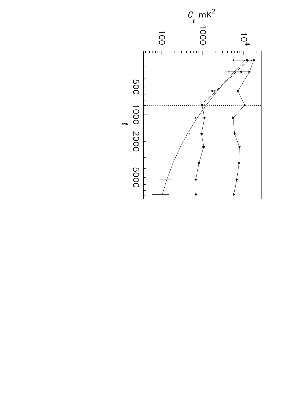
FIELD I was centered at sky position with ${\rm RA}\ =\ 05\ {\rm h}\ 30\ {\rm m}\ 00\ {\rm s}$ and ${\rm Dec}\ =\ +60^{\circ}\ 00^{{}^{\prime}}\ 00^{{}^{\prime\prime}}$ with a frequency bandwidth of $8\,{\rm MHz}$ centered at $150\,{\rm MHz}$, however only a frequency width of $3.75\,{\rm MHz}$ was used for the final analysis. A continuum image of the field was first used to identify point sources to a limiting flux of $10\,{\rm mJy}$. This corresponds to $\sim 7$ times the off-source RMS. noise of $1.3\,{\rm mJy/beam}$ obtained in the continuum image. The point sources were subtracted from the visibility data, and the residual visibilities were used for the subsequent analysis.

The TGE was applied to the visibility data to estimate the angular power spectrum $C_{\ell}$ both before and after the point sources were subtracted. The analysis used the value $f=0.8$ for the tapering parameter. The results are shown in Figure 2 which has been reproduced from Ghosh et al. 2012. It is clearly visible that subtraction of the point sources causes the sky signal to fall considerably at all angular multipoles. The $C_{\ell}$ for the residual data after point source subtraction clearly shows different behaviour in two different ranges of $l$. At low angular multipoles ($\ell\leq 800$), which correspond to angular scales larger than $10^{\prime}$, we find a steep power law behavior which is typical of the Galactic synchrotron emission observed at higher frequencies and larger angular scales (e.g. Bennett et al. 2003). The angular power spectrum flattens out for $\ell>800$, and we find that it remains nearly flat out to $\ell\approx 8,000$ which corresponds to angular scales of $\sim 1^{{}^{\prime}}$. The nearly flat region arises from the residual point sources which have a flux below the threshold for source identification, and hence have not been subtracted from the data. There is also a contribution from the residuals arising from errors in modelling the brighter point sources. The residual point source contribution dominates $C_{\ell}$ at small angular scales where we are unable to make out the Galactic synchrotron radiation.

It is clear from this analysis that $C_{\ell}$, after point source subtraction, is dominated by the diffuse Galactic synchrotron emission at $\ell\leq 800$ which corresponds to $\sim 10^{\prime}$. We have used a weighted least square to fit a power law model

to the measured $C_{\ell}$ for $\ell\leq 800$. We find the best fit values $A=513\pm 41\,{\rm mK}^{2}$ and $\beta=2.34\pm 0.28$ for which $C^{M}_{\ell}$ is also shown in Figure 2. Our findings are consistent with those of Bernardi et al. (2009) who have analyzed $150\,{\rm MHz}$ WSRT observations. They have subtracted out point sources above 15 mJy, and used the resulting image to estimate the angular power spectrum $C_{\ell}$ which they find is well described by a power law for $\ell\leq 900$. There has also been considerable work on modelling the Galactic synchrotron radiation at the higher frequencies relevant for the Cosmic microwave background radiation (CMBR) (tens of GHz). These works predict a power law behaviour $C_{\ell}\propto\ell^{-\beta}$ where $\beta$ has values in the range $2.4$ to $3$ down to $\ell=900$ (Tegmark & Efstathiou 1996; Tegmark et al. 2000). Giardino et al. (2002) have analyzed the $2.4\,{\rm GHz}$ Parkes radio continuum survey of total intensity of the southern Galactic plane where they find a slope $\beta=2.37\pm 0.21$ across the range $40\leq\ell\leq 250$. Our slope, measured at smaller angular scales, is consistent with these findings.

As mentioned earlier, the DGSE is the most important diffuse foreground for observations of the cosmological 21-cm signal. The study of the DGSE is also important in its own right as it allows us to probe the cosmic ray electron and magnetic filed distributions in the turbulent ISM of our Galaxy. We now discuss the prospects of measuring the angular power spectrum $C_{\ell}$ of the DGSE using $160\,{\rm MHz}$ observations with the upcoming SKA1 Low. Present measurement of the $C_{\ell}$ of the DGSE at $150\,{\rm MHz}$ are restricted to $\ell\leq\ell_{max}=900$, the signal at larger angular multipoles is dominated by the residual point sources after point source subtraction. It is anticipated that future observations with SKA1 Low will allow the point sources to be identified and subtracted down to a lower limiting flux $S_{c}$ than possible in the earlier observations described here. This should, in turn, allow us to measure the $C_{\ell}$ of the DGSE out to a larger value of $\ell_{\max}$ thereby allowing us to probe the structure of the turbulent ISM at smaller angular scales than those possible in earlier observations.

Table 6 of Prandoni and Seymour (2015) shows that one expects to achieve a $5\,\sigma$ noise level of $\sim 6\,\mu{\rm Jy}$/beam in $\sim$ 8 hours of observation in a single field with SKA1 Low. We use this to estimate the limiting flux $S_{c}$ for future SKA1 Low observations, assuming that all sources above the $5\,\sigma$ noise level can be identified and subtracted. We further assume that the $5\,\sigma$ noise level falls inversely as the square-root of the observing time, and therefore the limiting flux can lowered by having longer observations. We use this to model the angular power spectrum $C_{\ell}$ of the sky signal as the value of $S_{c}$ is lowered (Figure 3). Our prediction for $C_{\ell}$ incorporates the two most dominant components, namely the point sources and the DGSE. The model prediction for the DGSE is based on the angular power spectrum $C_{\ell}^{M}$ (eq. 5) measured in 150 MHz GMRT observation (Ghosh et al. 2012). Point sources make two distinct contributions to the angular power spectrum, the first being the Poisson fluctuation due to the discrete nature of the sources and the second arising from the clustering of the sources. The point source contribution is predicted using the differential source count measured at 150 MHz (Ghosh et al. 2012) and a power law index of $1.1$ for the angular two-point correlation $\omega(\theta)$ at $1.4\,{\rm GHz}$ (Cress et al. 1996). For the purpose of the predictions, the DGSE contribution has been extrapolate from $150\,{\rm MHz}$ to $160\,{\rm MHz}$ using a mean spectral index of 2.52 from Rogers & Bowman (2008). Similarly, we have extrapolated the point source contribution to $160\,{\rm MHz}$ using a average spectral index of $2.7$ (Jackson 2005; Randall et al. 2012). The framework for modelling the expected $C_{\ell}$ has been presented in detail in Ali, Bharadwaj & Chengalur (2008).

The left panel of Figure 3 shows the total point source contribution to $C_{\ell}$ predicted for three different values of the limiting flux $S_{c}=10\,\mu{\rm Jy}$, $20\,\mu{\rm Jy}$ and $50\,\mu{\rm Jy}$ respectively. The two horizontal dotted lines show just the Poisson contribution for $S_{c}=10\,\mu{\rm Jy}$ and $50\,\mu{\rm Jy}$ respectively. The Poisson contribution falls very rapidly as $S_{c}$ is lowered, and we see that the Poisson component is sub-dominant to the clustered component at all values of $\ell$ for the $S_{c}$ values which we have considered here. The DGSE contribution shown in Figure 3 does not change with $S_{c}$. We see that the DGSE is the most dominant component at $\ell\leq\ell_{max}=2\times 10^{4}$ and $\ell\leq\ell_{max}=5\times 10^{4}$ for $S_{c}=$ 50 $\mu{\rm Jy}$ and 10 $\mu{\rm Jy}$ respectively. We clearly see that future observations with the upcoming SKA1 Low are expected to probe the DGSE at angular multipoles which are much larger than those where we currently have measurements.

The right panel of Figure 3 shows how the value of $\ell_{max}$ changes as the value of $S_{c}$ is varied. The largest angular multipole where we currently have measurements of the DGSE is around $\ell_{max}\sim 10^{3}$. We see that it is possible to achieve $\ell_{max}\sim 10^{4}$ , i.e. and order of magnitude increase in $\ell_{max}$, with $S_{c}=100\,\mu{\rm Jy}$ which one expects to achieve in approximately $2$ minutes of observation with SKA1 Low. We find that the relation between $\ell_{max}$ and $S_{c}$ is well fitted by the power law $\ell_{\rm max}=58000\,({\rm S}_{c}/10\,\mu\rm Jy)^{-0.55}$. This power law implies that we expect ${\ell}_{max}$ to increase as $t^{0.275}$ as the observing time $t$ is increased, and we can expect to achieve $\ell_{max}\sim 10^{5}$ in approximately $10$ hours of observation.

In conclusion we note that present measurement of the angular power spectrum $C_{\ell}$ of the diffuse Galactic synchrotron emission are restricted to $\ell\leq l_{max}\sim 10^{3}$. Future observations with the upcoming SKA1 Low are expected to allow us to probe this at much larger multipoles. Our predictions show that one expects to achieve $\ell_{max}$ in the range $10^{4}$ to $10^{5}$ using observations that span a few minutes to tens of hours in duration.

We thank an anonymous referee for useful comments and suggestions. SC would like to acknowledge the University Grant Commission (UGC), India for providing financial support through Senior Research Fellowship. SSA would like to acknowledge C.T.S, I.I.T. Kharagpur for the use of its facilities. SSA would also like to thank the authorities of the IUCAA, Pune, India for providing the Visiting Associateship programme.

References

- [1] [] Ali S. S., Bharadwaj S.,& Chengalur J. N., 2008, MNRAS, 385, 2166
- [2] [] Begum, A., Chengalur, J. N., & Bhardwaj, S. 2006, MNRAS, 372, L33
- [3] [] Bennett A. S., 1962, MNRAS, 125, 75
- [4] [] Bernardi, G., de Bruyn, A. G., Brentjens, M. A., et al. 2009, A & A, 500, 965
- [5] [] Bharadwaj, S., Nath, B.B. and Sethi, S.K., 2001,JApA,22,21
- [6] [] Chapman, E., Zaroubi, S., Abdalla, F., et al. 2014, arXiv:1408.4695
- [7] [] Choudhuri, S., Bharadwaj, S., Ghosh, A., & Ali, S. S., 2014, MNRAS, 445, 4351
- [8] [] Choudhuri, S., Bharadwaj, S., Roy, N., Ghosh, A., & Ali, S. S., 2016a, MNRAS, 459, 151
- [9] [] Choudhuri, S., Roy, N., Bharadwaj, S., Ali, S. S., Ghosh, A., & Dutta, P. 2016b, submitted to MNRAS
- [10] [] Choudhuri, S., Bharadwaj, S., Chaterjee, S., Ali, S. S., Roy, N., Ghosh, A., & Ali, S. S., 2016c, submitted to MNRAS
- [11] [] Cress, C. M., Helfand, D. J., Becker, R. H., Gregg, M. D., White, R. L. 1996, ApJ, 473, 7.
- [12] [] Dutta P., Begum A., Bharadwaj S., & Chengalur J. N. 2009, MNRAS, 398, 887
- [13] [] Ghosh, A., Bharadwaj, S., Ali, S. S., & Chengalur, J. N. 2011a, MNRAS, 411, 2426
- [14] [] Ghosh, A., Bharadwaj, S., Ali, S. S., & Chengalur, J. N. 2011b, MNRAS, 418, 2584
- [15] [] Ghosh, A., et al. 2012, MNRAS, 426, 3295
- [16] [] Giardino G., Banday A. J., Fosalba P., Gorski K. M., Jonas J. L., O’Mullane W., Tauber J., 2001, A&A, 371, 708
- [17] [] Giardino G., Banday A. J., G ’orski K. M., Bennett K., Jonas J. L., Tauber J., 2002, A&A, 387, 82
- [18] [] Iacobelli, M., Haverkorn, M., Orrú, E., et al. 2013, A & A, 558, A72
- [19] [] Jackson C., 2005, PASA, 22, 36
- [20] [] Koopmans, L., Pritchard, J., Mellema, G., et al. 2015, Advancing Astrophysics with the Square Kilometre Array (AASKA14), 1
- [21] [] Lazarian, A., & Pogosyan, D. 2012, Ap.J, 747, 5
- [22] [] Liu, A., & Tegmark, M. 2012, MNRAS, 419, 3491
- [23] [] Mellema, G., et al. 2013, Experimental Astronomy, 36, 235
- [24] [] Morales, M. F., & Wyithe, J. S. B. 2010, ARAA, 48, 127
- [25] [] Paciga G. et al., 2011, MNRAS, 413, 1174
- [26] [] Pober, J. C., Hazelton, B. J., Beardsley, A. P., et al. 2016, Ap.J, 819, 8
- [27] [] Prandoni, I. and Seymour, N.: 2015, Advancing Astrophysics with the Square Kilometre Array (AASKA14) p. 67
- [28] [] Pritchard, J. R. and Loeb, A.: 2012, Reports on Progress in Physics 75(8), 086901
- [29] [] Randall, K. E., Hopkins, A. M., Norris, R. P., et al. 2012, MNRAS, 421, 1644
- [30] [] Rogers, A. E. E., Bowman, J. D. 2008, ApJ, 136, 641
- [31] [] Seljak, U., 1997, Ap.J, 482, 6
- [32] [] Swarup, G., Ananthakrishnan, S., Kapahi, V. K., Rao, A. P., Subrahmanya C. R., Kulkarni, V. K. 1991, Curr. Sci., 60, 95.
- [33] [] Tegmark M., Efstathiou G., 1996, MNRAS, 281, 1297
- [34] [] Tegmark M., Eisenstein D. J., Hu W., de Oliveira-Costa A., 2000, ApJ, 530, 133
- [35] [] Thyagarajan, N., Udaya Shankar, N., Subrahmanyan, R., et al. 2013, Ap.J, 776, 6
- [36] [] Trott, C. M., Wayth, R. B., Macquart, J.-P. R., & Tingay, S. J. 2011, Ap.J, 731, 81
- [37] [] van Haarlem, M. P., Wise, M. W., Gunst, A. W., et al. 2013, A & A, 556, A2
- [38] [] Waelkens, A. H., Schekochihin, A. A., & Enßlin, T. A. 2009, MNRAS, 398, 1970