A Variational principle for a non-integrable model
Abstract.
We show the existence of a variational principle for graph homomorphisms from to a -regular tree. The technique is based on a discrete Kirszbraun theorem and a concentration inequality obtained through the dynamics of the model. As another consequence of the concentration inequality we also obtain the existence of a continuum of translation-invariant ergodic gradient Gibbs measures for graph homomorphisms from to a regular tree. The method is sufficiently robust such that it could be applied to other discrete models with a quite general target graphs.
Key words and phrases:
Variational principles, non-integrable models, limit shapes, domino tilings, Glauber dynamics, Azuma-Hoeffding, gradient-Gibbs measures, entropy, concentration inequalities, ergodic measures.2010 Mathematics Subject Classification
Primary: 82B20, 82B30, 82B41, Secondary: 60J10.1. Introduction
The appearance of limit shapes as a limiting behavior of discrete systems is a well-known and studied phenomenon in statistical physics and combinatorics (e.g. [Geo88]). Among others, models that exhibits limits shapes are domino tilings and dimer models (e.g. [Kas63, CEP96, CKP01]), polymer models, random tiling models in particular lozenge tilings (e.g. [Des98, LRS01, Wil04]), Gibbs models (e.g. [She05]), the Ising model (e.g. [DKS92, Cer06]), asymmetric exclusion processes (e.g. [FS06]), random matrices (see e.g. [Wig59, KS99]), sandpile models (e.g. [LP08]), the six vertex model (e.g. [BCG16, CS16, NR16]), Young tableaux (e.g. [LS77, VK77, PR07]).
Limit shapes appear in stiff systems whenever a boundary condition forces a certain response of the system. The main tool to explain limit shapes is a variational principle. The variational principle asymptotically characterizes the number of microscopic states i.e. the microscopic entropy , via a variational problem. This means that for large system sizes , the entropy of the system is given by maximizing a macroscopic entropy over all admissible limiting profiles . The boundary conditions are incorporated in the admissibility condition. In formulas, the variational principle can be expressed as (see for example Theorem 2.12 below)
| (1) |
where the macroscopic entropy
can be calculated via a local quantity . This local quantity is called local surface tension in this article.
Often, a consequence of a variational principle is that the uniform measure on the microscopic configurations concentrates around configurations that are close to the minimizer of the variational problem (see comments before Theorem 2.14 below). This is related to the appearance of limit shapes on large scales.
In analogy to classical probability theory, one can understand the variational principle as an elaborated version of the law of large numbers. On large scales, the behavior of the system is determined by a deterministic quantity, namely the minimizer of the macroscopic entropy. Hence, deriving a variational principle is often the first step in analyzing discrete models, before one attempts to study other questions like the fluctuations of the model.
A lot of inspiration for this article comes from the variational principle for domino tilings [CKP01] (see Figure 1(a)). It is one of the fundamental results for studying domino tilings and the other integrable discrete models. A detailed analysis of the limit shapes for domino tilings was given in [KO+07]. Recently a new constructive approach was developed in [CS16] for the determination of the Arctic curve (the frozen boundary of
the limit shape). The approach is discussed mainly in the framework
of the six vertex model, which is integrable. However, the method seems to be very robust. It is an interesting open question if this method can also be used to determine the Arctic curve in a non-integrable model.

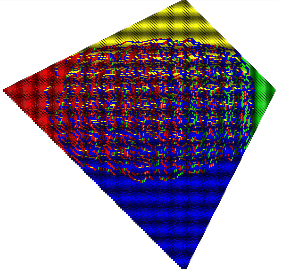

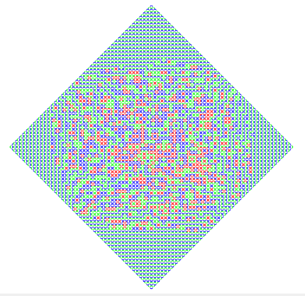
So far, all the tools that were developed to study variational principles of discrete models heavily rely on the intermediate value theorem. Specifically, two valued functions moving at different speed in must meet at some points of the lattice, whose points or clusters provide sets where the value of the two functions can be exchanged. This allows a general technique called cluster swapping (see [She05]) and its variants.
Up to the knowledge of the authors, there is no non-trivial example of a variational principle for which the target space of the underlying model does not have this property. However, simulations (see Figure 1(b), Figure 2(a) and Figure 2(b)) show that limit shapes also appear for discrete maps taking values in a large class of discrete target spaces. The purpose of this article is to go beyond -valued models and to find out what properties of a discrete system lead to variational principles and limit shapes. As a general guideline, we strive to develop a robust method for deducing variational principles for graph homomorphisms that is purely based on general principles of statistical mechanics and not on particular methods for certain classes of graphs, similar to what was developed in [KS99] for the limiting bulk distribution of eigenvalues of random matrices.
We are interested in graph homomorphisms because they provide a natural framework to study systems with hard constraints (see [BW00]) and because they are closely related to other classical model in statistical physics: the loop model (see [DCPSS17]) and tilings by bars (see [Tas14]). In this article, we consider the non-integrable model of graph homomorphisms from to a -regular tree . We want to point out the fact that in our variational principle the underlying lattice can have arbitrary dimension . In the special case of and , our model is equivalent to the six-vertex model with uniform weights (cf. [vB77, CPST18]).
We identified two properties that a model of discrete maps needs to satisfy in order to have a variational principle. The first one is a stability property that allows to glue together pieces of different configurations at a negligible entropic cost. As a consequence, perturbing the boundary condition on a microscopic scale does not change the macroscopic properties of the model. The second one is a concentration property.
In the case of discrete -valued models, such as height functions of domino tilings or the antiferromagnetic Potts model, both properties can be deduced naturally. For deducing the first property, one uses that the space of configurations is a lattice. Then it is possible to quickly attach two configurations together provided that the boundary conditions are similar. This is done by using the minimum of two well-chosen extensions of those configurations. The second property, namely the concentration, is tackled by using a cluster swapping argument or an analog version of this argument for other systems (see e.g. [CEP96, She05]).
We want to emphasize again that those arguments are based on properties which rely on the intermediate value theorem in the target space and are not available for general graph homomorphisms. One of the main contributions of this article is that we provide alternative methods. These methods are not based on integrability but on weaker properties of graphs and of the underlying dynamics of the model. The authors believe that the principles behind those new arguments are robust. They should provide a possible line of attack to study variational principles and limiting behavior of a large class of discrete models.
Now, let us discuss how the two necessary properties, namely stability and concentration, are deduced without relying on integrability. The first property is obtained by using the discrete version of a well-known theorem for continuous metric spaces: the Kirszbraun theorem (see Theorem 3.9 below). This theorem states that any graph homomorphism from a subset of to a regular tree , which is contracting for the graph distances in and , can be extended to the whole space . Up to knowledge of the authors, the first version of a discrete Kirszbraun theorem was developed in the setting of tilings in [Tas14] and [PST16]. Using a new version of the Kirszbraun theorem for graph homomorphisms allows us to show that microscopic variations of the boundary conditions can be neglected on the macroscopic scale and thus do not influence the entropy of a system.
The second property, namely the concentration, is provided in Theorem 3.10. The concentration is deduced via a combination of a classical concentration inequality, namely the Azuma-Hoeffding inequality, with a coupling technique relying on dynamical properties of the model.
Inspiration for this type of argument comes from [CEP96], where the Azuma-Hoeffding inequality was used to show concentration for domino tilings. However, it is very difficult to apply directly the Azuma-Hoeffding inequality for more sophisticated models. This would need detailed information about the structure of the underlying space of configurations. Our dynamical approach circumvents this obstacle. One only has to understand the response of the system to changing the value of one point.
The natural process for our dynamical approach is the Glauber dynamics (see [Cha16] for details). This choice would be fine for studying graph homomorphisms to . However, using the Glauber dynamics does not work for the more complicated model of graph homomorphisms to a tree . Heuristically, this can be understood from the observation that two simple random walks on a tree tend to diverge. We overcome this technical obstacle by two adaptations. On the one hand, we add to the original Glauber dynamics an extra non-local resampling step. On the other hand, we introduce a suitable quantity called depth. It turns out the modified Glauber dynamics conserves this quantity. This allows us to apply the Azuma-Hoeffding inequality and deduce concentration in depth. We then show that concentration in depth is sufficient for deducing our variational principle.
The main ingredients for the proof of a variational principle (see (1) or Theorem 2.12) are the equivalence of the different notions of the local surface tension, that the local surface tension is bounded from below, and that it is convex. For the equivalence, let us have a closer look at the definition of the local surface tension . As usual, the local surface tension is defined as the limit of microscopic entropies on a box with suitable chosen boundary conditions (see Section 3) i.e.
| (2) |
The freedom of choosing different boundary conditions leads to a-priori different notions of the local surface tension. In particular, choosing the boundary condition to be a fixed state with slope leads to the notion of surface tension which is associated to fixed boundary conditions. Allowing the boundary condition to be any state that is close to leads to the notion of surface tension which is associated to fluctuating boundary conditions. Allowing periodic boundary conditions with slope leads to the notion of surface tension which is associated to fluctuating boundary conditions.
A crucial ingredient for deducing a variational principle (1) is that those a-priori distinct notions of the local surface tension are equivalent i.e.
| (3) |
This equivalence is deduced in this article in Theorem 3.12. The argument relies on the two basic properties outlined above, i.e. the Kirszbraun theorem (cf. Theorem 3.9) and the concentration inequality (cf. Theorem 3.10). The existence of the limit is usually deduced via sub-additivity arguments. For example, in [FS97] sub-additivity was exploited to show the existence of the local surface tension the continuous model. In [MKT17] it is shown that sub-additivity combined with the Kirszbraun theorem can be used to show the existence of the local surface tension in homogenization of random surfaces. However, those arguments do not carry over to periodic boundary conditions. Those argument cannot be used to show the a-priori existence of the local surface tension that is associated to periodic boundary conditions. In this article, we show the existence of the via a self-contained argument based on a combination of the Kirszbraun theorem and the concentration inequality (cf. Theorem 3.8 below).
In the same spirit, we also give a self-contained argument that the local surface tension is convex (see Theorem 3.15). From convexity it follows that the variational problem given by our variational principle has a minimizer (cf. Theorem 2.12 below). However, we do not prove that this minimizing limiting profile is unique. The uniqueness of the minimizer would follow if the local surface tension is strictly convex. We do not know if the local surface tension is strictly convex but we conjecture it.
Beside the equivalence (3) and the convexity of (see Theorem 3.15, Theorem 3.12 and Lemma 6.3), the only additional ingredients for the proof of the variational principle are very general principles, namely the compactness of Lipschitz functions on a bounded region and that Lipschitz functions can be very well approximated by piecewise affine functions on a simplicial complex (see Section 6).
Compared to , there are infinitely many ways to travel to infinity in a tree . Those pathways to infinity are described by geodesics. Limit shapes are sensitive to the choice of geodesics on which the graph homomorphism travels on the boundary (see Figure 3 for an illustration). This adds another technical difficulty when deducing the variational principle for graph homomorphisms to a tree. The problem is to define the scaling limit of a graph homomorphism. For domino tilings the height function is an integer valued map, which allows a natural notion of a scaling limit. If the space of geodesics is more complex, as it is the case for trees, the notion of a scaling limit is less obvious. In order to define the scaling limit of a graph homomorphism to a tree one has to additionally keep track of the information on which geodesic the graph homomorphism is traveling on. This leads to a more subtle definition of the limiting profile which involves several compatibility conditions (see Definition 2.3). Another consequence is that the set of admissible limiting profiles , over which the continuous entropy is minimized, has a more elaborated structure involving additional constraints.
In this article, we also discuss another consequence of the Kirszbraun theorem and the concentration inequality. It is the existence of a continuum of shift-invariant ergodic gradient Gibbs measures on tree-valued graph homomorphisms on (see Section 5 and Theorem 5.5). This is also the reason why we choose periodic boundary conditions for defining the local surface tension . This choice allows us to obtain measures which are translation-invariant. A key point for proving the existence of ergodic gradient Gibbs measures is also that the concentration inequality of Theorem 3.10 applies to those translation-invariant measures. Although the statement of Theorem 5.5 does not imply the strict convexity of the local surface tension, we believe that it is a very strong indication that the surface tension must be strictly convex since it shows that different boundary conditions will lead to different phases.

Overview over the article
In Section 2, we outline the precise setting, introduce relevant definitions and state the main result of this article: the variational principle for tree-valued graph homomorphisms (see Theorem 2.12). In Section 3 we discuss the local surface tension associated to the slope . We show the existence of in Theorem 3.8 and the convexity of in Theorem 3.15. Section 4 is dedicated to proving technical lemmas which are central to our main results. Namely, in Theorem 3.9 we prove the Kirszbraun theorem and in Theorem 3.10 we deduce the concentration inequality. This concentration inequality is used in Section 5 to prove the existence of an infinite volume gradient Gibbs measure for each possible slope (see Theorem 5.5). Finally, in Section 6 we give the proof of the variational principle itself.
Notation
- •
and denote generic positive bounded universal constants.
- •
If is finite then denotes the cardinality of the set . If then denotes the Lebesgue measure of the set .
- •
denote elements .
- •
.
- •
denotes the -th Euclidean basis vector.
- •
indicates that the points and are neighbors.
- •
is the oriented edge from to .
- •
distance in the graph .
- •
denotes a -regular tree.
- •
denote elements .
- •
denotes the root of the tree .
- •
denotes a geodesic of the tree .
- •
is the projection on the geodesic .
- •
boundary point of the directed geodesic .
- •
.
- •
denotes a generic smooth function with .
- •
denotes colors of edges.
- •
denotes the generating set of a -regular graph.
- •
is a graph homomorphism.
- •
is the set of all graph homomorphisms that are invariant with slope and supported on the geodesic .
- •
is the set of all graph homomorphisms that are invariant with slope and supported on the geodesic such that is pinned at a fixed point.
- •
- •
- •
Since and are both bipartite let us fix a -coloring of the two graphs. The color of a vertex is called parity.
- •
denotes the usual inner product of .
2. The variational principle for graph homomorphisms
Let us start with clarifying the underlying model. We closely follow the setting of [CKP01] with the main difference that we allow the underlying lattice to be dimensional and that we consider graph homomorphism to a regular tree. We equip the -dimensional lattice and with the -norm.
Assumption 2.1.
For each we consider a bounded lattice region (i.e. a connected region composed of squares from the unit square lattice). We assume that for the scaled sub-lattice converges in the Hausdorff distance to a bounded, simply connected, Lipschitz domain .
The basic objective is to study graph homomorphisms , where denotes a regular tree.
Definition 2.2.
(Graph homomorphism, height function) Let denote the d-regular rooted tree and let be a finite set. We denote with the natural graph distance on a graph . A function is called graph homomorphism, if
for all with . In analogy to [CKP01], we may also call a -valued height function. Let denote the inner boundary of i.e.
| (4) |
We call a homomorphism boundary graph homomorphism or boundary height function.
We want to study the question of how many valued height functions exist that extend a fixed prescribed boundary height function . Hence, let us consider the set that is defined as
| (5) | ||||
The goal of the article is to derive an asymptotic formula as of the microscopic entropy
| (6) |
For this purpose, let us introduce the notion of an asymptotic height profile and the notion of an asymptotic boundary height profile. Those two objects will serve as the possible limits of sequences of graph homomorphisms and boundary graph homomorphisms .
Definition 2.3 (Asymptotic height profile).
Let , let be a function and let be a set of non-negative real numbers satisfying the following compatibility conditions
| (7) |
and (cf. Figure 4)
| (8) |
for all . We say that is an asymptotic height profile if:
- •
The first coordinate of the map is 1-Lipschitz with respect to the -norm in , i.e. for all :
(9) - •
The map is -admissible in the sense that for all :
(10)

Compared to a classical asymptotic height function (see for example [CKP01]) our notion of an asymptotic height profile has two coordinates and . Opposed to , there are infinitely many ways to travel from zero to infinity on a tree . Those pathways to infinity are described by directed geodesics starting at the root .
Definition 2.4.
(One- and two-sided geodesics on the tree ) Let denote the -regular tree with root . A graph homomorphism is called one-sided (or directed) geodesic if the map is one-to-one. Two one-sided geodesics and are asymptotic if there are such that
We say that a one-sided geodesic starts in . A graph homomorphism is called two-sided geodesic if the map is one-to-one.
Convention 2.5.
If is a two-sided geodesic on the graph containing the root , we identify with a one-to-one graph homomorphism such that .
We assume that the asymptotic boundary height profile will travel only on finitely many one-sided geodesics that are indexed by and start in the root . This requirement is natural since graph homomorphisms are -Lipschitz. Hence the limiting profile on the boundary of must have finite total variation.
The second coordinate of an asymptotic height profile indicates on which one-sided geodesic the point is mapped to. More precisely, the point will be mapped onto a point on the one-sided geodesic . The first coordinate of the asymptotic boundary profile specifies the exact location on the one-sided geodesic . This means that will be mapped onto a point on the one-sided geodesic that has distance from the root . Working with one-sided geodesics allows to assume that is non negative. The Lipschitz condition (9) on is very natural and follows from the fact that graph homomorphisms are Lipschitz. This is very similar to the setting of classical height functions (see [CKP01]).
Let us now describe the meaning of the numbers appearing in the compatibility condition (8) and the condition (10). The numbers have their origin in the following observation. Any two one-sided geodesics and starting at have a nonzero intersection . However, they must split up at some vertex (see also discussion below and Figure 6). If seen from the root , the vertex can be interpreted as the splitting point of the one-sided geodesics and . If seen from infinity, the vertex can be interpreted as the meeting point of the one-sided geodesics and . The number denotes the asymptotic height of this meeting point (see also (17) in Definition 2.10). When traveling on a geodesic from infinity, it is only possible to change to the other geodesic by passing through the meeting point . The admissibility condition (10) enforces that the asymptotic height profile has a similar property. Using this interpretation of the number it also becomes clear why the compatibility condition (8) is needed (see also Figure 4). This interpretation is made precise in the following lemma.
Lemma 2.6.
The statement of Lemma 2.6 is not used later in the article. The proof is straight-forward and is therefore omitted in the article. Let us consider an example and assume that there are points such that the second coordinate and . This indicates that the asymptotic height function travels at on the one-sided geodesic and at on the one-sided geodesic . Now, let us consider a path from to . Then the asymptotic height function has to change geodesics on that path. The admissibility condition (10) enforces that changing from the one-sided geodesic to the one-sided geodesic can only take place below the meeting point, which is characterized by the height . We also want to note that if then the second coordinate is allowed to change freely between and with no regularity condition. Below the height the geodesics and are indistinguishable.

For an illustration of an asymptotic height profile we refer to Figure 5. On the blue region , the height profile travels on the one-sided geodesic . On the red region , the height profile travels on the one-sided geodesic . Mathematically, this means that the second coordinate of satisfies
| (12) |
The yellow line separates the blue region and the red region . The admissibility condition (10) means that one can only cross from to below the meeting point of and . Hence, the first coordinate of satisfies for all
| (13) |
In a variational principle only the boundary condition is prescribed. For that reason, we now adapt Definition 2.3 and define the notion of an asymptotic boundary height profile.
Definition 2.7 (Asymptotic boundary height profile).
Compared to the Definition 2.3 of an asymptotic height profile, the condition (14) is new. It is needed to guarantee that every asymptotic boundary height profile can be extended to an asymptotic boundary height function.
Lemma 2.8.
Let be an asymptotic boundary height function in the sense of Definition 2.7. Then it can be extended to an asymptotic height profile on the full region .
The proof of Lemma 2.8 is stated in Section 6. Lemma 2.8 is important because otherwise the statement of the variational principle, formulated in Theorem 2.12 below, could be empty.
The next step towards the variational principle is to define in which sense a sequence of (boundary) graph homomorphisms converges to an asymptotic height profile . For this purpose let us introduce some necessary definitions.
Definition 2.9.
(Boundary points (cf. [Klo08])) A boundary point is an equivalence class of asymptotic one-sided geodesics. We denote with the boundary point associated to an one-sided geodesic i.e. . We denote with the set of all boundary points. We observe that each boundary point has a canonical representative such that is a one-sided geodesic starting at the root i.e. . Because a two-sided geodesic is the union of two one-sided geodesics and , the two-sided geodesic has two boundary points which we denote with and .
It follows from the definition that for two boundary points , there is a unique element such that (cf. Figure 6)
| (15) |
where and are the canonical representatives of and (cf. Definition 2.9). We will write
| (16) |
and call the height of the meeting point of the two one-sided geodesics and .
We are now ready to define the convergence of a sequence of boundary graph homomorphisms to an asymptotic boundary height profile.
Definition 2.10.
Let be a sequence of boundary height functions and let be an asymptotic boundary height profile in the sense of Definition 2.7. We say that the sequence converges to (i.e. ), if the following conditions are satisfied:
- •
For all .
- •
- •
For we define the set
(18) Then it holds that
(19) (20) where and are the two components of the map .
Definition 2.10 is illustrated in Figure 6. The condition (17) ensures that the quantity characterizes the asymptotic meeting point of the one-sided geodesics and . One can observe that the compatibility condition (8) on is actually a consequence of the condition (17). The condition (19) asymptotically characterizes the values of graph homomorphism via the asymptotic height profile.
Before we turn to the main result of this article let us introduce the local surface tension for .
Theorem 2.11.
(The local surface tension.) Let be a two-sided geodesic satisfying and let . For satisfying , let be the boundary graph homomorphism given by
Then the limit in the following equation exists and defines the local surface tension :
| (21) |
If we define .
This notion of surface tension is associated to fixed boundary condition. The proof of Theorem 2.11 is given in Section 3.1. There, we will also show the equivalence of the notion of local surface tension wrt. different boundary conditions (cf. (3)). Contrary to the case of random domino tilings, we do not have an explicit formula for the local surface tension . In Section 3.1 we also deduce the convexity of the local surface tension . In analogy to random domino tilings, the authors believe that the local surface tension is strictly convex, but they are missing a proof.
Let us now formulate the main result of this article, namely the variational principle for graph homomorphisms to a regular tree. As we outlined in the introduction, a variational principle contains two statements. The first statement, namely Theorem 2.12, gives a variational characterization of the entropy (cf. (6))
Hence, it asymptotically characterizes the number of possible graph homomorphisms with boundary data .
Theorem 2.12 (Variational principle).
Under the Assumption 2.1, we assume that the boundary height functions converge to an asymptotic boundary height profile in the sense of Definition 2.10. Let denote the set of asymptotic height profiles that extend from to . Given a 1-Lipschitz function defined on , we define the macroscopic entropy via
| (22) |
where the local surface tension is given by Theorem 2.11. Then it holds that
| (23) |


Because the function is Lipschitz by Definition 2.3, the gradient exists almost everywhere by Rademacher’s theorem. Because the local surface tension is bounded from below and convex we know that the variational problem (23) has a minimizer. However, we do not know if the minimizer of the surface tension is unique.
Let us now turn to the second part of the variational principle, namely the profile theorem (see Theorem 2.14 from below). The profile theorem contains information about the profile of a graph homomorphisms that is chosen uniformly at random from . Heuristically, the statement of the profile theorem is the following. Let us consider an asymptotic boundary height profile . Then the macroscopic entropy is given by the number of graph homomorphisms that are close to . Applying this statement to the minimizer of the continuous entropy has the following consequence. The uniform measure on the set of graph homomorphisms concentrates on graph homomorphisms that have a profile that is close to . As a consequence, a uniform sample of will have a profile that is close to the minimizing profile for large .
Let us now make this discussion precise. For that purpose, we have to specify when the profile of a graph homomorphism is close to an asymptotic height profile .
Definition 2.13.
For fixed and integer , we define the simplicial lattice with -spacing at scale to be the union of the boundary of the simplices defined by
| (24) | ||||
| (25) |
for permutation of size and (see Figure 7). In other words, is the set of points in for which all of the inequalities in (24) are satisfied for a fixed -uplet and at least one of them is an equality.
For a given asymptotic height profile , we define the ball of size on the scale by the formula
| (26) | ||||
| (27) |
where the set of graph homomorphisms is given by (5).

Informally, is the set of all graph homomorphisms which stays within of the rescaled function on the boundary on the rescaled lattice . Now, let us formulate the profile theorem.
Theorem 2.14.
(Profile theorem) Let be an extension of the asymptotic boundary height profile . Then
| (28) |
where is a family of functions indexed by such that for fixed and is a function such that .
Remark 2.15.
We want to point out that the second coordinate does not play a role in the definition (26) of . This means that we neglect the information which one-sided geodesic a graph homomorphism follows, because the entropic effect of choosing the geodesics is of lower order. Rigorously, this fact is deduced in Lemma 6.3 below. Here, let us give a heuristic argument. The variational principle lives on the scale . Approximating the set by blocks of side length it follows that , where is the number of blocks. Having a close look at the definition (26) of shows that only the grid is important. Hence, the entropic effect of choosing different geodesics lives at most on the scale of the length of the lattice . The length of the lattice is of the order and therefore negligible on the scale of the variational principle.
Remark 2.15 shows that choosing different one-sided geodesics and meeting points has no effect on Theorem 2.14. However, it still has an effect on the variational principle formulated in Theorem 2.12. Choosing different geodesics and meeting points changes the set of asymptotic height functions over which the continuous entropy is minimized. This is another main aspect of how the variational principle of Theorem 2.12 is distinct from the variational principle for domino tilings [CKP01].
The proofs of the variational principle (see Theorem 2.12) and of the profile theorem (see Theorem 2.14) are given in Section 6. The profile theorem is deduced first and then used for verifying the variational principle via a compactness argument. The second main ingredient in the compactness argument is that the variational problem on the right hand side of (23) has a minimizer, which follows from the fact that the local surface tension is convex and bounded from below (see Section 3 and Theorem 3.15).
Let us now explain the main idea for deducing the profile theorem. One observes that Lipschitz functions can approximated very well by piecewise affine function on a simplicial complex. This observation heuristically yields that the profile theorem only needs to be verified for a simplicial complex and a piecewise affine profile . Here, we want to recall that simplicial complex means that is a union of finitely many simplices . The desired estimate (28) is deduced in two steps. In the first step one underestimates the number of possible configurations, establishing one direction of the desired (in-)equality. In the second step one overestimates the number of possible configurations, establishing the other direction of the desired (in-)equality.
Let us now describe how the underestimation works. Instead of looking at all possible graph homomorphisms that are close to the profile , one only considers those that match the profile exactly on the boundaries of the individual simplices . By this procedure the simplices become independent of each other. Hence, the entropy of the simplicial complex is bigger then the sum of the entropy of the individual simplices with fixed linear boundary data.
For overestimating the number of configuration on , we allow the values of the graph homomorphisms on to be chosen independent from each simplex, as long as they do not fluctuate too much from the affine profile . Hence, configurations again become independent on each simplex. Therefore, the entropy of the simplicial complex is smaller then the sum of the entropy of the individual simplices with fluctuating linear boundary data.
The only missing ingredient is that on a simplex the entropy with fluctuating linear boundary data is equivalent to the entropy with fixed linear boundary data. This fact is provided in Lemma 6.3 as a consequence of the equivalence of the local surface tension, i.e. that the microscopic entropy on a box with fixed or fluctuating boundary conditions agree (see discussion in the introduction and Theorem 3.12). For the proof of Theorem 3.12 we need two crucial technical results, namely the Kirszbraun theorem (see Theorem 3.9) and the concentration inequality (see Theorem 3.10) which are provided in Section 4.
3. The local surface tension
It is well known that there are many equivalent definitions of the local surface tension (see e.g [She05]). The most simple framework to show the existence is to define the surface tension as the limit of a microscopic entropy on a box with canonical, fixed, linear boundary conditions, as it is done in Theorem 2.11. In this framework the existence follows easily from subadditivity and Feteke’s lemma. One of the most important ingredients for the proof of a variational principle is that the local surface tension is robust to changes in the boundary conditions (see Theorem 3.12 below). In this article, we show that this robustness is a consequence of a combination of the Kirszbraun theorem and of the concentration inequality. In principle, we could proceed in this framework and deduce the concentration inequality on a box for a fixed canonical boundary data.
However, in this article we also show another application of the concentration inequality: It is the existence of a continuum of ergodic gradient Gibbs measures. In order to deduce this result, we need concentration on the level of translation invariant boundary data. To avoid deducing the concentration inequality for two different spaces, we chose to define the local surface tension via the limit of -translation invariant boundary data. This will lead to the notion of local surface tension associated to periodic boundary conditions, denoted in the introduction with . In Theorem 3.8 we show the existence of . A consequence of Theorem 3.12 is that the local surface tension and agree, justifying the existence of a-posterior. This also shows that the local surface tension is a universal object. To be self-contained, our argument of the existence does not use subadditivity but relies on our two main technical ingredients, namely the Kirszbraun theorem and the concentration inequality.
In Section 3.1, we give the precise definition of the microscopic surface tension associated to -translation invariant boundary data and deduce some important auxiliary results. In Section 3.2, we show the existence of the local surface tension as the limit of the microscopic surface tension (see Theorem 3.8 from below). We also show that , which deduces Theorem 2.11. In Section 3.3, we deduce the convexity of the local surface tension (see Theorem 3.15 from below).
3.1. Definition of the microscopic surface tension associated to periodic boundary data
We use a similar approach as in [CKP01] and define the local surface tension as the limit of a microscopic surface tension , i.e.
| (29) |
In order to define the microscopic surface tension associated to periodic boundary data let us study the translation invariant measures of our model. For this reason, we start with generalizing the notion of periodicity of height functions to graph homomorphisms. For this purpose, we will identify the -regular rooted tree with the group
This is done through the natural bijection induced by the Cayley graph of generated by the ’s. We use the convention that the root of is represented by the identity of . The reason for this identification is that the group structure provides an easy way to define gradient measures. Using the previous bijection we can choose a canonical way to associate a unique to each edge of . As a consequence, there is a natural way to associate to a graph homomorphism a dual function acting on edges of :
Definition 3.1 (Dual of a graph homomorphism).
Let be a graph homomorphism. We define its dual map
in the following way. Note that for any there is a unique such that . Then, the value of the dual function on the edge is given by .
The dual map is the gradient map associated to and determines the graph homomorphism up to translations in the graph . If there is no source of confusion, we will denote the dual map and the graph homomorphism with the same symbol .
The dual map maps each path in onto a word in the alphabet and it is not hard to see that this word only depends on the first and last vertex of the path . We will use the notation for the word corresponding to a path between and .
Let us now define the analog of periodicity for graph homomorphisms.
Definition 3.2 (-translation invariant graph homomorphism).
We denote by the -th vector of the standard basis of . Let be a graph homomorphism. We say that is -translation invariant if for all and
Remark 3.3.
If we denote by the shift by in then is -translation invariant iff is -translation invariant.
In order to define the microscopic surface tension we need to associate to every -translation invariant homomorphism a slope which indicates the speed at which the homomorphism travels on the graph in every direction of the plane.
Definition 3.4 (Slope of a translation invariant graph homomorphism).
Let be a -translation invariant homomorphism. The slope of is defined by
An essential property of -translation invariant homomorphisms is that, if the slope is nonzero, they must stay within finite distance of a unique two-sided geodesic of or, if the slope is zero, stay within finite distance of a single point. This statement is made precise in the next lemma.
Lemma 3.5.
Let be a -translation invariant homomorphism with slope . Then there exist a unique two-sided geodesic such that for all
| (30) |
In this case we say that is supported on the two-sided geodesic .
If has slope then has finite range, and for all
| (31) |
Proof of Lemma 3.5.
We start with considering the case where the slope of is . In this case the -invariance yields that for and there exist such that:
Using the translation invariance we obtain that for all :
| (32) | |||||
| (33) |
This yields that for
Now, the estimate (31) follows directly from the observation that any point is within graph distance of the set
Consider now the case where the slope of is not zero. We start by noticing that any two-sided geodesic that satisfies (30) must be unique. Indeed, since is hyperbolic, two geodesics cannot stay within bounded distance of each other. As a consequence can only stay within bounded distance of at most one two-sided geodesic .
Let us now deduce the estimate (30). Let be a non-zero coefficient of the slope . W.l.o.g. generality we assume that . Let us choose such that and let us define .
Along the line in with equation the map travels with speed on the only two-sided geodesic which goes through all the vertices such that the path between and is for . Moreover, since is -periodic we can make the same observation if we replace by one of the points where . For each one of those points we obtain that along the line with equation the map travels with speed on a two-sided geodesic .
Since any two of those lines stays within bounded distance of each other, any two-sided geodesics in must also stay within bounded distance of each other. Hence we deduce that for all . As a consequence we also deduce that for all , the vertex is on where .
Now, let be arbitrary, we can write for some numbers and for . Since graph homomorphisms are -Lipschitz, we obtain that
which is the desired estimate (30). ∎
Definition 3.6 (Microscopic surface tension ).
Let be a periodic two-sided geodesic. For with let us denote by the set
| (35) | ||||
| with slope supported on and | (36) | |||
| if and | (37) | |||
| (38) |
where denotes the projection onto the two-sided geodesic .
The microscopic surface tension is defined as
| (39) |
We denote by the uniform probability measure on . We also define
| (40) | ||||
| (41) |
Remark 3.7.
Because all two-sided geodesics are isomorphic, the definition of is independent from the particular choice of . In particular by re-orientating the geodesic we assume wlog. that . The second and third condition in the definition of anchors the height/depth of the graph homomorphisms on the geodesic . As a consequence, the space is finite. The parity condition on the anchoring comes from the fact that graph homomorphisms conserve the parity. For the precise definition of depth we refer to Definition 4.3.
We note that the Definition 3.6 of is well posed, i.e. the set is not empty. Indeed, one can easily construct elements of by using the Kirszbraun theorem for graphs (see Theorem 3.9 from below). The space does not play a further role in Section 3 but will become important for the proof of the concentration inequality in Section 4.2.
3.2. Existence of the local surface tension
In this section, we show that the limit (29), defining the local surface tension associated to periodic boundary data.
Theorem 3.8.
Let such that and let be given by Definition 3.6. Then the limit
| (42) |
exists and defines the local surface tension . For we define
In this section, we also show another result which is fundamental not only for the proof of Theorem 3.8 but also for deducing the variational principle. It is the robustness of the local surface tension with respect to changes in the boundary condition (see Theorem 3.12 below). A combination of Theorem 3.8 and Theorem 3.12 immediately yields the statement of Theorem 2.11 and shows the identity
| (43) |
In the remaining article, let us follow the convention that denotes the notion of local surface tension associated to periodic boundary data.
The proof of Theorem 3.8 and the proof of Theorem 3.12 uses the following two ingredients. The first ingredient is a Kirszbraun theorem for graphs. It states under which conditions one can attach together two different graph homomorphisms.
Theorem 3.9 (Kirszbraun theorem for graphs).
Let be a connected region of , be a subset of and be a graph homomorphism which conserves the parity. There exists a graph homomorphism such that on if and only if for all in
| (44) |
The second ingredient is a concentration inequality. It states that, for canonical boundary data, a graph homomorphism cannot deviate too much from a linear height profile.
Theorem 3.10 (Concentration inequality).
There exists universal constants and such that, under the uniform measure on , for all in , and for all we have
| (45) |
where is a two-sided geodesic and the map is given by Convention 2.5.
The first step towards the proof of Theorem 3.12 is the following statement, which shows that the microscopic surface tension is not oscillating wildly between two values with ratio close to .
Lemma 3.11.
Let be such that , let and let be three integers such that . Then the following inequality holds
| (46) |

Proof of Lemma 3.11.
Before starting the argument let us recall the definition of . It is defined via
| (47) |
Since and have symmetric roles in the statement of Lemma 3.11, it is sufficient to show that:
| (48) |
Set , our first step is to show that for large the size of the set is comparable to the set
| (49) |
This is a direct consequence of the concentration inequality (45) of Theorem 3.10 which yields that for some universal
| (50) |
This implies that for large enough
| (51) |
Because is the uniform measure on , this yields that for all sufficiently large
| (52) |
For the second step of the argument, let us assume that the box and the box have the same center (see Figure 8). We will show that
| (53) |
Let . For all , and large enough it holds
| (54) | ||||
| (55) |
where in the last inequality we used that:
Using the Kirszbraun theorem, this implies that the restriction of to the box can be extended to the homomorphism defined by on . Additionally, we observe that there are less than many ways to extend a configuration on to the boundary where represents an upper bound on the maximal volume of the box difference . This yields the desired estimate
| (56) |
By combining the estimates (51) and (56) we obtain that
| (57) |
Now if we take the logarithm and divide both sides by , we can rewrite (57) as
| (58) | ||||
| (59) | ||||
| (60) |
where we used that and to go from the third to the last line in the previous inequality. This gives us the desired estimate and finishes our proof. ∎
Another ingredient for the proof of Theorem 3.8 is that the microscopic entropy with -translation invariance and fixed boundary conditions are equivalent:
Theorem 3.12.
Proof of Theorem 3.12.
In order to deduce the desired statement it suffices to show that
| (63) |
and
| (64) |
We start with deducing the estimate (63). We set . It follows from the concentration estimate of Theorem 3.10 that
| (65) |
where denotes the uniform measure on . Let us define the set according to
| (66) |
Then it follows from (65) that
| (67) |
By taking the logarithm and dividing by in the previous equation we obtain
| (68) |
We observe that due to (61) and the Kirszbraun theorem (cf. Theorem 3.9) any element can be extended to a graph homomorphism such that on and on . This implies that for large enough
| (69) | ||||
| (70) | ||||
| (71) |
where we have used the estimate (68) from above and the identity
| (72) |
which follows from Lemma 3.11 applied with the parameters and for large enough . This verifies the estimate (63).
The merit of Theorem 3.12 is the following: In order to show that the limit exists it suffices to show that the limit
exists. The advantage of considering is that the boundary data is fixed and can be chosen such that (61) is satisfied. For a well chosen configuration one could now show the existence of the limit using subadditivity. However, for being self-contained let us give an alternative argument. From now on, let us fix one particular sequence of boundary data that additionally to (61) also satisfies the following condition.
Definition 3.13.
(Periodic boundary data) Let denote a boundary graph homomorphism on the boundary of the box . Let denote the dual boundary graph homomorphism on the edge set of (see Definition 3.1). We say that the boundary graph homomorphism has well-periodic boundary data if the following two conditions are satisfied:
- •
If and for some , then .
- •
If and for some , then .
The Definition 3.13 has the following simple interpretation. The dual boundary graph homomorphism can be understood as a coloring of the edges of the set . Then the boundary data is periodic, if the coloring of one face of matches the coloring of the opposite face.
The advantage of using periodic boundary data is that one gets monotonicity of a subsequence of for free.
Lemma 3.14.
Under the same assumptions as in Theorem 3.12, let us consider the entropy . We additionally assume that the boundary graph homomorphism is periodic in the sense of Definition 3.13. On the box we consider the boundary condition that arises from attaching copies of to each other. Then it holds that for all integers
| (73) |
The proof of Lemma 3.14 follows from a simple underestimation of the configurations in . Because the boundary data is periodic one can just take a configuration on and extend it to the box by attaching copies of to each other. By construction, the resulting configuration on will have the correct boundary data and therefore the estimate (73) follows automatically. We omit the details of this proof.
Now, we have everything that is needed for the proof of Theorem 3.8.
Proof of Theorem 3.8.
The main idea is to consider a sequence of periodic boundary data (see Definition 3.13) that satisfies (61) and show that
| (74) |
Then it easily follows from statement of Theorem 3.12 that also
| (75) |
This would verify the statement of Theorem 3.8.
We begin with observing that
| (76) |
The reason is that edges take at most -values. Therefore, it suffices to show that the sequence cannot have two distinct accumulations points and . We argue by contradiction and assume that and are two accumulation points of the sequence satisfying the relation
Then there exists a number such that
| (77) |
By Lemma 3.14, the subsequence is decreasing, hence for all
| (78) |
We will now show that this implies for large enough and that also for all
| (79) |
for some small constant . This would be a contradiction to the assumption that and are accumulation points of the sequence and therefore would verify (74).
Hence, it is left to deduce the estimate (79). Let . Then we know that we can write
| (80) |
where and . By using a combination of Theorem 3.12 and Lemma 3.11 with parameters and , it follows that
| (81) | ||||
| (82) |
Hence, we see that if choosing large enough and small enough that
| (83) |
which verifies (74) and closes the argument. ∎
3.3. Convexity of the local surface tension
Once the existence of the local surface tension is established it is natural to ask if the local surface tension is convex. This is the case in our model.
Theorem 3.15.
The local surface tension given by Definition 3.6 is convex in every coordinate. In particular, this implies that is convex.
As in the proof of the existence of the local surface tension , the main tools for the proof of Theorem 3.15 are the Kirszbraun theorem (see Theorem 3.9) and the concentration inequality (see Theorem 3.10).
Proof of Theorem 3.15.
We will show that the local surface tension is convex in every coordinate which yields that is convex. By symmetry it suffices to show that is convex in the first coordinate. For convenience, we only give the argument for the case . The argument for the general case is similar. For that reason let be fixed. We argue by contradiction. Hence, let us suppose that is not convex in the first coordinate. Then there are numbers such that
| (84) |
and
| (85) |
For an integer we consider the microscopic entropy given by Definition 3.6 i.e.
| (86) |
where denotes a two-sided geodesic in . We want to recall that elements are graph homomorphisms , where denotes the box
| (87) |
We assume that without loss of generality that is odd. The idea is to split up the box into four boxes of side length i.e.
| (88) |
Down below, we will compare the number of graph homomorphisms in to the number the number of graph homomorphisms on each sub-box with a fixed buckled boundary (see Figure 9 and Figure 10). For that purpose let be a graph homomorphism such that
- •
for all with and it holds
(89) - •
for all with and it holds
(90) - •
for all with and it holds
(91) - •
for all with and it holds
(92)
The role of the graph homomorphism is to fix the boundary condition on each box , . Let us introduce the ad-hoc notation
| (93) |
We underestimate the number of graph homomorphisms by conditioning that a graph homomorphism has to coincide with on the boundary of . This yields
| (94) |
We observe that for any element the values on the boundary , , are fixed. Therefore the values of on the distinct boxes , are independent. This implies that
| (95) |
Now, we observe that by Theorem 3.12 it holds that
| (96) |
and
| (97) |
The last estimates in combination with the fact that (cf. Theorem 3.8)
| (98) |
implies that
| (99) |
which contradicts (85) by choosing small enough and large enough and therefore closes the argument. ∎


4. A Kirszbraun theorem and a concentration inequality
In this section, we provide the technical tools that are needed in our proof of the variational principle to overcome the difficulty that our model is not integrable. In Section 4.1 we deduce the Kirszbraun theorem in regular trees. In Section 4.2 we deduce the concentration inequality for graph homomorphisms. Those tools were used in Section 3 to show the existence and convexity of the local surface tension (see Theorem 3.8 and Theorem 3.15) and the equivalence of fixed and free boundary conditions (see Theorem 3.12). Those tools are also the technical foundation to derive the existence of a continuum of shift-invariant ergodic gradient Gibbs measures in Section 5.5.
4.1. A Kirszbraun theorem for graph homomorphisms
For continuous metrics, Kirszbraun theorems state that under the right conditions a -Lipschitz function defined on a subset of a metric space can be extended to the whole space (cf. [Kir34, Val43, Sch69]). The goal of this section is to show that such theorems also exist for various spaces of discrete functions. We also derive a corollary statement of the Kirszbraun theorem which will be important in our proof on the variational principle. We only consider the special case of graph homomorphisms from to a -regular tree for the convenience of the reader. The concepts of this section are quite universal and certainly could be applied to more general situations.
We recall the Kirszbraun theorem for graphs stated in Theorem 3.9.
Theorem (Kirszbraun theorem for graphs).
Let be a connected region of , be a subset of and be a graph homomorphism which conserves the parity. There exists a graph homomorphism such that on if and only if for all in
| (100) |
Remark 4.1.
For the proof of Theorem 3.9 we need the following observation which states that once the image of a single point is fixed it is always possible to build a graph homomorphism that goes as fast as possible in one direction of a geodesic in the tree.
Lemma 4.2.
Let be a connected region of , be a point in , be a vertex of and be a one-sided geodesic in starting at . The map given by is a graph homomorphism.
Proof.
The function is -Lipschitz since the graph distance is -Lipschitz. Moreover two neighbors cannot have the same image because for bipartite graphs, the parity of the graph distance to a single point depends on the parity of the vertex. Therefore is a graph homomorphism. ∎
For the proof of Theorem 3.9 let us introduce the natural analogue of the norm of on a tree, which we call depth.
Definition 4.3 (Depth on a tree).
Let be a two-sided geodesic of and let denote the boundary points of . The depth associated to the two-sided geodesic is given by the unique function such that and for nearest neighbors
| (101) |
We want to note that the depth can be negative. On the set we always consider the depth associated with the two-sided geodesic . For all other spaces, either we specify which two-sided geodesic is used for defining , or an a-priori, arbitrary but fixed, two-sided geodesic is used.
Let us now turn to the proof of Theorem 3.9.
Proof of Theorem 3.9.
The condition (100) is clearly necessary since a graph homomorphism is -Lipschitz. Suppose now that (100) holds. In order to prove Theorem 3.9, we only need to construct a graph homomorphism such that on . For that purpose, let us fix an arbitrary two-sided geodesic in to which we associate the corresponding depth function. For we define in the following way: For let as in Lemma 4.2 where the one-sided geodesic goes from towards and find the vertex such that
| (102) |
Then we set
We will show that the function is well defined, that on and that is a graph homomorphism. We start with deducing that is well defined. The fact that is well defined will follow from the following observation: If there are and such that then
| (103) |
Therefore, let us deduce now the statement (103). We can assume without loss of generality that . By definition of it holds
Using this fact, the subadditivity of the graph distance and (100) yields that
| (104) | ||||
| (105) | ||||
| (106) |
Now, let be the unique vertex on the geodesic path from to such that
| (107) |
Combining (106) and (107) gives
Thus either
| (108) |
or
| (109) |
Due to the tree structure, all the vertices on one geodesic path between and and such that must also be on the other geodesic path. Hence due to (108) and (109) at least one of the is on both geodesic paths to . Since the depth is one-to-one on those paths, the only way that is if which deduces (103).
We prove now that on . For any pair of points , we know from the definition of the map that
| (110) |
Thus it follows from the definition of the depth that
| (111) | |||||
| (112) | |||||
| (113) | |||||
| (114) |
This means that, at the point , the maximal argument in (102) must be reached for and thus .
Now, we will show that is a graph homomorphism. For this purpose let be nearest neighbors. We have to show that this implies . We distinguish two cases. In the first case we assume that there is such that
In this case, the fact that directly follows from Lemma 4.2 which states that all the are graph homomorphisms themselves.
Let us now consider the second case where we assume that there exist , such that
Then, we have to show that
| (115) |
In this situation we will show below that either
| (116) |
Indeed, if this statement is true we have reduced the second case to the first case and the argument is complete.
Let us now deduce the statement (116). By the definition of the map it must hold that
else one could easily construct a contradiction. The case
cannot happen. Else one would get a contradiction to the fact that conserves the parity. Hence it follows that
Hence we have that either
or
Now, we are in the same situation as when arguing that is well defined, and can deduce the in the same way the desired statement (see (103)). ∎
We will now prove an important corollary of the Kirszbraun theorem for graphs.
Corollary 4.4.
Let be a simply connected region of and let and be two graph homomorphisms. Then there exists a graph homomorphism such that for all and
| (117) |
Proof of Corollary 4.4.
We argue by contradiction. Let us set and suppose that (117) does not hold. We consider a graph homomorphism which maximizes the number of vertices in for which among all graph homomorphisms which are equal to on . Since (117) does not hold we know that there exist at least one maximal connected component on which Moreover since is maximal we also know that for all the outer boundary of : Now choose a point . Since a graph homomorphism is -Lipschitz we know that
| (118) |
where denote the ball of radius around in . In particular we also have that
We also notice that necessarily is non-empty since it must contain . Combining the last two observations we obtain that
Now, we choose any vertex within distance of in the set . The Kirszbraun theorem yields that there exist a graph homomorphism such that on and . This contradicts the assumption that maximizes the number of vertices in for which and finishes our proof. ∎
4.2. A concentration inequality
The main purpose of this section is to deduce a concentration inequality stated in Theorem 3.10 for the uniform measure on the set , which is defined in Definition 3.6. We recall the statement of the concentration inequality:
Theorem (Concentration inequality).
There exists universal constants and such that, under the uniform measure on , for all in , and for all we have
| (119) |
where is a two-sided geodesic and the function is given by Convention 2.5.
We will deduce Theorem 3.10 from an auxiliary concentration inequality.
Definition 4.5.
To each we associate a point defined by
| (120) |
The point is the lower left corner of the box containing when partitioning into boxes of size .
Remark 4.6.
The -translation invariance of imposes that for all :
| (122) | ||||
| (123) | ||||
| (124) |
Let us now state our auxiliary concentration inequality.
Lemma 4.7 (Auxiliary concentration inequality).
Let . Then there exist a universal constants and such that for all , and it holds
| (125) |
where is the expectation with respect to .
Since the distance between and the origin is bounded from above by in , we deduce directly from Lemma 4.7 and (122) the following corollary:
Corollary 4.8.
There exist a universal constants and such that for all and it holds
| (126) |
The proof of Lemma 4.7 is in several steps. In [CEP96] a concentration inequality was deduced for domino tilings of an Aztec diamond. Using this argument as an inspiration, our argument is also based on the Azuma-Hoeffding inequality (see Lemma 4.9 from below). In the setting of tree valued graph homomorphisms, verifying the assumptions of the Azuma-Hoeffding inequality becomes very challenging. For this purpose we developed a completely new argument based on coupling. We state the proof of Lemma 4.7 with all the details in Section 4.2.1 and now continue to state the proof of Theorem 3.10. The only additional ingredient that is needed in the proof of Theorem 3.10 is the fact that every element has to stay close to the two-sided geodesic (see Lemma 3.5).
Proof of Theorem 3.10.
For notational simplicity, we write and instead of and . We recall that by definition
The goal is to derive the estimate (45), which is verified in several steps.
Let . The auxiliary concentration inequality of Corollary 4.8 states that
| (127) |
where we used the simplified notation and . In order to extend this estimate to the whole space we observe that (122) implies:
| (128) | ||||
| (129) | ||||
| (130) | ||||
| (131) | ||||
| (132) |
In the next step, we show that the estimate (128) yields
| (133) |
Notice that almost surely. Since the uniform measure on is translation invariant for the gradient, this implies that for all :
| (134) | |||||
| (135) | |||||
| (136) |
Using the same reasoning we also obtain that .
Assume wlog. that and suppose that .
Since all configurations are supported on the geodesic , there exist such that is on . If , this implies
Moreover, since
we obtain that
| (138) | |||||
| (140) | |||||
| (141) |
It follows that either
or
Combining this with the estimate (128) yields the desired estimate (133). If , we can simply look at the auxiliary function defined by
The following identity holds almost surely
| (143) | |||||
| (144) |
and . Hence the previous argument still applies if we replace by .
We can now prove that
| (145) |
Notice that by definition
| (147) | |||||
and since , notice also from the triangle inequality that
Combining the last two inequalities and using the triangle inequality again we obtain
| (149) | |||||
As a consequence
| (152) | |||||
Hence we can apply estimates (133) and (128) to obtain that:
| (156) | |||||
| (157) | |||||
| (158) |
Now, the estimate (45) follows easily from (145) in the following way
| (160) | ||||
| (161) | ||||
| (162) | ||||
| (163) |
which finishes our proof. ∎
4.2.1. Proof of Lemma 4.7
We will derive the statement of Lemma 4.7 from the well-known Azuma-Hoeffding inequality.
Lemma 4.9 (Azuma-Hoeffding [Azu67, Hoe63]).
Suppose that is a martingale and
| (164) |
Then for all and all
| (165) |
In order to apply Azuma-Hoeffding we have to specify which martingale we are considering. For this let us first introduce the filtration of sigma algebras we are using. For a given , we define a canonical geodesic path between and by:
| (166) |
Informally is the unique geodesic path from to which is increasing in the total order of given by the coordinates. We define the functions for via
| (167) |
and for via
| (168) |
Then, the sigma algebras are defined via
| (169) |
Now, we define the martingale , in the usual way using conditional expectations i.e.
| (170) |
where denotes the expectation under the uniform probability measure on . We note that for it holds
| (171) |
As a consequence, the statement of Lemma 4.7 follows directly from Azuma-Hoeffding by choosing (see Lemma 4.9), if we can show that almost surely
| (172) |
This is exactly the statement of the following lemma.
Lemma 4.10.
Using the definitions from above, it holds for that almost surely
| (173) |
Hence, we see that in order to deduce Lemma 4.8 it is only left to verify Lemma 4.10. For deducing the estimate (173), we need to show that changing the depth of a single point does not influence too much the expected depth of the point . The proof of Lemma 4.10 is quite subtle. The reason is that the structure of the uniform probability measure on the set is extremely hard to break down. Unfortunately, without classical tools derived from the model being one-dimensional, like for example stochastic monotonicity or the FKG inequality (see also [CEP96]), it seems that there is no direct way to compare and .
Instead, we use a dynamical approach. We construct a coupled discrete time Markov chain on the product space such that for all the law of converges to and the law of converges to . The crucial property will be that the Markov chain keeps the depth deviation of and invariant. This means that if
| (174) |
then also
| (175) |
Because this property is verified at each step by going to the limit also holds that
| (176) |
which is the desired statement of Lemma 4.10.
We will now explain how to build the Markov chain necessary to derive Lemma 4.10. We decide to build the Markov chain on the set rather than because it is easier to build a Markov chain which leaves the set invariant at each step. Once the Markov chain on is defined, it is easy to obtain a Markov chain on by shifting the homomorphisms to the right level on the geodesic. We describe precisely this operation later in this section.
There is a natural choice for the Markov chain on such that the projected Markov chain on would have the uniform measure as its invariant measure. We call it the Glauber dynamics (see Definition 4.14 below). Unfortunately, even when coupled, the Glauber dynamics does not conserve the depth deviation. More precisely, the Glauber dynamics does not have the desired property (175). This can be seen by constructing counter examples involving fake local minima (cf. Definition 4.11 and the proof of Lemma 4.10 from below). If one would consider graph homomorphisms to then this technical problem would not appear and one could use the classical Glauber dynamics.
We overcome this technical difficulty in the following way: We carefully analyze the situations in which the depth deviation can increase under the Glauber dynamics. Then we add a resampling step before every Glauber step to prevent those situations. When adding the resampling step, one has to be very careful not to introduce a bias. We will show that this is not the case.
We begin with introducing some necessary definitions.
Definition 4.11 (Local minimum and extremum of a graph homomorphism).
Let be a graph homomorphism. We say that a point is a local minimum for if
If additionally
we say that is a true local minimum, otherwise we say that is a fake minimum for . Finally, if
holds without the first condition on the depth, we say that is a local extremum of .


Remark 4.12.
We want to observe that there is no fake local maximum for a graph homomorphism . The reason is that for a given point there is only one neighbor with lower depth.
Definition 4.13.
(Pivoting) If is a local extremum of , we call pivoting the following operation:
- •
For choose randomly and with equal probability among the neighbors of .
- •
Set .
In Figure 13 we illustrate what pivoting means for a graph homomorphism to a tree. We will use the operation of pivoting to define a natural Glauber dynamics on .

Definition 4.14.
(Glauber dynamic) The Glauber dynamics on is a discrete time Markov chain given by the following procedure: Let then is attained via:

As we mentioned above, it is possible that the original Glauber dynamics increases the depth deviation. Let us explain how this is possible. Consider two graph homomorphisms such that:
- •
has a true local minimum at ,
- •
has a fake local minimum at and
- •
.
Now, it might happen that the Glauber dynamics pivots around and increases by . Because has a fake local minimum at , one cannot pivot the configuration around . Therefore the depth stays the same. So overall, the depth difference at increased to . From this example, one also understands that this cannot happen for graph homomorphisms to . The reason is that graph homomorphism to cannot have fake local minima. The purpose of the adapted Glauber dynamics is to eliminate this situation. In order to define the adapted Glauber dynamics, let us first introduce the concepts of excursion and resampling an excursion. In the reminder of this section the two-sided geodesic and associated depth function are both fixed.
Definition 4.15 (Complete Branch).
Let be a vertex in . We say that is a complete branch of with root (see Figure 14) if and only if:
- •
.
- •
There exist a unique neighbor of such that and .
- •
For all .
Definition 4.16 (Excursion).
Let be a translation invariant homomorphism and be a complete branch of . An excursion of is a connected component of on which the depth is bounded from above. If is mapped by onto the root of then we say that the excursion starts at .
We also will say that an edge is in the excursion if both vertices and are in . If additionally either or is mapped to the root of we say that is on the boundary of .
We call excursion because for any element and path from to infinity, there must be an element such that is mapped onto the root of the branch (see Figure 15). Later, we will need the following auxiliary statement about excursions.
Lemma 4.17.
Assume that is a local minimum for a graph homomorphism and two edges and are not in an excursion of starting at . Then
| (177) |
where denotes the dual of the graph homomorphism (cf. Definition 3.1).
Proof of Lemma 4.17.
We observe that if an edge is not in an excursion then it is contained in a path to a boundary point of . Because is supported on one two-sided geodesic there can only be one such path. We also observe that is a local minimum for . Hence, has to increase the depth of . This means that one has to move forward on the geodesic and therefore there is only one choice left for . This verifies (177). ∎
Definition 4.18 (Excursion resampling).
Let be a graph homomorphism and be an excursion of starting at . We call the following operation resampling the excursion :
- (1)
Define to be the common index of all such that is a neighbor of and , and define to be index of the unique edge such that .
- (2)
Choose an index randomly with equal probability.
- (3)
We define a new dual graph homomorphism by:
(178) - (4)
We set the new graph homomorphism to be the graph homomorphism that is naturally associated to .
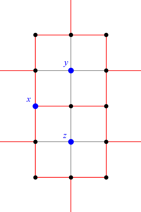
For an illustration of resampling an excursion we refer to Figure 16 and Figure 17. One could ask why one does not choose the index uniformly at random out of the set . The reason for choosing the index out of the set is that by this procedure one guarantees that resampling an excursion does not change the depth profile of the configuration .


For our adapted Glauber dynamics it is important to decide if an edge of a fake local minimum at is in an excursion or not. The next lemma helps a lot in that task.
Lemma 4.19.
Let be a fake local minimum for the homomorphism and let be an edge starting from . The edge is not in an excursion that starts at if and only if there exist an infinite path and such that:
- (1)
For all
- (2)
Moreover, two edges and are in a common excursion of starting at if both edges are in an excursion and there exist a path whose first and last edges are and and such that for all .
Proof of Lemma 4.19.
Suppose that is not in an excursion, and consider the connected component of which contains where is the complete tree with root . By definition is not in an excursion if and only the depth is not bounded from above on . Consider a sequence in such that for all , and build a path that goes through all the ’s while staying in (this is always possible since is connected), then verifies the conditions of the lemma. Reciprocally, if is in an excursion for then the depth is bounded from above on and any path on which the depth is not bounded from above must leave at some point. ∎
The resampling-step will be used in our construction of the adapted Glauber dynamics. It is important to show that resampling maps an element from onto an element in . This is a direct consequence of the following statement.
Lemma 4.20.
Assume that . Then it holds that an edge is in an excursion if an only if for all the edge is also in an excursion. Additionally, it holds that and are on the boundary of a common excursion if and only if for all the edges and are also one the boundary of a common excursion.
Proof of Lemma 4.20.
Both claims follow from the fact that translating by leaves the depth difference invariant since the two-sided geodesic which support the configuration is left unchanged by translation.
Hence, if there exist an infinite path such that for all and . Then the path also verifies for all and .
Similarly two edges and are on the boundary of a common excursion if there exist a path such that for all which is true if and only if the path also verifies for all . ∎
We are now almost ready to define our adapted Glauber dynamics. Before we proceed we need to describe how to go from a Markov chain on to a Markov chain on : A Markov chain on the space induces a Markov chain on using the natural operation of geodesic shift which simply pin at the right place on the geodesic. In the rest of Section 4 we assume wlog. that the geodesic is the only two-sided geodesic going through all the vertices for . Since all geodesics are isomorphic, it is sufficient to prove the concentration inequality (45) for this specific choice of .
Definition 4.21 (geodesic shifts).
Let we define the shift by
| (179) |
Remark 4.22.
An easy way to describe the shift of is to say that it is the only homomorphism in such that .
The geodesic shift leaves the gradient homomorphism associated to an homomorphism invariant. Hence for all since the depth difference between two points is a gradient measurable quantity.
Now, let us describe the adapted Glauber dynamics on that is used in the proof of Lemma 4.10.
Definition 4.23 (Adapted Glauber dynamics).
Let and let be the canonical geodesic path between and defined in (166). Let and denote by the set of homomorphisms such that for . We consider the following dynamics on . Let . Then the new configuration is obtained in the following way:
- (1)
Choose a vertex .
- (2)
If is not fixed then resample all the excursions of that start in . If becomes an extremum, pivot after that and resample again all the excursions of that start in .
- (3)
If is fixed (that is for and ) then only resample all the excursions of that start in but do not pivot .
Remark 4.24.
Since the adapted Glauber dynamics only depends on gradient measurable events and the geodesic shift leaves the gradient invariant, the Markov chain on given by Definition 4.23 induces a Markov chain on the state space of homomorphisms such that
for .
In the next lemma, we show that the adapted Glauber dynamics converges to the correct law once it is projected on .
Lemma 4.25.
Proof of Lemma 4.25.
We start with observing that the adapted Glauber dynamics leaves invariant. Resampling excursions around a vertex does not change the depth of or and the dynamics only pivot vertices whose depth is not fixed.
We now show that the Markov chain is reversible wrt. the uniform probability measure on . Because we consider the uniform probability measure on it suffices to show that
| (180) |
Let denote the position that is chosen in the first step of the adapted Glauber dynamics. We notice that after conditioning on both the law given by resampling an excursion and pivoting are uniform over the spaces of reachable configurations in . Thus we have that
| (181) | ||||
| (182) | ||||
| (183) | ||||
| (184) |
This shows that the projected adapted Glauber dynamics is reversible on the state space .
Now, we prove that the chain is irreducible. To show the irreducibility, one notices that in the first step there is a positive probability that the adapted Glauber dynamics transforms after finitely many steps to a configuration that is entirely supported on the two-sided geodesic and thus the same holds for . Indeed, one can consider a sequence of moves which does not pivot any point but at each step fold one of the excursion of to the geodesic using the excursion resampling. Since a given configuration only have a finite number of excursions, it takes finitely many move for this configuration to be completely folded on using this process.
Now the main idea is the following. In every step, there is a positive probability that the resampling excursions does not change the configuration . Therefore, the Markov chain is irreducible if the original Glauber dynamics is irreducible on the space of configurations which are entirely supported on in . This means that the question of irreducibility of the adapted Glauber dynamics on has been reduced to the question of the original Glauber dynamics being irreducible for graph homomorphisms taking value in , which we show now.
We define the distance between and in that are entirely supported on by
It is clear that implies equal and that must be finite since is finite. Hence, if we show that there exists always a pivot move which decreases the distance between two configurations, we can use inductive argument to prove that the chain is irreducible. Let be the cluster in on which the function is maximal and let be a point in . Suppose without restriction than is greater than on and define to be a maximal increasing path for the depth of starting from . That is a path of maximal length such that for all . This path has to be finite otherwise there exist two points and along the path which are -translates of each other and the slope verifies . All points on the path have to be in since for all :
Moreover, the fact that is of maximal length impose that is a local maximum for the depth. Hence it is possible to do a pivoting move at which decrease the depth of by and decrease the distance between and .
Because the Markov chain has a finite state space and is reversible, it follows from standard theory of Markov processes that the law of the chain converges to the unique invariant probability measure (see for example [Dur10]) on . ∎
Before proceeding to the proof Lemma 4.10 let us provide some auxiliary statements.
Lemma 4.26.
Let such that
| (185) |
Let be a local minimum for both and such that
| (186) |
Then it holds that:
| If an edge is not in an excursion of starting at , | (187) | |||
| then is also not in an excursion of starting at . | (188) |
Additionally, assume that the edges are the same excursion for around . Then it holds that:
| Either all the edges in are in a | (189) | |||
| common excursion for starting at | (190) | |||
| or no edge in is in an excursion for starting at . | (191) |
Proof of Lemma 4.26.
Argument for (187): Let be not in an excursion for that starts in . We know from Lemma 4.19 that there exists an infinite path such that for all . Since and
this also imposes that for all for all . This means that cannot be in an excursion for .
Argument for (189): We show the statement for only two edges and . The generalization to arbitrary many edges is straightforward. It follows from Lemma 4.19 that if two edges and are in the same excursion for then there exists a path such that for all . For the same reason as in the previous paragraph, this imposes that for all . This yields that either and are in the same excursion for or both are not in an excursion for . ∎
The following auxiliary statement is a simple consequence of Lemma 4.26.
Lemma 4.27.
Consider the same hypothesis as in Lemma 4.26. Let be the set of excursions of a graph homomorphism starting at . For each different excursion , choose an edge in starting at to be a representative edge of and denote by the set containing those edges. It follows that is exactly equal to the number of different excursions around for the homomorphism (see Figure 15 for an example) and that
| (192) |
Proof of Lemma 4.27.
Lemma 4.28.
Let such that is a local minimum of . Let denote the state one obtains after the resampling the excursions of and starting at (see Definition 4.18) and let denote the probability that has a true local minimum at . Then:
| (193) |
Here denotes the number of different excursions around for the homomorphism .
Proof of Lemma 4.28.
Let us first consider the case in which all edges around are in an excursion of starting at . The resampling step means that each excursion of starting at will be attached to an uniformly chosen direction that increases the depth (see Definition 4.18 and Figure 16 and Figure 17). Note that in a -regular tree there are many such directions. We recall that denotes the probability that becomes a true local minimum after resampling the excursions starting at (see Definition 4.11). To get a local minimum all excursions must head into the same direction. Hence, for the first excursion one can choose any direction, but all other excursions must head into the same direction, which yields the desired formula
| (194) |
Now, let us consider the second case in which there is an edge around that is not in an excursion of . It follows from the statement (177) that the graph homomorphism heads in the same direction for all the edges around that are not in an excursion. Hence, in order for to become a true local minimum after resampling the excursions around , all the excursions have to head into the same direction. This yields the desired formula
| (195) |
∎
The following auxiliary statement is the main ingredient of the proof of Lemma 4.10.
Lemma 4.29.
Let such that
| (196) |
Let be a local minimum for both and such that
| (197) |
Let denote the state one obtains after resampling the excursions of and starting at (see Definition 4.18). Then it holds that
| (198) |
where and denote the probability that and respectively have a true local minimum at .
Proof of Lemma 4.29.
We verify the desired estimate (198) by considering several cases. In the first case, let us assume that there is an edge around that is not in an excursion for starting at . It follows from the statement (187) that there is also an edge that is not in an excursion for starting at . Hence, it follows from a combination of (192) and (193) that
| (199) |
Let us consider the second case in which all edges starting at for are in an excursion for . We make a further distinction and additionally assume that all the edges starting at are also in an excursion for . In this case, a combination of (192) and (193) yields that
| (200) |
Let us now consider the last case in which we assume that all edges starting at are in an excursion for but there is an edge starting at that is not in in excursion for . In this case it we will show that
| (201) |
Postponing the verification of (201) we get by using (201), (192) and (193) that
| (202) |
which closes the argument.
The only step remaining is to prove (201). Denote by and the set of excursions starting at of and respectively and for each excursion , denote by its representative edge in . As a consequence of the statement (189), we know that the edges must be in different excursions of . Hence, re-indexing allows us to assume that for . Recall that we assumed that there exist an edge that is not in an excursion of . Since by assumption all edges near are in an excursion of it follows that there is an index such that . We will show in a moment that for all
| (203) |
This means that the graph homomorphism has at least many different excursions that start at , which verifies (201).
Let us turn to the verification of (203). We use an indirect argument and assume that wlog.
| (204) |
Hence, the edge and are in the same excursion . By the statement (189) this implies that either or both edges and are not in an excursion. This is a contradiction to the fact that by construction
| (205) |
∎
Now, we are ready to state the proof of Lemma 4.10.
Proof of Lemma 4.10.
We consider a Markov chain on the state space
given by the adapted Glauber dynamics of Definition 4.23. Let
denote the Markov chain on the state space that is also given by the adapted Glauber dynamics of Definition 4.23. As outlined before, the strategy is to define a coupling of those Markov chains such that
| (206) |
We postpone the verification of (206) and show how it is used to derive the statement of Lemma 4.10. We pick arbitrary and set . Then by the Kirszbraun theorem (cf. Theorem 3.9) there exists an element such that
| (207) |
Hence, if we set and we get from (206) that for any realization of the Markov chain and all
| (208) |
The last estimate implies
| (209) |
Now Lemma 4.25 yields that
| (210) |
and
| (211) |
Hence, we overall get the desired estimate (173)
| (212) |
The only thing left to show is that such a coupling indeed exists. Let us consider an element such that
| (213) |
Then every coupling of the chain and works because the adapted Glauber dynamics can only increase the depth deviation in one time step by 2.
Therefore, let us now consider an element such that
| (214) |
W.l.o.g we assume that (else we just interchange the role of and in the argument)
| (215) |
In this situation, if a coupling pivots the same points for the configurations and , there is only one scenario in which the original Glauber dynamics would increases the depth deviation to 4, more precisely, such that
| (216) |
The scenario is when is a true local minimum for and a fake local minimum for (recall that fake local maxima cannot exist for tree-valued height functions, cf. Remark 4.12). The depth deviation could now increase if the Glauber dynamics selects the site . Then the Glauber dynamics could pivot but not , which could possibly increase the depth deviation to 4. However, using the excursion resampling we can show that there is a coupling that prevents this scenario from happening.
Let us explain this strategy in more details. First of all, we want to mention that resampling an excursion does not change the depth of a configuration. Hence, the additional resampling steps of our adapted Glauber dynamics cannot create a violation of the desired conclusion (206). Down below, we construct a coupling such that
| (217) | ||||
| (218) |
where and denote the states obtained after resampling the excursions starting at the vertex for the homomorphisms and respectively. The next step of our Markov chain is pivoting and around . Now, this step can easily be coupled such that if increases or decreases, then so does . This implies the desired conclusion (206).
We explain now how to construct a coupling that satisfies the statement (217). The auxiliary Lemma 4.29 from below states that
| (219) |
where is the probability that is a true minimum of after resampling of the excursions starting at . The quantity is defined analogously. It is a direct consequence of (219) is that there is a coupling of the resampling step such that (217) is satisfied: One throws a random variable that is uniformly distributed on . If one decides that both and will have a true local minimum around , and and are chosen uniformly among those states. If one decides that only will have a true local minimum around , but not . And finally if , one decides that both and will not have a true local minimum around . This completes the argument. ∎
5. Existence of a continuum of shift-invariant ergodic gradient Gibbs measures
This section is independent of the variational principle (cf. Theorem 2.12 and Theorem 2.14) and of its own interest. The Kirszbraun theorem and the concentration estimate obtained in Section 4 carry important information about the set of gradient Gibbs measures that are ergodic wrt. the translations of . In this section, we show the existence of a continuum of translation-invariant, ergodic, gradient Gibbs measures. In order to make our statement precise, we begin with recalling some classical results about Gibbs measures for discrete systems. They can all be found in [Geo88].
Definition 5.1 (Slope).
Let be a gradient Gibbs measure that is ergodic wrt. translations of . Then for all the limit
exists -almost surely and we call the slope of .
It is a classical result (e.g [Cha16]) that the subadditive ergodic theorem implies the existence of this limit. Moreover, every translation invariant gradient Gibbs measure can be decomposed into a mixture of ergodic gradient Gibbs measures. The latter allows to define the slope of a translation invariant Gibbs measure in the following way:
Definition 5.2.
Let be a translation invariant gradient Gibbs measure. Then the slope of is
where is the ergodic decomposition of . This means that for any test function it holds that
| (220) |
We will now show how the concentration inequality of Theorem 3.10 implies the existence of an ergodic gradient Gibbs measure for each slope whose -norm is strictly less than . Before we are able to prove the main theorem of this section we provide some auxiliary statements.
Lemma 5.3.
Let be such that . Then there exists a sequence of -translation invariant homomorphisms with slope (cf. Definition 3.2).
Proof.
The proof is a direct consequence of the Kirszbraun theorem. Let be a two-sided geodesic. For all , set . Since is isomorphic to we can apply the Kirszbraun theorem between and . Hence, there exist an extension of on the whole space which is entirely supported on the geodesic . The slope of this extension must be which concludes our proof. ∎
Lemma 5.4.
Let be such that and let be small enough. Then there exist universal constants and independent of such that for all
| (221) |
Proof.
Wlog. we assume that . We start with deducing the auxiliary estimate
| (222) |
for some universal constants .
Indeed, let us recall the concentration inequality from Lemma 4.7
| (223) |
and also that (see the proof of Theorem 3.10)
By combining the two previous observations and summing over all possible such that we obtain that
| (224) | ||||
| (225) |
Let us now bound the probability that is far from the geodesic . Suppose that for
Recall by convention of the set that or . Walking along the -axis, we denote by the first integer such that or . Notice that we must necessarily have . Moreover, by convention we have . Therefore, we get
Let us now turn to the verification of (221). Using the triangle inequality yields that
Hence
| (227) | |||||
since for the left-hand event to happen one of the two right-hand events must happen. Using (224) and (222) together this implies that
for some universal constants independent of . This completes the argument. ∎
Let us now prove the existence of a continuum of ergodic gradient Gibbs measures.
Theorem 5.5.
For all such that , there exists an ergodic gradient Gibbs measure with slope .
Proof of Theorem 5.5.
We already know from the previous lemma that for all the set is non empty. Hence, the uniform probability measure on exists. By compactness of the space of gradient Gibbs measures in the topology of local convergence, we can extract a subsequence which converges to a gradient Gibbs measure on the infinite volume space (see Lemma 8.2.7 of [She05] for more details). The shift invariance of the measure follows from the shift invariance of the spaces . This means that we can write the measure as a mixture of ergodic Gibbs measures (see Definition 5.2). Suppose, by contradiction that the slope is not almost surely equal to on the average . Then there exist , and such that , wlog. we will assume that . Applying Lemma 5.4 we obtain that there exist universal constants and independent of such that:
| (228) |
Dividing by we can rewrite this inequality as
Thus, by going to the subsequential limit first in and then in it holds that
On the other hand, we have that
| (229) | ||||
| (230) | ||||
| (231) | ||||
| (232) | ||||
| (233) |
which is a contradiction. Therefore, the slope is -almost surely equal to and there exists at least one ergodic gradient Gibbs measure with slope . ∎
6. Proof of the variational principle
In this section we prove the results of Section 2. More precisely, we give the proof of Lemma 2.8, Theorem 2.12 and Theorem 2.14. We start with the proof of Lemma 2.8. The argument uses a standard construction to extend Lipschitz functions from the boundary to the whole set .
Proof of Lemma 2.8.
Let be an asymptotic boundary height profile on and define by:
| (234) | ||||
| (235) |
We will show that extends to an asymptotic height profile on the whole region . In order to prove this we show the following three properties:
The first property is a simple consequence of the inequality (9) that holds for the function . Indeed using (9) yields that for all we have and thus .
For the second property, we first observe that by a combination of the triangle inequality and the fact that satisfies (9) on , the function given by
satisfies on the condition (9). It is now a simple consequence that also satisfies (9) on .
Let us turn to the third property. We show the third property by contradiction. Let us assume that the map does not satisfy the condition (10). Then there is a point such that
| (236) |
Then by continuity there are two points such that
| (237) |
By definition (234) of the map it follows that there is a point and such that
| (238) |
and
| (239) |
Because we can choose to be arbitrarily small the last estimate yields that
| (240) |
A combination of (238) and(240) yields that
| (241) | ||||
| (242) |
The last estimate contradicts inequality (14) and completes the argument. ∎
Let us turn to the verification of Theorem 2.12 and Theorem 2.14. For the general strategy of the argument we refer to the discussion at the end of Section 2. First, we turn to the proof of Theorem 2.14. As explained at the end of Section 2 the main ingredient is to show the equivalence of the entropy of fixed and fluctuating boundary conditions on a simplex. This ingredient is provided in Lemma 6.3 below. Before turning to Lemma 6.3, we show in the next auxiliary lemma that if the boundary height function on a simplex is close to an affine function then it must stay close to a single geodesic. Similar to Remark 2.15 of Section 2, this also justifies that the entropic effect, that results from the additional freedom of choosing the geodesic , is of lower order.
Definition 6.1.
A geodesic segment is given by an injective graph homomorphism (cf. Definition 2.4).
Lemma 6.2.
We consider the simplex
Let , let and let such that . Let be a graph homomorphism such that for all :
| (243) |
Then there exist a geodesic segment such that for all :
| (244) |
where denotes the unique element such that
Proof of Lemma 6.2.
We start by proving the following auxiliary statement: Let be a graph homomorphism satisfying the conditions of Lemma 6.2. If is a path in on which the function is non-decreasing then there exist a geodesic segment such that for all :
| (245) |
Argument for (245): Let denote the geodesic segment of between the vertices and . We then define to be a geodesic segment which goes through the root , the vertex with lowest depth in and . This construction insure that the depth is strictly increasing along . We suppose that there exist such that
By definition of a geodesic segment in a tree, the path has to return to . Let denote the smallest number such that . Then it holds that . A direct calculation yields (cf. the proof of Theorem 3.10) that
| (246) | ||||
| (247) | ||||
| (248) | ||||
| (249) |
Hence, it follows that either
or
which is a contradiction with our starting hypothesis and completes the proof of (245).
Let us now turn to the main argument. We distinguish the cases and .
If then for all the sets are connected as subsets of the graph . As a consequence we obtain that is also a connected subset of the tree . Thus for all :
| (250) |
Moreover, both the maximum and the minimum of the function on must be reached on some corner (non-necessarily unique) of the simplex . Consider two such corners and which reach respectively the minimum and the maximum of and define to be an increasing path on between and . We can use (245) to define a geodesic segment such that for all :
| (251) |
Since each vertex in is in for some , we must have that for all . This concludes our proof for .
Let us now consider the case . The reasoning is similar, there must be two extremal vertices and of the simplex which minimize and maximize the function on . Moreover both geodesic paths from to are necessarily increasing for the function
Hence we obtain that for all :
| (252) |
where is a geodesic segment defined as in the first part of this proof. ∎
We will now show that the entropy per site on a simplex for fluctuating linear boundary conditions is equivalent to the local surface tension as .
Lemma 6.3.
Remark 6.4.
Since the volume of the simplex is , the quantity can be understood as the entropy per site associated to fluctuating boundary conditions on with slope .
We already deduced an analogous result for hypercubes in Theorem 3.12. Hence, the main idea of the proof of Lemma 6.3 consists of leveraging the result of Lemma 6.3 to simplices by a two-scale decomposition of a simplex into smaller cubes, and vice versa.
Proof of Lemma 6.3.
Let . By Lemma 6.2, there exist a geodesic segment such that for all :
| (255) |
We start with showing that the entropic effect of having different geodesic segments is negligible. Therefore, let us estimate how many different geodesic segment can exist. On there are less than possible distinct boundary graph homomorphisms. Hence, the number of possible distinct geodesic segments is also bounded by , which is of lower order.
As a consequence let us fix a geodesic segment . It is sufficient to show that for all such that
| (256) |
the number of homomorphisms which extends the boundary height function to the whole verifies
| (257) |
Indeed, since the number of different homomorphisms restricted to is bounded by , this directly implies the desired statement of Lemma 6.3.
In order to deduce the estimate (257) we consider the cases and separately.
In the case we observe that by definition . Hence, the verification of (257) is reduced to a straightforward combinatorial argument using Stirling formula which is left out in this article (see e.g [CKP01] Lemma 3.5 or [MPT18] Lemma 5.1 for an analogous argument).
Argument for (258): The argument consists of dividing a large simplex in smaller cubes. We underestimate the entropy (i.e. overestimate the number of configurations) by choosing independent periodic boundary conditions on each cube. This will yield the correct lower bound by Theorem 3.12. Let us now give the details of the argument. Consider an dimensional hypercube with edge size and lower left corner at the origin. We use now the convention that
where is the restriction of to the boundary . This means that is the periodic boundary data of slope on which has the most possible extensions to a graph homomorphism on among all periodic boundary data of slope on .
By definition of , it follows that is bounded by times the number of possible boundary homomorphisms on . More precisely,
Now we fix small enough and define for the translated hypercube
Let us consider the subset of
The set indexes all hypercubes that are contained in the simplex and not too close to the boundary (cf. the right side of Figure 18). The cardinality of all sites contained in those boxes (represented in light grey in the right side of Figure 18) is bounded from below by
Here, the second term of the bound comes from the maximum number of cubes that are removed from the strip of size along the border of the simplex. Moreover, since the boundary homomorphism is -periodic, there exist a graph homomorphism
such that for all :
Here, and are the gradient graph homomorphisms associated to and respectively, and is the shift by in . Using Lemma 6.2, we observe that there exist a one sided geodesic such that
We choose wlog. to be the same geodesic for both and .
As a consequence, it is possible for to extend the homomorphisms to on (use a similar calculation as in equation (54) of Lemma 3.11 and the Kirszbraun theorem for graphs). If we combine the previous observations we obtain that:
| (260) | |||||
| (261) | |||||
| (262) |
Sending now first and then yields the desired estimate (258).
Argument for (259): Let us describe the main strategy. We will overestimate the entropy on a cube by underestimating the possible number of configurations. We observe that on the continuum there is a natural decomposition of a cube into simplices. We now leverage this decomposition onto the lattice, fitting simplices of size in a cube of size slightly larger than . We now underestimate the number of configurations by fixing the boundary values on each simplex. Because we leave enough space between the simplices, we can glue together the boundary graph homomorphisms by the Kirszbraun theorem. Now, the entropy per site on each simplex is an upper bound for the entropy per site on the large cube yielding the correct estimate by Theorem 3.12.
Let us now outline the details of the construction. We can tile the hypercube of size using simplices of size each within distance of each other (see the left side of the Figure 18). Let us now explain how to choose the boundary condition on each simplex. The boundary condition will be fixed by a graph-homomorphism . Let be a graph-homomorphism such that
| (263) |
We observe that the all simplices in the cube are characterized by -permutations . For a given permutation we define as the simplex obtained by permuting the coordinates of according to . Let us denote by the graph-homomorphisms on obtained by permuting the coordinates components of according to . We set on the boundary of each one of those simplices. Moreover, by the Kirszbraun theorem (see also equation (54) of Lemma 3.11) we can extend the homomorphism to . Now, we underestimate the number of graph homomorphisms in by
| (264) | ||||
| (265) | ||||
| (266) |
By self-similarity of the simplices this implies that
| (267) |
and therefore
| (268) |
which verifies (259).∎

In the proof of Theorem 2.14 we use the observation that -Lipschitz functions can be approximated very well by affine functions on a simplicial complex.
Definition 6.5.
We denote by the simplicial lattice of formed by the points on the boundary of the simplices
for any -permutation and . Let denote a function on such that is piecewise affine on the simplicial lattice and for all vertices of the simplicial lattice . The function is called affine approximation of .
Remark 6.6.
Using our previous notation in Definition 2.13 we have that .
Lemma 6.7 (Approximation via triangulation).
Let be an affine approximation of as defined above. For let be the union of all simplices strictly included in and such that:
.
Then it holds that for sufficiently small
- (1)
,
- (2)
.
The statement of Lemma 6.7 is proven in the two dimensional case in Lemma 2.2 and Lemma 2.3 of [CKP01]. The proof does not involve any argument specific to the -dimensional case and can be naturally generalized to -dimensional simplices. Hence we are not reproving Lemma 6.7 in this article. Let us now turn to the proof of Theorem 2.14.
Proof of Theorem 2.14.
Recall the definition of the sets
| (269) | ||||
| (270) |
For and , denote . For fixed and given the asymptotic height profile let us consider the affine approximation of on the simplicial lattice (see Definition 6.5). It follows from Lemma 6.7 that
Hence, Theorem 2.14 is a consequence of the following statement:
| (271) |
We also know from property (1) of Lemma 6.7 that
Let us now start by underestimating the number of homomorphisms in . We begin by proving that is non-empty for large enough. Define to be the graph homomorphism such that for all :
According to the definition of the convergence of a sequence of boundary height functions, for large enough the following holds:
Hence we can apply Corollary 4.4 to the homomorphism and any graph homomorphism which extends on to deduce that there exist at least one homomorphism (depending on ) defined on in .
For a given simplex with , denote by the same simplex scaled by and belonging to . It follows directly from the definition of that for all simplex :
As a consequence for all , the homomorphism is in .
We can now underestimate the number of homomorphisms in by counting all configurations exactly equal to on the boundary of the simplices such that . This gives us:
| (272) | |||||
| (273) | |||||
| (274) | |||||
| (275) |
where in the third inequality we used Lemma 6.3 and in the last inequality we used that by definition
Let us now turn to the overestimation of the number of graph homomorphisms in . Any function which is within of on must be within of on . Hence, the strategy is to look at the free product of all configurations such that stays within of on each rescaled simplex for which . We subsequently multiply this number by which is a natural upper bound on the number of different configurations outside of those simplices. This gives an upper bound on the total of possible homomorphisms in . Using the same notations as in Lemma 6.3, we obtain:
| (276) | ||||
| (277) | ||||
| (278) | ||||
| (279) | ||||
| (280) | ||||
We deduce Theorem 2.12 from Theorem 2.14 using a compactness argument similar to the one used in [CKP01].
Proof of Theorem 2.12.
For a fixed asymptotic boundary height profile let us consider the set of all possible extensions to an asymptotic height profile (see Definition 2.3). We observe that
We observe that the space is closed and that the local surface tension is convex (cf. Theorem 3.15) and uniformly bounded from below by . Hence, it follows that
| (281) | ||||
| (282) |
where is a minimizer of the macroscopic entropy .
Let us fix an . We have to show that there exists an integer such that for all it holds
| (283) |
and
| (284) |
We start with deducing the estimate (283). Underestimating the number of graph homomorphisms and using the identity (28) of Theorem 2.14 yields that
| (285) | ||||
| (286) | ||||
| (287) |
Choosing now first small then small (depending on ), and finally large (depending on and ) yields the desired upper bound (283).
Let us now deduce the lower bound (284). This is equivalent to showing that for all :
| (288) |
Choose , we know from (28) that all asymptotic profile there exist (depending on and ) and (depending on , and ) such that
| (290) |
Since the set of -Lipschitz functions defined on a closed bounded region is compact, there exist an integer , depending on but not on , and a collection of asymptotic height profiles such that
| (291) |
By taking the logarithm and using the identity (28) of Theorem 2.14 we obtain that
| (292) | ||||
| (293) | ||||
| (294) | ||||
| (295) |
which finishes the proof. ∎
Acknowledgement
The authors want to thank Marek Biskup, Nishant Chandgotia, Filippo Colomo, Nicolas Destainville, Richard Kenyon, Michel Ledoux, Igor Pak, Laurent Saloff-Coste, Scott Sheffield, Peter Winkler and Tianyi Zheng for helpful discussions and comments. The authors also would like to express special thanks of gratitude to the anonymous referees and to Andrew Krieger. Their precise comments and questions helped a lot to further improve the manuscript.
References
- [Azu67] Kazuoki Azuma. Weighted sums of certain dependent random variables. Tôhoku Math. J. (2), 19:357–367, 1967.
- [BCG16] Alexei Borodin, Ivan Corwin, and Vadim Gorin. Stochastic six-vertex model. Duke Math. J., 165(3):563–624, 02 2016.
- [BW00] Graham R. Brightwell and Peter Winkler. Gibbs measures and dismantlable graphs. J. Combin. Theory Ser. B, 78(1):141–166, 2000.
- [CEP96] Henry Cohn, Noam Elkies, and James Propp. Local statistics for random domino tilings of the Aztec diamond. Duke Math. J., 85(1):117–166, 1996.
- [Cer06] R. Cerf. The Wulff crystal in Ising and percolation models, volume 1878 of Lecture Notes in Mathematics. Springer-Verlag, Berlin, 2006. Lectures from the 34th Summer School on Probability Theory held in Saint-Flour, July 6–24, 2004, With a foreword by Jean Picard.
- [Cha16] Nishant Chandgotia. Four-cycle free graphs, height functions, the pivot property and entropy minimality. Ergodic Theory and Dynamical Systems, FirstView:1–31, 3 2016.
- [CKP01] Henry Cohn, Richard Kenyon, and James Propp. A variational principle for domino tilings. J. Amer. Math. Soc., 14(2):297–346 (electronic), 2001.
- [CPST18] Nishant Chandgotia, Ron Peled, Scott Sheffield, and Martin Tassy. Delocalization of uniform graph homomorphisms from to , 10 2018.
- [CS16] F. Colomo and A. Sportiello. Arctic curves of the six-vertex model on generic domains: The tangent method. Journal of Statistical Physics, 164(6):1488–1523, 2016.
- [DCPSS17] Hugo Duminil-Copin, Ron Peled, Wojciech Samotij, and Yinon Spinka. Exponential decay of loop lengths in the loop o (n) model with large n. Communications in Mathematical Physics, 349(3):777–817, 2017.
- [Des98] N. Destainville. Entropy and boundary conditions in random rhombus tilings. J. Phys. A, 31(29):6123–6139, 1998.
- [DKS92] R. Dobrushin, R. Kotecký, and S. Shlosman. Wulff construction, volume 104 of Translations of Mathematical Monographs. American Mathematical Society, Providence, RI, 1992. A global shape from local interaction, Translated from the Russian by the authors.
- [Dur10] Rick Durrett. Probability: theory and examples. Cambridge Series in Statistical and Probabilistic Mathematics. Cambridge University Press, Cambridge, fourth edition, 2010.
- [FS97] T. Funaki and H. Spohn. Motion by mean curvature from the ginzburg-landau interface model. Communications in Mathematical Physics, 185(1):1–36, Apr 1997.
- [FS06] Patrik L. Ferrari and Herbert Spohn. Scaling limit for the space-time covariance of the stationary totally asymmetric simple exclusion process. Comm. Math. Phys., 265(1):1–44, 2006.
- [Geo88] Hans-Otto Georgii. Gibbs measures and phase transitions, volume 9 of de Gruyter Studies in Mathematics. Walter de Gruyter & Co., Berlin, 1988.
- [Hoe63] Wassily Hoeffding. Probability inequalities for sums of bounded random variables. J. Amer. Statist. Assoc., 58:13–30, 1963.
- [Kas63] P. W. Kasteleyn. Dimer statistics and phase transitions. J. Mathematical Phys., 4:287–293, 1963.
- [Kir34] M. Kirszbraun. Über die zusammenziehende und Lipschitzsche Transformationen. Fundamenta Mathematicae, 22(1):77–108, 1934.
- [KK92] Claire Kenyon and Richard Kenyon. Tiling a polygon with rectangles. In Foundations of Computer Science, 1992. Proceedings., 33rd Annual Symposium on, pages 610–619. IEEE, 1992.
- [Klo08] Benoît Kloeckner. On Lipschitz compactifications of trees. Comptes Rendus Mathematique, 346(7):413 – 416, 2008.
- [KO+07] Richard Kenyon, Andrei Okounkov, et al. Limit shapes and the complex burgers equation. Acta mathematica, 199(2):263–302, 2007.
- [KS99] Michael K.-H. Kiessling and Herbert Spohn. A note on the eigenvalue density of random matrices. Communications in Mathematical Physics, 199(3):683–695, Jan 1999.
- [LP08] Lionel Levine and Yuval Peres. Strong spherical asymptotics for rotor-router aggregation and the divisible sandpile. Potential Analysis, 30(1):1, 2008.
- [LRS01] Michael Luby, Dana Randall, and Alistair Sinclair. Markov chain algorithms for planar lattice structures. SIAM J. Comput., 31(1):167–192, 2001.
- [LS77] B. F. Logan and L. A. Shepp. A variational problem for random Young tableaux. Advances in Math., 26(2):206–222, 1977.
- [MKT17] Georg Menz, Andrew Krieger, and Martin Tassy. A quenched variational principle for discrete random maps. arXiv:1710.11330, 2017.
- [MPT18] Alejandro Morales, Igor Pak, and Martin Tassy. Asymptotics for the number of standard tableaux of skew shape and for weighted lozenge tilings. arXiv preprint arXiv:1805.00992, 2018.
- [NR16] Ananth Sridhar Nicolai Reshetikhin. Limit shapes of the stochastic six vertex model. arXiv:1609.01756, 2016.
- [PR07] Boris Pittel and Dan Romik. Limit shapes for random square Young tableaux. Adv. in Appl. Math., 38(2):164–209, 2007.
- [PST16] Igor Pak, Adam Sheffer, and Martin Tassy. Fast domino tileability. Discrete Comput Geom, 56(2):377–394, 2016.
- [Sch69] J. T. Schwartz. Nonlinear functional analysis. Gordon and Breach Science Publishers, New York-London-Paris, 1969. Notes by H. Fattorini, R. Nirenberg and H. Porta, with an additional chapter by Hermann Karcher, Notes on Mathematics and its Applications.
- [She02] Scott Sheffield. Ribbon tilings and multidimensional height functions. Transactions of the American Mathematical Society, 354(12):4789–4813, 2002.
- [She05] Scott Sheffield. Random surfaces. Astérisque, (304):vi+175, 2005.
- [Tas14] Martin Tassy. Translation invariant Gibbs measure on tilings. In preparation, Brown University, 2014.
- [Val43] F. A. Valentine. On the extension of a vector function so as to preserve a Lipschitz condition. Bull. Amer. Math. Soc., 49:100–108, 1943.
- [vB77] Henk van Beijeren. Exactly solvable model for the roughening transition of a crystal surface. Physical Review Letters, 38, 05 1977.
- [VK77] A. M. Veršik and S. V. Kerov. Asymptotic behavior of the Plancherel measure of the symmetric group and the limit form of Young tableaux. Dokl. Akad. Nauk SSSR, 233(6):1024–1027, 1977.
- [Wig59] E. Wigner. Statistical properties of real symmetric matrices with many dimensions. In 4th Can. Math. Congress (Banff 1957), page 174–184. Univ. Toronto Press, 1959.
- [Wil04] David Bruce Wilson. Mixing times of lozenge tiling and card shuffling Markov chains. Ann. Appl. Probab., 14(1):274–325, 02 2004.