Mean trapping time for an arbitrary node on regular hyperbranched polymers

Junhao Peng Affiliation: 1.School of Math and Information Science, Guangzhou University, Guangzhou 510006, China. Affiliation: 2.Key Laboratory of Mathematics and Interdisciplinary Sciences of Guangdong Higher Education Institutes, Guangzhou University, Guangzhou 510006, China. Email: pengjh@gzhu.edu.cn Email:

Abstract

The regular hyperbranched polymers (RHPs), also known as Vicsek fractals, are an important family of hyperbranched structures which have attracted a wide spread attention during the past several years. In this paper, we study the first-passage properties for random walks on the RHPs. Firstly, we propose a way to label all the different nodes of the RHPs and derive exact formulas to calculate the mean first-passage time (MFPT) between any two nodes and the mean trapping time (MTT) for any trap node. Then, we compare the trapping efficiency between any two nodes of the RHPs by using the MTT as the measures of trapping efficiency. We find that the central node of the RHPs is the best trapping site and the nodes which are the farthest nodes from the central node are the worst trapping sites. Furthermore, we find that the maximum of the MTT is about $4$ times more than the minimum of the MTT. The result is similar to the results in the recursive fractal scale-free trees and T-fractal, but it is quite different from that in the recursive non-fractal scale-free trees. These results can help understanding the influences of the topological properties and trap location on the trapping efficiency.

1 Introduction

In the last few decades, polymer physics has attracted considerable attention within the scientific community, with various polymer networks proposed to describe the structures of macromolecules [1]. Among numerous polymer networks, the regular hyperbranched polymers (RHPs), also known as Vicsek fractals, are important models of the Hyperbranched polymers [2], which have widely applications in coatings [3, 4], conjugated functional materials [5, 6], modifiers and additives [7], drug and gene delivery [8, 9, 10] etc.

In view of the widely applications of the Vicsek fractals, interest in Vicsek fractals is growing rapidly. Jayanthi and Wu [11, 12, 13] succeeded in determining the eigenvalues of connectivity matrix A of the original Vicsek fractals by determining the roots of iteratively constructed polynomials. Blumen et al. [15, 14] determined the eigenvalue spectrum of general Vicsek fractals for any generation $t$ through an algebraic iterative procedure. From these works, one can determine the eigenvalue spectrum of very large Vicsek fractals to very high accuracy, and then calculate many other dynamical quantities of them [16, 17, 18, 19, 20].

Among a plethora of fundamental dynamical processes, random walks are crucial to a lot of branches of sciences and engineering and have appealed much interest [21, 22, 23, 24, 25, 26, 27, 28]. A large variety of other dynamical processes occurring in complex systems can be analyzed and understood in terms of random walks. Examples of these dynamics include energy or exciton transport in polymer systems [29], reaction kinetics [30], and so on. A basic quantity relevant to random walks is the mean first-passage time (MFPT) $F(x,y)$ , which represents the expected number of steps for a walker starting from the source node $x$ to arrive the trap node $y$ for the first time. One can also define the mean trapping time (MTT) for trap node $y$ by

T_{y}=\frac{1}{N-1}\sum_{x\in\Omega,x\neq y}F(x,y),

(1)

where $\Omega$ denotes the node set and $N$ is the total number of nodes.

As is well known, the topological properties of complex system have nontrivial influences on the MTT. Therefore, considerable endeavor has been devoted to uncover the MTT for different topological structures [31, 32, 33, 34, 35, 36, 37, 38, 39, 40, 41, 42, 43]. It is also well known that the trap location has great effect on the MTT and the MTT can be used as the measure of trapping efficiency for different trap node. One should analyze the MTT for an arbitrary trap node and compare the trapping efficiency among all the different traps. The locations which have the minimum MTT can be looked as the best trapping sites and the locations which have the maximum MTT can be looked as the the worst trapping sites. These results have widely application in physical and chemical societies. For example, the best trap sites can be used as the best data collection sites for energy or exciton transport in polymer [29] and geometry-controlled kinetics [30].

In order to analyze the MTT to an arbitrary trap node, one must propose a way to label all the different nodes and then derive formulas to calculate the MTT for the different nodes. For the Cayley trees, Zhang [44] labeled the nodes by its levels and derived the exact analytic formula of the MTT for an arbitrary trap node. For the recursive fractal scale free trees, non-fractal scale-free trees and T-fractal, we labeled its nodes through its edge replacing structure(i.e. the network of generation $k$ , which is denoted by $G(k)$ , is obtained by replacing every edge of $G(k-1)$ by a special structure) [45, 47, 46]. Results shows that the ratio between the maximum and minimum of the MTT is almost a constant in the recursive fractal scale-free trees and T-fractal, whereas it grows logarithmically with network order in the recursive non-fractal scale-free trees. Therefore the effect of trap location on the MTT varies with the topological structures of the complex systems.

As for the Vicsek fractals, they have self-similar treelike structure which can be constructed iteratively by node replacing (i.e. the Vicsek fractals of generation $k$ , which is denoted by $G(k)$ , is obtained by replacing every node of $G(k-1)$ with a star) [48, 15]. The exact analytical solution of the MTT for the central node was obtained in Ref. [49], the exact analytical solution of the MTT for the peripheral node and the global mean first-passage time (i.e., the average of MFPTs over all pairs of nodes) were obtained in Ref. [44], but the MTT for any trap node are still unresolved and one cannot completely uncover the effect of trap location on the MTT in the RHPs.

Although we have proposed method to derived the exact analytic formula of the MTT for an arbitrary trap node in the recursive fractal scale-free trees and the recursive non-fractal scale-free trees [45, 47], the method works good on the iterative structures obtained by edge replacing such as the recursive fractal and non-fractal scale-free trees, tree like fractal, (u, v) flower, etc, it does not work on the iterative structures obtained by node replacing such as Vicsek fractals.

In this paper, we first propose a new way to label all the different nodes of the RHPs and derive exact formulas to calculate the MTT for any node. Then, we compare the trapping efficiency between any two nodes of the RHPs and find the best and worst trapping sites by using the MTT as the measures of trapping efficiency. Our results show that the central node of the RHPs is the best trapping site and the nodes which are the farthest nodes from the the central node are the worst trapping sites. Finally, we find that the maximum of the MTT is almost $\frac{3m^{2}+3m-2}{2m}$ times the minimum of the MTT. The result is similar to the result in the recursive fractal scale-free trees and T-fractal, but it is quite different from that in the recursive non-fractal scale-free trees. These results can help understanding the influences of the topological properties and trap location on the trapping efficiency.

2 The network model

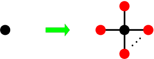
The regular hyperbranched polymers (or Vicsek fractals) [48, 14, 15] of generation $t$ , denoted by $G(t)$ ( $t\geq 0$ ), are constructed in the following iterative way. For $t=0$ , $G(0)$ consists of an isolated node without any edge. For $t=1$ , $m$ $(m\geq 2)$ new nodes are generated with each being connected to the node of $G(0)$ to form $G(1)$ , which is exactly a star. For $t\geq 2$ , $G(t)$ is obtained from $G(t-1)$ . The detailed process is as follow. We introduce $m$ new identical copies of $G(t-1)$ and arrange them around the periphery of the original $G(t-1)$ , and add $m$ new edges, each of them connecting a peripheral node in one of the $m$ corner copy structures and a peripheral node of the original central structure, where a peripheral node is a node farthest from the central node. The first three generations of the Vicsek fractals for the case $m=4$ are shown in figure 1. The Vicsek fractals $G(t)$ can also be constructed by another method, i.e., $G(t)$ is obtained from $G(t-1)$ by replacing every node of $G(t-1)$ with a star as shown in figure 2.

According to its construction, at each generation the total number of the nodes increases by a factor $m+1$ ; therefore, the total number of nodes of $G(t)$ is $N_{t}=(m+1)^{t}$ , and the total number of edges of $G(t)$ is $E_{t}=N_{t}-1=(m+1)^{t}-1$ .

Refer to caption — Figure 1: The first three generations of the Vicsek fractals for the case $m=4$ .

3 The MTT for random walks on Vicsek fractals

3.1 Simplification of the expressions for the MTT

For any two nodes $x$ and $y$ of Vicsek fractals $G(t)$ , $F(x,y)$ is the MFPT from $x$ to $y$ , the sum

k(x,y)=F(x,y)+F(y,x)

is called the commute time and the MFPT can be expressed in term of commute times [50]:

F(x,y)\!=\!\frac{1}{2}\!\left\{\!k(x,y)\!+\!\!\sum_{u\in G(t)}\!\pi(u)[k(y,u)-k(x,u)]\!\right\}\!,

(2)

where “ $u\in G(t)$ ”means that $u$ belongs to the nodes set of $G(t)$ , $\pi(u)=\frac{d_{u}}{2E_{t}}$ is the stationary distribution for random walks on Vicsek fractals and $d_{u}$ is the degree of node $u$ .

If we view the networks under consideration as electrical networks by considering each edge to be a unit resistor and let $\Psi_{xy}$ denote the effective resistance between two nodes $x$ and $y$ in the electrical networks, we have [50]

k(x,y)=2E_{t}\Psi_{xy},

(3)

where $E_{t}$ is the total numbers of edges of $G(t)$ . Since the Vicsek fractals we study are trees, the effective resistance between any two nodes is just the shortest-path length between the two nodes. Hence

\Psi_{xy}=L_{xy},

(4)

where $L_{xy}$ denote the shortest path length between node $x$ to node $y$ . Thus

k(x,y)=2E_{t}L_{xy}.

(5)

Replacing $k(x,y)$ from Eq. (5) in Eq. (2), and defining

S_{x}=\sum_{y\in G(t)}{L_{xy}},

(6)

W_{x}=\sum_{u\in G(t)}\pi(u)L_{xu}=\frac{1}{2E_{t}}\cdot\sum_{u\in G(t)}{(L_{xu}\cdot d_{u})},

(7)

\Sigma=\sum_{u\in G(t)}\left(\pi(u)\sum_{x\in G(t)}L_{xu}\right),

(8)

we obtain

\displaystyle F(x,y)

\displaystyle=

\displaystyle E_{t}(L_{xy}+W_{y}-W_{x}).

(9)

Substituting $F(x,y)$ from Eq. (9) in Eqs. (1), one gets

\displaystyle T_{y}

\displaystyle=

\displaystyle S_{y}+N_{t}\cdot W_{y}-\Sigma.

(10)

Hence, if we can calculate $\Sigma$ and $S_{y},W_{y}$ for any node $y$ , we can calculate $F(x,y)$ for any two nodes $(x,y)$ and the MTT for any node $y$ . In this paper, we calculate these quantities of the RHPs based on its self-similar structure.

3.2 General methods of calculating the MTT

According to the construction of Vicsek fractals, $G(t)$ is composed of $m+1$ copies, called subunit, of $G(t-1)$ which are connected with each other by their peripheral nodes. For convenience, we classify the subunits of $G(t)$ into different levels and let $\Lambda_{k}$ denote the subunit of level $k$ $(k\geq 0)$ . In this paper, $G(t)$ is said to be subunit of level $0$ . For any $k\geq 0$ , the $m+1$ subunits of $\Lambda_{k}$ are said to be subunits of level $k+1$ . Thus, any node of $G(t)$ is a subunit of level $t$ and $\Lambda_{k}$ is a copy of Vicsek fractals with generation $t-k$ . Similarity, we classify all the nodes of $G(t)$ into different levels and the node which is the central node of certain subunit $\Lambda_{k}$ $(k\geq 0)$ is said to belong to level $k$ . The reason for we only assign level $k$ to the central node of subunit $\Lambda_{k}$ is we can use the same labels to label the subunit $\Lambda_{k}$ and its central node.

In order to distinguish the subunits of different locations, inspired by the method of Ref [34], we label the subunit $\Lambda_{k}$ $(0\leq k\leq t)$ by a sequence $\{0,i_{1},i_{2},...,i_{k}\}$ and denote it by $\Gamma_{0,i_{1},i_{2},...,i_{k}}$ , where $i_{j}=0,1,2,\cdots,m$ $(1\leq j\leq k)$ labels its location in its parent subunit $\Gamma_{0,i_{1},i_{2},...,i_{k-1}}$ . In particular, ‘ $\{0\}$ ’represents the Vicsek fractals $G(t)$ itself. figure 3 shows the construction of $\Gamma_{0,i_{1},i_{2},...,i_{k-1}}$ and the way we label its subunits. As shown in figure 3, $\Gamma_{0,i_{1},i_{2},...,i_{k-1}}$ $(k>0)$ , which is represented by the biggest dashed circle, is composed of $m+1$ subunits $\Gamma_{0,i_{1},i_{2},...,i_{k}}$ ( $i_{k}=0,1,2,...,m$ ) represented by solid circles. It also connects with other part of $G(t)$ (i.e., $SG^{i_{k}}_{0,i_{1},\cdots,i_{k-1}},i_{k}=1,2,...,m$ ) at its $m$ corners. Each subunit $\Gamma_{0,i_{1},i_{2},...,i_{k}}$ is also composed of $m+1$ subunits $\Gamma_{0,i_{1},i_{2},...,i_{k+1}}$ represented by small dashed circles. We label the subunit at the center of $\Gamma_{0,i_{1},i_{2},...,i_{k-1}}$ by $i_{k}=0$ and the $m$ peripheral subunits surround the cental one by $i_{k}=1,2,\cdots,m$ . The value of $i_{k}$ shows the relation between $i_{k}$ and the location of subunit $\Gamma_{0,i_{1},i_{2},...,i_{k}}$ in subunit $\Gamma_{0,i_{1},i_{2},...,i_{k-1}}$ . The numbers in each small dashed circles, which are the corresponding values of $i_{k+1}$ , show the relation between $i_{k+1}$ and the location of subunit $\Gamma_{0,i_{1},i_{2},...,i_{k+1}}$ in $\Gamma_{0,i_{1},i_{2},...,i_{k}}$ and $\Gamma_{0,i_{1},i_{2},...,i_{k-1}}$ . But there are two numbers in the two small dashed circles for $i_{k}=1$ . it means the way to label the two subunits of $\Gamma_{0,i_{1},i_{2},...,i_{k-1}}$ should be divided into two cases. If $\Gamma_{0,i_{1},i_{2},...,i_{k-1}}$ is the central subunit of $G(t)$ (i.e., $i_{j}=0$ for $j=1,2,\cdots,k-1$ ), the dashed circle near the center of $\Gamma_{0,i_{1},i_{2},...,i_{k-1},1}$ should be labeled by $i_{k+1}=1$ , the other one should be labeled by $i_{k+1}=2$ ; otherwise, the labels for the two subunits should be exchanged. According to the way we label the subunits, for any subunit $\Gamma_{0,i_{1},i_{2},...,i_{k-1}}$ $(k\geq 1)$ , we find

N^{1}_{0,i_{1},...,i_{k\!-\!1}}\!\geq\!N^{2}_{0,i_{1},...,i_{k\!-\!1}}\!\geq\!\cdots\!\geq\!N^{m}_{0,i_{1},...,i_{k\!-\!1}},

(11)

where $N^{i_{k}}_{0,i_{1},i_{2},...,i_{k-1}}$ denote the total numbers of nodes of $SG^{i_{k}}_{0,i_{1},\cdots,i_{k-1}}$ $(i_{k}=1,2,\cdots,m)$ . The calculation of $N^{i_{k}}_{0,i_{1},i_{2},...,i_{k-1}}$ and the proof of Eq. (11) are presented in A and B respectively.

For any node $x\in G(t)$ , it must be a central node of certain subunit $\Gamma_{0,i_{1},i_{2},...,i_{k}}$ (note: for any terminal node of $G(t)$ , it can be viewed as a subunit of level $t$ which has only one node, then it can also be regarded as the central node of this subunit). For convenience, we also label the node $x$ by the same sequence $\{0,i_{1},i_{2},...,i_{k}\}$ . Therefore we can use this label to represent “ $x$ ”in symbol “ $S_{x}$ ”, “ $W_{x}$ ”, “ $T_{x}$ ”and “ $D_{x}$ ”. As derived in C, for any $k\geq 1$ ,

	$\displaystyle S_{\{0,i_{1},i_{2},...,i_{k}\}}$	$\displaystyle=$	$\displaystyle S_{\{0,i_{1},i_{2},...,i_{k-1}\}}+3^{t-k}\left[(m+1)^{t}\right.$		(12)
			$\displaystyle\left.-2(m+1)^{t-k}-2N^{i_{k}}_{0,i_{1},i_{2},...,i_{k-1}}\right],\quad$		(12)

and

	$\displaystyle W_{\{0,i_{1},i_{2},...,i_{k}\}}$	$\displaystyle\!=\!$	$\displaystyle W_{\{0,i_{1},i_{2},...,i_{k-1}\}}\!+\!\frac{3^{t\!-\!k}(m\!+\!1)^{t}}{E_{t}}\!\left[\!(m\!+\!1)^{t}\right.$		(13)
			$\displaystyle\!\left.\!\!-\!2(m\!+\!1)^{t-k}\!-\!2N^{i_{k}}_{0,i_{1},i_{2},...,i_{k-1}}\!\right]\!,$		(13)

where

N^{0}_{0,i_{1},i_{2},...,i_{k-1}}=[(m+1)^{t}-2(m+1)^{t-k}]/2,

(14)

and $N^{i_{k}}_{0,i_{1},i_{2},...,i_{k-1}}$ $(i_{k}=1,2,\cdots,m)$ , which denote the total numbers of nodes of $SG^{i_{k}}_{0,i_{1},\cdots,i_{k-1}}$ $(i_{k}=1,2,\cdots,m)$ , are calculated in A.

Replacing $S_{x}$ and $W_{x}$ with the right-hand side of Eqs. (12) and (13) in Eqs. (10), we obtain the MTT for node labeled as $\{0,i_{1},i_{2},...,i_{k}\}$ :

	$\displaystyle T_{\{0,i_{1},i_{2},...,i_{k}\}}$	$\displaystyle=$	$\displaystyle T_{\{0,i_{1},i_{2},...,i_{k-1}\}}\!+\!3^{t\!-\!k}\frac{2E_{t}+1}{E_{t}}\!\left[\!(m\!+\!1)^{t}\right.$		(15)
			$\displaystyle\!\left.\!\!-\!2(m\!+\!1)^{t-k}\!-\!2N^{i_{k}}_{0,i_{1},i_{2},...,i_{k-1}}\!\right]\!.$		(15)

Using Eq. (15) repeatedly, we obtain

	$\displaystyle T_{\{0,i_{1},i_{2},...,i_{k}\}}$	(16)
$\displaystyle=$	$\displaystyle T_{\{0\}}\!+\!\frac{2E_{t}+1}{E_{t}}\!\left\{\!(m\!+\!1)^{t}\sum_{j=1}^{k}{3^{t-j}}\!-\!2\sum_{j=1}^{k}(3m\!+\!3)^{t-j}\right.$
	$\displaystyle\!\left.\!\!-\!2\sum_{j=1}^{k}3^{t-j}N^{i_{j}}_{0,i_{1},i_{2},...,i_{j-1}}\!\right\}\!$
$\displaystyle=$	$\displaystyle T_{\{0\}}\!+\!\frac{2E_{t}\!+\!1}{2E_{t}}\!\left\{\!(m\!+\!1)^{t}(3^{t}-3^{t\!-\!k})\!-\!\frac{4}{3m+2}\times\right.$
	$\displaystyle[{(3m\!+\!3)^{t}\!-\!(3m\!+\!3)^{t\!-\!k}}]\!-\!4\sum_{j=1}^{k}3^{t\!-\!j}N^{i_{j}}_{0,i_{1},i_{2},...,i_{j\!-\!1}}\!\}\!.$

As for $T_{\{0\}}$ , we have calculated them as examples in Sec. 3.3. Therefore, we can calculate the MTT for any node.

3.3 Examples

In order to explain our methods, we calculate the MTT for node labeled as $\{0\}$ and nodes denoted by $P_{k}$ $(1\leq k\leq t)$ with labels $\{0,i_{1},i_{2},...,i_{k}\}=\{0,\underbrace{m,m,\cdots,m}_{k}\}$ . They are the farthest nodes from the central node $\{0\}$ among all nodes of level $k$ .

For node labeled as $\{0\}$ , inserting Eqs. (57 ), (58 ) and (62 ) into Eqs. (10), we obtain

	$\displaystyle T_{\{0\}}$	$\displaystyle=$	$\displaystyle\frac{1}{[(m+1)^{t}-1]*(6m+4)}\left\{4m3^{t}(m+1)^{2t-1}\right.$		(17)
			$\displaystyle\left.\!-\!(m\!+\!1)^{t\!-\!1}(m^{2}3^{t\!+\!1}\!-\!3m^{2}\!+\!8m\!+\!4)\!+\!4\right\}.$		(17)

The result is consistent with that derived in Ref. [49].

For any nodes $P_{k}$ $(1\leq k\leq t)$ , note that $N^{m}_{0,\underbrace{m,m,\cdots,m}_{k}}=0$ and $E_{t}=(m+1)^{t}-1$ . Let $\{0,i_{1},i_{2},...,i_{k}\}=\{0,\underbrace{m,m,\cdots,m}_{k}\}$ , replace $T_{\{0\}}$ from Eqs. (17) in Eqs. (16), one gets

$\displaystyle T_{P_{k}}$	$\displaystyle=$	$\displaystyle\frac{1}{[(m\!+\!1)^{t}\!-\!1](6m\!+\!4)}\left\{(m\!+\!1)^{2t\!-\!1}[(6m^{2}\!+\!6m\!-\!4)\right.$	(18)
		$\displaystyle\times 3^{t}\!-\!(6m^{2}\!+\!10m\!+\!4)3^{t\!-\!k}]\!+\!8\times 3^{t\!-\!k}(m\!+\!1)^{2t\!-\!k}$
		$\displaystyle\!-\!(m\!+\!1)^{t\!-\!1}[(6m^{2}\!+\!m\!-\!2)3^{t}\!-\!(3m^{2}\!+\!5m\!+\!2)3^{t\!-\!k}$
		$\displaystyle\left.\!-\!3m^{2}\!+\!8m\!+\!4]\!-\!4\times(3m\!+\!3)^{t\!-\!k}\!+\!4\right\}.$

These results are consistent with those obtained by simulation we have just done. The comparison between simulation results and derived results for nodes $P_{k}$ $(k=0,1,2,3,4)$ in Vicsek fractals with $m=4$ , $t=4$ are shown in figure 4. The horizontal axis stands for the different times, the vertical axis is the MTT, the lines with different shape and color stand for the derived results, the scattered dots with the same color represent the corresponding results obtained at different time’s simulation. Averaging the $100$ times’ results and comparing them with the derived results, we find the relative error is less than $10^{-3}$ .

4 Effect of trap location on trapping efficiency in Vicsek fractals

In this section, we compare the trapping efficiency among all the nodes of Vicsek fractals by using the MTT as the measures of trapping efficiency, and then find the best and the worst trapping sites. Because any node of $G(t)$ is in one to one correspondence with a sequence $\{0,i_{1},\cdots,i_{t}\}$ , we can find from Eqs. (16) that the difference of the MTT for different nodes depends on $\sum_{j=1}^{t}3^{t\!-\!j}N^{i_{j}}_{0,i_{1},i_{2},...,i_{j\!-\!1}}$ , and that nodes with maximum MTT must have the minimum $\sum_{j=1}^{t}3^{t\!-\!j}N^{i_{j}}_{0,i_{1},i_{2},...,i_{j\!-\!1}}$ , whereas nodes with minimum MTT must have the maximum $\sum_{j=1}^{t}3^{t\!-\!j}N^{i_{j}}_{0,i_{1},i_{2},...,i_{j\!-\!1}}$ .

In order to find the maximum and minimum $\sum_{j=1}^{t}3^{t\!-\!j}N^{i_{j}}_{0,i_{1},i_{2},...,i_{j\!-\!1}}$ among all nodes of $G(t)$ , we compare $N^{i_{k}}_{0,i_{1},i_{2},...,i_{k-1}}$ ( $i_{k}=0,1,2,\cdots,t$ ) in any fixed subunit $\Gamma_{0,i_{1},i_{2},...,i_{k-1}}$ $(k=1,2,\cdots,t)$ , the results can be divided into two case.

Case I: If $\Gamma_{0,i_{1},i_{2},...,i_{k-1}}$ is the central subunit of $G(t)$ (i.e., $\{i_{1},i_{2},...,i_{k-1}\}=\{0,0,\cdots,0\}$ ), we obtain

\left\{\begin{array}[]{l}N^{0}_{0,i_{1},...,i_{k-1}}\!>\!N^{1}_{0,i_{1},...,i_{k\!-\!1}}\\ N^{1}_{0,i_{1},...,i_{k\!-\!1}}\!=\!N^{2}_{0,i_{1},...,i_{k\!-\!1}}\!=\!\cdots\!=\!N^{m}_{0,i_{1},...,i_{k\!-\!1}}\end{array}\right.

(19)

by comparing Eq. (14) with Eq. (42).

Case II: If $\{i_{1},i_{2},...,i_{k-1}\}\neq\{\underbrace{0,0,\cdots,0}_{k-1}\}$ , as derived in B,

N^{1}_{0,i_{1},...,i_{k\!-\!1}}\!\geq\!N^{2}_{0,i_{1},...,i_{k\!-\!1}}\!\geq\!\cdots\!\geq\!N^{m}_{0,i_{1},...,i_{k\!-\!1}}.

(20)

Therefore, the central node of $G(t)$ must be a node of $SG^{1}_{0,i_{1},\cdots,i_{k-1}}$ which have the maximum number of nodes among all the subgraphs $SG^{i_{k}}_{0,i_{1},\cdots,i_{k-1}}$ $(i_{k}=1,2,\cdots,m)$ . Hence,

N^{1}_{0,i_{1},...,i_{k\!-\!1}}\!>\!\frac{(m+1)^{t}}{2}\!>\!N^{0}_{0,i_{1},...,i_{k\!-\!1}}.

(21)

Note that $\sum_{k=1}^{m}N^{0}_{0,i_{1},...,i_{k\!-\!1}}=(m+1)^{t}-(m+1)^{t-k-1}$ . we obtain

N^{1}_{0,i_{1},...,i_{k\!-\!1}}\!>\!N^{0}_{0,i_{1},...,i_{k\!-\!1}}\!>\!N^{2}_{0,i_{1},...,i_{k\!-\!1}}.

(22)

Therefore, for nodes with label $\{0,i_{1},\cdots,i_{t}\}$ , let $i_{1}=i_{2}=\cdots=i_{t}=m$ (i.e., the node $P_{t}$ of Sec. 3.3). We find from Eqs. (19),(20) and (22) that it has the minimum $\sum_{j=1}^{t}3^{t\!-\!j}N^{i_{j}}_{0,i_{1},i_{2},...,i_{j\!-\!1}}$ among all nodes of $G(t)$ . Thus,

T_{\{0,\underbrace{m,m,\cdots,m}_{t}\}}\!=\!max\{T_{x}:x\in G(t)\}.

(23)

Note that any node of $G(t)$ (except the central node with label $\{0\}$ ) can be labeled by $\{\underbrace{0,0,\cdots 0}_{k},i_{k},i_{k+1},\cdots,i_{t}\}$ $(i_{k}\neq 0,k=1,2,\cdots,t)$ , let $i_{k+1}=i_{k+2}=\cdots=i_{t}=1$ . We find from Eqs. (19),(20) and (22) that it has the maximum $\sum_{j=1}^{t}3^{t\!-\!j}N^{i_{j}}_{0,i_{1},i_{2},...,i_{j\!-\!1}}$ among all these kind of nodes. That is to say, for any $i_{k}\neq 0$ $(k=1,2,\cdots,t)$ and $i_{j}=0,1,2,\cdots,m$ $(t\geq j>k)$ ,

T_{\{\underbrace{0,0,\cdots 0}_{k},i_{k},\underbrace{1,\cdots,1}_{t-k}\}}\!\leq\!T_{\{\underbrace{0,0,\cdots 0}_{k},i_{k},i_{k+1},\cdots,i_{t}\}}.

(24)

As proved in in F, for any $k=1,2,\cdots,t$ and $i_{k}\neq 0$ ,

T_{\{0\}}\!<\!T_{\{\underbrace{0,0,\cdots 0}_{k},i_{k},\underbrace{1,\cdots,1}_{t-k-1}\}}.

(25)

Eqs. (24) and (25) imply

T_{\{0\}}\!=\!min\{T_{x}:x\in G(t)\}.

(26)

Let $k=t$ in Eq. (18) and compare it with $T_{0}$ shown in Eq. (17), while $t\rightarrow\infty$ ,

\frac{T_{\{0,\underbrace{m,m,\cdots,m}_{t}\}}}{T_{\{0\}}}\!\approx\!\frac{3m^{2}+3m-2}{2m}>4.

(27)

Comparing the result with that in the recursive fractal or non-fractal scale-free trees [45, 47], we find that the effect of trap location on the MTT in the RHPs is similar to the result in the recursive fractal scale-free trees, but it is quite different from that in the recursive non-fractal scale-free trees.

5 Conclusion

Firstly, a way to label the nodes of the RHPs is proposed in this paper. It is inspired by the method of Ref [34]. Although the method of Ref [34] has broadly application and works good on the iterative structures obtained by edge replacing , such as tree like fractal, (u, v) flower, etc, it does not work on the iterative structures obtained by node replacing , such as Vicsek fractals. Our method works good on Vicsek fractals and it is also suitable for other iterative structures obtained by node replacing.

Then, we derive formulas to calculate the MTT for any node and compare the trapping efficiency for any two nodes of the RHPs by using the MTT as the measures of trapping efficiency. Our results show that the central node of the RHPs is the best trapping site and the nodes which are the farthest nodes from the the central node are the worst trapping sites. One can find the direct applications of the results, e.g., if we study energy or exciton transport on the RHPs, our results show that the central node is the best data collection site.

Finally, we find that the ratio between the maximum and minimum of the MTT in RHPs is almost a constant. The result is similar to the result in the recursive fractal scale-free trees and T-fractal, but it is quite different from that in the recursive non-fractal scale-free trees which grows logarithmically with network order. What are the reasons for the difference and what are the results for other networks? They are still interesting unresolved problems.

Having the MFPT and the MTT for unbiased random walks on unweighted RHPs, some further works might be the MFPT and the MTT for biased random walks on weighted (or unweighted) RHPs [51, 52, 53]. Although the method we calculate the MFPT and MTT does not work directly on this case, the method we label the nodes of RHPs is still suitable for this case and the relation between the commute time and effective resistance is also an useful bridge.

The authors are grateful to the anonymous referees for their valuable comments and suggestions. This work was supported by the scientific research program of Guangzhou municipal colleges and universities under Grant No. 2012A022 and the research program of Guangzhou Education Science ”Twelfth Five-Year Plan” under Grant No. 12A030.

Appendix A Calculation of $N^{i_{k}}_{0,i_{1},i_{2},...,i_{k-1}}$

For any subunit $\Gamma_{0,i_{1},i_{2},...,i_{k-1}}$ $(k\geq 1)$ , $N^{i_{k}}_{0,i_{1},i_{2},...,i_{k-1}}$ $(i_{k}=1,2,\cdots,m)$ denote the total numbers of nodes of subgraph $SG_{i_{k}}$ which is connected with $\Gamma_{0,i_{1},i_{2},...,i_{k}}$ , as shown in figure 3. For $k=1$ , note that $\Gamma_{0}$ is $G(t)$ itself and there is no node surround $\Gamma_{0}$ , therefore,

N^{i_{1}}_{0}=0,\qquad i_{1}=1,2,\cdots,m.

Assuming that $N^{i_{k}}_{0,i_{1},i_{2},...,i_{k-1}}$ $(i_{k}=1,2,\cdots,m$ , $k\geq 1)$ are known, we now analyze $N^{i_{k+1}}_{0,i_{1},i_{2},...,i_{k}}$ . Note that the total number of nodes for subunit $\Gamma_{0,i_{1},i_{2},...,i_{k}}$ is $(m+1)^{t-k}$ , if $i_{k}=0$ (see the central red solid circle in figure 3), for any $i_{k+1}=1,2,\cdots,m$ ,

N^{i_{k+1}}_{0,i_{1},i_{2},...,i_{k-1},0}=N^{i_{k+1}}_{0,i_{1},i_{2},...,i_{k-1}}+(m+1)^{t-k}.

(28)

If $i_{k}\neq 0$ (see the green solid circles in figure 3), the calculation is divided into two cases.

Case I: $\Gamma_{0,i_{1},i_{2},...,i_{k-1}}$ is the central subunit of $G(t)$ (i.e., $i_{j}=0$ for $j=1,2,\cdots,k-1$ ), for any $i_{k}=1,2,\cdots,m$ and $i_{k+1}=1,2,\cdots,m$ ,

			$\displaystyle\!N^{i_{k+1}}_{0,i_{1},i_{2},...,i_{k-1},i_{k}}\!$
		$\displaystyle\!=\!$	$\displaystyle\!\left\{\!\begin{array}[]{ll}(m\!+\!1)^{t}\!-\!(m\!+\!1)^{t\!-\!k}\!-\!N^{i_{k}}_{\!0,i_{1},i_{2},...,i_{k-1}\!}&i_{k\!+\!1}\!=\!1\\ N^{i_{k+1}}_{0,i_{1},i_{2},...,i_{k-1}}&i_{k\!+\!1}\!=\!2\\ 0&i_{k\!+\!1}\!>\!2\end{array}\right..\quad$

Case II: If $\Gamma_{0,i_{1},i_{2},...,i_{k-1}}$ is not the central subunit of $G(t)$ , for any $i_{k+1}=1,2,\cdots,m$ ,

			$\displaystyle\!N^{i_{k+1}}_{0,i_{1},i_{2},...,i_{k-1},1}\!$
		$\displaystyle\!=\!$	$\displaystyle\!\left\{\!\begin{array}[]{ll}N^{i_{k+1}}_{0,i_{1},i_{2},...,i_{k-1}}&i_{k\!+\!1}\!=\!1\\ (m\!+\!1)^{t}\!-\!(m\!+\!1)^{t\!-\!k}\!-\!N^{i_{k}}_{\!0,i_{1},i_{2},...,i_{k-1}\!}&i_{k\!+\!1}\!=\!2\\ 0&i_{k\!+\!1}\!>\!2\end{array}\right.,\quad$

and for $i_{k}=2,3,\cdots,m$ , $i_{k+1}=1,2,\cdots,m$ ,

			$\displaystyle\!N^{i_{k+1}}_{0,i_{1},i_{2},...,i_{k-1},i_{k}}\!$
		$\displaystyle\!=\!$	$\displaystyle\!\left\{\!\begin{array}[]{ll}(m\!+\!1)^{t}\!-\!(m\!+\!1)^{t\!-\!k}\!-\!N^{i_{k}}_{\!0,i_{1},i_{2},...,i_{k-1}\!}&i_{k\!+\!1}\!=\!1\\ N^{i_{k+1}}_{0,i_{1},i_{2},...,i_{k-1}}&i_{k\!+\!1}\!=\!2\\ 0&i_{k\!+\!1}\!>\!2\end{array}\right..\quad$

Therefore, we can calculate $N^{i_{k}}_{0,i_{1},i_{2},...,i_{k-1}}$ $(i_{k}=1,2,\cdots,m)$ for any subunit $\Gamma_{0,i_{1},i_{2},...,i_{k-1}}$ $(k\geq 1)$ .

For example, if $\{0,i_{1},i_{2},...,i_{t}\}=\{0,\underbrace{m,m,...,m}_{t}\}$ ,

N^{m}_{0,\underbrace{m,m,...,m}_{k}}=0,\quad k=0,1,\cdots,t-1.

(41)

If $\{0,i_{1},i_{2},...,i_{t}\}=\{\underbrace{0,0,...,0}_{k},i_{k},\underbrace{1,1,...,1}_{t-k}\}$ $(k\geq 1$ , $i_{k}\neq 0)$ , using Eq. (28) repeatedly, we obtain

N^{i_{k}}_{\underbrace{0,0,...,0}_{k}}=\frac{(m\!+\!1)^{t}-(m\!+\!1)^{t\!-\!k\!+\!1}}{m}

(42)

Let $i_{k+1}=1$ in Eq. (A), we get

	$\displaystyle N^{1}_{\underbrace{0,0,...,0}_{k},i_{k}}$	$\displaystyle=$	$\displaystyle(m\!+\!1)^{t}\!-\!(m\!+\!1)^{t\!-\!k}\!-\!N^{i_{k}}_{\underbrace{0,0,...,0}_{k}}$		(43)
		$\displaystyle=$	$\displaystyle\frac{(m\!-\!1)(m\!+\!1)^{t}+(m\!+\!1)^{t\!-\!k}}{m}$		(43)

We can also obtain from Eq. (A) that, for any $j$ $(j=1,2,\cdots,t-k-1)$ ,

\displaystyle N^{1}_{\underbrace{0,0,...,0}_{k},i_{k},\underbrace{1,1,...,1}_{j}}=N^{1}_{\underbrace{0,0,...,0}_{k},i_{k}}.

(44)

Appendix B Proof of Eq. (11)

We prove Eq. (11) by mathematical induction.

Step 1: For $k=1$ , Eq. (11) is true for subunit $\Gamma_{0}$ , since $N^{i_{1}}_{0}=0$ for any $i_{1}=1,2,\cdots,m$ .

Step 2: Suppose Eq. (11) is true for any subunit $\Gamma_{0,i_{1},i_{2},...,i_{k-1}}$ with some $(k\geq 1)$ . Then we prove it also hold for $k+1$ , that is to say,

N^{1}_{0,i_{1},...,i_{k\!-\!1},i_{k}}\!\geq\!N^{2}_{0,i_{1},...,i_{k\!-\!1},i_{k}}\!\geq\!\cdots\!\geq\!N^{m}_{0,i_{1},...,i_{k\!-\!1},i_{k}}

(45)

is also true for any subunit $\Gamma_{0,i_{1},i_{2},...,i_{k}}$ $(i_{k}=0,1,2,\cdots,m)$ ).

If $i_{k}=0$ , we obtain Eq. (45) from Eq. (28) and the induction hypothesis.

If $i_{k}\neq 0$ , The proof is divided into two cases.

Case I: $\Gamma_{0,i_{1},i_{2},...,i_{k-1}}$ is the central subunit of $G(t)$ (i.e., $i_{j}=0$ for $j=1,2,\cdots,k-1$ ), according to Eq. (A), we find, for any $i_{k}=1,2,\cdots,m$ ,

N^{i_{k+1}}_{0,i_{1},i_{2},...,i_{k}}=0,\quad i_{k+1}=3,\cdots,m,

(46)

and

N^{2}_{0,i_{1},i_{2},...,i_{k-1},i_{k}}=N^{i_{k+1}}_{0,i_{1},i_{2},...,i_{k-1}}<\frac{N_{t}}{2}.

Note that $SG^{1}_{0,i_{1},i_{2},...,i_{k}}$ is the subgraph containing the central node of $G(t)$ (see figure 3). Therefore,

N^{1}_{0,i_{1},i_{2},...,i_{k-1},i_{k}}>\frac{N_{t}}{2}.

Hence, Eq. (45) holds for any $i_{k}=1,2,\cdots,m$ .

Case II: $\Gamma_{0,i_{1},i_{2},...,i_{k-1}}$ is not the central subunit of $G(t)$ . $SG^{1}_{0,i_{1},i_{2},...,i_{k-1}}$ must be the subgraph containing the central node of $G(t)$ (see figure 3). Therefore, for any $i_{k}=1,2,\cdots,m$ ,

N^{1}_{0,i_{1},i_{2},...,i_{k-1}}>\frac{N_{t}}{2}.

Hence,

N^{1}_{0,i_{1},i_{2},...,i_{k}}\geq N^{1}_{0,i_{1},i_{2},...,i_{k-1}}>\frac{N_{t}}{2}.

But for any $i_{k}=1,2,\cdots,m$ ,

N^{i_{k+1}}_{0,i_{1},i_{2},...,i_{k}}=0,\quad i_{k+1}=3,\cdots,m.

(47)

Thus, Eq. (45) holds for any $i_{k}=1,2,\cdots,m$ .

Appendix C Derivation of Eqs. (12) and (13)

For any node $x$ of Vicsek fractals labeled by $\{0,i_{1},i_{2},...,i_{k}\}$ , $0\leq i_{j}\leq m$ , $j=1,2,...,k$ , $k\geq 1$ , it is the central node of subunit $\Gamma_{0,i_{1},i_{2},...,i_{k}}$ . If $i_{k}=0$ , $\Gamma_{0,i_{1},i_{2},...,i_{k}}$ and $\Gamma_{0,i_{1},i_{2},...,i_{k-1}}$ have the same central node. Thus,

	$\displaystyle S_{\{0,i_{1},i_{2},...,i_{k-1},0\}}$	$\displaystyle=$	$\displaystyle S_{\{0,i_{1},i_{2},...,i_{n-1}\}},$		(48)
	$\displaystyle W_{\{0,i_{1},i_{2},...,i_{k-1},0\}}$	$\displaystyle=$	$\displaystyle W_{\{0,i_{1},i_{2},...,i_{n-1}\}}.$		(49)

If we denote $N^{0}_{0,i_{1},i_{2},...,i_{k-1}}=[(m+1)^{t}-2(m+1)^{t-k}]/2$ , it is straightforward that Eqs. (12) and (13) hold for $i_{k}=0$ .

If $i_{k}=1$ , as shown in figure 3, $\Gamma_{0,i_{1},i_{2},...,i_{k-1},1}$ connects with $SG^{1}_{0,i_{1},\cdots,i_{k-1}}$ by an edge and connects with other part of Vicsek fractals by $\Gamma_{0,i_{1},i_{2},...,i_{k-1},0}$ . Both $\Gamma_{0,i_{1},i_{2},...,i_{k-1},0}$ and $\Gamma_{i_{1},i_{2},...,i_{k-1},1}$ are copies of Vicsek fractals of generation $t-k$ . We denote by $p$ , the node which is labeled by $\{0,i_{1},i_{2},...,i_{k-1}\}$ . Node $p$ is also the central nodes of subunit $\Gamma_{0,i_{1},i_{2},...,i_{k-1},0}$ . By symmetry, we have

	$\displaystyle\sum_{y\in G_{0}}L_{xy}=\sum_{y\in G_{1}}L_{py},$		(50)
	$\displaystyle\sum_{y\in G_{1}}L_{xy}=\sum_{y\in G_{0}}L_{py},$		(51)

and

\displaystyle\sum_{y\in G_{0},G_{1}}\pi(y)L_{xy}=\sum_{y\in G_{0},G_{1}}\pi(y)L_{py}+(m-1)\frac{3^{t-k}}{2E_{t}}.

where $G_{0}$ , $G_{1}$ are the simplifications of $\Gamma_{0,i_{1},i_{2},...,i_{k-1},0}$ and $\Gamma_{0,i_{1},i_{2},...,i_{k-1},1}$ respectively. Let $G_{others}$ denote the rest part of Vicsek fractals except for $SG^{1}_{0,i_{1},\cdots,i_{k-1}}$ , $\Gamma_{0,i_{1},i_{2},...,i_{k-1},0}$ and $\Gamma_{0,i_{1},i_{2},...,i_{k-1},1}$ , the total numbers of nodes of $G_{others}$ is $(m+1)^{t}-2(m+1)^{t-k}-N^{1}_{0,i_{1},i_{2},...,i_{k-1}}$ . We find that for any node $y\in G_{others}$ , $L_{xy}=L_{py}+L_{px}$ and that for any node $y\in SG^{1}_{0,i_{1},\cdots,i_{k-1}}$ , $L_{xu}=L_{py}-L_{px}$ . Hence,

	$\displaystyle S_{\{0,i_{1},i_{2},...,i_{k-1},1\}}=S_{x}=\sum_{y\in G(t)}{L_{xy}}$	(52)
$\displaystyle=$	$\displaystyle\sum_{y\in SG_{1}}{L_{xy}}+\sum_{y\in G_{0}}{L_{xy}}+\sum_{y\in G_{1}}{L_{xy}}+\sum_{y\in G_{others}}{L_{xy}}$
$\displaystyle=$	$\displaystyle\sum_{y\in SG_{1}}{(L_{py}-L_{xp})}+\sum_{y\in G_{0}}{L_{py}}+\sum_{y\in G_{1}}{L_{py}}$
	$\displaystyle+\sum_{y\in G_{others}}{(L_{py}+L_{xp})}$
$\displaystyle=$	$\displaystyle\sum_{y\in G(t)}{L_{py}}+L_{xp}\left[(m+1)^{t}-2(m+1)^{t-k}-2N^{1}_{i_{k-1}}\right]$
$\displaystyle=$	$\displaystyle S_{p}+3^{t-k}\left[(m+1)^{t}-2(m+1)^{t-k}-2N^{1}_{i_{k-1}}\right].$

where $N^{1}_{i_{k-1}}$ and $SG_{1}$ are the simplifications of $N^{1}_{0,i_{1},i_{2},...,i_{k-1}}$ and $SG^{1}_{0,i_{1},\cdots,i_{k-1}}$ respectively. Therefore, Eq. (12) holds for $i_{k}=1$ .

Similarity,

	$\displaystyle W_{\{0,i_{1},i_{2},...,i_{k-1},1\}}=W_{x}=\sum_{y\in G(t)}{\pi(y)L_{xy}}$	(53)
$\displaystyle=$	$\displaystyle\sum_{y\in SG_{1}}{\pi(y)L_{xy}}+\sum_{y\in G_{0},G_{1}}{\pi(y)L_{xy}}+\sum_{y\in G_{others}}{\pi(y)L_{xy}}$
$\displaystyle=$	$\displaystyle\sum_{y\in SG_{1}}{\pi(y)(L_{py}-L_{xp})}+\sum_{y\in G_{others}}{\pi(y)(L_{py}+L_{xp})}$
	$\displaystyle+\sum_{y\in G_{0},G_{1}}{\pi(y)L_{py}}+(m-1)\frac{3^{t-k}}{2E_{t}}$
$\displaystyle=$	$\displaystyle W_{p}+\frac{3^{t-k}}{E_{t}}\left[(m+1)^{t}-2(m+1)^{t-k}-2N^{1}_{i_{k-1}}\right].$

Therefore, Eq. (13) holds for $i_{k}=1$ .

By symmetry, we can also verify that Eqs. (12) and (13) hold for $i_{k}=2,3,\cdots,m$ .

Appendix D Derivation of $S_{\{0\}}$ and $W_{\{0\}}$

In this section, we derive $S_{x}$ and $W_{x}$ for node $x$ labeled by $\{0\}$ , which is the central node of $G(t)$ . But it is difficult to calculate them directly. We first calculate $S_{x}$ and $W_{x}$ for node denoted by $P$ , which is the farthest node to the central node $\{0\}$ . Then we calculate $S_{\{0\}}$ and $W_{\{0\}}$ from Eqs. (12) and (13).

In order to tell the difference of $S_{P}$ and $W_{P}$ for Vicsek fractals of different generation $t$ $(0\leq t)$ , we denote by $S_{P}^{t}$ , $W_{P}^{t}$ the $S_{P}$ and $W_{P}$ in Vicsek fractals of generation $t$ respectively. it is straightforward that $S_{P}^{0}=0$ and $W_{P}^{0}=0$ . For $t>0$ , according to the self-similar structure, $S_{P}^{t}$ satisfies the following recursion relation:

$\displaystyle S_{P}^{t}$	$\displaystyle=$	$\displaystyle S_{P}^{t-1}+[S_{P}^{t-1}+N_{t-1}3^{t-1}]$	(54)
		$\displaystyle+(m-1)\cdot[S_{P}^{t-1}+2N_{t-1}3^{t-1}].$
	$\displaystyle=$	$\displaystyle(m+1)S_{P}^{t-1}+(2m-1)(m+1)^{t-1}3^{t-1}.$

Using Eq. (54) repeatedly, we obtain

$\displaystyle S_{P}$	$\displaystyle\equiv$	$\displaystyle S_{P}^{t}=(m+1)S_{P}^{t-1}+(2m-1)(m+1)^{t-1}3^{t-1}$	(55)
	$\displaystyle=$	$\displaystyle(m+1)^{2}S_{P}^{t-2}+(2m-1)(m+1)^{t-1}(3^{t-2}+3^{t-1})$
	$\displaystyle=$	$\displaystyle\cdots$
	$\displaystyle=$	$\displaystyle(m\!+\!1)^{t}S_{P}^{0}+(2m\!-\!1)(m\!+\!1)^{t\!-\!1}(1\!+\!3^{1}\!+\!\cdots+3^{t\!-\!1})$
	$\displaystyle=$	$\displaystyle(2m\!-\!1)(m\!+\!1)^{t\!-\!1}\frac{3^{t}-1}{2}.$

Similarity,

$\displaystyle W_{P}$	$\displaystyle\equiv$	$\displaystyle W_{P}^{t}=\frac{(m\!+\!1)^{t\!-\!1}\!-\!1}{(m\!+\!1)^{t}\!-\!1}(m\!+\!1)W_{P}^{t\!-\!1}\!-\!\frac{m}{2[(m\!+\!1)^{t}\!-\!1]}$	(56)
		$\displaystyle+3^{t-1}(2m-1)\frac{(m\!+\!1)^{t\!-\!1}}{(m\!+\!1)^{t}\!-\!1}$
	$\displaystyle=$	$\displaystyle\cdots$
	$\displaystyle=$	$\displaystyle 0\cdot W_{P}^{0}+\frac{(2m\!-\!1)(m\!+\!1)^{t\!-\!1}}{(m\!+\!1)^{t}\!-\!1}(1\!+\!3^{1}\!+\!\cdots+3^{t\!-\!1})$
		$\displaystyle-\frac{m}{2[(m\!+\!1)^{t}\!-\!1]}[1\!+\!(m\!+\!1)^{1}\!+\!\cdots+(m\!+\!1)^{t\!-\!1}]$
	$\displaystyle=$	$\displaystyle\frac{1}{2[(m\!+\!1)^{t}\!-\!1]}\{(m\!+\!1)^{t\!-\!1}\![(\!2m\!-\!1\!)\!3^{t}\!-\!3m\!]+\!1\!\}\!.$

Let $P_{k}$ $(0\leq k\leq t)$ denote the node whose label satisfies $\{0,i_{1},i_{2},\cdots,i_{k}\}=\{0,\underbrace{m,m,\cdots,m}_{k}\}$ . We have $P_{t}\equiv P$ and $P_{0}\equiv\{0\}$ . Note that $N^{m}_{0,\underbrace{m,m,\cdots,m}_{k}}=0$ , for any $k$ $(1\leq k\leq t)$ . Therefore, we can obtain from Eqs. (12) and (13) that

\displaystyle S_{P_{k-1}}

\displaystyle=

\displaystyle S_{P_{k}}-3^{t-k}\left[(m+1)^{t}-2(m+1)^{t-k}\right],

\displaystyle W_{P_{k\!-\!1}}

\displaystyle\!=\!

\displaystyle W_{P_{k}}\!-\!\frac{3^{t-k}}{2[(m\!+\!1)^{t}\!-\!1]}\left[2(m+1)^{t}\!-\!4(m+1)^{t\!-\!k}\right].

Thus

$\displaystyle S_{\{0\}}$	$\displaystyle\equiv$	$\displaystyle S_{P_{0}}=S_{P_{1}}-3^{t-1}\left[(m+1)^{t}-2(m+1)^{t-1}\right]$	(57)
	$\displaystyle=$	$\displaystyle S_{P_{t}}-(m+1)^{t}[1+3^{1}+\cdots+3^{t-1}]$
		$\displaystyle+2[1+(3m+3)^{1}+\cdots+(3m+3)^{t-1}]$
	$\displaystyle\!=\!$	$\displaystyle(m\!-\!2)(m\!+\!1)^{t\!-\!1}\frac{3^{t}\!-\!1}{2}\!+\!2\cdot\frac{(3m\!+\!3)^{t}\!-\!1}{3m\!+\!2},$

and

	$\displaystyle W_{\{0\}}\equiv W_{P_{0}}$	(58)
$\displaystyle=$	$\displaystyle\!W_{P_{t}}\!-\!\frac{2(m+1)^{t}}{2[(m\!+\!1)^{t}\!-\!1]}(1+3^{1}+\cdots+3^{t-1})$
	$\displaystyle\!+\!\frac{4}{2[(m\!+\!1)^{t}\!-\!1]}[1\!+\!(3m\!+\!3)^{1}\!+\!\cdots\!+\!(3m\!+\!3)^{t\!-\!1}]$
$\displaystyle\!=\!$	$\displaystyle\frac{1}{2[(m\!+\!1)^{t}\!-\!1]}\left\{(m\!+\!1)^{t\!-\!1}[(m\!-\!2)3^{t}-2m+1]\right.$
	$\displaystyle\left.+1+4\cdot\frac{(3m\!+\!3)^{t}\!-\!1}{3m\!+\!2}\right\}.$

Appendix E Exact calculation of $\Sigma$

We find that

\Sigma=\sum_{u\in G(t)}(\pi(u)\sum_{x\in G(t)}L_{xu})=\sum_{u\in G(t)}W_{u}.

Because any node of $G(t)$ is in one to one correspondence with a sequence $\{0,i_{1},\cdots,i_{t}\}$ , Thus

\Sigma=\sum_{i_{1},\cdots,i_{t}}W_{\{0,i_{1},\cdots,i_{t}\}}.

(59)

where the summation run over all the possible values of $i_{k}=0,1,2,\cdots,m$ ( $1\leq k\leq t$ ). For any $k$ ( $0\leq k\leq t$ ), let

\Sigma_{k}=\sum_{i_{1},\cdots,i_{k}}W_{\{0,i_{1},\cdots,i_{k}\}}.

(60)

Therefore $\Sigma_{0}=W_{\{0\}}$ . Note that

\displaystyle\sum_{i_{k}=0}^{m}N^{i_{k}}_{\!0,i_{1},i_{2},...,i_{k-1}\!}\!=\!\frac{3}{2}(m\!+\!1)^{t}\!-\!(m\!+\!1)^{t-k+1}\!+\!(m\!+\!1)^{t-k}.

For any $k$ ( $1\leq k\leq t$ ), replacing $W_{\{0,i_{1},\cdots,i_{k}\}}$ from Eq. (13) in Eq. (60), we obtain

$\displaystyle\Sigma_{k}$	$\displaystyle=$	$\displaystyle\sum_{i_{1},\cdots,i_{k-1}}\sum_{i_{k}=0}^{m}W_{\{0,i_{1},\cdots,i_{k}\}}$	(61)
	$\displaystyle=$	$\displaystyle\sum_{i_{1},\cdots,i_{k-1}}\sum_{i_{k}=0}^{m}\left\{W_{\{0,i_{1},i_{2},...,i_{k-1}\}}\!+\!\frac{3^{t\!-\!k}}{E_{t}}\right.$
		$\displaystyle\left.\times\!\left[\!(m\!+\!1)^{t}\!-\!2(m\!+\!1)^{t-k}\!-\!2N^{i_{k}}_{0,i_{1},i_{2},...,i_{k-1}}\!\right]\right\}\!$
	$\displaystyle=$	$\displaystyle(m+1)\Sigma_{k-1}\!+\!(m+1)^{k-1}\frac{3^{t\!-\!k}}{E_{t}}$
		$\displaystyle\times\!\left[\!(m-2)(m\!+\!1)^{t}\!+\!2(m\!+\!1)^{t-k}\right]\!.$

Using equation (61) repeatedly and replacing $\Sigma_{0}$ with $W_{\{0\}}$ (see Eq. (58)), we obtain

$\displaystyle\Sigma$	$\displaystyle\equiv$	$\displaystyle\Sigma_{t}=(m+1)\Sigma_{t-1}\!+\!(m+1)^{t-1}\frac{3^{0}}{E_{t}}$	(62)
		$\displaystyle\times\!\left[\!(m-2)(m\!+\!1)^{t}\!+\!2(m\!+\!1)^{0}\right]\!$
	$\displaystyle=$	$\displaystyle(m\!+\!1)^{t}\Sigma_{0}\!+\!\frac{(m\!+\!1)^{2t-1}}{E_{t}}(m\!-\!2)[1+3^{1}\!+\!\cdots\!+\!3^{t\!-\!1}]$
		$\displaystyle\!+\!\frac{2(m\!+\!1)^{t\!-\!1}}{E_{t}}[1\!+\!(3m\!+\!3)^{1}\!+\!\cdots\!+\!(3m\!+\!3)^{t\!-\!1}]\!$
	$\displaystyle=$	$\displaystyle\frac{1}{2E_{t}}\left\{(m\!+\!1)^{2t\!-\!1}[2(m\!-\!2)3^{t}\!-\!3m\!-\!3]\!+\!(m\!+\!1)^{t}\right.$
		$\displaystyle\left.\!+\!\frac{(3m\!+\!3)^{t}-1}{3m\!+\!2}(4m\!+\!8)(m\!+\!1)^{t\!-\!1}\right\},$

where $E_{t}=(m+1)^{t}-1$ .

Appendix F Proof of Eq. (24)

For any node with label $\{0,i_{1},i_{2},...,i_{t}\}$ , Let $k=t$ in Eq. (16), we can obtain

\displaystyle T_{\{0,i_{1},i_{2},...,i_{t}\}}-T_{\{0\}}=\frac{2E_{t}\!+\!1}{2E_{t}}\Phi(i_{1},i_{2},...,i_{t}),

(63)

where

	$\displaystyle\Phi(i_{1},i_{2},...,i_{t})$	$\displaystyle=$	$\displaystyle(m\!+\!1)^{t}(3^{t}-1)\!-\!\frac{4}{3m+2}[(3m\!+\!3)^{t}\!-\!1]$		(64)
			$\displaystyle\!-\!4\sum_{j=1}^{t}3^{t\!-\!j}N^{i_{j}}_{0,i_{1},i_{2},...,i_{j\!-\!1}}.$		(64)

Let $\{i_{1},i_{2},...,i_{t}\}=\{\underbrace{0,0,\cdots,0}_{k-1},i_{k},\underbrace{1,1,\cdots,1}_{t-k}\}$ $(i_{k}\neq 0)$ in Eq. (64) and replace $N^{i_{j}}_{0,i_{1},i_{2},...,i_{j\!-\!1}}$ from Eqs. (42)-(44), we get

	$\displaystyle\Phi({\underbrace{0,0,\cdots,0}_{k-1},i_{k},\underbrace{1,1,\cdots,1}_{t-k}})$	(65)
$\displaystyle=$	$\displaystyle(m\!+\!1)^{t}(3^{t\!-\!k\!+\!1}\!-\!1)-\frac{4}{3m\!+\!2}[(3m\!+\!3)^{t\!-\!k\!+\!1}\!-\!1]$
	$\displaystyle-\frac{4}{m}3^{t\!-\!k}[(m\!+\!1)^{t}\!-\!(m\!+\!1)^{t\!-\!k+\!1}]$
	$\displaystyle-2\frac{(m\!-\!1)(m\!+\!1)^{t}+(m\!+\!1)^{t\!-\!k}}{m}(3^{t\!-\!k}\!-\!1)$
$\displaystyle=$	$\displaystyle(m\!+\!1)^{t}(3^{t\!-\!k}\!+\!1)(1-\frac{2}{m})+(3m\!+\!3)^{t\!-\!k}$
	$\displaystyle\times\frac{2m+4}{m(3m\!+\!2)}+\frac{2}{m}(m\!+\!1)^{t\!-\!k}+\frac{4}{3m\!+\!2}$
$\displaystyle>$	$\displaystyle 0.$

Therefore, $T_{\{\underbrace{0,0,\cdots,0}_{k},i_{k},\underbrace{1,1,\cdots,1}_{t-k}\}}-T_{\{0\}}>0.$

References

[1] Gurtovenko A A and Blumen A, 2005 Adv. Polym. Sci. 182, 171
[2] Gao C, Yan D, 2004 Prog. Polym. Sci. 29(3), 183
[3] Johansson M, Malmström E, Jansson A, Hult A, 2000 J. Coat Technol. 72, 49
[4] Lange J, Stenroos E, Johansson M, Malmström E, 2001 Polymer 42, 7403
[5] Bai F, Zheng M, Lin T, Yang J, He Q, Li Y, Zhu D, 2001 Synth. Metals. 119, 179
[6] Duan L, Qiu y, He q, Bai F, Wang L, Hong X, 2001 Synth. Metals. 124, 373
[7] Mezzenga R, Plummer C J G, Boogh L, Manson J-AE, 2001 Polymer 42, 305
[8] Gao C, Xu Y M, Yan D Y, Chen W, 2003 Biomacromolecules 4, 704
[9] Uhrich K, 1997 Polym. Sci. 5, 388
[10] Esfand R, Tomalia D A, 2001 Drug. Discov. Today 6(8), 427
[11] Jayanthi C S, Wu S Y, and Cocks J, 1992 Phys. Rev. Lett. 69, 1955
[12] Jayanthi C S and Wu S Y, 1993 Phys. Rev. B 48, 10199
[13] Jayanthi C S and Wu S Y, 1994 Phys. Rev. B 50, 897
[14] Blumen A, Jurjiu A, Koslowski T, and Ferber C V, 2003 Phys. Rev. E 67, 061103
[15] Blumen A, Ferber C V, Jurjiu A, and Koslowski T, 2004 Macromolecules 37, 638
[16] Blumena A, Volta A, Jurjiua A, Koslowski T, 2005 Physica A 356, 12
[17] Blumena A, Volta A, Jurjiua A, Koslowski T, 2005 Journal of Luminescence 111,327
[18] Volta A, Galiceanu M and Jurjiu A, 2010 J. Phys. A: Math. Theor. 43, 105205
[19] Fürstenberg F, Dolgushev M, and Blumen A, 2013 J. Chem. Phys. 138, 034904
[20] Jurjiu A, Volta A, and Beu T, 2011 Phys. Rev. E 84, 011801
[21] Havlin S and ben-Avraham D, 1987 Adv. Phys. 36, 695
[22] Volovik D, Redner S, 2010 J. Stat. Mech. P06019.
[23] ben-Avraham D and Havlin S, 2004 Diffusion and Reactions in Fractals and Disordered Systems (Cambridge, Cambridge University Press)
[24] Jin D, Yang B, Baquero C, Liu D, He D and Liu J, 2011 J. Stat. Mech. P05031
[25] Mattos T G, 2012 Phys. Rev. E 86, 031143
[26] Chepizhko O and Peruani F, 2013 Phys. Rev. Lett. 111, 160604.
[27] Lovász L, 1993 Combinatorics: Paul erdös is eighty (Keszthely, Hungary), vol. 2, issue 1, pp 1-46
[28] Shirazi A H, Reza Jafari G, Davoudi J, Peinke J and etc, 2009 J. Stat. Mech. P07046
[29] Blumen A and Zumofen G, 1981 J. Chem. Phys. 75, 892
[30] B¨¦nichou O, Chevalier C, Klafter J, Meyer B, and Voituriez R, 2010 Nat. Chem. 2, 472-477
[31] Chen Z Y and Cai C, 1999 Macromolecules 32, 5423
[32] Bentz J L and Kozak J J, 2006 J. Lumin. 121, 62
[33] Bentz J L, Turner J W, Kozak J J,2010 Phys. Rev. E 82, 011137
[34] Meyer B,Agliari E, Bénichou O, and Voituriez R, 2012 Phys. Rev. E 85, 026113
[35] Zhang Z Z, Guan J H, Xie W L, Qi Y and Zhou S G, 2009 EPL 86, 10006
[36] Agliari E and Burioni R, 2009 Phys. Rev. E 80, 031125
[37] Agliari E, Burioni R and Manzotti1 A, 2010 Phys. Rev. E 82, 011118
[38] Wu S Q, Zhang Z Z, and Chen G R, 2011 Eur. Phys. J. B, 82, 91
[39] Comellas F, Miralles A, 2010 Phys. Rev. E 81, 061103
[40] Zhang Z Z, Qi Y, Zhou S G, Gao S Y and Guan J H, 2010 Phys. Rev. E 81, 016114
[41] Zhang Z Z, Wu B, Zhang H J, Zhou S G, Guan J H, and Wang Z G, 2010 Phys. Rev. E 81, 031118
[42] Zhang Z Z, Li X T, Lin Y, Chen G R, 2011 J. Stat. Mech. P08013
[43] Agliari E, 2008 Phys. Rev. E 77, 011128
[44] Lin Y and Zhang Z Z, 2013 J. Chem. Phys. 138, 094905
[45] Peng J H and Xu G, 2014 J. Stat. Mech. P04032
[46] Peng J H and Xu G, 2014 J. Chem. Phys. 40, 134102
[47] Peng J H, Xiong J and Xu G, 2014 Physica A 407 231-244
[48] Vicsek T, 1983 J. Phys. A 16, L647
[49] Wu B, Lin Y, Zhang Z Z, and Chen G R, 2012 J. Chem. Phys. 137, 044903
[50] Tetali P, 1991 J. Theoretical Probability, 4, 101
[51] Lin Y. and Zhang Z. Z., 2014 Scientific reports, bf 4, 5365
[52] Peng X.; Zhang Z. Z., 2014 J. Chem. Phys., 140(23), 234104
[53] Lin Y. and Zhang Z. Z., 2014 Scientific reports, bf 4, 6274

Mean trapping time for an arbitrary node on regular hyperbranched polymers

Abstract

1 Introduction

2 The network model

3 The MTT for random walks on Vicsek fractals

3.1 Simplification of the expressions for the MTT

3.2 General methods of calculating the MTT

3.3 Examples

4 Effect of trap location on trapping efficiency in Vicsek fractals

5 Conclusion

Appendix A Calculation of N0,i1,i2,…,ik−1ikN^{i_{k}}_{0,i_{1},i_{2},...,i_{k-1}}

Appendix B Proof of Eq. (11)

Appendix C Derivation of Eqs. (12) and (13)

Appendix D Derivation of S{0}S_{\{0\}} and W{0}W_{\{0\}}

Appendix E Exact calculation of Σ\Sigma

Appendix F Proof of Eq. (24)

References

References

Appendix A Calculation of $N^{i_{k}}_{0,i_{1},i_{2},...,i_{k-1}}$

Appendix D Derivation of $S_{\{0\}}$ and $W_{\{0\}}$

Appendix E Exact calculation of $\Sigma$