Energy extraction from Kerr black holes by rigidly rotating strings

The metric of the Kerr spacetime in the Boyer-Lindquist coordinates is given by

where

The larger root of $\Delta(r)=0$ yields the radius of the event horizon $r_{\mathrm{h}}\equiv M+\sqrt{M^{2}-a^{2}}$. The angular velocity of the event horizon is $\Omega_{\mathrm{h}}\equiv a/(a^{2}+r_{\mathrm{h}}^{2})$. The radius of the ergosphere, characterized by $g_{tt}=0$, is $r_{\mathrm{ergo}}(\theta)\equiv M+\sqrt{M^{2}-a^{2}\cos^{2}\theta}$. Note that the greek indices, $\mu$ and $\nu$, are used for spacetime components.

In this background, we consider the stationary rotating string of which the world sheet is tangent to the corotating Killing vector

where a constant $\omega$ is the angular velocity of the rotating frame. Thus, the string is rigidly rotating with the angular velocity $\omega$. This string is embedded as

where we have synchronized the time coordinate of the string world sheet with $t$ in the Boyer-Lindquist coordinates. The induced metric on the string world sheet is given by

where the prime denotes derivative with respect to $\sigma$. Note that the latin indices, $a$ and $b$, are used for the world sheet components. We have defined the induced metric as $h_{ab}\equiv g_{\mu\nu}\partial_{a}X^{\mu}\partial_{b}X^{\nu}$, where $X^{\mu}(\sigma^{a})$ denote the embedding functions of the string. This metric admits the stationary Killing vector $\xi^{a}=(\partial_{t})^{a}$ that is induced from $\xi^{\mu}$. Indeed, the Killing vectors $\xi^{\mu}$ and $\xi^{a}$ with respect to the spacetime metric and the induced metric are directly related to each other as $\xi^{a}\partial_{a}X^{\mu}=(\partial_{t})^{\mu}+\omega(\partial_{\phi})^{\mu}=\xi^{\mu}$. It turns out that the norm of $\xi^{a}$ would vanish. A locus of such effective (Killing) horizons on the string world sheet is determined by

Its condition can be rewritten as

This condition, indeed, implies that the norm of the Killing vector with respect to the spacetime metric vanish, namely $g_{\mu\nu}\xi^{\mu}\xi^{\nu}=0$, as well as the induce metric. Therefore, the surfaces that $F(r,\theta)=0$ represents are nothing but stationary limit surfaces in terms of the rigid rotation with the angular velocity $\omega$. In general, $F(r,\theta)=0$ has two positive roots in terms of $r$ like a metric of a black hole with cosmological constant. The inner surface and the outer one correspond to so-called inner light sphere and outer light cylinder, respectively. Note that, if $\omega$ is sufficiently large, the two light surfaces will merge into one connected light surface. In this case the number of positive roots of $F(r,\theta)=0$ can be less than $2$ for a given $\theta$.²² 2 We thank Chulmoon Yoo for pointing out it.

We consider the rigidly rotating Nambu-Goto string. The Nambu-Goto action for the string is

where $h$ is the determinant of $h_{ab}$, and we have defined

For simplicity, we have omitted an overall factor in the above Lagrangian density, because it is irrelevant to dynamics of the strings. It means that the tension of the strings has been set to unity, or dynamics of the strings with a unit tension has been described. Since this action does not depend on $\varphi(\sigma)$ explicitly, we have a conserved quantity given by

The sign of $q$ is directly connected with the sign of $\varphi^{\prime}$ because $\Delta\geq 0$ outside the event horizon: $q>0$ for $\varphi^{\prime}<0$ and $q<0$ for $\varphi^{\prime}>0$. This quantity is interpreted as the angular momentum flux flowing on the string world sheet outwardly,³³ 3 Here, “outward” means $r^{\prime}>0$. and it is written as

where $T^{ab}=-h^{ab}$ is the energy-momentum tensor on the world sheet for the Nambu-Goto string. Similarly, the outward energy flux is written as

Obviously, these angular momentum flux and energy flux are respectively associated with the Killing vectors in the Kerr spacetime, namely $(\partial_{\phi})^{\mu}$ and $(\partial_{t})^{\mu}$, so that they are conserved in terms of $\sigma$. Note that, if one wants to consider a general value $\mu$ of the tension rather than unity, one should replace $q$ with $\mu q$.

Although the locus of the effective horizon is determined by $F(r,\theta)=0$, whether the effective horizon does actually exist or not depends on the configuration of the string given by the equations of motion. Let us see a condition for the effective horizon to exist regularly on the string world sheet. We can rewrite Eq. (10) as

The left-hand side of the above equation cannot be negative outside the event horizon, i.e., $\Delta>0$. On the other hand, the denominator in the right-hand side can change its sign beyond the effective horizon $F(r,\theta)=0$. Hence, the numerator must be zero at the effective horizon and must change its sign for the configuration of the string to extend regularly beyond the effective horizon. At the effective horizons $F(r,\theta)=0$, we have the regularity condition

If the above condition is not satisfied at $F(r,\theta)=0$, then the induced geometry becomes singular there and the locus determined by $F(r,\theta)=0$ is a singularity rather than a horizon. Note that, if we regard $\varphi$ as a “time” coordinate and $(dr/d\varphi,d\theta/d\varphi)=(r^{\prime}/\varphi^{\prime},\theta^{\prime}/\varphi^{\prime})$ as a “velocity,” we can interpret Eq. (13) as an equation of mechanical energy for a particle in an effective potential on two-dimensional curved space. In that sense the condition of Eq. (14) implies “turning point” of the effective potential.

Now, we are interested in regular solutions of the string passing through the effective horizon. Therefore, we will require the string to satisfy the both conditions of Eqs. (6) and (14). Solving the two conditions outside the event horizon ($r>r_{\mathrm{h}}$), we have two branches of solutions in terms of $r$ (see Appendix A.1). The locus of the effective horizon is

and

where $q[a-(a^{2}+r^{2})\omega]>0$ is satisfied if the upper sign is chosen and $q[a-(a^{2}+r^{2})\omega]<0$ is satisfied if the lower sign is chosen. Note that, for simplicity, we have restricted the domain to the interval $0\leq\theta\leq\pi/2$ because the current system is symmetric under $\theta\to\pi-\theta$. Since the branches of $r^{\pm}_{\mathrm{eff}}$ are related to each other in $q\to-q$ such as $r^{-}_{\mathrm{eff}}(\omega,q)=r^{+}_{\mathrm{eff}}(\omega,-q)$, we shall focus on $r^{+}_{\mathrm{eff}}(\omega,q)$ in what follows.

In order to satisfy $0\leq\sin^{2}\theta^{+}_{\mathrm{eff}}\leq 1$, it turns out that $\omega$ lies in the intervals

where

One of the bounds for the angular velocity $\omega_{0}(q)$ corresponds to $r^{+}_{\mathrm{eff}}\to\infty$ and $\theta^{+}_{\mathrm{eff}}\to 0$, and the other $\omega_{\pi/2}(q)$ corresponds to $r^{+}_{\mathrm{eff}}=M+\sqrt{M^{2}-(a^{2}-q^{2})}$ and $\theta^{+}_{\mathrm{eff}}=\pi/2$. If $q=0$, the bound of the angular velocity of the string, $\omega_{\pi/2}(q)$, and the radius of the effective horizon, $r^{+}_{\mathrm{eff}}$, will coincide with the angular velocity $\Omega_{\mathrm{h}}$ and radius $r_{\mathrm{h}}$ of the event horizon on the equatorial plane, respectively. When $\omega=0$, the radius of the effective horizon coincides with that of the ergosphere, namely $r^{+}_{\mathrm{eff}}(0,q)=r_{\mathrm{ergo}}(\theta^{+}_{\mathrm{eff}})$.

It is worth noting that, because we can find that the sign of $\partial r^{+}_{\mathrm{eff}}/\partial\omega$ depends only on the sign of $q$ (see Appendix A.1), both of $r^{+}_{\mathrm{eff}}(\omega,q)$ and $\theta^{+}_{\mathrm{eff}}(\omega,q)$ are monotonic functions of $\omega$ for a given $q$. The regions determined by Eq. (17) are whole regions allowed for $(r^{+}_{\mathrm{eff}},\theta^{+}_{\mathrm{eff}})$ to exist (we will later depict the regions in Figs. 1 and 3).

We have seen the position of the string in the spacetime is determined so that the configuration of the string should regularly extend over the effective horizon on the induced geometry. We will show that the regularity conditions can determine the first derivative, also. It follows that we can obtain boundary conditions enough to solve the equations of motion for the string at the effective horizon. Once we have required rigidly rotating strings to enter into the effective horizon, their boundary conditions are determined.

The action (8) still has the degree of freedom arising from coordinate transformation of the spatial world sheet coordinate $\sigma$. This means that one can choose $\sigma$ for one’s own convenience. With taking $\sigma$ as an affine parameter (i.e., $\mathcal{L}=-1$), the equations of motion for $r(\sigma)$, $\theta(\sigma)$, and $\varphi(\sigma)$ are

and

which corresponds to Eq. (10). Note that we have used a comma to denote a partial derivative with respect to a spacetime coordinate, such as $F_{,r}=\partial_{r}F$.

Since $F(r,\theta)$ in the equations of motion vanishes at the effective horizon, we should require conditions for the solutions to be regular. At $\sigma=\sigma_{0}$ such that $r(\sigma_{0})=r_{\textrm{eff}}^{\pm}$ and $\theta(\sigma_{0})=\theta_{\mathrm{eff}}^{\pm}$, the regularity for the equations of motion yields

where we have used $\sin\theta_{\mathrm{eff}}^{\pm}=|q|/[\Delta(r_{\mathrm{eff}}^{\pm})]^{1/2}$ . If $(\Delta_{,r}F_{,r}-2F_{,\theta}\cot\theta)|_{\sigma=\sigma_{0}}>0$, we obtain boundary conditions for the first derivatives of $r(\sigma)$ and $\theta(\sigma)$ as

where the relative sign between $r^{\prime}(\sigma_{0})$ and $\theta^{\prime}(\sigma_{0})$ should be positive because of $\Sigma(F_{,r}^{2}+\Delta F_{,\theta}^{2})r^{\prime}\theta^{\prime}|_{\sigma=\sigma_{0}}=(\Delta_{,r}F_{,\theta}+2\Delta F_{,r}\cot\theta)|_{\sigma=\sigma_{0}}>0$. Note that we can solve the equations of motion outward or inward from the effective horizon $\sigma=\sigma_{0}$ when we choose $r^{\prime}(\sigma_{0})>0$ or $r^{\prime}(\sigma_{0})<0$ respectively.

Provided that parameters $\omega$ and $q$ are given in the allowed regions, we have two sets of the boundary conditions $\{r,\theta,r^{\prime},\theta^{\prime}\}$ for each branch of $r^{\pm}_{\mathrm{eff}}$ and can obtain regular string solutions at least near the effective horizon. Since the angular momentum flux $q$ and the energy flux $\omega q$ have been defined to be positive when their directions are outward, $q>0$ and $\omega q>0$ can respectively describe processes of extracting the angular momentum and the energy from the black hole. If one is interested in the energy extraction for example, the string solutions with $\omega q>0$ are important. However, even though the string configurations are regular, all of them cannot describe physical processes. Only one of the branches of solutions can describe physically reasonable process, while the other describes unphysical but time-reversal process.

As a simple and intuitive manner to discriminate the physical process, we will argue total thermodynamic system constituted of the string and the rotating black hole. We suppose the total energy and total angular momentum conservation are satisfied for the total system. Then, we have

where $M_{\mathrm{BH}}$ and $J_{\mathrm{BH}}$ are the mass and angular momentum of the black hole. The first law of black hole thermodynamics⁴⁴ 4 The first law of black hole thermodynamics for the Kerr black hole is given by $dM=TdS+\Omega_{\mathrm{h}}dJ$, where the temperature $T$, entropy $S$, angular momentum $J$, and angular velocity $\Omega_{\mathrm{h}}$ are defined by $$T=\frac{\Delta_{,r}(r_{\mathrm{h}})}{4\pi(r_{\mathrm{h}}^{2}+a^{2})},\quad S=2\pi Mr_{\mathrm{h}},\quad J=aM,\quad\Omega_{\mathrm{h}}=\frac{a}{r_{\mathrm{h}}^{2}+a^{2}}.$$ yields

where $T$ is the Hawking temperature. Since physical processes should satisfy $dS_{\mathrm{BH}}/dt\geq 0$, this implies that $\omega\leq\Omega_{\mathrm{h}}$ for $q\geq 0$ and $\omega\geq\Omega_{\mathrm{h}}$ for $q\leq 0$. Therefore, the physically reasonable solutions seem to be those of the $r^{+}_{\mathrm{eff}}$ branch.

The induced geometry on the string world sheet offers further insights into criteria for determining physical process. Now, $(t,\sigma)$ component of the induced metric can be rewritten as

At the effective horizon, $\sigma=\sigma_{0}$, we evaluate it as

Since $\mathcal{L}<0$, $\Delta(r_{\mathrm{eff}}^{\pm})>0$, and $1-\omega a\sin^{2}\theta_{\mathrm{eff}}^{\pm}>0$ (see Appendix A.3 for detail), we have $h_{t\sigma}>0$ for $q[a-(a^{2}+r^{2})\omega]>0$ and $h_{t\sigma}<0$ for $q[a-(a^{2}+r^{2})\omega]<0$ at the effective horizon. This indicates that solutions of the $r^{+}_{\mathrm{eff}}$ branch have $h_{t\sigma}>0$ and those of the $r^{-}_{\mathrm{eff}}$ branch have $h_{t\sigma}<0$ at the effective horizon. The sign of $h_{t\sigma}$ is associated with whether the Killing horizon generated by $\xi^{a}=(\partial_{t})^{a}$ on the world sheet becomes black-hole-type for $h_{t\sigma}>0$ or white-hole-type for $h_{t\sigma}<0$. We can simply understand it as follows. At the effective horizon, two future-directed null vectors with respect to the induced metric are given by

It turns out that $\xi^{a}$ is outgoing null vector and $\chi^{a}$ is ingoing one if $h_{t\sigma}>0$, whereas $\xi^{a}$ is ingoing null vector and $\chi^{a}$ is outgoing one if $h_{t\sigma}<0$. Coordinates on the world sheet can be freely chosen, and dynamics of the string dose not explicitly depend on the world sheet coordinates, so that a time coordinate on the world sheet has little physical meaning in general. However, because we have identified the time coordinate on the world sheet with the Boyer-Lindquist time $t$ on the spacetime, time evolutions on the world sheet described by this time $t$ have physical meanings. When $\xi^{a}$ associated with the physical time $t$ generates the white-hole-like effective horizon, we should provide information at the effective horizon whenever we solve time evolutions in terms of $t$. It means that these configurations will be never realized unless specific conditions continue to be provided. On the other hand, when $\xi^{a}$ generates the black-hole-like effective horizon, we do not need any conditions at the effective horizon to solve time evolutions because it is located in the causal future. Therefore, such configurations can be naturally realized by time evolutions without any specific initial conditions or any information beyond the stationary region.

Parameter spaces for the rigidly rotating strings of the $r^{+}_{\mathrm{eff}}$ branch are shown in Fig. 1. Allowed regions in $(\omega,q)$ space, which is given by Eq. (17), are enclosed by $\omega_{0}(q)$ and $\omega_{\pi/2}(q)$. In the $r^{+}_{\mathrm{eff}}$ branch, the energy-extraction process, $\omega q>0$, corresponds to the region $0<\omega\leq\omega_{\pi/2}(q)$ for $q>0$. If $q>0$, $r^{+}_{\mathrm{eff}}(\omega,q)$ is monotonically decreasing in terms of $\omega$ because $\partial r^{+}_{\mathrm{eff}}/\partial\omega<0$ (see Appendix A.1). As we have mentioned, the effective horizon coincides with the ergosphere when $\omega=0$, that is, $r^{+}_{\mathrm{eff}}(0,q)=r_{\mathrm{ergo}}(\theta^{+}_{\mathrm{eff}})$. It means that $r^{+}_{\mathrm{eff}}$ is always less than $r_{\mathrm{ergo}}$ in the interval $0<\omega\leq\omega_{\pi/2}(q)$ for $q>0$. In addition, $\omega_{\pi/2}(q)$ can be rewritten as

where $r$ should satisfy $\Delta(r)=q^{2}$. Since the first term monotonically decreases for $r\geq r_{\mathrm{h}}$ and equals $\Omega_{\mathrm{h}}$ when $r=r_{\mathrm{h}}$, we have $\omega_{\pi/2}(q)\leq\Omega_{\mathrm{h}}$ for $q\geq 0$ with equality if and only if $q=0$. As a result, we can conclude that a necessary condition for the energy extraction is that the effective horizon on the string should enter the inside of the ergoregion and the angular velocity of the string should be less than that of the black hole. It is obvious that the parameter region where the energy extraction can occur becomes wider as the Kerr parameter $a$ is larger, and it vanishes for $a=0$. In the ($\omega,q$) plane the power of the extraction $\omega q$ is described by the area of the rectangle whose sides are $\omega$ axis and $q$ axis. For a fixed $\omega$, the power will become larger as $\theta^{+}_{\mathrm{eff}}$ closes to the equatorial plane. For a fixed $\theta^{+}_{\mathrm{eff}}$, it will be maximized as $\omega$ becomes about half of the black hole angular velocity $\Omega_{\mathrm{h}}$. Figure 2 shows explicit examples of the string configurations in the parameter region where the energy extraction occurs. We can see that the strings extend sufficiently far from the black hole, while the effective horizons of them are located inside the ergoregion.

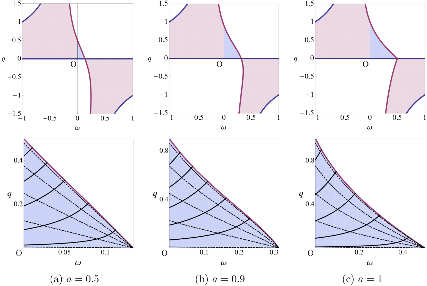
The effective horizon on the induced geometry emerges when the rigidly rotating string regularly passes through a light surface on the spacetime. For a given $\omega$, the effective horizon is uniquely determined, whereas there are several possibilities for the light surfaces; the inner light sphere near the black hole and the outer light cylinder exist, or the single connected light surface does. Therefore, even in the $r^{+}_{\mathrm{eff}}$ branch one should be careful about which light surface the string is passing through. We find critical angular velocities $\omega_{\mathrm{c}}^{\pm}$ ($\omega^{-}_{\mathrm{c}}<0<\omega^{+}_{\mathrm{c}}$), at which the inner and outer light surfaces merge on the equatorial plane, is given by the extrema of $\omega_{\pi/2}(q)$, namely $\omega^{\pm}_{\mathrm{c}}=\omega_{\pi/2}(q^{\pm}_{\mathrm{c}})$ such that $d\omega_{\pi/2}/dq|_{q=q^{\pm}_{\mathrm{c}}}=0$ (see Appendix A.2 for detail). The topology of the light surface changes at $\omega=\omega^{\pm}_{\mathrm{c}}$, while the configurations of the string may continuously deform in terms of the two parameters ($\omega,q$). Hence, the parameter region can be classified into the following three categories based on the light surface passed by the string: (i) the inner light sphere near the black hole when $\omega^{-}_{\mathrm{c}}\leq\omega\leq\omega^{+}_{\mathrm{c}}$ and $q^{+}_{\mathrm{c}}\leq q\leq q^{-}_{\mathrm{c}}$, (ii) the outer light cylinder when $\omega^{-}_{\mathrm{c}}\leq\omega\leq\omega^{+}_{\mathrm{c}}$ and $q\leq q^{+}_{\mathrm{c}},q\geq q^{-}_{\mathrm{c}}$, and (iii) the connected light surface when $\omega\leq\omega^{-}_{\mathrm{c}},\omega\geq\omega^{+}_{\mathrm{c}}$. In addition, the points ($\omega^{\pm}_{\mathrm{c}},q^{\pm}_{\mathrm{c}}$) are the critical points at which the three regions join. A sketch of the parameter region is depicted in Fig. 3. It is worth noting that in the region for $\omega q>0$, which we have been interested in, the effective horizon on the string is the inner light sphere. We can confirm that, when the energy extraction occurs, the string is regularly passing through the inner light sphere and is twining around the black hole.

This result indicates that the energy extraction can occur when the string enters the inside of the ergoregion, and relations between the event horizon and the string configuration such as whether the string would intersect with the event horizon are irrelevant. This is not surprising logically. Outward flux conveying energy to infinity, physically, cannot propagate with exceeding the speed of light. Such energy flux must depend only on its causal past. By the definition of the event horizon, the causal past of energy flux which can reach to infinity does not include the event horizon. Hence, the event horizon is irrelevant to occurrence of the energy extraction by outward energy flux.

For general string configurations with $\omega\neq 0$, we do not have analytic solutions of the equations of motion. To study analytically some global properties of rigidly rotating string configurations, we perform perturbation analysis of the equations of motion by supposing that the rotation of the Kerr black hole is slow, namely $a\ll M$. This perturbation analysis can be regarded as extensions of the work [17] to rigidly rotating string configurations with $\omega\neq 0$ in the slow-rotation regime. We use the same gauge with the one adopted in Ref. [17] for usefulness of comparison with it. Thus the string configuration is given by the embedding $t=\tau+\eta(r)$, $\phi=\omega t+\varphi(r)$, and $\theta=\theta(r)$.⁵⁵ 5 Note that $\eta(r)$ means a gauge choice for a time coordinate $\tau$ on the world sheet, and one can choose $\eta(r)$ so that the induced metric becomes diagonal in these world sheet coordinates, for example. However, the following equations of motion by using only quantities associated with the spacetime coordinates are independent of the gauge choice on the world sheet. The resultant equations of motion are

where

Note that $\Delta$, $\Sigma$, and $F$ have been defined in the previous section. We can reduce Eqs. (20)–(22) to the above equations of motion with a transformation of variables such as $d\theta/dr=\theta^{\prime}/r^{\prime}$, $d\varphi/dr=\varphi^{\prime}/r^{\prime}$, and so on. The solutions of Eqs. (33) and (34) for $\omega=0$ which are regularly crossing the ergosphere were obtained analytically in Ref. [16]. They are explicitly written as

where $\theta_{0}$ is the integration constant related to $q$ as $q=\pm a\sin^{2}\theta_{0}$ and a constant term within $\varphi_{\pm}(r)$ has been discarded thanks to the axisymmetry.

Here we consider string configurations with $\omega\neq 0$ in the slow-rotation regime. We can define two regions in the Kerr spacetime as

Note that the slow-rotation regime $a\ll M$ allows us to take an overlap region between the far and near regions as $M\ll r-r_{\mathrm{h}}\ll M^{2}/a$. Furthermore we assume the following scalings for $\omega$ and $q$:

which mean that the strings, also, are slowly rotating. In this setting, we can neglect the black hole and regard the spacetime as a flat spacetime in the far region at the leading order. At the near region, we can solve Eqs. (33) and (34) by perturbation analysis in the $a/M$ expansions. The outer light cylinder is not located in the near region and the inner light sphere is not in the far region, so that we should obtain regular solutions in each region and match the near-region solutions with the far-region solutions in order to have globally regular solutions.

References

- [1] R. Penrose, “Gravitational collapse: The role of general relativity,” Riv. Nuovo Cim. 1, 252 (1969) [Gen. Rel. Grav. 34, 1141 (2002)].
- [2] R. Penrose and R. M. Floyd, “Extraction of rotational energy from a black hole,” Nature 229, 177 (1971).
- [3] Ya. B. Zel’dovich, “Generation of waves by a rotating body,” Zh. Eksp. Teor. Fiz. 14, 270 (1971) [JETP Lett. 14, 180 (1971)]; “Amplification of cylindrical electromagnetic waves reflected from a rotating body,” Zh. Eksp. Teor. Fiz 62, 2076 (1972) [Sov. Phys. JETP 35, 1085 (1972)].
- [4] J. M. Bardeen, W. H. Press, and S. A. Teukolsky, “Rotating black holes: Locally nonrotating frames, energy extraction, and scalar synchrotron radiation,” Astrophys. J. 178, 347 (1972).
- [5] A. A. Starobinsky, “Amplification of waves during reflection from a rotating “black hole”,” Zh. Eksp. Teor. Fiz 64, 48 (1973) [Sov. Phys. JETP 37, 28 (1973)].
- [6] A. A. Starobinsky and S. M. Churilov, “Amplification of electromagnetic and gravitational waves scattered by a rotating “black hole”, ” Zh. Eksp. Teor. Fiz 65, 3 (1973) [Sov. Phys. JETP 38, 1 (1974)].
- [7] S. A. Teukolsky and W. H. Press, “Perturbations of a rotating black hole. III. Interaction of the hole with gravitational and electromagnetic radiation,” Astrophys. J. 193, 443 (1974).
- [8] R. D. Blandford and R. L. Znajek, “Electromagnetic extractions of energy from Kerr black holes,” Mon. Not. Roy. Astron. Soc. 179, 433 (1977).
- [9] S. M. Wagh, S. V. Dhurandhar and N. Dadhich, “Revival of penrose process for astrophysical applications,” Astrophys. J. 290, no. 12 (1985) [Atrophys. J. 301, 1018 (1986)].
- [10] R. Brito, V. Cardoso and P. Pani, “Superradiance : Energy Extraction, Black-Hole Bombs and Implications for Astrophysics and Particle Physics,” Lect. Notes Phys. 906, pp.1 (2015) [arXiv:1501.06570 [gr-qc]].
- [11] S. S. Gubser, “Drag force in AdS/CFT,” Phys. Rev. D 74, 126005 (2006) [hep-th/0605182].
- [12] V. P. Frolov, “Merger transitions in brane–black-hole systems: Criticality, scaling, and self-similarity,” Phys. Rev. D 74, 044006 (2006) [gr-qc/0604114].
- [13] D. Mateos, R. C. Myers, and R. M. Thomson, “Holographic phase transitions with fundamental matter,” Phys. Rev. Lett. 97, 091601 (2006) [hep-th/0605046].
- [14] V. S. Semenov, “String mechanism for energy extraction from a Kerr black hole,” Phys. Scripta 62, 123 (2000).
- [15] V. S. Semenov, S. A. Dyadechkin, I. B. Ivanov, and H. K. Biernat, “Energy confinement for a relativistic magnetic flux tube in the ergosphere of a Kerr black hole,” Phys. Scripta 65, 13 (2002) [astro-ph/0110168].
- [16] V. P. Frolov, S. Hendy, and A. L. Larsen, “How to create a 2-D black hole,” Phys. Rev. D 54, 5093 (1996) [hep-th/9510231].
- [17] V. P. Frolov, S. Hendy, and J. P. De Villiers, “Rigidly rotating strings in stationary axisymmetric spacetimes,” Class. Quant. Grav. 14, 1099 (1997) [hep-th/9612199].
- [18] K. Ogawa, H. Ishihara, H. Kozaki, H. Nakano, and S. Saito, “Stationary rotating strings as relativistic particle mechanics,” Phys. Rev. D 78, 023525 (2008) [arXiv:0803.4072 [gr-qc]].
- [19] A. Kuiroukidis and D. B. Papadopoulos, “Strings in Kerr-Newmann black holes,” Gen. Rel. Grav. 32, 593 (2000) [gr-qc/9909057].
- [20] P. A. R. Ade et al. (Planck Collaboration), “Planck 2013 results. XXV. Searches for cosmic strings and other topological defects,” Astron. Astrophys. 571, A25 (2014) [arXiv:1303.5085 [astro-ph.CO]].