Axion crystals

The electronic band structure that originates from the periodicity of crystals is essential in determining the electronic properties of materials. Yet the notion of the band structure is not limited to electrons, but can also be extended to photons: a regular array of materials with different dielectric constants (or different refractive indices) leads to the band structure of photons. This is the photonic crystal [1], which is expected to be applied to various optoelectronic devices.

Meanwhile, recent development of topological insulators (see, e.g., refs. [2, 3] for reviews) reveals that, most generically, the low-energy effective theories for all the gapped insulators are classified by not only permittivity $\epsilon$ and permeability $\mu$, but also one more parameter—the theta angle $\theta$. Here $\theta\equiv 0$ and $\theta\equiv\pi$ (modulo $2\pi$), corresponding to normal insulators and topological insulators, are only possible in time-reversal systems [4].

In this paper, we consider a new type of crystals with periodic $\theta$ (modulo $2\pi$) in space, which we call the axion crystals. As the simplest yet nontrivial demonstration that allows for analytic treatment, we study the band structure of photons in one-dimensional axion crystals with the staircase profile of $\theta$ (see figure 1 below). As we will see, this configuration corresponds to the “Kronig-Penney-type potential” for $\bm{\nabla}\theta$.

We find that axion crystals have a number of new features that the usual photonic crystals do not possess. In particular, one of the helicity states acquires a mass gap, even without superconductivity, while the other has the nonrelativistic gapless dispersion relation at small momentum. The presence of such gapped photon and nonrelativistic gapless photon depending on the helicity states in the axion electrodynamics has been recently pointed out in ref. [5] for homogeneous $\bm{\nabla}\theta$ .

This paper is organized as follows. In section 2, we review the generic low-energy effective theory for gapped insulators. We also derive the master equation of the photon for a given configuration of $\theta$. In section 3, we study the properties of the band structure of one-dimensional axion crystals. Section 4 is devoted to discussions. Throughout the paper, we use the units $\hbar=c=e=1$.

We first briefly review the generic low-energy effective theory of insulators. Because the electron has a mass gap in insulators by definition, the only relevant low-energy degrees of freedom are photons described by the gauge field $A^{\mu}$. The effective theory for a given insulator that respects the gauge symmetry and the rotational symmetry in space can be written down up to the second order in derivatives as [6]

Here $\epsilon$, $\mu$, and $\theta$ are some constants that depend on the microscopic details of the system, and $j^{\mu}=(\rho,\bm{j})$ is the electric current density. The quantities $\epsilon$ and $\mu$ are called the permittivity and permeability, respectively, which characterize the violation of the Lorentz invariance in medium, and $\theta$ is called the axion term.

Under the time reversal symmetry (which will be abbreviated as $\cal{T}$ symmetry), the electromagnetic fields are transformed as $\bm{E}\rightarrow\bm{E}$ and $\bm{B}\rightarrow-\bm{B}$. Hence, $\cal{T}$ symmetry is broken for generic $\theta$. Meanwhile, the path integral quantization of the theory (1) shows that all the physical quantities are invariant under the transformation $\theta\rightarrow\theta+2\pi$ (see ref. [7] and references therein). Thanks to this periodicity, $\theta=-\pi$ and $\theta=\pi$ are equivalent; the system respects $\cal{T}$ symmetry when

The insulators with $\theta\equiv 0$ (mod $2\pi$) are normal (or topologically trivial) insulators and those with $\theta\equiv\pi$ (mod $2\pi$) are topological insulators [4]. The modified electrodynamics with the spacetime dependent $\theta=\theta(t,\bm{x})$ is known as the axion electrodynamics [6].

In the following, we shall consider nondispersive media described by the axion electrodynamics (1) with the space-dependent $\theta$ term, $\theta=\theta(\bm{x})$, and constant (space-independent) $\epsilon$ and $\mu$ to demonstrate new features for photons induced by the $\theta$ term alone. We will later consider some specific form of $\theta(\bm{x})$ below (see figure 1), but for a moment we will keep our argument general without restricting the particular form of $\theta$. More generally, one can consider the space-dependent $\epsilon$ and/or $\mu$, as usual photonic crystals, at the same time. One can also consider dispersive media where the electric polarization and magnetization are given by the linear convolutions of the response functions multiplied by the electric and magnetic fields. Such extensions should be straightforward and are left for future work.

The modified Maxwell’s equations in the presence of $\theta(\bm{x})$ that follow from the Lagrangian (1) are given by [6]

The additional contributions to the usual Maxwell’s equations are the anomalous charge in the second term on the right-hand side of eq. (3) and the anomalous Hall effect in the third term on the right-hand side of eq. (4).

Let us consider the propagation of an electromagnetic wave (or a photon) in this type of medium without the source of photons, i.e., $\rho=0$ and $\bm{j}={\bm{0}}$. From eqs. (4) and (6), we get the closed equation for ${\bm{E}}$,

where $v=1/\sqrt{\epsilon\mu}$ is the velocity of the photon in medium.

We assume that $\theta({\bm{x}})$ has the $z$ dependence and consider the photon propagating in the $z$ direction. Then we find the following coupled equations for $E_{x}$ and $E_{y}$:

Since $E_{y}=\pm iE_{x}$ for the positive and negative helicity states of the photon ($h=\pm 1$), these equations become [5]

The temporal translational symmetry allows us to take the Fourier transform with respect to time as

where $\omega$ is the frequency. This is the master equation that determines the behavior of $E_{x}(z)$ (and similarly that of $E_{y}(z)$) for a given configuration of $\partial_{z}\theta(z)$.

We now study the band structure (or dispersion relation) of photons in the axion electrodynamics with periodic $\partial_{z}\theta(z)$ in space. Formally, this is analogous to the calculation of the band structure of electrons by solving the Schrödinger equation in a periodic potential. As the simplest yet nontrivial example which allows for analytical treatment, we here consider the one-dimensional “Kronig-Penney-type potential” for $\partial_{z}\theta(z)$ as depicted in figure 2. Later we will take the limit $b\to 0$ and $c\to\infty$ such that $bc=\pi$. In this case, the “potential” $\partial_{z}\theta(z)$ is expressed as

This corresponds to the staircase configuration of $\theta(z)$ shown in figure 1, which can be regarded as a regular array of trivial insulators with $\theta=2n\pi$ ($n\in\mathbb{Z}$) and topological insulators with $\theta=(2n+1)\pi$ (with the same $\epsilon$ and $\mu$) with lattice constant $a$ in one direction.¹¹ 1 Strictly speaking, without any ${\cal T}$ symmetry breaking, there would be gapless Dirac fermions at the interfaces between trivial and topological insulators, which would invalidate the description of the pure axion electrodynamics above. Here our description of the pure axion electrodynamics should be understood as being valid below the gap of Dirac fermions in the presence of a ${\cal T}$ symmetry breaking perturbation at the interfaces [4]. See also ref. [8] for a similar setup in the context different from the band structure. Note that this configuration of $\theta$ is periodic modulo $2\pi$. We call this type of systems the axion crystals.

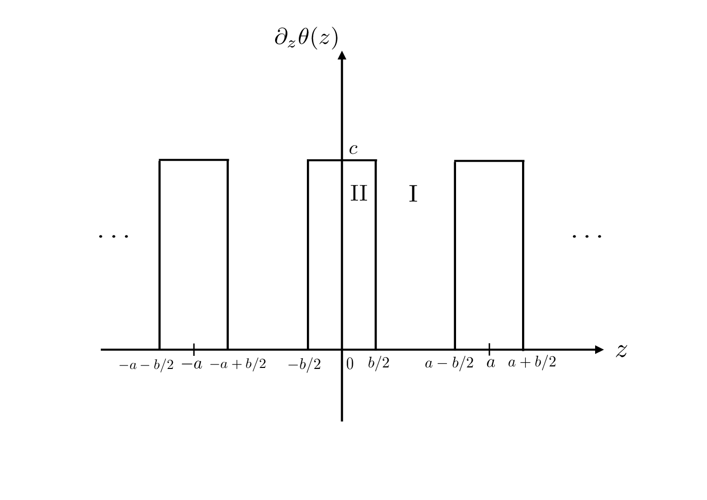
Let us first consider the photon with the helicity state $h=+1$. In the region I ($b/2<z<a-b/2$) where $\partial_{z}\theta(z)=0$, eq. (11) becomes

The generic solution is given by

with some constants $A$ and $B$.

In the region II ($-b/2<z<b/2$) where $\partial_{z}\theta(z)=c$, eq. (11) is

The solution is given by

with some constants $C$ and $D$.

We now impose the boundary conditions at $z=b/2$. Integrating eq. (11) over the interval $[b/2-\delta,b/2+\delta]$ and taking the limit $\delta\rightarrow 0$, it follows that $\partial_{z}E_{x}(z)$ together with $E_{x}(z)$ must be continuous at $z=b/2$. We thus obtain

In addition, as $\partial_{z}\theta(z)$ in eq. (11) is periodic with the period $a$, Bloch’s theorem states that $E_{x}(z)$ satisfies $E_{x}(z+a)=e^{ika}E_{x}(z)$, and consequently, $\partial_{z}E_{x}(z+a)=e^{ika}\partial_{z}E_{x}(z)$. These conditions at $z=-b/2$ lead to

Equations (17)–(20) can be summarized in the matrix equation, ${\cal M}_{ij}x^{j}=0$, where

It has a nontrivial solution as long as the condition, $\det{\cal M}=0$, is satisfied.

This condition is simplified in the limit $b\to 0$ and $c\to\infty$ with keeping $bc=\pi$, corresponding to the profile of $\theta(z)$ in figure 1. After a straightforward calculation, we get

for $h=+1$. Similarly, we have

for $h=-1$. The second terms on the right-hand sides of eqs. (31) and (32) originate from the $\theta$ term, which distinguishes the two helicity states of photons.

Without the $\theta$ term, two equations above become degenerate, $\cos(ka)=\cos(Ka)$, reducing to the usual dispersion relation of the photon in medium,

However, the presence of the periodic $\theta$ term gives rise to a nontrivial band structure of photons, analogously to that of electrons in a periodic potential, and further to a band structure splitting between the two helicity states of photons as a consequence of the parity-violating nature of the $\theta$ term, unlike usual photonic crystals.

From eqs. (31) and (32), we plot the band structure of photons with each helicity $h=\pm 1$ in figure 3. One observes that, for each helicity, there is a range of frequency—the photonic band gaps at $ka/\pi=n$ ($n=0,1,2,\cdots$)—where no photon eigenmode exists. This feature is similar to that in usual photonic crystals. To understand the origin of these band gaps, we plot the right-hand sides of the eqs. (31) and (32) as a function of $Ka$ in figure 4. Since the left-hand sides of both equations is bounded as $-1\leq\cos(ka)\leq+1$, the solutions do not exist when the right-hand sides are outside of this region for some $Ka$. The absence of the solutions suggests the presence of the photonic band gaps for such $Ka$.

Using eqs. (31) and (32), one can show that the magnitudes of the photonic band gaps for the helicity $h=\pm 1$ at $ka/\pi=n$, which we define as $\Delta_{n}^{\pm}>0$, are all equivalent, except for $h=+1$ and $n=0$ (for which the photonic band gap is absent). Indeed, such $\Delta_{n}^{\pm}$ satisfies the same equation,

independently of $n$ and the helicity $h=\pm 1$ (except for $h=+1$ and $n=0$), and one can set $\Delta_{n}^{\pm}=\Delta$. Equation (34) can be easily solved in terms of $\Delta$ as

Note that $0\leq 2p/(p^{2}+1)\leq 1$ for any $p>0$.

In summary, we obtain the photonic band gaps for each helicity $h=\pm 1$ as follows:

where $\Delta$ is given by eq. (35).

It is interesting to note that there exists a special value $p=1$, or

where the photonic band gaps are always open for either only one of the two helicity states of photons. In this case, the photonic band gaps are

Let us closely look at the properties of the band structure of photons at small $k$ in axion crystals.

First, as we have seen above, one of the helicity states ($h=-1$) is gapped at $k=0$. Remarkably, the photon here acquires a mass gap even in the absence of superconductivity or the so-called Englert-Brout-Higgs mechanism. While mass gap generation for gauge fields due to the Chern-Simons term in $2+1$ spacetime dimensions has been known [9], our result provides a new mechanism of helicity-dependent mass gap generation due to the axion term in $3+1$ dimensions.

Second, the other gapless helicity state ($h=+1$) does not have a relativistic dispersion relation. By performing the expansion in small $k$ and $\omega$ in eq. (31), we obtain

Just like the usual relativistic photon with the dispersion relation $\omega=k$ can be regarded as the (type-I) Nambu-Goldstone mode [11, 12], this “nonrelativistic photon” may be understood as the so-called type-II Nambu-Goldstone mode [5, 13].

The appearances of the gapped photon and nonrelativistic gapless photon depending on the helicity states are the novel features that are absent in usual photonic crystals.

In this paper, we have studied the band structure of photons in axion crystals. Although we have focused here on a one-dimensional axion crystal as a demonstration, one can consider axion crystals in two and three dimensions. Our simple model could also be made more realistic by relaxing the condition of the homogeneous permittivity and/or permeability.

The axion crystal should be realized by stacking trivial insulators with $\theta=2n\pi$ ($n\in\mathbb{Z}$) and topological insulators with $\theta=(2n+1)\pi$ alternately. The helicity-dependent band structure of the axion crystal suggests that electromagnetic waves with one of the circularly polarizations and with frequencies within the photonic band gaps incident in the direction of the modulation of $\theta$ are perfectly reflected. Hence, the axion crystal behaves as a polarizer that transmits electromagnetic waves with only one polarization within these frequency regions. One could, in principle, tune the region and the magnitude of the photonic band gaps by changing the lattice constant $a$ [see eq. (35)]. This property may be useful for applications in possible new optoelectronic devices.

The axion crystals may be relevant in high-energy physics as well. It has been recently found that the ground state of Quantum Chromo Dynamics (QCD) at finite baryon chemical potential in a strong magnetic field becomes the chiral soliton lattice of neutral pions, characterized by the periodic $\langle\bm{\nabla}\pi^{0}\rangle$ in space [14]. Then the Wess-Zumino-Witten term $\pi^{0}\bm{E}\cdot\bm{B}$ leads to the axion electrodynamics in QCD matter [5] (see also ref. [15]), where the periodic $\langle\bm{\nabla}\pi^{0}\rangle$ exactly plays the role of the periodic $\bm{\nabla}\theta$ considered in this paper. In this way, the chiral soliton lattice in QCD provides an explicit realization of the axion crystal. Such a state is potentially realized in dense matter inside neutron stars with a strong magnetic field.

The author N. Y. thanks T. Brauner and Y. Hidaka for useful conversations. This work was supported by JSPS KAKENHI Grant No. 16K17703 and MEXT-Supported Program for the Strategic Research Foundation at Private Universities, “Topological Science” (Grant No. S1511006).

References

- (1) J. D. Joannopoulos, S. G. Johnson, J. N. Winn and R. D. Meade, Photonic Crystals: Molding the Flow of Light (Princeton University Press, Princeton, 2008).
- (2) M. Z. Hasan and C. L. Kane, Rev. Mod. Phys. 82, 3045 (2010) [arXiv:1002.3895 [cond-mat.mes-hall]].
- (3) X. L. Qi and S. C. Zhang, Rev. Mod. Phys. 83, 1057 (2011).
- (4) X. L. Qi, T. L. Hughes and S. C. Zhang, Phys. Rev. B 78, 195424 (2008) [arXiv:0802.3537 [cond-mat.mes-hall]].
- (5) N. Yamamoto, Phys. Rev. D 93, 085036 (2016) [arXiv:1512.05668 [hep-th]].
- (6) F. Wilczek, Phys. Rev. Lett. 58, 1799 (1987).
- (7) M. M. Vazifeh and M. Franz, Phys. Rev. B 82, 233103 (2010) [arXiv:1006.3355 [cond-mat.mes-hall]].
- (8) R. Zeng, L. Chen, W. Nie, M. Bi, Y. Yang and S. Zhu, Phys. Lett. A 380, 2861 (2016).
- (9) S. Deser, R. Jackiw and S. Templeton, Phys. Rev. Lett. 48, 975 (1982);
- (10) S. Deser, R. Jackiw and S. Templeton, Annals Phys. 140, 372 (1982).
- (11) R. Ferrari and L. E. Picasso, Nucl. Phys. B 31, 316 (1971).
- (12) R. A. Brandt and W. C. Ng, Phys. Rev. D 10, 4198 (1974).
- (13) Y. Hidaka, private communication.
- (14) T. Brauner and N. Yamamoto, JHEP 1704, 132 (2017) [arXiv:1609.05213 [hep-ph]].
- (15) E. J. Ferrer and V. de la Incera, arXiv:1512.03972 [nucl-th].