跳到论文正文
W Papers独立论文阅读器 arXiv:1610.07683 论文正文 计算阅读时间 · 0%
引用这篇论文根据当前论文元数据生成,正式投稿前建议核对。


License: arXiv.org perpetual non-exclusive license
arXiv:1610.07683v1 [stat.ME] 24 Oct 2016
11footnotetext: Research supported in part by NSF FRG Grant DMS-1265202, and NIH Grant 1-U54AI117924-01.22footnotetext: Address for Correspondence: Department of Statistics, University of Wisconsin-Madison, 1300 University Avenue, Madison, WI 53706.

Combined Hypothesis Testing on Graphs with Applications to Gene Set Enrichment Analysis∗

Shulei Wang    Ming YuanMorgridge Institute for Research and University of Wisconsin-Madison
(August 24, 2026)
Abstract

Motivated by gene set enrichment analysis, we investigate the problem of combined hypothesis testing on a graph. We introduce a general framework to effectively use the structural information of the underlying graph when testing multivariate means. A new testing procedure is proposed within this framework. We show that the test is optimal in that it can consistently detect departure from the collective null at a rate that no other test could improve, for almost all graphs. We also provide general performance bounds for the proposed test under any specific graph, and illustrate their utility through several common types of graphs. Numerical experiments are presented to further demonstrate the merits of our approach.

1 Introduction

Combined hypothesis testing arises naturally in many modern statistical applications. See Chapter 9 of Efron (2013) for further discussions. The most notable example is the so-called gene set enrichment analysis. See, e.g., Mootha et al. (2003), Subramanian et al. (2005), Tian et al. (2005), Efron and Tibshirani (2007), Goeman and Bühlmann (2007), Jiang and Gentleman (2007), Newton et al. (2007), and Ackermann and Strimmer (2009) among many others. It is motivated by the observation that many complex diseases are manifested through modest regulation in a set of related genes rather than a strong effect on a single gene. While statistical testing of the regulatory effect on a particular gene may be inconclusive, the collective effect on a set of genes can oftentimes be clearly identified through combined hypothesis testing. The results produced by gene set enrichment analysis could therefore be more reliable and biologically meaningful when compared with those based on a single gene. Given its importance in statistical genomics, gene set enrichment analysis has attracted much attention in recent years and numerous approaches have been proposed. See Maciejewski (2013) and Newton and Wang (2015) for a couple of recent surveys on existing techniques.

Most statistical methods for gene set enrichment analysis proceed in two steps. One first computes for each gene a local statistic, i.e., for testing if a gene is differentially expressed between multiple biological conditions. For concreteness, denote by VV the index set of a particular collection of related genes, and xvx_{v} the zz-score associated with the vvth gene so that

xv=μv+ϵv,v∈V,x_{v}=\mu_{v}+\epsilon_{v},\qquad v\in V,

where ϵv∼N⁡(0,1)\epsilon_{v}\sim N(0,1). In the second step, we consider testing a combined null hypothesis that there is no effect on the gene set, that is

H0:μv=0,∀v∈V,H_{0}:\mu_{v}=0,\qquad\forall v\in V, (1)

against an overall effect:

Ha:𝝁=(μv)v∈V≠𝟎.H_{a}:\mbox{\boldmath$\mu$}=(\mu_{v})_{v\in V}\neq{\bf 0}. (2)

See, e.g., Efron (2013).

A rich source of information often neglected in these analyses is the fact that a gene set is typically taken from a certain biological pathway, be it a metabolic pathway or a signaling pathway, describing a series of biochemical and molecular steps towards a specific biological function. Many of the known pathways are now readily accessible through several well-curated databases such as Gene Ontology (Ashburner et al., 2000), KEGG (Kanehisa and Goto, 2000), or Pathguide (Bader et al., 2006). A pathway can be conveniently represented by a graph G=(V,E)G=(V,E) where each node v∈Vv\in V corresponds to a gene, and an edge (v1,v2)∈E(v_{1},v_{2})\in E between a pair of nodes indicates direct interactions between them. It is, however, largely unknown to what extent such pathway information could be utilized in gene set enrichment analysis. The main goal of this article is to address this issue, and develop a principled and effective way to take advantage of such structural information for gene set enrichment analysis in particular and combined hypothesis testing in general.

More specifically, we introduce a hierarchy among all possible effects based on their level of smoothness with respect to the underlying pathway, and argue that the difficulty in testing against a particular effect 𝝁(≠0)\mbox{\boldmath$\mu$}(\neq 0) depends critically on its smoothness in that “smoother” effects are “easier” to detect. We note, that unlike functions defined over a continuous domain, smoothness is an innocuous concept here because any 𝝁∈ℝ|V|\mbox{\boldmath$\mu$}\in\mathbb{R}^{|V|} can be associated with a finite smoothness index. This framework allows us to exploit the fact that, in many applications, it is plausible that a putative effect is sufficiently “smooth”. But at the first glance, such an observation may have little practical implication because even if the effect is indeed smooth, one rarely knows how smooth it might be. We show here that despite the absence of such knowledge regarding 𝝁\mu’s smoothness, it is still possible to develop an agnostic test that automatically adapts to it. In particular, we develop an easily implementable adaptive testing procedure whose power increases automatically with the smoothness of the unknown 𝝁\mu.

To demonstrate the merits of the proposed paradigm and test, we study its asymptotic properties from two different and complementary aspects: an average-case analysis based on Erdös-Rényi model; and a general analysis that applies to any specific type of graphs. The former analysis shows that among all graphs of nn nodes, with the exception of a vanishing proportion of graphs under Erdös-Rényi model, the proposed test is minimax optimal for any level of smoothness in that one cannot do better over all effects at the same level of smoothness even if we know in advance how smooth they are. In addition, we derive a generally applicable performance bound for our test and illustrate through several fundamental types of graph its utility and optimality.

Although we focus our discussion primarily in the context of gene set enrichment analysis, it is worth noting that the methodology and theory we developed here may also be useful in many other applications. For example, one may be interested in performing combined hypothesis testing over locations within a particular region of the brain, as a means to identifying areas that can be associated with certain activities. See, e.g., Chung et al. (2016). In these situations, it is plausible that an overall effect is smooth with respect to the brain surface manifold. This can be translated into smoothness with respect to nearest neighbor graphs underlying these locations. The techniques developed here can then be employed in these applications.

The rest of the paper is organized as follows. We first introduce the general framework of our treatment and the proposed test in Section 2. In Section 3 we investigate the properties of the proposed tests under the Erdös-Rényi model to gain insights into their operating characteristics as well as the effect of smoothness on the detectability of a particular effect. Section 4 provides general performance bounds for our tests, and their applications to several common types of graphs. Numerical experiments are presented in Section 5 to further demonstrate the merits of the proposed methodology. All proofs are relegated to Section 6.

2 Methodology

A natural approach to testing H0H_{0} against HaH_{a} given by Equations (1) and (2) respectively is a χ2\chi^{2}-test based on the statistic

‖𝐗‖2:=∑vXv2\|\mathbf{X}\|^{2}:=\sum_{v}X_{v}^{2}

where 𝐗=(Xv)v∈V\mathbf{X}=(X_{v})_{v\in V}. It is clear that under H0H_{0}, ‖𝐗‖2\|\mathbf{X}\|^{2} follows a χ|V|2\chi^{2}_{|V|} distribution, so that a α\alpha-level test rejects H0H_{0} if and only if ‖𝐗‖2\|\mathbf{X}\|^{2} exceeds the (1−α)(1-\alpha) quantile, denoted by χ|V|,α2\chi^{2}_{|V|,\alpha}, of χ|V|2\chi^{2}_{|V|} distribution. Here |⋅||\cdot| denotes the cardinality of a set. On the other hand, under the alternative hypothesis, 𝐗∼N⁡(𝝁,I)\mathbf{X}\sim N(\mbox{\boldmath$\mu$},I) so that ‖𝐗‖2\|\mathbf{X}\|^{2} follows a non-central χ|V|2​(‖𝝁‖2)\chi^{2}_{|V|}(\|\mbox{\boldmath$\mu$}\|^{2}) distribution. Denote by φχ2,α\varphi_{\chi^{2},\alpha} the α\alpha-level χ2\chi^{2}-test. Hereafter, we shall omit the subscript α\alpha and write φχ2\varphi_{\chi^{2}} for brevity, when no confusion occurs. It is clear that the Type II error of φχ2\varphi_{\chi^{2}} is given by

β(φχ2;𝝁):=ℙ𝐗∼N⁡(𝝁,I){∥𝐗∥2>χ|V|,α2}.\beta(\varphi_{\chi^{2}};\mbox{\boldmath$\mu$}):=\mathbb{P}_{\mathbf{X}\sim N(\mbox{\boldmath$\mu$},I)}\left\{\|\mathbf{X}\|^{2}>\chi^{2}_{|V|,\alpha}\right\}.

It is not hard to see that β⁡(φχ2,𝝁)\beta(\varphi_{\chi^{2}};\mbox{\boldmath$\mu$}) goes to zero as soon as ‖𝝁‖2≫|V|1/2\|\mbox{\boldmath$\mu$}\|^{2}\gg|V|^{1/2}, where aV≫bVa_{V}\gg b_{V} means aV/bV→∞a_{V}/b_{V}\to\infty as |V|→∞|V|\to\infty. In other words, φχ2\varphi_{\chi^{2}} can consistently detect all effects 𝝁\mu such that

‖𝝁‖2≫|V|1/2.\|\mbox{\boldmath$\mu$}\|^{2}\gg|V|^{1/2}. (3)

Furthermore, it is well known that the χ2\chi^{2}-test is minimax optimal in testing H0H_{0} against HaH_{a} in that the detection boundary given by (3) cannot be improved. More precisely, there exists a constant c>0c>0 such that for any α\alpha-level (0<α<10<\alpha<1) test Ψ\Psi based on 𝐗\mathbf{X},

lim inf|V|→∞sup𝝁:‖𝝁‖2≥c​|V|1/2β(Ψ,𝝁)>0.\liminf_{|V|\to\infty}\sup_{\mbox{\boldmath$\mu$}:\|\mbox{\boldmath$\mu$}\|^{2}\geq c|V|^{1/2}}\beta(\Psi,\mbox{\boldmath$\mu$})>0.

See, e.g., Ingster and Suslina (2003) for further discussions.

Despite the minimax optimality of χ2\chi^{2}-test, there is also ample empirical evidence that other tests, such as zz-test, may work better in some situations. This is because the optimality of χ2\chi^{2}-test is in the minimax sense, and therefore based on the worst-case performance. Although the minimax optimality suggests that no test could do better than φχ2\varphi_{\chi^{2}} over all effects 𝝁∈ℝ|V|∖{𝟎}\mbox{\boldmath$\mu$}\in\mathbb{R}^{|V|}\setminus\{{\bf 0}\}, it does not necessarily preclude improvements over subsets of ℝ|V|\mathbb{R}^{|V|}. For example, if 𝝁∝𝟏\mbox{\boldmath$\mu$}\propto\mathbf{1}, where 𝟏{\bf 1} is the vector of ones, then zz-test is a more powerful test than χ2\chi^{2}-test and it can detect any 𝝁\mu of this form as long as ‖𝝁‖→∞\|\mbox{\boldmath$\mu$}\|\to\infty. In fact, zz-test is the most powerful test in this situation by Neyman-Pearson Lemma. Unfortunately, such an improvement over χ2\chi^{2}-test comes at a hefty price – zz-test is powerless in testing against any effect 𝝁\mu such that 𝝁⊤​𝟏=0\mbox{\boldmath$\mu$}^{\top}\mathbf{1}=0 in that

β⁡(φz,𝝁)=1−α\beta(\varphi_{z};\mbox{\boldmath$\mu$})=1-\alpha

where φz\varphi_{z} denotes the α\alpha-level zz-test.

This naturally brings about the question of whether or not the strengths of zz-test and χ2\chi^{2}-test could be combined. We show that this indeed is possible, and develop a test that is just as powerful as the χ2\chi^{2}-test in the absence of any information regarding a putative effect, but could be as powerful as the zz-test when the effect is indeed a constant. More generally, the test could be substantially more powerful than the χ2\chi^{2}-test depending on the smoothness of the unknown effect with respect to the graph G=(V,E)G=(V,E). This is of particular interest here because in many applications of gene set enrichment analysis, it is plausible that the effect 𝝁\mu is of certain level of smoothness with respect to the graph GG. Our framework here is largely inspired by the pioneering work of Ingster (1993) on nonparametric testing. See also Ingster and Suslina (2003).

Recall that the Laplacian matrix of GG is given by

L⁡(G)=D⁡(G)−A⁡(G)L(G)=D(G)-A(G)

where D⁡(G)D(G) and A⁡(G)A(G) are its degree matrix and adjacency matrix respectively. To fix ideas, we shall focus on unweighted and undirected graphs, although our treatment can also be applied to more general, e.g., weighted or directed, graphs. For an unweighted and undirected graph GG, the adjacency matrix A⁡(G)A(G) is a symmetric matrix whose (v,v′)(v,v^{\prime}) entry is one if (v,v′)∈E(v,v^{\prime})\in E and zero otherwise, and the degree matrix D⁡(G)D(G) is a diagonal matrix whose vvth diagonal entry is the degree of node vv. It is clear that

𝝁⊤​L​(G)​𝝁=∑(v1,v2)∈E(μv1−μv2)2,\mbox{\boldmath$\mu$}^{\top}L(G)\mbox{\boldmath$\mu$}=\sum_{(v_{1},v_{2})\in E}(\mu_{v_{1}}-\mu_{v_{2}})^{2}, (4)

so that it measures the smoothness of 𝝁\mu with respect to GG. The smoothness of 𝝁\mu with respect to graph GG allows us to create a hierarchy in ℝ|V|\mathbb{R}^{|V|}. More specifically, for an arbitrary η2≥0\eta^{2}\geq 0, denote by ΘG​(η2)\Theta_{G}(\eta^{2}) the collection of all effects whose smooth index as defined by (4) is at most η2\eta^{2}, that is,

ΘG​(η2)={𝝁∈ℝn:𝝁⊤​L​(G)​𝝁≤η2}.\Theta_{G}(\eta^{2})=\{\mbox{\boldmath$\mu$}\in\mathbb{R}^{n}:\mbox{\boldmath$\mu$}^{\top}L(G)\mbox{\boldmath$\mu$}\leq\eta^{2}\}. (5)

For brevity, we shall omit the subscript GG in what follows when no confusion occurs. Obviously, the smaller η2\eta^{2} is, the smaller Θ⁡(η2)\Theta(\eta^{2}) is, as illustrated in Figure 1. Thus, it is natural to expect it to be easier to detect effects from Θ⁡(η2)\Theta(\eta^{2}) for smaller η2\eta^{2}s. In particular, since χ2\chi^{2}-test is optimal for testing against an arbitrary effect 𝝁∈Θ⁡(+∞)=ℝ|V|\mbox{\boldmath$\mu$}\in\Theta(+\infty)=\mathbb{R}^{|V|}, we might expect to be able to improve it over Θ⁡(η2)\Theta(\eta^{2}) for any finite η2\eta^{2}. It turns out, however, not to be the case.

𝝁=0\mbox{\boldmath$\mu$}=0ΘG​(η12)\Theta_{G}(\eta_{1}^{2})ΘG​(η22)\Theta_{G}(\eta_{2}^{2})ΘG​(+∞)\Theta_{G}(+\infty)⋯<η12<η22<⋯\cdots<\eta_{1}^{2}<\eta_{2}^{2}<\cdots
Figure 1: Smoothness creates an hierarchy among all effects in ℝ|V|\mathbb{R}^{|V|}.
Theorem 1.

Let ηmax2(G)=|V|−1/2trace(L(G))\eta_{\max}^{2}(G)=|V|^{-1/2}\mathrm{trace}(L(G)) where L⁡(G)L(G) is the Laplacian of a graph G=(V,E)G=(V,E). Then for any η2=Ω⁡(ηmax2​(G))\eta^{2}=\Omega(\eta_{\max}^{2}(G)) there exists a constant c>0c>0 such that for any α\alpha-level (0<α<10<\alpha<1) test Ψ\Psi,

lim inf|V|→∞sup𝝁∈ΘG​(η2):‖𝝁‖2≥c​|V|1/2β(Ψ;𝝁)>0.\liminf_{|V|\to\infty}\sup_{\mbox{\boldmath$\mu$}\in\Theta_{G}(\eta^{2}):\|\mbox{\boldmath$\mu$}\|^{2}\geq c|V|^{1/2}}\beta(\Psi;\mbox{\boldmath$\mu$})>0.

Hereafter, we write aV=Ω⁡(bV)a_{V}=\Omega(b_{V}) if bV=O⁡(aV)b_{V}=O(a_{V}). Theorem 1, together with the fact that χ2\chi^{2}-test is consistent for any 𝝁∈ℝ|V|\mbox{\boldmath$\mu$}\in\mathbb{R}^{|V|} such that ‖𝝁‖2≫|V|1/2\|\mbox{\boldmath$\mu$}\|^{2}\gg|V|^{1/2}, suggests that one cannot improve over χ2\chi^{2}-test for sufficiently large, albeit finite, η2\eta^{2}s. However, it indeed is possible to do so for smaller η2\eta^{2}s. The biggest gain, not surprisingly, occurs when η=0\eta=0.

Let KK be the number of connected components in GG, and Gk=(Vk,Ek)G_{k}=(V_{k},E_{k}), k=1,…,Kk=1,\ldots,K, the components so that G=∪kGkG=\cup_{k}G_{k}. In this setting, L⁡(G)L(G) has exactly KK zero eigenvalues corresponding to eigenvectors

𝐯k:=|Vk|−1/2(𝕀(v∈Vk))v∈V,k=1,…,K,\mathbf{v}_{k}:=|V_{k}|^{-1/2}(\mathbb{I}(v\in V_{k}))_{v\in V},\qquad k=1,\ldots,K,

where 𝕀\mathbb{I} is the characteristic function that takes value 1 if the the condition holds and zero otherwise. Thus,

Θ(0)={𝝁=c1𝐯1+⋯+cK𝐯K:c1,…,cK∈ℝ},\Theta(0)=\left\{\mbox{\boldmath$\mu$}=c_{1}\mathbf{v}_{1}+\cdots+c_{K}\mathbf{v}_{K}:c_{1},\ldots,c_{K}\in\mathbb{R}\right\},

is a KK dimensional linear subspace of ℝ|V|\mathbb{R}^{|V|}. To test against the effect 𝝁≠0\mbox{\boldmath$\mu$}\neq 0 then amounts to testing against (c1,…,cK)⊤≠𝟎(c_{1},\ldots,c_{K})^{\top}\neq{\bf 0}. By Neyman-Pearson Lemma, the likelihood ratio test is the most power for such a purpose. More specifically, it is not hard to derive the likelihood ratio test statistic

R:=∑k=1K(𝐗⊤​𝐯k)2=∑k=1K[|Vk|−1​(∑v∈VkXv)2].R:=\sum_{k=1}^{K}\left(\mathbf{X}^{\top}\mathbf{v}_{k}\right)^{2}=\sum_{k=1}^{K}\left[|V_{k}|^{-1}\left(\sum_{v\in V_{k}}X_{v}\right)^{2}\right]. (6)

Under H0H_{0}, it is not hard to see that R∼χK2R\sim\chi^{2}_{K}, so that a α\alpha level test would reject H0H_{0} if and only if R≥χK,α2R\geq\chi^{2}_{K,\alpha}. As before, we denote this test by φR,α\varphi_{R,\alpha}, or φR\varphi_{R} for short. We note that when GG is connected, that is K=1K=1, φR\varphi_{R} is equivalent to the zz-test φz\varphi_{z}. On the other hand, under HaH_{a} with the overall effect 𝝁∈Θ⁡(0)\mbox{\boldmath$\mu$}\in\Theta(0), we get L∼χK2​(‖𝝁‖2)L\sim\chi^{2}_{K}(\|\mbox{\boldmath$\mu$}\|^{2}). Thus, RR is consistent for testing against 𝝁∈Θ⁡(0)\mbox{\boldmath$\mu$}\in\Theta(0) if ‖𝝁‖2≫K1/2\|\mbox{\boldmath$\mu$}\|^{2}\gg K^{1/2}. It turns out this is not only the best we can do for Θ⁡(0)\Theta(0), but also for Θ⁡(η2)\Theta(\eta^{2}) with a sufficiently small η2\eta^{2}, in general.

Theorem 2.

Let G=(V,E)G=(V,E) be the union of KK connected and non-overlapped subgraphs, and ηmin2​(G)\eta_{\min}^{2}(G) be the smallest nonzero eigenvalue of its Laplacian L⁡(G)L(G). Then, for any η2=O⁡(ηmin2)\eta^{2}=O(\eta_{\min}^{2}), φR\varphi_{R} is consistent for testing against any 𝛍∈Θ⁡(η2)\mbox{\boldmath$\mu$}\in\Theta(\eta^{2}) such that ‖𝛍‖2≫K1/2\|\mbox{\boldmath$\mu$}\|^{2}\gg K^{1/2} in that β⁡(φR,𝛍)→0\beta(\varphi_{R};\mbox{\boldmath$\mu$})\to 0.

Recall that Θ⁡(0)⊂Θ⁡(ηmin2)\Theta(0)\subset\Theta(\eta_{\min}^{2}) and there is no consistent test against 𝝁∈Θ⁡(0)\mbox{\boldmath$\mu$}\in\Theta(0) obeying ‖𝝁‖2=O⁡(K1/2)\|\mbox{\boldmath$\mu$}\|^{2}=O(K^{1/2}). Thus Theorem 2 shows the optimality of φR\varphi_{R} for testing against 𝝁∈Θ⁡(ηmin2)\mbox{\boldmath$\mu$}\in\Theta(\eta_{\min}^{2}). Comparing the required strength of 𝝁\mu characterized by Theorems 1 and 2, we can see the tremendous advantage of knowing that an effect 𝝁\mu is sufficiently smooth with respect to GG, e.g., 𝝁⊤​L​(G)​𝝁≤ηmin2\mbox{\boldmath$\mu$}^{\top}L(G)\mbox{\boldmath$\mu$}\leq\eta_{\min}^{2}.

However, it is also clear from the above discussion that different tests may be needed to fully exploit the smoothness of 𝝁\mu. Although it is plausible that an overall effect is smooth with respect to GG, such knowledge is rarely known beforehand. Naturally, one may ask if there is an agnostic approach that does not require such knowledge yet can still automatically exploit the potential smoothness of a putative effect, a task akin to adaption in nonparametric testing (Ingster and Suslina, 2003, see, e.g.,). To this end, we consider a class of test statistics designed to account for different levels of smoothess:

Tλ:=𝐗⊤​(I+λ​L​(G))−1​𝐗−trace⁡[(I+λ​L​(G))−1]{trace⁡[(I+λ​L​(G))−2]}1/2,T_{\lambda}:={\mathbf{X}^{\top}(I+\lambda L(G))^{-1}\mathbf{X}-\mathrm{trace}[(I+\lambda L(G))^{-1}]\over\left\{\mathrm{trace}[(I+\lambda L(G))^{-2}]\right\}^{1/2}}, (7)

where λ≥0\lambda\geq 0 is a regularization parameter. The test statistic TλT_{\lambda} is a normalized version of the quadratic form:

𝐗⊤​(I+λ​L​(G))−1​𝐗,\mathbf{X}^{\top}(I+\lambda L(G))^{-1}\mathbf{X},

which can be viewed as the χ2\chi^{2} statistic regularized by the graph Laplacian L⁡(G)L(G). In particular, when λ=0\lambda=0, T0T_{0} is a normalized version of the χ2\chi^{2} statistic and therefore is the most powerful for detecting effects that are not necessarily smooth with respect to GG. On the other hand, when λ→∞\lambda\to\infty, T∞T_{\infty} is a normalized version of the likelihood ratio statistic defined in (6) which is most powerful for testing against a sufficiently smooth effect 𝝁\mu. In general, it is expected that different tuning parameters are suitable for testing against effects of different levels of smoothness.

Not knowing the exact smoothness of 𝝁\mu, we seek the maximum over the whole class of test statistics, leading to the following test statistic:

Tmax=maxλ≥0⁡Tλ.T_{\max}=\max_{\lambda\geq 0}T_{\lambda}. (8)

In general, the distribution of TmaxT_{\max} under H0H_{0} may not be computed analytically. However, it can be readily evaluated by Monte Carlo simulation, or through permutation test in the context of gene set enrichment analysis. Denote by qαq_{\alpha} the 1−α1-\alpha quantile of the null distribution of TmaxT_{\max}, and we proceed to reject H0H_{0} if and only if Tmax>qαT_{\max}>q_{\alpha}. As usual, we shall hereafter denote this test by φT,α\varphi_{T,\alpha}, or φT\varphi_{T} for short, when no confusion occurs.

3 Average-Case Analysis

To appreciate the merits and understand the operating characteristics of the proposed test statistic TmaxT_{\max}, it is illuminating to begin with the case when GG is a random graph, more specifically, an Erdös-Rényi graph. Under the Erdös-Rényi model E​R​(n,p)ER(n,p), first introduced in 1959 (Erdös and Rényi, 1959), a random graph of nn nodes is constructed by connecting each pair of nodes randomly: each edge is included in the graph with probability pp independently. Assuming that the underlying graph GG follows an Erdös-Rényi model, we can work out an explicit form for the asymptotic distribution of TmaxT_{\max}. Denote by μ¯=𝝁⊤​𝟏/n\bar{\mu}=\mbox{\boldmath$\mu$}^{\top}\mathbf{1}/n the average of the coordinates of 𝝁\mu, and 𝝁c=𝝁−μ¯​𝟏\mbox{\boldmath$\mu$}_{c}=\mbox{\boldmath$\mu$}-\bar{\mu}\mathbf{1} the centered version of 𝝁\mu.

Theorem 3.

Let GnG_{n} be a sequence of Erdös-Rényi graphs with nn nodes and a fixed probability of edge inclusion p∈(0,1)p\in(0,1), and TmaxT_{\max} be defined by (7) and (8). Assume that 𝐗∼N⁡(𝛍,I)\mathbf{X}\sim N(\mbox{\boldmath$\mu$},I) such that

δ12=limn→∞1n−1​‖𝝁c‖2,andδ2=limn→∞n​μ¯.\delta_{1}^{2}=\lim_{n\to\infty}{1\over\sqrt{n-1}}\|\mbox{\boldmath$\mu$}_{c}\|^{2},\qquad{\rm and}\qquad\delta_{2}=\lim_{n\to\infty}\sqrt{n}\bar{\mu}.

Then

Tmax→d{(2​Y12+(Y22−1)2)1/2if​Y1>0,Y22>1max⁡{2​Y1,Y22−1}otherwise,asn→∞,T_{\max}\to_{d}\left\{\begin{array}[]{ll}(2Y_{1}^{2}+(Y_{2}^{2}-1)^{2})^{1/2}&{\rm if\ }Y_{1}>0,Y_{2}^{2}>1\\ \max\left\{\sqrt{2}Y_{1},Y_{2}^{2}-1\right\}&{\rm otherwise}\end{array}\right.,\qquad{\rm as}\quad n\to\infty, (9)

where Y1∼N⁡(δ12,1)Y_{1}\sim N(\delta_{1}^{2},1) and Y2∼N⁡(δ2,1)Y_{2}\sim N(\delta_{2},1) are two independent normal random variables. In particular, if 𝐗∼N⁡(0,I)\mathbf{X}\sim N(0,I), then

Tmax→d{(2​Z12+(Z22−1)2)1/2if​Z1>0,Z22>1max⁡{2​Z1,Z22−1}otherwise,asn→∞,T_{\max}\to_{d}\left\{\begin{array}[]{ll}(2Z_{1}^{2}+(Z_{2}^{2}-1)^{2})^{1/2}&{\rm if\ }Z_{1}>0,Z_{2}^{2}>1\\ \max\left\{\sqrt{2}Z_{1},Z_{2}^{2}-1\right\}&{\rm otherwise}\end{array}\right.,\qquad{\rm as}\quad n\to\infty, (10)

where Z1Z_{1} and Z2Z_{2} are two independent standard normal random variables.

Equation (10) allows us to compute more explicitly the critical value of a test based on TmaxT_{\max} at a prescribed significance level, at least in an asymptotic sense. Together with (9), this allows us to more precisely characterize the (asymptotic) power of φT\varphi_{T}. In particular, the power of the 5%5\%-level test, as a function of δ1\delta_{1} and δ2\delta_{2}, is shown in the rightmost panel of Figure 2. It is also instructive to compare the power of the test with that of the χ2\chi^{2}-test and zz-test. As mentioned before, the χ2\chi^{2}-test is known to be minimax optimal for testing against all possible effect 𝝁≠𝟎\mbox{\boldmath$\mu$}\neq{\bf 0} whereas zz-test is the most powerful for testing against a constant effect of the form 𝝁∝𝟏\mbox{\boldmath$\mu$}\propto{\bf 1}. The power of χ2\chi^{2} and zz tests at 5%5\% level, again as functions of δ1\delta_{1} and δ2\delta_{2}, is also given in Figure 2 for comparison.

Refer to caption
Figure 2: Power of zz-test, χ2\chi^{2}-test and TmaxT_{\max} based test φ\varphi, as functions of δ1\delta_{1} and δ2\delta_{2}, for complete graphs.

For further comparison, we plot in Figure 3 the ratio of the power of φT\varphi_{T} over that of the χ2\chi^{2} and zz tests, again as functions of δ1\delta_{1} and δ2\delta_{2}. The minimum ratios are 85.7%85.7\% and 61.2%61.2\% respectively indicating that φT\varphi_{T} is at least 85.7%85.7\% as powerful as the zz-test, and 61.2%61.2\% as powerful as the χ2\chi^{2}-test. On the other hand, the maximum of both ratios can be arbitrarily large suggesting φT\varphi_{T} can be arbitrarily more powerful than both the χ2\chi^{2} and zz tests. Therefore, in absence of further information about the putative effect 𝝁\mu, φT\varphi_{T} could be more preferable to either χ2\chi^{2} or zz test.

Refer to caption
Refer to caption
Figure 3: Relative power of φT\varphi_{T} with respect to the zz-test (left panel) and χ2\chi^{2}-test (right panel). In the pink region of each panel, φT\varphi_{T} outperforms the alternative test.

In fact, not only superior to χ2\chi^{2} and zz tests, φT\varphi_{T} can also be shown, in a certain sense, to be optimal. More specifically,

Theorem 4.

Let GnG_{n} be a sequence of Erdös-Rényi graphs with nn nodes and a fixed probability of edge inclusion p∈(0,1)p\in(0,1). For any η2≥0\eta^{2}\geq 0, φT\varphi_{T} is consistent in testing against 𝛍∈ΘGn​(η2)\mbox{\boldmath$\mu$}\in\Theta_{G_{n}}(\eta^{2}) such that

‖𝝁‖2≫rER2​(η2):={n1/2if​η≥n3/4η2/nif​n1/2≤η≤n3/41if​η≤n1/2,\|\mbox{\boldmath$\mu$}\|^{2}\gg r^{2}_{\rm ER}(\eta^{2}):=\left\{\begin{array}[]{ll}n^{1/2}&{\rm if\ }\eta\geq n^{3/4}\\ \eta^{2}/n&{\rm if\ }n^{1/2}\leq\eta\leq n^{3/4}\\ 1&{\rm if\ }\eta\leq n^{1/2}\end{array}\right.,

in that the Type II error β⁡(φT,𝛍)→0\beta(\varphi_{T};\mbox{\boldmath$\mu$})\to 0. On the other hand, there exists a constant c>0c>0 such that for any η2≥0\eta^{2}\geq 0, and any α\alpha-level (0<α<10<\alpha<1) test Ψ\Psi based on data (Xv)v∈V(X_{v})_{v\in V},

lim inf|V|→∞ess​sup𝝁∈ΘGn​(η2):‖𝝁‖2≥crER2​(η2)β(Ψ;𝝁)>0.\liminf_{|V|\to\infty}\esssup_{\mbox{\boldmath$\mu$}\in\Theta_{G_{n}}(\eta^{2}):\|\mbox{\boldmath$\mu$}\|^{2}\geq cr_{\rm ER}^{2}(\eta^{2})}\beta(\Psi;\mbox{\boldmath$\mu$})>0.

Theorem 4 shows that, if η2\eta^{2} is known in advance, then there is no consistent test for effect 𝝁∈Θ⁡(η2)\mbox{\boldmath$\mu$}\in\Theta(\eta^{2}) such that ‖𝝁‖2=O⁡(rER2​(η2))\|\mbox{\boldmath$\mu$}\|^{2}=O(r^{2}_{\rm ER}(\eta^{2})); and conversely, if ‖𝝁‖2≫rER2​(η2)\|\mbox{\boldmath$\mu$}\|^{2}\gg r^{2}_{\rm ER}(\eta^{2}), then φT\varphi_{T} is consistent. Putting it differently, the test φT\varphi_{T} attains the optimal detection boundary rER2​(η2)r_{\rm ER}^{2}(\eta^{2}) for any effects for a given level (η2\eta^{2}) of smoothness although it does not assume such knowledge. It is instructive to consider the case when ‖𝝁‖2=nξ1\|\mbox{\boldmath$\mu$}\|^{2}=n^{\xi_{1}} and 𝝁⊤​L​(Gn)​𝝁=nξ2\mbox{\boldmath$\mu$}^{\top}L(G_{n})\mbox{\boldmath$\mu$}=n^{\xi_{2}}. Theorem 4 shows that the boundary for 𝝁\mu to be consistently testable can be given by the diagram in Figure 4.

00113/23/21/2{1/2}ξ2\xi_{2}ξ1\xi_{1}φT\varphi_{T} is consistentNo consistent test
Figure 4: Detection Boundary for Erdös-Rényi Graphs

One can think of Erdös-Rényi model as a way to assign probability over all graphs with nn nodes. Theorem 4 shows that the set of graphs for which the test φT\varphi_{T} can achieve the optimal detection boundary rER2​(η2)r_{\rm ER}^{2}(\eta^{2}) has probability tending to one under this measure. In other words, φT\varphi_{T} is minimax optimal for almost all graphs. The detection boundary rER2​(η2)r_{\rm ER}^{2}(\eta^{2}) also characterizes the extent to which φT\varphi_{T} indeed can provide improved performance depending the potential smoothness of an effect without assuming such knowledge is available to us. Conceptually, our treatment of Erdös-Rényi model is akin to an average-case analysis. On the other hand, it may also be of interest to investigate the performance of TmaxT_{\max} for specific graphs, which we shall do in the next section.

4 General Performance Bounds

To complement our treatment to random graphs, we now investigate the performance of TmaxT_{\max} for a specific graph G=(V,E)G=(V,E), again with the focus on the case when |V||V| is large. Precise characterization of the operating characteristics of TmaxT_{\max} becomes elusive for general graphs because closed form expressions of its asymptotic distributions such as those presented in Theorem 4 are no longer available. Nonetheless, we shall derive in this section generally applicable performance bounds for φT\varphi_{T}.

More specifically, consider the following equation in variable x≥0x\geq 0:

x2=(log⁡log⁡|V|)⋅trace​[I+x2​η2​L​(G)]−2.x^{2}=(\log\log|V|)\cdot\mathrm{trace}\left[I+{x\over 2\eta^{2}}L(G)\right]^{-2}. (11)

It is clear that as xx increases from zero to infinity, so does the left hand side of (11); while the right hand side decreases from |V|​log⁡log​|V||V|\log\log|V| to zero, so that the equation has a unique solution between 00 and |V|​log⁡log​|V|\sqrt{|V|\log\log|V|}, hereafter denoted by x∗​(G,η2)x_{\ast}(G,\eta^{2}). The following theorem shows that φT\varphi_{T} is consistent in testing against any 𝝁∈ΘG​(η2)\mbox{\boldmath$\mu$}\in\Theta_{G}(\eta^{2}) such that ‖𝝁‖2≫x∗​(G,η2)\|\mbox{\boldmath$\mu$}\|^{2}\gg x_{\ast}(G,\eta^{2}).

Theorem 5.

Let λmin\lambda_{\min} be the smallest nonzero eigenvalue of the Laplacian matrix L⁡(G)L(G) of G=(V,E)G=(V,E). Assume that log⁡(1/λmin)=O⁡(log⁡|V|)\log(1/\lambda_{\min})=O(\log|V|). Then β⁡(φT,𝛍)→0\beta(\varphi_{T};\mbox{\boldmath$\mu$})\to 0 for any 𝛍∈ℝ|V|\mbox{\boldmath$\mu$}\in\mathbb{R}^{|V|} such that

supα≥0𝝁⊤​(I+α​L)−1​𝝁{trace⁡[(I+α​L)−2]}1/2≫log⁡log⁡|V|.\sup_{\alpha\geq 0}{\mbox{\boldmath$\mu$}^{\top}(I+\alpha L)^{-1}\mbox{\boldmath$\mu$}\over\left\{\mathrm{trace}[(I+\alpha L)^{-2}]\right\}^{1/2}}\gg\log\log|V|. (12)

In particular, if 𝛍∈ΘG​(η2)\mbox{\boldmath$\mu$}\in\Theta_{G}(\eta^{2}), then β⁡(φT,𝛍)→0\beta(\varphi_{T};\mbox{\boldmath$\mu$})\to 0 whenever

‖𝝁‖2≫x∗​(G,η2),\|\mbox{\boldmath$\mu$}\|^{2}\gg x_{\ast}(G,\eta^{2}), (13)

where x∗​(G,η2)x_{\ast}(G,\eta^{2}) is the solution to (11).

Several observations follow immediately from Theorem 5. Recall that

x∗​(G,η2)≤|V|​log⁡log​|V|,x_{\ast}(G,\eta^{2})\leq\sqrt{|V|\log\log|V|},

so that φT\varphi_{T} is consistent for testing against any 𝝁∈ℝ|V|\mbox{\boldmath$\mu$}\in\mathbb{R}^{|V|} such that

‖𝝁‖2≫|V|​log⁡log​|V|,\|\mbox{\boldmath$\mu$}\|^{2}\gg\sqrt{|V|\log\log|V|}, (14)

in the light of (13). On the other hand, by fixing α=+∞\alpha=+\infty on the right hand side of (12) we get β⁡(φT,𝝁)→0\beta(\varphi_{T};\mbox{\boldmath$\mu$})\to 0 for any 𝝁∈ΘG​(0)\mbox{\boldmath$\mu$}\in\Theta_{G}(0) such that

‖𝝁‖2≫K​log⁡log​|V|,\|\mbox{\boldmath$\mu$}\|^{2}\gg\sqrt{K\log\log|V|}, (15)

where KK is the number of non-overlap connected components in GG. In fact, using the same argument as that for Theorem 2, we can show that φT\varphi_{T} is also consistent in testing against any 𝝁∈ΘG​(λmin)\mbox{\boldmath$\mu$}\in\Theta_{G}(\lambda_{\min}) such that (15) holds.

The performance bounds (14) and (15) are nearly optimal in that they differ from the optimal bounds given by Theorems 1 and 2 only by an iterated logarithmic factor in |V||V|. Such an iterated logarithmic factor also exists for general η2\eta^{2}s, as a result of the presence of the log⁡log​|V|\log\log|V| term on the right hand side of (11) or (12). In the light of the average-case analysis presented in the previous section, we know that such an extra iterated logarithmic factor is unnecessary for almost all graphs under Erdös-Rényi model. However, as we shall we see below that for certain type of graphs, this extra factor is indeed necessary, and hence unavoidable here because of the generality of our results.

We now consider several fundamental types of graphs to demonstrate that these general performance bounds are indeed (nearly) optimal.

Star Graph.

Our first example is the so-called star graph where one node is connected with all the remaining nodes, as show in Figure 5. The Laplacian matrix of a star graph with nn vertices, denoted by SnS_{n}, can also be given explicitly.

L⁡(Sn)=[n−1−1−1……−1−1100…0−1010…0⋮⋮⋱⋱⋱⋮−1……010−1………01].L(S_{n})=\left[\begin{array}[]{cccccc}n-1&-1&-1&\ldots&\ldots&-1\\ -1&1&0&0&\ldots&0\\ -1&0&1&0&\ldots&0\\ \vdots&\vdots&\ddots&\ddots&\ddots&\vdots\\ -1&\ldots&\ldots&0&1&0\\ -1&\ldots&\ldots&\ldots&0&1\end{array}\right].
V1V_{1}V2V_{2}V3V_{3}V4V_{4}V5V_{5}V6V_{6}V7V_{7}
Figure 5: Star Graph

It is well known that in this case, the eigenvalues of the Laplacian are

n=λ1​(L⁡(Sn))>λ2​(L⁡(Sn))=⋯=λn−1​(L⁡(Sn))=1,andλn​(L⁡(Sn))=0.n=\lambda_{1}(L(S_{n}))>\lambda_{2}(L(S_{n}))=\cdots=\lambda_{n-1}(L(S_{n}))=1,\qquad{\rm and}\qquad\lambda_{n}(L(S_{n}))=0.

It is not hard to derive from (12) that φT\varphi_{T} is consistent for testing against any 𝝁∈ΘSn​(η2)\mbox{\boldmath$\mu$}\in\Theta_{S_{n}}(\eta^{2}) such that

‖𝝁‖2≫{(n​log⁡log​n)1/2if​η≥n1/4η2​(log⁡log⁡n)1/2if​ 1≤η≤n1/4(log⁡log⁡n)1/2if​η≤1.\|\mbox{\boldmath$\mu$}\|^{2}\gg\left\{\begin{array}[]{ll}(n\log\log n)^{1/2}&{\rm if\ }\eta\geq n^{1/4}\\ \eta^{2}(\log\log n)^{1/2}&{\rm if\ }1\leq\eta\leq n^{1/4}\\ (\log\log n)^{1/2}&{\rm if\ }\eta\leq 1\end{array}\right..

This bound turns out to be optimal up to the iterated logarithmic factor.

Theorem 6.

For a star graph SnS_{n}, β⁡(φT,𝛍)→0\beta(\varphi_{T};\mbox{\boldmath$\mu$})\to 0 for any 𝛍∈ΘSn​(η2)\mbox{\boldmath$\mu$}\in\Theta_{S_{n}}(\eta^{2}) such that

‖𝝁‖2≫rSn2​(η2):={n1/2if​η≥n1/4η2if​ 1≤η≤n1/41if​η≤1.\|\mbox{\boldmath$\mu$}\|^{2}\gg r_{S_{n}}^{2}(\eta^{2}):=\left\{\begin{array}[]{ll}n^{1/2}&{\rm if\ }\eta\geq n^{1/4}\\ \eta^{2}&{\rm if\ }1\leq\eta\leq n^{1/4}\\ 1&{\rm if\ }\eta\leq 1\end{array}\right..

Conversely, there exists a constant c>0c>0 such that for any η2≥0\eta^{2}\geq 0, and any α\alpha-level (0<α<10<\alpha<1) test Ψ\Psi based on data (Xv)v∈V(X_{v})_{v\in V},

lim inf|V|→∞ess​sup𝝁∈ΘSn​(η2):‖𝝁‖2≥crSn2​(η2)β(Ψ;𝝁)>0.\liminf_{|V|\to\infty}\esssup_{\mbox{\boldmath$\mu$}\in\Theta_{S_{n}}(\eta^{2}):\|\mbox{\boldmath$\mu$}\|^{2}\geq cr_{S_{n}}^{2}(\eta^{2})}\beta(\Psi;\mbox{\boldmath$\mu$})>0.

Cycle Graphs.

We now consider another example to show that at least for some types of graphs, the extra iterated logarithmic factor cannot be removed. In the so-called cycle graphs, the nodes form a ring and each node is connected with its two neighbors, as shown in Figure 6. A cycle graph with nn vertices is commonly denoted by CnC_{n}. Its Laplacian L⁡(Cn)L(C_{n}) can be given explicitly.

L⁡(Cn)=[2−10……−1−12−10…00−12−1…0⋮⋮⋱⋱⋱⋮0……−12−1−1………−12]L(C_{n})=\left[\begin{array}[]{cccccc}2&-1&0&\ldots&\ldots&-1\\ -1&2&-1&0&\ldots&0\\ 0&-1&2&-1&\ldots&0\\ \vdots&\vdots&\ddots&\ddots&\ddots&\vdots\\ 0&\ldots&\ldots&-1&2&-1\\ -1&\ldots&\ldots&\ldots&-1&2\end{array}\right]
V1V_{1}V2V_{2}V3V_{3}V4V_{4}V5V_{5}V6V_{6}
Figure 6: Cycle Graph C6C_{6}

It is well known that the eigenvalues of L⁡(Cn)L(C_{n}) is given by

2−2cos(2​π​kn)=4sin2(π​kn),k=1,…,n.2-2\cos\left({2\pi k\over n}\right)=4\sin^{2}\left({\pi k\over n}\right),\qquad k=1,\ldots,n.

See, e.g, Brouwer and Haemers (2012). Thus,

trace⁡[(I+x​L​(Cn)/2​η2)−2]=∑k=1n[1+2​xη2​sin2⁡(π​kn)]−2≍∑k=1n[1+xη2​(kn)2]−2.\mathrm{trace}[(I+xL(C_{n})/2\eta^{2})^{-2}]=\sum_{k=1}^{n}\left[1+{2x\over\eta^{2}}\sin^{2}\left({\pi k\over n}\right)\right]^{-2}\asymp\sum_{k=1}^{n}\left[1+{x\over\eta^{2}}\left({k\over n}\right)^{2}\right]^{-2}.

Hereafter an≍bna_{n}\asymp b_{n} means an/bna_{n}/b_{n} is bounded away from 00 and +∞+\infty. Let k∗(x)=nηx−1/2k_{\ast}(x)={n\eta x^{-1/2}}. If 1≤k∗​(x)≤n1\leq k_{\ast}(x)\leq n, then

∑k=1n[1+xη2​(kn)2]−2≍k∗​(x),\sum_{k=1}^{n}\left[1+{x\over\eta^{2}}\left({k\over n}\right)^{2}\right]^{-2}\asymp k_{\ast}(x),

which immediately implies that

x∗​(Cn,η2)≍(n​η​log⁡log⁡n)2/5,x_{\ast}(C_{n};\eta^{2})\asymp(n\eta\log\log n)^{2/5},

provided that

1≤k∗​(x∗​(Cn,η2))≤n.1\leq k_{\ast}(x_{\ast}(C_{n};\eta^{2}))\leq n.

By Theorem 5, we get

Corollary 1.

For any η2≥0\eta^{2}\geq 0 and 𝛍∈ΘCn​(η2)\mbox{\boldmath$\mu$}\in\Theta_{C_{n}}(\eta^{2}), φT\varphi_{T} is consistent in that β⁡(φT,𝛍)→0\beta(\varphi_{T};\mbox{\boldmath$\mu$})\to 0 if

‖𝝁‖2≫{(n​log⁡log​n)1/2if​η≥(n​log⁡log⁡n)1/4(n​η​log⁡log⁡n)2/5if​n−1​(log⁡log⁡n)1/4≤η<(n​log⁡log⁡n)1/4(log⁡log⁡n)1/2if​η<n−1​(log⁡log⁡n)1/4.\|\mbox{\boldmath$\mu$}\|^{2}\gg\left\{\begin{array}[]{ll}(n\log\log n)^{1/2}&{\rm if\ }\eta\geq(n\log\log n)^{1/4}\\ (n\eta\log\log n)^{2/5}&{\rm if\ }n^{-1}(\log\log n)^{1/4}\leq\eta<(n\log\log n)^{1/4}\\ (\log\log n)^{1/2}&{\rm if\ }\eta<n^{-1}(\log\log n)^{1/4}\end{array}\right.. (16)

It turns out that this performance bound is, in a certain sense, optimal.

Theorem 7.

There exists a constant c>0c>0 such that for any −1<a<b<1/4-1<a<b<1/4, and any α\alpha-level (0<α<10<\alpha<1) test Ψ\Psi,

lim infn→∞sup𝝁∈Θ⁡(η2):‖𝝁‖2≥c​x∗​(Cn,η2)log⁡η/log⁡n∈(a,b)β(Ψ,𝝁)>0.\liminf_{n\to\infty}\sup_{\begin{subarray}{c}\mbox{\boldmath$\mu$}\in\Theta(\eta^{2}):\|\mbox{\boldmath$\mu$}\|^{2}\geq cx_{\ast}(C_{n};\eta^{2})\\ \log\eta/\log n\in(a,b)\end{subarray}}\beta(\Psi,\mbox{\boldmath$\mu$})>0.

In other words, even if we know the smoothness index of 𝝁\mu is between nan^{a} and nbn^{b} for some −1<a<b<1/4-1<a<b<1/4, the best detection boundary can still be characterized by x∗​(Cn,η2)x_{\ast}(C_{n};\eta^{2}). As before, it is instructive to consider the case when ‖𝝁‖2=nξ1\|\mbox{\boldmath$\mu$}\|^{2}=n^{\xi_{1}} and 𝝁⊤​L​(Cn)​𝝁=nξ2\mbox{\boldmath$\mu$}^{\top}L(C_{n})\mbox{\boldmath$\mu$}=n^{\xi_{2}}. The detection boundary in the (ξ1,ξ2)(\xi_{1},\xi_{2}) plane for this case is shown in Figure 7.

−2-21/21/21/2{1/2}ξ2\xi_{2}ξ1\xi_{1}φT\varphi_{T} is consistentNo consistent test
Figure 7: Detection Boundary of Cycle Graph

Lattice Graphs.

Our last example is the lattice graph. Consider a dd-dimensional square lattice with size m×m×⋯×mm\times m\times\cdots\times m where at each lattice point, namely a point with integer coordinates (i1,i2,…,id)(i_{1},i_{2},\ldots,i_{d}) where 1≤ik≤m1\leq i_{k}\leq m (k=1,2,…,dk=1,2,\ldots,d), a node is placed. Each node (i1,i2,…,id)(i_{1},i_{2},\ldots,i_{d}) is connected to its immediate neighbors (i1±1,i2,…,id)(i_{1}\pm 1,i_{2},\ldots,i_{d}), (i1,i2±1,…,id)(i_{1},i_{2}\pm 1,\ldots,i_{d}), …​(i1,i2,…,id±1)\ldots(i_{1},i_{2},\ldots,i_{d}\pm 1) if they are on the lattice.

Note that the lattice graph, denoted by Tm,dT_{m,d} can be viewed the Cartesian product Pm×⋯×PmP_{m}\times\cdots\times P_{m} where PmP_{m} is a path graph with mm nodes. Using the general result by Fiedler (1973) for Cartesian product, we can write the eigenvalues of the Laplacian L⁡(Tm,d)L(T_{m,d}) as

λj1,…,jd(L(Tm,d))=λj1(L(Pm))+⋯+λjd(L(Pm)),0≤j1,…,jd<m,\lambda_{j_{1},\ldots,j_{d}}(L(T_{m,d}))=\lambda_{j_{1}}(L(P_{m}))+\cdots+\lambda_{j_{d}}(L(P_{m})),\qquad 0\leq j_{1},\ldots,j_{d}<m,

where λj​(Pm)\lambda_{j}(P_{m}) is the jjth eigenvalue of L⁡(Pm)L(P_{m}). It is well known that

λj(Pm)=4sin2(π​j2​m),j=0,…,m−1.\lambda_{j}(P_{m})=4\sin^{2}\left({\pi j\over 2m}\right),\qquad j=0,\ldots,m-1.

See, e.g, Brouwer and Haemers (2012). Therefore,

λj1,…,jd=4​sin2⁡(π​j12​m)+⋯+4​sin2⁡(π​jd2​m).\lambda_{j_{1},\ldots,j_{d}}=4\sin^{2}\left({\pi j_{1}\over 2m}\right)+\cdots+4\sin^{2}\left({\pi j_{d}\over 2m}\right).

Following a similar argument as before, we can derive from Theorem 5 that

Corollary 2.

For any η2≥0\eta^{2}\geq 0 and 𝛍∈ΘTm,d​(η2)\mbox{\boldmath$\mu$}\in\Theta_{T_{m,d}}(\eta^{2}), φT\varphi_{T} is consistent in that β⁡(φT,𝛍)→0\beta(\varphi_{T};\mbox{\boldmath$\mu$})\to 0 if

‖𝝁‖2≫{(n​log⁡log​n)1/2if​η≥(n​log⁡log⁡n)1/4η2​d4+d​(n​log⁡log⁡n)24+difn−1/d(loglogn)1/4≤η<(nloglogn)1/4(log⁡log⁡n)1/2ifη<n−1/d(loglogn)1/4,\|\mbox{\boldmath$\mu$}\|^{2}\gg\left\{\begin{array}[]{ll}(n\log\log n)^{1/2}&{\rm if\ }\eta\geq(n\log\log n)^{1/4}\\ \eta^{2d\over 4+d}(n\log\log n)^{2\over 4+d}&{\rm if\ }n^{-1/d}(\log\log n)^{1/4}\leq\eta<(n\log\log n)^{1/4}\\ (\log\log n)^{1/2}&{\rm if\ }\eta<n^{-1/d}(\log\log n)^{1/4}\end{array}\right., (17)

where n=mdn=m^{d}.

By the same argument as that for Theorem 7, it can also be shown that the detection rate given by (17) is indeed optimal and cannot be further improved. We omit the details here for brevity.

5 Numerical Experiments

We now present some numerical experiments to illustrate the merits of the proposed methodology and verify the theoretical findings reported earlier. In computing TmaxT_{\max}, we optimize over λ\lambda using the function nlm in R, which is based on Newton method.

5.1 Detection boundary

We first conduct a set of simulation studies to verify the detection boundaries established by our theoretical analysis. To fix ideas, we set the the critical value to be the upper 5% quantile of null distribution based on 1000 Monte Carlo simulations, which ensures that corresponding test is the 5%-level test, up to Monte-Carlo error.

To demonstrate the adaptivity of the proposed test, we consider different combinations of values for the strength ‖𝝁‖2\|\mbox{\boldmath$\mu$}\|^{2} and smoothness η2\eta^{2}. For a graph GG, we simulated the effect 𝝁\mu at a given 𝝁⊤​L​(G)​𝝁\mbox{\boldmath$\mu$}^{\top}L(G)\mbox{\boldmath$\mu$} and ‖𝝁‖2\|\mbox{\boldmath$\mu$}\|^{2} as follows. Let 𝐰1,…,𝐰n\mathbf{w}_{1},\ldots,\mathbf{w}_{n} be the eigenvector of Laplacian matrix L⁡(G)L(G) corresponding to eigenvalues λ1≥…≥λn=0\lambda_{1}\geq\ldots\geq\lambda_{n}=0. We generated 𝝁\mu of the following form:

𝝁=∑k=1nek​uk​𝐰k\mbox{\boldmath$\mu$}=\sum_{k=1}^{n}e_{k}u_{k}\mathbf{w}_{k}

where eke_{k}s are Rademacher variables, i.e., ℙ⁡(ek=±1)=1/2\mathbb{P}(e_{k}=\pm 1)=1/2, and

uk2=ζ1​max⁡(1−ζ2​λk,0),u_{k}^{2}=\zeta_{1}\max(1-\zeta_{2}\lambda_{k},0),

where ζ1\zeta_{1} and ζ2\zeta_{2} are chosen such that

∑k=1nuk2=nξ1,and∑k=1nλk​uk2=nξ2,\sum_{k=1}^{n}u_{k}^{2}=n^{\xi_{1}},\qquad{\rm and}\qquad\sum_{k=1}^{n}\lambda_{k}u_{k}^{2}=n^{\xi_{2}},

for given values of ξ1\xi_{1} and ξ2\xi_{2}.

To assess the power of our method, we first consider Erdös-Rényi graphs with n=500n=500 nodes and probability p=0.4,0.2,0.1p=0.4,0.2,0.1 and 0.040.04. For each value of pp, ξ1\xi_{1} and ξ2\xi_{2}, we simulated 500 graphs, and for each graph, we simulated 𝝁\mu such that ‖𝝁‖2=nξ1\|\mbox{\boldmath$\mu$}\|^{2}=n^{\xi_{1}} and 𝝁⊤​L​(G)​𝝁=nξ2\mbox{\boldmath$\mu$}^{\top}L(G)\mbox{\boldmath$\mu$}=n^{\xi_{2}} as described above. The observations were then generated and the frequency that the null hypothesis is rejected over these 500 graphs is given in Figure 8. Each plot in Figure 8 was produced by repeating this experiment for combinations of 50 equally-spaced ξ1\xi_{1} between 0 and 2, and ξ2\xi_{2} between -0.2 and 0.8. It is clear from Figure 8 that there is indeed a detection boundary which characterizes when an overall effect can be consistently tested, as predicted by our theoretical analysis. Furthermore, the empirical detection boundary agrees well with our theoretical results.
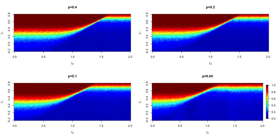
Refer to caption
Figure 8: Empirical detection boundary for random graphs following Erdös-Rényi model with 500 nodes and probability of edge inclusion at 0.4, 0.2, 0.1 and 0.01 respectively.

We also conducted similar experiments for the star graph and cycle graph, each with n=50,250,500n=50,250,500 or 10001000 nodes. The result, as shown in Figures 9 and 10, again agrees well with our theoretical findings.

Refer to caption
Figure 9: Empirical detection boundary for star graph with 50, 250, 500 and 1000 nodes.
Refer to caption
Figure 10: Empirical detection boundary for cycle graph with 50, 250, 500 and 1000 nodes.

5.2 Comparison with other test statistics

To further demonstrate the merits of our method, we now compare the performance of TmaxT_{\max} based test with those based on several other commonly used statistics for gene set enrichment analysis: the maxmean statistic proposed by Efron and Tibshirani (2007); the mean of absolute values; and the χ2\chi^{2} statistic or the mean squares of the scores. To mimic realistic pathways, we simulated signals on three KEGG pathways: hsa00051 with 3333 genes, hsa00140 with 5858 genes, and hsa00230 with 176176 genes. The three pathways were chosen to better illustrate the potential effect of the number of genes, and therefore compliment our asymptotic results. In addition, they are also among the pathways of interest in the NPC data example we shall present later. Detailed pathway information is accessible at http://www.genome.jp. For each pathway, as before, we simulated signal 𝝁\mu such that ‖𝝁‖2=nξ1\|\mbox{\boldmath$\mu$}\|^{2}=n^{\xi_{1}} and 𝝁⊤​L​𝝁=nξ2\mbox{\boldmath$\mu$}^{\top}L\mbox{\boldmath$\mu$}=n^{\xi_{2}} where nn is the number of genes on the pathway and LL is the corresponding Laplacian. We calibrate the null distribution for each test statistic through 1000 Monte Carlo simulations. For each combination of (ξ1,ξ2)(\xi_{1},\xi_{2}), we repeated the experiment in the same fashion for 500 times as before. The power of the test based on each test statistic is given in Figures 11, 12 and 13 for each of the three pathways respectively. It is clear from these results that the TmaxT_{\max} enjoys superior performance than the alternatives under all three settings.

Refer to caption
Figure 11: Power comparison between different tests for signals simulated on pathway hsa00051.
Refer to caption
Figure 12: Power comparison between different tests for signals simulated on pathway hsa00140.
Refer to caption
Figure 13: Power comparison between different tests for signals simulated on pathway hsa00230.

5.3 NPC data example

Our final example is taken from a genome-wide expression study of nasopharyngeal carcinoma (NPC) (Sengupta et al. 2006). The goal of this study is to evaluate the association between host genes in NPC and a key gene in the infecting Epstein-Barr virus (EBV). The data, available from allez package in R, has a total of 4234642346 annotated probe sets. Following Newton et al. (2007) and Newton and Wang (2015), a log-transformed Spearman correlation between viral gene EBNA1 and each human gene was used to evaluate the potential relationship between the viral gene and host genes. Six different gene set enrichment analysis methods were applied to this dataset: in addition to the four test statistics we considered before, Gene set enrichment analysis (GSEA) proposed by Subramanian et al. (2005) was also applied to these scores, as well as the absolute value of these scores. We extracted pathway information for Homo sapiens (org code:hsa) in KEGG, leading to a collection of 301 pathways. We ignored genes on a particular pathway if they are not in our annotated probe sets. For each method, permutation test was applied to determine the pp-value. To adjust for multiple comparison, we applied Benjamini-Hochberg procedure to control the false discovery rate at 0.1%. The pathways that are identified by each method are given in Table 1.

Method Pathways
TmaxT_{\max} hsa03013, hsa03030, hsa03040, hsa03430, hsa04010, hsa04014, hsa04020, hsa04024, hsa04060, hsa04062, hsa04064, hsa04110, hsa04514, hsa04612, hsa04620, hsa04630, hsa04640, hsa04650, hsa04660, hsa04662, hsa04664, hsa04713, hsa04740, hsa04744, hsa05166, hsa05169
MeanAbs hsa03013, hsa03030, hsa03040, hsa03430, hsa04110, hsa04114, hsa04612, hsa04640, hsa04650, hsa04660, hsa05169, hsa05340
Maxmean hsa02010, hsa03008, hsa03013, hsa03030, hsa03040, hsa03430, hsa04020, hsa04060, hsa04062, hsa04064, hsa04080, hsa04110, hsa04261, hsa04380, hsa04514, hsa04612, hsa04630, hsa04640, hsa04650, hsa04660, hsa04662, hsa04672, hsa04713, hsa04740, hsa04925, hsa04940, hsa04970, hsa05320, hsa05321, hsa05330, hsa05332, hsa05340, hsa05414
χ2\chi^{2} hsa03013, hsa03030, hsa03430, hsa04110, hsa04114, hsa04612, hsa04640, hsa04650, hsa04660, hsa05166, hsa05169
GSEA hsa00020, hsa00240, hsa00970, hsa00980, hsa03008, hsa03010, hsa03013, hsa03015, hsa03018, hsa03020, hsa03030, hsa03040, hsa03050, hsa03060, hsa03420, hsa03430, hsa04010, hsa04020, hsa04060, hsa04062, hsa04064, hsa04080, hsa04110, hsa04142, hsa04380, hsa04514, hsa04610, hsa04611, hsa04620, hsa04640, hsa04650, hsa04660, hsa04662, hsa04672, hsa04713, hsa04720, hsa04723, hsa04724, hsa04740, hsa04742, hsa04750, hsa04921, hsa04940, hsa04950, hsa04976, hsa05033, hsa05204, hsa05320, hsa05330, hsa05332, hsa05340, hsa05414
GSEAAbs hsa03013, hsa03030, hsa03040, hsa03430, hsa04110, hsa04612, hsa04640, hsa04650, hsa04940, hsa05320, hsa05330, hsa05332, hsa05340
Table 1: Pathways identified by each method with false discovery rate controlled at 1%.

To gain insights into the reliability of the lists of the pathways identified, we conducted another set of simulation to investigate the operating characteristics of these methods in a setting similar to the NPC data example. To this end, we simulated 4234642346 scores to mimic the NPC data. Each score was simulated from a normal distribution with variance σ2=1.472\sigma^{2}=1.47^{2}, which is the variance estimated from the NPC data. If a gene is not on any of the 26 pathways identified by the proposed method, its mean is set to zero. The means for genes on a pathway with Laplacian LL, we fixed their mean as the same as a smoothed version of the observed scores from the NPC data:

(I+λ​L)−1​𝐱,(I+\lambda L)^{-1}{\bf x},

where 𝐱{\bf x} is the vector of observed scores for genes on the pathway from the NPC data, and λ\lambda is taken to be the tuning parameter that maximizes TλT_{\lambda}. If a gene appears on multiple pathways, we average the means obtained from these pathways. We repeated the experiment for 1000 times and each time, we ran each of the six methods and recorded the lists of pathways they identified to have p-value smaller than 0.1%. The power of each method, along with their false positive ratio, is summarized in Table 2.

graph maxmean absmean chisq gsea gseaabs
hsa03013 0.989 1 0.889 0.877 0.994 0.374
hsa03030 0.889 0.998 0.837 0.889 0.954 0.724
hsa03040 1 1 1 1 0.973 0.81
hsa03430 0.539 0.983 0.595 0.539 0.91 0.657
hsa04010 0.974 1 0.314 0.216 0.825 0.037
hsa04014 0.807 0.998 0.068 0.079 0.713 0.005
hsa04020 0.854 1 0.657 0.486 0.968 0.227
hsa04024 0.856 0.998 0.219 0.142 0.868 0.061
hsa04060 0.999 1 0.962 0.96 1 0.723
hsa04062 0.998 1 0.336 0.307 0.989 0.116
hsa04064 0.745 0.946 0.289 0.43 0.632 0.048
hsa04110 0.995 1 0.51 0.489 0.941 0.123
hsa04514 0.978 1 0.898 0.875 0.938 0.258
hsa04612 0.999 0.989 0.944 0.951 0.276 0.358
hsa04620 0.839 0.829 0.084 0.087 0.867 0.058
hsa04630 1 1 0.349 0.552 0.97 0.035
hsa04640 0.98 1 0.975 0.98 0.94 0.578
hsa04650 0.998 1 0.485 0.733 0.998 0.287
hsa04660 0.861 0.989 0.263 0.246 0.59 0.016
hsa04662 0.845 0.825 0.185 0.182 0.448 0.046
hsa04664 0.444 0.883 0.057 0.069 0.402 0.023
hsa04713 0.994 0.978 0.247 0.086 0.588 0.008
hsa04740 0.926 0.997 0.353 0.313 0.995 0.364
hsa04744 0.536 0.7 0.099 0.084 0.415 0.194
hsa05166 0.848 0.924 0.744 0.653 0.257 0.176
hsa05169 0.998 0.33 0.985 0.985 0.042 0.57
False positive ratio 0.075 0.186 0.027 0.030 0.0790.079 0.0150.015
Table 2: Comparison of power and false positive ratio between different methods based 1000 simulated datasets.

6 Proofs

Proof of Theorem 1.

The main idea of the proof is to identify a set of carefully chosen 𝝁\mus from ΘG​(η2)\Theta_{G}(\eta^{2}) such that ‖𝝁‖2≥c​|V|1/2\|\mbox{\boldmath$\mu$}\|^{2}\geq c|V|^{1/2}, and show that we can not distinguish them collectively from 𝟎{\bf 0}. To this end, denote by 𝐮∈{±1}|V|\mathbf{u}\in\{\pm 1\}^{|V|} a vector of independent Rademacher random variables such that ℙ⁡(ui=+1)=ℙ⁡(ui=−1)=1/2\mathbb{P}(u_{i}=+1)=\mathbb{P}(u_{i}=-1)=1/2. It is clear that

𝔼⁡[𝐮⊤​L​𝐮]=trace⁡(L).\mathbb{E}[\mathbf{u}^{\top}L\mathbf{u}]=\mathrm{trace}(L).

Hereafter we write LL for L⁡(G)L(G) for short when no confusion occurs. By Hanson-Wright inequality (Hanson and Wright, 1971), there exists a constant C>0C>0 such that

ℙ{|𝐮⊤L𝐮−trace(L)|≥t[trace(L)]}≤2exp(−Cmin{t2​[trace⁡(L)]2‖L‖F2,t⁡[trace⁡(L)]‖L‖}).\mathbb{P}\left\{|\mathbf{u}^{\top}L\mathbf{u}-\mathrm{trace}(L)|\geq t[\mathrm{trace}(L)]\right\}\leq 2\exp\left(-C\min\left\{{t^{2}[\mathrm{trace}(L)]^{2}\over\|L\|_{\rm F}^{2}},{t[\mathrm{trace}(L)]\over\|L\|}\right\}\right).

In what follows, we shall use CC to denote a generic positive constant that may take different values at each appearance. Note that LL is a positive semidefinite matrix. Therefore,

‖L‖F2≤[trace⁡(L)]2,and‖L‖≤trace⁡(L).\|L\|_{\rm F}^{2}\leq[\mathrm{trace}(L)]^{2},\qquad{\rm and}\qquad\|L\|\leq\mathrm{trace}(L).

For any t≥1t\geq 1, we get

ℙ{𝐮⊤L𝐮≤(t+1)trace(L)}≥1−exp(−Ct).\mathbb{P}\left\{\mathbf{u}^{\top}L\mathbf{u}\leq(t+1)\mathrm{trace}(L)\right\}\geq 1-\exp(-Ct).

Because scaling does not change the rates of detection, we can assume without loss of generality that η2>ηmax2​(G)\eta^{2}>\eta_{\max}^{2}(G). Then

ℙ{|V|−1/2𝐮⊤L𝐮≤η2}≥1−exp(−Cη2/ηmax2).\mathbb{P}\left\{|V|^{-1/2}\mathbf{u}^{\top}L\mathbf{u}\leq\eta^{2}\right\}\geq 1-\exp(-C\eta^{2}/\eta_{\max}^{2}).

Denote by 𝒰\mathcal{U} the collection of all 𝐮∈{±1}|V|\mathbf{u}\in\{\pm 1\}^{|V|} such that

𝐮⊤​L​𝐮≤|V|1/2​η2.\mathbf{u}^{\top}L\mathbf{u}\leq|V|^{1/2}\eta^{2}.

Then

|𝒰|≥[1−exp(−Cη2/ηmax2)]2|V|.|\mathcal{U}|\geq\left[1-\exp(-C\eta^{2}/\eta_{\max}^{2})\right]2^{|V|}.

Let ℙ𝝁\mathbb{P}_{\mbox{\boldmath$\mu$}} be the probability measure of (Xv)v∈V(X_{v})_{v\in V} such that Xv∼N⁡(μv,1)X_{v}\sim N(\mu_{v},1). Write

ℙ1=1|𝒰|∑𝐮∈𝒰ℙζ|V|−1/4𝐮,\mathbb{P}_{1}={1\over|\mathcal{U}|}\sum_{\mathbf{u}\in\mathcal{U}}\mathbb{P}_{\zeta|V|^{-1/4}\mathbf{u}},

for some 0≤ζ≤10\leq\zeta\leq 1 to be specified later. Then for any test ϕ\phi, the sum of the probabilities of its two types of errors obeys

sup𝐮∈𝒰{𝔼0ϕ+𝔼|V|−1/4𝐮(1−ϕ)}\displaystyle\sup_{\mathbf{u}\in\mathcal{U}}\left\{\mathbb{E}_{0}\phi+\mathbb{E}_{|V|^{-1/4}\mathbf{u}}(1-\phi)\right\} ≥\displaystyle\geq infψsup𝐮∈𝒰{𝔼0ψ+𝔼|V|−1/4𝐮(1−ψ)}\displaystyle\inf_{\psi}\sup_{\mathbf{u}\in\mathcal{U}}\left\{\mathbb{E}_{0}\psi+\mathbb{E}_{|V|^{-1/4}\mathbf{u}}(1-\psi)\right\}
≥\displaystyle\geq infψ1|𝒰|∑𝐮∈𝒰{𝔼0ψ+𝔼|V|−1/4𝐮(1−ψ)}\displaystyle\inf_{\psi}{1\over|\mathcal{U}|}\sum_{\mathbf{u}\in\mathcal{U}}\left\{\mathbb{E}_{0}\psi+\mathbb{E}_{|V|^{-1/4}\mathbf{u}}(1-\psi)\right\}
=\displaystyle= 1−12​‖ℙ0−ℙ1‖ℓ1.\displaystyle 1-{1\over 2}\|\mathbb{P}_{0}-\mathbb{P}_{1}\|_{\ell_{1}}.

Recall that

‖ℙ0−ℙ1‖ℓ12≤∫f12f0−1,\|\mathbb{P}_{0}-\mathbb{P}_{1}\|_{\ell_{1}}^{2}\leq\int{f_{1}^{2}\over f_{0}}-1,

where f1f_{1} and f0f_{0} are the density functions corresponding to ℙ0\mathbb{P}_{0} and ℙ1\mathbb{P}_{1} respectively.

It is not hard to see that

∫f12f0\displaystyle\int{f_{1}^{2}\over f_{0}} =\displaystyle= 1|𝒰|2∑𝐮1,𝐮2∈𝒰exp(ζ2|V|−1/2𝐮1⊤𝐮2)\displaystyle{1\over|\mathcal{U}|^{2}}\sum_{\mathbf{u}_{1},\mathbf{u}_{2}\in\mathcal{U}}\exp(\zeta^{2}|V|^{-1/2}\mathbf{u}_{1}^{\top}\mathbf{u}_{2})
≤\displaystyle\leq 1|𝒰|2∑𝐮1,𝐮2∈{±1}|V|exp(ζ2|V|−1/2𝐮1⊤𝐮2)\displaystyle{1\over|\mathcal{U}|^{2}}\sum_{\mathbf{u}_{1},\mathbf{u}_{2}\in\{\pm 1\}^{|V|}}\exp(\zeta^{2}|V|^{-1/2}\mathbf{u}_{1}^{\top}\mathbf{u}_{2})
≤\displaystyle\leq [1−exp(−Cη2/ηmax2)]−2𝔼exp(ζ2|V|−1/2𝐮1⊤𝐮2),\displaystyle\left[1-\exp(-C\eta^{2}/\eta_{\max}^{2})\right]^{-2}\mathbb{E}\exp(\zeta^{2}|V|^{-1/2}\mathbf{u}_{1}^{\top}\mathbf{u}_{2}),

where the expectation is taken over two independent Radmacher random vectors 𝐮1\mathbf{u}_{1} and 𝐮2\mathbf{u}_{2}. Note that

𝔼exp(ζ2|V|−1/2𝐮1⊤𝐮2)=𝔼exp[ζ2|V|−1/2(2B−1)],\mathbb{E}\exp(\zeta^{2}|V|^{-1/2}\mathbf{u}_{1}^{\top}\mathbf{u}_{2})=\mathbb{E}\exp[\zeta^{2}|V|^{-1/2}(2B-1)],

where B∼Bin⁡(|V|,1/2)B\sim{\rm Bin}(|V|,1/2). By Central Limit Theorem,

𝔼exp[ζ2|V|−1/2(2B−1)]→exp(ζ4/2).\mathbb{E}\exp[\zeta^{2}|V|^{-1/2}(2B-1)]\to\exp(\zeta^{4}/2).

Therefore, when |V||V| is large enough, for any test ϕ\phi,

sup𝐮∈𝒰{𝔼0ϕ+𝔼|V|−1/4𝐮(1−ϕ)}\displaystyle\sup_{\mathbf{u}\in\mathcal{U}}\left\{\mathbb{E}_{0}\phi+\mathbb{E}_{|V|^{-1/4}\mathbf{u}}(1-\phi)\right\} ≥\displaystyle\geq 1−12[1−exp(−Cη2/ηmax2)]−2exp⁡(ζ4/2)−1\displaystyle 1-{1\over 2}\left[1-\exp(-C\eta^{2}/\eta_{\max}^{2})\right]^{-2}\sqrt{\exp(\zeta^{4}/2)-1}
≥\displaystyle\geq 1−ζ22[1−exp(−Cη2/ηmax2)]−2,\displaystyle 1-{\zeta^{2}\over 2}\left[1-\exp(-C\eta^{2}/\eta_{\max}^{2})\right]^{-2},

where in the second inequality we used the fact that ex≤1+2​xe^{x}\leq 1+2x for any x<1/2x<1/2. The desired claim then follows from the fact that ∥ζ|V|−1/4𝐮∥2=ζ2|V|1/2\|\zeta|V|^{-1/4}\mathbf{u}\|^{2}=\zeta^{2}|V|^{1/2}. ∎

Proof of Theorem 2.

Denote by P0P_{0} the projection matrix from ℝ|V|\mathbb{R}^{|V|} to the eigenspace of L⁡(G)L(G) corresponding to eigenvalue zero. It is not hard to see that, if 𝐗∼N⁡(𝝁,I)\mathbf{X}\sim N(\mbox{\boldmath$\mu$},I), then

R∼χK2​(‖P0​𝝁‖2).R\sim\chi^{2}_{K}(\|P_{0}\mbox{\boldmath$\mu$}\|^{2}).

Observe that

𝝁⊤​L​(G)​𝝁≥ηmin2​(G)​‖P0⟂​𝝁‖2,\mbox{\boldmath$\mu$}^{\top}L(G)\mbox{\boldmath$\mu$}\geq\eta_{\min}^{2}(G)\|P_{0}^{\perp}\mbox{\boldmath$\mu$}\|^{2},

so that

‖P0⟂​𝝁‖2≤η2/ηmin2​(G).\|P_{0}^{\perp}\mbox{\boldmath$\mu$}\|^{2}\leq\eta^{2}/\eta_{\min}^{2}(G).

Therefore,

‖P0​𝝁‖2=‖𝝁‖2−‖P0⟂​𝝁‖2≥‖𝝁‖2−η2/ηmin2​(G),\|P_{0}\mbox{\boldmath$\mu$}\|^{2}=\|\mbox{\boldmath$\mu$}\|^{2}-\|P_{0}^{\perp}\mbox{\boldmath$\mu$}\|^{2}\geq\|\mbox{\boldmath$\mu$}\|^{2}-\eta^{2}/\eta_{\min}^{2}(G),

which is of the same order as ‖𝝁‖2\|\mbox{\boldmath$\mu$}\|^{2} if ‖𝝁‖2≫η2/ηmin2​(G)\|\mbox{\boldmath$\mu$}\|^{2}\gg\eta^{2}/\eta_{\min}^{2}(G). The proof is then completed. ∎

Proof of Theorem 3.

We first note that an Erdös-Rényi graph GnG_{n} is connected with probability tending to one suggesting that its Laplacian L⁡(Gn)L(G_{n}) has exactly one zero eigenvalue. Recall that L⁡(Gn)=D⁡(Gn)−A⁡(Gn)L(G_{n})=D(G_{n})-A(G_{n}) where D⁡(Gn)D(G_{n}) and A⁡(Gn)A(G_{n}) are GnG_{n}’s degree and adjacency matrices respectively. Applying random matrix theory, Füredi and Komlós (1981) showed that the eigenvalues of A⁡(Gn)A(G_{n}) are Op​(n​p)O_{p}(\sqrt{np}) with the exception of the largest one. On the other hand, by Chernoff’s bound, ‖D⁡(Gn)−n​p‖=Op​(n​p)\|D(G_{n})-np\|=O_{p}(\sqrt{np}). Thus, all nonzero eigenvalues of L⁡(Gn)L(G_{n}) are n​p+Op​(n​p)np+O_{p}(\sqrt{np}). In other words, we can write

L⁡(Gn)=J+Δ,L(G_{n})=J+\Delta,

where

J=(n​p)​(I−1n​𝟏𝟏⊤),J=(np)\left(I-{1\over n}\mathbf{1}\mathbf{1}^{\top}\right),

and Δ\Delta is a symmetric matrix such that Δ​𝟏=𝟎\Delta\mathbf{1}=\mathbf{0} and ‖Δ‖=Op​(n​p)\|\Delta\|=O_{p}(\sqrt{np}).

Observe that

𝐗⊤​(I+α​L​(Gn))−1​𝐗\displaystyle\mathbf{X}^{\top}(I+\alpha L(G_{n}))^{-1}\mathbf{X} =\displaystyle= 𝐗⊤(I+αJ)−1[I+α(I+αJ)−1Δ)]−1𝐗\displaystyle\mathbf{X}^{\top}(I+\alpha J)^{-1}\left[I+\alpha(I+\alpha J)^{-1}\Delta)\right]^{-1}\mathbf{X}
=\displaystyle= 𝐗⊤​(I+α​J)−1​𝐗⋅[1+O⁡((n​p)−1​‖Δ‖)].\displaystyle\mathbf{X}^{\top}(I+\alpha J)^{-1}\mathbf{X}\cdot[1+O\left((np)^{-1}\|\Delta\|\right)].

Similarly, we can show that

trace⁡[(I+α​L​(Gn))−1]=trace⁡[(I+α​J)−1]⋅[1+O⁡((n​p)−1​‖Δ‖)],\mathrm{trace}[(I+\alpha L(G_{n}))^{-1}]=\mathrm{trace}[(I+\alpha J)^{-1}]\cdot[1+O\left((np)^{-1}\|\Delta\|\right)],

and

{trace⁡[(I+α​L​(Gn))−2]}1/2={trace⁡[(I+α​J)−2]}1/2⋅[1+O⁡((n​p)−1​‖Δ‖)].\left\{\mathrm{trace}[(I+\alpha L(G_{n}))^{-2}]\right\}^{1/2}=\left\{\mathrm{trace}[(I+\alpha J)^{-2}]\right\}^{1/2}\cdot[1+O\left((np)^{-1}\|\Delta\|\right)].

Therefore

Tα=𝐗⊤​(I+α​J)−1​𝐗−trace⁡[(I+α​J)−1]{trace⁡[(I+α​J)−2]}1/2⋅[1+O⁡((n​p)−1​‖Δ‖)],T_{\alpha}={\mathbf{X}^{\top}(I+\alpha J)^{-1}\mathbf{X}-\mathrm{trace}[(I+\alpha J)^{-1}]\over\left\{\mathrm{trace}[(I+\alpha J)^{-2}]\right\}^{1/2}}\cdot[1+O\left((np)^{-1}\|\Delta\|\right)],

which implies that

Tmax=maxα≥0Tα=maxα≥0{𝐗⊤​(I+α​J)−1​𝐗−trace⁡[(I+α​J)−1]{trace⁡[(I+α​J)−2]}1/2}⋅[1+Op((np)−1/2)].T_{\max}=\max_{\alpha\geq 0}T_{\alpha}=\max_{\alpha\geq 0}\left\{{\mathbf{X}^{\top}(I+\alpha J)^{-1}\mathbf{X}-\mathrm{trace}[(I+\alpha J)^{-1}]\over\left\{\mathrm{trace}[(I+\alpha J)^{-2}]\right\}^{1/2}}\right\}\cdot[1+O_{p}((np)^{-1/2})]. (18)

On the other hand,

𝐗⊤​(I+α​J)−1​𝐗−trace⁡[(I+α​J)−1]{trace⁡[(I+α​J)−2]}1/2\displaystyle{\mathbf{X}^{\top}(I+\alpha J)^{-1}\mathbf{X}-\mathrm{trace}[(I+\alpha J)^{-1}]\over\left\{\mathrm{trace}[(I+\alpha J)^{-2}]\right\}^{1/2}}
=\displaystyle= (n−1(1+n​p​α)2+1)−1/2{11+n​p​α⋅[∥𝐱c∥2−(n−1)]+(nx¯2−1)}.\displaystyle\left({n-1\over(1+np\alpha)^{2}}+1\right)^{-1/2}\left\{{1\over 1+np\alpha}\cdot\left[\|\mathbf{x}_{c}\|^{2}-(n-1)\right]+(n\bar{x}^{2}-1)\right\}.

Thus,

maxα≥0{𝐗⊤​(I+α​J)−1​𝐗−trace⁡[(I+α​J)−1]{trace⁡[(I+α​J)−2]}1/2}=maxθ∈[n−1/2,1]{1−θ2⋅W1+θ⋅W2},\max_{\alpha\geq 0}\left\{{\mathbf{X}^{\top}(I+\alpha J)^{-1}\mathbf{X}-\mathrm{trace}[(I+\alpha J)^{-1}]\over\left\{\mathrm{trace}[(I+\alpha J)^{-2}]\right\}^{1/2}}\right\}=\max_{\theta\in[n^{-1/2},1]}\left\{\sqrt{1-\theta^{2}}\cdot W_{1}+\theta\cdot W_{2}\right\},

where

W1=1n−1​[‖𝐱c‖2−(n−1)],andW2=n​x¯2−1.W_{1}={1\over\sqrt{n-1}}\left[\|\mathbf{x}_{c}\|^{2}-(n-1)\right],\qquad{\rm and}\qquad W_{2}=n\bar{x}^{2}-1.

Write

h⁡(θ)=1−θ2⋅W1+θ⋅W2.h(\theta)=\sqrt{1-\theta^{2}}\cdot W_{1}+\theta\cdot W_{2}.

It is clear that

h′​(θ)=W2−θ1−θ2⋅W1.h^{\prime}(\theta)=W_{2}-{\theta\over\sqrt{1-\theta^{2}}}\cdot W_{1}.

By first order condition, we get

maxθ∈[n−1/2,1]h(θ)={(W12+W22)1/2if​W1,W2>0max⁡{W1,W2}otherwise\max_{\theta\in[n^{-1/2},1]}h(\theta)=\left\{\begin{array}[]{ll}(W_{1}^{2}+W_{2}^{2})^{1/2}&{\rm if\ }W_{1},W_{2}>0\\ \max\left\{W_{1},W_{2}\right\}&{\rm otherwise}\end{array}\right.

It is not hard to see that

W1→dN(2δ12,2),andW2→dχ12(δ22)−1.W_{1}\to_{d}N(\sqrt{2}\delta_{1}^{2},2),\qquad{\rm and}\qquad W_{2}\to_{d}\chi^{2}_{1}(\delta_{2}^{2})-1.

This, together with (18), implies (9). ∎

Proof of Theorem 4.

By Theorem 3, φ\varphi is consistent for testing against any effect 𝝁\mu such that

1n1/2​‖𝝁c‖2+n​μ¯2→∞,asn→∞.{1\over n^{1/2}}\|\mbox{\boldmath$\mu$}_{c}\|^{2}+n\bar{\mu}^{2}\to\infty,\qquad{\rm as}\quad n\to\infty. (19)

In addition, as shown in the proof of Theorem 3,

L⁡(Gn)=(n​p)​J+ΔL(G_{n})=(np)J+\Delta

such that Δ​𝟏=𝟎\Delta\mathbf{1}=\mathbf{0} and ‖Δ‖=Op​(n​p)\|\Delta\|=O_{p}(\sqrt{np}). Thus,

𝝁⊤​L​(Gn)​𝝁=(n​p)​𝝁⊤​J​𝝁+Op​(‖𝝁c‖2​n​p)=‖𝝁c‖2​(n​p+Op​(n​p)),\mbox{\boldmath$\mu$}^{\top}L(G_{n})\mbox{\boldmath$\mu$}=(np)\mbox{\boldmath$\mu$}^{\top}J\mbox{\boldmath$\mu$}+O_{p}(\|\mbox{\boldmath$\mu$}_{c}\|^{2}\sqrt{np})=\|\mbox{\boldmath$\mu$}_{c}\|^{2}(np+O_{p}(\sqrt{np})),

which implies that ‖𝝁c‖2≫n1/2\|\mbox{\boldmath$\mu$}_{c}\|^{2}\gg n^{1/2} if η2≫n3/2\eta^{2}\gg n^{3/2}. Together with the fact that

‖𝝁‖2=‖𝝁c‖2+n​μ¯2,\|\mbox{\boldmath$\mu$}\|^{2}=\|\mbox{\boldmath$\mu$}_{c}\|^{2}+n\bar{\mu}^{2},

this immediately implies that when η2≫n3/2\eta^{2}\gg n^{3/2}, β⁡(φ,𝝁)→0\beta(\varphi;\mbox{\boldmath$\mu$})\to 0 if ‖𝝁‖2≫n1/2\|\mbox{\boldmath$\mu$}\|^{2}\gg n^{1/2}; and on the other hand, when η2=O⁡(n3/2)\eta^{2}=O(n^{3/2}), β⁡(φ,𝝁)→0\beta(\varphi;\mbox{\boldmath$\mu$})\to 0 if ‖𝝁‖2=η2/n+ω⁡(1)\|\mbox{\boldmath$\mu$}\|^{2}=\eta^{2}/n+\omega(1). This completes the proof of the first statement.

We now show that this indeed is the best one can do. Note that

trace⁡(L⁡(Gn))=n⁡(n−1)​p​(1+op​(1)).\mathrm{trace}(L(G_{n}))=n(n-1)p(1+o_{p}(1)).

The lower bound for the case when η2=Ω⁡(n3/2)\eta^{2}=\Omega(n^{3/2}) then follows immediately from Theorem 1. Similarly, the lower bound for the case when η=O⁡(n1/2)\eta=O(n^{1/2}) follows from Theorem 2 since the minimum nonzero eigenvalue of L⁡(Gn)L(G_{n}) is of the form n​p+Op​(n​p)np+O_{p}(\sqrt{np}). It remains to treat the case when n1/2≪η≪n3/4n^{1/2}\ll\eta\ll n^{3/4}.

To this end, let 𝐰1,…,𝐰n−1\mathbf{w}_{1},\ldots,\mathbf{w}_{n-1} be an (arbitrary) orthogonal basis of the linear subspace

{𝐱∈ℝ|V|:𝐱⊤​𝟏=𝟎}.\{\mathbf{x}\in\mathbb{R}^{|V|}:\mathbf{x}^{\top}\mathbf{1}=\mathbf{0}\}.

Write k∗=⌊η4/n2⌋k_{\ast}=\lfloor\eta^{4}/n^{2}\rfloor. For any 𝐮∈{±1}k∗\mathbf{u}\in\{\pm 1\}^{k_{\ast}}, denote by ℙ𝐮\mathbb{P}_{\mathbf{u}} the probability measure of 𝐗=(Xv)v∈V\mathbf{X}=(X_{v})_{v\in V} such that 𝐗∼N⁡(𝝁,In)\mathbf{X}\sim N(\mbox{\boldmath$\mu$},I_{n}), where

𝝁=ζη(nk∗)−1/2∑k=1k∗uk𝐰k,\mbox{\boldmath$\mu$}=\zeta\eta(nk_{\ast})^{-1/2}\sum_{k=1}^{k_{\ast}}u_{k}\mathbf{w}_{k}, (20)

for some ζ<1\zeta<1 to be specified later. It is not hard to see that, with this choice,

𝝁⊤​L​(Gn)​𝝁=ζ2​η2​(n​k∗)−1​∑k=1k∗λk​(Gn)=ζ2​η2​p​(1+op​(1)),\mbox{\boldmath$\mu$}^{\top}L(G_{n})\mbox{\boldmath$\mu$}=\zeta^{2}\eta^{2}(nk_{\ast})^{-1}\sum_{k=1}^{k_{\ast}}\lambda_{k}(G_{n})=\zeta^{2}\eta^{2}p(1+o_{p}(1)),

indicating 𝝁∈ΘGn​(η2)\mbox{\boldmath$\mu$}\in\Theta_{G_{n}}(\eta^{2}) with probability tending to one. As before, denote by 𝒰\mathcal{U} the collection of 𝐮\mathbf{u} such that the corresponding 𝝁\mu as defined by (20) belongs to ΘGn​(η2)\Theta_{G_{n}}(\eta^{2}). Then |𝒰|/2k∗→p1|\mathcal{U}|/2^{k_{\ast}}\to_{p}1. Write

ℙ1=1|𝒰|​∑𝐮∈𝒰ℙ𝐮.\mathbb{P}_{1}={1\over|\mathcal{U}|}\sum_{\mathbf{u}\in\mathcal{U}}\mathbb{P}_{\mathbf{u}}.

Following the same calculation as before, it suffices to show that ∫(f12/f0)\int(f_{1}^{2}/f_{0}) can be made arbitrarily close to 11. Recall that

∫f12f0=𝔼​exp⁡[ζ2​η2​(n​k∗)−1​𝐮1⊤​𝐮2],\int{f_{1}^{2}\over f_{0}}=\mathbb{E}\exp[\zeta^{2}\eta^{2}(nk_{\ast})^{-1}\mathbf{u}_{1}^{\top}\mathbf{u}_{2}],

where the expectation is taken over two independent random vectors 𝐮1\mathbf{u}_{1} and 𝐮2\mathbf{u}_{2} uniformly sampled from 𝒰\mathcal{U}. Following a similar argument as that of Theorem 1, we can derive that

𝔼​exp⁡[ζ2​η2​(n​k∗)−1​𝐮1⊤​𝐮2]→exp⁡(ζ4/2).\mathbb{E}\exp[\zeta^{2}\eta^{2}(nk_{\ast})^{-1}\mathbf{u}_{1}^{\top}\mathbf{u}_{2}]\to\exp(\zeta^{4}/2).

By taking ζ\zeta small enough, we can ensure that any test is powerless in testing against 𝝁\mu of the form (20) with 𝐮∈𝒰\mathbf{u}\in\mathcal{U}. The proof is then completed by noting that

‖𝝁‖2≤ζ2​η2n,\|\mbox{\boldmath$\mu$}\|^{2}\leq{\zeta^{2}\eta^{2}\over n},

for any 𝐮∈𝒰\mathbf{u}\in\mathcal{U}. ∎

Proof of Theorem 5.

For brevity, we omit the dependence of the Laplacian matrix LL on GG and write n:=|V|n:=|V| throughout the proof. We first prove the first statement. To this end, let

α∗=arg​maxα⁡{‖H⁡(α)‖F−1​𝝁⊤​H​(α)​𝝁},\alpha_{\ast}=\argmax_{\alpha}\left\{\|H(\alpha)\|_{\rm F}^{-1}\mbox{\boldmath$\mu$}^{\top}H(\alpha)\mbox{\boldmath$\mu$}\right\},

where

H⁡(α)=(I+α​L)−1.H(\alpha)=(I+\alpha L)^{-1}.

Of course, the maximizer may not be unique, in which case, α∗\alpha_{\ast} is chosen arbitrarily among the maximizers. By Hanson-Wright inequality (Hanson and Wright, 1971),

ℙ{|Tα∗−∥H(α∗)∥F−1𝝁⊤H(α∗)𝝁|≥t}≤2exp(−Cmin{t2,t∥H(α∗)∥F}),\mathbb{P}\left\{|T_{\alpha_{\ast}}-\|H(\alpha_{\ast})\|_{\rm F}^{-1}\mbox{\boldmath$\mu$}^{\top}H(\alpha_{\ast})\mbox{\boldmath$\mu$}|\geq t\right\}\leq 2\exp\left(-C\min\left\{t^{2},{t\|H(\alpha_{\ast})\|_{\rm F}}\right\}\right),

This immediately implies that

ℙ{Tα∗≤12∥H(α∗)∥F−1𝝁⊤H(α∗)𝝁}≤2exp(−Cmin{∥H(α∗)∥F−2(𝝁⊤H(α∗)𝝁)2,𝝁⊤H(α∗)𝝁}).\mathbb{P}\left\{T_{\alpha_{\ast}}\leq{1\over 2}\|H(\alpha_{\ast})\|_{\rm F}^{-1}\mbox{\boldmath$\mu$}^{\top}H(\alpha_{\ast})\mbox{\boldmath$\mu$}\right\}\leq 2\exp\left(-C\min\left\{\|H(\alpha_{\ast})\|_{\rm F}^{-2}\left(\mbox{\boldmath$\mu$}^{\top}H(\alpha_{\ast})\mbox{\boldmath$\mu$}\right)^{2},\mbox{\boldmath$\mu$}^{\top}H(\alpha_{\ast})\mbox{\boldmath$\mu$}\right\}\right).

It is therefore clear that

Tmax≥Tα∗≫log⁡log⁡n,T_{\max}\geq T_{\alpha_{\ast}}\gg\log\log n,

with probability tending to one, by assumption (12). It now suffices to show that under H0H_{0},

Tmax=Op​(log⁡log⁡n).T_{\max}=O_{p}(\log\log n).

With slight abuse of notation, let 0=ρ0<ρ1<⋯<ρN0=\rho_{0}<\rho_{1}<\cdots<\rho_{N} be the distinct eigenvalues of LL and nkn_{k} be the multiplicity of ρk\rho_{k}. Write 𝐰α=(wα,1,…,wα,N)⊤\mathbf{w}_{\alpha}=(w_{\alpha,1},\ldots,w_{\alpha,N})^{\top} where

wα,k=nk1+α​ρk,k=0,1,…,N.w_{\alpha,k}={\sqrt{n_{k}}\over 1+\alpha\rho_{k}},\qquad k=0,1,\ldots,N.

Then, under H0H_{0}, TmaxT_{\max} follows the same distribution as

supα≥0{‖𝐰α‖−1​∑k=0Nwα,k​Yk},\sup_{\alpha\geq 0}\left\{\|\mathbf{w}_{\alpha}\|^{-1}\sum_{k=0}^{N}w_{\alpha,k}Y_{k}\right\},

where Yk∼nk−1/2(χnk2−nk)Y_{k}\sim n_{k}^{-1/2}(\chi^{2}_{n_{k}}-n_{k}), k=0,1,…,Nk=0,1,\ldots,N, are independent random variables. Note that for any 0<αmin<αmax<∞0<\alpha_{\min}<\alpha_{\max}<\infty,

supα≥0{‖𝐰α‖−1​∑k=0Nwα,k​Yk}\displaystyle\sup_{\alpha\geq 0}\left\{\|\mathbf{w}_{\alpha}\|^{-1}\sum_{k=0}^{N}w_{\alpha,k}Y_{k}\right\}
=\displaystyle= max{supα∈[0,αmin]{∥𝐰α∥−1∑k=0Nwα,kYk},supα∈(αmin,αmax){∥𝐰α∥−1∑k=0Nwα,kYk},\displaystyle\max\biggl\{\sup_{\alpha\in[0,\alpha_{\min}]}\{\|\mathbf{w}_{\alpha}\|^{-1}\sum_{k=0}^{N}w_{\alpha,k}Y_{k}\},\sup_{\alpha\in(\alpha_{\min},\alpha_{\max})}\{\|\mathbf{w}_{\alpha}\|^{-1}\sum_{k=0}^{N}w_{\alpha,k}Y_{k}\},
supα>αmax{∥𝐰α∥−1∑k=0Nwα,kYk}}\displaystyle\hskip 50.0pt\sup_{\alpha>\alpha_{\max}}\{\|\mathbf{w}_{\alpha}\|^{-1}\sum_{k=0}^{N}w_{\alpha,k}Y_{k}\}\biggr\}

We now treat the three terms on the righthand side separately with appropriately chosen αmin\alpha_{\min} and αmax\alpha_{\max}.

Small α\alphas.

We first consider the case when α\alpha is small in that

α≤αmin:=1[trace⁡(L2)]1/2​log⁡(N+1).\alpha\leq\alpha_{\min}:={1\over[\mathrm{trace}(L^{2})]^{1/2}\log(N+1)}.

Observe that, if α≤αmin\alpha\leq\alpha_{\min}, then α​ρk≤1\alpha\rho_{k}\leq 1 for k=1,…,Nk=1,\ldots,N. Thus,

‖𝐰α‖2=∑k=0Nnk(1+α​ρk)2≥n4.\|\mathbf{w}_{\alpha}\|^{2}=\sum_{k=0}^{N}{n_{k}\over(1+\alpha\rho_{k})^{2}}\geq{n\over 4}.

We then get

supα∈[0,αmin]{‖𝐰α‖−1​∑k=0Nwα,k​Yk}\displaystyle\sup_{\alpha\in[0,\alpha_{\min}]}\left\{\|\mathbf{w}_{\alpha}\|^{-1}\sum_{k=0}^{N}w_{\alpha,k}Y_{k}\right\} ≤\displaystyle\leq ‖𝐰αmin‖−1​(|∑k=0Nnk​Yk|+supα∈[0,αmin]|∑k=0N(wα,k−nk)​Yk|)\displaystyle\|\mathbf{w}_{\alpha_{\min}}\|^{-1}\left(\left|\sum_{k=0}^{N}\sqrt{n_{k}}Y_{k}\right|+\sup_{\alpha\in[0,\alpha_{\min}]}\left|\sum_{k=0}^{N}(w_{\alpha,k}-\sqrt{n_{k}})Y_{k}\right|\right)
≤\displaystyle\leq (4n​|∑k=0Nnk​Yk|+‖𝐰αmin‖−1​supα∈[0,αmin]|∑k=0N(wα,k−nk)​Yk|)\displaystyle\left(\sqrt{4\over n}\left|\sum_{k=0}^{N}\sqrt{n_{k}}Y_{k}\right|+\|\mathbf{w}_{\alpha_{\min}}\|^{-1}\sup_{\alpha\in[0,\alpha_{\min}]}\left|\sum_{k=0}^{N}(w_{\alpha,k}-\sqrt{n_{k}})Y_{k}\right|\right)
≤\displaystyle\leq Op​(1)+‖𝐰αmin‖−1​supα∈[0,αmin]|∑k=0N(wα,k−nk)​Yk|.\displaystyle O_{p}(1)+\|\mathbf{w}_{\alpha_{\min}}\|^{-1}\sup_{\alpha\in[0,\alpha_{\min}]}\left|\sum_{k=0}^{N}(w_{\alpha,k}-\sqrt{n_{k}})Y_{k}\right|.

where the last inequality follows from Markov inequality and the fact that

𝔼​|∑k=0Nnk​Yk|2=∑k=0Nnk​𝔼​Yk2=2​n.\mathbb{E}\left|\sum_{k=0}^{N}\sqrt{n_{k}}Y_{k}\right|^{2}=\sum_{k=0}^{N}n_{k}\mathbb{E}Y_{k}^{2}=2n.

Now note that for any α∈[0,αmin]\alpha\in[0,\alpha_{\min}], α​ρk≤1\alpha\rho_{k}\leq 1 so that

|∑k=0N(wα,k−nk)​Yk|≤(∑k=1Nnk​α​ρk1+α​ρk)​max1≤k≤N​|Yk|.\left|\sum_{k=0}^{N}(w_{\alpha,k}-\sqrt{n_{k}})Y_{k}\right|\leq\left(\sum_{k=1}^{N}{\sqrt{n_{k}}\alpha\rho_{k}\over 1+\alpha\rho_{k}}\right)\max_{1\leq k\leq N}|Y_{k}|.

By Cauchy-Schwartz inequality,

|∑k=0N(wα,k−nk)​Yk|\displaystyle\left|\sum_{k=0}^{N}(w_{\alpha,k}-\sqrt{n_{k}})Y_{k}\right| ≤\displaystyle\leq α​‖𝐰α‖​(∑k=1Nnk​ρk2)1/2​max1≤k≤N​|Yk|\displaystyle\alpha\|\mathbf{w}_{\alpha}\|\left(\sum_{k=1}^{N}n_{k}\rho_{k}^{2}\right)^{1/2}\max_{1\leq k\leq N}|Y_{k}|
=\displaystyle= α​‖𝐰α‖​[trace⁡(L2)]1/2​max1≤k≤N​|Yk|.\displaystyle\alpha\|\mathbf{w}_{\alpha}\|[\mathrm{trace}(L^{2})]^{1/2}\max_{1\leq k\leq N}|Y_{k}|.

By the choice of αmin\alpha_{\min}, together with the fact that

max1≤k≤N⁡|Yk|=Op​(log⁡N),\max_{1\leq k\leq N}|Y_{k}|=O_{p}(\log N),

we get

supα∈[0,αmin]{‖𝐰α‖−1​∑k=0Nwα,k​Yk}=Op​(1).\sup_{\alpha\in[0,\alpha_{\min}]}\left\{\|\mathbf{w}_{\alpha}\|^{-1}\sum_{k=0}^{N}w_{\alpha,k}Y_{k}\right\}=O_{p}(1).

Large α\alphas

Next we consider the case when α\alpha is large in that

α≥αmax:=log⁡(N+1)n0​∑k=1Nnkρk,\alpha\geq\alpha_{\max}:={\log(N+1)\over\sqrt{n_{0}}}\sum_{k=1}^{N}{\sqrt{n_{k}}\over\rho_{k}},

where n0=Kn_{0}=K is the number of connected components of GG.

It is clear that ‖𝐰α‖≥wα,0=n0\|\mathbf{w}_{\alpha}\|\geq w_{\alpha,0}=\sqrt{n_{0}}. Thus,

‖𝐰α‖−1​∑k=0Nwα,k​Yk\displaystyle\|\mathbf{w}_{\alpha}\|^{-1}\sum_{k=0}^{N}w_{\alpha,k}Y_{k} ≤\displaystyle\leq wα,0−1​|∑k=0Nwα,k​Yk|\displaystyle w_{\alpha,0}^{-1}\left|\sum_{k=0}^{N}w_{\alpha,k}Y_{k}\right|
≤\displaystyle\leq |Y0|+wα,0−1​|∑k=1Nwα,k​Yk|\displaystyle|Y_{0}|+w_{\alpha,0}^{-1}\left|\sum_{k=1}^{N}w_{\alpha,k}Y_{k}\right|
≤\displaystyle\leq Op​(1)+wα,0−1​(∑k=1Nwα,k)​max1≤k≤N​|Yk|.\displaystyle O_{p}(1)+w_{\alpha,0}^{-1}\left(\sum_{k=1}^{N}w_{\alpha,k}\right)\max_{1\leq k\leq N}\left|Y_{k}\right|.

Recall that, for any α≥αmax\alpha\geq\alpha_{\max},

∑k=1Nwα,k=∑k=1Nnk1+α​ρk≤∑k=1Nnkα​ρk≤n0log⁡(N+1).\sum_{k=1}^{N}w_{\alpha,k}=\sum_{k=1}^{N}{\sqrt{n_{k}}\over 1+\alpha\rho_{k}}\leq\sum_{k=1}^{N}{\sqrt{n_{k}}\over\alpha\rho_{k}}\leq{\sqrt{n_{0}}\over\log(N+1)}.

Together with the fact that

max1≤k≤N⁡|Yk|=Op​(log⁡N),\max_{1\leq k\leq N}\left|Y_{k}\right|=O_{p}(\log N),

we get

supα≥αmax{‖𝐰α‖−1​∑k=1nwα,k​Yk}=Op​(1).\sup_{\alpha\geq\alpha_{\max}}\left\{\|\mathbf{w}_{\alpha}\|^{-1}\sum_{k=1}^{n}w_{\alpha,k}Y_{k}\right\}=O_{p}(1).

Intermediate α\alphas.

Finally, we treat the case when α∈(αmin,αmax)\alpha\in(\alpha_{\min},\alpha_{\max}). To this end, we write αm=2m−1​αmin\alpha_{m}=2^{m-1}\alpha_{\min}, for m=1,…,⌈log2⁡(αmax/αmin)⌉m=1,\ldots,\lceil\log_{2}(\alpha_{\max}/\alpha_{\min})\rceil. It is clear that

supα∈(αmin,αmax){‖𝐰α‖−1​∑k=0Nwα,k​Yk}\displaystyle\sup_{\alpha\in(\alpha_{\min},\alpha_{\max})}\left\{\|\mathbf{w}_{\alpha}\|^{-1}\sum_{k=0}^{N}w_{\alpha,k}Y_{k}\right\}
≤\displaystyle\leq max⁡supα∈[αm,αm+1)1≤m≤M⁡{‖𝐰α‖−1​∑k=0Nwα,k​Yk}\displaystyle\max_{1\leq m\leq M}\sup_{\alpha\in[\alpha_{m},\alpha_{m+1})}\left\{\|\mathbf{w}_{\alpha}\|^{-1}\sum_{k=0}^{N}w_{\alpha,k}Y_{k}\right\}
≤\displaystyle\leq max1≤m≤M⁡{supα∈[αm,αm+1)‖𝐰α‖−1​∑k=0Nwα,k​Yk−‖𝐰αm‖−1​∑k=0Nwαm,k​Yk}\displaystyle\max_{1\leq m\leq M}\left\{\sup_{\alpha\in[\alpha_{m},\alpha_{m+1})}\|\mathbf{w}_{\alpha}\|^{-1}\sum_{k=0}^{N}w_{\alpha,k}Y_{k}-\|\mathbf{w}_{\alpha_{m}}\|^{-1}\sum_{k=0}^{N}w_{\alpha_{m},k}Y_{k}\right\}
+max1≤m≤M⁡{‖𝐰αm‖−1​∑k=0Nwαm,k​Yk},\displaystyle\hskip 50.0pt+\max_{1\leq m\leq M}\left\{\|\mathbf{w}_{\alpha_{m}}\|^{-1}\sum_{k=0}^{N}w_{\alpha_{m},k}Y_{k}\right\},

where M=⌊log2⁡(αmax/αmin)⌋M=\lfloor\log_{2}(\alpha_{\max}/\alpha_{\min})\rfloor.

Note that, for any αm≤α<β<αm+1\alpha_{m}\leq\alpha<\beta<\alpha_{m+1},

0≤wα,k−wβ,k=nk​(β−α)​ρk(1+α​ρk)​(1+β​ρk)≤(1−α/β)​wα,k,0\leq w_{\alpha,k}-w_{\beta,k}={\sqrt{n_{k}}(\beta-\alpha)\rho_{k}\over(1+\alpha\rho_{k})(1+\beta\rho_{k})}\leq(1-\alpha/\beta)w_{\alpha,k},

which implies that

d2​(α,β):=‖𝐰α‖𝐰α‖−𝐰β‖𝐰β‖‖≤2​(1−α/β).d_{2}(\alpha,\beta):=\left\|{\mathbf{w}_{\alpha}\over\|\mathbf{w}_{\alpha}\|}-{\mathbf{w}_{\beta}\over\|\mathbf{w}_{\beta}\|}\right\|\leq 2(1-\alpha/\beta). (21)

Moreover, for any αm≤α<β<αm+1\alpha_{m}\leq\alpha<\beta<\alpha_{m+1},

0≤11+α​ρk−11+β​ρk≤wα,k−wβ,k≤(1−α/β)​wα,k.0\leq{1\over 1+\alpha\rho_{k}}-{1\over 1+\beta\rho_{k}}\leq w_{\alpha,k}-w_{\beta,k}\leq(1-\alpha/\beta)w_{\alpha,k}.

This suggests that

d∞​(α,β):=maxk⁡|1‖𝐰α‖​(1+α​ρk)−1‖𝐰β‖​(1+β​ρk)|≤2​(1−α/β).d_{\infty}(\alpha,\beta):=\max_{k}\left|{1\over\|\mathbf{w}_{\alpha}\|(1+\alpha\rho_{k})}-{1\over\|\mathbf{w}_{\beta}\|(1+\beta\rho_{k})}\right|\leq 2(1-\alpha/\beta).

On the other hand, by Hanson-Wright inequality (Hanson and Wright, 1971), there exists a constant C>0C>0 such that for any α>0\alpha>0,

ℙ{|∥𝐰α∥−1∑k=0Nwα,kYk−∥𝐰β∥−1∑k=0Nwβ,kYk|≥t}≤2exp(−Cmin{t2d22​(α,β),td∞​(α,β)}).\mathbb{P}\left\{\left|\|\mathbf{w}_{\alpha}\|^{-1}\sum_{k=0}^{N}w_{\alpha,k}Y_{k}-\|\mathbf{w}_{\beta}\|^{-1}\sum_{k=0}^{N}w_{\beta,k}Y_{k}\right|\geq t\right\}\leq 2\exp\left(-C\min\left\{{t^{2}\over d^{2}_{2}(\alpha,\beta)},{t\over d_{\infty}(\alpha,\beta)}\right\}\right). (22)

We can apply a generic chaining argument to bound the supreme over α∈[αm,αm+1)\alpha\in[\alpha_{m},\alpha_{m+1}):

ℙ{supα∈[αm,αm+1)|∥𝐰α∥−1∑k=0Nwα,kYk−∥𝐰αm∥−1∑k=0Nwαm,kYk|≥t}≤C1exp(−C2t)\mathbb{P}\left\{\sup_{\alpha\in[\alpha_{m},\alpha_{m+1})}\left|\|\mathbf{w}_{\alpha}\|^{-1}\sum_{k=0}^{N}w_{\alpha,k}Y_{k}-\|\mathbf{w}_{\alpha_{m}}\|^{-1}\sum_{k=0}^{N}w_{\alpha_{m},k}Y_{k}\right|\geq t\right\}\leq C_{1}\exp(-C_{2}t)

for some constant C​1,C2>0C1,C_{2}>0. See, e.g., Theorem 2.2.23 of Talagrand (2014).

Now an application of union bounds over mm yields,

supα∈(αmin,αmax){‖𝐰α‖−1​∑k=0Nwα,k​Yk}=Op​(log⁡log⁡(αmax/αmin))=Op​(log⁡log⁡n),\sup_{\alpha\in(\alpha_{\min},\alpha_{\max})}\left\{\|\mathbf{w}_{\alpha}\|^{-1}\sum_{k=0}^{N}w_{\alpha,k}Y_{k}\right\}=O_{p}\left(\log\log(\alpha_{\max}/\alpha_{\min})\right)=O_{p}(\log\log n),

where the last equality follows from the assumption on ρ1=λmin\rho_{1}=\lambda_{\min} and the fact that ‖L‖F2≤2​‖D⁡(G)‖F2≤2​n3\|L\|_{\rm F}^{2}\leq 2\|D(G)\|_{\rm F}^{2}\leq 2n^{3}. This then implies the consistency of φT\varphi_{T} over all 𝝁\mu that satisfies (12).

Now, to prove (13), it suffices to show that it implies (12). Let 𝐗∼N⁡(𝝁,I)\mathbf{X}\sim N(\mbox{\boldmath$\mu$},I) for some 𝝁\mu obeying (13). Note that

𝐗⊤​(I+α​L)−1​𝐗=𝝁⊤​(I+α​L)−1​𝝁+2​𝝁⊤​(I+α​L)−1​ϵ+ϵ⊤​(I+α​L)−1​ϵ,\mathbf{X}^{\top}(I+\alpha L)^{-1}\mathbf{X}=\mbox{\boldmath$\mu$}^{\top}(I+\alpha L)^{-1}\mbox{\boldmath$\mu$}+2\mbox{\boldmath$\mu$}^{\top}(I+\alpha L)^{-1}\mbox{\boldmath$\epsilon$}+\mbox{\boldmath$\epsilon$}^{\top}(I+\alpha L)^{-1}\mbox{\boldmath$\epsilon$},

where ϵ=𝐗−𝝁\mbox{\boldmath$\epsilon$}=\mathbf{X}-\mbox{\boldmath$\mu$}. We can write

Tα=Tα(1)+Tα(2)+Tα(3),T_{\alpha}=T_{\alpha}^{(1)}+T_{\alpha}^{(2)}+T_{\alpha}^{(3)},

where

Tα(1)\displaystyle T_{\alpha}^{(1)} =\displaystyle= 𝝁⊤​(I+α​L)−1​𝝁{trace⁡[(I+α​L)−2]}1/2,\displaystyle{\mbox{\boldmath$\mu$}^{\top}(I+\alpha L)^{-1}\mbox{\boldmath$\mu$}\over\{\mathrm{trace}[(I+\alpha L)^{-2}]\}^{1/2}},
Tα(2)\displaystyle T_{\alpha}^{(2)} =\displaystyle= 2​𝝁⊤​(I+α​L)−1​ϵ{trace⁡[(I+α​L)−2]}1/2,\displaystyle{2\mbox{\boldmath$\mu$}^{\top}(I+\alpha L)^{-1}\mbox{\boldmath$\epsilon$}\over\{\mathrm{trace}[(I+\alpha L)^{-2}]\}^{1/2}},
Tα(3)\displaystyle T_{\alpha}^{(3)} =\displaystyle= ϵ⊤​(I+α​L)−1​ϵ−trace⁡[(I+α​L)−1]{trace⁡[(I+α​L)−2]}1/2.\displaystyle{\mbox{\boldmath$\epsilon$}^{\top}(I+\alpha L)^{-1}\mbox{\boldmath$\epsilon$}-\mathrm{trace}[(I+\alpha L)^{-1}]\over\{\mathrm{trace}[(I+\alpha L)^{-2}]\}^{1/2}}.

Observe that

(I+α​L)−1⪰1−α​L.(I+\alpha L)^{-1}\succeq 1-\alpha L.

Therefore,

Tα(1)≥𝝁⊤​𝝁−α​𝝁⊤​L​𝝁{trace⁡[(I+α​L)−2]}1/2≥𝝁⊤​𝝁−α​η2{trace⁡[(I+α​L)−2]}1/2.T_{\alpha}^{(1)}\geq{\mbox{\boldmath$\mu$}^{\top}\mbox{\boldmath$\mu$}-\alpha\mbox{\boldmath$\mu$}^{\top}L\mbox{\boldmath$\mu$}\over\{\mathrm{trace}[(I+\alpha L)^{-2}]\}^{1/2}}\geq{\mbox{\boldmath$\mu$}^{\top}\mbox{\boldmath$\mu$}-\alpha\eta^{2}\over\{\mathrm{trace}[(I+\alpha L)^{-2}]\}^{1/2}}.

Taking α=x∗​(G,η2)/(2​η2)\alpha=x_{\ast}(G,\eta^{2})/(2\eta^{2}) yields

Tα(1)≥𝝁⊤​𝝁2​{trace⁡[(I+α​L)−2]}1/2.T_{\alpha}^{(1)}\geq{\mbox{\boldmath$\mu$}^{\top}\mbox{\boldmath$\mu$}\over 2\{\mathrm{trace}[(I+\alpha L)^{-2}]\}^{1/2}}.

Recall that (13) means

‖𝝁‖2/x∗​(G,η2)→∞,\|\mbox{\boldmath$\mu$}\|^{2}/x_{\ast}(G,\eta^{2})\to\infty,

and (11) implies that

x∗2​(G,η2)=(log⁡log⁡n)⋅trace⁡[(I+2​α​L)−2]≤log⁡log⁡n4​trace​[(I+α​L)−2].x_{\ast}^{2}(G,\eta^{2})=(\log\log n)\cdot\mathrm{trace}[(I+2\alpha L)^{-2}]\leq{\log\log n\over 4}\mathrm{trace}[(I+\alpha L)^{-2}].

We have Tα(1)≫log⁡log⁡nT_{\alpha}^{(1)}\gg\log\log n as a result.

On the other hand,

Tα(2)∼N⁡(0,4​𝝁⊤​(I+α​L)−2​𝝁trace⁡[(I+α​L)−2]).T_{\alpha}^{(2)}\sim N\left(0,{4\mbox{\boldmath$\mu$}^{\top}(I+\alpha L)^{-2}\mbox{\boldmath$\mu$}\over\mathrm{trace}[(I+\alpha L)^{-2}]}\right).

Note that

4​𝝁⊤​(I+α​L)−2​𝝁trace⁡[(I+α​L)−2]≤4​𝝁⊤​𝝁trace⁡[(I+α​L)−2].{4\mbox{\boldmath$\mu$}^{\top}(I+\alpha L)^{-2}\mbox{\boldmath$\mu$}\over\mathrm{trace}[(I+\alpha L)^{-2}]}\leq{4\mbox{\boldmath$\mu$}^{\top}\mbox{\boldmath$\mu$}\over\mathrm{trace}[(I+\alpha L)^{-2}]}.

Therefore,

Tα(2)=Op​(‖𝝁‖{trace⁡[(I+α​L)−2]}1/2)=Op​(Tα(1))=op​(Tα(1)).T_{\alpha}^{(2)}=O_{p}\left({\|\mbox{\boldmath$\mu$}\|\over\left\{\mathrm{trace}[(I+\alpha L)^{-2}]\right\}^{1/2}}\right)=O_{p}\left(\sqrt{T_{\alpha}^{(1)}}\right)=o_{p}(T_{\alpha}^{(1)}).

Together with the fact that Tα(3)=Op​(1)T_{\alpha}^{(3)}=O_{p}(1), we get

Tmax≥Tα≫log⁡log⁡n,T_{\max}\geq T_{\alpha}\gg\log\log n,

with probability tending to one. This, together with the fact that Tmax=Op​(log⁡log⁡n)T_{\max}=O_{p}(\log\log n) under H0H_{0}, implies the consistency of φT\varphi_{T}. ∎

Proof of Theorem 6.

We now show that φT\varphi_{T} is consistent in testing against any 𝝁∈ΘSn​(η2)\mbox{\boldmath$\mu$}\in\Theta_{S_{n}}(\eta^{2}) such that ‖𝝁‖2≫rSn2​(η2)\|\mbox{\boldmath$\mu$}\|^{2}\gg r^{2}_{S_{n}}(\eta^{2}). It is clear that the leading eigenvector of L⁡(Sn)L(S_{n}) is

𝐰1:=1n⁡(n−1)​(n−1,−1,…,−1)⊤,\mathbf{w}_{1}:={1\over\sqrt{n(n-1)}}(n-1,-1,\ldots,-1)^{\top},

and the eigenvector corresponds to λn​(L⁡(Sn))=0\lambda_{n}(L(S_{n}))=0 is 𝐰n=𝟏/n\mathbf{w}_{n}=\mathbf{1}/\sqrt{n}. Denote by Y1=𝐗⊤​𝐰1Y_{1}=\mathbf{X}^{\top}\mathbf{w}_{1} and Y2=𝐗⊤​𝐰nY_{2}=\mathbf{X}^{\top}\mathbf{w}_{n}. Let 𝐙=P​𝐗\mathbf{Z}=P\mathbf{X} where PP is the projection matrix from ℝ|V|\mathbb{R}^{|V|} to the eigenspace corresponding to eigenvalue one, i.e., the linear subspace of ℝn\mathbb{R}^{n} perpendicular to the linear space spanned by 𝐰1\mathbf{w}_{1} and 𝐰n\mathbf{w}_{n}. It is not hard to see that

𝐗⊤​(I+λ​L​(Sn))−1​𝐗=(1+n​λ)−1​Y12+Y22+(1+λ)−1​‖𝐙‖2.\mathbf{X}^{\top}(I+\lambda L(S_{n}))^{-1}\mathbf{X}=(1+n\lambda)^{-1}Y_{1}^{2}+Y_{2}^{2}+(1+\lambda)^{-1}\|\mathbf{Z}\|^{2}.

Thus,

Tα=(1+n​α)−1​(Y12−1)+(Y22−1)+(1+α)−1​(‖𝐙‖2−(n−2))[(1+n​α)−2+1+(n−2)​(1+α)−2]1/2.T_{\alpha}={(1+n\alpha)^{-1}(Y_{1}^{2}-1)+(Y_{2}^{2}-1)+(1+\alpha)^{-1}(\|\mathbf{Z}\|^{2}-(n-2))\over\left[(1+n\alpha)^{-2}+1+(n-2)(1+\alpha)^{-2}\right]^{1/2}}.

Write

Z=1n−2​(‖𝐙‖2−(n−2)).Z={1\over\sqrt{n-2}}(\|\mathbf{Z}\|^{2}-(n-2)).

It is clear that, under H0H_{0}, Y1,Y2∼N⁡(0,1)Y_{1},Y_{2}\sim N(0,1) and Z→dN(0,2)Z\to_{d}N(0,2), so that

Tmax≤|Y12−1|+|Y12−1|+|Z|=Op​(1).T_{\max}\leq|Y_{1}^{2}-1|+|Y_{1}^{2}-1|+|Z|=O_{p}(1).

It now suffices to show that if 𝐗∼N⁡(𝝁,I)\mathbf{X}\sim N(\mbox{\boldmath$\mu$},I) for any 𝝁∈ΘSn​(η2)\mbox{\boldmath$\mu$}\in\Theta_{S_{n}}(\eta^{2}) such that ‖𝝁‖2≫rSn2​(η2)\|\mbox{\boldmath$\mu$}\|^{2}\gg r^{2}_{S_{n}}(\eta^{2}), then Tmax→p∞T_{\max}\to_{p}\infty.

We first consider the case when η2≤1\eta^{2}\leq 1. Recall that

‖𝝁‖2=n​μ¯2+‖𝝁c‖2≤n​μ¯2+𝝁⊤​L​(Sn)​𝝁,\|\mbox{\boldmath$\mu$}\|^{2}=n\bar{\mu}^{2}+\|\mbox{\boldmath$\mu$}_{c}\|^{2}\leq n\bar{\mu}^{2}+\mbox{\boldmath$\mu$}^{\top}L(S_{n})\mbox{\boldmath$\mu$},

so that

n​μ¯2≥‖𝝁‖2−η2≥‖𝝁‖2−1.n\bar{\mu}^{2}\geq\|\mbox{\boldmath$\mu$}\|^{2}-\eta^{2}\geq\|\mbox{\boldmath$\mu$}\|^{2}-1.

Observe that Y2∼N⁡(n​μ¯,1)Y_{2}\sim N(\sqrt{n}\bar{\mu},1). We have

Tmax≥T∞=Y22−1→p+∞T_{\max}\geq T_{\infty}=Y_{2}^{2}-1\to_{p}+\infty

as long as ‖𝝁‖2≫1\|\mbox{\boldmath$\mu$}\|^{2}\gg 1.

Similarly, if 1≤η2≤n1/21\leq\eta^{2}\leq n^{1/2}, then

n​μ¯2≥‖𝝁‖2−η2→∞n\bar{\mu}^{2}\geq\|\mbox{\boldmath$\mu$}\|^{2}-\eta^{2}\to\infty

as long as ‖𝝁‖2≫η2\|\mbox{\boldmath$\mu$}\|^{2}\gg\eta^{2}, so that φT\varphi_{T} is consistent if ‖𝝁‖2≫η2\|\mbox{\boldmath$\mu$}\|^{2}\gg\eta^{2}.

Finally, the case when η2>n1/2\eta^{2}>n^{1/2} follows immediately from the facts that Tmax≥T0T_{\max}\geq T_{0} and T0∼χn2​(‖μ‖2)T_{0}\sim\chi^{2}_{n}(\|\mu\|^{2}).

We now show that rSn2​(η2)r^{2}_{S_{n}}(\eta^{2}) indeed is the optimal detection boundary. The optimality when η2=O⁡(1)\eta^{2}=O(1) or η2≥n1/2\eta^{2}\geq n^{1/2} follows from Theorems 2 and 1 respectively. The case when 1≪η2≪n1/21\ll\eta^{2}\ll n^{1/2} can be treated in an identical fashion as Theorem 4. The only exception is now we take 𝐰2,…,𝐰n−1\mathbf{w}_{2},\ldots,\mathbf{w}_{n-1} to be an orthonormal basis of the eigenspace corresponding to eigenvalue one, and in defining 𝝁\mu as in Equation (20), we sum from k=2k=2. ∎

Proof of Theorem 7.

Denote by {𝐰1,…,𝐰n}\{\mathbf{w}_{1},\ldots,\mathbf{w}_{n}\} the eigenvectors corresponding to the eigenvalues λ1>λ2>⋯>λn=0\lambda_{1}>\lambda_{2}>\cdots>\lambda_{n}=0 of L⁡(Cn)L(C_{n}) sorted in decreasing order. Write ηj=25​j/4n−1(loglogn)−1/4\eta_{j}=2^{5j/4}n^{-1}(\log\log n)^{-1/4} and 𝐜j=(cj​1,…,cj​n)⊤\mathbf{c}_{j}=(c_{j1},\ldots,c_{jn})^{\top} where

cj​k=ζ⋅{(loglogn)1/4(nηj)−1/5if​(n​ηj)4/5/2≤n−k≤(n​ηj)4/50otherwise,c_{jk}=\zeta\cdot\left\{\begin{array}[]{ll}(\log\log n)^{1/4}(n\eta_{j})^{-1/5}&{\rm if\ }(n\eta_{j})^{4/5}/2\leq n-k\leq(n\eta_{j})^{4/5}\\ 0&{\rm otherwise}\end{array}\right., (23)

for some ζ>0\zeta>0 to be determined later. Denote by

𝝁j,𝐮=∑k=1ncj​k​uk​𝐰k,\mbox{\boldmath$\mu$}_{j,\mathbf{u}}=\sum_{k=1}^{n}c_{jk}u_{k}\mathbf{w}_{k},

where 𝐮∈{±1}n\mathbf{u}\in\{\pm 1\}^{n}. Recall that

𝝁j,𝐮⊤​L​(Cn)​𝝁j,𝐮=∑(n​ηj)4/5/2≤n−k≤(n​ηj)4/5λk​cj​k2.\mbox{\boldmath$\mu$}_{j,\mathbf{u}}^{\top}L(C_{n})\mbox{\boldmath$\mu$}_{j,\mathbf{u}}=\sum_{(n\eta_{j})^{4/5}/2\leq n-k\leq(n\eta_{j})^{4/5}}\lambda_{k}c_{jk}^{2}.

It is well known that there exists a constant c>0c>0 such that

λk≤c⋅(n−k)2​π2n2.\lambda_{k}\leq c\cdot{(n-k)^{2}\pi^{2}\over n^{2}}.

Thus,

𝝁j,𝐮⊤L(Cn)𝝁j,𝐮≤c​(n​ηj)8/5​π2n2⋅12(nηj)4/5⋅ζ2(nηj)−2/5(loglogn)1/2=c2ζ2π2ηj2(loglogn)1/2.\mbox{\boldmath$\mu$}_{j,\mathbf{u}}^{\top}L(C_{n})\mbox{\boldmath$\mu$}_{j,\mathbf{u}}\leq{c(n\eta_{j})^{8/5}\pi^{2}\over n^{2}}\cdot{1\over 2}(n\eta_{j})^{4/5}\cdot\zeta^{2}(n\eta_{j})^{-2/5}(\log\log n)^{1/2}={c\over 2}\zeta^{2}\pi^{2}\eta_{j}^{2}(\log\log n)^{1/2}.

Taking ζ≤2/c​π2\zeta\leq\sqrt{2/c\pi^{2}} ensures that

𝝁j,𝐮⊤​L​(Cn)​𝝁j,𝐮≤ηj2​(log⁡log⁡n)1/2=45​j/4​n−2=:η~j2.\mbox{\boldmath$\mu$}_{j,\mathbf{u}}^{\top}L(C_{n})\mbox{\boldmath$\mu$}_{j,\mathbf{u}}\leq\eta_{j}^{2}(\log\log n)^{1/2}=4^{5j/4}n^{-2}=:\tilde{\eta}_{j}^{2}.

On the other hand,

‖𝝁j,𝐮‖2\displaystyle\|\mbox{\boldmath$\mu$}_{j,\mathbf{u}}\|^{2} =\displaystyle= ∑(n​ηj)4/5/2≤n−k≤(n​ηj)4/5cj​k2\displaystyle\sum_{(n\eta_{j})^{4/5}/2\leq n-k\leq(n\eta_{j})^{4/5}}c_{jk}^{2}
≤\displaystyle\leq 12(nηj)4/5⋅ζ2(nηj)−2/5(loglogn)1/2\displaystyle{1\over 2}(n\eta_{j})^{4/5}\cdot\zeta^{2}(n\eta_{j})^{-2/5}(\log\log n)^{1/2}
=\displaystyle= ζ22​(n​ηj)2/5​(log⁡log⁡n)1/2\displaystyle{\zeta^{2}\over 2}(n\eta_{j})^{2/5}(\log\log n)^{1/2}
=\displaystyle= ζ22​2j/2​(log⁡log⁡n)2/5\displaystyle{\zeta^{2}\over 2}2^{j/2}(\log\log n)^{2/5}
=\displaystyle= ζ22​(n​η~j​log⁡log⁡n)2/5.\displaystyle{\zeta^{2}\over 2}(n\tilde{\eta}_{j}\log\log n)^{2/5}.

Now write

ℙ1=1J​∑j=1Jℙ𝐜j,\mathbb{P}_{1}={1\over J}\sum_{j=1}^{J}\mathbb{P}_{\mathbf{c}_{j}},

where J=⌈(5/4)​log2​n⌉J=\lceil(5/4)\log_{2}n\rceil and

ℙ𝐜j=12n​∑𝐮∈{±1}n𝝁j,𝐮.\mathbb{P}_{\mathbf{c}_{j}}={1\over 2^{n}}\sum_{\mathbf{u}\in\{\pm 1\}^{n}}\mbox{\boldmath$\mu$}_{j,\mathbf{u}}.

It is not hard to see that

∫f12f0=1J​∑j=1J𝔼​exp⁡(𝐮1⊤​diag​(cj​12,…,cj​n2)​𝐮2).\int{f_{1}^{2}\over f_{0}}={1\over J}\sum_{j=1}^{J}\mathbb{E}\exp(\mathbf{u}_{1}^{\top}{\rm diag}(c_{j1}^{2},\ldots,c_{jn}^{2})\mathbf{u}_{2}).

By Central Limit Theorem,

𝔼​exp⁡(𝐮1⊤​diag​(cj​12,…,cj​n2)​𝐮2)→exp⁡(ζ4​(log⁡log⁡n)/8).\mathbb{E}\exp(\mathbf{u}_{1}^{\top}{\rm diag}(c_{j1}^{2},\ldots,c_{jn}^{2})\mathbf{u}_{2})\to\exp(\zeta^{4}(\log\log n)/8).

Thus,

∫f12f0→4​log⁡25​exp⁡[(ζ4/8−1)​log⁡log⁡n].\int{f_{1}^{2}\over f_{0}}\to{4\log 2\over 5}\exp[(\zeta^{4}/8-1)\log\log n].

Therefore, by taking ζ\zeta small enough, we can ensure that any test is powerless in testing H0H_{0} against

⋃η≥0{𝝁∈ΘCn​(η2):‖𝝁‖2≤ζ22​2​(n​η​log⁡log⁡n)2/5},\bigcup_{\eta\geq 0}\left\{\mbox{\boldmath$\mu$}\in\Theta_{C_{n}}(\eta^{2}):\|\mbox{\boldmath$\mu$}\|^{2}\leq{\zeta^{2}\over 2\sqrt{2}}(n\eta\log\log n)^{2/5}\right\},

which completes the proof. ∎

References

  • Ackermann and Strimmer (2009) M. Ackermann and K. Strimmer. A general modular framework for gene set enrichment analysis. BMC Bioinformatics, 10:1, 2009.
  • Ashburner et al. (2000) M. Ashburner, C.A. Ball, J.A. Blake, D. Botstein, H. Butler, J.M. Cherry, A.P. Davis, K. Dolinski, S.S. Dwight, J.T. Eppig, et al. Gene ontology: tool for the unification of biology. Nature genetics, 25:25–29, 2000.
  • Bader et al. (2006) G.D. Bader, M.P. Cary, and C. Sander. Pathguide: a pathway resource list. Nucleic Acids Research, 34:D504–D506, 2006.
  • Brouwer and Haemers (2012) A.E. Brouwer and W.H. Haemers. Spectra of Graphs. Springer, 2012.
  • Chung et al. (2016) M.K. Chung, J.L. Hanson, and S.D. Pollak. Statistical analysis on brain surfaces. In Handbook of Neuroimaging Data Analysis. CRC Press, 2016.
  • Efron (2013) B. Efron. Large-Scale Inference: Empirical Bayes Methods for Estimation, Testing, and Prediction. Cambridge University Press, 2013.
  • Efron and Tibshirani (2007) B. Efron and R. Tibshirani. On testing the significance of sets of genes. The Annals of Applied Statistics, 1:107–129, 2007.
  • Erdös and Rényi (1959) P. Erdös and A. Rényi. On random graphs. Publicationes Mathematicae (Debrecen), 6:290–297, 1959.
  • Fiedler (1973) M. Fiedler. Algebraic connectivity of graphs. Czechoslovak Mathematical Journal, 23:298–305, 1973.
  • Füredi and Komlós (1981) Z. Füredi and J. Komlós. The eigenvalues of random symmetric matrices. Combinatorica, 1:233–241, 1981.
  • Goeman and Bühlmann (2007) J.J. Goeman and P. Bühlmann. Analyzing gene expression data in terms of gene sets: methodological issues. Bioinformatics, 23:980–987, 2007.
  • Hanson and Wright (1971) D.L. Hanson and F.T. Wright. A bound on tail probabilities for quadratic forms in independent random variables. The Annals of Mathematical Statistics, 42:1079–1083, 1971.
  • Ingster (1993) Y.I. Ingster. Asymptotically minimax hypothesis testing for nonparametric alternatives. i, ii, iii. Mathematical Methods in Statistics, 2:85–114, 171–189, 249–268, 1993.
  • Ingster and Suslina (2003) Y.I. Ingster and I.A. Suslina. Nonparametric Goodness-of-Fit Testing under Gaussian Models. Springer, 2003.
  • Jiang and Gentleman (2007) Z. Jiang and R. Gentleman. Extensions to gene set enrichment. Bioinformatics, 23:306–313, 2007.
  • Kanehisa and Goto (2000) M. Kanehisa and S. Goto. Kegg: Kyoto encyclopedia of genes and genomes. Nucleic Acids Research, 28:27–30, 2000.
  • Maciejewski (2013) H. Maciejewski. Gene set analysis methods: statistical models and methodological differences. Briefings in Bioinformatics, 15:504–518, 2013.
  • Mootha et al. (2003) V.K. Mootha, C.M. Lindgren, K. Eriksson, A. Subramanian, S. Sihag, J. Lehar, P. Puigserver, E. Carlsson, M. Ridderstråle, E. Laurila, et al. Pgc-1α\alpha-responsive genes involved in oxidative phosphorylation are coordinately downregulated in human diabetes. Nature Genetics, 34:267–273, 2003.
  • Newton and Wang (2015) M.A. Newton and Z. Wang. Multiset statistics for gene set analysis. Annual Review of Statistics and Its Application, 2:95–111, 2015.
  • Newton et al. (2007) M.A. Newton, F.A. Quintana, J.A. Den Boon, S. Sengupta, and P. Ahlquist. Random-set methods identify distinct aspects of the enrichment signal in gene-set analysis. The Annals of Applied Statistics, 1:85–106, 2007.
  • Subramanian et al. (2005) A. Subramanian, P. Tamayo, V.K. Mootha, S. Mukherjee, B.L. Ebert, M.A. Gillette, A. Paulovich, S.L. Pomeroy, T.R. Golub, E.S. Lander, et al. Gene set enrichment analysis: a knowledge-based approach for interpreting genome-wide expression profiles. Proceedings of the National Academy of Sciences USA, 102:15545–15550, 2005.
  • Talagrand (2014) M. Talagrand. Upper and Lower Bounds for Stochastic Processes: Modern Methods and Classical Problems. Springer, 2014.
  • Tian et al. (2005) L. Tian, S.A. Greenberg, S.W. Kong, J. Altschuler, I.S. Kohane, and P.J. Park. Discovering statistically significant pathways in expression profiling studies. Proceedings of the National Academy of Sciences USA, 102:13544–13549, 2005.