On Ground States and Phase Transitions of $\lambda$-Model on the Cayley Tree

The choice of Hamiltonian for concrete systems of interacting particles represents an important problem of equilibrium statistical mechanics [1]. The matter is that, in considering concrete real systems with many (in abstraction, infinitely many) degrees of freedom, it is impossible to account for all properties of such a system without exceptions. The main problem consists in accounting only for the most important features of the system, consciously removing the other particularities. On the other hand, the main purpose of equilibrium statistical mechanics consists in describing all limit Gibbs distributions corresponding to a given Hamiltonian [7]. This problem is completely solved only in some comparatively simple cases. In particular, if there are only binary interactions in the system then problem of describing the limit Gibbs distributions simplifies. One of the important models in statistical mechanics is Potts models. These models describe a special and easily defined class of statistical mechanics models. Nevertheless, they are richly structured enough to illustrate almost every conceivable nuance of the subject. In particular, they are at the center of the most recent explosion of interest generated by the confluence of conformal field theory, percolation theory, knot theory, quantum groups and integrable systems [9, 12]. The Potts model [17] was introduced as a generalization of the Ising model to more than two components. At present the Potts model encompasses a number of problems in statistical physics (see, e.g. [23]). Investigations of phase transitions of spin models on hierarchical lattices showed that they make the exact calculation of various physical quantities [3],[13, 14],[22]. Such studies on the hierarchical lattices begun with development of the Migdal-Kadanoff renormalization group method where the lattices emerged as approximants of the ordinary crystal ones. In [15, 16] the phase diagrams of the $q$-state Potts models on the Bethe lattices were studied and the pure phases of the the ferromagnetic Potts model were found. In [4, 5] using those results, uncountable number of the pure phase of the 3-state Potts model were constructed. These investigations were based on a measure-theoretic approach developed in [18],[15, 16]. The structure of the Gibbs measures of the Potts models has been investigated in [4, 6].

It is natural to consider a model which is more complicated than Potts one, in [10] we proposed to study so-called $\lambda$-model on the Cayley tree (see also [19, 20]). In the mentioned paper, for special kind of $\lambda$-model, its disordered phase is studied (see [6, 11]) and some its algebraic properties are investigated. In the present, we consider symmetric $\lambda$-model with spin values $\{1,2,3\}$ on the Cayley tree of order two. This model is much more general than Potts model, and exhibits interesting structure of ground states. We first describe ground states of the model. Moreover, we also proved the existence of translation-invariant Gibb measures for the $\lambda$-model which yield the existence of the phase transition. Lastly, we established the exitance of 2-periodic Gibbs measures for the model.

Let $\Gamma^{k}_{+}=(V,L)$ be a semi-infinite Cayley tree of order $k\geq 1$ with the root $x^{0}$ (whose each vertex has exactly $k+1$ edges, except for the root $x^{0}$, which has $k$ edges). Here $V$ is the set of vertices and $L$ is the set of edges. The vertices $x$ and $y$ are called nearest neighbors and they are denoted by $l=\langle{x,y}\rangle$ if there exists an edge connecting them. A collection of the pairs $\langle{x,x_{1}}\rangle,\dots,\langle{x_{d-1},y}\rangle$ is called a path from the point $x$ to the point $y$. The distance $d(x,y),x,y\in V$, on the Cayley tree, is the length of the shortest path from $x$ to $y$.

The set of direct successors of $x$ is defined by

Observe that any vertex $x\neq x^{0}$ has $k$ direct successors and $x^{0}$ has $k+1$.

Now we are going to introduce a coordinate structure in $\Gamma_{+}^{k}$. Every vertex $x$ (except for $x^{0}$) of $\Gamma_{+}^{k}$ has coordinates $(i_{1},\dots,i_{n})$, here $i_{m}\in\{1,\dots,k\},\ 1\leq m\leq n$ and for the vertex $x^{0}$ we put $(0)$ (see Figure 1). Namely, the symbol $(0)$ constitutes level $0$ and the sites $i_{1},\dots,i_{n}$ form level $n$ of the lattice. In this notation for $x\in\Gamma_{+}^{k},\ x=\{i_{1},\dots,i_{n}\}$ we have $S(x)=\{(x,i):1\leq i\leq k\},$ here $(x,i)$ means that $(i_{1},\dots,i_{n},i)$.

Let us define on $\Gamma_{+}^{k}$ a binary operation $\circ:\Gamma^{k}_{+}\times\Gamma_{+}^{k}\to\Gamma_{+}^{k}$ as follows, for any two elements $x=(i_{1},\dots,i_{n})$ and $y=(j_{1},\dots,j_{m})$ put

and

By means of the defined operation $\Gamma_{+}^{k}$ becomes a noncommutative semigroup with a unit. Using this semigroup structure one defines translations $\tau_{g}:\Gamma_{+}^{k}\to\Gamma_{+}^{k},\ g\in\Gamma_{k}$ by

Let $G\subset\Gamma_{+}^{k}$ be a sub-semigroup of $\Gamma_{+}^{k}$ and $h:V\to\mathbb{R}$ be a function. We say that $h$ is a $G$-periodic if $h(\tau_{g}(x))=h(x)$ for all $x\in V$,$g\in G$ and $l\in L$. Any $\Gamma^{k}_{+}$-periodic function is called translation-invariant. Put

One can check that $G_{m}$ is a sub-semigroup with a unit.

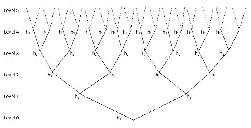
Let us consider some examples. Let m=2, k=2, then $G_{2}$ can be written as follows:

In this case, $G_{2}$-periodic function $h$ has the following form:

for $i_{k}\in\{1,2\}$ and $k\in V$.

In this paper, we consider the models where the spin takes values in the set $\Phi=\{1,2,\dots,q\}$ and is assigned to the vertices of the tree. A configuration $\sigma$ on V is then defined as a function $x\in V\rightarrow\sigma(x)\in\Phi$; the set of all configurations coincides with $\Omega=\Phi^{\Gamma^{k}}$. The Hamiltonian the $\lambda$-model has the following form

where the sum is taken over all pairs of nearest-neighbor vertices $\langle{x,y}\rangle$, $\sigma\in\Omega$. From a physical point of view the interactions between particles do not depend on their locations, therefore from now on we will assume that $\lambda$ is a symmetric function, i.e. $\lambda(u,v)=\lambda(v,u)$ for all $u,v\in\mathbb{R}$.

We note that $\lambda$-model of this type can be considered as generalization of the Potts model. The Potts model corresponds to the choice $\lambda(x,y)=-J\delta_{xy}$, where $x,y,J\in\mathbb{R}$.

In what follows, we restrict ourself to the case $k=2$ and $\Phi=\{1,2,3\}$, and for the sake of simplicity, we consider the following function:

where $\overline{a},\overline{b},\overline{c}\in\mathbb{R}$ for some given numbers.

In this section, we describe ground state of the $\lambda$-model on a Cayley tree. For a pair of configurations $\sigma$ and $\varphi$ coinciding almost everywhere, i.e., everywhere except finitely many points, we consider the relative Hamiltonian $H(\sigma,\varphi)$ determining the energy differences of the configurations $\sigma$ and $\varphi$:

For each $x\in V$, the set $\{x,S(x)\}$ is called a ball, and it is denoted by $b_{x}$. The set of all balls we denote by $M$.

We define the energy of the configuration $\sigma_{b}$ on b as follows

From (4), we got the following lemma.

A configuration $\varphi$ is called a ground state of the relative Hamiltonian $H$ if

for any $b\in M$

For any configuration $\sigma_{b}$, we have

where

We denote

Using (8), we obtain

Now, we want to find ground states for each considered cases. To do so, we introduce some notation. For each sequence $\{k_{0},k_{1},\dots,k_{n},\dots\},k_{n}\in\{1,2,3\}$, $n\in\mathbb{N}\cup\{0\}$, we define a configuration $\sigma$ on $\Omega$ by

This configuration is denoted by $\sigma_{[k_{n}]}$.

If the sequence $\{k_{0},k_{1},\dots,k_{n},\dots\}$ is $n$-periodic,(i.e. $k_{\ell+n}=k_{\ell},\forall n\in\mathbb{N}$), then instead of $\{k_{0},k_{1},\dots,k_{n},\dots\}$, we write $\{k_{0},k_{1},\dots,k_{n-1}\}$. Correspondingly, the associated configuration is denoted by $\sigma_{[k_{0},k_{1},\dots,k_{n-1}]}$

We define a finite-dimensional distribution of probability measure $\mu^{(n)}$ in a volume $V_{n}$ as

where $\beta=1/T$, $T>0$ is the temperature, and

is the normalizing factor. In (13), $\{h_{x}=(h_{1,x},\dots,h_{q,x})\in\mathbb{R},x\in V\}$ is the set of vectors, and

We say that sequence of a probability distribution $\{\mu^{(n)}\}$ is consistent if for all $n\geq 1$ and $\sigma_{n-1}\in\Phi^{V_{n-1}}$ one has

Here,$\sigma_{n-1}\vee\omega_{n}$ is the union of all configurations. In this case, we have a unique measure $\mu$ on $\Phi^{V}$ such that for all $n$ and $\sigma_{n}\in\Phi^{V_{n}}$, we have

Such a measure is called a splitting Gibbs measure corresponding to Hamiltonian (2) and to the vector-valued function $h_{x},x\in V$ (see [20] for more information about splitting measures).

The next statement describes the condition on $h_{x}$ ensuring that the sequence $\{\mu^{(n)}\}$ is consistent.

In this section, we are going to establish the existence of phase transition for the $\lambda$-model give by (3). As before, in what follows, we assume that $k=2$, $q=3$.

To establish a phase transition, we will find translation-invariant Gibbs measures. Here, by translation-invariant Gibbs measure we mean a splitting Gibbs measure which correspond to a solution $\mathbf{u}_{x}$ of the equation (19) which is translation-invariant, i.e. $\mathbf{u}_{x}=\mathbf{u}_{y}$ for all $x,y\in V$. This means $\mathbf{u}_{x}=\mathbf{u}$, where $\mathbf{u}=(u_{1},u_{2}),\ u_{1},u_{2}>0$. Due to Theorem 4.1, $u_{1}$ and $u_{2}$ must satisfy the following equation:

where $\theta_{1}=\exp\{\beta\overline{c}\},\ \theta_{2}=\exp\{\beta\overline{b}\},\ \theta_{3}=\exp\{\beta\overline{a}\}$ (here we have used (3)).

From (24) one can see that $u_{1}=1$ is invariant line of the equation. Therefore, the equation over this invariant line reduces to

Denoting

we rewrite (25) as follows:

Since $x>0,k\geq 1,a>0,$ and $b>0$;[18, Proposition 10.7] implies the following

References

• [1] R.J. Baxter, Exactly Solved Models in Statistical Mechanics, (Academic Press, London/New York, 1982).
• [2] R.L. Dobrushin, The description of a random field by means of conditional probabilities and conditions of its regularity,Theor. Probab. Appl. 13 (1968), 197–224.
• [3] S.N. Dorogovtsev, A.V. Goltsev, J.F.F.Mendes, Potts model on complex networks, Eur. Phys. J. B 38 (2004), 177-182.
• [4] N.N. Ganikhodjaev, On pure phases of the three-state ferromagnetic Potts model on the second-order Bethe lattice. Theor. Math. Phys. 85 (1990), 1125–1134.
• [5] N.N. Ganikhodjaev, F.M. Mukhamedov, J.F.F. Mendes, On the three state Potts model with competing interactions on the Bethe lattice, Jour. Stat. Mech. 2006, P08012, 29 p
• [6] N.N. Ganikhodjaev, U.A. Rozikov, On disordered phase in the ferromagnetic Potts model on the Bethe lattice. Osaka J. Math. 37 (2000), 373–383.
• [7] H.O. Georgii, Gibbs measures and phase transitions (Walter de Gruyter, Berlin, 1988).
• [8] S. Janson, E. Mossel, Robust reconstruction on trees is determined by the second eigenvalue. Ann. Probab. 32 (2004), 2630–2649.
• [9] M.C. Marques, Three-state Potts model with antiferromagnetic interactions: a MFRG approach, J.Phys. A: Math. Gen. 21(1988), 1061-1068.
• [10] F.M. Mukhamedov, On a factor associated with the unordered phase of λ\lambda-model on a Cayley tree. Rep. Math. Phys. 53 (2004), 1–18.
• [11] F.M.Mukhamedov and U.A.Rozikov, Extremality of the disordered phase of the nonhomogeneous Potts model on the Cayley tree. Theor. Math. Phys. 124 (2000), 1202–1210
• [12] M.P. Nightingale, M. Schick, Three-state square lattice Potts antiferromagnet, J.Phys. A: Math. Gen. 15 (1982), L39-L42.
• [13] F. Peruggi, Probability measures and Hamiltonian models on Bethe lattices. I. Properties and construction of MRT probability measures. J. Math. Phys. 25 (1984), 3303–3315.
• [14] F. Peruggi, Probability measures and Hamiltonian models on Bethe lattices. II. The solution of thermal and configurational problems. J. Math. Phys. 25 (1984), 3316–3323.
• [15] F. Peruggi, F. di Liberto, G. Monroy, Potts model on Bethe lattices. I. General results. J. Phys. A 16 (1983), 811–827.
• [16] F. Peruggi, F. di Liberto, G. Monroy, Phase diagrams of the qq-state Potts model on Bethe lattices. Physica A 141 (1987) 151–186.
• [17] R.B. Potts, Some generalized order-disorder transformations, Proc. Cambridge Philos. Soc. 48(1952), 106–109.
• [18] C. Preston, Gibbs states on countable sets (Cambridge University Press, London 1974).
• [19] U.A. Rozikov, Description of limit Gibbs measures for λ\lambda-models on the Bethe lattice, Siberan Math. Jour. 39(1998), 373–380.
• [20] Rozikov U.A. Gibbs Measures on Cayley Trees, World Scientific, Singapore, 2013.
• [21] A.N.Shiryaev,Probability (Nauka, Moscow, 1980).
• [22] P.N. Timonin, Inhomogeneity-induced second order phase transitions in the Potts models on hierarchical lattices. JETP 99 (2004), 1044–1053.
• [23] F.Y. Wu, The Potts model, Rev. Mod. Phys. 54 (1982), 235–268.