跳到论文正文
W Papers独立论文阅读器 arXiv:1610.06685 论文正文 计算阅读时间 · 0%
引用这篇论文根据当前论文元数据生成,正式投稿前建议核对。


License: arXiv.org perpetual non-exclusive license
arXiv:1610.06685v3 [math.NA] 10 Feb 2017

Error estimates with explicit constants for the Sinc approximation over infinite intervals Note: This work was partially supported by Grant-in-Aid for Young Scientists (B) Number JP24760060.

Journal: Elsevier
Tomoaki Okayama Address: Graduate School of Information Sciences, Hiroshima City University
3-4-1, Ozuka-higashi, Asaminami-ku, Hiroshima 731-3194, Japan
Email: okayama@hiroshima-cu.ac.jp
Abstract

The Sinc approximation is a function approximation formula that attains exponential convergence for rapidly decaying functions defined on the whole real axis. Even for other functions, the Sinc approximation works accurately when combined with a proper variable transformation. The convergence rate has been analyzed for typical cases including finite, semi-infinite, and infinite intervals. Recently, for verified numerical computations, a more explicit, “computable” error bound has been given in the case of a finite interval. In this paper, such explicit error bounds are derived for other cases.

Keywords: 
Sinc approximation , conformal map , double-exponential transformation , infinite interval , error bound
2010 MSC
65D05 , 65D15 , 65G99

1 Introduction

The “Sinc approximation” is a function approximation formula that can be expressed as

F⁡(x)≈∑k=−MNF⁡(k​h)​S​(k,h)​(x),x∈ℝ,F(x)\approx\sum_{k=-M}^{N}F(kh)S(k,h)(x),\quad x\in\mathbb{R}, (1.1)

where S​(k,h)​(x)S(k,h)(x) is the so-called Sinc function, defined by

S​(k,h)​(x)=sin⁡[π⁡(x/h−k)]π⁡(x/h−k),S(k,h)(x)=\frac{\sin[\piup(x/h-k)]}{\piup(x/h-k)},

and MM, NN, hh are selected according to the given positive integer nn. It is well known that the approximation formula (1.1) can converge exponentially when combined with an appropriate variable transformation. Furthermore, it has been shown that the approximation formula (1.1) is nearly optimal for functions in some Hardy spaces [1, 2]. Motivated by this fact, many researchers have studied applications of the Sinc approximation (see Stenger [3, 4], Lund–Bowers [5], Sugihara–Matsuo [6], and references therein).

As stated above, to attain exponential convergence, an appropriate variable transformation t=ψ⁡(x)t=\psi(x) is required. In this regard, depending on the target interval (a,b)(a,\,b) and the function ff, Stenger [3] considered the following four typical cases:

  1. 1.

    (a,b)=(−∞,∞)(a,\,b)=(-\infty,\,\infty) and |f⁡(t)||f(t)| decays algebraically as t→±∞t\to\pm\infty,

  2. 2.

    (a,b)=(0,∞)(a,\,b)=(0,\,\infty) and |f⁡(t)||f(t)| decays algebraically as t→∞t\to\infty,

  3. 3.

    (a,b)=(0,∞)(a,\,b)=(0,\,\infty) and |f⁡(t)||f(t)| decays (already) exponentially as t→∞t\to\infty,

  4. 4.

    The interval (a,b)(a,\,b) is finite.

In all four cases, Stenger gave the concrete transformations to be employed:

ψSE1​(x)=sinh⁡x,\displaystyle\psi_{\text{\tiny{\rm{SE$1$}}}}(x)=\sinh x, ψSE2​(x)=ex,\displaystyle\psi_{\text{\tiny{\rm{SE$2$}}}}(x)=\mathrm{e}^{x}, ψSE3​(x)=arcsinh⁡(ex),\displaystyle\psi_{\text{\tiny{\rm{SE$3$}}}}(x)=\arcsinh(\mathrm{e}^{x}), ψSE4​(x)=b−a2​tanh⁡(x2)+b+a2.\displaystyle\psi_{\text{\tiny{\rm{SE$4$}}}}(x)=\frac{b-a}{2}\tanh\left(\frac{x}{2}\right)+\frac{b+a}{2}.

These are called conformal maps in the literature. After applying the variable transformation t=ψSEi​(x)t=\psi_{\text{\tiny{\rm{SE$i$}}}}(x), we may set F⁡(x)=f⁡(ψSEi​(x))F(x)=f(\psi_{\text{\tiny{\rm{SE$i$}}}}(x)) and use the Sinc approximation (1.1). As a result, we have the following approximation for f⁡(t)f(t):

f⁡(t)≈∑k=−MNf⁡(ψSEi​(k​h))​S​(k,h)​(ψSEi−1​(t)),f(t)\approx\sum_{k=-M}^{N}f(\psi_{\text{\tiny{\rm{SE$i$}}}}(kh))S(k,h)(\psi_{\text{\tiny{\rm{SE$i$}}}}^{-1}(t)), (1.2)

which is referred to as the “SE-Sinc approximation” in this paper. Stenger [3] demonstrated the exponential convergence of the approximation (1.2) by giving error analyses in the following form:

supt∈(a,b)|f⁡(t)−∑k=−MNf⁡(ψSEi​(k​h))​S​(k,h)​(ψSEi−1​(t))|\displaystyle\sup_{t\in(a,\,b)}\left|f(t)-\sum_{k=-M}^{N}f(\psi_{\text{\tiny{\rm{SE$i$}}}}(kh))S(k,h)(\psi_{\text{\tiny{\rm{SE$i$}}}}^{-1}(t))\right| ≤C​n​e−π​d​μ​n,\displaystyle\leq C\sqrt{n}\rme^{-\sqrt{\piup d\mu n}}, (1.3)

where μ\mu and dd are positive parameters of the analytic properties of ff, and CC is a constant independent of nn.

In recent decades, several authors [6, 7, 8] have pointed out that the performance of the Sinc approximation can be improved by replacing the original variable transformations with the following ones:

ψDE1​(t)=ψSE1​(π2​sinh⁡t),\displaystyle\psi_{\text{\tiny{\rm{DE$1$}}}}(t)=\psi_{\text{\tiny{\rm{SE$1$}}}}\left(\frac{\piup}{2}\sinh t\right), ψDE2​(t)=ψSE2​(π2​sinh⁡t),\displaystyle\psi_{\text{\tiny{\rm{DE$2$}}}}(t)=\psi_{\text{\tiny{\rm{SE$2$}}}}\left(\frac{\piup}{2}\sinh t\right), ψDE3†​(t)=et−exp⁡(−t),\displaystyle\psi_{\text{\tiny{\rm{DE$3\dagger$}}}}(t)=\mathrm{e}^{t-\exp(-t)}, ψDE4​(t)=ψSE4​(π​sinh⁡t).\displaystyle\psi_{\text{\tiny{\rm{DE$4$}}}}(t)=\psi_{\text{\tiny{\rm{SE$4$}}}}\left(\piup\sinh t\right).

These are called the “Double-Exponential (DE) transformations,” and were originally introduced by Takahasi–Mori [9] for numerical integration. In addition, in case 3, another DE transformation

ψDE3​(t)=log⁡(1+e(π/2)​sinh⁡t)\psi_{\text{\tiny{\rm{DE$3$}}}}(t)=\log(1+\rme^{(\piup/2)\sinh t})

has been proposed [10] so that the inverse function can be explicitly written by using elementary functions (whereas ψDE3†​(t)\psi_{\text{\tiny{\rm{DE$3\dagger$}}}}(t) cannot). The combination of the DE transformation and (1.1) is called the “DE-Sinc approximation.” The error analyses for i=1i=1, 22, 33, 44 have been given [8] as

supt∈(a,b)|f⁡(t)−∑k=−nnf⁡(ψDEi​(k​h))​S​(k,h)​(ψDEi−1​(t))|\displaystyle\sup_{t\in(a,\,b)}\left|f(t)-\sum_{k=-n}^{n}f(\psi_{\text{\tiny{\rm{DE$i$}}}}(kh))S(k,h)(\psi_{\text{\tiny{\rm{DE$i$}}}}^{-1}(t))\right| ≤Ce−πdn/log(4dn/μ),\displaystyle\leq C\rme^{-\piup dn/\log(4dn/\mu)}, (1.4)
and for ψDE3†​(t)\psi_{\text{\tiny{\rm{DE$3\dagger$}}}}(t), also given [8] as
supt∈(0,∞)|f⁡(t)−∑k=−nnf⁡(ψDE3†​(k​h))​S​(k,h)​(ψDE3†−1​(t))|\displaystyle\sup_{t\in(0,\,\infty)}\left|f(t)-\sum_{k=-n}^{n}f(\psi_{\text{\tiny{\rm{DE$3\dagger$}}}}(kh))S(k,h)(\psi_{\text{\tiny{\rm{DE$3\dagger$}}}}^{-1}(t))\right| ≤Ce−πdn/log(πdn/μ).\displaystyle\leq C\rme^{-\piup dn/\log(\piup dn/\mu)}. (1.5)

The main objective of this study is to refine these error analyses into more useful forms. It should be emphasized that the error analyses (1.3), (1.4), and (1.5) are not just asymptotic (≃\simeq), but are strict inequalities (≤\leq). Hence, if the constants CC are given in a more explicit, computable form, we can use the term on the right-hand side as a rigorous error bound, which is quite useful for verified numerical computations. In fact, the explicit form of CC was revealed in case 4 (the interval is finite) [11]. This study reveals the explicit form of CC in cases 1–3 (the interval is not finite).

As a second objective, this paper improves the DE transformation in case 3. Instead of ψDE3​(t)\psi_{\text{\tiny{\rm{DE$3$}}}}(t) or ψDE3†​(t)\psi_{\text{\tiny{\rm{DE$3\dagger$}}}}(t),

ψDE3‡​(t)=log⁡(1+eπ​sinh⁡t)\psi_{\text{\tiny{\rm{DE$3\ddagger$}}}}(t)=\log(1+\rme^{\piup\sinh t})

is employed in this paper, which was originally proposed for numerical integration [12]. The error is also given as

supt∈(0,∞)|f(t)−∑k=−nnf(ψDE3‡(kh))S(k,h)(ψDE3‡−1(t))|≤Ce−πdn/log(2dn/μ),\sup_{t\in(0,\,\infty)}\left|f(t)-\sum_{k=-n}^{n}f(\psi_{\text{\tiny{\rm{DE$3\ddagger$}}}}(kh))S(k,h)(\psi_{\text{\tiny{\rm{DE$3\ddagger$}}}}^{-1}(t))\right|\leq C\rme^{-\piup dn/\log(2dn/\mu)}, (1.6)

with the explicit constant CC. The convergence rate of (1.6) is better than that of (1.4) or (1.5). Furthermore, in the same manner as for numerical integration [12], it can be shown that ψDE3‡\psi_{\text{\tiny{\rm{DE$3\ddagger$}}}} is the best possible variable transformation in case 3 (although this is not discussed in this paper).

The remainder of this paper is organized as follows. In Section 2, existing error analyses and new explicit error bounds (the main result) are stated. Numerical examples are presented in Section 3. Proofs of all the theorems stated in this paper are given in Section 4. Section 5 draws together our conclusions.

2 Existing error analyses and new error estimates with explicit constants

In this section, after reviewing existing results, new error bounds for the SE- and DE-Sinc approximations are stated. Let us first introduce some notation. Let 𝒟d\mathscr{D}_{d} be a strip domain defined by 𝒟d={ζ∈ℂ:|Imζ|<d}\mathscr{D}_{d}=\{\zeta\in\mathbb{C}:|\mathop{\mathrm{Im}}\nolimits\zeta|<d\} for d>0d>0. Furthermore, let 𝒟d−={ζ∈𝒟d:Reζ<0}\mathscr{D}_{d}^{-}=\{\zeta\in\mathscr{D}_{d}:\mathop{\mathrm{Re}}\nolimits\zeta<0\} and 𝒟d+={ζ∈𝒟d:Reζ≥0}\mathscr{D}_{d}^{+}=\{\zeta\in\mathscr{D}_{d}:\mathop{\mathrm{Re}}\nolimits\zeta\geq 0\}. In this section, dd is assumed to be a positive constant with d<π/2d<\piup/2. Let ψ⁡(𝒟d)\psi(\mathscr{D}_{d}) denote the image of 𝒟d\mathscr{D}_{d} given by the map ψ\psi, i.e., ψ⁡(𝒟d)={z=ψ⁡(ζ):ζ∈𝒟d}\psi(\mathscr{D}_{d})=\left\{z=\psi(\zeta):\zeta\in\mathscr{D}_{d}\right\}. Let I1=(−∞,∞)I_{1}=(-\infty,\,\infty), I2=I3=(0,∞)I_{2}=I_{3}=(0,\,\infty), and let us define the following three functions:

E1​(z,γ)\displaystyle E_{1}(z;\gamma) =1(1+z2)γ/2,\displaystyle=\frac{1}{(1+z^{2})^{\gamma/2}},
E2​(z,α,β)\displaystyle E_{2}(z;\alpha,\beta) =zα(1+z2)(α+β)/2,\displaystyle=\frac{z^{\alpha}}{(1+z^{2})^{(\alpha+\beta)/2}},
E3​(z,α,β)\displaystyle E_{3}(z;\alpha,\beta) =(z1+z)α​e−β​z.\displaystyle=\left(\frac{z}{1+z}\right)^{\alpha}\rme^{-\beta z}.

We write Ei​(z,γ,γ)E_{i}(z;\gamma,\gamma) as Ei​(z,γ)E_{i}(z;\gamma) for short.

2.1 Existing error analyses and new error estimates for the SE-Sinc approximation

Existing error analyses for the Sinc approximation combined with ψSE1\psi_{\text{\tiny{\rm{SE$1$}}}}, ψSE2\psi_{\text{\tiny{\rm{SE$2$}}}}, and ψSE3\psi_{\text{\tiny{\rm{SE$3$}}}} are written in the following form (Theorems 2.1 and 2.2).

Theorem 2.1 (Stenger [3, Theorem 4.2.5])

Assume that ff is analytic in ψSE1​(𝒟d)\psi_{\text{\tiny{\rm{SE$1$}}}}(\mathscr{D}_{d}), and that there exist positive constants KK, α\alpha, and β\beta such that

|f⁡(z)|\displaystyle|f(z)| ≤K​|E1​(z,α)|\displaystyle\leq K|E_{1}(z;\alpha)| (2.1)
for all z∈ψSE1​(𝒟d−)z\in\psi_{\text{\tiny{\rm{SE$1$}}}}(\mathscr{D}_{d}^{-}), and
|f⁡(z)|\displaystyle|f(z)| ≤K​|E1​(z,β)|\displaystyle\leq K|E_{1}(z;\beta)| (2.2)

for all z∈ψSE1​(𝒟d+)z\in\psi_{\text{\tiny{\rm{SE$1$}}}}(\mathscr{D}_{d}^{+}). Let μ=min⁡{α,β}\mu=\min\{\alpha,\,\beta\}, let hh be defined as

h=π​dμ​n,h=\sqrt{\frac{\piup d}{\mu n}}, (2.3)

and let MM and NN be defined as

{M=n,N=⌈α​n/β⌉(if​μ=α),N=n,M=⌈β​n/α⌉(if​μ=β).\begin{cases}M=n,\quad N=\lceil\alpha n/\beta\rceil&\,\,\,(\text{if}\,\,\,\mu=\alpha),\\ N=n,\quad M=\lceil\beta n/\alpha\rceil&\,\,\,(\text{if}\,\,\,\mu=\beta).\end{cases} (2.4)

Then, there exists a constant C1C_{1}, independent of nn, such that

supt∈I1|f⁡(t)−∑k=−MNf⁡(ψSE1​(k​h))​S​(k,h)​(ψSE1−1​(t))|≤C1​n​e−π​d​μ​n.\sup_{t\in I_{1}}\left|f(t)-\sum_{k=-M}^{N}f(\psi_{\text{\tiny{\rm{SE$1$}}}}(kh))S(k,h)(\psi_{\text{\tiny{\rm{SE$1$}}}}^{-1}(t))\right|\leq C_{1}\sqrt{n}\rme^{-\sqrt{\piup d\mu n}}. (2.5)
Theorem 2.2 (Stenger [3, Theorem 4.2.5])

The following is true for i=2i=2, 33. Assume that ff is analytic in ψSEi​(𝒟d)\psi_{\text{\tiny{\rm{SE$i$}}}}(\mathscr{D}_{d}), and that there exist positive constants KK, α\alpha, and β\beta such that

|f⁡(z)|≤K​|Ei​(z,α,β)||f(z)|\leq K|E_{i}(z;\alpha,\beta)| (2.6)

for all z∈ψSEi​(𝒟d)z\in\psi_{\text{\tiny{\rm{SE$i$}}}}(\mathscr{D}_{d}). Let μ=min⁡{α,β}\mu=\min\{\alpha,\,\beta\}, let hh be defined as in (2.3), and let MM and NN be defined as in (2.4). Then, there exists a constant CiC_{i}, independent of nn, such that

supt∈Ii|f⁡(t)−∑k=−MNf⁡(ψSEi​(k​h))​S​(k,h)​(ψSEi−1​(t))|≤Ci​n​e−π​d​μ​n.\sup_{t\in I_{i}}\left|f(t)-\sum_{k=-M}^{N}f(\psi_{\text{\tiny{\rm{SE$i$}}}}(kh))S(k,h)(\psi_{\text{\tiny{\rm{SE$i$}}}}^{-1}(t))\right|\leq C_{i}\sqrt{n}\rme^{-\sqrt{\piup d\mu n}}. (2.7)

This paper explicitly estimates the constant CiC_{i} in (2.5) and (2.7) as follows.

Theorem 2.3

Let the assumptions in Theorem 2.1 be fulfilled. Furthermore, let ν=max⁡{α,β}\nu=\max\{\alpha,\,\beta\}. Then, inequality (2.5) holds with

C1=2ν+1​Kπ​d​μ​{2π​d​μ​(1−e−2​π​d​μ)​{cos⁡d}ν+1}.C_{1}=\frac{2^{\nu+1}K}{\sqrt{\piup d\mu}}\left\{\frac{2}{\sqrt{\piup d\mu}(1-\rme^{-2\sqrt{\piup d\mu}})\{\cos d\}^{\nu}}+1\right\}.
Theorem 2.4

Let the assumptions in Theorem 2.2 be fulfilled. Then, inequality (2.7) holds with

C2\displaystyle C_{2} =2​Kπ​d​μ​{2π​d​μ​(1−e−2​π​d​μ)​{cos⁡d}(α+β)/2+1},\displaystyle=\frac{2K}{\sqrt{\piup d\mu}}\left\{\frac{2}{\sqrt{\piup d\mu}(1-\rme^{-2\sqrt{\piup d\mu}})\{\cos d\}^{(\alpha+\beta)/2}}+1\right\},
C3\displaystyle C_{3} =2​Kπ​d​μ​{21+(α+β)/2π​d​μ​(1−e−2​π​d​μ)​{cos⁡(d/2)}α+β+1}.\displaystyle=\frac{2K}{\sqrt{\piup d\mu}}\left\{\frac{2^{1+(\alpha+\beta)/2}}{\sqrt{\piup d\mu}(1-\rme^{-2\sqrt{\piup d\mu}})\{\cos(d/2)\}^{\alpha+\beta}}+1\right\}.

2.2 Existing error analyses and new error estimates for the DE-Sinc approximation

Existing error analyses for the Sinc approximation with ψDE1\psi_{\text{\tiny{\rm{DE$1$}}}}, ψDE2\psi_{\text{\tiny{\rm{DE$2$}}}}, ψDE3\psi_{\text{\tiny{\rm{DE$3$}}}}, and ψDE3†\psi_{\text{\tiny{\rm{DE$3\dagger$}}}} are written in the following form (Theorems 2.5 and 2.6).

Theorem 2.5 (Tanaka et al. [8, Theorems 3.2, 3.3, 3.5])

The following is true for i=1i=1, 22, 33. Assume that ff is analytic in ψDEi​(𝒟d)\psi_{\text{\tiny{\rm{DE$i$}}}}(\mathscr{D}_{d}), and that there exist positive constants KK and μ\mu such that |f⁡(z)|≤K​|Ei​(z,μ)||f(z)|\leq K|E_{i}(z;\mu)| for all z∈ψDEi​(𝒟d)z\in\psi_{\text{\tiny{\rm{DE$i$}}}}(\mathscr{D}_{d}). Then, there exists a constant CiC_{i}, independent of nn, such that

supt∈Ii|f(t)−∑k=−nnf(ψDEi(kh))S(k,h)(ψDEi−1(t))|≤Cie−πdn/log(4dn/μ),\sup_{t\in I_{i}}\left|f(t)-\sum_{k=-n}^{n}f(\psi_{\text{\tiny{\rm{DE$i$}}}}(kh))S(k,h)(\psi_{\text{\tiny{\rm{DE$i$}}}}^{-1}(t))\right|\leq C_{i}\rme^{-\piup dn/\log(4dn/\mu)},

where

h=log⁡(4​d​n/μ)n.h=\frac{\log(4dn/\mu)}{n}. (2.8)
Remark 1

Strictly speaking, in case 3, the range of dd is not 0<d<π/20<d<\piup/2 (assumed at the beginning of this section), but 0<d<Imζ0≃1.40450<d<\mathop{\mathrm{Im}}\nolimits\zeta_{0}\simeq 1.4045, where ζ0=arcsinh⁡(2​i+2π​log⁡(1−1e))\zeta_{0}=\arcsinh(2\imnum+\frac{2}{\piup}\log(1-\frac{1}{\rme})). This is because the denominator of E3​(z,α,β)E_{3}(z;\alpha,\beta) is zero at z=ψDE3​(ζ0)z=\psi_{\text{\tiny{\rm{DE$3$}}}}(\zeta_{0}). To address this issue, this paper employs the function zμ​e−μ​zz^{\mu}\rme^{-\mu z} in Theorem 2.9 instead of E3​(z,μ)E_{3}(z;\mu).

Theorem 2.6 (Tanaka et al. [8, Theorem 3.4])

Assume that ff is analytic in ψDE3†​(𝒟d)\psi_{\text{\tiny{\rm{DE$3\dagger$}}}}(\mathscr{D}_{d}), and that there exist positive constants KK and μ\mu such that |f⁡(z)|≤K​|E3​(z,μ)||f(z)|\leq K|E_{3}(z;\mu)| for all z∈ψDE3†​(𝒟d)z\in\psi_{\text{\tiny{\rm{DE$3\dagger$}}}}(\mathscr{D}_{d}). Let hh be defined as h=log⁡(π​d​n/μ)/nh=\log(\piup dn/\mu)/n. Then, there exists a constant CC, independent of nn, such that (1.5) holds.

As for case 1 (Theorem 2.5 with i=1i=1) and case 2 (Theorem 2.5 with i=2i=2), this paper not only explicitly estimates the constants CiC_{i}, but also generalizes the approximation formula from ∑k=−nn\sum_{k=-n}^{n} to ∑k=−MN\sum_{k=-M}^{N} as stated below.

Theorem 2.7

Assume that ff is analytic in ψDE1​(𝒟d)\psi_{\text{\tiny{\rm{DE$1$}}}}(\mathscr{D}_{d}), and that there exist positive constants KK, α\alpha, and β\beta such that (2.1) holds for all z∈ψDE1​(𝒟d−)z\in\psi_{\text{\tiny{\rm{DE$1$}}}}(\mathscr{D}_{d}^{-}), and (2.2) holds for all z∈ψDE1​(𝒟d+)z\in\psi_{\text{\tiny{\rm{DE$1$}}}}(\mathscr{D}_{d}^{+}). Let μ=min⁡{α,β}\mu=\min\{\alpha,\,\beta\}, let ν=max⁡{α,β}\nu=\max\{\alpha,\,\beta\}, let hh be defined as in (2.8), and let MM and NN be defined as

{M=n,N=n−⌊log⁡(β/α)/h⌋(if​μ=α),N=n,M=n−⌊log⁡(α/β)/h⌋(if​μ=β).\begin{cases}M=n,\quad N=n-\lfloor\log(\beta/\alpha)/h\rfloor&\,\,\,(\text{if}\,\,\,\mu=\alpha),\\ N=n,\quad M=n-\lfloor\log(\alpha/\beta)/h\rfloor&\,\,\,(\text{if}\,\,\,\mu=\beta).\end{cases} (2.9)

Furthermore, let nn be taken sufficiently large so that n≥(ν​e)/(4​d)n\geq(\nu\rme)/(4d) holds. Then, it holds that

supt∈I1|f(t)−∑k=−MNf(ψDE1(kh))S(k,h)(ψDE1−1(t))|≤C1e−πdn/log(4dn/μ),\sup_{t\in I_{1}}\left|f(t)-\sum_{k=-M}^{N}f(\psi_{\text{\tiny{\rm{DE$1$}}}}(kh))S(k,h)(\psi_{\text{\tiny{\rm{DE$1$}}}}^{-1}(t))\right|\leq C_{1}\rme^{-\piup dn/\log(4dn/\mu)},

where C1C_{1} is a constant independent of nn, expressed as

C1=2ν+1​Kπ​d​μ​{4π(1−e−πμe/2){cos(π2sind)}νcosd+μ​eπ​ν/4}.C_{1}=\frac{2^{\nu+1}K}{\piup d\mu}\left\{\frac{4}{\piup(1-\rme^{-\piup\mu\rme/2})\{\cos(\frac{\piup}{2}\sin d)\}^{\nu}\cos d}+\mu\rme^{\piup\nu/4}\right\}.
Theorem 2.8

Assume that ff is analytic in ψDE2​(𝒟d)\psi_{\text{\tiny{\rm{DE$2$}}}}(\mathscr{D}_{d}), and that there exist positive constants KK, α\alpha, and β\beta such that (2.6) holds with i=2i=2 for all z∈ψDE2​(𝒟d)z\in\psi_{\text{\tiny{\rm{DE$2$}}}}(\mathscr{D}_{d}). Let μ=min⁡{α,β}\mu=\min\{\alpha,\,\beta\}, let ν=max⁡{α,β}\nu=\max\{\alpha,\,\beta\}, let hh be defined as in (2.8), and let MM and NN be defined as in (2.9). Furthermore, let nn be taken sufficiently large so that n≥(ν​e)/(4​d)n\geq(\nu\rme)/(4d) holds. Then, it holds that

supt∈I2|f(t)−∑k=−MNf(ψDE2(kh))S(k,h)(ψDE2−1(t))|≤C2e−πdn/log(4dn/μ),\sup_{t\in I_{2}}\left|f(t)-\sum_{k=-M}^{N}f(\psi_{\text{\tiny{\rm{DE$2$}}}}(kh))S(k,h)(\psi_{\text{\tiny{\rm{DE$2$}}}}^{-1}(t))\right|\leq C_{2}\rme^{-\piup dn/\log(4dn/\mu)},

where C2C_{2} is a constant independent of nn, expressed as

C2=2​Kπ​d​μ​{4π(1−e−πμe/2){cos(π2sind)}(α+β)/2cosd+μ​eπ​ν/4}.C_{2}=\frac{2K}{\piup d\mu}\left\{\frac{4}{\piup(1-\rme^{-\piup\mu\rme/2})\{\cos(\frac{\piup}{2}\sin d)\}^{(\alpha+\beta)/2}\cos d}+\mu\rme^{\piup\nu/4}\right\}.

As for case 3 (Theorem 2.5 with i=3i=3 and Theorem 2.6), this paper employs the improved variable transformation ψDE3‡\psi_{\text{\tiny{\rm{DE$3\ddagger$}}}} as described in the introduction, and gives the error estimates in a similar form to Theorems 2.7 and 2.8.

Theorem 2.9

Assume that ff is analytic in ψDE3‡​(𝒟d)\psi_{\text{\tiny{\rm{DE$3\ddagger$}}}}(\mathscr{D}_{d}), and that there exist positive constants KK and μ\mu (μ≤1\mu\leq 1) such that |f⁡(z)|≤K​|zμ​e−μ​z||f(z)|\leq K|z^{\mu}\rme^{-\mu z}| holds for all z∈ψDE3‡​(𝒟d)z\in\psi_{\text{\tiny{\rm{DE$3\ddagger$}}}}(\mathscr{D}_{d}). Let hh be defined as

h=log⁡(2​d​n/μ)n.h=\frac{\log(2dn/\mu)}{n}. (2.10)

Furthermore, let nn be taken sufficiently large so that n≥(μ​e)/(2​d)n\geq(\mu\rme)/(2d) holds. Then, inequality (1.6) holds with

C=Kπ1−μ​d​μ​{4π⁡(1−e−π​μ​e)​{cos⁡(π2​sin⁡d)}2​μ​{cos⁡d}μ+1+μ​21−μ​eμ⁡(π+2)/2}.C=\frac{K}{\piup^{1-\mu}d\mu}\left\{\frac{4}{\piup(1-\rme^{-\piup\mu\rme})\{\cos(\frac{\piup}{2}\sin d)\}^{2\mu}\{\cos d\}^{\mu+1}}+\mu 2^{1-\mu}\rme^{\mu(\piup+2)/2}\right\}.
Remark 2

In Theorem 2.9, the sum of the approximation formula is not ∑k=−MN\sum_{k=-M}^{N}, but ∑k=−nn\sum_{k=-n}^{n}. This is because the inequality bounding the function ff is not |f⁡(z)|≤K~​|zα​e−β​z||f(z)|\leq\tilde{K}|z^{\alpha}\rme^{-\beta z}|, but |f⁡(z)|≤K​|zμ​e−μ​z||f(z)|\leq K|z^{\mu}\rme^{-\mu z}|, which assumes α=β\alpha=\beta. This assumption, however, is made without loss of generality, because by setting z=(α/β)​wz=(\alpha/\beta)w and g⁡(w)=f⁡((α/β)​w)g(w)=f((\alpha/\beta)w) in the former inequality, we obtain |g⁡(w)|≤K~​(α/β)α​|wα​e−α​w||g(w)|\leq\tilde{K}(\alpha/\beta)^{\alpha}|w^{\alpha}\rme^{-\alpha w}|.

Remark 3

Theorems 2.1–2.4 assume that ff is analytic in a simply connected domain. In contrast, Theorems 2.5–2.9 assume that ff is analytic in an infinitely sheeted Riemann surface. These two assumptions are different; see Tanaka et al. [8, Figures 1–9] for details.

3 Numerical Examples

In this section, some numerical results are presented. All computation programs were written in C with double-precision floating-point arithmetic. The programs and computation results are available at https://github.com/okayamat/sinc-errorbound-infinite.

First, let us consider the following three examples.

Example 1 (Case 1: function decays algebraically as t→±∞t\to\pm\infty)

Consider the function

f1​(t)=11+t2​1+tanh2⁡(arcsinh⁡t),f_{1}(t)=\frac{1}{1+t^{2}}\sqrt{1+\tanh^{2}(\arcsinh t)},

which satisfies the assumptions in Theorem 2.3 with α=β=2\alpha=\beta=2, d=π/4d=\piup/4, and K=3/2K=3/2, and also those in Theorem 2.7 with α=β=2\alpha=\beta=2, d=π/6d=\piup/6, and K=3/2K=3/2.

Example 2 (Case 2: function decays algebraically as t→∞t\to\infty)

Consider the function

f2​(t)=t1+t2​1+tanh2⁡(log⁡t),f_{2}(t)=\frac{\sqrt{t}}{1+t^{2}}\sqrt{1+\tanh^{2}(\log t)},

which satisfies the assumptions in Theorem 2.4 (i=2i=2) with α=1/2\alpha=1/2, β=3/2\beta=3/2, d=π/4d=\piup/4, and K=3/2K=3/2, and also those in Theorem 2.8 with α=1/2\alpha=1/2, β=3/2\beta=3/2, d=π/6d=\piup/6, and K=3/2K=3/2.

Example 3 (Case 3: function decays exponentially as t→∞t\to\infty)

Consider the function

f3​(t)=tπ/4​e−t,f_{3}(t)=t^{\piup/4}\rme^{-t},

which satisfies the assumptions in Theorem 2.4 (i=3i=3) with α=π/4\alpha=\piup/4, β=3/4\beta=3/4, d=3.14/2d=3.14/2, and K=(1+(π/2)2)π/8K=(1+(\piup/2)^{2})^{\piup/8}, and also those in Theorem 2.5 (i=3i=3) with μ=π/4\mu=\piup/4, d=1.40d=1.40, and some constant K>0K>0 (note that no explicit error bound is given). In addition, if we set g⁡(u)=f3​((π/4)​u)g(u)=f_{3}((\piup/4)u), gg satisfies the assumptions in Theorem 2.9 with μ=π/4\mu=\piup/4, d=3/2d=3/2, and K=(π/4)π/4K=(\piup/4)^{\piup/4}.

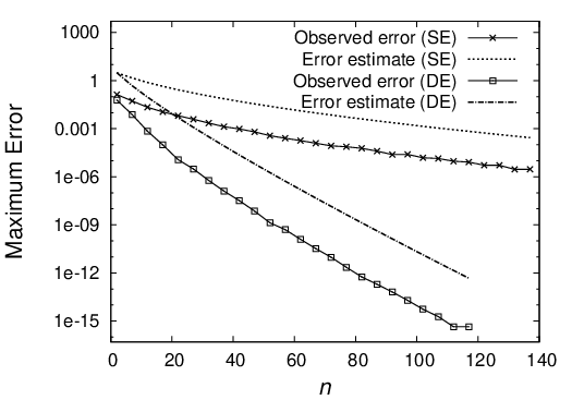
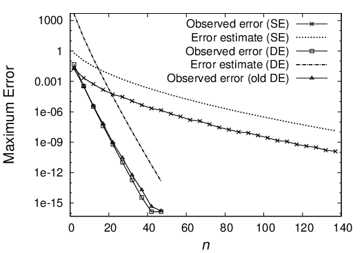
Numerical results are shown in Figures 4–4. In Figure 4, “Maximum Error” denotes the maximum value of the absolute error investigated at the following 403 points: t=0t=0, ±2−50\pm 2^{-50}, ±2−49.5,…\pm 2^{-49.5},\,\ldots, ±2−0.5\pm 2^{-0.5}, ±20\pm 2^{0}, ±20.5,…\pm 2^{0.5},\,\ldots, ±250\pm 2^{50}. Similarly, Figures 4 and 4 present the maximum errors at 201 points (positive points of those stated above). In each graph, we can see that the error estimate by the presented theorem (dotted line) clearly bounds the actual error (solid line). Furthermore, in Figure 4, we can confirm that the proposed DE-Sinc approximation using ψDE3‡\psi_{\text{\tiny{\rm{DE$3\ddagger$}}}} converges faster than the old DE-Sinc approximation using ψDE3\psi_{\text{\tiny{\rm{DE$3$}}}} (“old DE” in the graph). Another DE transformation ψDE3†\psi_{\text{\tiny{\rm{DE$3\dagger$}}}} is not employed, because ψDE3†−1\psi_{\text{\tiny{\rm{DE$3\dagger$}}}}^{-1} is not easily computed.

Next, let us consider the following example, which is an unfavorable case for the DE-Sinc approximation.

Example 4 (Case 1: function decays algebraically as t→±∞t\to\pm\infty)

Consider the function

f4​(t)=11+t2​cos⁡(3​arcsinh⁡t)+cosh⁡(π),f_{4}(t)=\frac{1}{1+t^{2}}\sqrt{\cos(3\arcsinh t)+\cosh(\piup)},

which satisfies the assumptions in Theorem 2.3 with α=β=2\alpha=\beta=2, d=π/3d=\piup/3, and K=2​cosh⁡(π)K=2\cosh(\piup), whereas it does not satisfy the assumptions in Theorem 2.7 as we cannot find any d>0d>0 such that f4f_{4} is analytic in ψDE1​(𝒟d)\psi_{\text{\tiny{\rm{DE$1$}}}}(\mathscr{D}_{d}) (we find α=β=2\alpha=\beta=2, though).

According to Okayama et al. [13], even in this case, the DE-Sinc approximation works almost as well as the SE-Sinc approximation by choosing d=arcsin⁡(dSE/π)d=\arcsin(d_{\text{\tiny{\rm{SE$$}}}}/\piup), where dSEd_{\text{\tiny{\rm{SE$$}}}} denotes dd in the SE-Sinc approximation. Actually, as shown in Figure 4, the DE-Sinc approximation converges at a similar rate to that of the SE-Sinc approximation. However, note that the error in the DE-Sinc approximation cannot be estimated by Theorem 2.7, whereas Theorem 2.3 works well.

Refer to caption
Figure 1: Approximation errors of f1f_{1} and their estimates.

Refer to caption
Figure 2: Approximation errors of f2f_{2} and their estimates.
Refer to caption
Figure 3: Approximation errors of f3f_{3} and their estimates.

Refer to caption
Figure 4: Approximation errors of f4f_{4} and their estimates.

4 Proofs

4.1 In the case of the SE-Sinc approximation

First, the error of the SE-Sinc approximation (1.2) is estimated. Let us look at a sketch of the proof. Let F⁡(x)=f⁡(ψSEi​(x))F(x)=f(\psi_{\text{\tiny{\rm{SE$i$}}}}(x)) (recall that we employ t=ψSEi​(x)t=\psi_{\text{\tiny{\rm{SE$i$}}}}(x) for the variable transformation), and evaluate the following term:

|f⁡(t)−∑k=−MNf⁡(ψSEi​(k​h))​S​(k,h)​(ψSEi−1​(t))|=|F⁡(x)−∑k=−MNF⁡(k​h)​S​(k,h)​(x)|,\displaystyle\left|f(t)-\sum_{k=-M}^{N}f(\psi_{\text{\tiny{\rm{SE$i$}}}}(kh))S(k,h)(\psi_{\text{\tiny{\rm{SE$i$}}}}^{-1}(t))\right|=\left|F(x)-\sum_{k=-M}^{N}F(kh)S(k,h)(x)\right|,

which is the error of the Sinc approximation (1.1). For the estimation, the following function space plays an important role.

Definition 4.1

Let L,R,α,β,γL,\,R,\,\alpha,\,\beta,\,\gamma be positive constants, and let dd be a constant with 0<d<π/γ0<d<\piup/\gamma. Then, 𝐋L,R,α,β,γSE​(𝒟d)\mathbf{L}_{L,R,\alpha,\beta,\gamma}^{\text{\scriptsize{\rm{SE}}}}(\mathscr{D}_{d}) denotes a family of functions FF that are analytic in 𝒟d\mathscr{D}_{d}, and for all ζ∈𝒟d\zeta\in\mathscr{D}_{d} and x∈ℝx\in\mathbb{R}, satisfy

|F⁡(ζ)|\displaystyle|F(\zeta)| ≤L|1+e−γ​ζ|α/γ​|1+eγ​ζ|β/γ,\displaystyle\leq\frac{L}{|1+\rme^{-\gamma\zeta}|^{\alpha/\gamma}|1+\rme^{\gamma\zeta}|^{\beta/\gamma}}, (4.1)
|F⁡(x)|\displaystyle|F(x)| ≤R(1+e−γ​x)α/γ​(1+eγ​x)β/γ.\displaystyle\leq\frac{R}{(1+\rme^{-\gamma x})^{\alpha/\gamma}(1+\rme^{\gamma x})^{\beta/\gamma}}. (4.2)

If F∈𝐋L,R,α,β,γSE​(𝒟d)F\in\mathbf{L}_{L,R,\alpha,\beta,\gamma}^{\text{\scriptsize{\rm{SE}}}}(\mathscr{D}_{d}), the error of the Sinc approximation is estimated as below. The proof is omitted here because it is quite similar to that of the existing theorem for case 4 [11, Theorem 2.4].

Theorem 4.10

Let F∈𝐋L,R,α,β,γSE​(𝒟d)F\in\mathbf{L}_{L,R,\alpha,\beta,\gamma}^{\text{\scriptsize{\rm{SE}}}}(\mathscr{D}_{d}), let μ=min⁡{α,β}\mu=\min\{\alpha,\,\beta\}, let hh be defined as in (2.3), and let MM and NN be defined as in (2.4). Then, setting ϵnSE=n​e−π​d​μ​n\epsilon_{n}^{\text{\scriptsize{\rm{SE}}}}=\sqrt{n}\rme^{-\sqrt{\piup d\mu n}}, we have

supx∈ℝ|F⁡(x)−∑k=−MNF⁡(k​h)​S​(k,h)​(x)|≤2π​d​μ​[2​Lπ​d​μ​(1−e−2​π​d​μ)​{cos⁡(γ​d/2)}(α+β)/γ+R]​ϵnSE.\sup_{x\in\mathbb{R}}\left|F(x)-\sum_{k=-M}^{N}F(kh)S(k,h)(x)\right|\leq\frac{2}{\sqrt{\piup d\mu}}\left[\frac{2L}{\sqrt{\piup d\mu}(1-\rme^{-2\sqrt{\piup d\mu}})\{\cos(\gamma d/2)\}^{(\alpha+\beta)/\gamma}}+R\right]\epsilon_{n}^{\text{\scriptsize{\rm{SE}}}}.

In view of Theorem 4.10, the proof is completed by checking F∈𝐋L,R,α,β,γSE​(𝒟d)F\in\mathbf{L}_{L,R,\alpha,\beta,\gamma}^{\text{\scriptsize{\rm{SE}}}}(\mathscr{D}_{d}) for cases 1, 2, and 3. Let us examine each case individually.

4.1.1 Proof in case 1 (Theorem 2.3)

The claim of Theorem 2.3 follows from the next lemma.

Lemma 4.11

Let the assumptions in Theorem 2.3 be fulfilled. Then, the function F⁡(ζ)=f⁡(ψSE1​(ζ))F(\zeta)=f(\psi_{\text{\tiny{\rm{SE$1$}}}}(\zeta)) belongs to 𝐋L,R,α,β,γSE​(𝒟d)\mathbf{L}_{L,R,\alpha,\beta,\gamma}^{\text{\scriptsize{\rm{SE}}}}(\mathscr{D}_{d}) with L=2ν​K/{cos⁡d}(ν−μ)/2L=2^{\nu}K/\{\cos d\}^{(\nu-\mu)/2}, R=2ν​KR=2^{\nu}K, and γ=2\gamma=2.

The proof is straightforward by the next result, because |F⁡(ζ)|≤K​|E1​(ψSE1​(ζ),α)||F(\zeta)|\leq K|E_{1}(\psi_{\text{\tiny{\rm{SE$1$}}}}(\zeta);\alpha)| and |F⁡(ζ)|≤K​|E2​(ψSE1​(ζ),β)||F(\zeta)|\leq K|E_{2}(\psi_{\text{\tiny{\rm{SE$1$}}}}(\zeta);\beta)| coincide with the inequalities in the following lemma.

Lemma 4.12 (Okayama [12, in the proof of Lemma 5.1])

Assume that FF is analytic in 𝒟d\mathscr{D}_{d} with 0<d<π/20<d<\piup/2, and that there exist positive constants KK, α\alpha, β\beta such that

|F⁡(ζ)|\displaystyle|F(\zeta)| ≤K|1+e−2​ζ|α/2​|1+e2​ζ|α/2\displaystyle\leq\frac{K}{|1+\rme^{-2\zeta}|^{\alpha/2}|1+\rme^{2\zeta}|^{\alpha/2}}
holds for all ζ∈𝒟d−\zeta\in\mathscr{D}_{d}^{-}, and
|F⁡(ζ)|\displaystyle|F(\zeta)| ≤K|1+e−2​ζ|β/2​|1+e2​ζ|β/2\displaystyle\leq\frac{K}{|1+\rme^{-2\zeta}|^{\beta/2}|1+\rme^{2\zeta}|^{\beta/2}}

holds for all ζ∈𝒟d+\zeta\in\mathscr{D}_{d}^{+}. Then, F∈𝐋L,R,α,β,γSE​(𝒟d)F\in\mathbf{L}_{L,R,\alpha,\beta,\gamma}^{\text{\scriptsize{\rm{SE}}}}(\mathscr{D}_{d}) with L=2ν​K/{cos⁡d}(ν−μ)/2L=2^{\nu}K/\{\cos d\}^{(\nu-\mu)/2}, R=2ν​KR=2^{\nu}K, and γ=2\gamma=2, where μ=min⁡{α,β}\mu=\min\{\alpha,\,\beta\} and ν=max⁡{α,β}\nu=\max\{\alpha,\,\beta\}.

4.1.2 Proof in case 2 (Theorem 2.4 with i=2i=2)

The claim of Theorem 2.4 with i=2i=2 follows from the next lemma.

Lemma 4.13

Let the assumptions in Theorem 2.4 be fulfilled with i=2i=2. Then, the function F⁡(ζ)=f⁡(ψSE2​(ζ))F(\zeta)=f(\psi_{\text{\tiny{\rm{SE$2$}}}}(\zeta)) belongs to 𝐋L,R,α,β,γSE​(𝒟d)\mathbf{L}_{L,R,\alpha,\beta,\gamma}^{\text{\scriptsize{\rm{SE}}}}(\mathscr{D}_{d}) with L=KL=K, R=KR=K, and γ=2\gamma=2.

Proof 1

From inequality (2.6) with i=2i=2, (4.1) and (4.2) immediately hold with L=R=KL=R=K and γ=2\gamma=2.

4.1.3 Proof in case 3 (Theorem 2.4 with i=3i=3)

The claim of Theorem 2.4 follows from the next lemma.

Lemma 4.14

Let the assumptions in Theorem 2.4 be fulfilled with i=3i=3. Then, the function F⁡(ζ)=f⁡(ψSE3​(ζ))F(\zeta)=f(\psi_{\text{\tiny{\rm{SE$3$}}}}(\zeta)) belongs to 𝐋L,R,α,β,γSE​(𝒟d)\mathbf{L}_{L,R,\alpha,\beta,\gamma}^{\text{\scriptsize{\rm{SE}}}}(\mathscr{D}_{d}) with L=2(α+β)/2​KL=2^{(\alpha+\beta)/2}K, R=KR=K, and γ=1\gamma=1.

For the proof, let us prepare some useful inequalities (Lemmas 4.15 and 4.16).

Lemma 4.15 (Okayama [12, Lemma 5.4])

For all ζ∈𝒟π/2¯\zeta\in\overline{\mathscr{D}_{\piup/2}} and x∈ℝx\in\mathbb{R}, we have

|arcsinh⁡(eζ)1+arcsinh⁡(eζ)|\displaystyle\left|\frac{\arcsinh(\rme^{\zeta})}{1+\arcsinh(\rme^{\zeta})}\right| ≤2​|eζ1+eζ|,\displaystyle\leq\sqrt{2}\left|\frac{\rme^{\zeta}}{1+\rme^{\zeta}}\right|,
arcsinh⁡(ex)1+arcsinh⁡(ex)\displaystyle\frac{\arcsinh(\rme^{x})}{1+\arcsinh(\rme^{x})} ≤ex1+ex.\displaystyle\leq\frac{\rme^{x}}{1+\rme^{x}}.
Lemma 4.16 (Okayama [12, Lemma 5.5])

For all ζ∈𝒟π/2¯\zeta\in\overline{\mathscr{D}_{\piup/2}} and x∈ℝx\in\mathbb{R}, we have

1|eζ+1+e2​ζ|\displaystyle\frac{1}{|\rme^{\zeta}+\sqrt{1+\rme^{2\zeta}}|} ≤2|1+eζ|,\displaystyle\leq\frac{\sqrt{2}}{|1+\rme^{\zeta}|},
1ex+1+e2​x\displaystyle\frac{1}{\rme^{x}+\sqrt{1+\rme^{2x}}} ≤11+ex.\displaystyle\leq\frac{1}{1+\rme^{x}}.

By using the lemmas above, Lemma 4.14 can be proved as follows.

Proof 2

From inequality (2.6) with i=3i=3, it follows that

|F⁡(ζ)|≤K​|arcsinh⁡(eζ)1+arcsinh⁡(eζ)|α​|1eζ+1+e2​ζ|β.\displaystyle|F(\zeta)|\leq K\left|\frac{\arcsinh(\rme^{\zeta})}{1+\arcsinh(\rme^{\zeta})}\right|^{\alpha}\left|\frac{1}{\rme^{\zeta}+\sqrt{1+\rme^{2\zeta}}}\right|^{\beta}.

From Lemmas 4.15 and 4.16, it holds that

|F⁡(ζ)|\displaystyle|F(\zeta)| ≤K​|21+e−ζ|α​|21+eζ|β=2(α+β)/2​K​|11+e−ζ|α​|11+eζ|β\displaystyle\leq K\left|\frac{\sqrt{2}}{1+\rme^{-\zeta}}\right|^{\alpha}\left|\frac{\sqrt{2}}{1+\rme^{\zeta}}\right|^{\beta}=2^{(\alpha+\beta)/2}K\left|\frac{1}{1+\rme^{-\zeta}}\right|^{\alpha}\left|\frac{1}{1+\rme^{\zeta}}\right|^{\beta}

for all ζ∈𝒟d\zeta\in\mathscr{D}_{d}. For x∈ℝx\in\mathbb{R}, it holds that

|F⁡(x)|\displaystyle|F(x)| ≤K​(11+e−x)α​(11+ex)β.\displaystyle\leq K\left(\frac{1}{1+\rme^{-x}}\right)^{\alpha}\left(\frac{1}{1+\rme^{x}}\right)^{\beta}.

This completes the proof.

4.2 In the case of the DE-Sinc approximation

Next, the error of the DE-Sinc approximation is estimated. In this case, we again estimate the error of the Sinc approximation (1.1) in view of the following term:

|f⁡(t)−∑k=−MNf⁡(ψDEi​(k​h))​S​(k,h)​(ψDEi−1​(t))|=|F⁡(x)−∑k=−MNF⁡(k​h)​S​(k,h)​(x)|,\displaystyle\left|f(t)-\sum_{k=-M}^{N}f(\psi_{\text{\tiny{\rm{DE$i$}}}}(kh))S(k,h)(\psi_{\text{\tiny{\rm{DE$i$}}}}^{-1}(t))\right|=\left|F(x)-\sum_{k=-M}^{N}F(kh)S(k,h)(x)\right|,

where we set F⁡(x)=f⁡(ψDEi​(x))F(x)=f(\psi_{\text{\tiny{\rm{DE$i$}}}}(x)). Because of differences in the variable transformation, instead of 𝐋L,R,α,β,γSE​(𝒟d)\mathbf{L}_{L,R,\alpha,\beta,\gamma}^{\text{\scriptsize{\rm{SE}}}}(\mathscr{D}_{d}), we require the following function space.

Definition 4.2

Let L,R,α,βL,\,R,\,\alpha,\,\beta be positive constants, and let dd be a constant with 0<d<π/20<d<\piup/2. Then, 𝐋L,R,α,βDE​(𝒟d)\mathbf{L}_{L,R,\alpha,\beta}^{\text{\scriptsize{\rm{DE}}}}(\mathscr{D}_{d}) denotes a family of functions FF that are analytic in 𝒟d\mathscr{D}_{d}, and for all ζ∈𝒟d\zeta\in\mathscr{D}_{d} and x∈ℝx\in\mathbb{R}, satisfy

|F⁡(ζ)|\displaystyle|F(\zeta)| ≤L|1+e−π​sinh⁡ζ|α/2​|1+eπ​sinh⁡ζ|β/2,\displaystyle\leq\frac{L}{|1+\rme^{-\piup\sinh\zeta}|^{\alpha/2}|1+\rme^{\piup\sinh\zeta}|^{\beta/2}}, (4.3)
|F⁡(x)|\displaystyle|F(x)| ≤R(1+e−π​sinh⁡x)α/2​(1+eπ​sinh⁡x)β/2.\displaystyle\leq\frac{R}{(1+\rme^{-\piup\sinh x})^{\alpha/2}(1+\rme^{\piup\sinh x})^{\beta/2}}. (4.4)

If F∈𝐋L,R,α,βDE​(𝒟d)F\in\mathbf{L}_{L,R,\alpha,\beta}^{\text{\scriptsize{\rm{DE}}}}(\mathscr{D}_{d}), the errors of the Sinc approximation are estimated as below. The proofs are omitted because they are quite similar to that of the existing theorem for case 4 [11, Theorem 2.11].

Theorem 4.17

Let F∈𝐋L,R,α,βDE​(𝒟d)F\in\mathbf{L}_{L,R,\alpha,\beta}^{\text{\scriptsize{\rm{DE}}}}(\mathscr{D}_{d}), let μ=min⁡{α,β}\mu=\min\{\alpha,\,\beta\}, let ν=max⁡{α,β}\nu=\max\{\alpha,\,\beta\}, let hh be defined as in (2.8), and let MM and NN be defined as in (2.9). Furthermore, let nn be taken sufficiently large so that n≥(ν​e)/(4​d)n\geq(\nu\rme)/(4d) holds. Then, setting ϵnDE=e−πdn/log(4dn/μ)\epsilon_{n}^{\text{\scriptsize{\rm{DE}}}}=\rme^{-\piup dn/\log(4dn/\mu)}, we have

supx∈ℝ|F⁡(x)−∑k=−MNF⁡(k​h)​S​(k,h)​(x)|≤2π​d​μ​[4​Lπ(1−e−πμe/2){cos(π2sind)}(α+β)/2cosd+μ​R​eπ​ν/4]​ϵnDE.\displaystyle\sup_{x\in\mathbb{R}}\left|F(x)-\sum_{k=-M}^{N}F(kh)S(k,h)(x)\right|\leq\frac{2}{\piup d\mu}\left[\frac{4L}{\piup(1-\rme^{-\piup\mu\rme/2})\{\cos(\frac{\piup}{2}\sin d)\}^{(\alpha+\beta)/2}\cos d}+\mu R\rme^{\piup\nu/4}\right]\epsilon_{n}^{\text{\scriptsize{\rm{DE}}}}.

In view of Theorem 4.17, our main task here is to check the assumption that F∈𝐋L,R,α,βDE​(𝒟d)F\in\mathbf{L}_{L,R,\alpha,\beta}^{\text{\scriptsize{\rm{DE}}}}(\mathscr{D}_{d}). The next lemma is useful for the proofs.

Lemma 4.18 (Okayama et al. [11, Lemma 4.22])

Let x,y∈ℝx,\,y\in\mathbb{R} with |y|<π/2|y|<\piup/2. Then, it holds that

|11+eπ​sinh⁡(x+i⁡y)|\displaystyle\left|\frac{1}{1+\rme^{\piup\sinh(x+\imnum y)}}\right| ≤1(1+eπ​sinh⁡(x)​cos⁡y)​cos⁡(π2​sin⁡y),\displaystyle\leq\frac{1}{(1+\rme^{\piup\sinh(x)\cos y})\cos(\frac{\piup}{2}\sin y)},
|11+e−π​sinh⁡(x+i⁡y)|\displaystyle\left|\frac{1}{1+\rme^{-\piup\sinh(x+\imnum y)}}\right| ≤1(1+e−π​sinh⁡(x)​cos⁡y)​cos⁡(π2​sin⁡y).\displaystyle\leq\frac{1}{(1+\rme^{-\piup\sinh(x)\cos y})\cos(\frac{\piup}{2}\sin y)}.

4.2.1 Proof in case 1 (Theorem 2.7)

The claim of Theorem 2.7 follows from the next lemma.

Lemma 4.19

Let the assumptions in Theorem 2.7 be fulfilled. Then, the function F⁡(ζ)=f⁡(ψDE1​(ζ))F(\zeta)=f(\psi_{\text{\tiny{\rm{DE$1$}}}}(\zeta)) belongs to 𝐋L,R,α,βDE​(𝒟d)\mathbf{L}_{L,R,\alpha,\beta}^{\text{\scriptsize{\rm{DE}}}}(\mathscr{D}_{d}) with L=2ν​K/{cos⁡(π2​sin⁡d)}(ν−μ)/2L=2^{\nu}K/\{\cos(\frac{\piup}{2}\sin d)\}^{(\nu-\mu)/2} and R=2ν​KR=2^{\nu}K.

The proof is straightforward by the next result, because |F⁡(ζ)|≤K​|E1​(ψDE1​(ζ),α)||F(\zeta)|\leq K|E_{1}(\psi_{\text{\tiny{\rm{DE$1$}}}}(\zeta);\alpha)| and |F⁡(ζ)|≤K​|E2​(ψDE1​(ζ),β)||F(\zeta)|\leq K|E_{2}(\psi_{\text{\tiny{\rm{DE$1$}}}}(\zeta);\beta)| coincide with the inequalities in the following lemma.

Lemma 4.20 (Okayama [12, in the proof of Lemma 5.9])

Assume that FF is analytic in 𝒟d\mathscr{D}_{d} with 0<d<π/20<d<\piup/2, and that there exist positive constants KK, α\alpha, β\beta such that

|F⁡(ζ)|\displaystyle|F(\zeta)| ≤K|1+e−π​sinh⁡ζ|α/2​|1+eπ​sinh⁡ζ|α/2\displaystyle\leq\frac{K}{|1+\rme^{-\piup\sinh\zeta}|^{\alpha/2}|1+\rme^{\piup\sinh\zeta}|^{\alpha/2}}
holds for all ζ∈𝒟d−\zeta\in\mathscr{D}_{d}^{-}, and
|F⁡(ζ)|\displaystyle|F(\zeta)| ≤K|1+e−π​sinh⁡ζ|β/2​|1+eπ​sinh⁡ζ|β/2\displaystyle\leq\frac{K}{|1+\rme^{-\piup\sinh\zeta}|^{\beta/2}|1+\rme^{\piup\sinh\zeta}|^{\beta/2}}

holds for all ζ∈𝒟d+\zeta\in\mathscr{D}_{d}^{+}. Then, F∈𝐋L,R,α,βDE​(𝒟d)F\in\mathbf{L}_{L,R,\alpha,\beta}^{\text{\scriptsize{\rm{DE}}}}(\mathscr{D}_{d}) with L=2ν​K/{cos⁡(π2​sin⁡d)}(ν−μ)/2L=2^{\nu}K/\{\cos(\frac{\piup}{2}\sin d)\}^{(\nu-\mu)/2} and R=2ν​KR=2^{\nu}K, where μ=min⁡{α,β}\mu=\min\{\alpha,\,\beta\} and ν=max⁡{α,β}\nu=\max\{\alpha,\,\beta\}.

4.2.2 Proof in case 2 (Theorem 2.8)

The claim of Theorem 2.8 follows from the next lemma.

Lemma 4.21

Let the assumptions in Theorem 2.8 be fulfilled. Then, the function F⁡(ζ)=f⁡(ψDE2​(ζ))F(\zeta)=f(\psi_{\text{\tiny{\rm{DE$2$}}}}(\zeta)) belongs to 𝐋L,R,α,βDE​(𝒟d)\mathbf{L}_{L,R,\alpha,\beta}^{\text{\scriptsize{\rm{DE}}}}(\mathscr{D}_{d}) with L=KL=K and R=KR=K.

Proof 3

From inequality (2.6) with i=2i=2, (4.3) and (4.4) immediately hold with L=R=KL=R=K.

4.2.3 Proof in case 3 (Theorem 2.9)

In contrast to cases 1 and 2, the function F⁡(ζ)=f⁡(ψDE3‡​(ζ))F(\zeta)=f(\psi_{\text{\tiny{\rm{DE$3\ddagger$}}}}(\zeta)) does not belong to 𝐋L,R,α,βDE​(𝒟d)\mathbf{L}_{L,R,\alpha,\beta}^{\text{\scriptsize{\rm{DE}}}}(\mathscr{D}_{d}) under the assumptions of Theorem 2.9. In this case, we split the error into two terms as

|F⁡(x)−∑k=−nnF⁡(k​h)​S​(k,h)​(x)|\displaystyle\left|F(x)-\sum_{k=-n}^{n}F(kh)S(k,h)(x)\right|
≤|F⁡(x)−∑k=−∞∞F⁡(k​h)​S​(k,h)​(x)|+|∑k=−∞−n−1F⁡(k​h)​S​(k,h)​(x)+∑k=n+1∞F⁡(k​h)​S​(k,h)​(x)|,\displaystyle\leq\left|F(x)-\sum_{k=-\infty}^{\infty}F(kh)S(k,h)(x)\right|+\left|\sum_{k=-\infty}^{-n-1}F(kh)S(k,h)(x)+\sum_{k=n+1}^{\infty}F(kh)S(k,h)(x)\right|,

which are called the “discretization error” and the “truncation error,” respectively. Let us estimate these two terms separately. For the discretization error, we require the following function space.

Definition 4.3

Let 𝒟d​(ϵ)\mathscr{D}_{d}(\epsilon) be a rectangular domain defined for 0<ϵ<10<\epsilon<1 by

𝒟d(ϵ)={ζ∈ℂ:|Reζ|<1/ϵ,|Imζ|<d(1−ϵ)}.\mathscr{D}_{d}(\epsilon)=\{\zeta\in\mathbb{C}:|\mathop{\mathrm{Re}}\nolimits\zeta|<1/\epsilon,\,|\mathop{\mathrm{Im}}\nolimits\zeta|<d(1-\epsilon)\}.

Then, 𝐇1​(𝒟d)\mathbf{H}^{1}(\mathscr{D}_{d}) denotes the family of all functions FF that are analytic in 𝒟d\mathscr{D}_{d} such that the norm 𝒩1​(F,d)\mathcal{N}_{1}(F,d) is finite, where

𝒩1​(F,d)=limϵ→0∮∂𝒟d​(ϵ)|F⁡(ζ)|​|𝑑ζ|.\mathcal{N}_{1}(F,d)=\lim_{\epsilon\to 0}\oint_{\partial\mathscr{D}_{d}(\epsilon)}|F(\zeta)||\mathrm{d}\zeta|.

The discretization error for a function FF belonging to 𝐇1​(𝒟d)\mathbf{H}^{1}(\mathscr{D}_{d}) has been estimated as follows.

Theorem 4.22 (Stenger [3, Theorem 3.1.3])

Let F∈𝐇1​(𝒟d)F\in\mathbf{H}^{1}(\mathscr{D}_{d}). Then,

supx∈ℝ|F(x)−∑k=−∞∞F(kh)S(k,h)(x)|≤𝒩1​(F,d)πd(1−e−2πd/h)e−πd/h.\sup_{x\in\mathbb{R}}\left|F(x)-\sum_{k=-\infty}^{\infty}F(kh)S(k,h)(x)\right|\leq\frac{\mathcal{N}_{1}(F,d)}{\piup d(1-\rme^{-2\piup d/h})}\rme^{-\piup d/h}.

This paper shows that F∈𝐇1​(𝒟d)F\in\mathbf{H}^{1}(\mathscr{D}_{d}) under the assumptions of Theorem 2.9.

Lemma 4.23

Let the assumptions in Theorem 2.9 be fulfilled. Then, the function F⁡(ζ)=f⁡(ψDE3‡​(ζ))F(\zeta)=f(\psi_{\text{\tiny{\rm{DE$3\ddagger$}}}}(\zeta)) belongs to 𝐇1​(𝒟d)\mathbf{H}^{1}(\mathscr{D}_{d}), and 𝒩1​(F,d)\mathcal{N}_{1}(F,d) is estimated as

𝒩1​(F,d)≤4​Kπ1−μ​μ​cos2​μ⁡(π2​sin⁡d)​cos1+μ⁡d.\mathcal{N}_{1}(F,d)\leq\frac{4K}{\piup^{1-\mu}\mu\cos^{2\mu}(\frac{\piup}{2}\sin d)\cos^{1+\mu}d}.

For the proof, the following inequality is useful.

Lemma 4.24

For all real numbers xx and yy with |y|<π/2|y|<\piup/2, we have

|log⁡(1+eπ​sinh⁡(x+i⁡y))|≤1cos⁡(π2​sin⁡y)​cos⁡y⋅π​cosh⁡x1+e−π​sinh⁡(x)​cos⁡y.|\log(1+\rme^{\piup\sinh(x+\imnum y)})|\leq\frac{1}{\cos(\frac{\piup}{2}\sin y)\cos y}\cdot\frac{\piup\cosh x}{1+\rme^{-\piup\sinh(x)\cos y}}.

As the proof is relatively long, it is given at the end of this section. If we accept this lemma, Lemma 4.23 can be proved as follows.

Proof 4

By assumption, clearly FF is analytic in 𝒟d\mathscr{D}_{d}. In the following, we estimate 𝒩1​(F,d)\mathcal{N}_{1}(F,d). Using Lemmas 4.18 and 4.24, we have

|F⁡(x+i⁡y)|\displaystyle|F(x+\imnum y)| =|f⁡(ψDE3‡​(x+i⁡y))|\displaystyle=|f(\psi_{\text{\tiny{\rm{DE$3\ddagger$}}}}(x+\imnum y))|
≤K​|log⁡(1+eπ​sinh⁡(x+i⁡y))|μ​|11+eπ​sinh⁡(x+i⁡y)|μ\displaystyle\leq K\left|\log(1+\rme^{\piup\sinh(x+\imnum y)})\right|^{\mu}\left|\frac{1}{1+\rme^{\piup\sinh(x+\imnum y)}}\right|^{\mu}
≤K​{1cos⁡(π2​sin⁡y)​cos⁡y⋅π​cosh⁡x1+e−π​sinh⁡(x)​cos⁡y}μ​{1cos⁡(π2​sin⁡y)⋅11+eπ​sinh⁡(x)​cos⁡y}μ\displaystyle\leq K\left\{\frac{1}{\cos(\frac{\piup}{2}\sin y)\cos y}\cdot\frac{\piup\cosh x}{1+\rme^{-\piup\sinh(x)\cos y}}\right\}^{\mu}\left\{\frac{1}{\cos(\frac{\piup}{2}\sin y)}\cdot\frac{1}{1+\rme^{\piup\sinh(x)\cos y}}\right\}^{\mu}
=K​πμcos2​μ⁡(π2​sin⁡y)​cosμ⁡y⋅coshμ⁡x(1+e−π​sinh⁡(x)​cos⁡y)μ​(1+eπ​sinh⁡(x)​cos⁡y)μ\displaystyle=\frac{K\piup^{\mu}}{\cos^{2\mu}(\frac{\piup}{2}\sin y)\cos^{\mu}y}\cdot\frac{\cosh^{\mu}x}{(1+\rme^{-\piup\sinh(x)\cos y})^{\mu}(1+\rme^{\piup\sinh(x)\cos y})^{\mu}}
≤K​πμcos2​μ⁡(π2​sin⁡y)​cosμ⁡y⋅cosh⁡xeπ​μ​sinh⁡(|x|)​cos⁡y.\displaystyle\leq\frac{K\piup^{\mu}}{\cos^{2\mu}(\frac{\piup}{2}\sin y)\cos^{\mu}y}\cdot\frac{\cosh x}{\rme^{\piup\mu\sinh(|x|)\cos y}}.

From this, for any ϵ\epsilon with 0<ϵ<10<\epsilon<1, it holds that

limx→±∞∫−d⁡(1−ϵ)d⁡(1−ϵ)|F⁡(x+i⁡y)|​𝑑y≤limx→±∞K​πμ​cosh⁡xeπ​μ​sinh⁡(|x|)​cos⁡d⁡(1−ϵ)​∫−d⁡(1−ϵ)d⁡(1−ϵ)d​ycos2​μ⁡(π2​sin⁡y)​cosμ⁡y=0.\lim_{x\to\pm\infty}\int_{-d(1-\epsilon)}^{d(1-\epsilon)}|F(x+\imnum y)|dy\leq\lim_{x\to\pm\infty}\frac{K\piup^{\mu}\cosh x}{\rme^{\piup\mu\sinh(|x|)\cos d(1-\epsilon)}}\int_{-d(1-\epsilon)}^{d(1-\epsilon)}\frac{\,\mathrm{d}y}{\cos^{2\mu}(\frac{\piup}{2}\sin y)\cos^{\mu}y}=0.

Therefore, we have

𝒩1​(F,d)\displaystyle\mathcal{N}_{1}(F,d) =limy→d∫−∞∞|F⁡(x+i⁡y)|​𝑑x+limy→−d∫−∞∞|F⁡(x+i⁡y)|​𝑑x\displaystyle=\lim_{y\to d}\int_{-\infty}^{\infty}|F(x+\imnum y)|\,\mathrm{d}x+\lim_{y\to-d}\int_{-\infty}^{\infty}|F(x+\imnum y)|\,\mathrm{d}x
≤2​K​πμcos2​μ⁡(π2​sin⁡d)​cosμ⁡d​∫−∞∞cosh⁡xeπ​μ​sinh⁡(|x|)​cos⁡d​𝑑x=4​K​πμcos2​μ⁡(π2​sin⁡d)​cosμ⁡d⋅1π​μ​cos⁡d,\displaystyle\leq\frac{2K\piup^{\mu}}{\cos^{2\mu}(\frac{\piup}{2}\sin d)\cos^{\mu}d}\int_{-\infty}^{\infty}\frac{\cosh x}{\rme^{\piup\mu\sinh(|x|)\cos d}}\,\mathrm{d}x=\frac{4K\piup^{\mu}}{\cos^{2\mu}(\frac{\piup}{2}\sin d)\cos^{\mu}d}\cdot\frac{1}{\piup\mu\cos d},

which is finite if 0<d<π/20<d<\piup/2. This completes the proof.

Combining the above results, we have the following estimate for the discretization error.

Lemma 4.25

Let the assumptions in Theorem 2.9 be fulfilled. Then, setting F⁡(ζ)=f⁡(ψDE3‡​(ζ))F(\zeta)=f(\psi_{\text{\tiny{\rm{DE$3\ddagger$}}}}(\zeta)), we have

supx∈ℝ|F(x)−∑k=−∞∞F(kh)S(k,h)(x)|≤4​Kπ2−μdμ(1−e−2πd/h)cos2​μ(π2sind)cos1+μde−πd/h.\sup_{x\in\mathbb{R}}\left|F(x)-\sum_{k=-\infty}^{\infty}F(kh)S(k,h)(x)\right|\leq\frac{4K}{\piup^{2-\mu}d\mu(1-\rme^{-2\piup d/h})\cos^{2\mu}(\frac{\piup}{2}\sin d)\cos^{1+\mu}d}\rme^{-\piup d/h}.

The truncation error is estimated as follows.

Lemma 4.26

Let the assumptions in Theorem 2.9 be fulfilled. Then, setting F⁡(ζ)=f⁡(ψDE3‡​(ζ))F(\zeta)=f(\psi_{\text{\tiny{\rm{DE$3\ddagger$}}}}(\zeta)), we have

|∑k=−∞−n−1F⁡(k​h)​S​(k,h)​(x)+∑k=n+1∞F⁡(k​h)​S​(k,h)​(x)|≤22−μ​K​eπ2​μμ​π1−μ​h​en​h​(1−μ)​e−π2​μ​exp⁡(n​h).\displaystyle\left|\sum_{k=-\infty}^{-n-1}F(kh)S(k,h)(x)+\sum_{k=n+1}^{\infty}F(kh)S(k,h)(x)\right|\leq\frac{2^{2-\mu}K\rme^{\frac{\piup}{2}\mu}}{\mu\piup^{1-\mu}h\rme^{nh(1-\mu)}}\rme^{-\frac{\piup}{2}\mu\exp(nh)}.
Proof 5

Using |S​(k,h)​(x)|≤1|S(k,h)(x)|\leq 1, we have

|∑k=−∞−n−1F⁡(k​h)​S​(k,h)​(x)+∑k=n+1∞F⁡(k​h)​S​(k,h)​(x)|≤∑k=−∞−n−1|F⁡(k​h)|+∑k=n+1∞|F⁡(k​h)|.\left|\sum_{k=-\infty}^{-n-1}F(kh)S(k,h)(x)+\sum_{k=n+1}^{\infty}F(kh)S(k,h)(x)\right|\leq\sum_{k=-\infty}^{-n-1}|F(kh)|+\sum_{k=n+1}^{\infty}|F(kh)|.

Furthermore, from Lemma 4.24, it holds that

|F⁡(x)|\displaystyle|F(x)| ≤K​|log⁡(1+eπ​sinh⁡x)|μ​|11+eπ​sinh⁡x|μ≤K​πμ​coshμ⁡x(1+e−π​sinh⁡x)μ⋅1(1+eπ​sinh⁡x)μ.\displaystyle\leq K|\log(1+\rme^{\piup\sinh x})|^{\mu}\left|\frac{1}{1+\rme^{\piup\sinh x}}\right|^{\mu}\leq K\frac{\piup^{\mu}\cosh^{\mu}x}{(1+\rme^{-\piup\sinh x})^{\mu}}\cdot\frac{1}{(1+\rme^{\piup\sinh x})^{\mu}}.

Therefore, the desired estimate is obtained as

∑k=−∞−n−1|F⁡(k​h)|+∑k=n+1∞|F⁡(k​h)|\displaystyle\sum_{k=-\infty}^{-n-1}|F(kh)|+\sum_{k=n+1}^{\infty}|F(kh)| ≤2​∑k=n+1∞K​πμ​coshμ⁡(k​h)(1+e−π​sinh⁡(k​h))μ​(1+eπ​sinh⁡(k​h))μ\displaystyle\leq 2\sum_{k=n+1}^{\infty}\frac{K\piup^{\mu}\cosh^{\mu}(kh)}{(1+\rme^{-\piup\sinh(kh)})^{\mu}(1+\rme^{\piup\sinh(kh)})^{\mu}}
≤2​K​πμ​∑k=n+1∞coshμ⁡(k​h)​e−π​μ​sinh⁡(k​h)\displaystyle\leq 2K\piup^{\mu}\sum_{k=n+1}^{\infty}\cosh^{\mu}(kh)\rme^{-\piup\mu\sinh(kh)}
≤2​K​πμh​∫n​h∞coshμ⁡(x)​e−π​μ​sinh⁡x​𝑑x\displaystyle\leq\frac{2K\piup^{\mu}}{h}\int_{nh}^{\infty}\cosh^{\mu}(x)\rme^{-\piup\mu\sinh x}\,\mathrm{d}x
≤2​K​πμh​cosh1−μ⁡(n​h)​∫n​h∞cosh⁡(x)​e−π​μ​sinh⁡x​𝑑x\displaystyle\leq\frac{2K\piup^{\mu}}{h\cosh^{1-\mu}(nh)}\int_{nh}^{\infty}\cosh(x)\rme^{-\piup\mu\sinh x}\,\mathrm{d}x
=2​K​πμh​cosh1−μ⁡(n​h)⋅e−π​μ​sinh⁡(n​h)π​μ≤2​K​πμh​(en​h/2)1−μ⋅eπ2​μ⁡e−π2​μ​exp⁡(n​h)π​μ.\displaystyle=\frac{2K\piup^{\mu}}{h\cosh^{1-\mu}(nh)}\cdot\frac{\rme^{-\piup\mu\sinh(nh)}}{\piup\mu}\leq\frac{2K\piup^{\mu}}{h(\rme^{nh}/2)^{1-\mu}}\cdot\frac{\rme^{\frac{\piup}{2}\mu}\rme^{-\frac{\piup}{2}\mu\exp(nh)}}{\piup\mu}.

This completes the proof.

Using Lemmas 4.25 and 4.26, we obtain the desired estimate (Theorem 2.9) as follows.

Proof 6

Let F⁡(ζ)=f⁡(ψDE3‡​(ζ))F(\zeta)=f(\psi_{\text{\tiny{\rm{DE$3\ddagger$}}}}(\zeta)). Lemmas 4.25 and 4.26 give the following inequality:

|F⁡(x)−∑k=−nnF⁡(k​h)​S​(k,h)​(x)|\displaystyle\left|F(x)-\sum_{k=-n}^{n}F(kh)S(k,h)(x)\right|
≤4​Kπ2−μ​d​μ​cos2​μ⁡(π2​sin⁡d)​cos1+μ⁡d⋅e−πd/h1−e−2πd/h+22−μ​K​eπ2​μμ​π1−μ⋅e−π2​μ​exp⁡(n​h)h​en​h​(1−μ).\displaystyle\leq\frac{4K}{\piup^{2-\mu}d\mu\cos^{2\mu}(\frac{\piup}{2}\sin d)\cos^{1+\mu}d}\cdot\frac{\rme^{-\piup d/h}}{1-\rme^{-2\piup d/h}}+\frac{2^{2-\mu}K\rme^{\frac{\piup}{2}\mu}}{\mu\piup^{1-\mu}}\cdot\frac{\rme^{-\frac{\piup}{2}\mu\exp(nh)}}{h\rme^{nh(1-\mu)}}.

Furthermore, by substituting the formula in (2.10), the first term can be estimated as

e−πd/h1−e−2πd/h=e−πdn/log(2dn/μ)1−e−πμ(2dn/μ)/log(2dn/μ)≤e−πdn/log(2dn/μ)1−e−πμe/log(e),\frac{\rme^{-\piup d/h}}{1-\rme^{-2\piup d/h}}=\frac{\rme^{-\piup dn/\log(2dn/\mu)}}{1-\rme^{-\piup\mu(2dn/\mu)/\log(2dn/\mu)}}\leq\frac{\rme^{-\piup dn/\log(2dn/\mu)}}{1-\rme^{-\piup\mu\rme/\log(\rme)}},

and the second term can be estimated as

e−π2​μ​exp⁡(n​h)h​en​h​(1−μ)=e−π​d​n(log⁡(2​d​n/μ)/n)​(2​d​n/μ)1−μ\displaystyle\frac{\rme^{-\frac{\piup}{2}\mu\exp(nh)}}{h\rme^{nh(1-\mu)}}=\frac{\rme^{-\piup dn}}{(\log(2dn/\mu)/n)(2dn/\mu)^{1-\mu}} =(2​d​n/μ)μ​e−π2​μ​(2​d​n/μ)​(1−1/log⁡(2​d​n/μ))log⁡(2​d​n/μ)μ2​de−πdn/log(2dn/μ)\displaystyle=\frac{(2dn/\mu)^{\mu}\rme^{-\frac{\piup}{2}\mu(2dn/\mu)(1-1/\log(2dn/\mu))}}{\log(2dn/\mu)}\frac{\mu}{2d}\rme^{-\piup dn/\log(2dn/\mu)}
≤(e)μ​e−π2​μ​(e)​(1−1/log⁡(e))log⁡(e)μ2​de−πdn/log(2dn/μ),\displaystyle\leq\frac{(\rme)^{\mu}\rme^{-\frac{\piup}{2}\mu(\rme)(1-1/\log(\rme))}}{\log(\rme)}\frac{\mu}{2d}\rme^{-\piup dn/\log(2dn/\mu)},

which completes the proof.

The remaining task is to prove Lemma 4.24. For the purpose, the following lemma is needed.

Lemma 4.27

For all x∈ℝx\in\mathbb{R}, it holds that

x2+π2≥(1+e−x)​log⁡(1+ex).\sqrt{x^{2}+\piup^{2}}\geq(1+\rme^{-x})\log(1+\rme^{x}).
Proof 7

Set f⁡(x)=ex⁡x2+π2−(1+ex)​log⁡(1+ex)f(x)=\rme^{x}\sqrt{x^{2}+\piup^{2}}-(1+\rme^{x})\log(1+\rme^{x}). The desired inequality is obtained by showing that f⁡(x)≥0f(x)\geq 0 for x∈ℝx\in\mathbb{R}. We show this separately in two cases: (i) x≤4​π/3x\leq 4\piup/3 and (ii) x>4​π/3x>4\piup/3.

(i) x≤4​π/3x\leq 4\piup/3. Set p⁡(x)=x2+π2−log⁡(1+ex)p(x)=\sqrt{x^{2}+\piup^{2}}-\log(1+\rme^{x}). If we can show that p⁡(x)>1p(x)>1, we obtain the desired inequality, as f⁡(x)=ex⁡p⁡(x)−log⁡(1+ex)>ex−log⁡(1+ex)≥0f(x)=\rme^{x}p(x)-\log(1+\rme^{x})>\rme^{x}-\log(1+\rme^{x})\geq 0. Therefore, we show p⁡(x)>1p(x)>1 below. We have

p′​(x)\displaystyle p^{\prime}(x) =xx2+π2−ex1+ex,\displaystyle=\frac{x}{\sqrt{x^{2}+\piup^{2}}}-\frac{\rme^{x}}{1+\rme^{x}},
p′′​(x)\displaystyle p^{\prime\prime}(x) =π2(x2+π2)3/2−1{2​cosh⁡(x/2)}2.\displaystyle=\frac{\piup^{2}}{(x^{2}+\piup^{2})^{3/2}}-\frac{1}{\{2\cosh(x/2)\}^{2}}.

Furthermore, it holds for all x∈ℝx\in\mathbb{R} that

2​cosh⁡(x/2)≥2+x24>1π​(x2+π2)3/4,2\cosh(x/2)\geq 2+\frac{x^{2}}{4}>\frac{1}{\piup}(x^{2}+\piup^{2})^{3/4},

from which p′′​(x)≥0p^{\prime\prime}(x)\geq 0 holds for all x∈ℝx\in\mathbb{R}. Therefore, p′​(x)p^{\prime}(x) is a monotonically increasing function. Noting that p′​(x)→0p^{\prime}(x)\to 0 as x→∞x\to\infty, we see that p′​(x)≤0p^{\prime}(x)\leq 0. Therefore, p⁡(x)p(x) is a monotonically decreasing function. Thus, for x≤4​π/3x\leq 4\piup/3, we have p⁡(x)≥p⁡(4​π/3)>1p(x)\geq p(4\piup/3)>1. This completes the proof for x≤4​π/3x\leq 4\piup/3.

(ii) x>4​π/3x>4\piup/3. Set p~​(x)=x2+32−log⁡(1+ex)\tilde{p}(x)=\sqrt{x^{2}+3^{2}}-\log(1+\rme^{x}). As it holds for all x∈ℝx\in\mathbb{R} that

2​cosh⁡(x/2)≥2+x24>13​(x2+32)3/4,2\cosh(x/2)\geq 2+\frac{x^{2}}{4}>\frac{1}{3}(x^{2}+3^{2})^{3/4},

we see that p~​(x)\tilde{p}(x) is a monotonically decreasing function in the same way as above. Furthermore, because p~​(x)→0\tilde{p}(x)\to 0 as x→∞x\to\infty, p~​(x)≥0\tilde{p}(x)\geq 0 holds for all x∈ℝx\in\mathbb{R}. Therefore, we have

p⁡(x)\displaystyle p(x) =x2+π2−x2+32+p~​(x)\displaystyle=\sqrt{x^{2}+\piup^{2}}-\sqrt{x^{2}+3^{2}}+\tilde{p}(x)
≥x2+π2−x2+32+0=π2−32x2+π2+x2+32\displaystyle\geq\sqrt{x^{2}+\piup^{2}}-\sqrt{x^{2}+3^{2}}+0=\frac{\piup^{2}-3^{2}}{\sqrt{x^{2}+\piup^{2}}+\sqrt{x^{2}+3^{2}}}
≥π2−32x2+π2+x2+π2≥π2−32x2+x2+x2+x2=π2−322​2​x.\displaystyle\geq\frac{\piup^{2}-3^{2}}{\sqrt{x^{2}+\piup^{2}}+\sqrt{x^{2}+\piup^{2}}}\geq\frac{\piup^{2}-3^{2}}{\sqrt{x^{2}+x^{2}}+\sqrt{x^{2}+x^{2}}}=\frac{\piup^{2}-3^{2}}{2\sqrt{2}x}.

The last inequality uses x≥πx\geq\piup. From this inequality, setting q⁡(x)=ex⁡(π2−32)/(2​2​x)q(x)=\rme^{x}(\piup^{2}-3^{2})/(2\sqrt{2}x), we have

f⁡(x)=ex⁡p⁡(x)−log⁡(1+ex)≥q⁡(x)−log⁡(1+ex).f(x)=\rme^{x}p(x)-\log(1+\rme^{x})\geq q(x)-\log(1+\rme^{x}).

Therefore, the desired inequality is proved if we can show that q⁡(x)>log⁡(1+ex)q(x)>\log(1+\rme^{x}) for x>4​π/3x>4\piup/3. Here, we see that q⁡(x)q(x) is a convex function for x>0x>0, because

q′​(x)\displaystyle q^{\prime}(x) =ex⁡(π2−32)​(x−1)2​2​x2,\displaystyle=\frac{\rme^{x}(\piup^{2}-3^{2})(x-1)}{2\sqrt{2}x^{2}},
q′′​(x)\displaystyle q^{\prime\prime}(x) =ex⁡(π2−32)​{(x−1)2+1}2​2​x3>0.\displaystyle=\frac{\rme^{x}(\piup^{2}-3^{2})\{(x-1)^{2}+1\}}{2\sqrt{2}x^{3}}>0.

Therefore, considering a tangent line at x=4​π/3x=4\piup/3, we have

q⁡(x)≥q′​(4​π/3)​(x−(4​π/3))+q⁡(4​π/3)q(x)\geq q^{\prime}(4\piup/3)(x-(4\piup/3))+q(4\piup/3)

for x>0x>0. Furthermore, it holds for x≥4​π/3x\geq 4\piup/3 that

log(1+ex)=x+log(1+e−x)≤x+log(1+e−4π/3)=(x−(4π/3))+(4π/3)+log(1+e−4π/3).\log(1+\rme^{x})=x+\log(1+\rme^{-x})\leq x+\log(1+\rme^{-4\piup/3})=\left(x-(4\piup/3)\right)+(4\piup/3)+\log(1+\rme^{-4\piup/3}).

Thus, from q′​(4​π/3)>1q^{\prime}(4\piup/3)>1 and q(4π/3)>(4π/3)+log(1+e−4π/3)q(4\piup/3)>(4\piup/3)+\log(1+\rme^{-4\piup/3}), it holds for x>4​π/3x>4\piup/3 that

q′​(4​π/3)​(x−(4​π/3))+q⁡(4​π/3)>1⋅(x−(4​π/3))+{(4​π/3)+log⁡(1+e4​π/3)},q^{\prime}(4\piup/3)(x-(4\piup/3))+q(4\piup/3)>1\cdot(x-(4\piup/3))+\left\{(4\piup/3)+\log(1+\rme^{4\piup/3})\right\},

which shows q⁡(x)>log⁡(1+ex)q(x)>\log(1+\rme^{x}). This completes the proof for x>4​π/3x>4\piup/3.

Based on this lemma, we can prove Lemma 4.24 as follows.

Proof 8

Using |cosh⁡(x+i⁡y)|≤cosh⁡x|\cosh(x+\imnum y)|\leq\cosh x, Lemma 4.18, and

dd​z​log⁡(1+eπ​sinh⁡z)=π​cosh⁡z1+e−π​sinh⁡z,\frac{\mathrm{d}}{\mathrm{d}z}\log(1+\rme^{\piup\sinh z})=\frac{\piup\cosh z}{1+\rme^{-\piup\sinh z}},

we have

|log⁡(1+eπ​sinh⁡(x+i⁡y))|=|∫−∞xπ​cosh⁡(t+i⁡y)1+e−π​sinh⁡(t+i⁡y)​𝑑t|\displaystyle|\log(1+\rme^{\piup\sinh(x+\imnum y)})|=\left|\int_{-\infty}^{x}\frac{\piup\cosh(t+\imnum y)}{1+\rme^{-\piup\sinh(t+\imnum y)}}\,\mathrm{d}t\right| ≤∫−∞xπ​|cosh⁡(t+i⁡y)||1+e−π​sinh⁡(t+i⁡y)|​𝑑t\displaystyle\leq\int_{-\infty}^{x}\frac{\piup|\cosh(t+\imnum y)|}{|1+\rme^{-\piup\sinh(t+\imnum y)}|}\,\mathrm{d}t
≤∫−∞xπ​cosh⁡t(1+e−π​sinh⁡(t)​cos⁡y)​cos⁡(π2​sin⁡y)​𝑑t\displaystyle\leq\int_{-\infty}^{x}\frac{\piup\cosh t}{(1+\rme^{-\piup\sinh(t)\cos y})\cos(\frac{\piup}{2}\sin y)}\,\mathrm{d}t
=1cos⁡(π2​sin⁡y)​cos⁡y​log⁡(1+eπ​sinh⁡(x)​cos⁡y).\displaystyle=\frac{1}{\cos(\frac{\piup}{2}\sin y)\cos y}\log(1+\rme^{\piup\sinh(x)\cos y}).

The desired inequality is obtained by showing that

log⁡(1+eπ​sinh⁡(x)​cos⁡y)≤π​cosh⁡x1+e−π​sinh⁡(x)​cos⁡y,\log(1+\rme^{\piup\sinh(x)\cos y})\leq\frac{\piup\cosh x}{1+\rme^{-\piup\sinh(x)\cos y}},

which is equal to

(1+e−t)​log⁡(1+et)π2+(t/cos⁡y)2≤1,\frac{(1+\rme^{-t})\log(1+\rme^{t})}{\sqrt{\piup^{2}+(t/\cos y)^{2}}}\leq 1,

where t=π​sinh⁡(x)​cos⁡yt=\piup\sinh(x)\cos y. This inequality can be shown as

(1+e−t)​log⁡(1+et)π2+(t/cos⁡y)2≤(1+e−t)​log⁡(1+et)π2+t2≤1,\frac{(1+\rme^{-t})\log(1+\rme^{t})}{\sqrt{\piup^{2}+(t/\cos y)^{2}}}\leq\frac{(1+\rme^{-t})\log(1+\rme^{t})}{\sqrt{\piup^{2}+t^{2}}}\leq 1,

where Lemma 4.27 has been used in the last inequality. This completes the proof.

5 Concluding remarks

The errors of the SE-Sinc approximation over the infinite and semi-infinite intervals have been analyzed in Theorems 2.1 and 2.2, where the constant CiC_{i} is not given in an explicit form. This paper revealed the explicit form of each CiC_{i}, enabling us to obtain a rigorous, mathematically correct error bound by computing the right-hand side of (2.5) or (2.7). These results are useful for computations with guaranteed accuracy. Similarly, for the DE-Sinc approximation, this paper presented Theorems 2.7–2.9, where the error bounds are given in a computable form. In case 3, in particular, although existing studies employed ψDE3​(t)\psi_{\text{\tiny{\rm{DE$3$}}}}(t) or ψDE3†​(t)\psi_{\text{\tiny{\rm{DE$3\dagger$}}}}(t) as a variable transformation, we used ψDE3‡​(t)\psi_{\text{\tiny{\rm{DE$3\ddagger$}}}}(t), which improves the convergence rate of the DE-Sinc approximation. Note that the error bounds are valid if the assumptions are satisfied, otherwise we cannot use the error bounds (see Figure 4, for example, where the assumptions of Theorem 2.7 are not satisfied).

Future work includes the following. First, in addition to the four cases listed in Section 1, other cases and corresponding conformal maps have been considered by Stenger [14, Section 1.5.3]. Computable error bounds for these cases should be given. Furthermore, the DE-Sinc approximation for these cases should also be considered. Second, the SE-Sinc and DE-Sinc approximations described in this paper assume that f⁡(t)→0f(t)\to 0 as t→at\to a and t→bt\to b. However, there are more general approximation formulas that can handle the case where the boundary values of ff are non-zero [14, 15]. Computable error bounds for these cases are desirable.

References

  • [1] F. Stenger, Optimal convergence of minimum norm approximations in HpH_{p}, Numerische Mathematik 29 (1978) 345–362.
  • [2] M. Sugihara, Near optimality of the sinc approximation, Mathematics of Computation 72 (2003) 767–786.
  • [3] F. Stenger, Numerical Methods Based on Sinc and Analytic Functions, Springer-Verlag, New York, 1993.
  • [4] F. Stenger, Summary of Sinc numerical methods, Journal of Computational and Applied Mathematics 121 (2000) 379–420.
  • [5] J. Lund, K. L. Bowers, Sinc methods for quadrature and differential equations, SIAM, Philadelphia, PA, 1992.
  • [6] M. Sugihara, T. Matsuo, Recent developments of the Sinc numerical methods, Journal of Computational and Applied Mathematics 164–165 (2004) 673–689.
  • [7] M. Mori, M. Sugihara, The double-exponential transformation in numerical analysis, Journal of Computational and Applied Mathematics 127 (2001) 287–296.
  • [8] K. Tanaka, M. Sugihara, K. Murota, Function classes for successful DE-Sinc approximations, Mathematics of Computation 78 (2009) 1553–1571.
  • [9] H. Takahasi, M. Mori, Double exponential formulas for numerical integration, Publications of the Research Institute for Mathematical Sciences, Kyoto University 9 (1974) 721–741.
  • [10] M. Muhammad, M. Mori, Double exponential formulas for numerical indefinite integration, Journal of Computational and Applied Mathematics 161 (2003) 431–448.
  • [11] T. Okayama, T. Matsuo, M. Sugihara, Error estimates with explicit constants for Sinc approximation, Sinc quadrature and Sinc indefinite integration, Numerische Mathematik 124 (2013) 361–394.
  • [12] T. Okayama, Error estimates with explicit constants for Sinc quadrature and Sinc indefinite integration over infinite intervals, Reliable Computing 19 (2013) 45–65.
  • [13] T. Okayama, K. Tanaka, T. Matsuo, M. Sugihara, DE-Sinc methods have almost the same convergence property as SE-Sinc methods even for a family of functions fitting the SE-Sinc methods. Part I: Definite integration and function approximation, Numerische Mathematik 125 (2013) 511–543.
  • [14] F. Stenger, Handbook of Sinc Numerical Methods, CRC Press, Boca Raton, FL, 2011.
  • [15] T. Okayama, A note on the Sinc approximation with boundary treatment, JSIAM Letters 5 (2013) 1–4.