Transverse Momentum Dependent Fragmenting Jet Functions with Applications to Quarkonium Production
Abstract
We introduce the transverse momentum dependent fragmenting jet function (TMDFJF), which appears in factorization theorems for cross sections for jets with an identified hadron. These are functions of , the hadron’s longitudinal momentum fraction, and transverse momentum, , relative to the jet axis. In the framework of Soft-Collinear Effective Theory (SCET) we derive the TMDFJF from both a factorized SCET cross section and the TMD fragmentation function defined in the literature. The TMDFJFs are factorized into distinct collinear and soft-collinear modes by matching onto SCET+. As TMD calculations contain rapidity divergences, both the renormalization group (RG) and rapidity renormalization group (RRG) must be used to provide resummed calculations with next-to-leading-logarithm prime (NLL’) accuracy. We apply our formalism to the production of within jets initiated by gluons. In this case the TMDFJF can be calculated in terms of NRQCD (Non-relativistic quantum chromodynamics) fragmentation functions. We find that when the carries a significant fraction of the jet energy, the and distributions differ for different NRQCD production mechanisms. Another observable with discriminating power is the average angle that the makes with the jet axis.
Keywords
Jets, Factorization, Resummation, Effective Field Theory, Quarkonia1 Introduction
In recent years, jet physics has played a prominent role at high energy colliders, particularly the Large Hadron Collider (LHC). Jets provide an opportunity to test our understanding of Quantum Chromodynamics (QCD) and appear in both Standard Model and beyond the Standard Model cross sections, making them important for searches of new physics as well. Due to the enormous energies available at the LHC, top quarks, , , and Higgs bosons are frequently produced with transverse momenta much greater than their mass, and studies of jet substructure have proved essential in identifying these highly boosted particles when they decay hadronically [1, 2]. For all these reasons, precision jet calculations have become increasingly important in particle physics. At the heart of analytic calculations of jets are factorization theorems which separate jet cross sections into perturbative and non-perturbative pieces. Non-perturbative functions such as parton distribution functions (PDFs), fragmentation functions (FFs), and fragmenting jet functions (FJFs) offer ways to analytically probe the structure of the proton as well as the nature of hadronization.
FJFs were first introduced in Ref. [3] within the framework of Soft-Collinear Effective Theory (SCET) [4, 5, 6, 7]. They appear in factorization theorems for cross sections for jets containing an identified hadron carrying a fraction of the jet energy (, where is the hadron energy and ). Ref. [3] also showed that one can construct a factorization theorem in SCET for the differential cross-section from the inclusive jet cross section by applying a simple replacement rule,
| (1) |
where is the standard jet function and is a FJF. In Eq.(1), is the jet invariant mass and is the renormalization scale. Additionally in the limit we can evaluate the FJF as a convolution of perturbative short distance coefficients and the more commonly studied fragmentation functions (FFs).
| (2) |
Past studies of FJFs involve the jet invariant mass [8, 3, 9] and were generalized to angularities [10] in Ref. [11]. In Ref. [12, 13, 14] FJFs independent of jet substructure observables were used to study the production of light quarks, heavy mesons, and quarkonia. The properties of FJFs have also been studied in Refs. [15, 16, 17, 18, 19, 20, 21, 22]. In this work we extend FJFs to transverse momentum dependent distributions (TMDs). Recently, TMDs have been studied extensively within and outside the framework of SCET [23, 24, 25, 26, 27, 28, 29, 30, 31]. TMDs offer a new technology for the study of hadron substructure in hadron colliders (TMD parton distribution functions (TMDPDFs)) and hadron production (TMD fragmentation functions (TMDFFs)). TMDPDFs have been used in SCET for studies of Higgs production in the small transverse momentum limit at the LHC [32, 31, 33, 34, 35, 36]. TMD fragmenting jet functions (TMDFJF) depend on three kinematic variables: the jet energy, , the fraction of this energy carried by the identified hadron, , and the hadron transverse momentum with respect to the axis of direction of the original parton, . The modes that give important contributions to the transverse momentum are
| collinear-soft: | ||||
| collinear: | (3) |
where collinear-soft modes are soft modes collinear to the direction of the jet axis first introduced in Ref. [37] and for jet cone size . Similar modes are also studied in [38]. To incorporate contributions from soft-collinear modes, we make use of the formalism. and other similar extensions of SCET have been used to study processes with multiple well-separated scales and distinct phase space regions (e.g. [37, 39, 29, 38]).
Recent work [13, 11] shows that jet substructure observables may be able to shed light on outstanding puzzles in the production of quarkonia such as and . Our modern understanding of quarkonium production comes from non-relativistic QCD (NRQCD) [40], an effective field theory that writes cross sections and decay rates for bound states of heavy quarks as expansions in the strong coupling and , the relative velocity of the quark-antiquark pair. NRQCD provides factorization theorems [41, 42, 43, 44] for cross sections in terms of perturbatively calculable short-distance pieces multiplied by non-perturbative long distance matrix elements (LDMEs). The perturbative piece describes the creation of a heavy quark-antiquark pair in a given color and angular momentum state while the non-perturbative LDMEs describe the hadronization of the heavy quark-antiquark pair into the physical quarkonium state. The different intermediate color and angular momentum states of the pair define different NRQCD production mechanisms for quarkonia.
Ref. [13] studied the dependence of the cross section for the production of within jets initiated by gluons on , the fraction of the jet’s energy, , carried by the . The authors showed that the dependence is sensitive to the underlying quarkonium production mechanism. Thus, simultaneously measuring the and dependence of the cross section for production within jets provides a new and independent way of extracting the values of the LDMEs. Ref. [11] extended these results to production in collisions where the angularity of the jet was probed. Ref. [11] also found that NLL’ resummed analytic calculations of the distributions were quite different from those predicted by PYTHIA simulations. The authors attributed this large discrepancy to an unrealistic modeling of the shower radiation from color-octet quarkonium production mechanisms.
Intuitively, one might expect color-octet quark-antiquark intermediate states to radiate more gluons relative to color-singlet pairs. This would result in produced with higher relative to the jet axis. Also, since different color-octet production mechanisms have different FFs in NRQCD, FJFs should be able to distinguish between the different color-octet production mechanisms. In addition to generalizing FJFs to TMD distributions, this paper also shows that these TMDFJFs do in fact provide discriminating power between the different mechanisms.
In Section 2, we give a definition of the TMDFJF and show how it emerges from definitions of TMDFFs in the literature. We then perform a matching calculation at next-to-leading order (NLO) onto SCET+ and derive a result that is completely factorized into hard, collinear, collinear-soft, and ultra-soft modes. We present a calculation of the matching coefficients between the TMDFJF and the more traditionally studied FFs. Additionally, we present a perturbative calculation of the corresponding collinear-soft function at NLO. In Section 3, we use renormalization group (RG) and rapidity renormalization group (RRG) techniques to resum logarithms to next-to-leading-log-prime (NLL’) accuracy. The TMDFJF formalism is applied to the production of in gluon jets where the FFs are calculated to LO in NRQCD. We find that distributions in and as well as the average angle of relative to the axis of the jet can discriminate between the various NRQCD production mechanisms. Conclusions are given in section 4. Appendix A gives calculational details of the matching of the TMDFJF onto the FF, Appendix B has an alternative derivation of the TMDFJF from an SCET factorization theorem for a jet cross section, and Appendix C has details about the RG and RRG evolution.
2 Transverse momentum dependent fragmenting jet function
In this section we will present the definition of the TMDFJF, connecting it with definitions of TMDFFs from the literature. We first show the matching calculation of the TMDFJF onto SCET+ and its factorization into pure collinear, soft-collinear, and hard pieces. We then present perturbative calculations of the matching coefficients, , from matching the pure collinear function onto the FF as well as the one-loop expression for the soft-collinear function.
2.1 Definition and factorization
The operator definition of the quark FF is given by [45]:
| (4) |
where is the quark field in QCD. The TMDFF is given by a similar expression but is unintegrated in the transverse components of the hadron momentum. It is defined by [46]
| (5) |
such that,
| (6) |
Here, is the transverse momentum of the hadron with respect to the direction of the original fragmenting quark. In order to identify the experimentally measured jet axis with the direction of the parton initiating the jet, there needs to be a constraint that only ultrasoft radiation is outside the jet. Alternative definitions of the TMDFF often involve the transverse momentum measured with respect to different axes (e.g., the beam axis). In order to extend this concept to identified hadrons within jets we consider the collinear limit of Eq.(5) by matching onto SCET where now . This yields the operator definition of the TMDFJF
| (7) |
where in the equation above the states corresponds to the a final state of collinear particles within a jet, in contrast with the the state in Eqs. (4) and (5) which correspond to the inclusive case. The index indicates that the field has been decoupled from the ultra-soft gluons via BPS field redefinitions
| (8) |
and is defined in terms of the collinear quark fields of SCET and the ultrasoft and collinear Wilson lines are
| (9) |
As we show in Appendix B, the expression for the TMDFJF given in Eq.(7) is closely related to the FJF introduced in Ref. [3].
As discussed in the introduction, the TMDFJF receives contributions from two different modes, collinear and colllinear-soft or csoft . In order to make the contribution of the csoft modes explicit, we now match our expression onto ,
| (10) |
where
| (11) |
are Wilson lines of csoft fields (the csoft analogue of ) and are SCET+ matching coefficients. In order to decouple the collinear fields and from the csoft gluons, we now perform field redefintions similar to those of the BPS procdure [37]
| (12) |
where
| (13) |
and the superscript denotes that the corresponding fields are decoupled from both ultra-soft and collinear-soft modes. Having factorized our operators, we now factorize the phase-space into collinear and collinear-soft Hilbert states.
| (14) |
| (15) |
| (16) |
This allows us to factorize the TMDFJF into three pieces
| (17) |
where is proportional to the square of the matching coefficient from in SCETI to SCET+, and and are the contributions collinear and the collinear-soft modes of SCET+ to the TMDFJF, respectively. These are defined by
| (18) |
| (19) |
| (20) |
where the is over Dirac and color indices in and color indices in . From now on, we drop the and superscripts since the different collinear, soft-collinear, and ultra-soft modes are now factorized. We also employ the following shorthand for the convolution in the components
| (21) |
Analogously for gluon fragmentation we have
| (22) |
where the collinear gluon field is
| (23) |
and is the standard -collinear covariant derivative in SCET.
At this point, only the purely collinear term contains information about the hadron . The collinear-soft function () and the hard function () are universal functions dependent on the fragmenting parton but not on the hadron . Additionally, in the limit that , we may use the operator product expansion to factorize into short distance coefficients and the more commonly studied FFs, , via,
| (24) |
where are the short distance coefficients that do not depend on the final hadron and can be calculated order by order in perturbation theory.

2.2 Perturbative results
The diagrams contributing to the gluon and quark TMDFJFs are shown in Figs. 1 and 2, respectively. At NLO, the matching coefficients are directly related to the matching coefficients between TMDPDFs and the more commonly studied PDFs calculated in Refs. [29, 31] by the substitution . See Appendix A for additional details of the matching calculation. Following Ref. [31], a rapidity regulator is used to regulate rapidity divergences in the perturbative calculation. This is implemented by first modifying the form of the collinear and collinear-soft Wilson lines
| (25) | ||||
with similar modifications to . This introduces a regulator , a bookkeeping parameter , and a new dimensionful parameter . The dependence of our results on should of course cancel amongst the terms in our factorization theorem. The renormalized results for the in the scheme can be written,
| (26) |
with
| (27) |
and
| (28) |
where and . For convenience we use the following shorthand notation for the vector plus-distributions,
| (29) |
Performing the convolutions in the energy ratio parameter we get,
| (30) |
where
| (31) |
with , and
| (32) |
At NLO, the collinear-soft function, defined by Eq. (20), receives contributions from the two diagrams shown in Fig. 3. The real gluon is contained within a jet defined by a cone or -type jet algorithm with cone size parameter . A global soft funciton of similar form has been calculated at NLO in Ref. [31] and at NNLO in Ref. [33] in studies of Higgs spectrum. The two diagrams in Fig. 3 yield identical contributions and thier sum is given by,
| (33) |
where defines the jet algorithm, , and . After an expansion in followed by an expansion in and summing both diagrams we get,
| (34) |
The renormalized result (where we have now set )in the scheme is thus
| (35) |
While in general this expression receives contributions from virtual gluon emission diagrams at NLO, these diagrams yield scaleless integrals when using this particular set of regulators. Thus virtual diagrams are neglected and all singularities from these real emission diagrams are interpreted as UV divergences. We also verified, using a set of regulators where such virtual gluons give non-zero contributions, that the result is identical.11 1 In order to verify that all IR divergences do indeed cancel, we used a gluon mass, rapidity regulator, and dimensional regulator where diagrams with virtual gluons give non-scaleless contributions. Note if pure dimensional regularization is used for ultraviolet and infrared divergences then as discussed in Ref. [29].
3 Numerical Results
3.1 Renormalization Group (RG) and Rapidity Renormalization Group (RRG)
Individual diagrams for the collinear-soft function and the matching coefficients suffer from infra-red (IR), ultra-violet (UV) and rapidity divergences (RD). We use dimensional regularization and a rapidity regulator (as introduced and developed in Ref. [47, 31]) to regulate these divergences. IR divergences in the collinear-soft function cancel when summing over all diagrams. In the matching coefficients , IR divergences cancel in the matching of the collinear functions onto traditional FFs, . The remaining poles (UV and rapidity), are removed by renormalization. In addition to the scale introduced by dimensional regularization our use of a rapidity regulator requires the introduction of an additional scale, . With this scale are associated rapidity renormalization group (RRG) equations which can be used to resum large logarithms by evolving each function from its canonical scale to a common scale. Bare and renormalized quantities are related through the following convolution with the renormalization factor ,
| (36) |
where can be either or and satisfies the following RG and RRG equations,
| (37) |
Here and are the anomalous dimensions associated to RG and RRG respectively and are defined by,
| (38) |
For the renormalization factors we find,
| (39) |
| (40) |
The anomalous dimensions are found using Eq. (38),
| (41) |
| (42) |
For the anomalous dimensions, our bookkeeping parameter plays an analogous role to the coupling for the case of the anomalous dimension, although itself is not a coupling, such that,
| (43) |
thus yielding
| (44) |
| (45) |
The anomalous dimensions satisfy
| (46) |
where is the anomalous dimension of the unmeasured quark jet function [48] and
| (47) |
In order to resum our results to NLL’ accuracy we evolve the purely collinear function and the collinear-soft function from their characteristic scales where logarithms are minimized to common scales in and using the RG and RRG respectively. To perform the evolution, we first solve the Fourier transforms of both the RRG and RG equations. We then perform the evolution using the RG and RRG before finally performing the inverse Fourier transform. The simplest resummation procedure is, in this case, to first evolve our collinear-soft function in RRG space and choose the common scale to be . We then evolve both functions in RG space to the common scale . Notice that and have the same characteristic renormalization scale . The equivalence of the virtualities of the soft and collinear modes is a defining feature of .
To make the interpretation of our plots easier, we study the quantity which is related to the TMDFJF by the change of variables from vector transverse momenta () to the amplitude (). Performing the evolutions described above we find,
| (48) |
where is the Fourier conjugate variable of , is a Bessel function of the first kind,
| (49) |
| (50) |
are the evolution kernels resulting from solving the RG and RRG equations respectively. The pure collinear term in Eq.(48) involves the convolution of the perturbatively calculated short distance coefficients and the standard fragmentation functions evolved from their canonical scale to the canonical scale of the collinear term in momentum space, . The form of the fragmentation functions is fixed during the Fourier transforms in Eq.(48). The scales , and for each of the functions are given in Table 1 and more details of the RG and RRG evolution are provided in Appendix C.
| Function | RG scale () | RRG scale () | |
|---|---|---|---|
| n.a. | |||
3.2 Applications to quarkonium production
In this section we apply our TMDFJF formalism to the production of quarkonium in jets. We will focus on production within jets initiated by gluons, though our results can be easily generalized to or other quarkonia and jets initiated by quarks. For production the leading production mechanism in the NRQCD expansion is , where indicates the color and angular momentum quantum numbers of the produced in the short-distance process. This mechanism scales as , whereas the leading color-octet mechanisms, and , scale as . Table 2 shows this scaling along with numerical values of the corresponding LDME extracted from the fits in Ref. [49, 50] (which we use below). The extracted LDME are consistent with the suppression expected from NRQCD. As was done for the FJF’s in Ref. [11] we use the leading order NRQCD [40] FFs for gluon fragmentation to for each of the four mechanisms. In the expansion the leading order contribution to gluon fragmentation to via the mechanism scales as , while for and the leading contribution scales as and for the mechanism the fragmentation function scales as . Thus for gluon fragmentation the suppression of color-octet mechanisms is compensated for by fewer powers of and all four contributions are roughly the same size. Our goal is to see if the and dependence of the TMDFJF can discriminate between these competing mechanisms.
| 1.32 GeV3 | 2.24 GeV3 | GeV3 | GeV5 |
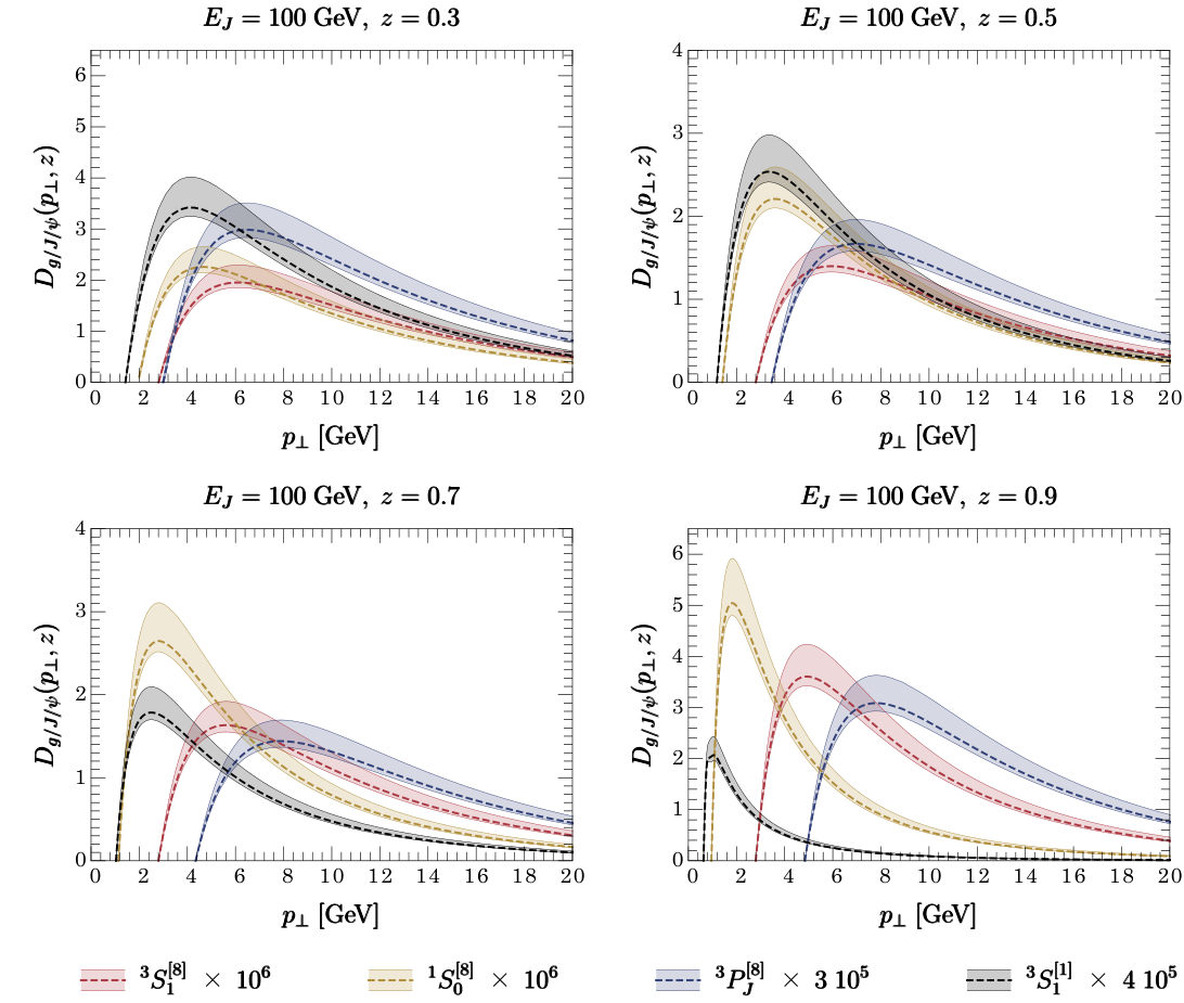
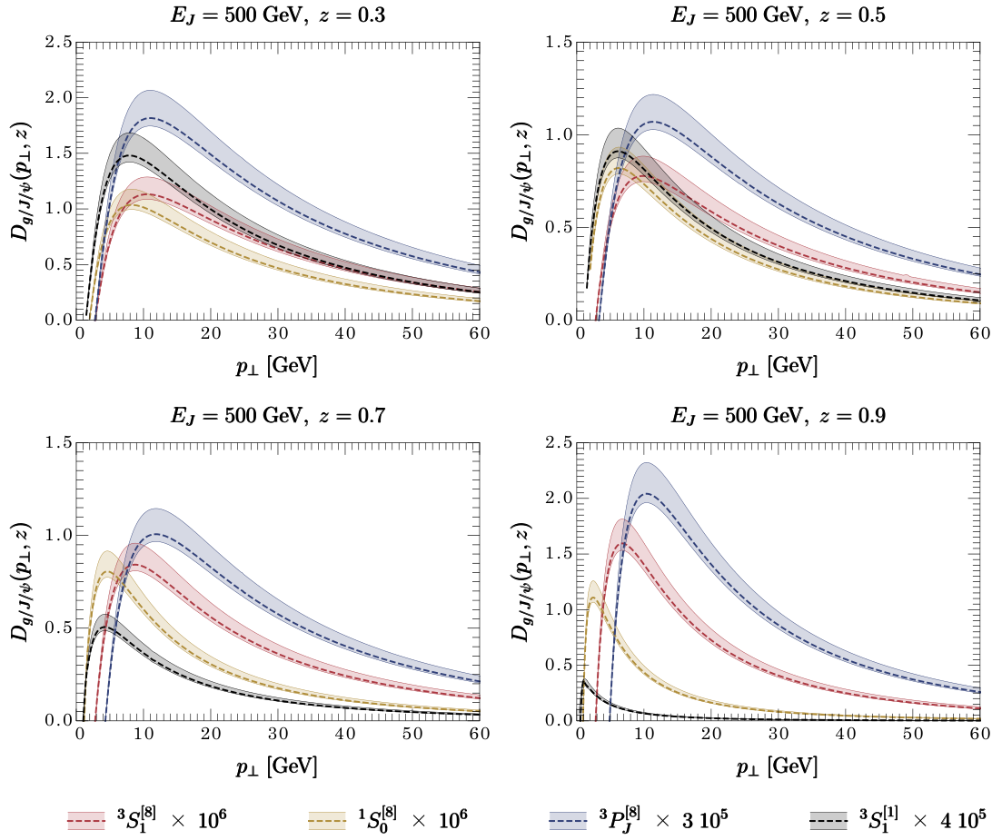
The TMDFJF as a function of for fixed , for and , are shown Figs. 4 and 6, for jet energies of 100 and 500 GeV, respectively. In order to make it easier to view all distributions simultaneously, we have rescaled the , , ,and distributions, by factors of , , and , respectively. The same rescaling factor is used in all eight plots in Figs. 4 and 6, and theoretical uncertainties are calculated by varying the RRG and RG scales by a factor of and . The central dashed lines in the figures correspond to the scale choices and . Though we plot our distributions in the range GeV, it is important that to keep in mind that our calculations are only reliable for GeV.
These plots show that the TMDFJF does in fact provide discriminating power amongst the four mechanisms. For , all four distributions look similar for both GeV and 500 GeV. The distributions peak at roughly the same location and they have same slope for large . For , the color-singlet mechanism and the color-octet mechanism peak at lower values of and fall more steeply with than the and color-octet mechanisms. The mechanism has the peculiar feature that in order to obtain a positive FF we need to have a negative LDME, as is found in the fits of Refs. [49, 50]. The peaks in the distribution for the and mechanisms are at very low where perturbation theory is not reliable. On the other hand, the peaks of the and distributions are at larger values of GeV where perturbation theory can be trusted. The gives a slightly harder distribution than mechanism, and both are significantly harder than the other mechanisms.
It is interesting to study the dependence of the TMDFJF as a function of with fixed to be a perturbative scale. In Fig. 5 we plot the TMDFJF as a function of for GeV for jets with energy 100 and 500 GeV. Large logarithms and shape function effects will affect these distributions in both the and limits, but our calculations should be reliable for intermediate values of . While for the distributions have similar shapes, in the range , the shapes of all four mechanisms are different. The dependence of the TMDFJF for fixed can be used to differentiate between the NRQCD production mechanisms.
The TMDFJF formalism also allows us to calculate the angle at which are produced relative to the jet axis. The average production angle for the is given by
| (51) |
Using the small angle approximation the differential cross section can be written as
| (52) |
Substituting this into Eq. 51 yields
| (53) |
As discussed in Appendix B, the cross section can be factorized into hard, soft and collinear terms in SCET. In general the hard and soft contributions will not cancel because there is a sum over partonic channels in both the numerator and denominator of Eq. 53. However, they will if gluon fragmentation dominates production, then the expression above can be written as
| (54) |
where is the gluon TMDFJF. Fig. 7 the function is plotted at points and for and for with GeV and GeV, respectively. As was done earlier we have fixed the scale . Note the typical angles are small enough that the small angle approximation is justified. The dashed lines in figure show the results of a fit to the functional form, , the values of and for each mechanism at each energy are shown in Table 3. Again we see that differences between the various NRQCD mechanisms become more pronounced as increases. This shows that the average angle does in fact yield some discriminating power between the octet mechanisms. In particular the slope on the semilog plot, which is determined by the parameter in Table 3, differs by as much as 20% between the various NRQCD mechansims for GeV and and as much as 40% for 500 GeV. Note however that and give very similar predictions for this observable.
4 Conclusions
In this paper we introduce the transverse momentum dependent fragmenting jet function (TMDFJF) in the framework of SCET and show how it is related to the previously introduced TMDFFs and fragmenting jet functions (FJFs). TMDFJFs describe the transverse as well as longitudinal momentum distribution of an identified hadron within a jet. TMDFJFs evolve with the renormalization group (RG) scale and obey RG equations similar to jet functions. Using we show that this new distribution can be further factorized into soft and purely collinear terms. The purely collinear factor can be written as a convolution of perturbatively calculable short distance coefficients and the standard FFs, where the soft factor is given by a vacuum matrix element of product of Wilson lines. This factorization introduces rapidity divergences that are regulated with the rapidity regulator. We check that at NLO the regulator dependance vanishes in the final product. Associated with rapidity divergences are rapidity renormalization group (RRG) equations. By evolving the collinear and soft terms separately using the RG and RRG equations all orders resummation of large logarithms in the TMDFJF can be performed.
As an example we implement this formalism for the case of quarkonium production. In the case of quarkonia the TMDFJF can be calculated in terms of the NRQCD FFs which are perturbatively calculable at the scale . For the gluon TMDFJF for , we study the and dependence predicted by the four production mechanisms: , and . We use the leading order (in ) NRQCD FF for each of these mechanisms, and the RG and RRG equations are used to calculate the TMDFJFs to next-to-leading-logarithmic-prime (NLL’) accuracy. We find that the dependence (for fixed ) is different for all four mechanisms. We also find that the dependence on and the average angle of the relative to the jet axis can discriminate between the various NRQCD production mechanisms.
Acknowledgements.
The authors would like to thank Aneesh Manohar for his helpful suggestions on the manuscript. TM and YM are supported in part by the Director, Office of Science, Office of Nuclear Physics, of the U.S. Department of Energy under grant numbers DE-FG02-05ER41368. RB is supported by a National Science Foundation Graduate Research Fellowship under Grant No. 3380012.Appendix A Matching calculation
In this Appendix we provide details for the evaluation of the matching coefficients, . From the sum of diagrams in Figs. 2a) and 2b) we get:
| (55) |
where we define . The superscripts and denote bare and renormalized quantities, respectively, and the superscript indicates that this is the contribution. The NLO matching coefficient is given by
| (56) |
where
| (57) |
The pole appearing in the FF is interpreted as an infrared divergence. Although for extracting the renormalized matching coefficients we can ignore scaleless integrals and interpret the finite terms as the renormalized result to that particular order, here we are interested in the origin of the poles since this will allow us to extract the anomalous dimensions. Performing the matching we get:
| (58) |
For the coefficient we simply perform the replacement and drop and plus-distributions since these functions are always integrated for values of greater than zero. Thus
| (59) |
where . For the gluon splitting we get
| (60) |
Expanding in and we have
| (61) |
and since the corresponding FF is given by:
| (62) |
where the pole is an infrared divergence, we have
| (63) |
A similar calculation yields the kernel ,
| (64) |
where . Performing the matching and since the corresponding FF is
| (65) |
where again the pole is an infrared divergence, we get
| (66) |
Appendix B Factorization Theorems in SCET
Much like the standard FJFs, TMDFJFs appear in factorization theorems for cross-sections that are differential in , the fraction of a jet initiating parton’s energy carried by an identified hadron, and , the transverse momenta of the hadron measured from the parton’s momentum. It is shown in Ref. [48] that the cross-section for the production of two jets in electron-positron annihilation can be written as,
| (67) |
where is the Born cross section, is the hard function resulting from matching a 2-jet operator in full QCD onto the corresponding SCET operators, is a soft function that describes soft scale cross-talk between the jets and the soft out-of-jet radiation is constrained via , and is a jet function that describes collinear radiation within a jet in the direction that has energy (here ). The jet function can be defined in SCET as
| (68) |
To study jets with identified hadrons, we insert the following expression for the identity
| (69) |
| (70) |
where is an identified hadron within the jet. Performing the integration over , which is the Fourier conjugate of the residual momenta, and the residual yields
| (71) |
Insetrting this back to Eq.(67) we have
| (72) |
which directly implies
| (73) |
This suggests a rather powerful rule (already known to be true for the standard FJFs) for constructing the factorization theorem in SCET with identified hadron with measured transverse momenta :
| (74) |
Appendix C Solving the RG and RRG Equations
C.1 RRG Evolution
The RRG equation in momentum space for a renormalized function is given by
| (75) |
where the anomalous dimension can be written in the following generic form,
| (76) |
where
| (77) |
The cusp and non-cusp parts of the anomalous dimension are listed in Table 4. Taking the Fourier transform of Eq. (75) yields,
| (78) |
where the Fourier conjugate of is where and using the form of the anomalous dimensions in Eq. (44,45) gives that,
| (79) |
where . Integrating Eq. (78) yields
| (80) |
where
| (81) |
with
| (82) |
| Function | ||||
|---|---|---|---|---|
C.2 RG Evolution
Evolution in begins with the following RG equation
| (83) |
where the anomalous dimension can be written in the generic form
| (84) |
The coefficient is proportional to the cusp anomalous dimension, , which can be expanded in
| (85) |
and . The non-cusp part, , has a similar expansion
| (86) |
The solultion to the RGE is thus given by
| (87) |
where again
| (88) |
and the exponents and are given in terms of the anomalous dimension,
| (89) | ||||
| (90) |
and for up to NLL and NLL’ accuracy are given by
| (91) | ||||
| (92) |
where and are the coefficients of the QCD -function,
| (93) |
References
- (1) A. Altheimer et al., Boosted objects and jet substructure at the LHC. Report of BOOST2012, held at IFIC Valencia, 23rd-27th of July 2012, Eur. Phys. J. C74 (2014) 2792, [1311.2708].
- (2) S. Sapeta, QCD and Jets at Hadron Colliders, Prog. Part. Nucl. Phys. 89 (2016) 1–55, [1511.09336].
- (3) M. Procura and I. W. Stewart, Quark Fragmentation within an Identified Jet, Phys.Rev. D81 (2010) 074009, [0911.4980].
- (4) C. W. Bauer, D. Pirjol and I. W. Stewart, Soft collinear factorization in effective field theory, Phys. Rev. D65 (2002) 054022, [hep-ph/0109045].
- (5) C. W. Bauer, S. Fleming and M. E. Luke, Summing Sudakov logarithms in in effective field theory, Phys. Rev. D63 (2000) 014006, [hep-ph/0005275].
- (6) C. W. Bauer, S. Fleming, D. Pirjol and I. W. Stewart, An Effective field theory for collinear and soft gluons: Heavy to light decays, Phys. Rev. D63 (2001) 114020, [hep-ph/0011336].
- (7) C. W. Bauer and I. W. Stewart, Invariant operators in collinear effective theory, Phys. Lett. B516 (2001) 134–142, [hep-ph/0107001].
- (8) A. Jain, M. Procura and W. J. Waalewijn, Parton Fragmentation within an Identified Jet at NNLL, JHEP 1105 (2011) 035, [1101.4953].
- (9) X. Liu, SCET approach to top quark decay, Phys.Lett. B699 (2011) 87–92, [1011.3872].
- (10) C. F. Berger, T. Kucs and G. F. Sterman, Event shape / energy flow correlations, Phys. Rev. D68 (2003) 014012, [hep-ph/0303051].
- (11) R. Bain, L. Dai, A. Hornig, A. K. Leibovich, Y. Makris and T. Mehen, Analytic and Monte Carlo Studies of Jets with Heavy Mesons and Quarkonia, JHEP 06 (2016) 121, [1603.06981].
- (12) M. Procura and W. J. Waalewijn, Fragmentation in Jets: Cone and Threshold Effects, Phys.Rev. D85 (2012) 114041, [1111.6605].
- (13) M. Baumgart, A. K. Leibovich, T. Mehen and I. Z. Rothstein, Probing Quarkonium Production Mechanisms with Jet Substructure, JHEP 11 (2014) 003, [1406.2295].
- (14) Y.-T. Chien, Z.-B. Kang, F. Ringer, I. Vitev and H. Xing, Jet fragmentation functions in proton-proton collisions using soft-collinear effective theory, JHEP 05 (2016) 125, [1512.06851].
- (15) A. Jain, M. Procura and W. J. Waalewijn, Fully-Unintegrated Parton Distribution and Fragmentation Functions at Perturbative , JHEP 1204 (2012) 132, [1110.0839].
- (16) A. Jain, M. Procura, B. Shotwell and W. J. Waalewijn, Fragmentation with a Cut on Thrust: Predictions for B-factories, Phys. Rev. D87 (2013) 074013, [1207.4788].
- (17) C. W. Bauer and E. Mereghetti, Heavy Quark Fragmenting Jet Functions, JHEP 04 (2014) 051, [1312.5605].
- (18) L. Dai, C. Kim and A. K. Leibovich, Fragmentation of a Jet with Small Radius, 1606.07411.
- (19) Z.-B. Kang, F. Ringer and I. Vitev, Jet substructure using semi-inclusive jet functions within SCET, 1606.07063.
- (20) M. Ritzmann and W. J. Waalewijn, Fragmentation in Jets at NNLO, Phys.Rev. D90 (2014) 054029, [1407.3272].
- (21) Z.-B. Kang, F. Ringer and I. Vitev, Semi-inclusive jet cross sections within SCET, 2016. 1609.07112.
- (22) A. Metz and A. Vossen, Parton Fragmentation Functions, 1607.02521.
- (23) M. G. Echevarria, A. Idilbi and I. Scimemi, Factorization Theorem For Drell-Yan At Low And Transverse Momentum Distributions On-The-Light-Cone, JHEP 07 (2012) 002, [1111.4996].
- (24) M. G. Echevarria, A. Idilbi, A. Schäfer and I. Scimemi, Model-Independent Evolution of Transverse Momentum Dependent Distribution Functions (TMDs) at NNLL, Eur. Phys. J. C73 (2013) 2636, [1208.1281].
- (25) M. G. Echevarria, A. Idilbi and I. Scimemi, Unified treatment of the QCD evolution of all (un-)polarized transverse momentum dependent functions: Collins function as a study case, Phys. Rev. D90 (2014) 014003, [1402.0869].
- (26) M. G. Echevarria, I. Scimemi and A. Vladimirov, Transverse momentum dependent fragmentation function at next-to-next-to-leading order, Phys. Rev. D93 (2016) 011502, [1509.06392].
- (27) M. G. Echevarria, I. Scimemi and A. Vladimirov, Unpolarized Transverse Momentum Dependent Parton Distribution and Fragmentation Functions at next-to-next-to-leading order, 1604.07869.
- (28) M. Anselmino, M. Boglione, J. O. Gonzalez Hernandez, S. Melis and A. Prokudin, Unpolarised Transverse Momentum Dependent Distribution and Fragmentation Functions from SIDIS Multiplicities, JHEP 04 (2014) 005, [1312.6261].
- (29) M. Procura, W. J. Waalewijn and L. Zeune, Resummation of Double-Differential Cross Sections and Fully-Unintegrated Parton Distribution Functions, JHEP 02 (2015) 117, [1410.6483].
- (30) B. U. Musch, P. Hagler, J. W. Negele and A. Schafer, Exploring quark transverse momentum distributions with lattice QCD, Phys. Rev. D83 (2011) 094507, [1011.1213].
- (31) J.-Y. Chiu, A. Jain, D. Neill and I. Z. Rothstein, A Formalism for the Systematic Treatment of Rapidity Logarithms in Quantum Field Theory, JHEP 1205 (2012) 084, [1202.0814].
- (32) D. Neill, I. Z. Rothstein and V. Vaidya, The Higgs Transverse Momentum Distribution at NNLL and its Theoretical Errors, JHEP 12 (2015) 097, [1503.00005].
- (33) T. Lübbert, J. Oredsson and M. Stahlhofen, Rapidity renormalized TMD soft and beam functions at two loops, JHEP 03 (2016) 168, [1602.01829].
- (34) T. Becher, M. Neubert and D. Wilhelm, Higgs-Boson Production at Small Transverse Momentum, JHEP 05 (2013) 110, [1212.2621].
- (35) T. Becher, M. Neubert and D. Wilhelm, Electroweak gauge-boson and Higgs production at Small : Infrared safety from the collinear anomaly, in Proceedings, 20th International Workshop on Deep-Inelastic Scattering and Related Subjects (DIS 2012): Bonn, Germany, March 26-30, 2012, pp. 721–724, 2012. DOI.
- (36) V. Ahrens, T. Becher, M. Neubert and L. L. Yang, Renormalization-Group Improved Prediction for Higgs Production at Hadron Colliders, Eur. Phys. J. C62 (2009) 333–353, [0809.4283].
- (37) C. W. Bauer, F. J. Tackmann, J. R. Walsh and S. Zuberi, Factorization and Resummation for Dijet Invariant Mass Spectra, Phys. Rev. D85 (2012) 074006, [1106.6047].
- (38) Y.-T. Chien, A. Hornig and C. Lee, Soft-collinear mode for jet cross sections in soft collinear effective theory, Phys. Rev. D93 (2016) 014033, [1509.04287].
- (39) P. Pietrulewicz, F. J. Tackmann and W. J. Waalewijn, Factorization and Resummation for Generic Hierarchies between Jets, 1601.05088.
- (40) G. T. Bodwin, E. Braaten and G. P. Lepage, Rigorous QCD analysis of inclusive annihilation and production of heavy quarkonium, Phys. Rev. D51 (1995) 1125–1171, [hep-ph/9407339].
- (41) E. Braaten, K.-m. Cheung and T. C. Yuan, Z0 decay into charmonium via charm quark fragmentation, Phys. Rev. D48 (1993) 4230–4235, [hep-ph/9302307].
- (42) E. Braaten and T. C. Yuan, Gluon fragmentation into heavy quarkonium, Phys. Rev. Lett. 71 (1993) 1673–1676, [hep-ph/9303205].
- (43) E. Braaten and S. Fleming, Color octet fragmentation and the psi-prime surplus at the Tevatron, Phys. Rev. Lett. 74 (1995) 3327–3330, [hep-ph/9411365].
- (44) E. Braaten and Y.-Q. Chen, Helicity decomposition for inclusive J / psi production, Phys. Rev. D54 (1996) 3216–3227, [hep-ph/9604237].
- (45) J. C. Collins and D. E. Soper, Parton Distribution and Decay Functions, Nucl. Phys. B194 (1982) 445–492.
- (46) S. M. Aybat and T. C. Rogers, TMD Parton Distribution and Fragmentation Functions with QCD Evolution, Phys. Rev. D83 (2011) 114042, [1101.5057].
- (47) J.-y. Chiu, A. Jain, D. Neill and I. Z. Rothstein, The Rapidity Renormalization Group, Phys. Rev. Lett. 108 (2012) 151601, [1104.0881].
- (48) S. D. Ellis, C. K. Vermilion, J. R. Walsh, A. Hornig and C. Lee, Jet Shapes and Jet Algorithms in SCET, JHEP 11 (2010) 101, [1001.0014].
- (49) M. Butenschoen and B. A. Kniehl, World data of J/psi production consolidate NRQCD at NLO, Phys. Rev. D84 (2011) 051501, [1105.0820].
- (50) M. Butenschoen and B. A. Kniehl, Next-to-leading-order tests of NRQCD factorization with yield and polarization, Mod. Phys. Lett. A28 (2013) 1350027, [1212.2037].