跳到论文正文
W Papers独立论文阅读器 arXiv:1610.06469 论文正文 计算阅读时间 · 0%
引用这篇论文根据当前论文元数据生成,正式投稿前建议核对。


License: arXiv.org perpetual non-exclusive license
arXiv:1610.06469v2 [math.NA] 02 Oct 2017

Fast and guaranteed blind multichannel deconvolution under a bilinear system model

Kiryung Lee    Ning Tian    Justin Romberg ††thanks: This work was supported in part by NSF grants CCF 14-22540, IIS 14-47879, and by ONR grant N00014-13-1-0632.††thanks: An earlier version of this work was presented in part at the 2016 IEEE Information Theory Workshop [1] and the 22nd International Conference on Digital Signal Processing [2].††thanks: The authors are with the School of Electrical and Computer Engineering, Georgia Institute of Technology, Atlanta, GA 30332, USA (e-mail: {kiryung,jrom}@ece.gatech.edu, ningtian@gatech.edu).
Abstract

We consider the multichannel blind deconvolution problem where we observe the output of multiple channels that are all excited with the same unknown input. From these observations, we wish to estimate the impulse responses of each of the channels. We show that this problem is well-posed if the channels follow a bilinear model where the ensemble of channel responses is modeled as lying in a low-dimensional subspace but with each channel modulated by an independent gain. Under this model, we show how the channel estimates can be found by minimizing a quadratic functional over a non-convex set.

We analyze two methods for solving this non-convex program, and provide performance guarantees for each. The first is a method of alternating eigenvectors that breaks the program down into a series of eigenvalue problems. The second is a truncated power iteration, which can roughly be interpreted as a method for finding the largest eigenvector of a symmetric matrix with the additional constraint that it adheres to our bilinear model. As with most non-convex optimization algorithms, the performance of both of these algorithms is highly dependent on having a good starting point. We show how such a starting point can be constructed from the channel measurements.

Our performance guarantees are non-asymptotic, and provide a sufficient condition on the number of samples observed per channel in order to guarantee channel estimates of a certain accuracy. Our analysis uses a model with a “generic” subspace that is drawn at random, and we show the performance bounds hold with high probability. Mathematically, the key estimates are derived by quantifying how well the eigenvectors of certain random matrices approximate the eigenvectors of their mean.

We also present a series of numerical results demonstrating that the empirical performance is consistent with the presented theory.

Index Terms: 
Blind deconvolution, non-convex optimization, eigenvalue decomposition, sensitivity analysis.

I Introduction

Blind deconvolution, where we estimate two unknown signals from an observation of their convolution, is a classical problem in signal processing. It is ubiquitous, appearing in applications including channel estimation in communications, image deblurring and restoration, seismic data analysis, speech dereverberation, medical imaging, and convolutive dictionary learning. While algorithms based on heuristics for particular applications have existed for decades, it is not until recently that a rich mathematical theory has developed around this problem. The fundamental identifiability of solutions to this problem has been studied from an information theoretic perspective [3, 4, 5, 6, 7, 8, 9]. Practical algorithms with provable performance guarantees that make the problem well-posed by imposing structural constraints on the signals have arisen based on ideas from compressed sensing and low-rank matrix recovery. These include methods based on convex programming [10, 11, 12], alternating minimization [13], and gradient descent [14]. More recent works studied the more challenging problem of blind deconvolution with off-the-grid sparsity models [15, 16].

In this paper, we consider the multichannel blind deconvolution problem: we observe a single unknown signal (the “source”) convolved with a number of different “channels”. The fact that the input is shared makes this problem better-posed than in the single channel case. Mathematical theory for the multichannel problem under various constraints has existed since the 1990s (see [17, 18] for surveys). One particular strand of this research detailed in [19, 20, 21] gives concrete results under the very loose assumption that the channel responses are time-limited. These works show how with this model in place, the channel responses can be estimated by forming a cross-correlation matrix from the channel outputs and then computing its smallest eigenvector. This estimate is consistent in that it is guaranteed to converge to the true channel responses as the number of observations gets infinitely large. However, no performance guarantees were given for a finite number of samples, and the method tends to be unstable for moderate sample values in even modest noise. Recent work [22] has shown that this spectral method can indeed be stabilized by introducing a more restrictive linear (subspace) model on the channel responses.

Our main contributions in this paper are methods for estimating the channel responses when the ensemble has a certain kind of bilinear structure. In particular, we model the ensemble of channel responses as lying in a low-dimensional subspace, but with each channel modulated by an independent constant; we will discuss in the next section an application in which this model is relevant. Our estimation framework again centers on constructing a cross-correlation matrix and minimizing a quadratic functional involving this matrix over the unit sphere, but with the additional constraint that the solution can be written as the Kronecker product of two shorter vectors. This optimization program, which might be interpreted as a kind of structured eigenvalue problem, is inherently non-convex. We propose two iterative methods for solving it, each with very simple, computationally efficient iterations. The first is a method of alternating eigenvectors, where we alternate between fixing a subset of the unknowns and estimating the other by solving a standard eigenvalue problem. The second method is a truncated power iteration, where we repeatedly apply the cross-correlation matrix to an initial point, but project the result after each application to enforce the structural constraints. We derive performance guarantees for both of these algorithms when the low-dimensional subspace is generic (i.e. generated at random).

Related work

Closely related to the problem of multichannel blind deconvolution is the problem of blind calibration. Here we observe the product of an unknown weighting vector applied to a series of other unknown vectors. Non-convex optimization algorithms for blind calibration have been studied and analyzed in [23, 24].

Multichannel blind deconvolution can also be approached by linearizing the problem in the Fourier domain. This has been proposed for various applications, including the calibration of a sensor network [25], computational relighting in inverse rendering [26], and auto-focus in synthetic aperture radar [27]. Under a generic condition that the unknown impulse responses belong to random subspaces, necessary and sufficient conditions for the unique identification of the solution have been put forth in [6], and a rigorous analysis of a least-squares method has been studied [28].

More recently, performance guarantees for spectral methods for for both subspace and sparsity models have been developed in [29]. As in this paper, these methods are estimating the channel by solving a structured eigenvalue problem. The structural model, however, is very different than the one considered here.

Algorithms for solving non-convex quadratic and bilinear problems have recently been introduced for solving problems closely related to blind deconvolution. A non-convex optimization over matrix manifolds provides a guaranteed solution for matrix completion [30]. Alternating minimization is another non-convex optimization algorithm for matrix completion that provides a provable performance guarantee [31, 32, 33]. Yet for another example, a suite of gradient-based algorithms with a specially designed regularizer within the conventional Euclidean geometry have been studied recently [34]. Phase retrieval is cast as a non-convex optimization due to the nonlinearity in generating the observation. Wirtinger flow algorithms [35, 36, 37, 38] and alternating minimization [39, 40] are non-convex optimization algorithms for the phase retrieval problem. Dictionary learning is another bilinear problem arising in numerous applications. Convergence of a Riemannian trust-region method for dictionary learning has been studied with a thorough geometric analysis [41, 42]. On the other hand, although it provides the convergence analysis of different nature, convergence of an alternating minimization for blind Ptychographic diffraction imaging to a local minima regardless of the initial point has been shown under a mild condition [43].

Organization

The rest of this paper is organized as follows. The multichannel blind deconvolution problem is formulated under a bilinear channel model in Section II. After we review relevant previous methods for multichannel blind deconvolution in Section III, we present two iterative algorithms for multichannel blind deconvolution under the bilinear channel model in Section IV, which are obtained by modifying the classical cross-convolution method. Our main results on non-asymptotic stable recovery are presented in Section V with an outline of the proofs. Detailed analysis of the spectral initialization and the two iterative algorithms are derived in Sections VII, VIII, and IX. We demonstrate numerical results that support our theory in Section VI, and summarize our conclusions in Section X.

II Problem Statement

In the classic multichannel blind deconvolution problem, we observe an unknown signal 𝒙∈ℂL\bm{x}\in\mathbb{C}^{L} that has been convolved with MM different unknown channel responses 𝒉1,…,𝒉m∈ℂL\bm{h}_{1},\ldots,\bm{h}_{m}\in\mathbb{C}^{L}:

𝒚m=𝒉m⊛𝒙+𝒘m,m=1,…,M,\bm{y}_{m}=\bm{h}_{m}\circledast\bm{x}+\bm{w}_{m},\quad m=1,\dots,M, (1)

where ⊛\circledast denotes circular convolution11 1 We are using circular convolution in our model problem for the ease of analysis. modulo LL and 𝒘m∈ℂL\bm{w}_{m}\in\mathbb{C}^{L} denotes additive noise. Given the outputs {𝒚m}m=1M\{\bm{y}_{m}\}_{m=1}^{M}, and working without knowledge of the common input 𝒙\bm{x}, we want to recover the unknown channel impulse responses {𝒉m}m=1M\{\bm{h}_{m}\}_{m=1}^{M}.

We will show how we can solve this problem when the channels are time-limited, and obey a bilinear model. By time-limited, we mean that only the first KK entries in the 𝒉m\bm{h}_{m} can be non-zero; we can write

𝒉m=𝑺⊤​𝒉¯m,where𝑺:=[𝐈K𝟎K,L−K].\bm{h}_{m}=\bm{S}^{\top}\underline{\bm{h}}_{m},\quad\text{where}\quad\bm{S}:=\begin{bmatrix}{\bf I}_{K}&\bm{0}_{K,L-K}\end{bmatrix}. (2)

In addition, the 𝒉m\bm{h}_{m} are jointly modeled as lying in a DD-dimensional subspace of ℂK\mathbb{C}^{K}, but are modulated by unknown channel gains a1,…,aM>0a_{1},\ldots,a_{M}>0. This means that

𝒉¯m=am𝚽m𝒃,∀m=1,…,M,\underline{\bm{h}}_{m}=a_{m}\bm{\Phi}_{m}\bm{b},\quad\forall m=1,\dots,M, (3)

where the 𝚽m\bm{\Phi}_{m} are complex K×DK\times D matrices, whose columns span are the parts of the basis vectors corresponding to channel mm, and 𝒃∈ℂD\bm{b}\in\mathbb{C}^{D} is the common set of basis coefficients. Stacking up the channel responses into a single vector 𝒉¯∈ℂM​K\underline{\bm{h}}\in\mathbb{C}^{MK} and the gains into 𝒂∈ℂM\bm{a}\in\mathbb{C}^{M}, an equivalent way to write (3) is

𝒉¯=𝚽⁡(𝒂⊗𝒃),where𝚽:=[ 𝟎​ ⋮​ 𝟎​𝚽1​    𝟎​ ⋮​ 𝚽2​𝟎​    …​ ⋱​ …​…​    𝚽M​ ⋮​ 𝟎​𝟎​   ]​and𝒂⊗𝒃=[a1​𝒃a2​𝒃aM​𝒃].\underline{\bm{h}}=\bm{\Phi}(\bm{a}\otimes\bm{b}),\quad\text{where}\quad\bm{\Phi}:=\left[\ignorespaces\ignorespaces\ignorespaces\ignorespaces\ignorespaces\ignorespaces\ignorespaces\ignorespaces\ignorespaces\ignorespaces\ignorespaces\ignorespaces\ignorespaces\ignorespaces\ignorespaces\ignorespaces\ignorespaces\ignorespaces\ignorespaces\ignorespaces\ignorespaces\ignorespaces\ignorespaces\ignorespaces\ignorespaces{\ignorespaces\ignorespaces\ignorespaces\ignorespaces\ignorespaces\ignorespaces\makebox[17.18192pt][c]{\raisebox{-3.43056pt}{\hbox{\ignorespaces\ignorespaces\ignorespaces\ignorespaces\ignorespaces\ignorespaces\ignorespaces\ignorespaces\ignorespaces\hbox{\hskip 6.39581pt\hskip-2.87498pt\hbox{$\ignorespaces\bm{0}\rule[-2.0pt]{0.0pt}{9.0pt}$}\hskip-2.87498pt\hskip-6.39581pt\raisebox{13.20007pt}{$\hbox{\hskip 6.39581pt\hskip 0.0pt\hbox{$\ignorespaces\vdots\rule[-2.0pt]{0.0pt}{9.0pt}$}\hskip 0.0pt\hskip-6.39581pt\raisebox{13.20007pt}{$\hbox{\hskip 6.39581pt\hskip-2.87498pt\hbox{$\ignorespaces\bm{0}\rule[-2.0pt]{0.0pt}{9.0pt}$}\hskip-2.87498pt\hskip-6.39581pt\raisebox{13.20007pt}{$\hbox{$\ignorespaces\bm{\Phi}_{1}\rule[-2.0pt]{0.0pt}{9.0pt}$}$}\hskip-6.39581pt\hskip 6.39581pt}$}\hskip-6.39581pt\hskip 6.39581pt}$}\hskip-6.39581pt\hskip 6.39581pt}}}}\ignorespaces\ignorespaces\hskip 0.0pt\ignorespaces\ignorespaces\ignorespaces\ignorespaces\makebox[17.18192pt][c]{\raisebox{-3.43056pt}{\hbox{\ignorespaces\ignorespaces\ignorespaces\ignorespaces\ignorespaces\ignorespaces\ignorespaces\ignorespaces\ignorespaces\hbox{\hskip 6.39581pt\hskip-2.87498pt\hbox{$\ignorespaces\bm{0}\rule[-2.0pt]{0.0pt}{9.0pt}$}\hskip-2.87498pt\hskip-6.39581pt\raisebox{13.20007pt}{$\hbox{\hskip 6.39581pt\hskip 0.0pt\hbox{$\ignorespaces\vdots\rule[-2.0pt]{0.0pt}{9.0pt}$}\hskip 0.0pt\hskip-6.39581pt\raisebox{13.20007pt}{$\hbox{\hskip 6.39581pt\hskip-6.39581pt\hbox{$\ignorespaces\bm{\Phi}_{2}\rule[-2.0pt]{0.0pt}{9.0pt}$}\hskip-6.39581pt\hskip-2.87498pt\raisebox{13.20007pt}{$\hbox{$\ignorespaces\bm{0}\rule[-2.0pt]{0.0pt}{9.0pt}$}$}\hskip-2.87498pt\hskip 6.39581pt}$}\hskip-6.39581pt\hskip 6.39581pt}$}\hskip-6.39581pt\hskip 6.39581pt}}}}\ignorespaces\ignorespaces\hskip 0.0pt\ignorespaces\ignorespaces\ignorespaces\ignorespaces\makebox[17.18192pt][c]{\raisebox{-3.5pt}{\hbox{\ignorespaces\ignorespaces\ignorespaces\ignorespaces\ignorespaces\ignorespaces\ignorespaces\ignorespaces\ignorespaces\hbox{\hskip 3.75pt\hskip-3.75pt\hbox{$\ignorespaces\dots\rule[-2.0pt]{0.0pt}{9.0pt}$}\hskip-3.75pt\hskip-3.75pt\raisebox{13.20007pt}{$\hbox{\hskip 3.75pt\hskip-3.75pt\hbox{$\ignorespaces\ddots\rule[-2.0pt]{0.0pt}{9.0pt}$}\hskip-3.75pt\hskip-3.75pt\raisebox{13.20007pt}{$\hbox{\hskip 3.75pt\hskip-3.75pt\hbox{$\ignorespaces\dots\rule[-2.0pt]{0.0pt}{9.0pt}$}\hskip-3.75pt\hskip-3.75pt\raisebox{13.20007pt}{$\hbox{$\ignorespaces\dots\rule[-2.0pt]{0.0pt}{9.0pt}$}$}\hskip-3.75pt\hskip 3.75pt}$}\hskip-3.75pt\hskip 3.75pt}$}\hskip-3.75pt\hskip 3.75pt}}}}\ignorespaces\ignorespaces\hskip 0.0pt\ignorespaces\ignorespaces\ignorespaces\ignorespaces\makebox[17.18192pt][c]{\raisebox{-3.43056pt}{\hbox{\ignorespaces\ignorespaces\ignorespaces\ignorespaces\ignorespaces\ignorespaces\ignorespaces\ignorespaces\ignorespaces\hbox{\hskip 8.59096pt\hskip-8.59096pt\hbox{$\ignorespaces\bm{\Phi}_{M}\rule[-2.0pt]{0.0pt}{9.0pt}$}\hskip-8.59096pt\hskip-2.87498pt\raisebox{13.20007pt}{$\hbox{\hskip 2.87498pt\hskip 0.0pt\hbox{$\ignorespaces\vdots\rule[-2.0pt]{0.0pt}{9.0pt}$}\hskip 0.0pt\hskip-2.87498pt\raisebox{13.20007pt}{$\hbox{\hskip 2.87498pt\hskip-2.87498pt\hbox{$\ignorespaces\bm{0}\rule[-2.0pt]{0.0pt}{9.0pt}$}\hskip-2.87498pt\hskip-2.87498pt\raisebox{13.20007pt}{$\hbox{$\ignorespaces\bm{0}\rule[-2.0pt]{0.0pt}{9.0pt}$}$}\hskip-2.87498pt\hskip 2.87498pt}$}\hskip-2.87498pt\hskip 2.87498pt}$}\hskip-2.87498pt\hskip 8.59096pt}}}}\ignorespaces}\right]~~\text{and}\quad\bm{a}\otimes\bm{b}=\begin{bmatrix}a_{1}\bm{b}\\ a_{2}\bm{b}\\ \vdots\\ a_{M}\bm{b}\end{bmatrix}. (4)

This alternative expression can be interpreted as a linear subspace model with respect to the basis 𝚽∈ℂM​K×M​D\bm{\Phi}\in\mathbb{C}^{MK\times MD} with a separability (rank-1) prior on the coefficient vector.
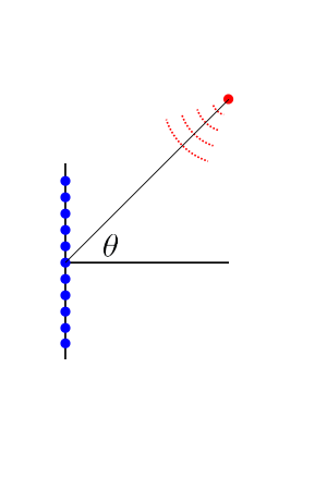
Refer to caption
(a)
Refer to caption
(b)
(c)
Refer to caption
(d)
Fig. 1: Illustration of construction of a joint linear subspace model from a parametric model. A uniform array of MM sensors. Examples of {𝒈r→}\{\bm{g}_{\vec{r}}\} rearranged as MM-by-KK matrices. Sorted eigenvalues of 𝑯ℛ\bm{H}_{\mathcal{R}} in a logarithmic scale. First few dominant eigenvectors of 𝑯ℛ\bm{H}_{\mathcal{R}} rearranged as MM-by-KK matrices.

For an example of how a model like this might arise, we consider the following stylized problem for array processing illustrated in Figure 1. Figure  shows a linear array. Suppose we know that if a source is at location r→\vec{r} then the concatenation of the channel responses between that source location and the array elements is 𝒈r→∈ℂM​K\bm{g}_{\vec{r}}\in\mathbb{C}^{MK}. In simple environments, these channel responses might look very similar to one another in that they are all (sampled) versions of the same shifted function (See Figure ). The delays are induced by the differences in sensor locations relative to the source, while the shape of the response might be determined by the instrumentation used to take the measurements (e.g. the frequency response of the sensors) — there could even be small differences in this shape from element to element.

Suppose now that there is uncertainty in the source location that we model as r→∈ℛ\vec{r}\in\mathcal{R}, where ℛ\mathcal{R} is some region in space. As we vary r→\vec{r} over the set ℛ\mathcal{R}, the responses 𝒈r→\bm{g}_{\vec{r}} trace out a portion of a manifold in ℂM​K\mathbb{C}^{MK}. We can (approximately) embed this manifold in a linear subspace of dimension DD by looking at the DD principal eigenvectors of the matrix

𝑯ℛ=∫r→∈ℛ𝒈r→​𝒈r→∗​𝑑r→.\bm{H}_{\mathcal{R}}=\int_{\vec{r}\in\mathcal{R}}\bm{g}_{\vec{r}}\,\bm{g}_{\vec{r}}^{*}~d\vec{r}.

The dimension DD that allows an accurate embedding will depend on the size of ℛ\mathcal{R} and smoothness properties of the mapping from r→\vec{r} to 𝒈r→\bm{g}_{\vec{r}}. In this case, we are building 𝚽\bm{\Phi} above by taking the M​K×DMK\times D matrix that has the principal eigenvectors as columns and apportioning the first KK rows to 𝚽1\bm{\Phi}_{1}, the next KK rows to 𝚽2\bm{\Phi}_{2}, etc.

This technique of embedding a parametric model into a linear space has been explored for source localization and channel estimation in underwater acoustics in [44, 45], and some analysis in the context of compressed sensing is provided in [46]. However, it is not robust in one important way. In practice, the gains (the amplitude of the channel response) can vary between elements in the array, and this variation is enough to compromise the subspace embedding described above. The bilinear model (4) explicitly accounts for these channel-to-channel variations.

In this paper, we are interested in when equations of the form (1) can be solved for 𝒉m\bm{h}_{m} with the structural constraint (4); we present two different algorithms for doing so in the sections below. These effective of these algorithms will of course affected by properties of 𝚽\bm{\Phi} (including the number of channels MM and embedding dimension DD) as well as the number of samples LL. While empirical models like the one described above are used in practice (see in particular [45]), we will analyze generic instances of this problem, where the linear model is drawn at random.

III Spectral Methods for Multichannel Blind Deconvolution

A classical method for treating the multichannel blind deconvolution problem is to recast it as an eigenvalue problem: we create a correlation matrix using the measured data {𝒚m}\{\bm{y}_{m}\}, and estimate the channels from the smallest eigenvector22 2 By which mean the eigenvector corresponding to the smallest eigenvalue. of this matrix. These methods were pioneered in the mid-1990s in [19, 20, 21], and we briefly review the central ideas in this section. The methods we present in the next section operate on the same basic principles, but explicitly enforce structural constraints on the solution.

The cross-convolution method for multichannel blind deconvolution [19] follows directly from the commutivity of the convolution operator. If there is no noise in the observations (1), then it must be the case that

𝒚m1⊛𝒉m2−𝒚m2⊛𝒉m1=𝟎,for allm1,m2=1,…,M.\bm{y}_{m_{1}}\circledast\bm{h}_{m_{2}}-\bm{y}_{m_{2}}\circledast\bm{h}_{m_{1}}=\bm{0},\quad\text{for all}\quad m_{1},m_{2}=1,\ldots,M.

Using 𝑻𝒚m\bm{T}_{\bm{y}_{m}} as the matrix whose action is convolution with 𝒚m\bm{y}_{m} with a signal of length KK, we see that the channel responses 𝒉m1\bm{h}_{m_{1}} and 𝒉m2\bm{h}_{m_{2}} must obey the linear constraints 𝑻𝒚m1​𝒉¯m2−𝑻𝒚m2​𝒉¯m1=𝟎\bm{T}_{\bm{y}_{m_{1}}}\underline{\bm{h}}_{m_{2}}-\bm{T}_{\bm{y}_{m_{2}}}\underline{\bm{h}}_{m_{1}}=\bm{0}. We can collect all pairs of these linear constraints into a large system, expressed as

𝒀​𝒉¯=𝟎M⁡(M−1)​L/2,1,\bm{Y}\underline{\bm{h}}=\bm{0}_{M(M-1)L/2,1}, (5)

where 𝒀∈ℂM⁡(M−1)​L/2×M​K\bm{Y}\in\mathbb{C}^{M(M-1)L/2\times MK} is defined by

𝒀=[𝒀(1)𝒀(2)𝒀(M−1)],𝒀(i)=[𝟎L,K…𝟎L,K𝟎L,K…𝟎L,K⏟(i−1) blocks𝑻𝒚i+1−𝑻𝒚i⋱𝑻𝒚M−𝑻𝒚i⏟(M−i+1) blocks].\bm{Y}=\begin{bmatrix}\bm{Y}^{(1)}\\ \bm{Y}^{(2)}\\ \vdots\\ \bm{Y}^{(M-1)}\end{bmatrix},\quad\bm{Y}^{(i)}=\begin{bmatrix}\underbrace{\begin{matrix}\bm{0}_{L,K}&\dots&\bm{0}_{L,K}\\ \vdots&&\vdots\\ \bm{0}_{L,K}&\dots&\bm{0}_{L,K}\end{matrix}}_{\text{$(i-1)$ blocks}}&\underbrace{\begin{matrix}\bm{T}_{\bm{y}_{i+1}}&-\bm{T}_{\bm{y}_{i}}&&\\ \vdots&&\ddots&\\ \bm{T}_{\bm{y}_{M}}&&&-\bm{T}_{\bm{y}_{i}}\end{matrix}}_{\text{$(M-i+1)$ blocks}}\end{bmatrix}. (6)

It is shown in [19, 21] that 𝒉¯\underline{\bm{h}} is uniquely determined up to a scaling by (5) (i.e. 𝒀\bm{Y} has a null space that is exactly 11 dimensional) under the mild algebraic condition that the polynomials generated by the (𝒉¯m)m=1M(\underline{\bm{h}}_{m})_{m=1}^{M} have no common zero. In the presence of noise, 𝒉¯\underline{\bm{h}} is estimated as the minimum eigenvector of 𝒀∗​𝒀\bm{Y}^{*}\bm{Y}:

𝒉¯^=arg⁡min‖𝒈‖2=1​𝒈∗​𝒀∗​𝒀​𝒈.\hat{\underline{\bm{h}}}=\arg\min_{\|\bm{g}\|_{2}=1}~\bm{g}^{*}\bm{Y}^{*}\bm{Y}\bm{g}. (7)

Note that 𝒀∗​𝒀\bm{Y}^{*}\bm{Y} is computed cross-correlating the outputs. Therefore, 𝒀∗​𝒀\bm{Y}^{*}\bm{Y} is computed at a low computational cost using the fast Fourier transform. Furthermore, the size of 𝒀∗​𝒀\bm{Y}^{*}\bm{Y}, which is M​K×M​KMK\times MK, does not grow with as the length of observation increases. When there is white additive noise, this cross-correlation matrix will in expectation be the noise-free version plus a scaled identity. These means that as the sample size gets large, the noise and noise-free cross-correlations will have the same eigenvectors, and the estimate (7) is consistent.

A similar technique can be used if we have a linear model for the channel responses, h¯=𝚽​𝒖\underline{h}=\bm{\Phi}\bm{u}. We can estimate the expansion coefficients 𝒖\bm{u} by solving

minimize𝐯⁡𝐯∗​𝚽∗​(𝐘∗​𝐘−ϱ​𝐈)​𝚽​𝐯subject to‖𝐯‖2=1,\minimize_{\bm{v}}~\bm{v}^{*}\bm{\Phi}^{*}\left(\bm{Y}^{*}\bm{Y}-\varrho{\bf I}\right)\bm{\Phi}\bm{v}\quad\text{subject to}\quad\|\bm{v}\|_{2}=1, (8)

where ϱ\varrho is a scalar that depends on the variance of the additive noise (this correction is made so that eigenstructure more closely matches that of 𝚽∗​𝒀∗​𝒀​𝚽\bm{\Phi}^{*}\bm{Y}^{*}\bm{Y}\bm{\Phi} for noise-free 𝒀\bm{Y}). In [22], it was shown that a linear model can significantly improve the stability of the estimate of 𝒉¯\underline{\bm{h}} in the presence of noise, and gave a rigorous non-asymptotic analysis of the estimation error for generic bases 𝚽\bm{\Phi}.

IV Non-convex Optimization Algorithms

Our proposed framework is to solve an optimization program similar to (7) and (8) above, but with the additional constraint that 𝒉¯\underline{\bm{h}} obey the bilinear form (4).

Given the noisy measurements {𝒚m}\{\bm{y}_{m}\} in (1), we create the matrix

𝑨=𝚽∗​(𝒀∗​𝒀−σ^w2​(M−1)​L​𝐈M​K)​𝚽,\bm{A}=\bm{\Phi}^{*}(\bm{Y}^{*}\bm{Y}-\hat{\sigma}_{w}^{2}(M-1)L{\bf I}_{MK})\bm{\Phi},

where σ^w2\hat{\sigma}_{w}^{2} is an estimate of the noise variance σw2\sigma_{w}^{2} (we will briefly discuss how to estimate the noise variance at the end of this section), and 𝒀\bm{Y} is formed as in (6) in the previous section. We then solve a program that is similar to the eigenvalue problems above, but with a Kronecker product constraint on the expansion coefficients:

minimize𝐯,𝐜,𝐝⁡𝐯∗​𝐀𝐯subject to‖𝐯‖2=1,𝐯=𝐜⊗𝐝.\minimize_{\bm{v},\bm{c},\bm{d}}~\bm{v}^{*}\bm{A}\bm{v}\quad\text{subject to}\quad\|\bm{v}\|_{2}=1,\quad\bm{v}=\bm{c}\otimes\bm{d}. (9)

The norm and bilinear constraints make this a non-convex optimization program, and unlike the spectral methods discussed in the last section, there is no (known) computationally efficient algorithm to compute its solution.

We propose and analyze two non-convex optimization algorithms below for solving (9). The first is an alternating eigenvalue method, which iterates between minimizing for 𝒄\bm{c} in (9) with 𝒅\bm{d} fixed, then 𝒅\bm{d} with 𝒄\bm{c} fixed. The second is a variation on the truncated power method [47], whose iterations consist of applications of the matrix 𝑨\bm{A} (just like the standard power method) followed by a projection to enforce the structural constraints.

The performance of both of these methods relies critically on constructing a suitable starting point. We discuss one method for doing so below, then establish its efficacy in Proposition V.7 in Section V-B below.

Alternating eigenvectors. While program (9) is non-convex, it becomes tractable if either of the terms in the tensor constraint are held constant. If we have an estimate 𝒃^\widehat{\bm{b}} for 𝒃\bm{b}, and fix 𝒅=𝒃^\bm{d}=\widehat{\bm{b}}, then we can solve for the optimal 𝒄\bm{c} with

minimize𝐜⁡𝐜∗​𝐀𝐛^​𝐜subject to‖𝐜‖2=1,\minimize_{\bm{c}}~\bm{c}^{*}\bm{A}_{\widehat{\bm{b}}}\bm{c}\quad\text{subject to}\quad\|\bm{c}\|_{2}=1,

where

𝑨𝒃^=(𝐈M⊗𝒃^)∗​𝑨​(𝐈M⊗𝒃^),𝐈M⊗𝒃^=[ 𝟎​ ⋮​ 𝟎​𝒃^​    𝟎​ ⋮​ 𝒃^​𝟎​    …​ ⋱​ …​…​    𝒃^​ ⋮​ 𝟎​𝟎​   ].\bm{A}_{\widehat{\bm{b}}}=({\bf I}_{M}\otimes\hat{\bm{b}})^{*}\bm{A}({\bf I}_{M}\otimes\hat{\bm{b}}),\quad{\bf I}_{M}\otimes\hat{\bm{b}}=\left[\ignorespaces\ignorespaces\ignorespaces\ignorespaces\ignorespaces\ignorespaces\ignorespaces\ignorespaces\ignorespaces\ignorespaces\ignorespaces\ignorespaces\ignorespaces\ignorespaces\ignorespaces\ignorespaces\ignorespaces\ignorespaces\ignorespaces\ignorespaces\ignorespaces\ignorespaces\ignorespaces\ignorespaces\ignorespaces{\ignorespaces\ignorespaces\ignorespaces\ignorespaces\ignorespaces\ignorespaces\makebox[7.5pt][c]{\raisebox{-3.61111pt}{\hbox{\ignorespaces\ignorespaces\ignorespaces\ignorespaces\ignorespaces\ignorespaces\ignorespaces\ignorespaces\ignorespaces\hbox{\hskip 2.87498pt\hskip-2.87498pt\hbox{$\ignorespaces\bm{0}\rule[-2.0pt]{0.0pt}{9.22223pt}$}\hskip-2.87498pt\hskip-2.87498pt\raisebox{13.20007pt}{$\hbox{\hskip 2.87498pt\hskip 0.0pt\hbox{$\ignorespaces\vdots\rule[-2.0pt]{0.0pt}{9.0pt}$}\hskip 0.0pt\hskip-2.87498pt\raisebox{13.20007pt}{$\hbox{\hskip 2.87498pt\hskip-2.87498pt\hbox{$\ignorespaces\bm{0}\rule[-2.0pt]{0.0pt}{9.22223pt}$}\hskip-2.87498pt\hskip-2.77779pt\raisebox{13.20007pt}{$\hbox{$\ignorespaces\widehat{\bm{b}}\rule[-2.0pt]{0.0pt}{9.22223pt}$}$}\hskip-2.77779pt\hskip 2.87498pt}$}\hskip-2.87498pt\hskip 2.87498pt}$}\hskip-2.87498pt\hskip 2.87498pt}}}}\ignorespaces\ignorespaces\hskip 0.0pt\ignorespaces\ignorespaces\ignorespaces\ignorespaces\makebox[7.5pt][c]{\raisebox{-3.61111pt}{\hbox{\ignorespaces\ignorespaces\ignorespaces\ignorespaces\ignorespaces\ignorespaces\ignorespaces\ignorespaces\ignorespaces\hbox{\hskip 2.87498pt\hskip-2.87498pt\hbox{$\ignorespaces\bm{0}\rule[-2.0pt]{0.0pt}{9.22223pt}$}\hskip-2.87498pt\hskip-2.87498pt\raisebox{13.20007pt}{$\hbox{\hskip 2.87498pt\hskip 0.0pt\hbox{$\ignorespaces\vdots\rule[-2.0pt]{0.0pt}{9.0pt}$}\hskip 0.0pt\hskip-2.87498pt\raisebox{13.20007pt}{$\hbox{\hskip 2.87498pt\hskip-2.77779pt\hbox{$\ignorespaces\widehat{\bm{b}}\rule[-2.0pt]{0.0pt}{9.22223pt}$}\hskip-2.77779pt\hskip-2.87498pt\raisebox{13.20007pt}{$\hbox{$\ignorespaces\bm{0}\rule[-2.0pt]{0.0pt}{9.22223pt}$}$}\hskip-2.87498pt\hskip 2.87498pt}$}\hskip-2.87498pt\hskip 2.87498pt}$}\hskip-2.87498pt\hskip 2.87498pt}}}}\ignorespaces\ignorespaces\hskip 0.0pt\ignorespaces\ignorespaces\ignorespaces\ignorespaces\makebox[7.5pt][c]{\raisebox{-3.5pt}{\hbox{\ignorespaces\ignorespaces\ignorespaces\ignorespaces\ignorespaces\ignorespaces\ignorespaces\ignorespaces\ignorespaces\hbox{\hskip 3.75pt\hskip-3.75pt\hbox{$\ignorespaces\dots\rule[-2.0pt]{0.0pt}{9.22223pt}$}\hskip-3.75pt\hskip-3.75pt\raisebox{13.20007pt}{$\hbox{\hskip 3.75pt\hskip-3.75pt\hbox{$\ignorespaces\ddots\rule[-2.0pt]{0.0pt}{9.0pt}$}\hskip-3.75pt\hskip-3.75pt\raisebox{13.20007pt}{$\hbox{\hskip 3.75pt\hskip-3.75pt\hbox{$\ignorespaces\dots\rule[-2.0pt]{0.0pt}{9.22223pt}$}\hskip-3.75pt\hskip-3.75pt\raisebox{13.20007pt}{$\hbox{$\ignorespaces\dots\rule[-2.0pt]{0.0pt}{9.22223pt}$}$}\hskip-3.75pt\hskip 3.75pt}$}\hskip-3.75pt\hskip 3.75pt}$}\hskip-3.75pt\hskip 3.75pt}}}}\ignorespaces\ignorespaces\hskip 0.0pt\ignorespaces\ignorespaces\ignorespaces\ignorespaces\makebox[7.5pt][c]{\raisebox{-3.61111pt}{\hbox{\ignorespaces\ignorespaces\ignorespaces\ignorespaces\ignorespaces\ignorespaces\ignorespaces\ignorespaces\ignorespaces\hbox{\hskip 2.87498pt\hskip-2.77779pt\hbox{$\ignorespaces\widehat{\bm{b}}\rule[-2.0pt]{0.0pt}{9.22223pt}$}\hskip-2.77779pt\hskip-2.87498pt\raisebox{13.20007pt}{$\hbox{\hskip 2.87498pt\hskip 0.0pt\hbox{$\ignorespaces\vdots\rule[-2.0pt]{0.0pt}{9.0pt}$}\hskip 0.0pt\hskip-2.87498pt\raisebox{13.20007pt}{$\hbox{\hskip 2.87498pt\hskip-2.87498pt\hbox{$\ignorespaces\bm{0}\rule[-2.0pt]{0.0pt}{9.22223pt}$}\hskip-2.87498pt\hskip-2.87498pt\raisebox{13.20007pt}{$\hbox{$\ignorespaces\bm{0}\rule[-2.0pt]{0.0pt}{9.22223pt}$}$}\hskip-2.87498pt\hskip 2.87498pt}$}\hskip-2.87498pt\hskip 2.87498pt}$}\hskip-2.87498pt\hskip 2.87498pt}}}}\ignorespaces}\right].

The solution is the eigenvector corresponding to the smallest eigenvalue of 𝑨𝒃^\bm{A}_{\widehat{\bm{b}}}. Similarly, with an estimate 𝒂^=[a^1,…,a^M]⊤\widehat{\bm{a}}=[\hat{a}_{1},\dots,\hat{a}_{M}]^{\top} plugged in for 𝒄\bm{c}, we solve

minimize𝐝⁡𝐝∗​𝐀𝐚^​𝐝subject to‖𝐝‖2=1,\minimize_{\bm{d}}~\bm{d}^{*}\bm{A}_{\widehat{\bm{a}}}\bm{d}\quad\text{subject to}\quad\|\bm{d}\|_{2}=1,

where

𝑨𝒂^=(𝒂^⊗𝐈D)∗​𝑨​(𝒂^⊗𝐈D),𝒂^⊗𝐈D=[a^1​𝐈a^2​𝐈a^M​𝐈],\bm{A}_{\widehat{\bm{a}}}=(\widehat{\bm{a}}\otimes{\bf I}_{D})^{*}\bm{A}(\widehat{\bm{a}}\otimes{\bf I}_{D}),\quad\widehat{\bm{a}}\otimes{\bf I}_{D}=\begin{bmatrix}\hat{a}_{1}{\bf I}\\ \hat{a}_{2}{\bf I}\\ \vdots\\ \hat{a}_{M}{\bf I}\end{bmatrix},

which is again given by the smallest eigenvector of 𝑨𝒂^\bm{A}_{\widehat{\bm{a}}}.

We summarize this method of “alternating eigenvectors” in Algorithm 1. The function MinEigVector\operatorname{MinEigVector} returns the eigenvector of the input matrix corresponding to its smallest eigenvalue.

Algorithm 1 Alternating Eigenvectors
input : 𝑨\bm{A}, 𝒃0\bm{b}_{0}
output : 𝒉^\widehat{\bm{h}}
1 𝒃^\widehat{\bm{b}} ←\leftarrow 𝒃0\bm{b}_{0};
2 while stop condition not satisfied do
   3 𝒂^\widehat{\bm{a}} ←\leftarrow MinEigVector((𝐈M⊗𝒃^∗)​𝑨​(𝐈M⊗𝒃^)({\bf I}_{M}\otimes\widehat{\bm{b}}^{*})\bm{A}({\bf I}_{M}\otimes\widehat{\bm{b}}));
   4 𝒃^\widehat{\bm{b}} ←\leftarrow MinEigVector((𝒂^∗⊗𝐈D)​𝑨​(𝒂^⊗𝐈D)(\widehat{\bm{a}}^{*}\otimes{\bf I}_{D})\bm{A}(\widehat{\bm{a}}\otimes{\bf I}_{D}));
   5 end while
   6 𝒉^\widehat{\bm{h}} ←\leftarrow 𝚽⁡(𝒂^⊗𝒃^)\bm{\Phi}(\widehat{\bm{a}}\otimes\widehat{\bm{b}});

Rank-1 truncated power method. A standard tool from numerical linear algebra to compute the largest eigenvector of a symmetric matrix is the power method, where the matrix is iteratively applied to a starting vector, with renormalization at each step. (The same method can be used to compute the smallest eigenvector simply by subtracting the matrix from an appropriate scalar multiple of the identity.) In [47], a variation on this algorithm was introduced to force the iterates to be sparse. This was done simply by hard thresholding after each application of the matrix.

Our Rank-1 truncated power method follows the same template. We create a matrix 𝑩\bm{B} by subtracting 𝑨\bm{A} above from a multiple of the identity,

𝑩=γ​𝐈M​D−𝑨,\bm{B}=\gamma{\bf I}_{MD}-\bm{A},

then iteratively apply 𝑩\bm{B} starting with an initial vector 𝒖0\bm{u}_{0}. After each application of 𝑩\bm{B}, we project the result onto the set of rank-11 matrices by computing the singular vector corresponding to the largest singular value, and then renormalize.

We summarize the rank-1 truncated power method in Algorithm 2. Some care must be taken in choosing the value of γ\gamma. We want to ensure that the smallest eigenvalue of 𝑨\bm{A} gets mapped to the largest (in magnitude) eigenvalue of 𝑩\bm{B}, but we also want the relative gap between the largest and second largest eigenvalues of 𝑩\bm{B} to be as large as possible. In our analysis below, we use the conservative value of γ=E⁡[‖𝑨‖]\gamma=\operatorname{E}[\|\bm{A}\|]. We also used this in the numerical results in Section VI. Alternatively, one could estimate the largest rank-1 constrained “eigenvalue” by applying Algorithm 2 to 𝑨\bm{A} itself, which may accelerate the convergence.

Algorithm 2 Rank-1 Truncated Power Method
input : 𝑩\bm{B}, 𝒗0\bm{v}_{0}
output : 𝒗t\bm{v}_{t}, a vectorized rank-11 matrix whose factors are the estimates 𝒂^,𝒃^\widehat{\bm{a}},\widehat{\bm{b}}
1 t←1t\leftarrow 1;
2 while stop condition not satisfied do
   3 𝒗~t←𝑩​𝒗t−1\widetilde{\bm{v}}_{t}\leftarrow\bm{B}\bm{v}_{t-1};
   4 𝑽^t←Rank1Approx⁡(mat⁡(𝒗~t))\widehat{\bm{V}}_{t}\leftarrow\operatorname{Rank1Approx}\left(\operatorname{mat}(\widetilde{\bm{v}}_{t})\right) ;
   5 𝒗t←vec⁡(𝑽^t)/‖vec⁡(𝑽^t)‖2\bm{v}_{t}\leftarrow\operatorname{vec}(\widehat{\bm{V}}_{t})/\|\operatorname{vec}(\widehat{\bm{V}}_{t})\|_{2} ;
   6 t←t+1t\leftarrow t+1;
   7 end while

Spectral initialization. Both the alternating eigenvectors and rank-11 truncated power methods require an initial estimate of the channel gains 𝒂\bm{a} and the basis coefficients 𝒃\bm{b}. Because the program they are trying to solve is non-convex, this starting point must be chosen carefully.

Our spectral initialization is inspired from the lifting reformulation (e.g., see [10] for the lifting in blind deconvolution). The observation equations (1) can be recast as a linear operator acting on a L×D×ML\times D\times M tensor formed from the Kronecker products of the unknowns 𝒙,𝒃,𝒂\bm{x},\bm{b},\bm{a}. Let 𝒜:ℂL​D​M→ℂM​L\mathcal{A}:\mathbb{C}^{LDM}\to\mathbb{C}^{ML} be a linear map such that33 3 We have defined how 𝒜\mathcal{A} operates on length L​D​MLDM vectors that can be arranged as rank-11 tensors. Its action on a general vector in ℂL​D​M\mathbb{C}^{LDM} can be derived by applying the expression in (10) to a series of L​D​MLDM vectors that form a separable basis for tensors in ℂL×ℂD×ℂM\mathbb{C}^{L}\times\mathbb{C}^{D}\times\mathbb{C}^{M}.

𝒜⁡(𝒙⊗𝒃⊗𝒂)=[𝒙⊛a1​𝑺∗​𝚽1​𝒃𝒙⊛aM​𝑺∗​𝚽M​𝒃].\mathcal{A}(\bm{x}\otimes\bm{b}\otimes\bm{a})=\begin{bmatrix}\bm{x}\circledast a_{1}\bm{S}^{*}\bm{\Phi}_{1}\bm{b}\\ \vdots\\ \bm{x}\circledast a_{M}\bm{S}^{*}\bm{\Phi}_{M}\bm{b}\end{bmatrix}. (10)

Concatenating the {𝒚m}\{\bm{y}_{m}\} and {𝒘m}\{\bm{w}_{m}\} into single vectors of length M​LML, we can rewrite (1) as

𝒚=𝒜⁡(𝒳)+𝒘,\bm{y}=\mathcal{A}(\mathcal{X})+\bm{w},

where 𝒳=𝒙⊗𝒃⊗𝒂\mathcal{X}=\bm{x}\otimes\bm{b}\otimes\bm{a}.

A natural initialization scheme is to apply the adjoint of 𝒜\mathcal{A} to 𝒚\bm{y}, then project the result onto the feasible set of vectors that can be arranged as rank-11 tensors (this technique is often used to initialize non-convex programs for recovering rank-11 matrices from linear measurements [48, 49]). However, there is no known algorithm for computing the projection onto the set of rank-1 tensors that has strong optimality guarantees.

We avoid this by exploiting the structure on the factor 𝒂\bm{a}, in particular that the am≥0a_{m}\geq 0. The action of the operator (𝐈L​D⊗𝟏M,1)({\bf I}_{LD}\otimes\bm{1}_{M,1}) has the effect of summing down the third mode of the tensor; in particular

(𝐈L​D⊗𝟏M,1)​(𝒙⊗𝒃⊗𝒂)=(∑m=1Mam)​(𝒙⊗𝒃).({\bf I}_{LD}\otimes\bm{1}_{M,1})(\bm{x}\otimes\bm{b}\otimes\bm{a})=\Big(\sum_{m=1}^{M}a_{m}\Big)(\bm{x}\otimes\bm{b}).

When the factor ∑m=1Mam\sum_{m=1}^{M}a_{m} has a sufficiently large magnitude, we can get an estimate of 𝒙⊗𝒃\bm{x}\otimes\bm{b} by applying this operator to 𝒜∗​𝒚\mathcal{A}^{*}\bm{y}. This is the cases if the channel gains are positive. However, without the positivity constraint on 𝒂\bm{a}, the factor can be arbitrary small in magnitude, which may turn the initialization vulnerable to noise. The positivity constraint on 𝒂\bm{a} can be weakened if estimates of the phases of a1,…,aMa_{1},\dots,a_{M} are available as prior information. In this scenario, the known phase information is absorbed into the basis 𝚽\bm{\Phi} and one can focus on estimating only the gains.

The first step of our initialization, then, is to compute

𝚪=mat⁡((𝐈L​D⊗𝟏M,1)​𝒜∗​𝒚),\bm{\Gamma}=\operatorname{mat}\left(({\bf I}_{LD}\otimes\bm{1}_{M,1})\mathcal{A}^{*}\bm{y}\right), (11)

where the operator mat⁡(⋅)\operatorname{mat}(\cdot) takes a vector in ℂL​D\mathbb{C}^{LD} and produces a L×DL\times D matrix by column-major ordering.

Once corrected for noise, the leading eigenvector of 𝚪​𝚪∗\bm{\Gamma}\bm{\Gamma}^{*} gives us a rough estimate of the channel coefficients 𝒃\bm{b}. In Section VII, we show that the random matrix 𝚪​𝚪∗−σw2​L​∑m=1M𝚽m∗​𝚽m\bm{\Gamma}\bm{\Gamma}^{*}-\sigma_{w}^{2}L\sum_{m=1}^{M}\bm{\Phi}_{m}^{*}\bm{\Phi}_{m} concentrates around a multiple of 𝒃​𝒃∗\bm{b}\bm{b}^{*}.

Finally, we note that there is a closed-form expression for computing 𝚪\bm{\Gamma} from the measurements {𝒚m}\{\bm{y}_{m}\}. This is given in the following lemma that is proved in Appendix C.

Lemma IV.1.

The matrix 𝚪\bm{\Gamma} in (11) can be written as

𝚪=∑m=1M𝚽m∗​𝑺​𝑪𝒚m​𝑱,\bm{\Gamma}=\sum_{m=1}^{M}\bm{\Phi}_{m}^{*}\bm{S}\bm{C}_{\bm{y}_{m}}\bm{J}, (12)

where 𝐂𝐲m∈ℂL×L\bm{C}_{\bm{y}_{m}}\in\mathbb{C}^{L\times L} is the matrix whose action is the circular convolution with 𝐲m∈ℂL\bm{y}_{m}\in\mathbb{C}^{L}, 𝐉\bm{J} is the “flip operator” modulo LL:

𝑱:=[𝒆1𝒆L𝒆L−1⋯𝒆2],\bm{J}:=\begin{bmatrix}\bm{e}_{1}&\bm{e}_{L}&\bm{e}_{L-1}&\cdots&\bm{e}_{2}\end{bmatrix}, (13)

and the 𝐞1,…,𝐞L\bm{e}_{1},\dots,\bm{e}_{L} are the standard basis vectors for ℝL\mathbb{R}^{L}.

We summarize our spectral initialization technique in Algorithm 3.

Algorithm 3 Spectral Initialization
input : {𝒚m}m=1M\{\bm{y}_{m}\}_{m=1}^{M}, {𝚽m}m=1M\{\bm{\Phi}_{m}\}_{m=1}^{M}, LL, and an estimate of noise variance σ^w2\hat{\sigma}_{w}^{2}
output : 𝒃0\bm{b}_{0}
1 𝚪←∑m=1M𝚽m∗​𝑺​𝑪𝒚m​𝑱\bm{\Gamma}\leftarrow\sum_{m=1}^{M}\bm{\Phi}_{m}^{*}\bm{S}\bm{C}_{\bm{y}_{m}}\bm{J};
2 𝒃0\bm{b}_{0} ←\leftarrow MaxEigVector(𝚪​𝚪∗−σ^w2​L​∑m=1M𝚽m∗​𝚽m\bm{\Gamma}\bm{\Gamma}^{*}-\hat{\sigma}_{w}^{2}L\sum_{m=1}^{M}\bm{\Phi}_{m}^{*}\bm{\Phi}_{m});

Our analysis of the initialization, we assume that we know the noise variance σw2\sigma_{w}^{2}. Having a good estimate can indeed make a difference in terms of numerical performance. In the numerical experiments in Section VI, we include simulations where we assume we know the noise variance exactly, and where we take the crude guess σ^w2=0\hat{\sigma}_{w}^{2}=0. The latter of course does not perform as well as the former, but it still offers significant gains over disregarding the bilinear structure all together.

It is also possible to get an estimate of the noise variance through the low-rank matrix denoising technique described in [50], where we solve the convex program

minimize𝐗,α⁡‖𝚪​𝚪∗−α​∑m=1M𝚽m∗​𝚽m−𝐗‖F2+λ​‖𝐗‖∗,\minimize_{\bm{X},\alpha}\|\bm{\Gamma}\bm{\Gamma}^{*}-\alpha\sum_{m=1}^{M}\bm{\Phi}_{m}^{*}\bm{\Phi}_{m}-\bm{X}\|_{\mathrm{F}}^{2}+\lambda\|\bm{X}\|_{*},

and take σ^w2=α^/L\hat{\sigma}_{w}^{2}=\hat{\alpha}/L. The theory developed in [50] for this procedure relies on the perturbation to the low-rank matrix being subgaussian, which unfortunately does not apply here, as the perturbation involves both intra- and inter-channel convolutions of the noise processes 𝒘m\bm{w}_{m}.

V Main Results

V-A Non-asymptotic analysis

Our main results give non-asymptotic performance guarantees for both Algorithm 1 and Algorithm 2 when their iterations start from the initial estimate by Algorithm 3 under the following two assumptions44 4 These same assumuptions were used for the analysis of the spectral method (8) in [22].:

  • (A1)

    Generic subspaces. The random matrices 𝚽1,…,𝚽M\bm{\Phi}_{1},\dots,\bm{\Phi}_{M} are independent copies of a KK-by-DD complex Gaussian matrix whose entries are independent and identically distributed (iid) as 𝒞​𝒩​(0,1)\mathcal{CN}(0,1). Our theorems below hold with high probability with respect to (𝚽m)m=1M(\bm{\Phi}_{m})_{m=1}^{M}.

  • (A2)

    Random noise. The perturbations to the measurements 𝒘1,…,𝒘M∈ℂL\bm{w}_{1},\dots,\bm{w}_{M}\in\mathbb{C}^{L} are independent subgaussian vectors with 𝔼⁡[𝒘m]=𝟎\mathbb{E}[\bm{w}_{m}]=\bm{0} and 𝔼⁡[𝒘m​𝒘m∗]=σw2​𝐈L\mathbb{E}[\bm{w}_{m}\bm{w}_{m}^{*}]=\sigma_{w}^{2}{\bf I}_{L}, and are independent of the bases (𝚽m)m=1M(\bm{\Phi}_{m})_{m=1}^{M}.

We present two main theorems in two different scenarios. In the first, we assume that the input source is a white subgaussian random process. In the second scenario, we assume that the input source satisfies a kind of incoherence condition that essentially ensures that it is not too concentrated in the frequency domain (a characteristic a random source has with high probability). The error bound for the deterministic model is more general but is also slightly weaker than that for the random model.

The theorems provide sufficient conditions on the observation length LL that guarantees that the estimation error will fall below a certain threshold. The number of samples we need will depend on the length of the filter responses KK, their intrinsic dimensions DD, the number of channels MM, and the signal-to-noise-ratio (SNR) defined as

η:=𝔼ϕ​[∑m=1M‖𝒉m⊛𝒙‖22]𝔼𝒘​[∑m=1M‖𝒘m‖22].\eta:=\frac{\mathbb{E}_{\bm{\phi}}[\sum_{m=1}^{M}\|\bm{h}_{m}\circledast\bm{x}\|_{2}^{2}]}{\mathbb{E}_{\bm{w}}[\sum_{m=1}^{M}\|\bm{w}_{m}\|_{2}^{2}]}. (14)

Under (A1) and (A2), it follows from the commutativity of convolution and Lemma B.1 that η\eta simplifies as

η=K​‖𝒙‖22​‖𝒖‖22M​L​σw2.\eta=\frac{K\|\bm{x}\|_{2}^{2}\|\bm{u}\|_{2}^{2}}{ML\sigma_{w}^{2}}. (15)

In addition, the bounds will depend on the spread of the channel gains. We measure this disparity using the two flatness parameters

μ:=max1≤m≤M⁡M​am‖𝒂‖2\mu:=\max_{1\leq m\leq M}\frac{\sqrt{M}a_{m}}{\|\bm{a}\|_{2}} (16)

and

ν:=min1≤m≤M⁡M​am‖𝒂‖2.\nu:=\min_{1\leq m\leq M}\frac{\sqrt{M}a_{m}}{\|\bm{a}\|_{2}}. (17)

Our results are most interesting when there are not too many weak channels, meaning μ=O⁡(1)\mu=O(1) and ν=Ω⁡(1)\nu=\Omega(1). To simplify the theorem statements below, we will assume these conditions on μ\mu and ν\nu. It is possible, however, to re-work their statements to make the dependence on μ,ν\mu,\nu explicit.

We now present our first main result. Theorem V.1 below assumes a random common source signal 𝒙\bm{x}. We present guarantees for Algorithms 1 and 2 simultaneously, with 𝒉¯t=𝚽​𝒗t\underline{\bm{h}}_{t}=\bm{\Phi}\bm{v}_{t} as the channel estimate after iteration tt (for the alternating eigenvectors method, take 𝒗t=𝒂^t⊗𝒃^t\bm{v}_{t}=\hat{\bm{a}}_{t}\otimes\hat{\bm{b}}_{t}).

Theorem V.1 (Random Source).

We observe noisy channel outputs {𝐲m}\{\bm{y}_{m}\} as in (1), with SNR η\eta as in (14), and form a sequence of estimates (𝐡¯t)t∈ℕ(\underline{\bm{h}}_{t})_{t\in\mathbb{N}} of the channel responses by either Algorithm 1 or Algorithm 2 from the initial estimate by Algorithm 3. Suppose assumptions (A1) and (A2) above hold, let 𝐱\bm{x} be a sequence of zero-mean iid subgaussian random variables with variance σx2\sigma_{x}^{2}, η≥1\eta\geq 1, μ=O⁡(1)\mu=O(1), and L≥3​KL\geq 3K.55 5 Without the subspace prior, L>KL>K is necessary to claim that 𝐘∗​𝐘\bm{Y}^{*}\bm{Y} has nullity 1 in the noiseless case. We used L≥3​KL\geq 3K in the proof in order to use the identity that the circular convolutions of three vectors of length KK modulo LL indeed coincide with their linear convolution. Then for any β∈ℕ\beta\in\mathbb{N}, there exist absolute constants C>0,α∈ℕC>0,\alpha\in\mathbb{N} and constants C1​(β),C2​(β)C_{1}(\beta),C_{2}(\beta) such that if there are a sufficient number of channels,

M≥C1​(β)​logα⁡(M​K​L),M\geq C_{1}(\beta)\log^{\alpha}(MKL), (18)

that are sufficiently long,

K≥C1​(β)​D​logα⁡(M​K​L),K\geq C_{1}(\beta)D\log^{\alpha}(MKL), (19)

and we have observed the a sufficient number of samples at the output of each channel,

L≥C1​(β)​logα⁡(M​K​L)η​(KM2+DD∧M),L\geq\frac{C_{1}(\beta)\log^{\alpha}(MKL)}{\eta}\Big(\frac{K}{M^{2}}+\frac{D}{D\wedge M}\,\Big), (20)

then with probability exceeding 1−C​K−β1-CK^{-\beta}, we can bound the approximation error as

sin⁡∠⁡(𝒉¯t,𝒉¯)≤2−t​∠​(𝒉¯0,𝒉¯)+C2​(β)​logα⁡(M​K​L)​(1η​L​(KM+DD∧M)+Dη​M​L),∀t∈ℕ.\sin\angle(\underline{\bm{h}}_{t},\underline{\bm{h}})\leq 2^{-t}\angle(\underline{\bm{h}}_{0},\underline{\bm{h}})+C_{2}(\beta)\log^{\alpha}(MKL)\Big(\frac{1}{\sqrt{\eta L}}\Big(\frac{\sqrt{K}}{M}+\sqrt{\frac{D}{D\wedge M}}\,\Big)+\frac{\sqrt{D}}{\eta\sqrt{ML}}\Big),\quad\forall t\in\mathbb{N}. (21)
Remark V.2.

The SNR requirement η≥1\eta\geq 1 was introduced to simplify the expressions in Theorem V.1. The conditions in the low SNR regime η<1\eta<1 can be easily extracted from the proof of the theorem and Proposition V.4 below.

We make the following remarks about the assumption (18) –(20) in Theorem V.1. The lower bound on the number of channels in (18) is very mild, MM has to be only a logarithmic factor of the number of parameters involved in the problem. The condition (19) allows a low-dimensional subspace, the dimension of which scales proportional to the length of filter KK up to a logarithmic factor. For a fixed SNR and a large number of channels (M=Ω⁡(K/D)M=\Omega(\sqrt{K/D})), the condition in (20) says that the length of observation can grow proportional to K​D\sqrt{KD} — this is suboptimal when compared to the degrees of freedom DD per channel (as K>DK>D), with the looseness probably being an artifact of how our proof technique handles the fact that the channels are time-limited to legnth KK. However, this still marks a significant improvement over an earlier analysis of this problem [51], which depended on the concentration of subgaussian polynomial [52] and union bound arguments. The scaling laws of parameters have been sharpened significantly, and as we will see in the next section, its prediction is consistent with the empirical results by Monte Carlo simulations in Section VI. Compared to the analysis for the other spectral method under the linear subspace model [22], Theorem V.1 shows that the estimation error becomes smaller by factor D\sqrt{D}.

To prove Theorem V.1, we establish an intermediate result for the case where the input signal 𝒙\bm{x} is deterministic. In this case, our bounds depend on the spectral norm ρ𝒙\rho_{\bm{x}} of the (appropriately restricted) autocorrelation matrix of 𝒙\bm{x},

ρ𝒙:=‖𝑺~​𝑪𝒙∗​𝑪𝒙​𝑺~∗‖,\rho_{\bm{x}}:=\|\widetilde{\bm{S}}\bm{C}_{\bm{x}}^{*}\bm{C}_{\bm{x}}\widetilde{\bm{S}}^{*}\|,

where

𝑺~=[[𝟎K−1,L−K+1𝐈K−1][𝐈2​K−1𝟎2​K−1,L−2​K+1]].\widetilde{\bm{S}}=\begin{bmatrix}\begin{bmatrix}\bm{0}_{K-1,L-K+1}&{\bf I}_{K-1}\end{bmatrix}\\ \begin{bmatrix}{\bf I}_{2K-1}&\bm{0}_{2K-1,L-2K+1}\end{bmatrix}\end{bmatrix}. (22)

Then the deterministic version of our recovery result is:

Theorem V.3 (Deterministic Source).

Suppose that the same assumptions hold as in Theorem V.1, only with 𝐱\bm{x} as a fixed sequence of numbers obeying

ρ𝒙≤C3​‖𝒙‖22.\rho_{\bm{x}}\leq C_{3}\|\bm{x}\|_{2}^{2}. (23)

If (19) and (18) hold, and

L≥C1​(β)​logα⁡(M​K​L)η​(K2M2+K​DD∧M),L\geq\frac{C_{1}(\beta)\log^{\alpha}(MKL)}{\eta}\Big(\frac{K^{2}}{M^{2}}+\frac{KD}{D\wedge M}\Big), (24)

then with probability exceeding 1−C​K−β1-CK^{-\beta}, we can bound the approximation error as

sin⁡∠⁡(𝒉¯t,𝒉¯)≤2−t​∠​(𝒉¯0,𝒉¯)+C2​(β)​logα⁡(M​K​L)η​L​(KM+K​DD∧M),∀t∈ℕ.\sin\angle(\underline{\bm{h}}_{t},\underline{\bm{h}})\leq 2^{-t}\angle(\underline{\bm{h}}_{0},\underline{\bm{h}})+\frac{C_{2}(\beta)\log^{\alpha}(MKL)}{\sqrt{\eta L}}\Big(\frac{K}{M}+\sqrt{\frac{KD}{D\wedge M}}\,\Big),\quad\forall t\in\mathbb{N}. (25)

The condition (23) can be interpreted as a kind of incoherence condition on the input signal 𝒙\bm{x}. Since

ρ𝒙≤‖𝑪𝒙‖2=L​‖𝒙^‖∞2,\rho_{\bm{x}}\leq\|\bm{C}_{\bm{x}}\|^{2}=L\|\widehat{\bm{x}}\|_{\infty}^{2},

where 𝒙^∈ℂL\widehat{\bm{x}}\in\mathbb{C}^{L} is the normalized discrete Fourier transform of 𝒙\bm{x}, it is sufficient that 𝒙^\hat{\bm{x}} is approximately flat for (23) to hold. This is a milder assumption than imposing an explicit stochastic model on 𝒙\bm{x} as in Theorem V.1. For the price of this relaxed condition, the requirement on LL in (24) that activates Theorem V.3 is more stringent compared to the analogous condition (20) in Theorem V.1.

V-B Proof of main results

The main results in Theorems V.1 and V.3 are obtained by the following proposition, the proof of which is deferred to Section V-C.

Proposition V.4.

Suppose the assumptions in (A1) and (A2) hold, ρx\rho_{x} satisfies (23), L≥3​KL\geq 3K, μ=O⁡(1)\mu=O(1), and ν=Ω⁡(1)\nu=\Omega(1). For any β∈ℕ\beta\in\mathbb{N}, there exist absolute constants C>0,α∈ℕC>0,\alpha\in\mathbb{N} and constants C1,C2C_{1},C_{2} that only depend on β\beta, for which the following holds: If

K≥C1​D​logα⁡(M​K​L),K\geq C_{1}D\log^{\alpha}(MKL), (26)
M≥C1​logα⁡(M​K​L),M\geq C_{1}\log^{\alpha}(MKL), (27)

and

L≥C1​logα⁡(M​K​L)​[ρx,w2η​K​σw2​‖𝒙‖22​(DK∧M+KM2+1)+Dη2]L\geq C_{1}\log^{\alpha}(MKL)\Big[\frac{\rho_{x,w}^{2}}{\eta K\sigma_{w}^{2}\|\bm{x}\|_{2}^{2}}\Big(\frac{D}{K\wedge M}+\frac{K}{M^{2}}+1\Big)+\frac{D}{\eta^{2}}\Big] (28)

then

sin⁡∠⁡(𝒉¯t,𝒉¯)≤2−t​sin⁡∠⁡(𝒉¯0,𝒉¯)+κ,∀t∈ℕ\sin\angle(\underline{\bm{h}}_{t},\underline{\bm{h}})\leq 2^{-t}\sin\angle(\underline{\bm{h}}_{0},\underline{\bm{h}})+\kappa,\quad\forall t\in\mathbb{N} (29)

with probability 1−C​K−β1-CK^{-\beta}, where κ\kappa satisfies (38).

Then the proofs for Theorems V.1 and V.3 are given by combining Proposition V.4 with the following lemmas, taken from [22], which provide tail estimates on the signal autocorrelation and the signal-noise cross correlation.

Lemma V.5 ([22, Lemma 3.9]).

Suppose (A2) holds and let 𝐱\bm{x} be a fixed sequence of numbers obeying (23). For any β∈ℕ\beta\in\mathbb{N}, there exists an absolute constant CC such that

ρx,w≤C​K​σw​ρx​1+log⁡M+β​log⁡K\rho_{x,w}\leq CK\sigma_{w}\sqrt{\rho_{x}}\sqrt{1+\log M+\beta\log K}

holds with probability 1−K−β1-K^{-\beta}.

Lemma V.6 ([22, Lemma 3.10]).

Suppose (A2) holds and let 𝐱\bm{x} be a sequence of zero-mean iid subgaussian random variables with variance σx2\sigma_{x}^{2}. Then

ρx‖𝒙‖22≤L+Cβ​K​log3/2​L​log⁡KL−2​L​β​log⁡K\frac{\rho_{x}}{\|\bm{x}\|_{2}^{2}}\leq\frac{L+C_{\beta}K\log^{3/2}L\sqrt{\log K}}{L-\sqrt{2L\beta\log K}}

and

ρx,wσw​‖𝒙‖2≤Cβ​K​log5⁡(M​K​L)L−2​L​β​log⁡K\frac{\rho_{x,w}}{\sigma_{w}\|\bm{x}\|_{2}}\leq\frac{C_{\beta}K\log^{5}(MKL)}{\sqrt{L-\sqrt{2L\beta\log K}}}

hold with probability 1−3​K−β1-3K^{-\beta}.

V-C Proof of Proposition V.4

The proof of Proposition V.4 is given by a set of propositions, which provide guarantees for Algorithms 3, 1 and Algorithm 2. The first proposition provides a performance guarantee for the initialization by Algorithm 3. The proof of Proposition V.7 is given in Section VII.

Proposition V.7 (Initialization).

Suppose the assumptions in (A1) and (A2) hold, ρx\rho_{x} satisfies (23), and L≥3​KL\geq 3K. Let μ,ν,η\mu,\nu,\eta be defined in (16), (17), (15), respectively. For any β∈ℕ\beta\in\mathbb{N}, there exist absolute constants C>0,α∈ℕC>0,\alpha\in\mathbb{N} and constants C1,C2C_{1},C_{2} that only depend on β\beta, for which the following holds: If

M≥C1​logα⁡(M​K​L)⋅(μν)2M\geq C_{1}\log^{\alpha}(MKL)\cdot\Big(\frac{\mu}{\nu}\Big)^{2} (30)

and

L≥C1​logα⁡(M​K​L)⋅[ρx,w2η​K​σw2​‖𝒙‖22⋅(μ2​Kν4​M2+Dν2​M)+Dη2​ν4​M],L\geq C_{1}\log^{\alpha}(MKL)\cdot\Big[\frac{\rho_{x,w}^{2}}{\eta K\sigma_{w}^{2}\|\bm{x}\|_{2}^{2}}\cdot\Big(\frac{\mu^{2}K}{\nu^{4}M^{2}}+\frac{D}{\nu^{2}M}\Big)+\frac{D}{\eta^{2}\nu^{4}M}\Big], (31)

then the estimate 𝐛^\widehat{\bm{b}} by Algorithm 3 satisfies

sin⁡∠⁡(𝒃^,𝒃)≤C2​logα⁡(M​K​L)​[μν​M+ρx,wη​K​L​σw​‖𝒙‖2⋅(μ​Kν2​M+Dν​M)+Dη​ν2​M​L]\sin\angle(\widehat{\bm{b}},\bm{b})\leq C_{2}\log^{\alpha}(MKL)\Big[\frac{\mu}{\nu\sqrt{M}}+\frac{\rho_{x,w}}{\sqrt{\eta KL}\sigma_{w}\|\bm{x}\|_{2}}\cdot\Big(\frac{\mu\sqrt{K}}{\nu^{2}M}+\frac{\sqrt{D}}{\nu\sqrt{M}}\Big)+\frac{\sqrt{D}}{\eta\nu^{2}\sqrt{ML}}\Big] (32)

holds with probability 1−C​K−β1-CK^{-\beta}.

The second proposition, proved in Section VIII-B, provides a performance guarantee for the update of 𝒂^\widehat{\bm{a}} by Step 1 of Algorithm 1.

Proposition V.8 (Update of Channel Gains).

Suppose the assumptions in (A1) and (A2) hold, ρx\rho_{x} satisfies (23), L≥3​KL\geq 3K, and the previous estimate 𝐛^\widehat{\bm{b}} satisfies

∠⁡(𝒃,𝒃^)≤π4.\angle(\bm{b},\widehat{\bm{b}})\leq\frac{\pi}{4}. (33)

For any β∈ℕ\beta\in\mathbb{N}, there exist absolute constants C>0,α∈ℕC>0,\alpha\in\mathbb{N} and constants C1,C2C_{1},C_{2} that only depend on β\beta, for which the following holds: If

K≥C1​μ4​D​logα⁡(M​K​L),K\geq C_{1}\mu^{4}D\log^{\alpha}(MKL), (34)
M≥C1​μ4​logα⁡(M​K​L),M\geq C_{1}\mu^{4}\log^{\alpha}(MKL), (35)

and

L≥C1​logα⁡(M​K​L)​[ρx,w2η​K​σw2​‖𝒙‖22​(μ2​(DK∧M+KM2)+1)+Dη2]L\geq C_{1}\log^{\alpha}(MKL)\Big[\frac{\rho_{x,w}^{2}}{\eta K\sigma_{w}^{2}\|\bm{x}\|_{2}^{2}}\Big(\mu^{2}\Big(\frac{D}{K\wedge M}+\frac{K}{M^{2}}\Big)+1\Big)+\frac{D}{\eta^{2}}\Big] (36)

then the updated 𝐚^\widehat{\bm{a}} by Step 1 of Algorithm 1 satisfies

sin⁡∠⁡(𝒂,𝒂^)≤12​sin⁡∠⁡(𝒃,𝒃^)+κ\sin\angle(\bm{a},\widehat{\bm{a}})\leq\frac{1}{2}\sin\angle(\bm{b},\widehat{\bm{b}})+\kappa (37)

with probability 1−C​K−β1-CK^{-\beta}, where κ\kappa satisfies

κ≤C2​logα⁡(M​K​L)​[ρx,wη​K​L​σw​‖𝒙‖2​(μ⁡(KM+DM+DK)+1)+Dη​M​L].\kappa\leq C_{2}\log^{\alpha}(MKL)\Big[\frac{\rho_{x,w}}{\sqrt{\eta KL}\sigma_{w}\|\bm{x}\|_{2}}\Big(\mu\Big(\frac{\sqrt{K}}{M}+\sqrt{\frac{D}{M}}+\sqrt{\frac{D}{K}}\,\Big)+1\Big)+\frac{\sqrt{D}}{\eta\sqrt{ML}}\Big]. (38)

We have a similar result for the update of 𝒃^\widehat{\bm{b}} by Step 1 of Algorithm 1, which is stated in the following proposition. The proof of Proposition V.9 is provided in Section VIII-C.

Proposition V.9 (Update of Subspace Coefficients).

Suppose the assumptions in (A1) and (A2) hold, ρx\rho_{x} satisfies (23), L≥3​KL\geq 3K, and the previous estimate 𝐚^\widehat{\bm{a}} satisfies

∠⁡(𝒂,𝒂^)≤π4.\angle(\bm{a},\widehat{\bm{a}})\leq\frac{\pi}{4}. (39)

For any β∈ℕ\beta\in\mathbb{N}, there exist absolute constants C>0,α∈ℕC>0,\alpha\in\mathbb{N} and constants C1,C2C_{1},C_{2} that depend on β\beta, for which the following holds: If (34), (35), and (36) are satisfied, then the updated 𝐛^\widehat{\bm{b}} by Step 1 of Algorithm 1 satisfies

sin⁡∠⁡(𝒃,𝒃^)≤12​sin⁡∠⁡(𝒂,𝒂^)+κ\sin\angle(\bm{b},\widehat{\bm{b}})\leq\frac{1}{2}\sin\angle(\bm{a},\widehat{\bm{a}})+\kappa

with probability 1−C​K−β1-CK^{-\beta}, where κ\kappa satisfies (38).

The next proposition shows the convergence of the rank-1 truncated power method from a good initialization. See Section IX for the proof.

Proposition V.10 (Local Convergence of Rank-1 Truncated Power Method).

Suppose the assumptions in (A1) and (A2) hold, ρx\rho_{x} satisfies (23), and L≥3​KL\geq 3K. Let 0<μ<10<\mu<1, 0<τ<13​20<\tau<\frac{1}{3\sqrt{2}}, and

c⁡(μ,τ)=min⁡(1μ​1−τ2,(1+μ)​τ1−μ).c(\mu,\tau)=\min\Big(\frac{1}{\mu\sqrt{1-\tau^{2}}},\frac{(1+\mu)\tau}{1-\mu}\Big).

For any β∈ℕ\beta\in\mathbb{N}, there exist absolute constants C>0,α∈ℕC>0,\alpha\in\mathbb{N}, constants C1′,C2′C_{1}^{\prime},C_{2}^{\prime} that only depend on β\beta, for which the following holds: If (34), (35), and (36) are satisfied for C1=c⁡(μ,τ)​C1′,C2=c⁡(μ,τ)​C2′C_{1}=c(\mu,\tau)C_{1}^{\prime},C_{2}=c(\mu,\tau)C_{2}^{\prime} and 𝐮0\bm{u}_{0} satisfies

sin⁡∠⁡(𝒖0,𝒖)≤τ,\sin\angle(\bm{u}_{0},\bm{u})\leq\tau,

then (𝐮t)t∈ℕ(\bm{u}_{t})_{t\in\mathbb{N}} by Algorithm 2 for 𝐁=‖𝔼⁡[𝐀]‖​𝐈M​D−𝐀\bm{B}=\|\mathbb{E}[\bm{A}]\|{\bf I}_{MD}-\bm{A} with 𝐮0\bm{u}_{0} satisfies

sin⁡∠⁡(𝒖t,𝒖)≤μt​sin⁡∠⁡(𝒖0,𝒖)+(1+μ)​κ1−μ,∀t∈ℕ\sin\angle(\bm{u}_{t},\bm{u})\leq\mu^{t}\sin\angle(\bm{u}_{0},\bm{u})+\frac{(1+\mu)\kappa}{1-\mu},\quad\forall t\in\mathbb{N} (40)

with probability 1−C​K−β1-CK^{-\beta}, where κ\kappa satisfies (38).

Finally, we derive the proof of Proposition V.4 by combining the above propositions.

Proof of Proposition V.4.

Similarly to the proof of [22, Proposition 3.3], we show that

sin⁡∠⁡(𝒉¯t,𝒉¯)≤σmax​(𝚽)σmin​(𝚽)⋅2​sin⁡∠⁡(𝒖t,𝒖)\sin\angle(\underline{\bm{h}}_{t},\underline{\bm{h}})\leq\frac{\sigma_{\max}(\bm{\Phi})}{\sigma_{\min}(\bm{\Phi})}\cdot\sqrt{2}\sin\angle(\bm{u}_{t},\bm{u}) (41)

and

sin⁡∠⁡(𝒖t,𝒖)≤max⁡[sin⁡∠⁡(𝒂t,𝒂),sin⁡∠⁡(𝒃t,𝒃)].\sin\angle(\bm{u}_{t},\bm{u})\leq\max\Big[\sin\angle(\bm{a}_{t},\bm{a}),\sin\angle(\bm{b}_{t},\bm{b})\Big]. (42)

Furtheremore, as we choose C1C_{1} in (26) sufficiently large, we can upper bound the condition number of 𝚽\bm{\Phi} by a constant (e.g., 3) with high probability. We proceed the proof under this event. Then the convergence results in Propositions V.8, V.9, and V.10 imply (29).

Since μ=O⁡(1)\mu=O(1), the conditions in (34), (35), (36) respectively reduce (26), (27), (28). Furthermore, since ν=Ω⁡(1)\nu=\Omega(1), (31) is implied by (28). By choosing C1C_{1} large enough, we can make the initial error bound in (32) small so that the conditions for previous estimates in Propositions V.8, V.9, V.10 are satisfied and the assertion is obtained by these propositions. ∎

VI Numerical Results

In this section, we provide observation on empirical performance of the alternating eigenvectors method (AltEig) in Algorithm 1 and the rank-1 truncated power method (RTPM) in Algorithm 2, both initialized by the spectral initialization in Algorithm 3. We compare the two iterative algorithms to the classical cross-convolution method (CC) by Xu et al. [19], which only imposes the time-limited model on impulse responses, and to the subspace-constrained cross-convolution method (SCCC) [22], which imposes a linear subspace model on impulse responses. This comparison will demonstrate how the estimation error improves progressively as we impose a stronger prior model on impulse responses.

In our first experiment, we tested the algorithms on generic data where the basis 𝚽\bm{\Phi} is an i.i.d. Gaussian matrix. The input source signal 𝒙\bm{x}, subspace coefficient vector 𝒃\bm{b}, and additive noise are i.i.d. Gaussian too. The channel gain vector is generated by adding random perturbation to all-one vector so that 𝒂=𝟏M,1+α​𝝃/‖𝝃‖∞\bm{a}=\bm{1}_{M,1}+\alpha\bm{\xi}/\|\bm{\xi}\|_{\infty}, where 𝝃=[ξ1,…,ξM]⊤\bm{\xi}=[\xi_{1},\dots,\xi_{M}]^{\top} and ξ1,…,ξM\xi_{1},\dots,\xi_{M} are independent copies of a uniform random variable on [−1,1)[-1,1). We use a performance metric given as the 95th percentile of the estimation error in the sine of the principal angle between the estimate and the ground truth out of 1,000 trials. This amounts to the error for the worst-case except 5% of the instances. In other words, the estimation error is less than this threshold with high probability no less than 0.95.

(a)
(b)
(c)
(d)
(e)
Fig. 2: Comparison of cross-convolution (CC), subspace-constrained cross-convolution (SCCC), alternating eigenvectors method (AltEig), and rank-1 truncated power method (RTPM). Default parameter setting: M=8M=8, K=256K=256, D=32D=32, L=20​KL=20K, SNR = 20 dB. The 95th percentile estimation error is plotted in a logarithmic scale as we vary each parameter as follows: LL; DD; MM; SNR; α\alpha.
Fig. 3: Convergence of alternating eigenvectors method (AltEig) and rank-1 truncated power method (RTPM) for a random instance. xx-axis: iteration index, yy-axis: log of the estimation error. M=8M=8, K=256K=256, D=32D=32, L=20​KL=20K, SNR = 20 dB.

Figure 2 compares the estimation error by the four algorithms as we vary the problem parameters. Figure  shows that the error as a function of the oversampling factor L/KL/K, which is the ratio of the length of observation LL to the number of nonzero coefficients in each impulse response. SCCC provides smaller estimation error than CC in order of magnitude by exploiting the additional linear subspace prior. Then AltEig and RTPM provide further reduced estimation error again in order of magnitude compared to SCCC by exploiting the bilinear prior that imposes the separability structure in addition to the linear subspace prior. As expected, longer observation provides smaller estimation error for all methods. Furthermore, as shown in Figure , the estimation error increases as a function of the ratio D/KD/K, which accounts for the relative dimension of the subspace. More interestingly, as our main theorems imply, the performance difference between SCCC and AltEig/RTPM becomes more significant as we add more channels (Figure ). The estimation error by these method scales proportionally as a function of SNR (Figure ). Similarity of channel gains, that is implied by parameter α\alpha, did not affect the estimation error significantly (Figure ). Moreover, when the two iterative algorithms (AltEig and RTPM) provide stable estimate, they converge fast. Figure 3 illustrate the convergence of the two algorithms for a random instance. The estimation error decays progressively for RTPM, whereas AltEig converges faster within less than 5 iterations.

Refer to caption
(a)
Refer to caption
(b)
Refer to caption
(c)
Refer to caption
(d)
Refer to caption
(e)
Refer to caption
(f)
Fig. 4: Empirical phase transition in the 95th percentile of the log of the estimation error. xx-axis: D/KD/K. yy-axis: L/KL/K. K=256K=256, M=8M=8, SNR = 20 dB. cross-convolution method [19]. subspace-constrained cross-convolution method [22]. alternating eigenvectors method (σ^w2=σw2\hat{\sigma}_{w}^{2}=\sigma_{w}^{2}). rank-1 truncated power method (σ^w2=σw2\hat{\sigma}_{w}^{2}=\sigma_{w}^{2}). alternating eigenvectors method (σ^w2=0\hat{\sigma}_{w}^{2}=0). rank-1 truncated power method (σ^w2=0\hat{\sigma}_{w}^{2}=0).

To better visualize the overall trend, we performed a Monte Carlo simulation for the empirical phase transition, which is illustrated in Figure 4 with a color coding that uses a logarithmic scale with blue denoting the smallest and red the largest error within the regime of (D/K,L/K)(D/K,L/K). The error in the estimate by CC is large (≥0.1\geq 0.1) regardless of D/KD/K for the entire regime (Figure ). SCCC provides accurate estimates for small D/KD/K and for large enough L/KL/K (Figure ). On the other hand, it totally fails unless the dimension DD of subspace is not less than a certain threshold. Finally, AltEig and RTPM show almost the same empirical phase transitions, which imply robust recovery for larger D/KD/K and for smaller L/KL/K (Figures  and ). Up to this point, we presented the performance of SCCC, AltEig, and RTPM for σ^w2=σw2\hat{\sigma}_{w}^{2}=\sigma_{w}^{2}, i.e. when the true noise variance is given. Figures  and illustrate the empirical phase transitions for AltEig and RTPM when a conservative estimate of σw2\sigma_{w}^{2} given as σ^w2=0\hat{\sigma}_{w}^{2}=0 is used instead. These figures show that there is a nontrivial difference in the regime for accurate estimation depending on the quality of the estimate σ^w2\hat{\sigma}_{w}^{2}. This opens up an interesting question of how to show a guarantee for the noise variance estimation. Nonetheless, even with σ^w2=0\hat{\sigma}_{w}^{2}=0, both AltEig and RTPM show improvements in their empirical performances due to the extra structural constraint on impulse responses over CC and SCCC, which are (partially) blind to the bilinear prior model.

In our second experiment, we tested the algorithms on synthesized data with a realistic underwater acoustic channel model, where the impulse responses are approximated by a bilinear channel model. In an ocean acoustic array sensing scenario, receivers of the vertical line array (VLA) with equal distance spacing listen to the same source near the ocean surface in a distance. The channel impulse response (CIR) of each receiver on the VLA can be modeled using a pulse with a certain arrival-time and gain, which characterize the property of the propagating sound travels along the direct path. Since sound traveling along the same path will experience almost the same media (speed of sound and loss), any environmental change or disturbance of the media will result in the same fluctuation of arrival-times of such sound pulses. Therefore, arrival-times of receivers are linked across all channels while gains of each pulse are still independent. A bilinear model of the channel responses are then introduced, where the basis 𝚽\bm{\Phi} defines a subspace for pulses that have linked arrival-times. A detailed description on how to form the basis 𝚽\bm{\Phi} for a particular underwater environment can be found on the authors’ incoming paper with N. Durofchalk and K. Sabra [53].

Fig. 5: Order statistics for the log of estimation error in varying SNR for the underwater channel model.

We performed Monte-Carlo simulation to demonstrate the robustness of our method on realistic acoustic channels which represent an at-sea experiment carried out at Santa Barbara Channel. In the simulation, the common driving source signal, 𝒙∈ℝL\bm{x}\in\mathbb{R}^{L}, is Gaussian white noise filtered in an arbitrary bandwidth representative of shipping noise spectra (400–600 Hz) for L=2000L=2000. Each CIR is of length K=500K=500 and represents a Gaussian-windowed pulse in the band of (400–600 Hz). The number of channels MM is 3131. The basis 𝚽∈ℝK×D\bm{\Phi}\in\mathbb{R}^{K\times D} is of dimension D=8D=8. The number of trials in the Monte-Carlo simulation is 100100. In this experiment, unlike the previous experiments with Gaussian bases, AltEig did not provide stable recovery. Therefore, we report the results only for RTPM. As for the estimation of the noise variance, since the basis matrices are unitary, there is no need to subtract the expectation of the noise auto-correlation term. Figure 5 shows order statistics of the estimation error in a log scale. The recovery is successful at a bit lower frequency. The median of the estimation error approaches to the modeling error due to approximation with a bilinear model as we increase SNR.

VII Analysis of Spectral Initialization

We prove Proposition V.7 in this section. Recall that Algorithm 3 computes an initial estimate 𝒃^\widehat{\bm{b}} of the true parameter vector 𝒃\bm{b} as an eigenvector of 𝚪​𝚪∗−∑m=1Mσw2​L​𝚽m∗​𝚽m\bm{\Gamma}\bm{\Gamma}^{*}-\sum_{m=1}^{M}\sigma_{w}^{2}L\bm{\Phi}_{m}^{*}\bm{\Phi}_{m} corresponding to the largest eigenvalue in magnitude. Let us decompose the matrix 𝚪\bm{\Gamma} in (11) as 𝚪=𝚪s+𝚪n\bm{\Gamma}=\bm{\Gamma}_{\mathrm{s}}+\bm{\Gamma}_{\mathrm{n}}, where 𝚪s\bm{\Gamma}_{\mathrm{s}} and 𝚪n\bm{\Gamma}_{\mathrm{n}} respectively correspond to the noise-free portion and noise portion of 𝚪\bm{\Gamma}. In other words, 𝚪s\bm{\Gamma}_{\mathrm{s}} is obtained as we replace 𝒚m=𝒉m⊛𝒙+𝒘m\bm{y}_{m}=\bm{h}_{m}\circledast\bm{x}+\bm{w}_{m} in the expression of Γ\Gamma in (12) by its first summand 𝒉m⊛𝒙\bm{h}_{m}\circledast\bm{x}. Similarly, 𝚪n\bm{\Gamma}_{\mathrm{n}} is obtained as we replace 𝒚m\bm{y}_{m} by 𝒘m\bm{w}_{m}. Then it follows that

𝔼w​[𝚪n​𝚪n∗]=∑m=1Mσw2​L​𝚽m∗​𝚽m.\mathbb{E}_{w}[\bm{\Gamma}_{\mathrm{n}}\bm{\Gamma}_{\mathrm{n}}^{*}]=\sum_{m=1}^{M}\sigma_{w}^{2}L\bm{\Phi}_{m}^{*}\bm{\Phi}_{m}.

By direct calculation, we obtain that the expectation of 𝚪s\bm{\Gamma}_{\mathrm{s}} is written as

𝔼⁡[𝚪s]=∑m=1MK​am​𝒃​𝒙⊤=K​‖𝒂‖1​𝒃​𝒙⊤.\mathbb{E}[\bm{\Gamma}_{\mathrm{s}}]=\sum_{m=1}^{M}Ka_{m}\bm{b}\bm{x}^{\top}=K\|\bm{a}\|_{1}\bm{b}\bm{x}^{\top}. (43)

Therefore,

𝔼⁡[𝚪s]​𝔼​[𝚪s]∗=K2​‖𝒙‖22​‖𝒂‖12​𝒃​𝒃∗.\mathbb{E}[\bm{\Gamma}_{\mathrm{s}}]\mathbb{E}[\bm{\Gamma}_{\mathrm{s}}]^{*}=K^{2}\|\bm{x}\|_{2}^{2}\|\bm{a}\|_{1}^{2}\bm{b}\bm{b}^{*}. (44)

It is straightforward to check that the rank-1 matrix 𝔼⁡[𝚪s]​𝔼​[𝚪s]∗\mathbb{E}[\bm{\Gamma}_{\mathrm{s}}]\mathbb{E}[\bm{\Gamma}_{\mathrm{s}}]^{*} has an eigenvector, which is collinear with 𝒃\bm{b}. Thus as we interpret 𝚪​𝚪∗−∑m=1Mσw2​L​𝚽m∗​𝚽m\bm{\Gamma}\bm{\Gamma}^{*}-\sum_{m=1}^{M}\sigma_{w}^{2}L\bm{\Phi}_{m}^{*}\bm{\Phi}_{m} as a perturbed version of 𝔼⁡[𝚪s]​𝔼​[𝚪s]∗\mathbb{E}[\bm{\Gamma}_{\mathrm{s}}]\mathbb{E}[\bm{\Gamma}_{\mathrm{s}}]^{*}, the error in 𝒃^\widehat{\bm{b}} is upper bounded by the classical result in linear algebra known as the Davis-Kahan theorem [54]. Among numerous variations of the original Davis-Kahan theorem available in the literature, we will use a consequence of a particular version [55, Theorem 8.1.12], which is stated as the following lemma.

Lemma VII.1 (A Special Case of the Davis-Kahan Theorem).

Let 𝐌,𝐌¯∈ℂn×n\bm{M},\underline{\bm{M}}\in\mathbb{C}^{n\times n} be symmetric matrices and λ\lambda denote the largest eigenvalue of 𝐌¯\underline{\bm{M}} in magnitude. Suppose that λ>0\lambda>0 and has multiplicity 1. Let 𝐐=[𝐪1,𝐐2]∈ℂn×n\bm{Q}=[\bm{q}_{1},\bm{Q}_{2}]\in\mathbb{C}^{n\times n} be a unitary matrix such that 𝐪1\bm{q}_{1} is an eigenvector of 𝐌¯\underline{\bm{M}} corresponding to λ\lambda. Partition the matrix 𝐐∗​𝐌¯​𝐐\bm{Q}^{*}\underline{\bm{M}}\bm{Q} as follows:

𝑸∗​𝑴¯​𝑸=[λ𝟎1,n−1𝟎n−1,1𝑫].\bm{Q}^{*}\underline{\bm{M}}\bm{Q}=\begin{bmatrix}\lambda&\bm{0}_{1,n-1}\\ \bm{0}_{n-1,1}&\bm{D}\end{bmatrix}.

If

‖𝑫‖+‖𝑴−𝑴¯‖≤λ5,\|\bm{D}\|+\|\bm{M}-\underline{\bm{M}}\|\leq\frac{\lambda}{5}, (45)

then the largest eigenvalue of 𝐌\bm{M} in magnitude has multiplicity 1 and the corresponding eigenvector 𝐪~\widetilde{\bm{q}} satisfies

sin⁡∠⁡(𝒒~,𝒒1)≤4​‖(𝑴−𝑴¯)​𝒒1‖2λ.\sin\angle(\widetilde{\bm{q}},\bm{q}_{1})\leq\frac{4\|(\bm{M}-\underline{\bm{M}})\bm{q}_{1}\|_{2}}{\lambda}. (46)
Remark VII.2.

In Lemma VII.1, the rank-1 matrix λ​𝒒1​𝒒1∗\lambda\bm{q}_{1}\bm{q}_{1}^{*} is considered as the ground truth matrix. Then 𝑴−𝑴¯+𝑸2​𝑫​𝑸2∗\bm{M}-\underline{\bm{M}}+\bm{Q}_{2}\bm{D}\bm{Q}_{2}^{*} corresponds to perturbation in 𝑴\bm{M} relative to the ground truth matrix 𝑴¯\underline{\bm{M}}. Also note that 𝑸2​𝑫​𝑸2∗​𝒒1=𝟎\bm{Q}_{2}\bm{D}\bm{Q}_{2}^{*}\bm{q}_{1}=\bm{0}.

In the remainder of this section, we obtain an upper bound on the error in 𝒃^\widehat{\bm{b}} by applying Lemma VII.1 to 𝑴¯=𝔼⁡[𝚪s]​𝔼​[𝚪s]∗\underline{\bm{M}}=\mathbb{E}[\bm{\Gamma}_{\mathrm{s}}]\mathbb{E}[\bm{\Gamma}_{\mathrm{s}}]^{*}, 𝑴=𝚪​𝚪∗−∑m=1Mσw2​L​𝚽m∗​𝚽m\bm{M}=\bm{\Gamma}\bm{\Gamma}^{*}-\sum_{m=1}^{M}\sigma_{w}^{2}L\bm{\Phi}_{m}^{*}\bm{\Phi}_{m}, 𝒒1=𝒃\bm{q}_{1}=\bm{b}, and 𝒒^=𝒃^\widehat{\bm{q}}=\widehat{\bm{b}}.

By (44), we have 𝑫=𝟎\bm{D}=\bm{0} and λ=K2​‖𝒙‖22​‖𝒂‖12​‖𝒃‖22\lambda=K^{2}\|\bm{x}\|_{2}^{2}\|\bm{a}\|_{1}^{2}\|\bm{b}\|_{2}^{2}. Then we show that the spectral norm of the perturbation term, which is rewritten as

𝚪​𝚪∗−𝔼w​[𝚪n​𝚪n∗]−𝔼⁡[𝚪s]​𝔼​[𝚪s]∗\displaystyle\bm{\Gamma}\bm{\Gamma}^{*}-\mathbb{E}_{w}[\bm{\Gamma}_{\mathrm{n}}\bm{\Gamma}_{\mathrm{n}}^{*}]-\mathbb{E}[\bm{\Gamma}_{\mathrm{s}}]\mathbb{E}[\bm{\Gamma}_{\mathrm{s}}]^{*}
=𝚪s​𝚪s∗−𝔼⁡[𝚪s]​𝔼​[𝚪s]∗,\displaystyle=\bm{\Gamma}_{\mathrm{s}}\bm{\Gamma}_{\mathrm{s}}^{*}-\mathbb{E}[\bm{\Gamma}_{\mathrm{s}}]\mathbb{E}[\bm{\Gamma}_{\mathrm{s}}]^{*}, (47a)
+𝚪s​𝚪n∗+𝚪n​𝚪s∗,\displaystyle+\bm{\Gamma}_{\mathrm{s}}\bm{\Gamma}_{\mathrm{n}}^{*}+\bm{\Gamma}_{\mathrm{n}}\bm{\Gamma}_{\mathrm{s}}^{*}, (47b)
+𝚪n​𝚪n∗−𝔼w​[𝚪n​𝚪n∗],\displaystyle+\bm{\Gamma}_{\mathrm{n}}\bm{\Gamma}_{\mathrm{n}}^{*}-\mathbb{E}_{w}[\bm{\Gamma}_{\mathrm{n}}\bm{\Gamma}_{\mathrm{n}}^{*}], (47c)

satisfies (45). We will compute an upper estimate of the spectral norm of each summand, divided by λ\lambda, separately. Then we combine these estimates using the triangle inequality.

Perturbation due to signal term: Note that the first summand 𝚪s​𝚪s∗−𝔼⁡[𝚪s]​𝔼​[𝚪s]∗\bm{\Gamma}_{\mathrm{s}}\bm{\Gamma}_{\mathrm{s}}^{*}-\mathbb{E}[\bm{\Gamma}_{\mathrm{s}}]\mathbb{E}[\bm{\Gamma}_{\mathrm{s}}]^{*} in (47a) has entries, which are fourth-order Gaussian random variables. We decompose it using second-order random variables as

𝚪s​𝚪s∗−𝔼⁡[𝚪s]​𝔼​[𝚪s]∗\displaystyle\bm{\Gamma}_{\mathrm{s}}\bm{\Gamma}_{\mathrm{s}}^{*}-\mathbb{E}[\bm{\Gamma}_{\mathrm{s}}]\mathbb{E}[\bm{\Gamma}_{\mathrm{s}}]^{*} (48)
=(𝚪s−𝔼⁡[𝚪s])​(𝚪s−𝔼⁡[𝚪s])∗+𝔼⁡[𝚪s]​(𝚪s−𝔼⁡[𝚪s])∗+(𝚪s−𝔼⁡[𝚪s])​𝔼​[𝚪s]∗.\displaystyle=(\bm{\Gamma}_{\mathrm{s}}-\mathbb{E}[\bm{\Gamma}_{\mathrm{s}}])(\bm{\Gamma}_{\mathrm{s}}-\mathbb{E}[\bm{\Gamma}_{\mathrm{s}}])^{*}+\mathbb{E}[\bm{\Gamma}_{\mathrm{s}}](\bm{\Gamma}_{\mathrm{s}}-\mathbb{E}[\bm{\Gamma}_{\mathrm{s}}])^{*}+(\bm{\Gamma}_{\mathrm{s}}-\mathbb{E}[\bm{\Gamma}_{\mathrm{s}}])\mathbb{E}[\bm{\Gamma}_{\mathrm{s}}]^{*}.

We have already computed 𝔼⁡[𝚪s]\mathbb{E}[\bm{\Gamma}_{\mathrm{s}}] in (43). It remains to upper bound the spectral norm of 𝚪s−𝔼⁡[𝚪s]\bm{\Gamma}_{\mathrm{s}}-\mathbb{E}[\bm{\Gamma}_{\mathrm{s}}]. By the definitions of 𝚪s\bm{\Gamma}_{\mathrm{s}} and ρx\rho_{x}, we obtain

‖𝚪s−𝔼⁡[𝚪s]‖\displaystyle\|\bm{\Gamma}_{\mathrm{s}}-\mathbb{E}[\bm{\Gamma}_{\mathrm{s}}]\| ≤‖∑m=1Mam​(𝚽m∗​𝑺​𝑪𝑺∗​𝚽m​𝒃−𝔼ϕ​[𝚽m∗​𝑺​𝑪𝑺∗​𝚽m​𝒃])​𝑺˘∗​𝑺˘​𝑪𝒙‖\displaystyle\leq\Big\|\sum_{m=1}^{M}a_{m}(\bm{\Phi}_{m}^{*}\bm{S}\bm{C}_{\bm{S}^{*}\bm{\Phi}_{m}\bm{b}}-\mathbb{E}_{\phi}[\bm{\Phi}_{m}^{*}\bm{S}\bm{C}_{\bm{S}^{*}\bm{\Phi}_{m}\bm{b}}])\breve{\bm{S}}^{*}\breve{\bm{S}}\bm{C}_{\bm{x}}\Big\|
≤‖∑m=1Mam​(𝚽m∗​𝑺​𝑪𝑺∗​𝚽m​𝒃−𝔼ϕ​[𝚽m∗​𝑺​𝑪𝑺∗​𝚽m​𝒃])​𝑺˘∗‖​‖𝑺˘​𝑪𝒙‖\displaystyle\leq\Big\|\sum_{m=1}^{M}a_{m}(\bm{\Phi}_{m}^{*}\bm{S}\bm{C}_{\bm{S}^{*}\bm{\Phi}_{m}\bm{b}}-\mathbb{E}_{\phi}[\bm{\Phi}_{m}^{*}\bm{S}\bm{C}_{\bm{S}^{*}\bm{\Phi}_{m}\bm{b}}])\breve{\bm{S}}^{*}\Big\|\|\breve{\bm{S}}\bm{C}_{\bm{x}}\|
≤ρx​‖∑m=1Mam​(𝚽m∗​𝑺​𝑪𝑺∗​𝚽m​𝒃−𝔼ϕ​[𝚽m∗​𝑺​𝑪𝑺∗​𝚽m​𝒃])​𝑺˘∗‖,\displaystyle\leq\sqrt{\rho_{x}}\Big\|\sum_{m=1}^{M}a_{m}(\bm{\Phi}_{m}^{*}\bm{S}\bm{C}_{\bm{S}^{*}\bm{\Phi}_{m}\bm{b}}-\mathbb{E}_{\phi}[\bm{\Phi}_{m}^{*}\bm{S}\bm{C}_{\bm{S}^{*}\bm{\Phi}_{m}\bm{b}}])\breve{\bm{S}}^{*}\Big\|, (49)

where 𝑺˘∈ℝ(2​K−1)×L\breve{\bm{S}}\in\mathbb{R}^{(2K-1)\times L} is defined by

𝑺˘=[[𝟎K−1,L−K+1𝐈K−1][𝐈K𝟎K,L−K]].\breve{\bm{S}}=\begin{bmatrix}\begin{bmatrix}\bm{0}_{K-1,L-K+1}&{\bf I}_{K-1}\end{bmatrix}\\ \begin{bmatrix}{\bf I}_{K}&\bm{0}_{K,L-K}\end{bmatrix}\end{bmatrix}.

The right-hand side of (49) except the constant factor ρx\sqrt{\rho_{x}} is upper bounded by the following lemma, which is proved in Appendix D.

Lemma VII.3.

Suppose that (A2) holds. For any β∈ℕ\beta\in\mathbb{N}, there is a constant C⁡(β)C(\beta) that depends only on β\beta such that

‖∑m=1Mam​(𝚽m∗​𝑺​𝑪𝑺∗​𝚽m​𝒃−𝔼ϕ​𝚽m∗​𝑺​𝑪𝑺∗​𝚽m​𝒃)​𝑺˘∗‖≤C⁡(β)​K​M​‖𝒂‖∞​‖𝒃‖2​logα⁡(M​K​L)\displaystyle\Big\|\sum_{m=1}^{M}a_{m}(\bm{\Phi}_{m}^{*}\bm{S}\bm{C}_{\bm{S}^{*}\bm{\Phi}_{m}\bm{b}}-\mathbb{E}_{\phi}\bm{\Phi}_{m}^{*}\bm{S}\bm{C}_{\bm{S}^{*}\bm{\Phi}_{m}\bm{b}})\breve{\bm{S}}^{*}\Big\|\leq C(\beta)K\sqrt{M}\|\bm{a}\|_{\infty}\|\bm{b}\|_{2}\log^{\alpha}(MKL) (50)

holds with probability 1−K−β1-K^{-\beta}.

By applying (43), (49), Lemma VII.3 together with the fact ρx≤C0​‖𝒙‖2\sqrt{\rho_{x}}\leq C_{0}\|\bm{x}\|_{2} to (48), we obtain that

‖𝚪s​𝚪s∗−𝔼⁡[𝚪s]​𝔼​[𝚪s]∗‖λ≤C⁡(β)​M​‖𝒂‖∞​logα⁡(M​K​L)‖𝒂‖1≤C⁡(β)​μ​logα⁡(M​K​L)ν​M\frac{\|\bm{\Gamma}_{\mathrm{s}}\bm{\Gamma}_{\mathrm{s}}^{*}-\mathbb{E}[\bm{\Gamma}_{\mathrm{s}}]\mathbb{E}[\bm{\Gamma}_{\mathrm{s}}]^{*}\|}{\lambda}\leq\frac{C(\beta)\sqrt{M}\|\bm{a}\|_{\infty}\log^{\alpha}(MKL)}{\|\bm{a}\|_{1}}\leq\frac{C(\beta)\mu\log^{\alpha}(MKL)}{\nu\sqrt{M}} (51)

holds with probability 1−K−β1-K^{-\beta}.

Perturbation due to signal-noise cross term: Next we consider the second term in (47b). By the triangle inequality, we have

‖𝚪s​𝚪n∗+𝚪n​𝚪s∗‖≤‖𝚪s​𝚪n∗‖+‖𝚪n​𝚪s∗‖≤2​‖𝚪s​𝚪n∗‖.\|\bm{\Gamma}_{\mathrm{s}}\bm{\Gamma}_{\mathrm{n}}^{*}+\bm{\Gamma}_{\mathrm{n}}\bm{\Gamma}_{\mathrm{s}}^{*}\|\leq\|\bm{\Gamma}_{\mathrm{s}}\bm{\Gamma}_{\mathrm{n}}^{*}\|+\|\bm{\Gamma}_{\mathrm{n}}\bm{\Gamma}_{\mathrm{s}}^{*}\|\leq 2\|\bm{\Gamma}_{\mathrm{s}}\bm{\Gamma}_{\mathrm{n}}^{*}\|.

Therefore, it suffices to upper estimate ‖𝚪s​𝚪n∗‖\|\bm{\Gamma}_{\mathrm{s}}\bm{\Gamma}_{\mathrm{n}}^{*}\|. To this end, we decompose 𝚪s​𝚪n∗\bm{\Gamma}_{\mathrm{s}}\bm{\Gamma}_{\mathrm{n}}^{*} as

𝚪s​𝚪n∗=(𝚪s−𝔼⁡[𝚪s])​𝚪n∗+𝔼⁡[𝚪s]​𝚪n∗.\bm{\Gamma}_{\mathrm{s}}\bm{\Gamma}_{\mathrm{n}}^{*}=(\bm{\Gamma}_{\mathrm{s}}-\mathbb{E}[\bm{\Gamma}_{\mathrm{s}}])\bm{\Gamma}_{\mathrm{n}}^{*}+\mathbb{E}[\bm{\Gamma}_{\mathrm{s}}]\bm{\Gamma}_{\mathrm{n}}^{*}. (52)

Note that the first summand in the right-hand-side of (52) is written as

(𝚪s−𝔼⁡[𝚪s])​𝚪n∗=(∑m=1Mam​𝚽m∗​𝑺​𝑪𝑺∗​𝚽m​𝒃​𝑺˘∗−𝔼ϕ​[am​𝚽m∗​𝑺​𝑪𝑺∗​𝚽m​𝒃​𝑺˘∗])​(∑m′=1M𝑺˘​𝑪𝒙​𝑪𝒘m′∗​𝑺∗​𝚽m′),(\bm{\Gamma}_{\mathrm{s}}-\mathbb{E}[\bm{\Gamma}_{\mathrm{s}}])\bm{\Gamma}_{\mathrm{n}}^{*}=\Big(\sum_{m=1}^{M}a_{m}\bm{\Phi}_{m}^{*}\bm{S}\bm{C}_{\bm{S}^{*}\bm{\Phi}_{m}\bm{b}}\breve{\bm{S}}^{*}-\mathbb{E}_{\phi}[a_{m}\bm{\Phi}_{m}^{*}\bm{S}\bm{C}_{\bm{S}^{*}\bm{\Phi}_{m}\bm{b}}\breve{\bm{S}}^{*}]\Big)\Big(\sum_{m^{\prime}=1}^{M}\breve{\bm{S}}\bm{C}_{\bm{x}}\bm{C}_{\bm{w}_{m^{\prime}}}^{*}\bm{S}^{*}\bm{\Phi}_{m^{\prime}}\Big), (53)

where the first and second factors of the right-hand-side of (53) are upper bounded in the spectral norm respectively by Lemma VII.3 and by the following lemma. (See Appendix E for the proof.)

Lemma VII.4.

Suppose that (A1) and (A2) hold. For any β∈ℕ\beta\in\mathbb{N}, there is a constant C⁡(β)C(\beta) that depends only on β\beta such that

‖∑m=1M𝑺˘​𝑪𝒙​𝑪𝒘m∗​𝑺∗​𝚽m‖≤C⁡(β)​ρx,w​M​K​logα⁡(M​K​L)\Big\|\sum_{m=1}^{M}\breve{\bm{S}}\bm{C}_{\bm{x}}\bm{C}_{\bm{w}_{m}}^{*}\bm{S}^{*}\bm{\Phi}_{m}\Big\|\leq C(\beta)\rho_{x,w}\sqrt{MK}\log^{\alpha}(MKL) (54)

holds with probability 1−K−β1-K^{-\beta}.

By applying Lemmas VII.3 and (VII.4) to (53), we obtain that

‖(𝚪s−𝔼⁡[𝚪s])​𝚪n∗‖≤C⁡(β)​ρx,w​M​K3/2​‖𝒂‖∞​‖𝒃‖2​logα⁡(M​K​L)\|(\bm{\Gamma}_{\mathrm{s}}-\mathbb{E}[\bm{\Gamma}_{\mathrm{s}}])\bm{\Gamma}_{\mathrm{n}}^{*}\|\leq C(\beta)\rho_{x,w}MK^{3/2}\|\bm{a}\|_{\infty}\|\bm{b}\|_{2}\log^{\alpha}(MKL) (55)

holds with probability 1−K−β1-K^{-\beta}.

Next, the second summand in the right-hand-side of (52) is written as

𝔼⁡[𝚪s]​𝚪n∗=K​‖𝒂‖1​𝒃​(∑m′=1M𝒆1∗​𝑪𝒙​𝑪𝒘m′∗​𝑺∗​𝚽m′),\mathbb{E}[\bm{\Gamma}_{\mathrm{s}}]\bm{\Gamma}_{\mathrm{n}}^{*}=K\|\bm{a}\|_{1}\bm{b}\Big(\sum_{m^{\prime}=1}^{M}\bm{e}_{1}^{*}\bm{C}_{\bm{x}}\bm{C}_{\bm{w}_{m^{\prime}}}^{*}\bm{S}^{*}\bm{\Phi}_{m^{\prime}}\Big), (56)

whose spectral norm is upper bounded by using the following lemma.

Lemma VII.5.

Suppose that (A1) and (A2) hold. For any β∈ℕ\beta\in\mathbb{N}, there is a constant C⁡(β)C(\beta) that depends only on β\beta such that

‖∑m′=1M𝒆1∗​𝑪𝒙​𝑪𝒘m′∗​𝑺∗​𝚽m′‖≤C⁡(β)​ρx,w​M​D​logα⁡(M​K​L)\Big\|\sum_{m^{\prime}=1}^{M}\bm{e}_{1}^{*}\bm{C}_{\bm{x}}\bm{C}_{\bm{w}_{m^{\prime}}}^{*}\bm{S}^{*}\bm{\Phi}_{m^{\prime}}\Big\|\leq C(\beta)\rho_{x,w}\sqrt{MD}\log^{\alpha}(MKL)

holds with probability 1−K−β1-K^{-\beta}.

The proof of Lemma VII.5 is very similar to that of Lemma VII.4. The proof of Lemma VII.4 involves the following optimization formulation:

max𝒛∈B22​K−1⁡max⁡∑m=1M𝒒∈B2D⁡𝒛∗​𝑺˘​𝑪𝒙​𝑪𝒘m∗​𝑺∗​𝚽m​𝒒.\max_{\bm{z}\in B_{2}^{2K-1}}\max_{\bm{q}\in B_{2}^{D}}\sum_{m=1}^{M}\bm{z}^{*}\breve{\bm{S}}\bm{C}_{\bm{x}}\bm{C}_{\bm{w}_{m}}^{*}\bm{S}^{*}\bm{\Phi}_{m}\bm{q}.

Instead of maximizing over 𝒛∈B22​K−1\bm{z}\in B_{2}^{2K-1}, we fix 𝒛\bm{z} to 𝑺˘​𝒆1\breve{\bm{S}}\bm{e}_{1}. Equivalently, we replace the unit ball B22​K−1B_{2}^{2K-1} by the singleton set {𝑺˘​𝒆1}\{\breve{\bm{S}}\bm{e}_{1}\}. This replacement simply removes the entropy integral corresponding to B22​K−1B_{2}^{2K-1}. Except this point, the proofs for the two lemmas are identical. Thus we omit further details.

Applying Lemma VII.5 to (56) implies that

‖𝔼⁡[𝚪s]​𝚪n∗‖≤C⁡(β)​ρx,w​M​K​D​‖𝒂‖1​‖𝒃‖2​logα⁡(M​K​L)\|\mathbb{E}[\bm{\Gamma}_{\mathrm{s}}]\bm{\Gamma}_{\mathrm{n}}^{*}\|\leq C(\beta)\rho_{x,w}\sqrt{M}K\sqrt{D}\|\bm{a}\|_{1}\|\bm{b}\|_{2}\log^{\alpha}(MKL) (57)

holds with probability 1−K−β1-K^{-\beta}.

By combining (55) and (57), after plugging in the definitions of η\eta, μ\mu, and ν\nu, we obtain that

‖𝚪s​𝚪n∗+𝚪n​𝚪s∗‖λ≤C⁡(β)​logα⁡(M​K​L)η⋅ρx,w‖𝒙‖2​σw​L⋅(μν2​M+Dν​M​K)\frac{\|\bm{\Gamma}_{\mathrm{s}}\bm{\Gamma}_{\mathrm{n}}^{*}+\bm{\Gamma}_{\mathrm{n}}\bm{\Gamma}_{\mathrm{s}}^{*}\|}{\lambda}\leq\frac{C(\beta)\log^{\alpha}(MKL)}{\sqrt{\eta}}\cdot\frac{\rho_{x,w}}{\|\bm{x}\|_{2}\sigma_{w}\sqrt{L}}\cdot\Big(\frac{\mu}{\nu^{2}M}+\frac{\sqrt{D}}{\nu\sqrt{MK}}\Big) (58)

holds with probability 1−2​K−β1-2K^{-\beta}.

Perturbation due to noise term: Finally, we derive an upper bound on the spectral norm of the last term in (47c) using the following lemma, which is proved in Appendix F.

Lemma VII.6.

Suppose that (A2) holds. For any β∈ℕ\beta\in\mathbb{N}, there is a constant C⁡(β)C(\beta) that depends only on β\beta such that

‖𝚪n​𝚪n∗−𝔼w​[𝚪n​𝚪n∗]‖≤C⁡(β)​ρw​M3/2​K​D​logα⁡(M​K​L)\|\bm{\Gamma}_{\mathrm{n}}\bm{\Gamma}_{\mathrm{n}}^{*}-\mathbb{E}_{w}[\bm{\Gamma}_{\mathrm{n}}\bm{\Gamma}_{\mathrm{n}}^{*}]\|\leq C(\beta)\rho_{w}M^{3/2}\sqrt{KD}\log^{\alpha}(MKL)

holds with probability 1−K−β1-K^{-\beta}.

We also a tail bound on ρw\rho_{w} given by the following lemma from [22].

Lemma VII.7 ([22, Lemma 5.9]).

Suppose that (A2) holds. For any β∈ℕ\beta\in\mathbb{N}, there is a constant C⁡(β)C(\beta) that depends only on β\beta such that

ρw≤C⁡(β)​σw2​K​L​logα⁡(M​K​L)\rho_{w}\leq C(\beta)\sigma_{w}^{2}\sqrt{KL}\log^{\alpha}(MKL) (59)

holds with probability 1−K−β1-K^{-\beta}.

By Lemma VII.7 and (15), the corresponding relative perturbation is upper bounded by

‖𝚪n​𝚪n∗−𝔼w​[𝚪n​𝚪n∗]‖K2​‖𝒙‖22​‖𝒂‖12​‖𝒃‖22≤C⁡(β)​logα⁡(M​K​L)η⋅Dν2​M​L\frac{\|\bm{\Gamma}_{\mathrm{n}}\bm{\Gamma}_{\mathrm{n}}^{*}-\mathbb{E}_{w}[\bm{\Gamma}_{\mathrm{n}}\bm{\Gamma}_{\mathrm{n}}^{*}]\|}{K^{2}\|\bm{x}\|_{2}^{2}\|\bm{a}\|_{1}^{2}\|\bm{b}\|_{2}^{2}}\leq\frac{C(\beta)\log^{\alpha}(MKL)}{\eta}\cdot\frac{\sqrt{D}}{\nu^{2}\sqrt{ML}} (60)

with probability 1−K−β1-K^{-\beta}.

Then it follows from (51), (58), and (60) that the condition in (45) is satisfied by the assumptions in (31) and (30). Therefore, Lemma VII.1 provides the upper bound on the estimation error in (32), which is obtained by plugging (51), (58), and (60) to (46). This completes the proof.

VIII Convergence of Alternating Eigen Method

Algorithm 1 iteratively updates the estimates of 𝒂\bm{a}, 𝒃\bm{b} from a function of the matrix 𝑨=𝚽∗​(𝒀∗​𝒀−σw2​(M−1)​L​𝐈M​K)​𝚽\bm{A}=\bm{\Phi}^{*}(\bm{Y}^{*}\bm{Y}-\sigma_{w}^{2}(M-1)L{\bf I}_{MK})\bm{\Phi} and previous estimates. Propositions V.8 and V.9 show the convergence of the iterations in Algorithm 1 that alternately update the estimates 𝒂^\widehat{\bm{a}} and 𝒃^\widehat{\bm{b}} under the randomness assumptions in (A1) and (A2). Similarly to the analysis of the spectral initialization in Section VII, we prove Propositions V.8 and V.9 by using the Davis-Kahan Theorem in Lemma VII.1. To this end, we first compute tail estimates of norms of the deviation of the random matrix 𝑨\bm{A} from its expectation 𝑨¯=𝔼⁡[𝑨]\underline{\bm{A}}=\mathbb{E}[\bm{A}] below.

VIII-A Tail estimates of deviations

Algorithm 1 updates the estimates 𝒂^\widehat{\bm{a}} as the least dominant eigenvector of (𝐈M⊗𝒃^∗)​𝑨​(𝐈M⊗𝒃^)({\bf I}_{M}\otimes\widehat{\bm{b}}^{*})\bm{A}({\bf I}_{M}\otimes\widehat{\bm{b}}) where 𝒃^\widehat{\bm{b}} denotes the estimate in the previous step. The other estimate 𝒃^\widehat{\bm{b}} is updated similarly from (𝒂^∗⊗𝐈D)​𝑨​(𝒂^⊗𝐈D)(\widehat{\bm{a}}^{*}\otimes{\bf I}_{D})\bm{A}(\widehat{\bm{a}}\otimes{\bf I}_{D}). The matrices involved in these updates are restricted version of 𝑨\bm{A} with separable projection operators.

In order to get a tightened perturbation bound for the estimates, we introduce a new matrix norm with this separability structure. To define the new norm, we need operators that rearrange an MM-by-DD matrix into a column vector of length M​DMD and vice versa. For 𝑽=[𝒗1,…,𝒗M]∈ℂM×D\bm{V}=[\bm{v}_{1},\dots,\bm{v}_{M}]\in\mathbb{C}^{M\times D}, define

vec⁡(𝑽)=[𝒗1⊤,…,𝒗M⊤]⊤.\mathrm{vec}(\bm{V})=[\bm{v}_{1}^{\top},\dots,\bm{v}_{M}^{\top}]^{\top}.

Let mat⁡(⋅)\mathrm{mat}(\cdot) denote the inverse of vec⁡(⋅)\mathrm{vec}(\cdot) so that

mat⁡(vec⁡(𝑽))=𝑽,∀𝑽∈ℂM×D\mathrm{mat}(\mathrm{vec}(\bm{V}))=\bm{V},\quad\forall\bm{V}\in\mathbb{C}^{M\times D}

and

vec⁡(mat⁡(𝒗))=𝒗,∀𝒗∈ℂM​D.\mathrm{vec}(\mathrm{mat}(\bm{v}))=\bm{v},\quad\forall\bm{v}\in\mathbb{C}^{MD}.

With these vectorization and matricization operators, we define the matricized SpS_{p}-norm of 𝒗∈ℂM​D\bm{v}\in\mathbb{C}^{MD} by

‖|𝒗|‖Sp=‖mat⁡(𝒗)‖Sp.|||\mskip 2.0mu\bm{v}\mskip 2.0mu|||_{S_{p}}=\|\mathrm{mat}(\bm{v})\|_{S_{p}}.

Then the matricized operator norm of 𝑴∈ℂM​D×M​D\bm{M}\in\mathbb{C}^{MD\times MD} is defined by

‖|𝑴|‖Sp→Sq:=max‖|𝒗|‖Sp≤1⁡‖|𝑴​𝒗|‖Sq.|||\mskip 2.0mu\bm{M}\mskip 2.0mu|||_{S_{p}\to S_{q}}:=\max_{|||\mskip 2.0mu\bm{v}\mskip 2.0mu|||_{S_{p}}\leq 1}|||\mskip 2.0mu\bm{M}\bm{v}\mskip 2.0mu|||_{S_{q}}.

For p=1p=1 and q=∞q=\infty, by the Courant-Fischer minimax principle, the matricized operator norm is written as a variational form

‖|𝑴|‖S1→S∞=max𝚼,𝚼′∈ℂM×D|⟨vec⁡(𝚼′),𝑴​vec​(𝚼)⟩|subject​to∥𝚼∥S1≤1,∥𝚼′∥S1≤1.\begin{array}[]{rcl}|||\mskip 2.0mu\bm{M}\mskip 2.0mu|||_{S_{1}\to S_{\infty}}=&\displaystyle\max_{\bm{\Upsilon},\bm{\Upsilon}^{\prime}\in\mathbb{C}^{M\times D}}&|\langle\mathrm{vec}(\bm{\Upsilon}^{\prime}),\bm{M}\mathrm{vec}(\bm{\Upsilon})\rangle|\\ &\mathrm{subject~to}&\|\bm{\Upsilon}\|_{S_{1}}\leq 1,~\|\bm{\Upsilon}^{\prime}\|_{S_{1}}\leq 1.\end{array}

Since the unit ball with respect to the S1S_{1}-norm is given as the convex hull of all unit-S2S_{2}-norm matrices of rank-1, ‖|𝑴|‖S1→S∞|||\mskip 2.0mu\bm{M}\mskip 2.0mu|||_{S_{1}\to S_{\infty}} is equivalently rewritten as

‖|𝑴|‖S1→S∞=max𝚼,𝚼′∈ℂM×D|⟨vec⁡(𝚼′),𝑴​vec​(𝚼)⟩|subject​to‖𝚼‖S2≤1,‖𝚼′‖S2≤1rank⁡(𝚼)=rank⁡(𝚼′)=1.\begin{array}[]{rcl}|||\mskip 2.0mu\bm{M}\mskip 2.0mu|||_{S_{1}\to S_{\infty}}=&\displaystyle\max_{\bm{\Upsilon},\bm{\Upsilon}^{\prime}\in\mathbb{C}^{M\times D}}&|\langle\mathrm{vec}(\bm{\Upsilon}^{\prime}),\bm{M}\mathrm{vec}(\bm{\Upsilon})\rangle|\\ &\mathrm{subject~to}&\|\bm{\Upsilon}\|_{S_{2}}\leq 1,~\|\bm{\Upsilon}^{\prime}\|_{S_{2}}\leq 1\\ &&\mathrm{rank}(\bm{\Upsilon})=\mathrm{rank}(\bm{\Upsilon}^{\prime})=1.\end{array} (61)

Therefore, by dropping the rank-1 constraints in (61), we obtain

‖|𝑴|‖S1→S∞≤‖𝑴‖,∀𝑴∈ℂM​D×M​D.|||\mskip 2.0mu\bm{M}\mskip 2.0mu|||_{S_{1}\to S_{\infty}}\leq\|\bm{M}\|,\quad\forall\bm{M}\in\mathbb{C}^{MD\times MD}. (62)

The following lemma provides a tail estimate of ‖|𝑬|‖S1→S∞|||\mskip 2.0mu\bm{E}\mskip 2.0mu|||_{S_{1}\to S_{\infty}} divided by K2​‖𝒙‖22​‖𝒖‖22K^{2}\|\bm{x}\|_{2}^{2}\|\bm{u}\|_{2}^{2}, which amounts to the spectral gap between the two smallest eigenvalues of 𝑨¯\underline{\bm{A}}. Compared to the analogous tail estimate for its spectral norm, derived in [22, Section 3.2], the tail estimate for ‖|𝑬|‖S1→S∞|||\mskip 2.0mu\bm{E}\mskip 2.0mu|||_{S_{1}\to S_{\infty}} is smaller in order. This is the reason why we obtain a better sample complexity by introducing the extra rank-1 structure to the prior model on impulse responses.

Lemma VIII.1.

Let 𝐄=𝐀−𝐀¯\bm{E}=\bm{A}-\underline{\bm{A}}. For any β∈ℕ\beta\in\mathbb{N}, there exist a numerical constant CC and a constant C⁡(β)C(\beta) that depends only on β\beta such that

‖|𝑬|‖S1→S∞K2​‖𝒙‖22​‖𝒖‖22\displaystyle\frac{|||\mskip 2.0mu\bm{E}\mskip 2.0mu|||_{S_{1}\to S_{\infty}}}{K^{2}\|\bm{x}\|_{2}^{2}\|\bm{u}\|_{2}^{2}} ≤C(β)logα(MKL)[(1M+DK)μ2\displaystyle\leq C(\beta)\log^{\alpha}(MKL)\Big[\Big(\frac{1}{\sqrt{M}}+\sqrt{\frac{D}{K}}\,\Big)\mu^{2} (63)
+ρx,wη​K​L​σw​‖𝒙‖2(μ(KM+DM+DK)+1)+Dη​L]\displaystyle+\frac{\rho_{x,w}}{\sqrt{\eta KL}\sigma_{w}\|\bm{x}\|_{2}}\Big(\mu\Big(\frac{\sqrt{K}}{M}+\sqrt{\frac{D}{M}}+\sqrt{\frac{D}{K}}\,\Big)+1\Big)+\frac{\sqrt{D}}{\eta\sqrt{L}}\Big]

holds with probability 1−C​K−β1-CK^{-\beta}.

Proof of Lemma VIII.1.

The derivation of (63) is similar to that for the analogous tail estimate for ‖𝑬‖\|\bm{E}\| in [22, Section 3.2]. We use the same decomposition of 𝑬\bm{E}, which is briefly summarized below.

We decompose 𝒀\bm{Y} as 𝒀=𝒀s+𝒀n\bm{Y}=\bm{Y}_{\mathrm{s}}+\bm{Y}_{\mathrm{n}}, where the noise-free portion 𝒀s\bm{Y}_{\mathrm{s}} (resp. the noise portion 𝒀n\bm{Y}_{\mathrm{n}}) is obtained as we replace 𝒚m=𝒉m⊛𝒙+𝒘m\bm{y}_{m}=\bm{h}_{m}\circledast\bm{x}+\bm{w}_{m} in 𝒀\bm{Y} by its first summand 𝒉m⊛𝒙\bm{h}_{m}\circledast\bm{x} (resp. by its second summand 𝒘m\bm{w}_{m}) for all m=1,…,Mm=1,\dots,M. Then 𝑬\bm{E} is written as the sum of three matrices whose entries are given as polynomials of subgaussian random variables of different order as follows.

𝑬\displaystyle\bm{E} =𝚽∗​𝒀s∗​𝒀s​𝚽−𝔼⁡[𝚽∗​𝒀s∗​𝒀s​𝚽]\displaystyle=\bm{\Phi}^{*}\bm{Y}_{\mathrm{s}}^{*}\bm{Y}_{\mathrm{s}}\bm{\Phi}-\mathbb{E}[\bm{\Phi}^{*}\bm{Y}_{\mathrm{s}}^{*}\bm{Y}_{\mathrm{s}}\bm{\Phi}] (64)
+𝚽∗​𝒀s∗​𝒀n​𝚽+𝚽∗​𝒀n∗​𝒀s​𝚽\displaystyle+\bm{\Phi}^{*}\bm{Y}_{\mathrm{s}}^{*}\bm{Y}_{\mathrm{n}}\bm{\Phi}+\bm{\Phi}^{*}\bm{Y}_{\mathrm{n}}^{*}\bm{Y}_{\mathrm{s}}\bm{\Phi} (65)
+𝚽∗​(𝒀n∗​𝒀n−σw2​(M−1)​L​𝐈M​K)​𝚽.\displaystyle+\bm{\Phi}^{*}(\bm{Y}_{\mathrm{n}}^{*}\bm{Y}_{\mathrm{n}}-\sigma_{w}^{2}(M-1)L{\bf I}_{MK})\bm{\Phi}. (66)

We first compute tail estimates of the components; the tail estimate in (63) is then obtained by combining these results via the triangle inequality.

For the first summand in (64) and the last summand in (66), we were not able to reduce their tail estimates in order compared to the spectral norms. Thus we use their tail estimates on the spectral norms derived in [22, Section 3.2], which are also valid tail estimates by (62). For the completeness, we provide the corresponding lemmas below.

Lemma VIII.2 ([22, Lemma 3.5]).

Suppose that (A1) holds. For any β∈ℕ\beta\in\mathbb{N}, there exist a numerical constant α∈ℕ\alpha\in\mathbb{N} and a constant C⁡(β)C(\beta) that depends only on β\beta such that

‖𝚽∗​𝒀s∗​𝒀s​𝚽−𝔼⁡[𝚽∗​𝒀s∗​𝒀s​𝚽]‖K2​‖𝒙‖22​‖𝒖‖22≤C⁡(β)​logα⁡(M​K​L)​(1M+DK)​μ2\frac{\|\bm{\Phi}^{*}\bm{Y}_{\mathrm{s}}^{*}\bm{Y}_{\mathrm{s}}\bm{\Phi}-\mathbb{E}[\bm{\Phi}^{*}\bm{Y}_{\mathrm{s}}^{*}\bm{Y}_{\mathrm{s}}\bm{\Phi}]\|}{K^{2}\|\bm{x}\|_{2}^{2}\|\bm{u}\|_{2}^{2}}\leq C(\beta)\log^{\alpha}(MKL)\Big(\sqrt{\frac{1}{M}}+\sqrt{\frac{D}{K}}\,\Big)\mu^{2} (67)

holds with probability 1−C​K−β1-CK^{-\beta}.

Lemma VIII.3 ([22, Lemma 3.7]).

Suppose that (A1) holds. For any β∈ℕ\beta\in\mathbb{N}, there is a constant C⁡(β)C(\beta) that depends only on β\beta such that

‖𝚽∗​(𝒀n∗​𝒀n−σw2​(M−1)​L​𝐈M​K)​𝚽‖K2​‖𝒙‖22​‖𝒖‖22≤C⁡(β)​logα⁡(M​K​L)η⋅DL\frac{\|\bm{\Phi}^{*}(\bm{Y}_{\mathrm{n}}^{*}\bm{Y}_{\mathrm{n}}-\sigma_{w}^{2}(M-1)L{\bf I}_{MK})\bm{\Phi}\|}{K^{2}\|\bm{x}\|_{2}^{2}\|\bm{u}\|_{2}^{2}}\leq\frac{C(\beta)\log^{\alpha}(MKL)}{\eta}\cdot\sqrt{\frac{D}{L}} (68)

with probability 1−C​K−β1-CK^{-\beta}.

For the second and third terms in (65), we use their tail estimates given in the following lemma, the proof of which is provided in Appendix G.

Lemma VIII.4.

Suppose that (A1) holds. For any β∈ℕ\beta\in\mathbb{N}, there exists a constant C⁡(β)C(\beta) that depends only on β\beta such that, conditional on the noise vector 𝐰\bm{w},

‖|𝚽∗​𝒀s∗​𝒀n​𝚽|‖S1→S∞K2​‖𝒙‖22​‖𝒖‖22≤C⁡(β)​ρx,wη​K​L​σw​‖𝒙‖2​(μ⁡(KM+DM+DK)+1)\frac{|||\mskip 2.0mu\bm{\Phi}^{*}\bm{Y}_{\mathrm{s}}^{*}\bm{Y}_{\mathrm{n}}\bm{\Phi}\mskip 2.0mu|||_{S_{1}\to S_{\infty}}}{K^{2}\|\bm{x}\|_{2}^{2}\|\bm{u}\|_{2}^{2}}\leq\frac{C(\beta)\rho_{x,w}}{\sqrt{\eta KL}\sigma_{w}\|\bm{x}\|_{2}}\Big(\mu\Big(\frac{\sqrt{K}}{M}+\sqrt{\frac{D}{M}}+\sqrt{\frac{D}{K}}\,\Big)+1\Big) (69)

holds with probability 1−C​K−β1-CK^{-\beta}.

Finally, the tail estimate in (63) is obtained by combining (67), (67), and (69) via the triangle inequality. This completes the proof. ∎

We will also make use of a tail estimate of ‖|𝑬​𝒖|‖S∞/‖𝒖‖2|||\mskip 2.0mu\bm{E}\bm{u}\mskip 2.0mu|||_{S_{\infty}}/\|\bm{u}\|_{2}, again normalized by factor K2​‖𝒙‖22​‖𝒖‖22K^{2}\|\bm{x}\|_{2}^{2}\|\bm{u}\|_{2}^{2}. The following lemma, which provides a relevant tail estimate, is a direct consequence of Lemma VIII.4 and [22, Lemma 3.8].

Lemma VIII.5.

Let 𝐄=𝐀−𝐀¯\bm{E}=\bm{A}-\underline{\bm{A}}. For any β∈ℕ\beta\in\mathbb{N}, there exist a numerical constant CC and a constant C⁡(β)C(\beta) that depends only on β\beta such that

‖|𝑬​𝒖|‖S∞K2​‖𝒙‖22​‖𝒖‖23\displaystyle\frac{|||\mskip 2.0mu\bm{E}\bm{u}\mskip 2.0mu|||_{S_{\infty}}}{K^{2}\|\bm{x}\|_{2}^{2}\|\bm{u}\|_{2}^{3}} ≤C⁡(β)​logα⁡(M​K​L)​[ρx,wη​K​L​σw​‖𝒙‖2​(μ⁡(KM+DM+DK)+1)+Dη​M​L]\displaystyle\leq C(\beta)\log^{\alpha}(MKL)\Big[\frac{\rho_{x,w}}{\sqrt{\eta KL}\sigma_{w}\|\bm{x}\|_{2}}\Big(\mu\Big(\frac{\sqrt{K}}{M}+\sqrt{\frac{D}{M}}+\sqrt{\frac{D}{K}}\,\Big)+1\Big)+\frac{\sqrt{D}}{\eta\sqrt{ML}}\Big] (70)

holds with probability 1−C​K−β1-CK^{-\beta}.

VIII-B Proof of Proposition V.8

To simplify notations, let θ=∠⁡(𝒃,𝒃^)\theta=\angle(\bm{b},\widehat{\bm{b}}) denote the principal angle between the two subspaces spanned respectively by 𝒃\bm{b} and 𝒃^\widehat{\bm{b}}, i.e., θ∈[0,π/2]\theta\in[0,\pi/2] satisfies

sin⁡θ=‖𝑷𝒃⟂​𝒃^‖2,cos⁡θ=‖𝑷𝒃​𝒃^‖2,\sin\theta=\|\bm{P}_{\bm{b}^{\perp}}\widehat{\bm{b}}\|_{2},\quad\cos\theta=\|\bm{P}_{\bm{b}}\widehat{\bm{b}}\|_{2},

where 𝑷𝒃\bm{P}_{\bm{b}} denotes the orthogonal projection onto the span of 𝒃\bm{b}. The assumption in (33) implies θ≤π/4\theta\leq\pi/4.

Recall that Algorithm 1 updates 𝒂^\widehat{\bm{a}} from a given estimate 𝒃^\widehat{\bm{b}} in the previous step as the eigenvector of the matrix (𝐈M⊗𝒃^∗)​𝑨​(𝐈M⊗𝒃^)({\bf I}_{M}\otimes\widehat{\bm{b}}^{*})\bm{A}({\bf I}_{M}\otimes\widehat{\bm{b}}) corresponding to the smallest eigenvalue. Without loss of generality, we may assume that ‖𝒃^‖2=1\|\widehat{\bm{b}}\|_{2}=1.

By direct calculation, we obtain that 𝑨¯=𝔼⁡[𝑨]\underline{\bm{A}}=\mathbb{E}[\bm{A}] is rewritten as

𝑨¯=K2​‖𝒙‖22​‖𝒃‖22​(‖𝒂‖22​𝐈M−diag⁡(|𝒂|2))⊗𝑷𝒃⟂+K2​‖𝒙‖22​‖𝒃‖22​(‖𝒂‖22​𝐈M−𝒂​𝒂∗)⊗𝑷𝒃.\underline{\bm{A}}=K^{2}\|\bm{x}\|_{2}^{2}\|\bm{b}\|_{2}^{2}(\|\bm{a}\|_{2}^{2}{\bf I}_{M}-\mathrm{diag}(|\bm{a}|^{2}))\otimes\bm{P}_{\bm{b}^{\perp}}+K^{2}\|\bm{x}\|_{2}^{2}\|\bm{b}\|_{2}^{2}(\|\bm{a}\|_{2}^{2}{\bf I}_{M}-\bm{a}\bm{a}^{*})\otimes\bm{P}_{\bm{b}}. (71)

Then

(𝐈M⊗𝒃^∗)​𝑨¯​(𝐈M⊗𝒃^)=K2​‖𝒙‖22​‖𝒃‖22​(‖𝒂‖22​𝐈M−cos2⁡θ​𝒂​𝒂∗)−K2​‖𝒙‖22​‖𝒃‖22​sin2⁡θ​diag​(|𝒂|2).({\bf I}_{M}\otimes\widehat{\bm{b}}^{*})\underline{\bm{A}}({\bf I}_{M}\otimes\widehat{\bm{b}})=K^{2}\|\bm{x}\|_{2}^{2}\|\bm{b}\|_{2}^{2}(\|\bm{a}\|_{2}^{2}{\bf I}_{M}-\cos^{2}\theta\,\bm{a}\bm{a}^{*})-K^{2}\|\bm{x}\|_{2}^{2}\|\bm{b}\|_{2}^{2}\sin^{2}\theta\,\mathrm{diag}(|\bm{a}|^{2}). (72)

Here |𝒂|2|\bm{a}|^{2} denotes the vector whose kkth entry is the squared magnitude of the kkth entry of 𝒂\bm{a} and diag⁡(|𝒂|2)\mathrm{diag}(|\bm{a}|^{2}) is a diagonal matrix whose diagonal entries are given by |𝒂|2|\bm{a}|^{2}.

We verify that the matrix ‖𝒂‖22​𝐈M−cos2⁡θ​𝒂​𝒂∗\|\bm{a}\|_{2}^{2}{\bf I}_{M}-\cos^{2}\theta\,\bm{a}\bm{a}^{*} is positive definite and its smallest eigenvalue, which has multiplicity 1, is smaller than the next smallest eigenvalue by ‖𝒂‖22​cos2⁡θ\|\bm{a}\|_{2}^{2}\cos^{2}\theta. Furthermore, 𝒂\bm{a} is collinear with the eigenvector corresponding to the smallest eigenvalue.

Let us consider the following matrix:

K2​‖𝒙‖22​‖𝒃‖22​‖𝒂‖22​𝐈M−(𝐈M⊗𝒃^∗)​𝑨​(𝐈M⊗𝒃^)\displaystyle K^{2}\|\bm{x}\|_{2}^{2}\|\bm{b}\|_{2}^{2}\|\bm{a}\|_{2}^{2}{\bf I}_{M}-({\bf I}_{M}\otimes\widehat{\bm{b}}^{*})\bm{A}({\bf I}_{M}\otimes\widehat{\bm{b}})
=K2​‖𝒙‖22​‖𝒃‖22​cos2⁡θ​𝒂​𝒂∗\displaystyle=K^{2}\|\bm{x}\|_{2}^{2}\|\bm{b}\|_{2}^{2}\cos^{2}\theta\,\bm{a}\bm{a}^{*}
+K2​‖𝒙‖22​‖𝒃‖22​sin2⁡θ​diag​(|𝒂|2)−(𝐈M⊗𝒃^∗)​𝑬​(𝐈M⊗𝒃^),\displaystyle+K^{2}\|\bm{x}\|_{2}^{2}\|\bm{b}\|_{2}^{2}\sin^{2}\theta\,\mathrm{diag}(|\bm{a}|^{2})-({\bf I}_{M}\otimes\widehat{\bm{b}}^{*})\bm{E}({\bf I}_{M}\otimes\widehat{\bm{b}}),

which we considered as a perturbed version of K2​‖𝒙‖22​‖𝒃‖22​cos2⁡θ​𝒂​𝒂∗K^{2}\|\bm{x}\|_{2}^{2}\|\bm{b}\|_{2}^{2}\cos^{2}\theta\,\bm{a}\bm{a}^{*}. Then the perturbation, that is the difference of the two matrices, satisfies

‖K2​‖𝒙‖22​‖𝒃‖22​‖𝒂‖22​𝐈M−(𝐈M⊗𝒃^∗)​𝑨​(𝐈M⊗𝒃^)−K2​‖𝒙‖22​‖𝒃‖22​cos2⁡θ​𝒂​𝒂∗‖\displaystyle\Big\|K^{2}\|\bm{x}\|_{2}^{2}\|\bm{b}\|_{2}^{2}\|\bm{a}\|_{2}^{2}{\bf I}_{M}-({\bf I}_{M}\otimes\widehat{\bm{b}}^{*})\bm{A}({\bf I}_{M}\otimes\widehat{\bm{b}})-K^{2}\|\bm{x}\|_{2}^{2}\|\bm{b}\|_{2}^{2}\cos^{2}\theta\,\bm{a}\bm{a}^{*}\Big\|
≤|K2​‖𝒙‖22​‖𝒃‖22​sin2⁡θ​diag​(|𝒂|2)|+‖(𝐈M⊗𝒃^∗)​𝑬​(𝐈M⊗𝒃^)‖\displaystyle\leq\Big\|K^{2}\|\bm{x}\|_{2}^{2}\|\bm{b}\|_{2}^{2}\sin^{2}\theta\,\mathrm{diag}(|\bm{a}|^{2})\Big\|+\|({\bf I}_{M}\otimes\widehat{\bm{b}}^{*})\bm{E}({\bf I}_{M}\otimes\widehat{\bm{b}})\|
≤K2​‖𝒙‖22​‖𝒃‖22​‖𝒂‖∞2​sin2⁡θ+‖|𝑬|‖S1→S∞.\displaystyle\leq K^{2}\|\bm{x}\|_{2}^{2}\|\bm{b}\|_{2}^{2}\|\bm{a}\|_{\infty}^{2}\sin^{2}\theta+|||\mskip 2.0mu\bm{E}\mskip 2.0mu|||_{S_{1}\to S_{\infty}}. (73)

For sufficiently large C1​(β)C_{1}(\beta), the conditions in (33), (34), (35), (36) imply

K2​‖𝒙‖22​‖𝒃‖22​‖𝒂‖22​cos2⁡θ>2​(K2​‖𝒙‖22​‖𝒃‖22​‖𝒂‖∞2​sin2⁡θ+‖|𝑬|‖S1→S∞).K^{2}\|\bm{x}\|_{2}^{2}\|\bm{b}\|_{2}^{2}\|\bm{a}\|_{2}^{2}\cos^{2}\theta>2(K^{2}\|\bm{x}\|_{2}^{2}\|\bm{b}\|_{2}^{2}\|\bm{a}\|_{\infty}^{2}\sin^{2}\theta+|||\mskip 2.0mu\bm{E}\mskip 2.0mu|||_{S_{1}\to S_{\infty}}).

Therefore, 𝒂^\widehat{\bm{a}} is a unique dominant eigenvector of K2​‖𝒙‖22​‖𝒃‖22​‖𝒂‖22​𝐈M−(𝐈M⊗𝒃^∗)​𝑨​(𝐈M⊗𝒃^)K^{2}\|\bm{x}\|_{2}^{2}\|\bm{b}\|_{2}^{2}\|\bm{a}\|_{2}^{2}{\bf I}_{M}-({\bf I}_{M}\otimes\widehat{\bm{b}}^{*})\bm{A}({\bf I}_{M}\otimes\widehat{\bm{b}}).

Next we apply Lemma VII.1 for

𝑴¯\displaystyle\underline{\bm{M}} =K2​‖𝒙‖22​‖𝒃‖22​cos2⁡θ​𝒂​𝒂∗,\displaystyle=K^{2}\|\bm{x}\|_{2}^{2}\|\bm{b}\|_{2}^{2}\cos^{2}\theta\,\bm{a}\bm{a}^{*},
𝑴\displaystyle\bm{M} =K2​‖𝒙‖22​‖𝒃‖22​‖𝒂‖22​𝐈M−(𝐈M⊗𝒃^∗)​𝑨​(𝐈M⊗𝒃^),\displaystyle=K^{2}\|\bm{x}\|_{2}^{2}\|\bm{b}\|_{2}^{2}\|\bm{a}\|_{2}^{2}{\bf I}_{M}-({\bf I}_{M}\otimes\widehat{\bm{b}}^{*})\bm{A}({\bf I}_{M}\otimes\widehat{\bm{b}}),
𝒒1\displaystyle\bm{q}_{1} =𝒂‖𝒂‖2,𝒒~=𝒂^.\displaystyle=\frac{\bm{a}}{\|\bm{a}\|_{2}},\qquad\widetilde{\bm{q}}=\widehat{\bm{a}}.

Then λ\lambda and 𝑫\bm{D} in Lemma VII.1 are given as λ=K2​‖𝒙‖22​‖𝒃‖22​‖𝒂‖22​cos2⁡θ\lambda=K^{2}\|\bm{x}\|_{2}^{2}\|\bm{b}\|_{2}^{2}\|\bm{a}\|_{2}^{2}\cos^{2}\theta and 𝑫=𝟎\bm{D}=\bm{0}.

By (73), we have

‖𝑴−𝑴¯‖λ\displaystyle\frac{\|\bm{M}-\underline{\bm{M}}\|}{\lambda} ≤‖𝒂‖∞2​sin2⁡θ‖𝒂‖22​cos2⁡θ+‖|𝑬|‖S1→S∞K2​‖𝒙‖22​‖𝒃‖22​‖𝒂‖22​cos2⁡θ\displaystyle\leq\frac{\|\bm{a}\|_{\infty}^{2}\sin^{2}\theta}{\|\bm{a}\|_{2}^{2}\cos^{2}\theta}+\frac{|||\mskip 2.0mu\bm{E}\mskip 2.0mu|||_{S_{1}\to S_{\infty}}}{K^{2}\|\bm{x}\|_{2}^{2}\|\bm{b}\|_{2}^{2}\|\bm{a}\|_{2}^{2}\cos^{2}\theta}
≤μ2M+2​‖|𝑬|‖S1→S∞K2​‖𝒙‖22​‖𝒃‖22​‖𝒂‖22,\displaystyle\leq\frac{\mu^{2}}{M}+\frac{2|||\mskip 2.0mu\bm{E}\mskip 2.0mu|||_{S_{1}\to S_{\infty}}}{K^{2}\|\bm{x}\|_{2}^{2}\|\bm{b}\|_{2}^{2}\|\bm{a}\|_{2}^{2}},

where the last step follows from (33). Therefore, for sufficiently large C1​(β)C_{1}(\beta), the conditions in (34), (35), (36) combined with Lemma VIII.1 satisfy (45) in Lemma VII.1 and we obtain the error bound in (46).

It remains to compute ‖(𝑵−𝑴¯)​𝒒1‖2/λ\|(\bm{N}-\underline{\bm{M}})\bm{q}_{1}\|_{2}/\lambda. The ℓ2\ell_{2}-norm of (𝑴−𝑴¯)​𝒒1(\bm{M}-\underline{\bm{M}})\bm{q}_{1} satisfies

‖(𝑴−𝑴¯)​𝒒1‖2\displaystyle\|(\bm{M}-\underline{\bm{M}})\bm{q}_{1}\|_{2} ≤K2​‖𝒙‖22​‖𝒃‖22​sin2⁡θ​‖diag⁡(|𝒂|2)​𝒂‖2‖𝒂‖2+‖(𝐈M⊗𝒃^∗)​𝑬​(𝒂⊗𝒃^)‖2‖𝒂‖2\displaystyle\leq\frac{K^{2}\|\bm{x}\|_{2}^{2}\|\bm{b}\|_{2}^{2}\sin^{2}\theta\|\mathrm{diag}(|\bm{a}|^{2})\bm{a}\|_{2}}{\|\bm{a}\|_{2}}+\frac{\|({\bf I}_{M}\otimes\widehat{\bm{b}}^{*})\bm{E}(\bm{a}\otimes\widehat{\bm{b}})\|_{2}}{\|\bm{a}\|_{2}}
≤K2​‖𝒙‖22​‖𝒃‖22​‖𝒂‖∞2​sin2⁡θ+3​sin⁡θ​‖|𝑬|‖S1→S∞+cos2⁡θ​‖|𝑬⁡(𝒂⊗𝒃)|‖S∞‖𝒂‖2​‖𝒃‖2,\displaystyle\leq K^{2}\|\bm{x}\|_{2}^{2}\|\bm{b}\|_{2}^{2}\|\bm{a}\|_{\infty}^{2}\,\sin^{2}\theta+3\sin\theta\,|||\mskip 2.0mu\bm{E}\mskip 2.0mu|||_{S_{1}\to S_{\infty}}+\frac{\cos^{2}\theta\,|||\mskip 2.0mu\bm{E}(\bm{a}\otimes\bm{b})\mskip 2.0mu|||_{S_{\infty}}}{\|\bm{a}\|_{2}\|\bm{b}\|_{2}}, (74)

where the second step follow from the decomposition of 𝒃^\widehat{\bm{b}} given by

𝒃^=𝑷𝒃​𝒃^+𝑷𝒃⟂​𝒃^.\widehat{\bm{b}}=\bm{P}_{\bm{b}}\widehat{\bm{b}}+\bm{P}_{\bm{b}^{\perp}}\widehat{\bm{b}}.

which satisfies ‖𝑷𝒃​𝒃^‖2=cos⁡θ\|\bm{P}_{\bm{b}}\widehat{\bm{b}}\|_{2}=\cos\theta and ‖𝑷𝒃⟂​𝒃^‖2=sin⁡θ\|\bm{P}_{\bm{b}^{\perp}}\widehat{\bm{b}}\|_{2}=\sin\theta. By dividing the right-hand side of (74) by λ\lambda, we obtain

4​‖(𝑴−𝑴¯)​𝒒1‖2λ\displaystyle\frac{4\|(\bm{M}-\underline{\bm{M}})\bm{q}_{1}\|_{2}}{\lambda} ≤4​‖𝒂‖∞2​sin2⁡θ‖𝒂‖22​cos2⁡θ+12​sin2⁡θ​‖|𝑬|‖S1→S∞K2​‖𝒙‖22​‖𝒃‖22​‖𝒂‖22​cos2⁡θ+4​‖|𝑬​𝒖|‖S∞K2​‖𝒙‖22​‖𝒖‖23\displaystyle\leq\frac{4\|\bm{a}\|_{\infty}^{2}\,\sin^{2}\theta}{\|\bm{a}\|_{2}^{2}\,\cos^{2}\theta}+\frac{12\sin^{2}\theta\,|||\mskip 2.0mu\bm{E}\mskip 2.0mu|||_{S_{1}\to S_{\infty}}}{K^{2}\|\bm{x}\|_{2}^{2}\|\bm{b}\|_{2}^{2}\|\bm{a}\|_{2}^{2}\cos^{2}\theta}+\frac{4|||\mskip 2.0mu\bm{E}\bm{u}\mskip 2.0mu|||_{S_{\infty}}}{K^{2}\|\bm{x}\|_{2}^{2}\|\bm{u}\|_{2}^{3}}
≤(8​μ2M+24​‖|𝑬|‖S1→S∞K2​‖𝒙‖22​‖𝒖‖22)​sin⁡θ+4​‖|𝑬​𝒖|‖S∞K2​‖𝒙‖22​‖𝒖‖23,\displaystyle\leq\Big(\frac{8\mu^{2}}{M}+\frac{24|||\mskip 2.0mu\bm{E}\mskip 2.0mu|||_{S_{1}\to S_{\infty}}}{K^{2}\|\bm{x}\|_{2}^{2}\|\bm{u}\|_{2}^{2}}\Big)\sin\theta+\frac{4|||\mskip 2.0mu\bm{E}\bm{u}\mskip 2.0mu|||_{S_{\infty}}}{K^{2}\|\bm{x}\|_{2}^{2}\|\bm{u}\|_{2}^{3}}, (75)

where the second step follows from (33).

By Lemma VIII.1, the constant factor for sin⁡θ\sin\theta in (75) becomes less than 1/21/2 as we choose C1​(β)C_{1}(\beta) in (34), (35), (36) sufficiently large. This gives (37), where the expression for κ\kappa follows from Lemma VIII.5. This completes the proof.

VIII-C Proof of Proposition V.9

The proof of Proposition V.9 is similar to that of Proposition V.8. Thus we will only highlight the differences between the two proofs.

Without loss of generality, we assume that ‖𝒂^‖2=1\|\widehat{\bm{a}}\|_{2}=1. Let θ˘=∠⁡(𝒂,𝒂^)\breve{\theta}=\angle(\bm{a},\widehat{\bm{a}}). The assumption in (39) implies θ˘≤π/4\breve{\theta}\leq\pi/4. This time, we compute the least dominant eigenvector of (𝒂^∗⊗𝐈D)​𝑨​(𝒂^⊗𝐈D)(\widehat{\bm{a}}^{*}\otimes{\bf I}_{D})\bm{A}(\widehat{\bm{a}}\otimes{\bf I}_{D}). From (71), we obtain

(𝒂^∗⊗𝐈D)​𝑨¯​(𝒂^⊗𝐈D)=K2​‖𝒙‖22​‖𝒂‖22​(‖𝒃‖22​𝐈D−cos2⁡θ˘​𝒃​𝒃∗)−K2​‖𝒙‖22​‖𝒃‖22​‖|𝒂|⊙𝒂^‖22​𝑷𝒃⟂.(\widehat{\bm{a}}^{*}\otimes{\bf I}_{D})\underline{\bm{A}}(\widehat{\bm{a}}\otimes{\bf I}_{D})=K^{2}\|\bm{x}\|_{2}^{2}\|\bm{a}\|_{2}^{2}(\|\bm{b}\|_{2}^{2}{\bf I}_{D}-\cos^{2}\breve{\theta}\,\bm{b}\bm{b}^{*})-K^{2}\|\bm{x}\|_{2}^{2}\|\bm{b}\|_{2}^{2}\||\bm{a}|\odot\widehat{\bm{a}}\|_{2}^{2}\bm{P}_{\bm{b}^{\perp}}. (76)

We consider the matrix

K2​‖𝒙‖22​‖𝒃‖22​‖𝒂‖22​𝐈D−(𝒂^∗⊗𝐈D)​𝑨​(𝒂^⊗𝐈D)\displaystyle K^{2}\|\bm{x}\|_{2}^{2}\|\bm{b}\|_{2}^{2}\|\bm{a}\|_{2}^{2}{\bf I}_{D}-(\widehat{\bm{a}}^{*}\otimes{\bf I}_{D})\bm{A}(\widehat{\bm{a}}\otimes{\bf I}_{D})
=K2​‖𝒙‖22​‖𝒂‖22​cos2⁡θ˘​𝒃​𝒃∗\displaystyle=K^{2}\|\bm{x}\|_{2}^{2}\|\bm{a}\|_{2}^{2}\cos^{2}\breve{\theta}\,\bm{b}\bm{b}^{*}
+K2​‖𝒙‖22​‖𝒃‖22​‖|𝒂|⊙𝒂^‖22​𝑷𝒃⟂−(𝒂^∗⊗𝐈D)​𝑬​(𝒂^⊗𝐈D)\displaystyle+K^{2}\|\bm{x}\|_{2}^{2}\|\bm{b}\|_{2}^{2}\||\bm{a}|\odot\widehat{\bm{a}}\|_{2}^{2}\bm{P}_{\bm{b}^{\perp}}-(\widehat{\bm{a}}^{*}\otimes{\bf I}_{D})\bm{E}(\widehat{\bm{a}}\otimes{\bf I}_{D})

as a perturbed version of K2​‖𝒙‖22​‖𝒂‖22​cos2⁡θ˘​𝒃​𝒃∗K^{2}\|\bm{x}\|_{2}^{2}\|\bm{a}\|_{2}^{2}\cos^{2}\breve{\theta}\,\bm{b}\bm{b}^{*}. The difference of the two matrices satisfies

‖K2​‖𝒙‖22​‖𝒃‖22​‖𝒂‖22​𝐈D−(𝒂^∗⊗𝐈D)​𝑨¯​(𝒂^⊗𝐈D)−K2​‖𝒙‖22​‖𝒃‖22​‖𝒂‖22​cos2⁡θ˘​𝑷𝒃‖\displaystyle\Big\|K^{2}\|\bm{x}\|_{2}^{2}\|\bm{b}\|_{2}^{2}\|\bm{a}\|_{2}^{2}{\bf I}_{D}-(\widehat{\bm{a}}^{*}\otimes{\bf I}_{D})\underline{\bm{A}}(\widehat{\bm{a}}\otimes{\bf I}_{D})-K^{2}\|\bm{x}\|_{2}^{2}\|\bm{b}\|_{2}^{2}\|\bm{a}\|_{2}^{2}\cos^{2}\breve{\theta}\bm{P}_{\bm{b}}\Big\|
≤|K2​‖𝒙‖22​‖𝒃‖22​‖|𝒂|⊙𝒂^‖22​𝑷𝒃⟂|+‖(𝒂^∗⊗𝐈D)​𝑬​(𝒂^⊗𝐈D)‖\displaystyle\leq\Big\|K^{2}\|\bm{x}\|_{2}^{2}\|\bm{b}\|_{2}^{2}\||\bm{a}|\odot\widehat{\bm{a}}\|_{2}^{2}\bm{P}_{\bm{b}^{\perp}}\Big\|+\|(\widehat{\bm{a}}^{*}\otimes{\bf I}_{D})\bm{E}(\widehat{\bm{a}}\otimes{\bf I}_{D})\|
≤K2​‖𝒙‖22​‖𝒃‖22​‖𝒂‖∞2+‖|𝑬|‖S1→S∞.\displaystyle\leq K^{2}\|\bm{x}\|_{2}^{2}\|\bm{b}\|_{2}^{2}\|\bm{a}\|_{\infty}^{2}+|||\mskip 2.0mu\bm{E}\mskip 2.0mu|||_{S_{1}\to S_{\infty}}.

For sufficiently large C1​(β)C_{1}(\beta), the conditions in (33), (34), (35), (36) imply

K2​‖𝒙‖22​‖𝒃‖22​‖𝒂‖22​cos2⁡θ>2​(K2​‖𝒙‖22​‖𝒃‖22​‖𝒂‖∞2​sin2⁡θ+‖|𝑬|‖S1→S∞).K^{2}\|\bm{x}\|_{2}^{2}\|\bm{b}\|_{2}^{2}\|\bm{a}\|_{2}^{2}\cos^{2}\theta>2(K^{2}\|\bm{x}\|_{2}^{2}\|\bm{b}\|_{2}^{2}\|\bm{a}\|_{\infty}^{2}\sin^{2}\theta+|||\mskip 2.0mu\bm{E}\mskip 2.0mu|||_{S_{1}\to S_{\infty}}).

Therefore, 𝒃^\widehat{\bm{b}} is also a unique dominant eigenvector of K2​‖𝒙‖22​‖𝒃‖22​‖𝒂‖22​𝐈D−(𝒂^∗⊗𝐈D)​𝑨​(𝒂^⊗𝐈D)K^{2}\|\bm{x}\|_{2}^{2}\|\bm{b}\|_{2}^{2}\|\bm{a}\|_{2}^{2}{\bf I}_{D}-(\widehat{\bm{a}}^{*}\otimes{\bf I}_{D})\bm{A}(\widehat{\bm{a}}\otimes{\bf I}_{D}).

Next we apply Lemma VII.1 for

𝑴¯\displaystyle\underline{\bm{M}} =K2​‖𝒙‖22​‖𝒂‖22​cos2⁡θ˘​𝒃​𝒃∗,\displaystyle=K^{2}\|\bm{x}\|_{2}^{2}\|\bm{a}\|_{2}^{2}\cos^{2}\breve{\theta}\,\bm{b}\bm{b}^{*},
𝑴\displaystyle\bm{M} =K2​‖𝒙‖22​‖𝒃‖22​‖𝒂‖22​𝐈D−(𝒂^∗⊗𝐈D)​𝑨​(𝒂^⊗𝐈D),\displaystyle=K^{2}\|\bm{x}\|_{2}^{2}\|\bm{b}\|_{2}^{2}\|\bm{a}\|_{2}^{2}{\bf I}_{D}-(\widehat{\bm{a}}^{*}\otimes{\bf I}_{D})\bm{A}(\widehat{\bm{a}}\otimes{\bf I}_{D}),
𝒒1\displaystyle\bm{q}_{1} =𝒃‖𝒃‖2,𝒒~=𝒃^.\displaystyle=\frac{\bm{b}}{\|\bm{b}\|_{2}},\qquad\widetilde{\bm{q}}=\widehat{\bm{b}}.

Then λ\lambda and 𝑫\bm{D} in Lemma VII.1 are given as λ=K2​‖𝒙‖22​‖𝒃‖22​‖𝒂‖22​cos2⁡θ˘\lambda=K^{2}\|\bm{x}\|_{2}^{2}\|\bm{b}\|_{2}^{2}\|\bm{a}\|_{2}^{2}\cos^{2}\breve{\theta} and 𝑫=𝟎\bm{D}=\bm{0}.

Similarly to the proof of Proposition V.8, we show

‖𝑴−𝑴¯‖λ\displaystyle\frac{\|\bm{M}-\underline{\bm{M}}\|}{\lambda} ≤2​μ2M+2​‖|𝑬|‖S1→S∞K2​‖𝒙‖22​‖𝒃‖22​‖𝒂‖22\displaystyle\leq\frac{2\mu^{2}}{M}+\frac{2|||\mskip 2.0mu\bm{E}\mskip 2.0mu|||_{S_{1}\to S_{\infty}}}{K^{2}\|\bm{x}\|_{2}^{2}\|\bm{b}\|_{2}^{2}\|\bm{a}\|_{2}^{2}}

and

4​‖(𝑴−𝑴¯)​𝒒1‖2λ\displaystyle\frac{4\|(\bm{M}-\underline{\bm{M}})\bm{q}_{1}\|_{2}}{\lambda} ≤24​‖|𝑬|‖S1→S∞K2​‖𝒙‖22​‖𝒖‖22​sin⁡θ+4​‖|𝑬​𝒖|‖S∞K2​‖𝒙‖22​‖𝒖‖23.\displaystyle\leq\frac{24|||\mskip 2.0mu\bm{E}\mskip 2.0mu|||_{S_{1}\to S_{\infty}}}{K^{2}\|\bm{x}\|_{2}^{2}\|\bm{u}\|_{2}^{2}}\sin\theta+\frac{4|||\mskip 2.0mu\bm{E}\bm{u}\mskip 2.0mu|||_{S_{\infty}}}{K^{2}\|\bm{x}\|_{2}^{2}\|\bm{u}\|_{2}^{3}}.

Here we used the decomposition of 𝒂^\widehat{\bm{a}} given by

𝒂^=𝑷𝒂​𝒂^+𝑷𝒂⟂​𝒂^.\widehat{\bm{a}}=\bm{P}_{\bm{a}}\widehat{\bm{a}}+\bm{P}_{\bm{a}^{\perp}}\widehat{\bm{a}}.

which satisfies ‖𝑷𝒂​𝒂^‖2=cos⁡θ˘\|\bm{P}_{\bm{a}}\widehat{\bm{a}}\|_{2}=\cos\breve{\theta} and ‖𝑷𝒂⟂​𝒂^‖2=sin⁡θ˘\|\bm{P}_{\bm{a}^{\perp}}\widehat{\bm{a}}\|_{2}=\sin\breve{\theta}.

The remaining steps are identical to those in the proof of Proposition V.8 and we omit further details.

IX Convergence of Rank-1 Truncated Power Method

In this section, we prove Proposition V.10. First we present a theorem that shows local convergence of the rank-1 truncated power method for general matrix input 𝑩\bm{B}. Then we will show the proof of Proposition V.10 as its corollary.

The separability structure in (9) corresponds to the rank-1 structure when the eigenvector is rearranged as a matrix. We introduce a collection of structured subspaces, where their Minkowski sum is analogous to the support in the sparsity model. For (𝒂,𝒃)∈ℂM×ℂD(\bm{a},\bm{b})\in\mathbb{C}^{M}\times\mathbb{C}^{D}, we define

T(𝒂,𝒃):={𝒂⊗𝝃+𝒒⊗𝒃|𝝃∈ℂD,𝒒∈ℂM}.T(\bm{a},\bm{b}):=\{\bm{a}\otimes\bm{\xi}+\bm{q}\otimes\bm{b}~|~\bm{\xi}\in\mathbb{C}^{D},~\bm{q}\in\mathbb{C}^{M}\}.

Then

mat⁡(T⁡(𝒂,𝒃))={mat⁡(𝒗)|𝒗∈T⁡(𝒂,𝒃)}\mathrm{mat}(T(\bm{a},\bm{b}))=\{\mathrm{mat}(\bm{v})~|~\bm{v}\in T(\bm{a},\bm{b})\}

is equivalent to the tangent space of the rank-1 matrix 𝑼=𝒂​𝒃⊤\bm{U}=\bm{a}\bm{b}^{\top}.

Now we state a local convergence result for the rank-1 truncated power method in the following theorem, the proof of which is postponed to Section IX-A.

Theorem IX.1.

Let 𝐮=𝐚⊗𝐛\bm{u}=\bm{a}\otimes\bm{b} be a unique dominant eigenvector of 𝐁¯\underline{\bm{B}}. Define

λ~2(𝑩¯):=sup𝒗,(𝒂^,𝒃^),(𝒂~,𝒃~){𝒗∗𝑩¯𝒗|∥𝒗∥2≤1,𝒗∈𝒖⟂∩[T(𝒂,𝒃)+T(𝒂^,𝒃^)+T(𝒂~,𝒃~)]}.\widetilde{\lambda}_{2}(\underline{\bm{B}}):=\sup_{\bm{v},(\widehat{\bm{a}},\widehat{\bm{b}}),(\widetilde{\bm{a}},\widetilde{\bm{b}})}\Big\{\bm{v}^{*}\underline{\bm{B}}\bm{v}~|~\|\bm{v}\|_{2}\leq 1,~\bm{v}\in\bm{u}^{\perp}\cap[T(\bm{a},\bm{b})+T(\widehat{\bm{a}},\widehat{\bm{b}})+T(\widetilde{\bm{a}},\widetilde{\bm{b}})]\Big\}.

Suppose that

5​(λ~2​(𝑩¯)+6​‖|𝑩−𝑩¯|‖S1→S∞)1−τ2​λ1​(𝑩¯)−τ​λ~2​(𝑩¯)−6​(1−τ2+τ)​‖|𝑩−𝑩¯|‖S1→S∞<μ,\frac{\sqrt{5}(\widetilde{\lambda}_{2}(\underline{\bm{B}})+6|||\mskip 2.0mu\bm{B}-\underline{\bm{B}}\mskip 2.0mu|||_{S_{1}\to S_{\infty}})}{\sqrt{1-\tau^{2}}\,\lambda_{1}(\underline{\bm{B}})-\tau\,\widetilde{\lambda}_{2}(\underline{\bm{B}})-6(\sqrt{1-\tau^{2}}+\tau)|||\mskip 2.0mu\bm{B}-\underline{\bm{B}}\mskip 2.0mu|||_{S_{1}\to S_{\infty}}}<\mu, (77)
4​6​‖|𝑩−𝑩¯|‖S1→S∞λ1​(𝑩¯)≤min⁡[13​2,(1−μ)​τ1+μ],\frac{4\sqrt{6}|||\mskip 2.0mu\bm{B}-\underline{\bm{B}}\mskip 2.0mu|||_{S_{1}\to S_{\infty}}}{\lambda_{1}(\underline{\bm{B}})}\leq\min\Big[\frac{1}{3\sqrt{2}},\frac{(1-\mu)\tau}{1+\mu}\Big], (78)

and

λ~2​(𝑩¯)+6​‖|𝑩−𝑩¯|‖S1→S∞≤λ1​(𝑩¯)5\widetilde{\lambda}_{2}(\underline{\bm{B}})+6|||\mskip 2.0mu\bm{B}-\underline{\bm{B}}\mskip 2.0mu|||_{S_{1}\to S_{\infty}}\leq\frac{\lambda_{1}(\underline{\bm{B}})}{5} (79)

hold for some 0<μ<10<\mu<1 and 0<τ<13​20<\tau<\frac{1}{3\sqrt{2}}. If sin⁡∠⁡(𝐮0,𝐮)≤τ\sin\angle(\bm{u}_{0},\bm{u})\leq\tau, then (𝐮t)t∈ℕ(\bm{u}_{t})_{t\in\mathbb{N}} produced by Algorithm 2 satisfies

sin⁡∠⁡(𝒖t,𝒖)≤μ​sin⁡∠⁡(𝒖t−1,𝒖)+(1+μ)​4​6​‖|(𝑩−𝑩¯)​𝒖|‖S∞λ1​(𝑩¯),∀t∈ℕ.\sin\angle(\bm{u}_{t},\bm{u})\leq\mu\sin\angle(\bm{u}_{t-1},\bm{u})+\frac{(1+\mu)4\sqrt{6}|||\mskip 2.0mu(\bm{B}-\underline{\bm{B}})\bm{u}\mskip 2.0mu|||_{S_{\infty}}}{\lambda_{1}(\underline{\bm{B}})},\quad\forall t\in\mathbb{N}. (80)

Proposition V.10 is a direct consequence of Theorem IX.1 for the case where the input matrix 𝑩\bm{B} is given as 𝑩=‖𝔼⁡[𝑨]‖​𝐈M​D−𝑨\bm{B}=\|\mathbb{E}[\bm{A}]\|\,{\bf I}_{MD}-\bm{A}. We provide the proof below.

Proof of Proposition V.10.

Given 𝑩=‖𝔼⁡[𝑨]‖​𝐈M​D−𝑨\bm{B}=\|\mathbb{E}[\bm{A}]\|\,{\bf I}_{MD}-\bm{A}, we apply Theorem IX.1 for

𝑩¯=K2​‖𝒙‖22​𝒖​𝒖∗.\underline{\bm{B}}=K^{2}\|\bm{x}\|_{2}^{2}\bm{u}\bm{u}^{*}.

Then the difference between 𝑩\bm{B} and 𝑩¯\underline{\bm{B}} is given by

𝑩−𝑩¯=(‖𝔼⁡[𝑨]‖−K2​‖𝒙‖22​‖𝒖‖22)​𝐈M​D+K2​‖𝒙‖22​𝚼−𝑬.\bm{B}-\underline{\bm{B}}=(\|\mathbb{E}[\bm{A}]\|-K^{2}\|\bm{x}\|_{2}^{2}\|\bm{u}\|_{2}^{2}){\bf I}_{MD}+K^{2}\|\bm{x}\|_{2}^{2}\bm{\Upsilon}-\bm{E}. (81)

In Section VIII-B, we have computed 𝑨¯=𝔼⁡[𝑨]\underline{\bm{A}}=\mathbb{E}[\bm{A}] in (71), which is rewritten as

𝑨¯=K2​‖𝒙‖22​(‖𝒖‖22​𝑷𝒖⟂−𝚼)\underline{\bm{A}}=K^{2}\|\bm{x}\|_{2}^{2}(\|\bm{u}\|_{2}^{2}\bm{P}_{\bm{u}^{\perp}}-\bm{\Upsilon}) (82)

with

𝚼=diag⁡(|𝒂|2)⊗‖𝒃‖22​𝑷𝒃⟂,\bm{\Upsilon}=\mathrm{diag}(|\bm{a}|^{2})\otimes\|\bm{b}\|_{2}^{2}\bm{P}_{\bm{b}^{\perp}},

where 𝒖=𝒂⊗𝒃\bm{u}=\bm{a}\otimes\bm{b}.

Therefore, it follows from (82) that

|‖𝑨¯‖−K2​‖𝒙‖22​‖𝒖‖22|≤K2​‖𝒙‖22​‖𝚼‖≤K2​‖𝒙‖22​‖𝒃‖22​‖𝒂‖∞2.|\|\underline{\bm{A}}\|-K^{2}\|\bm{x}\|_{2}^{2}\|\bm{u}\|_{2}^{2}|\leq K^{2}\|\bm{x}\|_{2}^{2}\|\bm{\Upsilon}\|\leq K^{2}\|\bm{x}\|_{2}^{2}\|\bm{b}\|_{2}^{2}\|\bm{a}\|_{\infty}^{2}. (83)

Then by plugging in (83) to (81), we obtain

‖|𝑩−𝑩¯|‖S1→S∞≤2​K2​‖𝒙‖22​‖𝒃‖22​‖𝒂‖∞2+‖|𝑬|‖S1→S∞.|||\mskip 2.0mu\bm{B}-\underline{\bm{B}}\mskip 2.0mu|||_{S_{1}\to S_{\infty}}\leq 2K^{2}\|\bm{x}\|_{2}^{2}\|\bm{b}\|_{2}^{2}\|\bm{a}\|_{\infty}^{2}+|||\mskip 2.0mu\bm{E}\mskip 2.0mu|||_{S_{1}\to S_{\infty}}. (84)

On the other hand, 𝑩¯\underline{\bm{B}} is a rank-1 matrix whose eigenvector is collinear with 𝒖\bm{u} and the largest eigenvalue is given by

λ1​(𝑩¯)=K2​‖𝒙‖22​‖𝒃‖22​‖𝒂‖22.\lambda_{1}(\underline{\bm{B}})=K^{2}\|\bm{x}\|_{2}^{2}\|\bm{b}\|_{2}^{2}\|\bm{a}\|_{2}^{2}. (85)

Therefore, 𝑩¯\underline{\bm{B}} also satisfies

λ~2​(𝑩¯)=0.\widetilde{\lambda}_{2}(\underline{\bm{B}})=0.

Since λ~2​(𝑩¯)=0\widetilde{\lambda}_{2}(\underline{\bm{B}})=0, (77) and (78) are implied by

‖|𝑩−𝑩¯|‖S1→S∞λ1​(𝑩¯)≤C0​min⁡[μ​1−τ2,(1−μ)​τ1+μ],\frac{|||\mskip 2.0mu\bm{B}-\underline{\bm{B}}\mskip 2.0mu|||_{S_{1}\to S_{\infty}}}{\lambda_{1}(\underline{\bm{B}})}\leq C_{0}\min\Big[\mu\sqrt{1-\tau^{2}},\frac{(1-\mu)\tau}{1+\mu}\Big], (86)

for a numerical constant C0C_{0}.

By applying (85) and the tail estimate of ‖|𝑬|‖S1→S∞|||\mskip 2.0mu\bm{E}\mskip 2.0mu|||_{S_{1}\to S_{\infty}} given in Lemma VIII.1 to (84), we verify that the sufficient condition in (86) is implied by (34), (35), and (36) for C1=c⁡(μ,τ)​C1′,C2=c⁡(μ,τ)​C2′C_{1}=c(\mu,\tau)C_{1}^{\prime},C_{2}=c(\mu,\tau)C_{2}^{\prime} where C1′C_{1}^{\prime} and C2′C_{2}^{\prime} are constants that only depend on β\beta.

Since the conditions in (77) and (78) are satisfied, Theorem IX.1 provides the error bound in (40). This completes the proof. ∎

IX-A Proof of Theorem IX.1

In order to prove Theorem IX.1, we first provide lemmas, which show upper bounds on the estimation error, given in terms of the principal angle, in the corresponding steps of Algorithm 2.

The first lemma provides upper bounds on norms of a matrix and a vector when they are restricted with a projection operator onto a subspace with the separability structure.

Lemma IX.2.

Let

T˘=∑k=1rT⁡(𝒂k,𝒃k)\breve{T}=\sum_{k=1}^{r}T(\bm{a}_{k},\bm{b}_{k})

for {(𝐚k,𝐛k)}k=1r⊂ℂM×ℂD\{(\bm{a}_{k},\bm{b}_{k})\}_{k=1}^{r}\subset\mathbb{C}^{M}\times\mathbb{C}^{D}, 𝐌∈ℂM​D×M​D\bm{M}\in\mathbb{C}^{MD\times MD}, and 𝐮∈ℂM​D\bm{u}\in\mathbb{C}^{MD}. Then

‖𝑷T˘​𝑴​𝑷T˘‖≤2​r​‖|𝑴|‖S1→S∞\|\bm{P}_{\breve{T}}\bm{M}\bm{P}_{\breve{T}}\|\leq 2r|||\mskip 2.0mu\bm{M}\mskip 2.0mu|||_{S_{1}\to S_{\infty}}

and

‖𝑷T˘​𝑴​𝒖‖2≤2​r​‖|𝑴​𝒖|‖S∞.\|\bm{P}_{\breve{T}}\bm{M}\bm{u}\|_{2}\leq\sqrt{2r}|||\mskip 2.0mu\bm{M}\bm{u}\mskip 2.0mu|||_{S_{\infty}}.
Proof.

Let 𝒗∈T˘\bm{v}\in\breve{T}. Then rank⁡(mat⁡(𝒗))≤2​r\mathrm{rank}(\mathrm{mat}(\bm{v}))\leq 2r. Let

mat⁡(𝒗)=∑l=12​rσl​𝒒l​𝝃l⊤\mathrm{mat}(\bm{v})=\sum_{l=1}^{2r}\sigma_{l}\bm{q}_{l}\bm{\xi}_{l}^{\top}

denotes the singular value decomposition of mat⁡(𝒗)\mathrm{mat}(\bm{v}), where ‖𝒒l‖2=‖𝝃l‖2=1\|\bm{q}_{l}\|_{2}=\|\bm{\xi}_{l}\|_{2}=1 and σl≥0\sigma_{l}\geq 0 for k=1,…,2​rk=1,\dots,2r. Then

𝒗=∑l=12​rσl​𝒒l⊗𝝃l.\bm{v}=\sum_{l=1}^{2r}\sigma_{l}\bm{q}_{l}\otimes\bm{\xi}_{l}.

Similarly, we can represent 𝒗′∈T˘\bm{v}^{\prime}\in\breve{T} as

𝒗′=∑j=12​rσj′​𝒒j′⊗𝝃j′.\bm{v}^{\prime}=\sum_{j=1}^{2r}\sigma_{j}^{\prime}\bm{q}_{j}^{\prime}\otimes\bm{\xi}_{j}^{\prime}.

Then

|⟨𝒗′,𝑴​𝒗⟩|\displaystyle|\langle\bm{v}^{\prime},\bm{M}\bm{v}\rangle| ≤∑j,l=12​rσl​σj′​|⟨(𝒒j′⊗𝝃j′),𝑴⁡(𝒒l⊗𝝃l)⟩|\displaystyle\leq\sum_{j,l=1}^{2r}\sigma_{l}\sigma_{j}^{\prime}|\langle(\bm{q}_{j}^{\prime}\otimes\bm{\xi}_{j}^{\prime}),\bm{M}(\bm{q}_{l}\otimes\bm{\xi}_{l})\rangle|
≤∑l=12​rσl​∑j=12​rσj′​‖|𝑴|‖S1→S∞\displaystyle\leq\sum_{l=1}^{2r}\sigma_{l}\sum_{j=1}^{2r}\sigma_{j}^{\prime}|||\mskip 2.0mu\bm{M}\mskip 2.0mu|||_{S_{1}\to S_{\infty}}
≤2​r​‖𝒗‖2​‖𝒗′‖2​‖|𝑴|‖S1→S∞.\displaystyle\leq 2r\|\bm{v}\|_{2}\|\bm{v}^{\prime}\|_{2}|||\mskip 2.0mu\bm{M}\mskip 2.0mu|||_{S_{1}\to S_{\infty}}.

Therefore,

‖𝑷T˘​𝑴​𝑷T˘‖=sup𝒗,𝒗′∈T˘{⟨𝒗′,𝑴​𝒗⟩|‖𝒗‖2=‖𝒗′‖2=1}≤2​r​‖|𝑴|‖S1→S∞.\|\bm{P}_{\breve{T}}\bm{M}\bm{P}_{\breve{T}}\|=\sup_{\bm{v},\bm{v}^{\prime}\in\breve{T}}\{\langle\bm{v}^{\prime},\bm{M}\bm{v}\rangle~|~\|\bm{v}\|_{2}=\|\bm{v}^{\prime}\|_{2}=1\}\leq 2r|||\mskip 2.0mu\bm{M}\mskip 2.0mu|||_{S_{1}\to S_{\infty}}.

This proves the first assertion. The second assertion is obtained in a similar way by fixing 𝒗=𝒖\bm{v}=\bm{u}. ∎

The following lemma is a direct consequence of the Davis-Kahan Theorem together with Lemma IX.2.

Lemma IX.3 (Perturbation).

Let {(𝐚k,𝐛k)}k=1r⊂ℂM×ℂD\{(\bm{a}_{k},\bm{b}_{k})\}_{k=1}^{r}\subset\mathbb{C}^{M}\times\mathbb{C}^{D} satisfy

T⁡(𝒂,𝒃)⊂∑k=1rT⁡(𝒂k,𝒃k)=:T˘.T(\bm{a},\bm{b})\subset\sum_{k=1}^{r}T(\bm{a}_{k},\bm{b}_{k})=:\breve{T}.

Let 𝐯\bm{v} (resp. 𝐮\bm{u}) be a unique most dominant eigenvector of 𝐏T˘​𝐌1​𝐏T˘\bm{P}_{\breve{T}}\bm{M}_{1}\bm{P}_{\breve{T}} (resp. 𝐏T˘​𝐌2​𝐏T˘\bm{P}_{\breve{T}}\bm{M}_{2}\bm{P}_{\breve{T}}). If

λ2​(𝑷T˘​𝑴2​𝑷T˘)+2​r​‖|𝑴1−𝑴2|‖S1→S∞≤λ1​(𝑷T˘​𝑴2​𝑷T˘)5,\lambda_{2}(\bm{P}_{\breve{T}}\bm{M}_{2}\bm{P}_{\breve{T}})+2r\,|||\mskip 2.0mu\bm{M}_{1}-\bm{M}_{2}\mskip 2.0mu|||_{S_{1}\to S_{\infty}}\leq\frac{\lambda_{1}(\bm{P}_{\breve{T}}\bm{M}_{2}\bm{P}_{\breve{T}})}{5}, (87)

then

sin⁡∠⁡(𝒗,𝒖)≤4​2​r​‖|(𝑴1−𝑴2)​𝒖|‖S∞λ1​(𝑷T˘​𝑴2​𝑷T˘).\sin\angle(\bm{v},\bm{u})\leq\frac{4\sqrt{2r}|||\mskip 2.0mu(\bm{M}_{1}-\bm{M}_{2})\bm{u}\mskip 2.0mu|||_{S_{\infty}}}{\lambda_{1}(\bm{P}_{\breve{T}}\bm{M}_{2}\bm{P}_{\breve{T}})}.

The following lemma shows how the conventional power method converges depending on the largest and second largest eigenvalues.

Lemma IX.4 (A Single Iteration of Power Method [56, Theorem 1.1]).

Let 𝐌\bm{M} have a unique dominant eigenvector 𝐯\bm{v}. Then

sin⁡∠⁡(𝑴​𝒗^,𝒗)≤λ2​(𝑴)​sin⁡∠⁡(𝒗^,𝒗)λ1​(𝑴)​cos⁡∠⁡(𝒗^,𝒗)−λ2​(𝑴)​sin⁡∠⁡(𝒗^,𝒗)\sin\angle(\bm{M}\widehat{\bm{v}},\bm{v})\leq\frac{\lambda_{2}(\bm{M})\sin\angle(\widehat{\bm{v}},\bm{v})}{\lambda_{1}(\bm{M})\cos\angle(\widehat{\bm{v}},\bm{v})-\lambda_{2}(\bm{M})\sin\angle(\widehat{\bm{v}},\bm{v})}

for any 𝐯^\widehat{\bm{v}} such that ⟨𝐯^,𝐯⟩≠0\langle\widehat{\bm{v}},\bm{v}\rangle\neq 0.

The following lemma is a modification of [47, Lemma 12] and shows that the correlation is partially preserved after the rank-1 truncation. Unlike the canonical sparsity model, where the atoms are mutually orthogonal, in the low-rank atomic model, atoms in an atomic decomposition may have correlation. Our proof addresses this general case and the argument here also applies to an abstract atomic model.

Lemma IX.5 (Correlation after the Rank-1 Truncation).

Let 𝐯˘∈ℂM​D\breve{\bm{v}}\in\mathbb{C}^{MD} satisfy ‖𝐯˘‖2=1\|\breve{\bm{v}}\|_{2}=1 and rank⁡(mat⁡(𝐯˘))=1\mathrm{rank}(\mathrm{mat}(\breve{\bm{v}}))=1. For 𝐯∈ℂM​D\bm{v}\in\mathbb{C}^{MD} such that ‖𝐯‖2=1\|\bm{v}\|_{2}=1, let 𝐕^∈ℂM×D\widehat{\bm{V}}\in\mathbb{C}^{M\times D} denote the best rank-1 approximation of 𝐕=mat⁡(𝐯)\bm{V}=\mathrm{mat}(\bm{v}) and 𝐯^=vec⁡(𝐕^)\widehat{\bm{v}}=\mathrm{vec}(\widehat{\bm{V}}). Then

|⟨𝒗^,𝒗˘⟩|≥|⟨𝒗,𝒗˘⟩|−min⁡(1−|⟨𝒗,𝒗˘⟩|2,2​(1−|⟨𝒗,𝒗˘⟩|2)).|\langle\widehat{\bm{v}},\breve{\bm{v}}\rangle|\geq|\langle\bm{v},\breve{\bm{v}}\rangle|-\min\Big(\sqrt{1-|\langle\bm{v},\breve{\bm{v}}\rangle|^{2}},2(1-|\langle\bm{v},\breve{\bm{v}}\rangle|^{2})\Big). (88)
Proof of Lemma IX.5.

There exist 𝒂˘∈ℂM\breve{\bm{a}}\in\mathbb{C}^{M} and 𝒃˘∈ℂD\breve{\bm{b}}\in\mathbb{C}^{D} such that

𝑼=mat⁡(𝒗˘)=𝒂˘​𝒃˘⊤.\bm{U}=\mathrm{mat}(\breve{\bm{v}})=\breve{\bm{a}}\breve{\bm{b}}^{\top}.

Let 𝒂^∈ℂD\widehat{\bm{a}}\in\mathbb{C}^{D} and 𝒃^∈ℂD\widehat{\bm{b}}\in\mathbb{C}^{D} respectively denote the left and right singular vectors of the rank-1 matrix 𝑽^\widehat{\bm{V}}. Define T1=T⁡({(𝒂˘,𝒃˘)})T_{1}=T(\{(\breve{\bm{a}},\breve{\bm{b}})\}), T2=T⁡({(𝒂^,𝒃^)})T_{2}=T(\{(\widehat{\bm{a}},\widehat{\bm{b}})\}), and T3=T1∩T2T_{3}=T_{1}\cap T_{2}. Then T1+T2T_{1}+T_{2} is rewritten as

T1+T2=𝑷T2⟂​T1⊕T2=𝑷T2⟂​T1⊕T3⊕𝑷T3⟂​T2.T_{1}+T_{2}=\bm{P}_{T_{2}^{\perp}}T_{1}\oplus T_{2}=\bm{P}_{T_{2}^{\perp}}T_{1}\oplus T_{3}\oplus\bm{P}_{T_{3}^{\perp}}T_{2}. (89)

Similarly, we also have

T1+T2=T1⊕𝑷T1⟂​T2=𝑷T3⟂​T1⊕T3⊕𝑷T1⟂​T2.T_{1}+T_{2}=T_{1}\oplus\bm{P}_{T_{1}^{\perp}}T_{2}=\bm{P}_{T_{3}^{\perp}}T_{1}\oplus T_{3}\oplus\bm{P}_{T_{1}^{\perp}}T_{2}. (90)

By the definition of T2T_{2}, we have

‖𝑷T2​𝒗‖2≥‖𝑷T1​𝒗‖2.\|\bm{P}_{T_{2}}\bm{v}\|_{2}\geq\|\bm{P}_{T_{1}}\bm{v}\|_{2}.

Therefore,

‖𝑷𝑷T3⟂​T2​𝒗‖2≥‖𝑷𝑷T3⟂​T1​𝒗‖2.\|\bm{P}_{\bm{P}_{T_{3}^{\perp}}T_{2}}\bm{v}\|_{2}\geq\|\bm{P}_{\bm{P}_{T_{3}^{\perp}}T_{1}}\bm{v}\|_{2}.

Then by (89) and (90) it follows that

‖𝑷𝑷T1⟂​T2​𝒗‖2≥‖𝑷𝑷T2⟂​T1​𝒗‖2.\|\bm{P}_{\bm{P}_{T_{1}^{\perp}}T_{2}}\bm{v}\|_{2}\geq\|\bm{P}_{\bm{P}_{T_{2}^{\perp}}T_{1}}\bm{v}\|_{2}. (91)

By the Cauchy-Schwartz inequality and the Pythagorean identity, we have

|⟨𝒗,𝒗˘⟩|2=|⟨𝑷T1​𝒗,𝒗˘⟩|2≤‖𝑷T1​𝒗‖22≤1−‖𝑷T1⟂​𝒗‖22≤1−‖𝑷𝑷T1⟂​T2​𝒗‖22≤1−‖𝑷𝑷T2⟂​T1​𝒗‖22,\displaystyle|\langle\bm{v},\breve{\bm{v}}\rangle|^{2}=|\langle\bm{P}_{T_{1}}\bm{v},\breve{\bm{v}}\rangle|^{2}\leq\|\bm{P}_{T_{1}}\bm{v}\|_{2}^{2}\leq 1-\|\bm{P}_{T_{1}^{\perp}}\bm{v}\|_{2}^{2}\leq 1-\|\bm{P}_{\bm{P}_{T_{1}^{\perp}}T_{2}}\bm{v}\|_{2}^{2}\leq 1-\|\bm{P}_{\bm{P}_{T_{2}^{\perp}}T_{1}}\bm{v}\|_{2}^{2},

where the last step follow from (91). The above inequality is rearranged as

‖𝑷𝑷T2⟂​T1​𝒗‖2≤1−|⟨𝒗,𝒗˘⟩|2.\|\bm{P}_{\bm{P}_{T_{2}^{\perp}}T_{1}}\bm{v}\|_{2}\leq\sqrt{1-|\langle\bm{v},\breve{\bm{v}}\rangle|^{2}}. (92)

We may assume that |⟨𝒗,𝒗˘⟩|>2−1/2|\langle\bm{v},\breve{\bm{v}}\rangle|>2^{-1/2}. Otherwise, the right-hand side of (88) becomes negative and the inequality holds trivially. Then by (92) we have

‖𝑷𝑷T2⟂​T1​𝒗‖2<|⟨𝒗,𝒗˘⟩|,\|\bm{P}_{\bm{P}_{T_{2}^{\perp}}T_{1}}\bm{v}\|_{2}<|\langle\bm{v},\breve{\bm{v}}\rangle|,

which also implies

‖𝑷𝑷T2⟂​T1​𝒗‖2​‖𝑷𝑷T2⟂​T1​𝒗˘‖2<|⟨𝒗,𝒗˘⟩|.\|\bm{P}_{\bm{P}_{T_{2}^{\perp}}T_{1}}\bm{v}\|_{2}\|\bm{P}_{\bm{P}_{T_{2}^{\perp}}T_{1}}\breve{\bm{v}}\|_{2}<|\langle\bm{v},\breve{\bm{v}}\rangle|. (93)

Since 𝑷T1+T2​𝒗˘=𝒗˘\bm{P}_{T_{1}+T_{2}}\breve{\bm{v}}=\breve{\bm{v}}, we have

|⟨𝒗,𝒗˘⟩|\displaystyle|\langle\bm{v},\breve{\bm{v}}\rangle| =|⟨𝑷T1+T2​𝒗,𝒗˘⟩|\displaystyle=|\langle\bm{P}_{T_{1}+T_{2}}\bm{v},\breve{\bm{v}}\rangle|
=|⟨(𝑷𝑷T2⟂​T1+𝑷T2)​𝒗,𝒗˘⟩|\displaystyle=|\langle(\bm{P}_{\bm{P}_{T_{2}^{\perp}}T_{1}}+\bm{P}_{T_{2}})\bm{v},\breve{\bm{v}}\rangle|
=|⟨𝑷𝑷T2⟂​T1​𝒗,𝒗˘⟩|+|⟨𝑷T2​𝒗,𝒗˘⟩|\displaystyle=|\langle\bm{P}_{\bm{P}_{T_{2}^{\perp}}T_{1}}\bm{v},\breve{\bm{v}}\rangle|+|\langle\bm{P}_{T_{2}}\bm{v},\breve{\bm{v}}\rangle|
≤‖𝑷𝑷T2⟂​T1​𝒗‖2​‖𝑷𝑷T2⟂​T1​𝒗˘‖2+‖𝑷T2​𝒗‖2​‖𝑷T2​𝒗˘‖2\displaystyle\leq\|\bm{P}_{\bm{P}_{T_{2}^{\perp}}T_{1}}\bm{v}\|_{2}\|\bm{P}_{\bm{P}_{T_{2}^{\perp}}T_{1}}\breve{\bm{v}}\|_{2}+\|\bm{P}_{T_{2}}\bm{v}\|_{2}\|\bm{P}_{T_{2}}\breve{\bm{v}}\|_{2}
≤‖𝑷𝑷T2⟂​T1​𝒗‖2​‖𝑷𝑷T2⟂​T1​𝒗˘‖2+1−‖𝑷𝑷T2⟂​T1​𝒗‖22​1−‖𝑷𝑷T2⟂​T1​𝒗˘‖22\displaystyle\leq\|\bm{P}_{\bm{P}_{T_{2}^{\perp}}T_{1}}\bm{v}\|_{2}\|\bm{P}_{\bm{P}_{T_{2}^{\perp}}T_{1}}\breve{\bm{v}}\|_{2}+\sqrt{1-\|\bm{P}_{\bm{P}_{T_{2}^{\perp}}T_{1}}\bm{v}\|_{2}^{2}}\sqrt{1-\|\bm{P}_{\bm{P}_{T_{2}^{\perp}}T_{1}}\breve{\bm{v}}\|_{2}^{2}}

By solving the above inequality for ‖𝑷𝑷T2⟂​T1​𝒗˘‖2\|\bm{P}_{\bm{P}_{T_{2}^{\perp}}T_{1}}\breve{\bm{v}}\|_{2} under the condition in (93), we obtain

‖𝑷𝑷T2⟂​T1​𝒗˘‖2\displaystyle\|\bm{P}_{\bm{P}_{T_{2}^{\perp}}T_{1}}\breve{\bm{v}}\|_{2} ≤‖𝑷𝑷T2⟂​T1​𝒗‖2​|⟨𝒗,𝒗˘⟩|+1−‖𝑷𝑷T2⟂​T1​𝒗‖22​1−|⟨𝒗,𝒗˘⟩|2\displaystyle\leq\|\bm{P}_{\bm{P}_{T_{2}^{\perp}}T_{1}}\bm{v}\|_{2}|\langle\bm{v},\breve{\bm{v}}\rangle|+\sqrt{1-\|\bm{P}_{\bm{P}_{T_{2}^{\perp}}T_{1}}\bm{v}\|_{2}^{2}}\sqrt{1-|\langle\bm{v},\breve{\bm{v}}\rangle|^{2}}
≤min⁡(1,2​1−|⟨𝒗,𝒗˘⟩|2).\displaystyle\leq\min(1,2\sqrt{1-|\langle\bm{v},\breve{\bm{v}}\rangle|^{2}}). (94)

Since 𝑷T2​(𝒗−𝒗^)=𝟎\bm{P}_{T_{2}}(\bm{v}-\widehat{\bm{v}})=\bm{0}, we have

|⟨𝒗,𝒗˘⟩|−|⟨𝒗^,𝒗˘⟩|\displaystyle|\langle\bm{v},\breve{\bm{v}}\rangle|-|\langle\widehat{\bm{v}},\breve{\bm{v}}\rangle| ≤|⟨𝒗−𝒗^,𝒗˘⟩|\displaystyle\leq|\langle\bm{v}-\widehat{\bm{v}},\breve{\bm{v}}\rangle|
=|⟨𝑷𝑷T2⟂​T1​(𝒗−𝒗^),𝒗˘⟩|\displaystyle=|\langle\bm{P}_{\bm{P}_{T_{2}^{\perp}}T_{1}}(\bm{v}-\widehat{\bm{v}}),\breve{\bm{v}}\rangle|
=|⟨𝑷𝑷T2⟂​T1​𝒗,𝒗˘⟩|\displaystyle=|\langle\bm{P}_{\bm{P}_{T_{2}^{\perp}}T_{1}}\bm{v},\breve{\bm{v}}\rangle|
≤‖𝑷𝑷T2⟂​T1​𝒗‖2​‖𝑷𝑷T2⟂​T1​𝒗˘‖2\displaystyle\leq\|\bm{P}_{\bm{P}_{T_{2}^{\perp}}T_{1}}\bm{v}\|_{2}\|\bm{P}_{\bm{P}_{T_{2}^{\perp}}T_{1}}\breve{\bm{v}}\|_{2}
≤min⁡(1−|⟨𝒗,𝒗˘⟩|2,2​(1−|⟨𝒗,𝒗˘⟩|2)),\displaystyle\leq\min\Big(\sqrt{1-|\langle\bm{v},\breve{\bm{v}}\rangle|^{2}},2(1-|\langle\bm{v},\breve{\bm{v}}\rangle|^{2})\Big),

where the last step follows from (92) and (94). The assertion is obtained by a rearrangement. ∎

Proof of Theorem IX.1.

We use the mathematical induction and it suffices to show sin⁡∠⁡(𝒗t,𝒖)≤τ\sin\angle(\bm{v}_{t},\bm{u})\leq\tau and (80) hold provided that sin⁡∠⁡(𝒗t−1,𝒖)≤τ\sin\angle(\bm{v}_{t-1},\bm{u})\leq\tau for fixed tt.

Since rank⁡(mat⁡(𝒗t))=1\mathrm{rank}(\mathrm{mat}(\bm{v}_{t}))=1, there exist 𝒂t∈ℂM\bm{a}_{t}\in\mathbb{C}^{M} and 𝒃t∈ℂD\bm{b}_{t}\in\mathbb{C}^{D} such that 𝒗t=𝒂t⊗𝒃t\bm{v}_{t}=\bm{a}_{t}\otimes\bm{b}_{t}. Similarly, there exist 𝒂t−1∈ℂM\bm{a}_{t-1}\in\mathbb{C}^{M} and 𝒃t−1∈ℂD\bm{b}_{t-1}\in\mathbb{C}^{D} that satisfy 𝒗t−1=𝒂t−1⊗𝒃t−1\bm{v}_{t-1}=\bm{a}_{t-1}\otimes\bm{b}_{t-1}. Let

T˘=T⁡(𝒂t−1,𝒃t−1)+T⁡(𝒂t,𝒃t)+T⁡(𝒂,𝒃).\breve{T}=T(\bm{a}_{t-1},\bm{b}_{t-1})+T(\bm{a}_{t},\bm{b}_{t})+T(\bm{a},\bm{b}).

Then define

𝒗~t′=𝑷T˘​𝑩​𝑷T˘​𝒗t−1‖𝑷T˘​𝑩​𝑷T˘​𝒗t−1‖2.\widetilde{\bm{v}}_{t}^{\prime}=\frac{\bm{P}_{\breve{T}}\bm{B}\bm{P}_{\breve{T}}\bm{v}_{t-1}}{\|\bm{P}_{\breve{T}}\bm{B}\bm{P}_{\breve{T}}\bm{v}_{t-1}\|_{2}}.

Note that Algorithm 2 produces the same result even when 𝒗~t\widetilde{\bm{v}}_{t} is replaced by 𝒗~t′\widetilde{\bm{v}}_{t}^{\prime}. Indeed, since 𝑷T˘​𝒗t−1=𝒗t−1\bm{P}_{\breve{T}}\bm{v}_{t-1}=\bm{v}_{t-1}, it follows that mat⁡(𝑩​𝒗t−1)\mathrm{mat}(\bm{B}\bm{v}_{t-1}) and mat⁡(𝑩​𝑷T˘​𝒗t−1)\mathrm{mat}(\bm{B}\bm{P}_{\breve{T}}\bm{v}_{t-1}) are collinear, so are their rank-1 approximations. Moreover, by 𝒗t\bm{v}_{t} is obtained normalizing as the normalized rearrangement of the rank-1 approximation of mat⁡(𝑩​𝒗t−1)\mathrm{mat}(\bm{B}\bm{v}_{t-1}), by the construction of T˘\breve{T}, it follows that mat⁡(𝑷T˘​𝑩​𝑷T˘​𝒗t−1)\mathrm{mat}(\bm{P}_{\breve{T}}\bm{B}\bm{P}_{\breve{T}}\bm{v}_{t-1}) is also collinear with mat⁡(𝑩​𝒗t−1)\mathrm{mat}(\bm{B}\bm{v}_{t-1}).

Let 𝑽^t′\widehat{\bm{V}}_{t}^{\prime} denote the rank-1 approximation of mat⁡(𝒗~t′)\mathrm{mat}(\widetilde{\bm{v}}_{t}^{\prime}) and 𝒖^t′=vec⁡(𝑽^t′)\widehat{\bm{u}}_{t}^{\prime}=\mathrm{vec}(\widehat{\bm{V}}_{t}^{\prime}). Then we have

𝒗t=𝒖^t′/‖𝒖^t′‖2.\bm{v}_{t}=\widehat{\bm{u}}_{t}^{\prime}/\|\widehat{\bm{u}}_{t}^{\prime}\|_{2}.

Let 𝒗⁡(T˘)\bm{v}(\breve{T}) denote a unique most dominant eigenvector of 𝑷T˘​𝑩​𝑷T˘\bm{P}_{\breve{T}}\bm{B}\bm{P}_{\breve{T}}. Since ‖𝒗~t′‖2=1\|\widetilde{\bm{v}}_{t}^{\prime}\|_{2}=1, we have ‖𝒖^t′‖2≤1\|\widehat{\bm{u}}_{t}^{\prime}\|_{2}\leq 1. Therefore,

sin⁡∠⁡(𝒗t,𝒗⁡(T˘))=1−|⟨𝒗t,𝒗⁡(T˘)⟩|2≤1−|⟨𝒖^t′,𝒗⁡(T˘)⟩|2.\sin\angle(\bm{v}_{t},\bm{v}(\breve{T}))=\sqrt{1-|\langle\bm{v}_{t},\bm{v}(\breve{T})\rangle|^{2}}\leq\sqrt{1-|\langle\widehat{\bm{u}}_{t}^{\prime},\bm{v}(\breve{T})\rangle|^{2}}.

We apply Lemma IX.5 with 𝒗˘=𝒗⁡(T˘)\breve{\bm{v}}=\bm{v}(\breve{T}) and 𝒗=𝒗~t′\bm{v}=\widetilde{\bm{v}}_{t}^{\prime}. By Lemma IX.5, we have

|⟨𝒖^t′,𝒗⁡(T˘)⟩|≥|⟨𝒗~t′,𝒗⁡(T˘)⟩|−min⁡(1−|⟨𝒗~t′,𝒗⁡(T˘)⟩|2,2​(1−|⟨𝒗~t′,𝒗⁡(T˘)⟩|2)),|\langle\widehat{\bm{u}}_{t}^{\prime},\bm{v}(\breve{T})\rangle|\geq|\langle\widetilde{\bm{v}}_{t}^{\prime},\bm{v}(\breve{T})\rangle|-\min\Big(\sqrt{1-|\langle\widetilde{\bm{v}}_{t}^{\prime},\bm{v}(\breve{T})\rangle|^{2}},2(1-|\langle\widetilde{\bm{v}}_{t}^{\prime},\bm{v}(\breve{T})\rangle|^{2})\Big),

which implies

1−|⟨𝒖^t′,𝒗⁡(T˘)⟩|2≤5​1−|⟨𝒗~t′,𝒖⁡(T˘)⟩|2=5​sin⁡∠⁡(𝒗~t′,𝒗⁡(T˘)).\displaystyle\sqrt{1-|\langle\widehat{\bm{u}}_{t}^{\prime},\bm{v}(\breve{T})\rangle|^{2}}\leq\sqrt{5}\sqrt{1-|\langle\widetilde{\bm{v}}_{t}^{\prime},\bm{u}(\breve{T})\rangle|^{2}}=\sqrt{5}\sin\angle(\widetilde{\bm{v}}_{t}^{\prime},\bm{v}(\breve{T})).

We apply Lemma IX.4 with 𝑴=𝑷T˘​𝑩​𝑷T˘\bm{M}=\bm{P}_{\breve{T}}\bm{B}\bm{P}_{\breve{T}}, 𝒗=𝒗⁡(T˘)\bm{v}=\bm{v}(\breve{T}), and 𝒗^=𝒗t−1\widehat{\bm{v}}=\bm{v}_{t-1}. Then

sin⁡∠⁡(𝒗~t′,𝒗⁡(T˘))\displaystyle\sin\angle(\widetilde{\bm{v}}_{t}^{\prime},\bm{v}(\breve{T})) ≤λ2​(𝑴)​sin⁡∠⁡(𝒗t−1,𝒗⁡(T˘))λ1​(𝑴)​cos⁡∠⁡(𝒗t−1,𝒗⁡(T˘))−λ2​(𝑴)​sin⁡∠⁡(𝒗t−1,𝒗⁡(T˘))\displaystyle\leq\frac{\lambda_{2}(\bm{M})\sin\angle(\bm{v}_{t-1},\bm{v}(\breve{T}))}{\lambda_{1}(\bm{M})\cos\angle(\bm{v}_{t-1},\bm{v}(\breve{T}))-\lambda_{2}(\bm{M})\sin\angle(\bm{v}_{t-1},\bm{v}(\breve{T}))}
≤λ2​(𝑴)λ1​(𝑴)​1−τ2−λ2​(𝑴)​τ⋅sin⁡∠⁡(𝒗t−1,𝒗⁡(T˘)),\displaystyle\leq\frac{\lambda_{2}(\bm{M})}{\lambda_{1}(\bm{M})\,\sqrt{1-\tau^{2}}-\lambda_{2}(\bm{M})\,\tau}\cdot\sin\angle(\bm{v}_{t-1},\bm{v}(\breve{T})), (95)

where the last step follows from sin⁡∠⁡(𝒗t−1,𝒗⁡(T˘))≤τ′\sin\angle(\bm{v}_{t-1},\bm{v}(\breve{T}))\leq\tau^{\prime}.

Next we compute the two largest eigenvalues of 𝑷T˘​𝑩​𝑷T˘\bm{P}_{\breve{T}}\bm{B}\bm{P}_{\breve{T}}. Since 𝒖\bm{u} is a unique dominant eigenvector of 𝑩¯\underline{\bm{B}} and 𝑷T˘​𝒖=𝒖\bm{P}_{\breve{T}}\bm{u}=\bm{u}, we have λ1​(𝑷T˘​𝑩¯​𝑷T˘)=λ1​(𝑩¯)\lambda_{1}(\bm{P}_{\breve{T}}\underline{\bm{B}}\bm{P}_{\breve{T}})=\lambda_{1}(\underline{\bm{B}}). Therefore, by the triangle inequality,

λ1​(𝑷T˘​𝑩​𝑷T˘)\displaystyle\lambda_{1}(\bm{P}_{\breve{T}}\bm{B}\bm{P}_{\breve{T}}) ≥λ1​(𝑷T˘​𝑩¯​𝑷T˘)−‖𝑷T˘​(𝑩−𝑩¯)​𝑷T˘‖\displaystyle\geq\lambda_{1}(\bm{P}_{\breve{T}}\underline{\bm{B}}\bm{P}_{\breve{T}})-\|\bm{P}_{\breve{T}}(\bm{B}-\underline{\bm{B}})\bm{P}_{\breve{T}}\|
≥λ1​(𝑩¯)−6​‖|𝑩−𝑩¯|‖S1→S∞.\displaystyle\geq\lambda_{1}(\underline{\bm{B}})-6\,|||\mskip 2.0mu\bm{B}-\underline{\bm{B}}\mskip 2.0mu|||_{S_{1}\to S_{\infty}}. (96)

By the variational characterization of eigenvalues, we have

λ2(𝑷T˘𝑩¯𝑷T˘)=sup𝒗{𝒗∗𝑩¯𝒗|∥𝒗∥2≤1,𝒗∈𝒖⟂∩T˘}≤λ~2(𝑩¯).\displaystyle\lambda_{2}(\bm{P}_{\breve{T}}\underline{\bm{B}}\bm{P}_{\breve{T}})=\sup_{\bm{v}}\{\bm{v}^{*}\underline{\bm{B}}\bm{v}~|~\|\bm{v}\|_{2}\leq 1,~\bm{v}\in\bm{u}^{\perp}\cap\breve{T}\}\leq\widetilde{\lambda}_{2}(\underline{\bm{B}}).

Therefore,

λ2​(𝑷T˘​𝑩​𝑷T˘)\displaystyle\lambda_{2}(\bm{P}_{\breve{T}}\bm{B}\bm{P}_{\breve{T}}) ≤λ2​(𝑷T˘​𝑩¯​𝑷T˘)+‖𝑷T˘​(𝑩−𝑩¯)​𝑷T˘‖\displaystyle\leq\lambda_{2}(\bm{P}_{\breve{T}}\underline{\bm{B}}\bm{P}_{\breve{T}})+\|\bm{P}_{\breve{T}}(\bm{B}-\underline{\bm{B}})\bm{P}_{\breve{T}}\|
≤λ~2​(𝑩¯)+6​‖|𝑩−𝑩¯|‖S1→S∞.\displaystyle\leq\widetilde{\lambda}_{2}(\underline{\bm{B}})+6\,|||\mskip 2.0mu\bm{B}-\underline{\bm{B}}\mskip 2.0mu|||_{S_{1}\to S_{\infty}}. (97)

By plugging in (96) and (97) into (95), we obtain that (77) implies

sin⁡∠⁡(𝒗t,𝒗⁡(T˘))≤μ​sin⁡∠⁡(𝒗t−1,𝒗⁡(T˘)).\sin\angle(\bm{v}_{t},\bm{v}(\breve{T}))\leq\mu\sin\angle(\bm{v}_{t-1},\bm{v}(\breve{T})). (98)

Moreover, by the transitivity of the angle function [57], we also have

∠⁡(𝒗t−1,𝒗⁡(T˘))≤∠⁡(𝒗t−1,𝒖)+∠⁡(𝒖,𝒗⁡(T˘)).\angle(\bm{v}_{t-1},\bm{v}(\breve{T}))\leq\angle(\bm{v}_{t-1},\bm{u})+\angle(\bm{u},\bm{v}(\breve{T})). (99)

Next we apply Lemma IX.3 for 𝑴1=𝑩\bm{M}_{1}=\bm{B}, 𝑴2=𝑩¯\bm{M}_{2}=\underline{\bm{B}}, and 𝒗=𝒗⁡(T˘)\bm{v}=\bm{v}(\breve{T}). Since (79) implies (87), it follows from Lemma IX.3 that

sin⁡∠⁡(𝒖,𝒗⁡(T˘))≤4​6​‖|(𝑩−𝑩¯)​𝒖|‖S∞λ1​(𝑩¯).\sin\angle(\bm{u},\bm{v}(\breve{T}))\leq\frac{4\sqrt{6}|||\mskip 2.0mu(\bm{B}-\underline{\bm{B}})\bm{u}\mskip 2.0mu|||_{S_{\infty}}}{\lambda_{1}(\underline{\bm{B}})}.

Then (78) implies

sin⁡∠⁡(𝒗t,𝒗⁡(T˘))<13​2.\sin\angle(\bm{v}_{t},\bm{v}(\breve{T}))<\frac{1}{3\sqrt{2}}.

Since sin⁡∠⁡(𝒗t−1,𝒖)≤τ<13​2\sin\angle(\bm{v}_{t-1},\bm{u})\leq\tau<\frac{1}{3\sqrt{2}}, it follows that (99) implies

sin⁡∠⁡(𝒗t−1,𝒗⁡(T˘))≤sin⁡∠⁡(𝒗t−1,𝒖)+sin⁡∠⁡(𝒖,𝒗⁡(T˘)).\sin\angle(\bm{v}_{t-1},\bm{v}(\breve{T}))\leq\sin\angle(\bm{v}_{t-1},\bm{u})+\sin\angle(\bm{u},\bm{v}(\breve{T})). (100)

By (78), (98), and (100),

sin⁡∠⁡(𝒗t,𝒗⁡(T˘))<13​2.\sin\angle(\bm{v}_{t},\bm{v}(\breve{T}))<\frac{1}{3\sqrt{2}}.

Similarly to the previous case, the transitivity of the angle function implies

∠⁡(𝒗t,𝒖)≤∠⁡(𝒗t,𝒗⁡(T˘))+∠⁡(𝒗⁡(T˘),𝒖).\angle(\bm{v}_{t},\bm{u})\leq\angle(\bm{v}_{t},\bm{v}(\breve{T}))+\angle(\bm{v}(\breve{T}),\bm{u}).

Then it follows that

sin⁡∠⁡(𝒗t,𝒖)≤sin⁡∠⁡(𝒗t,𝒗⁡(T˘))+sin⁡∠⁡(𝒗⁡(T˘),𝒖).\sin\angle(\bm{v}_{t},\bm{u})\leq\sin\angle(\bm{v}_{t},\bm{v}(\breve{T}))+\sin\angle(\bm{v}(\breve{T}),\bm{u}).

By collecting the above inequalities, we obtain

sin⁡∠⁡(𝒗t,𝒖)≤μ​sin⁡∠⁡(𝒗t,𝒗⁡(T˘))+(1+μ)​sin⁡∠⁡(𝒗⁡(T˘),𝒖).\sin\angle(\bm{v}_{t},\bm{u})\leq\mu\,\sin\angle(\bm{v}_{t},\bm{v}(\breve{T}))+(1+\mu)\,\sin\angle(\bm{v}(\breve{T}),\bm{u}). (101)

Finally, we verify that (101) and (78) imply sin⁡∠⁡(𝒗t,𝒖)≤τ\sin\angle(\bm{v}_{t},\bm{u})\leq\tau. This completes the proof. ∎

X Conclusion

We studied two iterative algorithms and their performance guarantees for a multichannel blind deconvolution that imposes a bilinear model on channel impulse responses. Such a bilinear model is obtained, for example, by embedding a parametric model for the shapes of the impulse responses into a low-dimensional subspace through manifold embedding, while the channel gains are treated as independent variables. Unlike recent theoretical results on blind deconvolution in the literature, we do not impose a strong geometric constraint on the input source signal. Under the bilinear model, we modified classical cross-convolution method based on the commutativity of the convolution to overcome its critical weakness of sensitivity to noise. The bilinear system model imposes a strong prior on the unknown channel impulse responses, which enables us to recover the system with short observation. The constraint by the bilinear model, on the other hand, makes the recovery no longer a simple eigenvalue decomposition problem. Therefore, standard algorithms in numerical linear algebra do not apply to this non-convex optimization problem. We propose two iterative algorithms along with a simple spectral initialization. When the basis in the bilinear model is generic, we have shown that the proposed algorithms converge linearly to a stable estimate of the unknown channel parameters with provable non-asymptotic performance guarantees.

Mathematically, our analysis involves tail estimates of norms of several structured random matrices, which are written as suprema of coupled high-order subgaussian processes. In an earlier version of our approach [51], we used the concentration of a polynomial in subgaussian random vector [52] together with the union bound through the ϵ\epsilon-net argument. In this revised analysis, we factorized high-order random processes using gaussian processes of the first or second order and computed the supremum using sharp tail estimates in the literature (e.g., [58]). This change has already provided a significant improvement in scaling laws of key parameters in the main results but the sharpened scaling law is still suboptimal compared to the degrees of freedom in the underlying model. It seems that due to the nature of our model, where the degrees of randomness remains the same (except noise) as we increase the length of observation, the lower bound on scaling laws given by the heuristic that counts the number of unknowns and equations may not be achieved. However, we expect that it would be possible to further sharpen the estimates for structured random matrices. It remains as an interesting open question how to extend the sharp estimates on suprema of second-order chaos processes [58] to higher orders similarly to the extension of the Hanson-Wright inequality for concentration of subgaussian quadratic forms to higher-order polynomials.

Acknowledgement

K.L. thanks S. Bahmani, Y. Eldar, F. Krahmer, and T. Strohmer for discussions and feedback on an earlier version [51]. The authors appreciate anonymous referees for their constructive comments, which helped improve both the technical results and presentation.

Appendix A Toolbox

In this section, we provide a collection of lemmas, which serve as mathematical tools to derive estimates of structured random matrices.

Lemma A.1 (Complexification of Hanson-Wright Inequality [59, Theorem 1.1]).

Let 𝐀∈ℂm×n\bm{A}\in\mathbb{C}^{m\times n}. Let 𝐠∈ℂn\bm{g}\in\mathbb{C}^{n} be a standard complex Gaussian vector. For any 0<ζ<10<\zeta<1, there exists an absolute constant CC such that

|‖𝑨​𝒈‖22−𝔼𝒈​[‖𝑨​𝒈‖22]|≤C⁡(‖𝑨∗​𝑨‖F​log⁡(2​ζ−1)∨‖𝑨‖2​log⁡(2​ζ−1))\displaystyle|\|\bm{A}\bm{g}\|_{2}^{2}-\mathbb{E}_{\bm{g}}[\|\bm{A}\bm{g}\|_{2}^{2}]|\leq C(\|\bm{A}^{*}\bm{A}\|_{\mathrm{F}}\sqrt{\log(2\zeta^{-1})}\vee\|\bm{A}\|^{2}\log(2\zeta^{-1}))

holds with probability 1−ζ1-\zeta.

Lemma A.2 (Complexification of Hanson-Wright Inequality [59, Theorem 2.1]).

Let 𝐀∈ℂm×n\bm{A}\in\mathbb{C}^{m\times n}. Let 𝐠∈ℂn\bm{g}\in\mathbb{C}^{n} be a standard complex Gaussian vector. For any 0<ζ<10<\zeta<1, there exists an absolute constant CC such that

|‖𝑨​𝒈‖2−‖𝑨‖F|≤C​‖𝑨‖​log⁡(2​ζ−1)\displaystyle|\|\bm{A}\bm{g}\|_{2}-\|\bm{A}\|_{\mathrm{F}}|\leq C\|\bm{A}\|\sqrt{\log(2\zeta^{-1})}

holds with probability 1−ζ1-\zeta.

The following lemma is a direct consequence of Maurey’s empirical method [60].

Lemma A.3 (Maurey’s empirical method [61, Lemma 3.1]).

Let k,m,n∈ℕk,m,n\in\mathbb{N} and T:ℓ1k​(ℝ)→ℓ∞m​(ℓ2d​(ℝ))T:\ell_{1}^{k}(\mathbb{R})\to\ell_{\infty}^{m}(\ell_{2}^{d}(\mathbb{R})) be a linear operator. Then

∫0∞logN(T(Bℓ1k​(ℝ)),∥⋅∥ℓ∞m​(ℓ2d​(ℝ)),t)​𝑑t≤C​(1+log⁡k)​(1+log⁡m)​(1+log⁡m+log⁡d)​‖T‖.\int_{0}^{\infty}\sqrt{\log N(T(B_{\ell_{1}^{k}(\mathbb{R})}),\|\cdot\|_{\ell_{\infty}^{m}(\ell_{2}^{d}(\mathbb{R}))},t)}dt\leq C\sqrt{(1+\log k)(1+\log m)}(1+\log m+\log d)\|T\|.

Lemma A.3 extends to the complex field case, which is shown in the following corollary.

Corollary A.4.

Let k,m,n∈ℕk,m,n\in\mathbb{N} and T:ℓ1k​(ℂ)→ℓ∞m​(ℓ2d​(ℂ))T:\ell_{1}^{k}(\mathbb{C})\to\ell_{\infty}^{m}(\ell_{2}^{d}(\mathbb{C})) be a linear operator. Then

∫0∞logN(T(Bℓ1k​(ℂ)),∥⋅∥ℓ∞m​(ℓ2d​(ℂ)),t)​𝑑t≤C​(1+log⁡k)​(1+log⁡m)​(1+log⁡m+log⁡d)​‖T‖.\int_{0}^{\infty}\sqrt{\log N(T(B_{\ell_{1}^{k}(\mathbb{C})}),\|\cdot\|_{\ell_{\infty}^{m}(\ell_{2}^{d}(\mathbb{C}))},t)}dt\leq C\sqrt{(1+\log k)(1+\log m)}(1+\log m+\log d)\|T\|.

The following lemma provides tail estimates of suprema of subgaussian processes.

Lemma A.5.

Let 𝛏∈ℂn\bm{\xi}\in{\mathbb{C}}^{n} be a standard Gaussian vector with 𝔼​𝛏​𝛏∗=𝐈n\mathbb{E}\bm{\xi}\bm{\xi}^{*}={\bf I}_{n}, Δ⊂ℂn\Delta\subset{\mathbb{C}}^{n}, and 0<ζ<e−1/20<\zeta<e^{-1/2}. There is an absolute constants CC such that

sup𝒇∈Δ|𝒇∗​𝝃|≤C​log⁡(ζ−1)​∫0∞logN(Δ,∥⋅∥2,t)​𝑑t\sup_{\bm{f}\in\Delta}|\bm{f}^{*}\bm{\xi}|\leq C\sqrt{\log(\zeta^{-1})}\int_{0}^{\infty}\sqrt{\log N(\Delta,\|\cdot\|_{2},t)}dt

holds with probability 1−ζ1-\zeta.

Theorem A.6 ([58, Theorem 3.1]).

Let 𝛏∈ℂn\bm{\xi}\in{\mathbb{C}}^{n} be an LL-subgaussian vector with 𝔼​𝛏​𝛏∗=𝐈n\mathbb{E}\bm{\xi}\bm{\xi}^{*}={\bf I}_{n}, Δ⊂ℂm×n\Delta\subset{\mathbb{C}}^{m\times n}, and 0<ζ<10<\zeta<1. There exists a constant C⁡(L)C(L) that only depends on LL such that

sup𝑴∈Δ|‖𝑴​𝝃‖22−𝔼⁡[‖𝑴​𝝃‖22]|≤C⁡(L)​(K1+K2​log⁡(2​ζ−1)+K3​log⁡(2​ζ−1))\sup_{\bm{M}\in\Delta}|\|\bm{M}\bm{\xi}\|_{2}^{2}-\mathbb{E}[\|\bm{M}\bm{\xi}\|_{2}^{2}]|\leq C(L)(K_{1}+K_{2}\sqrt{\log(2\zeta^{-1})}+K_{3}\log(2\zeta^{-1}))

holds with probability 1−ζ1-\zeta, where K1K_{1}, K2K_{2}, and K3K_{3} are given by

K1\displaystyle K_{1}{} :=γ2(Δ,∥⋅∥)(γ2(Δ,∥⋅∥)+dF(Δ))+dF(Δ)dS(Δ),\displaystyle:=\gamma_{2}(\Delta,\|\cdot\|)\Big(\gamma_{2}(\Delta,\|\cdot\|)+d_{\mathrm{F}}(\Delta)\Big)+d_{\mathrm{F}}(\Delta)d_{\mathrm{S}}(\Delta),
K2\displaystyle K_{2}{} :=dS(Δ)(γ2(Δ,∥⋅∥)+dF(Δ)),\displaystyle:=d_{\mathrm{S}}(\Delta)(\gamma_{2}(\Delta,\|\cdot\|)+d_{\mathrm{F}}(\Delta)),
K3\displaystyle K_{3}{} :=dS2​(Δ).\displaystyle:=d_{\mathrm{S}}^{2}(\Delta).

Using the polarization identity, this result on the suprema of second order chaos processes has been extended from a subgaussian quadratic form to a subgaussian bilinear form [62].

Theorem A.7 (A corollary of [62, Theorem 2.3]).

Let 𝛏∈ℂn\bm{\xi}\in{\mathbb{C}}^{n} be an LL-subgaussian vector with 𝔼​𝛏​𝛏∗=𝐈n\mathbb{E}\bm{\xi}\bm{\xi}^{*}={\bf I}_{n}, Δ2,Δ1⊂ℂm×n\Delta_{2},\Delta_{1}\subset{\mathbb{C}}^{m\times n}, 0<ζ<10<\zeta<1, and a>0a>0. There exists a constants C⁡(L)C(L) that only depends on LL such that

sup𝑴1∈Δ1,𝑴2∈Δ2|⟨𝑴1​𝝃,𝑴2​𝝃⟩−𝔼⁡[⟨𝑴1​𝝃,𝑴2​𝝃⟩]|≤C⁡(L)​(K~1+K~2​log⁡(8​ζ−1)+K~3​log⁡(8​ζ−1)),\displaystyle\sup_{\bm{M}_{1}\in\Delta_{1},\bm{M}_{2}\in\Delta_{2}}\big|\langle\bm{M}_{1}\bm{\xi},\bm{M}_{2}\bm{\xi}\rangle-\mathbb{E}[\langle\bm{M}_{1}\bm{\xi},\bm{M}_{2}\bm{\xi}\rangle]\big|\leq C(L)(\widetilde{K}_{1}+\widetilde{K}_{2}\sqrt{\log(8\zeta^{-1})}+\widetilde{K}_{3}\log(8\zeta^{-1})),

holds with probability 1−ζ1-\zeta, where K~1\widetilde{K}_{1}, K~2\widetilde{K}_{2}, and K~3\widetilde{K}_{3} are given by

K~1\displaystyle\widetilde{K}_{1}{} :=(aγ2(Δ1,∥⋅∥)+a−1γ2(Δ2,∥⋅∥))(aγ2(Δ1,∥⋅∥)+a−1γ2(Δ2,∥⋅∥)+adF(Δ1)+a−1dF(Δ2))\displaystyle:=\Big(a\gamma_{2}(\Delta_{1},\|\cdot\|)+a^{-1}\gamma_{2}(\Delta_{2},\|\cdot\|)\Big)\Big(a\gamma_{2}(\Delta_{1},\|\cdot\|)+a^{-1}\gamma_{2}(\Delta_{2},\|\cdot\|)+ad_{\mathrm{F}}(\Delta_{1})+a^{-1}d_{\mathrm{F}}(\Delta_{2})\Big)
+(a​dF​(Δ1)+a−1​dF​(Δ2))​(a​dS​(Δ1)+a−1​dS​(Δ2)),\displaystyle+\Big(ad_{\mathrm{F}}(\Delta_{1})+a^{-1}d_{\mathrm{F}}(\Delta_{2})\Big)\Big(ad_{\mathrm{S}}(\Delta_{1})+a^{-1}d_{\mathrm{S}}(\Delta_{2})\Big),
K~2\displaystyle\widetilde{K}_{2}{} :=(adS(Δ1)+a−1dS(Δ2))(aγ2(Δ1,∥⋅∥)+a−1γ2(Δ2,∥⋅∥)+adF(Δ1)+a−1dF(Δ2)),\displaystyle:=\Big(ad_{\mathrm{S}}(\Delta_{1})+a^{-1}d_{\mathrm{S}}(\Delta_{2})\Big)\Big(a\gamma_{2}(\Delta_{1},\|\cdot\|)+a^{-1}\gamma_{2}(\Delta_{2},\|\cdot\|)+ad_{\mathrm{F}}(\Delta_{1})+a^{-1}d_{\mathrm{F}}(\Delta_{2})\Big),
K~3\displaystyle\widetilde{K}_{3}{} :=(a​dS​(Δ1)+a−1​dS​(Δ2))2.\displaystyle:=\Big(ad_{\mathrm{S}}(\Delta_{1})+a^{-1}d_{\mathrm{S}}(\Delta_{2})\Big)^{2}.

A special case of Theorem A.7 where a=1a=1 was shown in [62, Theorem 2.3]. Note that the bilinear form satisfies

⟨𝑴1​𝝃,𝑴2​𝝃⟩=⟨a​𝑴1​𝝃,a−1​𝑴2​𝝃⟩,∀a>0.\langle\bm{M}_{1}\bm{\xi},\bm{M}_{2}\bm{\xi}\rangle=\langle a\bm{M}_{1}\bm{\xi},a^{-1}\bm{M}_{2}\bm{\xi}\rangle,\quad\forall a>0.

Moreover, the γ2\gamma_{2} functional and the radii with respect to the Frobenius and spectral norms are all 1-homogeneous functions. Therefore, Theorem A.7 is a direct consequence of [62, Theorem 2.3].

Since a>0a>0 in Theorem A.7 is arbitrary, one can minimize the tail estimate over a>0a>0.

Appendix B Expectations

The following lemmas on the expectation of structured random matrices are derived in [22]. For the convenience of the readers, we include the lemmas. Here the matrix 𝚽~m∈ℂL×D\widetilde{\bm{\Phi}}_{m}\in\mathbb{C}^{L\times D} denotes the zero-padded matrix of 𝚽m\bm{\Phi}_{m} given by 𝚽~m​𝑺⊤​𝚽m\widetilde{\bm{\Phi}}_{m}\bm{S}^{\top}\bm{\Phi}_{m} for m=1,…,Mm=1,\dots,M, where 𝑺∈ℝK×L\bm{S}\in\mathbb{R}^{K\times L} is defined in (2).

Lemma B.1 ([22, Lemma B.1]).

Under the assumption in (A1),

𝔼⁡[𝑪𝚽~m​𝒖m∗​𝑪𝚽~m​𝒖m]=K​‖𝒖m‖22​𝐈L.\mathbb{E}[\bm{C}_{\widetilde{\bm{\Phi}}_{m}\bm{u}_{m}}^{*}\bm{C}_{\widetilde{\bm{\Phi}}_{m}\bm{u}_{m}}]=K\|\bm{u}_{m}\|_{2}^{2}{\bf I}_{L}.
Lemma B.2 ([22, Lemma B.2]).

Under the assumption in (A1),

𝔼⁡[𝑪𝚽~m​𝒖m∗​𝚽~m]=K​𝒆1​𝒖m∗.\mathbb{E}[\bm{C}_{\widetilde{\bm{\Phi}}_{m}\bm{u}_{m}}^{*}\widetilde{\bm{\Phi}}_{m}]=K\bm{e}_{1}\bm{u}_{m}^{*}.
Lemma B.3 ([22, Lemma B.3]).

Under the assumption in (A1),

𝔼⁡[𝚽~m∗​𝑪𝚽~m′​𝒖m′∗​𝑪𝒙∗​𝑪𝒙​𝑪𝚽~m′​𝒖m′​𝚽~m]={K2​‖𝒙‖22​‖𝒖m′‖22​𝐈Dm≠m′,K2​‖𝒙‖22​(‖𝒖m′‖22​𝐈D+𝒖m′​𝒖m′∗)m=m′.\mathbb{E}[\widetilde{\bm{\Phi}}_{m}^{*}\bm{C}_{\widetilde{\bm{\Phi}}_{m^{\prime}}\bm{u}_{m^{\prime}}}^{*}\bm{C}_{\bm{x}}^{*}\bm{C}_{\bm{x}}\bm{C}_{\widetilde{\bm{\Phi}}_{m^{\prime}}\bm{u}_{m^{\prime}}}\widetilde{\bm{\Phi}}_{m}]=\begin{cases}K^{2}\|\bm{x}\|_{2}^{2}\|\bm{u}_{m^{\prime}}\|_{2}^{2}{\bf I}_{D}&m\neq m^{\prime},\\ K^{2}\|\bm{x}\|_{2}^{2}(\|\bm{u}_{m^{\prime}}\|_{2}^{2}{\bf I}_{D}+\bm{u}_{m^{\prime}}\bm{u}_{m^{\prime}}^{*})&m=m^{\prime}.\end{cases}

Appendix C Proof of Lemma IV.1

Let 𝒙′∈ℂL\bm{x}^{\prime}\in\mathbb{C}^{L} and 𝒃′∈ℂD\bm{b}^{\prime}\in\mathbb{C}^{D}. By the definition of an adjoint operator, we have

⟨𝒙′⊗𝒃′⊗𝟏M,1,𝒜∗​(𝒚¯)⟩=⟨𝒜⁡(𝒙′⊗𝒃′⊗𝟏M,1),𝒚¯⟩.\displaystyle\langle\bm{x}^{\prime}\otimes\bm{b}^{\prime}\otimes\bm{1}_{M,1},\mathcal{A}^{*}(\underline{\bm{y}})\rangle=\langle\mathcal{A}(\bm{x}^{\prime}\otimes\bm{b}^{\prime}\otimes\bm{1}_{M,1}),\underline{\bm{y}}\rangle.

Then by the definition of 𝒜\mathcal{A}, we continue as

⟨𝒜⁡(𝒙′⊗𝒃′⊗𝟏M,1),𝒚¯⟩\displaystyle\langle\mathcal{A}(\bm{x}^{\prime}\otimes\bm{b}^{\prime}\otimes\bm{1}_{M,1}),\underline{\bm{y}}\rangle =∑m=1M⟨𝑪𝑺∗​𝚽m​𝒃′​𝒙′,𝒚m⟩=∑m=1M𝒙′⁣∗​𝑪𝑺∗​𝚽m​𝒃′∗​𝒚m\displaystyle=\sum_{m=1}^{M}\langle\bm{C}_{\bm{S}^{*}\bm{\Phi}_{m}\bm{b}^{\prime}}\bm{x}^{\prime},\bm{y}_{m}\rangle=\sum_{m=1}^{M}\bm{x}^{\prime*}\bm{C}_{\bm{S}^{*}\bm{\Phi}_{m}\bm{b}^{\prime}}^{*}\bm{y}_{m}
=∑m=1M𝒙′⁣∗​(𝑱​𝑺∗​𝚽m¯​𝒃′¯⊛𝒚m)=∑m=1M𝒙′⁣∗​𝑱​(𝑺∗​𝚽m¯​𝒃′¯⊛𝑱​𝒚m)\displaystyle=\sum_{m=1}^{M}\bm{x}^{\prime*}(\bm{J}\bm{S}^{*}\overline{\bm{\Phi}_{m}}\overline{\bm{b}^{\prime}}\circledast\bm{y}_{m})=\sum_{m=1}^{M}\bm{x}^{\prime*}\bm{J}(\bm{S}^{*}\overline{\bm{\Phi}_{m}}\overline{\bm{b}^{\prime}}\circledast\bm{J}\bm{y}_{m})
=∑m=1M𝒙′⁣∗​𝑱​𝑪𝒚m⊤​𝑺∗​𝚽m¯​𝒃′¯.\displaystyle=\sum_{m=1}^{M}\bm{x}^{\prime*}\bm{J}\bm{C}_{\bm{y}_{m}}^{\top}\bm{S}^{*}\overline{\bm{\Phi}_{m}}\overline{\bm{b}^{\prime}}.

Here we used the fact that the transpose of 𝑪𝒉\bm{C}_{\bm{h}} satisfies 𝑪𝒉⊤=𝑪𝑱​𝒉\bm{C}_{\bm{h}}^{\top}=\bm{C}_{\bm{J}\bm{h}}.

Finally, by tensorizing the last term, we obtain

∑m=1M𝒙′⁣∗​𝑱​𝑪𝒚m⊤​𝑺∗​𝚽m¯​𝒃′¯\displaystyle\sum_{m=1}^{M}\bm{x}^{\prime*}\bm{J}\bm{C}_{\bm{y}_{m}}^{\top}\bm{S}^{*}\overline{\bm{\Phi}_{m}}\overline{\bm{b}^{\prime}} =∑m=1M𝒙′⁣∗​((𝒃′)∗⊗𝐈L)​vec​(𝑱​𝑪𝒚m⊤​𝑺∗​𝚽m¯)\displaystyle=\sum_{m=1}^{M}\bm{x}^{\prime*}((\bm{b}^{\prime})^{*}\otimes{\bf I}_{L})\mathrm{vec}(\bm{J}\bm{C}_{\bm{y}_{m}}^{\top}\bm{S}^{*}\overline{\bm{\Phi}_{m}})
=∑m=1M(𝒃′⊗𝒙′)∗​vec​(𝑱​𝑪𝒚m⊤​𝑺∗​𝚽m¯)=∑m=1M(𝒙′⊗𝒃′)∗​vec​(𝚽m∗​𝑺​𝑪𝒚m​𝑱).\displaystyle=\sum_{m=1}^{M}(\bm{b}^{\prime}\otimes\bm{x}^{\prime})^{*}\mathrm{vec}(\bm{J}\bm{C}_{\bm{y}_{m}}^{\top}\bm{S}^{*}\overline{\bm{\Phi}_{m}})=\sum_{m=1}^{M}(\bm{x}^{\prime}\otimes\bm{b}^{\prime})^{*}\mathrm{vec}(\bm{\Phi}_{m}^{*}\bm{S}\bm{C}_{\bm{y}_{m}}\bm{J}).

The assertion follows since 𝒙′\bm{x}^{\prime} and 𝒃′\bm{b}^{\prime} were arbitrary.

Appendix D Proof of Lemma VII.3

The left-hand side of (50) is rewritten as a variational form given by

sup𝒛∈B22​K−1sup𝒒∈B2D∑m=1Mam​𝒒∗​𝚽m∗​𝑺​𝑪𝑺∗​𝚽m​𝒃​𝑺˘∗​𝒛−𝔼ϕ​[am​𝒒∗​𝚽m∗​𝑺​𝑪𝑺∗​𝚽m​𝒃​𝑺˘∗​𝒛].\sup_{\bm{z}\in B_{2}^{2K-1}}\sup_{\bm{q}\in B_{2}^{D}}\sum_{m=1}^{M}a_{m}\bm{q}^{*}\bm{\Phi}_{m}^{*}\bm{S}\bm{C}_{\bm{S}^{*}\bm{\Phi}_{m}\bm{b}}\breve{\bm{S}}^{*}\bm{z}-\mathbb{E}_{\phi}[a_{m}\bm{q}^{*}\bm{\Phi}_{m}^{*}\bm{S}\bm{C}_{\bm{S}^{*}\bm{\Phi}_{m}\bm{b}}\breve{\bm{S}}^{*}\bm{z}]. (102)

We rewrite ∑m=1Mam​𝒒∗​𝚽m∗​𝑺​𝑪𝑺∗​𝚽m​𝒃​𝑺˘∗​𝒛\sum_{m=1}^{M}a_{m}\bm{q}^{*}\bm{\Phi}_{m}^{*}\bm{S}\bm{C}_{\bm{S}^{*}\bm{\Phi}_{m}\bm{b}}\breve{\bm{S}}^{*}\bm{z} as

∑m=1Mam​𝒒∗​𝚽m∗​𝑺​𝑪𝑺˘∗​𝒛​𝑺∗​𝚽m​𝒃\displaystyle\sum_{m=1}^{M}a_{m}\bm{q}^{*}\bm{\Phi}_{m}^{*}\bm{S}\bm{C}_{\breve{\bm{S}}^{*}\bm{z}}\bm{S}^{*}\bm{\Phi}_{m}\bm{b} =∑m=1Mam​vec​(𝚽m)∗​(𝒒¯⊗𝐈K)​𝑺​𝑪𝑺˘∗​𝒛​𝑺∗​(𝒃⊤⊗𝐈K)​vec​(𝚽m)\displaystyle=\sum_{m=1}^{M}a_{m}\mathrm{vec}(\bm{\Phi}_{m})^{*}(\overline{\bm{q}}\otimes{\bf I}_{K})\bm{S}\bm{C}_{\breve{\bm{S}}^{*}\bm{z}}\bm{S}^{*}(\bm{b}^{\top}\otimes{\bf I}_{K})\mathrm{vec}(\bm{\Phi}_{m})
=∑m=1Mam​vec​(𝚽m)∗​(𝒒¯​𝒃⊤⊗𝑺​𝑪𝑺˘∗​𝒛​𝑺∗)​vec​(𝚽m).\displaystyle=\sum_{m=1}^{M}a_{m}\mathrm{vec}(\bm{\Phi}_{m})^{*}(\overline{\bm{q}}\bm{b}^{\top}\otimes\bm{S}\bm{C}_{\breve{\bm{S}}^{*}\bm{z}}\bm{S}^{*})\mathrm{vec}(\bm{\Phi}_{m}).

Let ϕ=[vec​(𝚽1)⊤,…,vec​(𝚽M)⊤]⊤\bm{\phi}=[\mathrm{vec}(\bm{\Phi}_{1})^{\top},\dots,\mathrm{vec}(\bm{\Phi}_{M})^{\top}]^{\top}. Then

∑m=1Mam​vec​(𝚽m)∗​(𝒒¯​𝒃⊤⊗𝑺​𝑪𝑺˘∗​𝒛​𝑺∗)​vec​(𝚽m)=ϕ∗​(∑m=1Mam​𝒆m​𝒆m∗⊗𝒒¯​𝒃⊤⊗𝑺​𝑪𝑺˘∗​𝒛​𝑺∗)​ϕ.\displaystyle\sum_{m=1}^{M}a_{m}\mathrm{vec}(\bm{\Phi}_{m})^{*}(\overline{\bm{q}}\bm{b}^{\top}\otimes\bm{S}\bm{C}_{\breve{\bm{S}}^{*}\bm{z}}\bm{S}^{*})\mathrm{vec}(\bm{\Phi}_{m})=\bm{\phi}^{*}\Big(\sum_{m=1}^{M}a_{m}\bm{e}_{m}\bm{e}_{m}^{*}\otimes\overline{\bm{q}}\bm{b}^{\top}\otimes\bm{S}\bm{C}_{\breve{\bm{S}}^{*}\bm{z}}\bm{S}^{*}\Big)\bm{\phi}.

Therefore, the objective function in the supremum in (102) becomes a second-order chaos process. We compute the tail estimate of the supremum by applying Theorem A.7 with

Δ1={∑m=1Mam​𝒆m​𝒆m∗⊗𝒒⊤⊗𝐈K|𝒒∈B2D}\Delta_{1}=\Big\{\sum_{m=1}^{M}a_{m}\bm{e}_{m}\bm{e}_{m}^{*}\otimes\bm{q}^{\top}\otimes{\bf I}_{K}~|~\bm{q}\in B_{2}^{D}\Big\}

and

Δ2={∑m=1M𝒆m​𝒆m∗⊗𝒃⊤⊗𝑺​𝑪𝑺˘∗​𝒛​𝑺∗|𝒒∈B22​K−1}.\Delta_{2}=\Big\{\sum_{m=1}^{M}\bm{e}_{m}\bm{e}_{m}^{*}\otimes\bm{b}^{\top}\otimes\bm{S}\bm{C}_{\breve{\bm{S}}^{*}\bm{z}}\bm{S}^{*}~|~\bm{q}\in B_{2}^{2K-1}\Big\}.

By direct calculation, the radii of Δ1\Delta_{1} and Δ2\Delta_{2} are given as follows:

dS​(Δ1)\displaystyle d_{\mathrm{S}}(\Delta_{1}) ≤‖𝒂‖∞,\displaystyle\leq\|\bm{a}\|_{\infty},
dF​(Δ1)\displaystyle d_{\mathrm{F}}(\Delta_{1}) ≤‖𝒂‖2​K,\displaystyle\leq\|\bm{a}\|_{2}\sqrt{K},
dS​(Δ2)\displaystyle d_{\mathrm{S}}(\Delta_{2}) ≤‖𝒃‖2​K,\displaystyle\leq\|\bm{b}\|_{2}\sqrt{K},
dF​(Δ2)\displaystyle d_{\mathrm{F}}(\Delta_{2}) ≤‖𝒃‖2​M​K.\displaystyle\leq\|\bm{b}\|_{2}\sqrt{MK}.

Here, we used the fact that

‖𝑺​𝑪𝑺˘∗​𝒛​𝑺∗‖≤‖𝑺​𝑪𝑺˘∗​𝒛​𝑺∗‖F≤K​‖𝒛‖2≤K.\|\bm{S}\bm{C}_{\breve{\bm{S}}^{*}\bm{z}}\bm{S}^{*}\|\leq\|\bm{S}\bm{C}_{\breve{\bm{S}}^{*}\bm{z}}\bm{S}^{*}\|_{\mathrm{F}}\leq\sqrt{K}\|\bm{z}\|_{2}\leq\sqrt{K}.

Moreover, since

dS​(Δ1)≤‖𝒂‖∞​‖𝒒‖2,d_{\mathrm{S}}(\Delta_{1})\leq\|\bm{a}\|_{\infty}\|\bm{q}\|_{2},

by Dudley’s inequality and a standard volume argument, we have

γ2​(Δ1)≤C1​‖𝒂‖∞​∫0∞logN(B2D,∥⋅∥2,t)​𝑑t≤C2​‖𝒂‖∞​D.\gamma_{2}(\Delta_{1})\leq C_{1}\|\bm{a}\|_{\infty}\int_{0}^{\infty}\sqrt{\log N(B_{2}^{D},\|\cdot\|_{2},t)}dt\leq C_{2}\|\bm{a}\|_{\infty}\sqrt{D}.

On the other hand, since

𝑪𝑺˘∗​𝒛=L​𝑭∗​diag​(𝑭​𝑺˘∗​𝒛)​𝑭,\bm{C}_{\breve{\bm{S}}^{*}\bm{z}}=\sqrt{L}\bm{F}^{*}\mathrm{diag}(\bm{F}\breve{\bm{S}}^{*}\bm{z})\bm{F},

we have

dS​(Δ2)≤‖𝒃‖2​L​‖𝑭​𝑺˘∗​𝒛‖∞,d_{\mathrm{S}}(\Delta_{2})\leq\|\bm{b}\|_{2}\sqrt{L}\|\bm{F}\breve{\bm{S}}^{*}\bm{z}\|_{\infty},

which implies

γ2​(Δ2)\displaystyle\gamma_{2}(\Delta_{2}) ≤C1​‖𝒃‖2​L​∫0∞logN(𝑭𝑺˘∗B22​K−1,∥⋅∥∞,t)​𝑑t\displaystyle\leq C_{1}\|\bm{b}\|_{2}\sqrt{L}\int_{0}^{\infty}\sqrt{\log N(\bm{F}\breve{\bm{S}}^{*}B_{2}^{2K-1},\|\cdot\|_{\infty},t)}dt
≤C3​‖𝒃‖2​L​K​∫0∞logN(𝑭𝑺˘∗B12​K−1,∥⋅∥∞,t)​𝑑t\displaystyle\leq C_{3}\|\bm{b}\|_{2}\sqrt{LK}\int_{0}^{\infty}\sqrt{\log N(\bm{F}\breve{\bm{S}}^{*}B_{1}^{2K-1},\|\cdot\|_{\infty},t)}dt
≤C4​‖𝒃‖2​K​log⁡(2​K−1)​log3/2​L\displaystyle\leq C_{4}\|\bm{b}\|_{2}\sqrt{K}\sqrt{\log(2K-1)}\log^{3/2}L
≤C5​‖𝒃‖2​K​log⁡K​log3/2​L,\displaystyle\leq C_{5}\|\bm{b}\|_{2}\sqrt{K}\sqrt{\log K}\log^{3/2}L,

where the third step follows from Corollary A.4.

By applying these estimates to Theorem A.7 with

a=γ2(Δ2,∥⋅∥)dF(Δ2)γ2(Δ1,∥⋅∥)dF(Δ1),a=\sqrt{\frac{\gamma_{2}(\Delta_{2},\|\cdot\|)d_{\mathrm{F}}(\Delta_{2})}{\gamma_{2}(\Delta_{1},\|\cdot\|)d_{\mathrm{F}}(\Delta_{1})}}, (103)

we obtain that the supremum is less than

C′​(β)​logα⁡(M​K​L)​(M​K3/4​D1/4+M​K+M​K​D)C^{\prime}(\beta)\log^{\alpha}(MKL)(\sqrt{M}K^{3/4}D^{1/4}+\sqrt{M}K+\sqrt{MKD})

holds with probability 1−K−β1-K^{-\beta}. By the arithmetic-geometric mean inequality,

M​K3/4​D1/4≤M​K+M​K​D2.\sqrt{M}K^{3/4}D^{1/4}\leq\frac{\sqrt{M}K+\sqrt{MKD}}{2}.

We also have M​K≥M​K​D\sqrt{M}K\geq\sqrt{MKD} since K≥DK\geq D. This completes the proof.

Appendix E Proof of Lemma VII.4

The spectral norm in the left-hand side of (54) is expressed as a variational form given by

sup𝒛∈B22​K−1sup𝒒∈B2D∑m=1M𝒛∗​𝑺˘​𝑪𝒙​𝑪𝒘m∗​𝑺∗​𝚽m​𝒒.\sup_{\bm{z}\in B_{2}^{2K-1}}\sup_{\bm{q}\in B_{2}^{D}}\sum_{m=1}^{M}\bm{z}^{*}\breve{\bm{S}}\bm{C}_{\bm{x}}\bm{C}_{\bm{w}_{m}}^{*}\bm{S}^{*}\bm{\Phi}_{m}\bm{q}. (104)

The objective function in (104) is rewritten as

∑m=1M𝒛∗​𝑺˘​𝑪𝒙​𝑪𝒘m∗​𝑺∗​𝚽m​𝒒=∑m=1M(𝒒⊤⊗𝒛∗​𝑺˘​𝑪𝒙​𝑪𝒘m∗​𝑺∗)​vec​(𝚽m)=⟨𝒇⁡(𝒒,𝒛),∑m=1M𝒆m⊗vec⁡(𝚽m)⟩,\displaystyle\sum_{m=1}^{M}\bm{z}^{*}\breve{\bm{S}}\bm{C}_{\bm{x}}\bm{C}_{\bm{w}_{m}}^{*}\bm{S}^{*}\bm{\Phi}_{m}\bm{q}=\sum_{m=1}^{M}(\bm{q}^{\top}\otimes\bm{z}^{*}\breve{\bm{S}}\bm{C}_{\bm{x}}\bm{C}_{\bm{w}_{m}}^{*}\bm{S}^{*})\mathrm{vec}(\bm{\Phi}_{m})=\Big\langle\bm{f}(\bm{q},\bm{z}),\sum_{m=1}^{M}\bm{e}_{m}\otimes\mathrm{vec}(\bm{\Phi}_{m})\Big\rangle,

where

𝒇⁡(𝒒,𝒛)=∑m=1M𝒆m⊗𝒒¯⊗𝑺​𝑪𝒘m​𝑪𝒙∗​𝑺˘​𝒛.\bm{f}(\bm{q},\bm{z})=\sum_{m=1}^{M}\bm{e}_{m}\otimes\overline{\bm{q}}\otimes\bm{S}\bm{C}_{\bm{w}_{m}}\bm{C}_{\bm{x}}^{*}\breve{\bm{S}}\bm{z}.

Since ∑m=1M𝒆m⊗vec⁡(𝚽m)=[vec​(𝚽1)⊤,…,vec​(𝚽M)⊤]⊤\sum_{m=1}^{M}\bm{e}_{m}\otimes\mathrm{vec}(\bm{\Phi}_{m})=[\mathrm{vec}(\bm{\Phi}_{1})^{\top},\dots,\mathrm{vec}(\bm{\Phi}_{M})^{\top}]^{\top} is a standard complex Gaussian vector of length M​K​DMKD, we compute a tail estimate of the supremum in (104) by applying Lemma A.5 with

Δ={𝒇(𝒒,𝒛)|𝒒∈B2D,𝒛∈B22​K−1}.\Delta=\Big\{\bm{f}(\bm{q},\bm{z})~|~\bm{q}\in B_{2}^{D},~\bm{z}\in B_{2}^{2K-1}\Big\}.

Since

‖𝒇⁡(𝒒,𝒛)−𝒇⁡(𝒒′,𝒛′)‖2\displaystyle\|\bm{f}(\bm{q},\bm{z})-\bm{f}(\bm{q}^{\prime},\bm{z}^{\prime})\|_{2} ≤‖𝒇⁡(𝒒,𝒛)−𝒇⁡(𝒒′,𝒛)‖2+‖𝒇⁡(𝒒′,𝒛)−𝒇⁡(𝒒′,𝒛′)‖2\displaystyle\leq\|\bm{f}(\bm{q},\bm{z})-\bm{f}(\bm{q}^{\prime},\bm{z})\|_{2}+\|\bm{f}(\bm{q}^{\prime},\bm{z})-\bm{f}(\bm{q}^{\prime},\bm{z}^{\prime})\|_{2}
≤M​‖𝑺​𝑪𝒘m​𝑪𝒙∗​𝑺˘‖​(‖𝒒−𝒒′‖2+‖𝒛−𝒛′‖2)\displaystyle\leq\sqrt{M}\|\bm{S}\bm{C}_{\bm{w}_{m}}\bm{C}_{\bm{x}}^{*}\breve{\bm{S}}\|(\|\bm{q}-\bm{q}^{\prime}\|_{2}+\|\bm{z}-\bm{z}^{\prime}\|_{2})
≤M​ρx,w​(‖𝒒−𝒒′‖2+‖𝒛−𝒛′‖2),\displaystyle\leq\sqrt{M}\rho_{x,w}(\|\bm{q}-\bm{q}^{\prime}\|_{2}+\|\bm{z}-\bm{z}^{\prime}\|_{2}),

we have

∫0∞logN(Δ,∥⋅∥2,t)​𝑑t\displaystyle\int_{0}^{\infty}\sqrt{\log N(\Delta,\|\cdot\|_{2},t)}dt
≤M​ρx,w​(∫0∞logN(B22​K−1,∥⋅∥2,t)​𝑑t+∫0∞logN(B2D,∥⋅∥2,t)​𝑑t)\displaystyle\leq\sqrt{M}\rho_{x,w}(\int_{0}^{\infty}\sqrt{\log N(B_{2}^{2K-1},\|\cdot\|_{2},t)}dt+\int_{0}^{\infty}\sqrt{\log N(B_{2}^{D},\|\cdot\|_{2},t)}dt)
≤C​ρx,w​M​K,\displaystyle\leq C\rho_{x,w}\sqrt{MK},

where the last step follows from a standard volume argument and the fact that K≥DK\geq D. The assertion then follows by applying the above estimate to Lemma A.5.

Appendix F Proof of Lemma VII.6

We use the following lemma from [22] to prove Lemma VII.6.

Lemma F.1 ([22, Lemma 5.3]).

Let 𝚿∈ℂK×D\bm{\Psi}\in\mathbb{C}^{K\times D} satisfy that vec⁡(𝚿)\mathrm{vec}(\bm{\Psi}) follows 𝒞​𝒩​(0,𝐈K​D)\mathcal{CN}(0,{\bf I}_{KD}), 0<ζ<10<\zeta<1, and 𝐀∈ℂK×K\bm{A}\in\mathbb{C}^{K\times K}. Then

‖𝚿∗​𝑨​𝚿−𝔼ϕ​[𝚿∗​𝑨​𝚿]‖≤C​‖𝑨‖​K​D​log⁡(8​ζ−1)\displaystyle\|\bm{\Psi}^{*}\bm{A}\bm{\Psi}-\mathbb{E}_{\bm{\phi}}[\bm{\Psi}^{*}\bm{A}\bm{\Psi}]\|\leq C\|\bm{A}\|\sqrt{KD}\log(8\zeta^{-1})

holds with probability 1−ζ1-\zeta.

Note that 𝚪n​𝚪n∗\bm{\Gamma}_{\mathrm{n}}\bm{\Gamma}_{\mathrm{n}}^{*} is expressed as

𝚪n​𝚪n∗=∑m,m′=1M𝚽m∗​𝑺​𝑪𝒘m​𝑪𝒘m′∗​𝑺∗​𝚽m′.\bm{\Gamma}_{\mathrm{n}}\bm{\Gamma}_{\mathrm{n}}^{*}=\sum_{m,m^{\prime}=1}^{M}\bm{\Phi}_{m}^{*}\bm{S}\bm{C}_{\bm{w}_{m}}\bm{C}_{\bm{w}_{m^{\prime}}}^{*}\bm{S}^{*}\bm{\Phi}_{m^{\prime}}.

We apply Lemma F.1 with

𝚿=[𝚽1⊤,…,𝚽M⊤]⊤\bm{\Psi}=[\bm{\Phi}_{1}^{\top},\dots,\bm{\Phi}_{M}^{\top}]^{\top}

and

𝑨=∑m,m′=1M𝒆m​𝒆m′∗​𝑺​(𝑪𝒘m​𝑪𝒘m′∗−𝔼w​[𝑪𝒘m​𝑪𝒘m′∗])​𝑺∗.\bm{A}=\sum_{m,m^{\prime}=1}^{M}\bm{e}_{m}\bm{e}_{m^{\prime}}^{*}\bm{S}(\bm{C}_{\bm{w}_{m}}\bm{C}_{\bm{w}_{m^{\prime}}}^{*}-\mathbb{E}_{w}[\bm{C}_{\bm{w}_{m}}\bm{C}_{\bm{w}_{m^{\prime}}}^{*}])\bm{S}^{*}.

By the block Gershgorin disk theorem [63], it follows that

‖𝑨‖≤max⁡∑m′=1M1≤m≤M⁡‖𝑺⁡(𝑪𝒘m​𝑪𝒘m′∗−𝔼w​[𝑪𝒘m​𝑪𝒘m′∗])​𝑺∗‖≤M​ρw.\|\bm{A}\|\leq\max_{1\leq m\leq M}\sum_{m^{\prime}=1}^{M}\|\bm{S}(\bm{C}_{\bm{w}_{m}}\bm{C}_{\bm{w}_{m^{\prime}}}^{*}-\mathbb{E}_{w}[\bm{C}_{\bm{w}_{m}}\bm{C}_{\bm{w}_{m^{\prime}}}^{*}])\bm{S}^{*}\|\leq M\rho_{w}.

Then the assertion follows by Lemma F.1.

Appendix G Proof of Lemma VIII.4

We decompose 𝚽∗​𝒀s∗​𝒀n​𝚽\bm{\Phi}^{*}\bm{Y}_{\mathrm{s}}^{*}\bm{Y}_{\mathrm{n}}\bm{\Phi} into two parts respectively corresponding to the diagonal block portion and the off-diagonal block portion of 𝒀s∗​𝒀n\bm{Y}_{\mathrm{s}}^{*}\bm{Y}_{\mathrm{n}}:

𝚽∗​𝒀s∗​𝒀n​𝚽=(g)+(h),\bm{\Phi}^{*}\bm{Y}_{\mathrm{s}}^{*}\bm{Y}_{\mathrm{n}}\bm{\Phi}=\text{(g)}+\text{(h)},

where

(g)\displaystyle\text{(g)} =∑m=1M𝒆m​𝒆m∗⊗(∑m′=1m′≠mMam′¯​𝚽~m∗​𝑪𝚽~m′​𝒃∗​𝑪𝒙∗​𝑪𝒘m′​𝚽~m),\displaystyle=\sum_{m=1}^{M}\bm{e}_{m}\bm{e}_{m}^{*}\otimes\Big(\sum_{\begin{subarray}{c}m^{\prime}=1\\ m^{\prime}\neq m\end{subarray}}^{M}\overline{a_{m^{\prime}}}\widetilde{\bm{\Phi}}_{m}^{*}\bm{C}_{\widetilde{\bm{\Phi}}_{m^{\prime}}\bm{b}}^{*}\bm{C}_{\bm{x}}^{*}\bm{C}_{\bm{w}_{m^{\prime}}}\widetilde{\bm{\Phi}}_{m}\Big), (105)
(h)\displaystyle\text{(h)} =−∑m=1M∑m′=1m′≠mM𝒆m𝒆m′∗⊗am′¯𝚽~m∗𝑪𝚽~m′​𝒃∗𝑪𝒙∗𝑪𝒘m𝚽~m′.\displaystyle=-\sum_{m=1}^{M}\sum_{\begin{subarray}{c}m^{\prime}=1\\ m^{\prime}\neq m\end{subarray}}^{M}\bm{e}_{m}\bm{e}_{m^{\prime}}^{*}\otimes\overline{a_{m^{\prime}}}\widetilde{\bm{\Phi}}_{m}^{*}\bm{C}_{\widetilde{\bm{\Phi}}_{m^{\prime}}\bm{b}}^{*}\bm{C}_{\bm{x}}^{*}\bm{C}_{\bm{w}_{m}}\widetilde{\bm{\Phi}}_{m^{\prime}}.

Since |||⋅|||S1→S∞|||\mskip 2.0mu\cdot\mskip 2.0mu|||_{S_{1}\to S_{\infty}} is a valid norm, by the triangle inequality, we have

‖|𝚽∗​𝒀s∗​𝒀n​𝚽|‖S1→S∞≤‖|(g)|‖S1→S∞+|‖(h)‖|S1→S∞.|||\mskip 2.0mu\bm{\Phi}^{*}\bm{Y}_{\mathrm{s}}^{*}\bm{Y}_{\mathrm{n}}\bm{\Phi}\mskip 2.0mu|||_{S_{1}\to S_{\infty}}\leq|||\mskip 2.0mu\text{(g)}\mskip 2.0mu|||_{S_{1}\to S_{\infty}}+|||\mskip 2.0mu\text{(h)}\mskip 2.0mu|||_{S_{1}\to S_{\infty}}.

Furthermore, by (62), we also have

‖|(g)|‖S1→S∞≤‖(g)‖.|||\mskip 2.0mu\text{(g)}\mskip 2.0mu|||_{S_{1}\to S_{\infty}}\leq\|\text{(g)}\|.

We use a tail estimate of ‖(g)‖\|\text{(g)}\| derived in the proof of [22, Lemma 3.6]. It has been shown that

‖(g)‖≤C⁡(β)​ρx,w​K​D​‖𝒂‖2​‖𝒃‖2​logα⁡(M​K​L)\|\text{(g)}\|\leq C(\beta)\rho_{x,w}K\sqrt{D}\|\bm{a}\|_{2}\|\bm{b}\|_{2}\log^{\alpha}(MKL) (106)

with probability 1−C​K−β1-CK^{-\beta} (See [22, Section 5.3]). We will show that the tail estimate of ‖(g)‖\|\text{(g)}\| is dominated by that for ‖|(h)|‖S1→S∞|||\mskip 2.0mu\text{(h)}\mskip 2.0mu|||_{S_{1}\to S_{\infty}}.

For the part corresponding to the off-diagonal portion of 𝒀s∗​𝒀n\bm{Y}_{\mathrm{s}}^{*}\bm{Y}_{\mathrm{n}}, we add and subtract the diagonal sum in (h) and obtain

(h)=(k)+(l)\text{(h)}=\text{(k)}+\text{(l)}

for

(k)\displaystyle\text{(k)} =∑m=1M𝒆m​𝒆m∗⊗𝚽m∗​𝑺​𝑪𝒙∗​𝑪𝒘m​𝑺˘∗​𝒁m,\displaystyle=\sum_{m=1}^{M}\bm{e}_{m}\bm{e}_{m}^{*}\otimes\bm{\Phi}_{m}^{*}\bm{S}\bm{C}_{\bm{x}}^{*}\bm{C}_{\bm{w}_{m}}\breve{\bm{S}}^{*}\bm{Z}_{m}, (107)
(l)\displaystyle\text{(l)} =−∑m,m′=1M𝒆m𝒆m′∗⊗𝚽m∗𝑺𝑪𝒙∗𝑪𝒘m𝑺˘∗𝒁m′,\displaystyle=-\sum_{m,m^{\prime}=1}^{M}\bm{e}_{m}\bm{e}_{m^{\prime}}^{*}\otimes\bm{\Phi}_{m}^{*}\bm{S}\bm{C}_{\bm{x}}^{*}\bm{C}_{\bm{w}_{m}}\breve{\bm{S}}^{*}\bm{Z}_{m^{\prime}},

where

𝒁m:=am¯𝑺˘𝑪𝚽~m​𝒃∗𝚽~m,m=1,…,M.\bm{Z}_{m}:=\overline{a_{m}}\breve{\bm{S}}\bm{C}_{\widetilde{\bm{\Phi}}_{m}\bm{b}}^{*}\widetilde{\bm{\Phi}}_{m},\quad m=1,\dots,M.

Again, since ‖|(k)|‖S1→S∞≤‖(k)‖|||\mskip 2.0mu\text{(k)}\mskip 2.0mu|||_{S_{1}\to S_{\infty}}\leq\|\text{(k)}\|, we can use a tail estimate of ‖(k)‖\|\text{(k)}\| derived in the proof of [22, Lemma 3.6]. It has been shown that

‖(k)‖≤ρx,w​C​(β)​K3/2​‖𝒂‖∞​‖𝒃‖2​logα⁡(M​K​L)\displaystyle\|\text{(k)}\|\leq\rho_{x,w}C(\beta)K^{3/2}\|\bm{a}\|_{\infty}\|\bm{b}\|_{2}\log^{\alpha}(MKL)

holds with probability 1−C​K−β1-CK^{-\beta}. We will show that the tail estimate of ‖(k)‖\|\text{(k)}\| is dominated by that for ‖|(l)|‖S1→S∞|||\mskip 2.0mu\text{(l)}\mskip 2.0mu|||_{S_{1}\to S_{\infty}}, which we derive below.

Through a factorization of the full 2D summation in (l), we obtain

‖|(l)|‖S1→S∞\displaystyle|||\mskip 2.0mu\text{(l)}\mskip 2.0mu|||_{S_{1}\to S_{\infty}} ≤‖|∑m=1M𝒆m∗⊗𝑺˘​𝑪𝒘m∗​𝑪𝒙​𝑺∗​𝚽m⏟(o)|‖S1→S2|‖∑m′=1M𝒆m′∗⊗(𝒁m′−𝔼⁡[𝒁m′])⏟(p)‖|S1→S2\displaystyle\leq\Big|\Big|\Big|\mskip 2.0mu\underbrace{\sum_{m=1}^{M}\bm{e}_{m}^{*}\otimes\breve{\bm{S}}\bm{C}_{\bm{w}_{m}}^{*}\bm{C}_{\bm{x}}\bm{S}^{*}\bm{\Phi}_{m}}_{\text{(o)}}\mskip 2.0mu\Big|\Big|\Big|_{S_{1}\to S_{2}}\Big|\Big|\Big|\mskip 2.0mu\underbrace{\sum_{m^{\prime}=1}^{M}\bm{e}_{m^{\prime}}^{*}\otimes(\bm{Z}_{m^{\prime}}-\mathbb{E}[\bm{Z}_{m^{\prime}}])}_{\text{(p)}}\mskip 2.0mu\Big|\Big|\Big|_{S_{1}\to S_{2}}
+‖|∑m,m′=1M𝒆m​𝒆m′∗⊗𝚽m∗​𝑺​𝑪𝒙∗​𝑪𝒘m​𝑺˘∗​𝔼​[𝒁m′]⏟(q)|‖S1→S∞.\displaystyle+\Big|\Big|\Big|\mskip 2.0mu\underbrace{\sum_{m,m^{\prime}=1}^{M}\bm{e}_{m}\bm{e}_{m^{\prime}}^{*}\otimes\bm{\Phi}_{m}^{*}\bm{S}\bm{C}_{\bm{x}}^{*}\bm{C}_{\bm{w}_{m}}\breve{\bm{S}}^{*}\mathbb{E}[\bm{Z}_{m^{\prime}}]}_{\text{(q)}}\mskip 2.0mu\Big|\Big|\Big|_{S_{1}\to S_{\infty}}.

Note that ‖|(o)|‖S1→S2|||\mskip 2.0mu\text{(o)}\mskip 2.0mu|||_{S_{1}\to S_{2}} is written as the supremum of a Gaussian process and is bounded by the following lemma.

Lemma G.1.

Suppose that (A1) holds. For any β∈ℕ\beta\in\mathbb{N}, there exists a constant C⁡(β)C(\beta) that depends only on β\beta such that, conditional on the noise vector 𝐰\bm{w},

‖|∑m=1M𝒆m∗⊗𝑺˘​𝑪𝒘m∗​𝑪𝒙​𝑺∗​𝚽m|‖S1→S2≤C​1+β​ρx,w​M+D+K​log⁡K\Big|\Big|\Big|\mskip 2.0mu\sum_{m=1}^{M}\bm{e}_{m}^{*}\otimes\breve{\bm{S}}\bm{C}_{\bm{w}_{m}}^{*}\bm{C}_{\bm{x}}\bm{S}^{*}\bm{\Phi}_{m}\mskip 2.0mu\Big|\Big|\Big|_{S_{1}\to S_{2}}\leq C\sqrt{1+\beta}\rho_{x,w}\sqrt{M+D+K}\log K

holds with probability 1−K−β1-K^{-\beta}.

Proof of Lemma G.1.

Let ϕm=vec⁡(𝚽m)\bm{\phi}_{m}=\mathrm{vec}(\bm{\Phi}_{m}) for m=1,…,Mm=1,\dots,M and ϕ=[ϕ1⊤,…,ϕM⊤]⊤\bm{\phi}=[\bm{\phi}_{1}^{\top},\dots,\bm{\phi}_{M}^{\top}]^{\top}. Let 𝒒=[q1,…,qM]⊤∈ℂM\bm{q}=[q_{1},\dots,q_{M}]^{\top}\in\mathbb{C}^{M}. Then it follows from (61) that

‖|∑m=1M𝒆m∗⊗𝑺˘​𝑪𝒘m∗​𝑪𝒙​𝑺∗​𝚽m|‖S1→S2\displaystyle\Big|\Big|\Big|\mskip 2.0mu\sum_{m=1}^{M}\bm{e}_{m}^{*}\otimes\breve{\bm{S}}\bm{C}_{\bm{w}_{m}}^{*}\bm{C}_{\bm{x}}\bm{S}^{*}\bm{\Phi}_{m}\mskip 2.0mu\Big|\Big|\Big|_{S_{1}\to S_{2}} =sup𝒛∈B22​K−1sup𝝃∈B2Dsup𝒒∈B2M|∑m=1Mqm​𝒛∗​𝑺˘​𝑪𝒘m∗​𝑪𝒙​𝑺∗​𝚽m​𝝃|\displaystyle=\sup_{\bm{z}\in B_{2}^{2K-1}}\sup_{\bm{\xi}\in B_{2}^{D}}\sup_{\bm{q}\in B_{2}^{M}}\Big|\sum_{m=1}^{M}q_{m}\bm{z}^{*}\breve{\bm{S}}\bm{C}_{\bm{w}_{m}}^{*}\bm{C}_{\bm{x}}\bm{S}^{*}\bm{\Phi}_{m}\bm{\xi}\Big|
=sup𝒛∈B22​K−1sup𝝃∈B2Dsup𝒒∈B2M|∑m=1M(qm​𝝃⊤⊗𝒛∗​𝑺˘​𝑪𝒘m∗​𝑪𝒙​𝑺∗)​ϕm|\displaystyle=\sup_{\bm{z}\in B_{2}^{2K-1}}\sup_{\bm{\xi}\in B_{2}^{D}}\sup_{\bm{q}\in B_{2}^{M}}\Big|\sum_{m=1}^{M}(q_{m}\bm{\xi}^{\top}\otimes\bm{z}^{*}\breve{\bm{S}}\bm{C}_{\bm{w}_{m}}^{*}\bm{C}_{\bm{x}}\bm{S}^{*})\bm{\phi}_{m}\Big|
=sup𝒛∈B22​K−1sup𝝃∈B2Dsup𝒒∈B2M|∑m=1Mqm​𝒆m∗⊗(𝝃⊤⊗𝒛∗​𝑺˘​𝑪𝒘m∗​𝑪𝒙​𝑺∗)​ϕ|.\displaystyle=\sup_{\bm{z}\in B_{2}^{2K-1}}\sup_{\bm{\xi}\in B_{2}^{D}}\sup_{\bm{q}\in B_{2}^{M}}\Big|\sum_{m=1}^{M}q_{m}\bm{e}_{m}^{*}\otimes(\bm{\xi}^{\top}\otimes\bm{z}^{*}\breve{\bm{S}}\bm{C}_{\bm{w}_{m}}^{*}\bm{C}_{\bm{x}}\bm{S}^{*})\bm{\phi}\Big|.

Let

𝒇⁡(𝒛,𝝃,𝒒)=∑m=1Mqm¯​𝒆m⊗(𝝃¯⊗𝑺​𝑪𝒙∗​𝑪𝒘m​𝑺˘∗​𝒛).\bm{f}(\bm{z},\bm{\xi},\bm{q})=\sum_{m=1}^{M}\overline{q_{m}}\bm{e}_{m}\otimes(\overline{\bm{\xi}}\otimes\bm{S}\bm{C}_{\bm{x}}^{*}\bm{C}_{\bm{w}_{m}}\breve{\bm{S}}^{*}\bm{z}).

Then we obtain

‖∑m=1M𝒆m∗⊗𝑺˘​𝑪𝒘m∗​𝑪𝒙​𝑺∗​𝚽m‖=sup𝒛∈B22​K−1sup𝝃∈B2Dsup𝒒∈B2M|𝒇​(𝒛,𝝃,𝒒)∗​ϕ|.\Big\|\sum_{m=1}^{M}\bm{e}_{m}^{*}\otimes\breve{\bm{S}}\bm{C}_{\bm{w}_{m}}^{*}\bm{C}_{\bm{x}}\bm{S}^{*}\bm{\Phi}_{m}\Big\|=\sup_{\bm{z}\in B_{2}^{2K-1}}\sup_{\bm{\xi}\in B_{2}^{D}}\sup_{\bm{q}\in B_{2}^{M}}|\bm{f}(\bm{z},\bm{\xi},\bm{q})^{*}\bm{\phi}|.

Note that 𝒇​(𝒛,𝝃)∗​ϕ\bm{f}(\bm{z},\bm{\xi})^{*}\bm{\phi}, conditioned on 𝒘\bm{w}, is a centered Gaussian process. We compute a tail estimate of this supremum by applying Lemma A.5 with

Δ={𝒇(𝒛,𝝃,𝒒)|𝒛∈B22​K−1,𝝃∈B2D,𝒒∈B2M}.\Delta=\{\bm{f}(\bm{z},\bm{\xi},\bm{q})~|~\bm{z}\in B_{2}^{2K-1},~\bm{\xi}\in B_{2}^{D},~\bm{q}\in B_{2}^{M}\}.

Then we need to compute the entropy integral for Δ\Delta. Recall

ρx,w=max1≤m≤M∥𝑺~𝑪𝒙∗𝑪𝒘1𝑺~∗∥≥∥𝑺˘𝑪𝒘m∗𝑪𝒙𝑺∗∥,∀m=1,…,M.\rho_{x,w}=\max_{1\leq m\leq M}\|\widetilde{\bm{S}}\bm{C}_{\bm{x}}^{*}\bm{C}_{\bm{w}_{1}}\widetilde{\bm{S}}^{*}\|\geq\|\breve{\bm{S}}\bm{C}_{\bm{w}_{m}}^{*}\bm{C}_{\bm{x}}\bm{S}^{*}\|,\quad\forall m=1,\dots,M.

By the triangle inequality, we obtain

‖𝒇⁡(𝒛,𝝃,𝒒)−𝒇⁡(𝒛′,𝝃′,𝒒′)‖2\displaystyle\|\bm{f}(\bm{z},\bm{\xi},\bm{q})-\bm{f}(\bm{z}^{\prime},\bm{\xi}^{\prime},\bm{q}^{\prime})\|_{2}
≤‖𝒇⁡(𝒛,𝝃,𝒒)−𝒇⁡(𝒛,𝝃,𝒒′)‖2+‖𝒇⁡(𝒛,𝝃,𝒒′)−𝒇⁡(𝒛,𝝃′,𝒒′)‖2+‖𝒇⁡(𝒛,𝝃′,𝒒′)−𝒇⁡(𝒛′,𝝃′,𝒒′)‖2\displaystyle\leq\|\bm{f}(\bm{z},\bm{\xi},\bm{q})-\bm{f}(\bm{z},\bm{\xi},\bm{q}^{\prime})\|_{2}+\|\bm{f}(\bm{z},\bm{\xi},\bm{q}^{\prime})-\bm{f}(\bm{z},\bm{\xi}^{\prime},\bm{q}^{\prime})\|_{2}+\|\bm{f}(\bm{z},\bm{\xi}^{\prime},\bm{q}^{\prime})-\bm{f}(\bm{z}^{\prime},\bm{\xi}^{\prime},\bm{q}^{\prime})\|_{2}
≤ρx,w​(‖𝒛‖2​‖𝝃‖2​‖𝒒−𝒒′‖2+‖𝒛‖2​‖𝝃−𝝃′‖2​‖𝒒′‖2+‖𝒛−𝒛′‖2​‖𝝃′‖2​‖𝒒′‖2CLOSE\displaystyle\leq\rho_{x,w}(\|\bm{z}\|_{2}\|\bm{\xi}\|_{2}\|\bm{q}-\bm{q}^{\prime}\|_{2}+\|\bm{z}\|_{2}\|\bm{\xi}-\bm{\xi}^{\prime}\|_{2}\|\bm{q}^{\prime}\|_{2}+\|\bm{z}-\bm{z}^{\prime}\|_{2}\|\bm{\xi}^{\prime}\|_{2}\|\bm{q}^{\prime}\|_{2}
≤ρx,w​(‖𝒒−𝒒′‖2+‖𝝃−𝝃′‖2+‖𝒛−𝒛′‖2).\displaystyle\leq\rho_{x,w}(\|\bm{q}-\bm{q}^{\prime}\|_{2}+\|\bm{\xi}-\bm{\xi}^{\prime}\|_{2}+\|\bm{z}-\bm{z}^{\prime}\|_{2}).

The integral of the log-entropy number is computed as

sup𝒛∈B22​K−1sup𝝃∈B2Dsup𝒒∈B2M|𝒇​(𝒛,𝝃,𝒒)∗​ϕ|\displaystyle\sup_{\bm{z}\in B_{2}^{2K-1}}\sup_{\bm{\xi}\in B_{2}^{D}}\sup_{\bm{q}\in B_{2}^{M}}|\bm{f}(\bm{z},\bm{\xi},\bm{q})^{*}\bm{\phi}|
≤C1​∫0∞logN(Δ,∥⋅∥2,t)​𝑑t\displaystyle\leq C_{1}\int_{0}^{\infty}\sqrt{\log N(\Delta,\|\cdot\|_{2},t)}dt
≤C1​ρx,w​(∫0∞logN(B2M,∥⋅∥2,t)​𝑑t+∫0∞logN(B2M,∥⋅∥2,t)​𝑑tCLOSE\displaystyle\leq C_{1}\rho_{x,w}\Big(\int_{0}^{\infty}\sqrt{\log N(B_{2}^{M},\|\cdot\|_{2},t)}dt+\int_{0}^{\infty}\sqrt{\log N(B_{2}^{M},\|\cdot\|_{2},t)}dt
+∫0∞logN(B22​K−1,∥⋅∥2,t)dt)\displaystyle\qquad+\int_{0}^{\infty}\sqrt{\log N(B_{2}^{2K-1},\|\cdot\|_{2},t)}dt\Big)
≤C2​ρx,w​M+D+K,\displaystyle\leq C_{2}\rho_{x,w}\sqrt{M+D+K},

where the last step follows from a standard volume argument. Then the assertion follows from Lemma A.5. ∎

Next ‖|(p)|‖S1→S2|||\mskip 2.0mu\text{(p)}\mskip 2.0mu|||_{S_{1}\to S_{2}} is written as the supremum of a second-order Gaussian chaos process and its tail estimate can be derived by Theorem A.7. However, the rank-1 constraint on the domain does not provide any gain in reducing the tail estimate in this case. Therefore, we use a previous estimate on ‖(p)‖S1→S2\|\text{(p)}\|_{S_{1}\to S_{2}} derived in [22, Lemma 5.6], which is stated in the following lemma.

Lemma G.2.

Suppose that (A1) holds. For any β∈ℕ\beta\in\mathbb{N}, there exist a numerical constant α∈ℕ\alpha\in\mathbb{N} and a constant C⁡(β)C(\beta) that depends only on β\beta such that

‖∑m=1M𝒆m∗⊗(𝒁m−𝔼⁡[𝒁m])‖≤C⁡(β)​‖𝒂‖∞​‖𝒃‖2​(K+M​K​D)​logα⁡(M​K​L)\Big\|\sum_{m=1}^{M}\bm{e}_{m}^{*}\otimes(\bm{Z}_{m}-\mathbb{E}[\bm{Z}_{m}])\Big\|\leq C(\beta)\|\bm{a}\|_{\infty}\|\bm{b}\|_{2}(K+\sqrt{MKD})\log^{\alpha}(MKL)

holds with probability 1−K−β1-K^{-\beta}.

Similarly to ‖|(o)|‖S1→S2|||\mskip 2.0mu\text{(o)}\mskip 2.0mu|||_{S_{1}\to S_{2}}, one can rewrite ‖|(q)|‖S1→S∞|||\mskip 2.0mu\text{(q)}\mskip 2.0mu|||_{S_{1}\to S_{\infty}} as the supremum of a Gaussian process. The following lemma provides its tail estimate.

Lemma G.3.

Suppose that (A1) holds. For any β∈ℕ\beta\in\mathbb{N}, there exists a constant C⁡(β)C(\beta) that depends only on β\beta such that, conditional on the noise vector 𝐰\bm{w},

‖|∑m,m′=1M𝒆m​𝒆m′∗⊗𝚽m∗​𝑺​𝑪𝒙∗​𝑪𝒘m​𝑺˘∗​𝔼​[𝒁m′]|‖S1→S∞≤C​1+β​ρx,w​‖𝒂‖2​‖𝒃‖2​K​M+D​log⁡K\Big|\Big|\Big|\mskip 2.0mu\sum_{m,m^{\prime}=1}^{M}\bm{e}_{m}\bm{e}_{m^{\prime}}^{*}\otimes\bm{\Phi}_{m}^{*}\bm{S}\bm{C}_{\bm{x}}^{*}\bm{C}_{\bm{w}_{m}}\breve{\bm{S}}^{*}\mathbb{E}[\bm{Z}_{m^{\prime}}]\mskip 2.0mu\Big|\Big|\Big|_{S_{1}\to S_{\infty}}\leq C\sqrt{1+\beta}\rho_{x,w}\|\bm{a}\|_{2}\|\bm{b}\|_{2}K\sqrt{M+D}\log K

holds with probability 1−K−β1-K^{-\beta}.

Proof of Lemma G.3.

It follows from the variational form in (61) and Lemma B.2 that

‖|∑m,m′=1M𝒆m​𝒆m′∗⊗𝚽m∗​𝑺​𝑪𝒙∗​𝑪𝒘m​𝑺˘∗​𝔼​[𝒁m′]|‖S1→S∞\displaystyle\Big|\Big|\Big|\mskip 2.0mu\sum_{m,m^{\prime}=1}^{M}\bm{e}_{m}\bm{e}_{m^{\prime}}^{*}\otimes\bm{\Phi}_{m}^{*}\bm{S}\bm{C}_{\bm{x}}^{*}\bm{C}_{\bm{w}_{m}}\breve{\bm{S}}^{*}\mathbb{E}[\bm{Z}_{m^{\prime}}]\mskip 2.0mu\Big|\Big|\Big|_{S_{1}\to S_{\infty}}
=K​sup𝒒,𝒒~∈B2Msup𝝃,𝝃~∈B2D|∑m,m′=1Mqm​qm′​am′​𝝃~∗​𝚽m∗​𝑺​𝑪𝒙∗​𝒘m​𝒃∗​𝝃|\displaystyle=K\sup_{\bm{q},\widetilde{\bm{q}}\in B_{2}^{M}}\sup_{\bm{\xi},\widetilde{\bm{\xi}}\in B_{2}^{D}}\Big|\sum_{m,m^{\prime}=1}^{M}q_{m}q_{m^{\prime}}a_{m^{\prime}}\widetilde{\bm{\xi}}^{*}\bm{\Phi}_{m}^{*}\bm{S}\bm{C}_{\bm{x}}^{*}\bm{w}_{m}\bm{b}^{*}\bm{\xi}\Big|
=K​sup𝒒~∈B2M|∑m′=1Mqm′​am′|​sup𝝃∈B2D|𝒃∗​𝝃|​sup𝒒∈B2Msup𝝃~∈B2D|∑m=1Mqm​𝝃~∗​𝚽m∗​𝑺​𝑪𝒙∗​𝒘m|\displaystyle=K\sup_{\widetilde{\bm{q}}\in B_{2}^{M}}\Big|\sum_{m^{\prime}=1}^{M}q_{m^{\prime}}a_{m^{\prime}}\Big|\sup_{\bm{\xi}\in B_{2}^{D}}|\bm{b}^{*}\bm{\xi}|\sup_{\bm{q}\in B_{2}^{M}}\sup_{\widetilde{\bm{\xi}}\in B_{2}^{D}}\Big|\sum_{m=1}^{M}q_{m}\widetilde{\bm{\xi}}^{*}\bm{\Phi}_{m}^{*}\bm{S}\bm{C}_{\bm{x}}^{*}\bm{w}_{m}\Big|
≤K​‖𝒂‖2​‖𝒃‖2​sup𝒒∈B2Msup𝝃~∈B2D|∑m=1Mqm​𝝃~∗​𝚽m∗​𝑺​𝑪𝒙∗​𝒘m|.\displaystyle\leq K\|\bm{a}\|_{2}\|\bm{b}\|_{2}\sup_{\bm{q}\in B_{2}^{M}}\sup_{\widetilde{\bm{\xi}}\in B_{2}^{D}}\Big|\sum_{m=1}^{M}q_{m}\widetilde{\bm{\xi}}^{*}\bm{\Phi}_{m}^{*}\bm{S}\bm{C}_{\bm{x}}^{*}\bm{w}_{m}\Big|. (108)

Note that the objective in the supremum in (108) is rewritten as

|∑m=1Mqm​𝝃~∗​𝚽m∗​𝑺​𝑪𝒙∗​𝒘m|=|∑m=1Mqm¯​𝒘m∗​𝑪𝒙​𝑺∗​𝚽m​𝝃~|=|(∑m=1M𝒆m∗⊗𝒘m∗​𝑪𝒙​𝑺∗​𝚽m)​(𝒒¯⊗𝝃~)|.\displaystyle\Big|\sum_{m=1}^{M}q_{m}\widetilde{\bm{\xi}}^{*}\bm{\Phi}_{m}^{*}\bm{S}\bm{C}_{\bm{x}}^{*}\bm{w}_{m}\Big|=\Big|\sum_{m=1}^{M}\overline{q_{m}}\bm{w}_{m}^{*}\bm{C}_{\bm{x}}\bm{S}^{*}\bm{\Phi}_{m}\widetilde{\bm{\xi}}\Big|=\Big|\Big(\sum_{m=1}^{M}\bm{e}_{m}^{*}\otimes\bm{w}_{m}^{*}\bm{C}_{\bm{x}}\bm{S}^{*}\bm{\Phi}_{m}\Big)(\overline{\bm{q}}\otimes\widetilde{\bm{\xi}})\Big|.

Then it follows that

‖|∑m=1M𝒆m∗⊗𝒘m∗​𝑪𝒙​𝑺∗​𝚽m|‖S1→S2≤C⁡(β)​ρx,w​M+D​log​K\Big|\Big|\Big|\mskip 2.0mu\sum_{m=1}^{M}\bm{e}_{m}^{*}\otimes\bm{w}_{m}^{*}\bm{C}_{\bm{x}}\bm{S}^{*}\bm{\Phi}_{m}\mskip 2.0mu\Big|\Big|\Big|_{S_{1}\to S_{2}}\leq C(\beta)\rho_{x,w}\sqrt{M+D}\log K (109)

holds with probability 1−K−β1-K^{-\beta}. The proof of (109) is obtained as we replace 𝒛∈B22​K−1\bm{z}\in B_{2}^{2K-1} in the proof of Lemma G.1 by [1,𝟎1,2​K]⊤[1,\bm{0}_{1,2K}]^{\top}.

The proof completes by plugging in the tail bound in (109) into (108). ∎

By collecting the estimates, we obtain that

‖(l)‖S1→S∞≤C⁡(β)​ρx,w​‖𝒂‖2​‖𝒃‖2​logα⁡(M​K​L)​(μ​M+D+K​(K+M​K​D)M+K​M+D)\|\text{(l)}\|_{S_{1}\to S_{\infty}}\leq C(\beta)\rho_{x,w}\|\bm{a}\|_{2}\|\bm{b}\|_{2}\log^{\alpha}(MKL)\Big(\frac{\mu\sqrt{M+D+K}(K+\sqrt{MKD})}{\sqrt{M}}+K\sqrt{M+D}\,\Big)

holds with probability 1−C​K−β1-CK^{-\beta}. Then the tail estimate of ‖(l)‖S1→S∞\|\text{(l)}\|_{S_{1}\to S_{\infty}} dominates those for ‖(g)‖\|\text{(g)}\| and ‖(k)‖\|\text{(k)}\|. Therefore, we may ignore ‖|(g)|‖S1→S∞|||\mskip 2.0mu\text{(g)}\mskip 2.0mu|||_{S_{1}\to S_{\infty}} and ‖|(k)|‖S1→S∞|||\mskip 2.0mu\text{(k)}\mskip 2.0mu|||_{S_{1}\to S_{\infty}}.

Therefore, by plugging in (15), we obtain that with probability 1−C​K−β1-CK^{-\beta}, the relative perturbation due to 𝚽∗​𝒀s∗​𝒀n​𝚽\bm{\Phi}^{*}\bm{Y}_{\mathrm{s}}^{*}\bm{Y}_{\mathrm{n}}\bm{\Phi} is upper bounded by

‖|𝚽∗​𝒀s∗​𝒀n​𝚽|‖S1→S∞K2​‖𝒙‖22​‖𝒂‖22​‖𝒃‖22\displaystyle\frac{|||\mskip 2.0mu\bm{\Phi}^{*}\bm{Y}_{\mathrm{s}}^{*}\bm{Y}_{\mathrm{n}}\bm{\Phi}\mskip 2.0mu|||_{S_{1}\to S_{\infty}}}{K^{2}\|\bm{x}\|_{2}^{2}\|\bm{a}\|_{2}^{2}\|\bm{b}\|_{2}^{2}} ≤C⁡(β)​ρx,w​logα⁡(M​K​L)K2​‖𝒙‖22​‖𝒂‖2​‖𝒃‖2⋅(μ​M+D+K​(K+M​K​D)M+K​M+D)\displaystyle\leq\frac{C(\beta)\rho_{x,w}\log^{\alpha}(MKL)}{K^{2}\|\bm{x}\|_{2}^{2}\|\bm{a}\|_{2}\|\bm{b}\|_{2}}\cdot\Big(\frac{\mu\sqrt{M+D+K}(K+\sqrt{MKD})}{\sqrt{M}}+K\sqrt{M+D}\,\Big)
≤C′​(β)​logα⁡(M​K​L)η​L⋅ρx,wK​σw​‖𝒙‖2⋅(μ⁡(KM+DM+DK)+1).\displaystyle\leq\frac{C^{\prime}(\beta)\log^{\alpha}(MKL)}{\sqrt{\eta L}}\cdot\frac{\rho_{x,w}}{\sqrt{K}\sigma_{w}\|\bm{x}\|_{2}}\cdot\Big(\mu\Big(\frac{\sqrt{K}}{M}+\sqrt{\frac{D}{M}}+\sqrt{\frac{D}{K}}\,\Big)+1\Big).

This completes the proof.

References

  • [1] K. Lee, N. Tian, and J. Romberg, “Fast and guaranteed blind multichannel deconvolution under a bilinear channel model,” in Information Theory Workshop, Cambridge, UK, September 2016.
  • [2] ——, “Performance guarantees of spectral methods for passive sensing of multiple channels,” in 22nd International Conference on Digital Signal Processing (DSP), August 2017.
  • [3] S. Choudhary and U. Mitra, “Sparse blind deconvolution: What cannot be done,” in International Symposium on Information Theory. IEEE, 2014, pp. 3002–3006.
  • [4] Y. Li, K. Lee, and Y. Bresler, “Identifiability in blind deconvolution with subspace or sparsity constraints,” IEEE Trans. Inf. Theory, vol. 62, no. 7, pp. 4266–4275, 2016.
  • [5] E. Riegler, D. Stotz, and H. Bölcskei, “Information-theoretic limits of matrix completion,” in International Symposium on Information Theory. IEEE, 2015, pp. 1836–1840.
  • [6] Y. Li, K. Lee, and Y. Bresler, “Optimal sample complexity for blind gain and phase calibration,” IEEE Trans. Signal Process., vol. 64, no. 21, pp. 5549–5556, 2016.
  • [7] M. Kech and F. Krahmer, “Optimal injectivity conditions for bilinear inverse problems with applications to identifiability of deconvolution problems,” SIAM Journal on Applied Algebra and Geometry, vol. 1, no. 1, pp. 20–37, 2017.
  • [8] Y. Li, K. Lee, and Y. Bresler, “Identifiability in bilinear inverse problems with applications to subspace or sparsity-constrained blind gain and phase calibration,” IEEE Trans. Inf. Theory, vol. 63, no. 2, pp. 822–842, 2017.
  • [9] ——, “Identifiability and stability in blind deconvolution under minimal assumptions,” IEEE Trans. Inf. Theory, vol. 63, no. 7, pp. 4619–4633, 2017.
  • [10] A. Ahmed, B. Recht, and J. Romberg, “Blind deconvolution using convex programming,” IEEE Trans. Inf. Theory, vol. 60, no. 3, pp. 1711–1732, 2014.
  • [11] G. Tang and B. Recht, “Convex blind deconvolution with random masks,” in Classical Optics 2014, ser. OSA Technical Digest (online). Optical Society of America, Jun. 2014, p. CW4C.1.
  • [12] S. Bahmani and J. Romberg, “Lifting for blind deconvolution in random mask imaging: Identifiability and convex relaxation,” SIAM J. Imaging Sci., vol. 8, no. 4, pp. 2203–2238, 2015.
  • [13] K. Lee, Y. Li, M. Junge, and Y. Bresler, “Blind recovery of sparse signals from subsampled convolution,” IEEE Trans. Inf. Theory, vol. 63, no. 2, pp. 802–821, 2017.
  • [14] X. Li, S. Ling, T. Strohmer, and K. Wei, “Rapid, robust, and reliable blind deconvolution via nonconvex optimization,” arXiv preprint arXiv:1606.04933, 2016.
  • [15] Y. Chi, “Guaranteed blind sparse spikes deconvolution via lifting and convex optimization,” IEEE J. Sel. Topics Signal Process., vol. 10, no. 4, pp. 782–794, June 2016.
  • [16] D. Yang, G. Tang, and M. B. Wakin, “Super-resolution of complex exponentials from modulations with unknown waveforms,” IEEE Trans. Inf. Theory, vol. 62, no. 10, pp. 5809–5830, 2016.
  • [17] K. Abed-Meraim, W. Qiu, and Y. Hua, “Blind system identification,” Proc. IEEE, vol. 85, no. 8, pp. 1310–1322, 1997.
  • [18] L. Tong and S. Perreau, “Multichannel blind identification: From subspace to maximum likelihood methods,” Proc. IEEE, vol. 86, pp. 1951–1968, 1998.
  • [19] G. Xu, H. Liu, L. Tong, and T. Kailath, “A least-squares approach to blind channel identification,” IEEE Trans. Signal Process., vol. 43, no. 12, pp. 2982–2993, 1995.
  • [20] E. Moulines, P. Duhamel, J.-F. Cardoso, and S. Mayrargue, “Subspace methods for the blind identification of multichannel FIR filters,” IEEE Trans. Signal Process., vol. 43, no. 2, pp. 516–525, 1995.
  • [21] M. I. Gurelli and C. L. Nikias, “EVAM: An eigenvector-based algorithm for multichannel blind deconvolution of input colored signals,” IEEE Trans. Signal Process., vol. 43, no. 1, pp. 134–149, 1995.
  • [22] K. Lee, F. Krahmer, and J. Romberg, “Spectral methods for passive imaging: Non-asymptotic performance and robustness,” arXiv preprint arXiv:1708.04343, 2017.
  • [23] S. Ling and T. Strohmer, “Self-calibration and biconvex compressive sensing,” Inverse Problems, vol. 31, no. 11, p. 115002, 2015.
  • [24] V. Cambareri and L. Jacques, “Through the haze: A non-convex approach to blind calibration for linear random sensing models,” arXiv preprint arXiv:1610.09028, 2016.
  • [25] L. Balzano and R. Nowak, “Blind calibration of sensor networks,” in Proc. 6th Int. Conf. Inform. Process. in Sensor Networks. ACM, 2007, pp. 79–88.
  • [26] H. Q. Nguyen, S. Liu, and M. N. Do, “Subspace methods for computational relighting.” in Computational Imaging, 2013, p. 865703.
  • [27] R. L. Morrison, M. N. Do, and D. C. Munson, “MCA: A multichannel approach to SAR autofocus,” IEEE Trans. Image Process., vol. 18, no. 4, pp. 840–853, 2009.
  • [28] S. Ling and T. Strohmer, “Self-calibration via linear least squares,” arXiv preprint arXiv:1611.04196, 2016.
  • [29] Y. Li, K. Lee, and Y. Bresler, “Blind gain and phase calibration for low-dimensional or sparse signal sensing via power iteration,” in 2017 International Conference on Sampling Theory and Applications (SampTA), July 2017, pp. 119–123.
  • [30] R. H. Keshavan, A. Montanari, and S. Oh, “Matrix completion from a few entries,” IEEE Trans. Inf. Theory, vol. 56, no. 6, pp. 2980–2998, 2010.
  • [31] R. H. Keshavan, “Efficient algorithms for collaborative filtering,” Ph.D. dissertation, Stanford University, 2012.
  • [32] P. Jain, P. Netrapalli, and S. Sanghavi, “Low-rank matrix completion using alternating minimization,” in Proceedings of the forty-fifth annual ACM symposium on Theory of computing. ACM, 2013, pp. 665–674.
  • [33] M. Hardt, “Understanding alternating minimization for matrix completion,” in Foundations of Computer Science (FOCS), 2014 IEEE 55th Annual Symposium on. IEEE, 2014, pp. 651–660.
  • [34] R. Sun and Z.-Q. Luo, “Guaranteed matrix completion via non-convex factorization,” IEEE Trans. Inf. Theory, vol. 62, no. 11, pp. 6535–6579, 2016.
  • [35] E. J. Candes, X. Li, and M. Soltanolkotabi, “Phase retrieval via Wirtinger flow: Theory and algorithms,” IEEE Trans. Inf. Theory, vol. 61, no. 4, pp. 1985–2007, 2015.
  • [36] Y. Chen and E. Candes, “Solving random quadratic systems of equations is nearly as easy as solving linear systems,” in Advances in Neural Information Processing Systems, 2015, pp. 739–747.
  • [37] G. Wang, G. B. Giannakis, and Y. C. Eldar, “Solving systems of random quadratic equations via truncated amplitude flow,” arXiv preprint arXiv:1605.08285, 2016.
  • [38] T. T. Cai, X. Li, and Z. Ma, “Optimal rates of convergence for noisy sparse phase retrieval via thresholded Wirtinger flow,” The Annals of Statistics, vol. 44, no. 5, pp. 2221–2251, 2016.
  • [39] P. Netrapalli, P. Jain, and S. Sanghavi, “Phase retrieval using alternating minimization,” in Advances in Neural Information Processing Systems, 2013, pp. 2796–2804.
  • [40] I. Waldspurger, “Phase retrieval with random Gaussian sensing vectors by alternating projections,” arXiv preprint arXiv:1609.03088, 2016.
  • [41] J. Sun, Q. Qu, and J. Wright, “Complete dictionary recovery over the sphere I: Overview and the geometric picture,” IEEE Trans. Inf. Theory, vol. 63, no. 2, pp. 853–884, 2017.
  • [42] ——, “Complete dictionary recovery over the sphere II: Recovery by Riemannian trust-region method,” IEEE Trans. Inf. Theory, vol. 63, no. 2, pp. 885–914, 2017.
  • [43] R. Hesse, D. R. Luke, S. Sabach, and M. K. Tam, “Proximal heterogeneous block implicit-explicit method and application to blind ptychographic diffraction imaging,” SIAM Journal on Imaging Sciences, vol. 8, no. 1, pp. 426–457, 2015.
  • [44] W. Mantzel, J. Romberg, and K. Sabra, “Round-robin multiple source localization,” J. Acoust. Soc. Am., vol. 135, no. 1, pp. 134–147, Januray 2014.
  • [45] N. Tian, S.-H. Byun, K. Sabra, and J. Romberg, “Multichannel myopic deconvolution in underwater acoustic channels via low-rank recovery,” J. Acoust. Soc. Am., vol. 141, no. 5, pp. 3337–3348, 2017.
  • [46] W. Mantzel and J. Romberg, “Compressed subspace matching on the continuum,” Information and Inference, p. iav008, 2015.
  • [47] X.-T. Yuan and T. Zhang, “Truncated power method for sparse eigenvalue problems,” ‎J. Mach. Learn. Res, vol. 14, no. Apr, pp. 899–925, 2013.
  • [48] K. Lee and Y. Bresler, “ADMiRA: Atomic decomposition for minimum rank approximation,” IEEE Trans. Inf. Theory, vol. 56, no. 9, pp. 4402–4416, 2010.
  • [49] P. Jain, R. Meka, and I. S. Dhillon, “Guaranteed rank minimization via singular value projection,” in Advances in Neural Information Processing Systems, 2010, pp. 937–945.
  • [50] D. Donoho and M. Gavish, “Minimax risk of matrix denoising by singular value thresholding,” Ann. Stat., vol. 42, no. 6, pp. 2413–2440, 2014.
  • [51] K. Lee, N. Tian, and J. Romberg, “Fast and guaranteed blind multichannel deconvolution under a bilinear system model,” arXiv preprint arXiv:1610.06469v1, 2016.
  • [52] R. Adamczak and P. Wolff, “Concentration inequalities for non-Lipschitz functions with bounded derivatives of higher order,” Probability Theory and Related Fields, vol. 162, no. 3-4, pp. 531–586, 2015.
  • [53] N. Tian, K. Lee, N. Durofchalk, K. Sabra, and J. Romberg, “Blind deconvolution of sources of opportunity in ocean waveguides using bilinear channel models,” in preparation.
  • [54] C. Davis and W. M. Kahan, “The rotation of eigenvectors by a perturbation. III,” SIAM Journal on Numerical Analysis, vol. 7, no. 1, pp. 1–46, 1970.
  • [55] G. H. Golub and C. F. Van Loan, Matrix computations. JHU Press, 2012.
  • [56] G. W. Stewart, Matrix Algorithms: Volume II: Eigensystems. Society for Industrial and Applied Mathematics, 2001.
  • [57] P. Å. Wedin, “On angles between subspaces of a finite dimensional inner product space,” in Matrix Pencils. Springer, 1983, pp. 263–285.
  • [58] F. Krahmer, S. Mendelson, and H. Rauhut, “Suprema of chaos processes and the restricted isometry property,” Comm. Pure Appl. Math., vol. 67, no. 11, pp. 1877–1904, 2014.
  • [59] M. Rudelson and R. Vershynin, “Hanson-Wright inequality and sub-gaussian concentration,” Electron. Commun. Probab, vol. 18, no. 82, pp. 1–9, 2013.
  • [60] B. Carl, “Inequalities of Bernstein-Jackson-type and the degree of compactness of operators in Banach spaces,” in Annales de l’institut Fourier, vol. 35, no. 3, 1985, pp. 79–118.
  • [61] M. Junge and K. Lee, “Generalized notions of sparsity and restricted isometry property. Part I: A unified framework,” preprint, 2017.
  • [62] K. Lee and M. Junge, “RIP-like properties in subsampled blind deconvolution,” arXiv preprint arXiv:1511.06146, 2015.
  • [63] D. G. Feingold and R. S. Varga, “Block diagonally dominant matrices and generalizations of the Gerschgorin circle theorem,” Pacific J. Math, vol. 12, no. 4, pp. 1241–1250, 1962.