A Growing Long-term Episodic & Semantic Memory

Over the course of several decades of experience a person typically learns a variety of disparate domains. A person can learn a new domain and still retain long-held knowledge about previously learned domains. However, many neural models experience catastrophic interference when being trained on new domains, where the new learning overrides or corrupts the network’s earlier knowledge. If a machine were similarly capable of learning a variety of domains over its “lifetime”, it would potentially allow the machine to transfer knowledge among domains and bring to bear a large box of tools when facing a new problem. The problem we address is: How can a machine store an unbounded amount of episodic and semantic memory such that it can store knowledge from previous tasks and efficiently retrieve relevant information for new tasks? To do this, we must also address the subproblems of how a machine can automatically segment its experiences into episodes and how it can encode episodes into long-term memory such that relevant semantic knowledge and analogous episodes can be efficiently recalled and applied to new experiences.

Our current work makes the following contributions: 1. We introduce a system that stores both episodic and semantic memory in a single memory system¹¹ 1 We take a liberal definition of “episodic memory”, which includes memory of specific sequential events. This is a looser definition than that used by Tulving and others [33], who require that episodic memory be autobiographical, for example. We define “semantic memory” loosely as abstractions or summaries induced over multiple sequences.. 2. This system automatically separates domains without requiring an explicit signal telling it which domain it is currently experiencing. We describe how a classifier may be used with this system so that it may retrieve relevant domain information while only explicitly considering a fraction of its knowledge of previous domains. This is in contrast to other systems that either require explicit domain indicators or linearly consider each of its known domains in turn. 3. We describe how the system may be used to automatically increase its memory capacity and overcome catastrophic interference.

By any reasonable measure, human brains well over several trillion parameters²² 2 A healthy adult cortex is estimated to have roughly 20 billion neurons and 150 trillion synapses [10]. The estimates for the number of bits captured by these synaptic connections vary widely. A recent estimate gives 4.7 bits per synapse [2], yielding roughly 700 trillion bits. At 32 bits per floating point parameter, this gives roughly 5 trillion floating point parameters in the cortex. By contrast, it is currently rare for artificial neural networks to have more than 100 billion floating point parameters [32], with typical networks having much fewer. For example, a recent ResNet architecture for CIFAR-10 had only 1.7 million parameters [17].. If an artificial neural network is going to reach human-level intelligence, it seems likely that it will also need a similar order of magnitude of parameters. Assuming typical bounds on each parameter (e.g., 32 bits), for a machine to represent a huge amount of knowledge about the world, it will need a large number of parameters. One way to achieve this, which we call a fixed-brain design, is for the machine to begin its existence with nearly all the parameters it will ever have. This a perfectly reasonable approach, as there is evidence that the total number of neurons in humans actually decreases with age, even accounting for neurogenesis [25]. However, a fixed-brain design places an upper bound on the machine’s total domain knowledge, which requires the machine’s designers to have some prior knowledge of an upper bound of the complexity of the machine’s lifetime experience (which has the potential to be orders of magnitude greater than the lifetime experience of a single person).

Instead, we are investigating an alternative to a fixed-brain design we call a growing-brain design, where a machine has the ability to indefinitely allocate (and deallocate) new parameters as needed from an extendable memory. At the heart of our approach we assume an unlimited associative memory to which our system can read and write real-valued vectors of some fixed width³³ 3 Note that this memory is still technically bounded by its “address space”, but this is exponential in the vector width, and is unbounded for all practical purposes. (e.g., 10,000 elements). We assume each of these operations takes time that is logarithmic in the number of items in the memory. A “write” operation takes a key value pair, where both the key and value are vectors, and simply stores them in memory. A “read” operation takes a key vector and returns a small set of vectors that are likely to be those whose keys are closest to the given key. In the absence of other information, this memory assumes that nearby keys map to nearby values. So, unlike a normal hash table, a key during retrieval need not exactly match the key that was used to originally store the value. Note that a vector can serve as its own key, which results in content addressable memory. That is, one can read from the memory using a noisy or incomplete version of a vector and retrieve a completed denoised version. Various models have been proposed for this type of memory, such as Sparse Distributed Memory [19], Clean-up Memory [29], and approximate nearest neighbor search methods [34]. Few of these methods are differentiable, and we sacrifice the assumption of differentiability in our vector memory, which gives us flexibility in which systems we can use.

We make the following assumptions in our approach: 1. The memory capacity of a single vector in memory has a fixed bound that is less than the amount of information we eventually want to encode about the world. 2. Following [28], our system is unsupervised, and its goal is to compress its experiences, which is an uninterrupted stream of fixed width vectors. This includes both episodic knowledge (individual instances of sequences) and semantic knowledge (patterns among many sequences). 3. Nearly all knowledge learned about the world is stored in the associative memory. This includes both individual episodes and semantic knowledge. We allow a fixed number of learned parameters in a meta-level controller outside of the vector memory. 4. Operations on the vector memory, such as insertion, deletion, and retrieval, are not assumed to be differentiable.

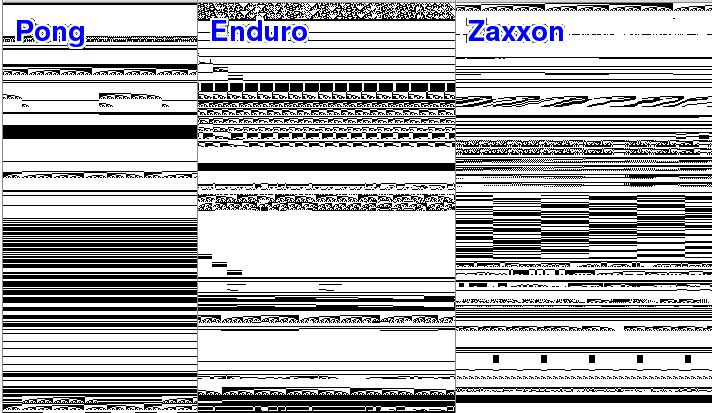
Motivated by very early infant development, we assume an unsupervised setup where our machine experiences a continuous stream of data, but has no external supervision or reward signals, and no actions to affect the environment. The machine receives a continuous stream of fixed-width vectors. In our experiments we use the sequence of 1024-bit memory states from Atari games concatenated with an 18-bit one-hot encoding of the previous action. We use the implementation available from OpenAI Gym [5]. An example of this data is shown in Figure 1 in the Supplementary Material. Since our system has no control, it’s merely watching another (random) player play games. Although our stream comes from multiple runs from different Atari games, the machine is given no special signal marking the beginning of an episode, nor is it given explicit information about which game is being played at any time. Though the machine’s goal is merely to remember and compress these sequences, we hypothesize that, in doing so, the machine will develop a model of the games that will be useful for a later time when it is given a reward signal.

In this setup, we want our system to be capable of learning new games indefinitely without forgetting earlier games. We would also like the system to leverage knowledge from earlier games to learn faster on new games.

We assume our vector memory works on floating-point vectors of a fixed size (we somewhat arbitrarily chose 64 elements for our implementations). We now discuss how such a memory can be used to store a virtually unlimited amount of sequential trace data.

Inspired by Complementary Learning Systems [24], we assume we have a large, though fixed, memory buffer (separate from the extendable vector memory) in which we can rotely store a long sequence of vectors. Our initial approach for compressing the data in this buffer was to train an LSTM Sequence to Sequence auto-encoder [31] to encode subsequences from this longer sequence (we used subsequences of length 7), then commit the 64-element-wide thought vectors for the subsequences to the vector-memory. There are several problems with this approach. One is that the amount of semantic knowledge is bounded by the weights of the LSTM auto-encoder. This means that we cannot expect the LSTM to keep learning the dynamics of new Atari games indefinitely.

To get around this, the number of free parameters for the LSTM models needs to be increased. One possibility was to simply increasing the number of hidden states in the LSTM, but each expansion would require us to address how to train the grown LSTM without causing catastrophic interference.

Our next approach was to train multiple LSTM auto-encoders, where each auto-encoder attempted to compress the input then reported a loss based on the difference between the original and decoded sequences. For each sequence, we tied together the losses with a minimum operation, which had the effect of only training the model that best encoded the sequence. In our experiments, this caused the models to specialize: When we trained three models on data from three different Atari games, each model specialized on encoding a particular game. (Of course, a single large LSTM with the same number of parameters has a lower reconstruction error than three small LSTMs, but the latter approach has the advantage of a simple straightforward way to extend the capacity of the model without risking catastrophic interference.)

One issue with using multiple LSTM auto-encoders is that our model’s semantic knowledge is stored outside the vector memory (i.e., in the weights of the LSTM auto-encoders). Since each model has 651,154 parameters, this is far too big to fit into a single vector of our vector memory (which we chose to store vectors of 64 elements). To address this, we reduced the dimensionality of the auto-encoders in a manner reminiscent of HyperNetworks [16] and learnets [3]. We trained 64-element embedding vectors for each LSTM by using a feedforward “stretcher” network shown in Figure 2a in the Supplementary Material, that “stretches” a vector of size 64 to size 651,154 using layers of 64, 128, 256, and 651,154 nodes. The final weights of the stretcher network are “reshaped” into the weights for an 64-hidden-unit LSTM auto-encoder. All the layers of the stretcher network are fully connected except the last layer, which is sparsely connected with only 1% of the possible connections, chosen randomly (a fully connected matrix would be too big to easily train). Thus, the parameter specification of each LSTM auto-encoder is a differentiable function of its 64-element embedding and the weights of the stretcher network, and thus backpropagation adjusts the embedding and the weights of the stretcher network instead of directly changing the auto-encoder’s parameters.

We dub the final embedding for each LSTM auto-encoder a ‘‘program vector’’, with the analogy that this embedding can be interpreted as a program that can be ‘‘called’’ with different thought-vectors or ‘‘arguments’’ to produce specific sequences. Of course, knowledge is stored in the weights of the stretcher network, which has a fixed number of parameters. We hope that the stretcher network becomes somewhat generic, only encoding very general knowledge after training on a wide variety of games⁴⁴ 4 Alternatively, one can imagine using a meta-stretcher network that allows us to embed many different stretcher networks, which could add another level of generality. At some point, there will have to be a fixed controller..

We hypothesize that the set of practically useful LSTM auto-encoders is only a tiny fraction of the set of those possible, and that the stretcher network will learn to generate “sensible” LSTMs with most 64-element vectors chosen from a 0, 1, Gaussian distribution.

We trained the stretcher network by training on sequences from various Atari games and varying the number of program vectors the system is allowed to use. The strongest result we have so far is that when the number of program vectors is equal to the number of Atari games, the system tends to use the same program vector for the same domain. That is, to some extent, it automatically segments the domains without being given explicit information which Atari game the traces are coming from. (See Figure 3 in the Supplementary Material).

Many expandable architectures have been proposed both recently and several decades ago. Non-parametric methods, such as Case-based reasoning [1], K-means and others (see [18] for a survey), have the ability to grow their capacity linearly with the data. Most of these methods operate on static vector data, so must be adapted to operate on sequential data. Furthermore, semantic knowledge (i.e., knowledge of patterns) is usually stored only implicitly (i.e., in the data points), unlike our proposed system which stores both instances and embeddings of semantic knowledge.

Other methods have been proposed to address catastrophic interference. For example, Complementary Learning Systems [24] and Learning without Forgetting [22] both interleave training of remembered earlier data with new data. We draw inspiration from both of these systems, and from work on Progressive Networks [27], which freezes weights of networks trained on earlier domains. Unlike the others, Progressive Networks allow a network to expand its capacity. Unlike our system, Progressive Networks do not attempt to store the semantic knowledge of earlier systems in a content addressable memory, and have the problem that their network grows quadratically in the number of domains. We hypothesize that storing semantic knowledge in a content addressable memory will help address this by allowing fast lookup of relevant “program vectors” potentially yielding linear storage and logarithmic program lookup.

Several methods have been proposed for expanding the capacity of neural networks. Part of our work was initially inspired by the Cascade Correlation algorithm [11], an early example which incrementally learns new features and adds them to a feed-forward network while freezing weights for previously learned features. Other models have since built on these ideas such as growing neural gas [12], Net2Net [6], and AdaNet [8]. Our work attempts to build on these ideas by providing a means of storing sequential instances in addition to semantic (weight) information.

There have been recent advances in differentiable memory, such as Neural Turing Machines [13], Memory Networks [35, 21], Differentiable Neural Computers [14], and Memory-based Deep Reinforcement Learning [23]. All of these provide the system with what is essentially a working memory that can be accessed during the course of a single episode. Unlike our system, the memory is cleared between episodes, so the only long-term memory these systems retain is in the network weights.

Episodic memory has also been a component of many cognitive architectures, such as SOAR [9], LIDA [26], and CLARION [30]. Our work was originally influenced specifically by SOAR [9], but extends these by using recent developments in sequence to sequence models to encode sequences as static vectors. Episodic memory has been shown to be useful for Reinforcement Learning tasks [4]. Our system provides a mechanism by which episodes may be stored and retrieved.

The primary contribution of our work is a system for encoding an unbounded amount of episodic and semantic knowledge in a expandable content-addressable vector memory. This work is still in its infancy and there are many unresolved issues to answer the question of how a machine can store a lifetime of knowledge such that it can be usefully retrieved and transferred to new situations. We share our current approaches for addressing some of these problems in the Supplementary Material.

Below, we provide a sample of the shortcomings of the current approach and what we are doing to address them.

References

- [1] David W Aha, Dennis Kibler, and Marc K Albert, Instance-based learning algorithms, Machine learning 6 (1991), no. 1, 37–66.
- [2] Thomas M Bartol Jr, Cailey Bromer, Justin Kinney, Michael A Chirillo, Jennifer N Bourne, Kristen M Harris, and Terrence J Sejnowski, Nanoconnectomic upper bound on the variability of synaptic plasticity, Elife 4 (2015), e10778.
- [3] Luca Bertinetto, João F. Henriques, Jack Valmadre, Philip H. S. Torr, and Andrea Vedaldi, Learning feed-forward one-shot learners, CoRR abs/1606.05233 (2016).
- [4] Charles Blundell, Benigno Uria, Alexander Pritzel, Yazhe Li, Avraham Ruderman, Joel Z Leibo, Jack Rae, Daan Wierstra, and Demis Hassabis, Model-free episodic control, arXiv preprint arXiv:1606.04460 (2016).
- [5] Greg Brockman, Vicki Cheung, Ludwig Pettersson, Jonas Schneider, John Schulman, Jie Tang, and Wojciech Zaremba, Openai gym, 2016.
- [6] Tianqi Chen, Ian Goodfellow, and Jonathon Shlens, Net2net: Accelerating learning via knowledge transfer, arXiv preprint arXiv:1511.05641 (2015).
- [7] Junyoung Chung, Sungjin Ahn, and Yoshua Bengio, Hierarchical multiscale recurrent neural networks, arXiv preprint arXiv:1609.01704 (2016).
- [8] Corinna Cortes, Xavi Gonzalvo, Vitaly Kuznetsov, Mehryar Mohri, and Scott Yang, Adanet: Adaptive structural learning of artificial neural networks, arXiv preprint arXiv:1607.01097 (2016).
- [9] Nate Derbinsky and John E Laird, Efficiently implementing episodic memory, International Conference on Case-Based Reasoning, Springer, 2009, pp. 403–417.
- [10] David A Drachman, Do we have brain to spare?, Neurology 64 (2005), no. 12, 2004–2005.
- [11] Scott E Fahlman and Christian Lebiere, The cascade-correlation learning architecture, (1989).
- [12] Bernd Fritzke et al., A growing neural gas network learns topologies, Advances in neural information processing systems 7 (1995), 625–632.
- [13] Alex Graves, Greg Wayne, and Ivo Danihelka, Neural turing machines, arXiv preprint arXiv:1410.5401 (2014).
- [14] Alex Graves, Greg Wayne, Malcolm Reynolds, Tim Harley, Ivo Danihelka, Agnieszka Grabska-Barwińska, Sergio Gómez Colmenarejo, Edward Grefenstette, Tiago Ramalho, John Agapiou, Adrià Puigdomènech Badia, Karl Moritz Hermann, Yori Zwols, Georg Ostrovski, Adam Cain, Helen King, Christopher Summerfield, Phil Blunsom, Koray Kavukcuoglu, and Demis Hassabis, Hybrid computing using a neural network with dynamic external memory, Nature (2016).
- [15] Karol Gregor, Ivo Danihelka, Alex Graves, Danilo Jimenez Rezende, and Daan Wierstra, Draw: A recurrent neural network for image generation, arXiv preprint arXiv:1502.04623 (2015).
- [16] David Ha, Andrew Dai, and Quoc V Le, Hypernetworks, arXiv preprint arXiv:1609.09106 (2016).
- [17] Kaiming He, Xiangyu Zhang, Shaoqing Ren, and Jian Sun, Deep residual learning for image recognition, arXiv preprint arXiv:1512.03385 (2015).
- [18] Myles Hollander, Douglas A Wolfe, and Eric Chicken, Nonparametric statistical methods, John Wiley & Sons, 2013.
- [19] Pentti Kanerva, Sparse Distributed Memory, MIT Press, Cambridge, MA, USA, 1988.
- [20] Ryan Kiros, Yukun Zhu, Ruslan R Salakhutdinov, Richard Zemel, Raquel Urtasun, Antonio Torralba, and Sanja Fidler, Skip-thought vectors, Advances in neural information processing systems, 2015, pp. 3294–3302.
- [21] Ankit Kumar, Ozan Irsoy, Jonathan Su, James Bradbury, Robert English, Brian Pierce, Peter Ondruska, Ishaan Gulrajani, and Richard Socher, Ask me anything: Dynamic memory networks for natural language processing, arXiv preprint arXiv:1506.07285 (2015).
- [22] Zhizhong Li and Derek Hoiem, Learning without forgetting, European Conference on Computer Vision, Springer, 2016, pp. 614–629.
- [23] Junhyuk Oh, Valliappa Chockalingam, Satinder Singh, and Honglak Lee, Control of memory, active perception, and action in minecraft, arXiv preprint arXiv:1605.09128 (2016).
- [24] Randall C O’Reilly, Rajan Bhattacharyya, Michael D Howard, and Nicholas Ketz, Complementary learning systems, Cognitive Science 38 (2014), no. 6, 1229–1248.
- [25] Bente Pakkenberg and Hans Jørgen G Gundersen, Neocortical neuron number in humans: effect of sex and age, Journal of Comparative Neurology 384 (1997), no. 2, 312–320.
- [26] Uma Ramamurthy and Stan Franklin, Memory systems for cognitive agents, Proceedings of Human Memory for Artificial Agents Symposium at the Artificial Intelligence and Simulation of Behavior Convention (AISB’11), 2011, pp. 35–40.
- [27] Andrei A Rusu, Neil C Rabinowitz, Guillaume Desjardins, Hubert Soyer, James Kirkpatrick, Koray Kavukcuoglu, Razvan Pascanu, and Raia Hadsell, Progressive neural networks, arXiv preprint arXiv:1606.04671 (2016).
- [28] Juergen Schmidhuber, On learning to think: Algorithmic information theory for novel combinations of reinforcement learning controllers and recurrent neural world models, arXiv preprint arXiv:1511.09249 (2015).
- [29] Terrence C Stewart, Yichuan Tang, and Chris Eliasmith, A biologically realistic cleanup memory: Autoassociation in spiking neurons, Cognitive Systems Research 12 (2011), no. 2, 84–92.
- [30] Ron Sun, Memory systems within a cognitive architecture, New Ideas in Psychology 30 (2012), no. 2, 227–240.
- [31] Ilya Sutskever, Oriol Vinyals, and Quoc V Le, Sequence to sequence learning with neural networks, Advances in neural information processing systems, 2014, pp. 3104–3112.
- [32] Andrew Trask, David Gilmore, and Matthew Russell, Modeling order in neural word embeddings at scale, Proceedings of the 32nd International Conference on Machine Learning (ICML), 2015, pp. 2266–2275.
- [33] Endel Tulving, What is episodic memory?, Current Directions in Psychological Science 2 (1993), no. 3, 67–70.
- [34] Jingdong Wang, Heng Tao Shen, Jingkuan Song, and Jianqiu Ji, Hashing for similarity search: A survey, arXiv preprint arXiv:1408.2927 (2014).
- [35] Jason Weston, Sumit Chopra, and Antoine Bordes, Memory networks, arXiv preprint arXiv:1410.3916 (2014).
Supplementary Material
7 Approaches for Addressing Shortcomings of the Current Approach