The Spread of Cooperative Strategies on Grids with Random Asynchronous Updating

The particular topology of a network has a dramatic impact on discrete processes that model competitive interactions in communities [11]. For example, spread of a particular attitude or belief is less likely to propagate completely in Erdös-Renyi graphs than on small-world networks [4]. Studies of Cellular Automata indicate that the particular updating scheme impacts the limiting configuration of randomly seeded cellular automaton [15]. Here we combine these two paradigms to study a discrete-time process that may be modelled as a cellular automata with a particular updating scheme.

The Prisoner’s Dilemma, a staple of classical game theory, is a $2$-player game in which each of the two players simultaneously make a decision to either cooperate or defect. Each of the players receives a pay-off whose amount takes into account the decisions of both players. The pay-off structure is chosen so that each player’s pay-off is maximised when both choose cooperate and so that a player’s pay-off is minimized when they choose cooperate and the other player chooses to defect. Classically the game is played in a single round. However by considering the game as being played in a series of rounds, the Prisoner’s Dilemma may be used to model a variety of scenarios in many disciplines, including evolutionary biology [18, 7], economics [19, 9] and sociology [10, 17]. More broadly, the Prisoner’s Dilemma on graphs fits in the context of evolutionary games on graphs. A survey of methods and research in this area is given in [20].

Here we consider the iterated Prisoner’s Dilemma as a game played between neighbours on a graph. In each round each vertex plays, with a fixed strategy (cooperate or defect), the game with each of its neighbours. The score for each vertex is the sum of the pay-offs its receives in each game. At the end of each round, each vertex is given the opportunity to update their strategy to that of their most successful neighbour.

The Prisoner’s Dilemma on the grid was first examined by Nowak and May [12]. Through simulation they find that spatial effects have an impact on the evolution of the strategies of players in the process. In examining symmetric configurations they find “dynamical fractals” and “evolutionary kaleidoscopes”. In this early work, the authors consider an update scheme in which each of the vertices update simultaneously to emulate the strategy of their most successful neighbour. This updating scheme has been examined on a variety of different graphs, in particular regular lattices, random graphs and small-world networks. For example, Abramson and Kuperman observe a number of properties of a Prisoner’s Dilemma process for regular lattices and random graphs [2]; Durán and Mulet observe a relationship between initial and final density of cooperators on random graphs when the graph has small connectivity [8]; Santos et al. consider how the preferential model of attachment in random graphs provide sufficient conditions for the cooperator strategy to propagate [14].

In much of the previous work in this area, the authors consider a deterministic model of updating in which all of the vertices simultaneously emulate the strategy of their most successful neighbour. However, other update schemes are possible. In [21] the authors use a probabilistic process as part of the updating strategies. In addition to synchronous updating schemes, i.e., those in which all vertices update simultaneously, asynchronous schemes may be studied. In their survey of evolutionary games on graphs [20], Szabó and Fáth consider the update model in which a pair of neighbouring vertices are chosen at random, with one emulating the strategy of the other according to some random variable.

A study of asynchronous update schemes of cellular automata by Cornforth et al. shows that the particular variant of asynchronous update has a dramatic effect on the limiting behaviour of one dimensional cellular automata [5]. They further highlight the differences between deterministic and probabilistic asynchronous update schemes. A full survey of asynchronous update schemes in cellular automata is given in [6]. The model of asynchronous probabilistic updating presented here provides a new direction in both the study of cellular automata and evolutionary games on graphs. We propose a variation of the random independent model of updating that considers the set of vertices envious of their neighbours and updates them in a random order, playing a round of the game after each individual vertex has updated. This update scheme behaves similarly to the random independent model for updating cellular automata [15]; however, it provides necessary structure to facilitate proofs of observed behaviours.

We note that in many of these previous works, much of the work has been strictly experimental. That is, emergent behaviours are observed through carefully designed computer simulation. A notable exception to this is the work of Schweitzer et al. [16], whose analysis allows for a verification of the simulations originally presented by Nowak and May. Here we break from this trend to provide theoretical justifications for observed behaviours.

In this paper we study the resulting behaviour of the Prisoner’s Dilemma process on toroidal grids where each vertex of the grid cooperates with probability $p\in[0,1]$. Figure 2 gives examples of starting and the resulting stable configurations for various values of $p$. Here we notice that, though the initial configuration is randomised, the resulting stable configuration exhibits a surprising amount of structure. While the update process introduces uncertainty through the choice of the permutation of the envious vertices, we find that for some values of $p$, we may predict the density of cooperators as $t\to\infty$. In Section 3 we consider the growth of small clusters existing in infinite grids. We use the results from Section 3 in Section 4 to derive probabilistic bounds on the final density of cooperators on the $n\times n$ toroidal grid for a fixed value of $p$, and for $p$ as a function of $n$.

Let $G=(V,E)$ be a graph. A configuration, $C$, is a function that assigns a strategy to each vertex of $G$. Formally, $C:V\rightarrow\{0,1\}$, where $0$ corresponds to defector and $1$ corresponds to cooperator. The pay-off function, $f$, assigns the score for the first player to an ordered pair that represents the strategies of the first and second player. The pay-off function $f:\{0,1\}\times\{0,1\}\rightarrow\{0,1,T\}$ is given by

where $T>1$ is a fixed constant. We refer to $T$ as the cheating advantage.

Let $C$ be fixed and let $v\in V(G)$. The score of $v$ with respect to $C$ is given by

When the context is clear we refer to the score of $v$. The most successful neighbours of $v$ are the vertices in the closed neighbourhood of $v$ (denoted $N[v]$) that have the greatest score. We restrict our consideration for possibilities for the value $T$ in such a way that each of the most successful neighbours have the same strategy. Let $u$ be a most successful neighbour of $v$. The vertex $v$ is called weak with respect to $C$ if $C(v)\neq C(u)$. Otherwise, we say that $v$ is strong. In other words, weak vertices would like to change their strategy and strong vertices are satisfied with their strategy. We are interested in the change in the configuration with respect to time; we use $C_{t}$ to denote the configuration at time $t$ and $s_{t}$ to denote the score at time $t$.

The configuration, $D$, resulting from updating $v$ with respect to $C$ changes the strategy of $v$ if $v$ is weak and leaves the strategies of all other vertices fixed.

We call a maximal connected proper subgraph $K$ of $k$ vertices with the same strategy a $k$-cluster. We say that a $1$-cluster is an isolated vertex. The $k$-cluster $H\leq G$ has a border of width $b$ if for all $h\in V(H)$ and all $v\in V(G-H)$ such that $C(h)=C(v)$, we have that $d(h,v)\geq b$. That is, $H$ is surrounded by a border that $b$ vertices wide that consists of vertices all with the opposite strategy.

Given a graph $G$ and some $T>1$, our process is initialised with $C_{0}$, some configuration of the vertices. The process proceeds as follows. Let $W_{t}$ be the set of weak vertices with respect to $C_{t}$. If $W_{t}=\emptyset$, then the process terminates. In this case we say that $C_{t}$ is a stable configuration. Otherwise, we select with uniform probability a permutation, $\sigma$, of the elements of $W_{t}$. Considering the permutation as a sequence of the elements of $W_{t}$, we proceed through $|W_{t}|$ subrounds. At the $k^{th}$ subround we update the $k^{th}$ vertex of the sequence, $v_{k}$, with respect to the current configuration (i.e., the configuration resulting from the $(k-1)^{th}$ subround). The configuration resulting from the $|W_{t}|^{th}$ subround is denoted $C_{t+1}$. We refer to the process as the Prisoner’s Dilemma process on $G$ with randomised asynchronous updating. Though, for brevity we refer to this process as the PD process on $G$.

Let $C$ be a configuration and $\sigma$ a permutation of the elements of $W$. For any vertex $x\in W$ we denote by $\sigma^{-1}(x)$ the position of $x$ in the sequence of elements of $W$ induced by $\sigma$. Thus, $x$ is updated in the $\sigma^{-1}(x)$ subround.

As we are interested in the spread of the cooperative strategy, for any configuration we may consider the density of cooperators. For configuration $C_{t}$, let $r_{t}$ be the density of cooperators at time $t$. If $C_{t}$ is a stable configuration, then we define the final density, denoted $r_{f}$, to be $r_{t}$.

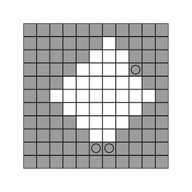
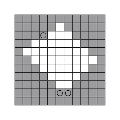
We give an example on the $6\times 6$ grid to highlight how the choice of $T$ for the process and the choice of the updating permutation in a particular round affect the spread of strategies. Consider the configuration given in Figure 1(a). In our figures we use white squares for cooperators and grey squares for defectors.

If $T=\frac{5}{3}$ each of the cooperators have score $2$ and each of the labelled defectors have score $\frac{5}{3}$. All unlabelled vertices have score $0$, as they are defectors with no cooperator neighbours. Observe that $W_{0}=\{v_{1},v_{2},\dots,v_{8}\}$. Figure 1(b) gives the resulting configurations after applying $\sigma_{1}=(v_{2},v_{3},v_{6},v_{7},v_{1},v_{4},v_{5},v_{8})$ to $C_{0}$ and alternatively applying $\sigma_{2}=(v_{2},v_{4},v_{6},v_{8},v_{1},v_{3},v_{5},v_{7})$ to $C_{0}$. In the first case, after subround $4$, $v_{1}$ is no longer a weak vertex, and so does not change strategy. The configuration $C_{1}$ has no weak vertices and thus is stable. However, in the second case, $v_{1}$ is a weak vertex after subround $4$, and so does change from being a cooperator to a defector. In this second case, the resulting configuration has eight weak vertices.

For $T=\frac{8}{3}$, each of the cooperators have score $2$, and each of the labelled defectors have score $\frac{8}{3}$. All unlabelled vertices have score $0$, as they are defectors with no cooperator neighbours. Observe that $W_{0}=\{u_{1},u_{2},u_{3},u_{4}\}$. Regardless of the choice $\sigma$, Figure 1(c) is the resulting configuration after round $0$.

A configuration $C_{t}$ is called forced if $C_{t+1}$ will be the configuration regardless of the choice of $\sigma$ at time $t$. For a sequence $C_{0},C_{1},\dots$ of configurations, we call the sequence resulting from removing the forced configurations, and re-indexing, the basic sequence. We use the notation $C_{0}^{\prime},C_{1}^{\prime},\dots$ to refer to a basic sequence and use the term basic time steps to refer to the time steps in a basic sequence.

In a $4$-regular graph, if $1<T<\frac{4}{3}$, then the most successful neighbour of $v$ is the vertex in the closed neighbourhood of $v$ with the most cooperator neighbours, with defectors taking precedence in the case of a draw. For the remainder of this paper we consider only the case $1<T<\frac{4}{3}$ as we restrict our study to the toroidal grid. We use the notation $T=1+\epsilon$ to refer to $T$ in this range and use $k+\epsilon$ to refer to a score between $k$ and $k+1$. Thus, we say that a defector with $k$ cooperator neighbours has score $k+\epsilon$.

In this section we consider the evolution of clusters situated in infinite grids. We apply these results in Section 4 to study the behaviour of $r_{t}$ in the $n\times n$ toroidal grid.

Up to rotation and reflection of the plane, there is a single $1$-cluster of defectors and a single $2$-cluster of defectors. A configuration of a single defector in an infinite grid of cooperators has exactly four weak vertices – the neighbours of the single defector. By examining the number of cooperator neighbours, we see that when one of these weak vertices has become a cooperator the resulting configuration is stable. Therefore a $1$-cluster of defectors in an infinite field of cooperators evolves to a $2$-cluster of defectors, which is a stable configuration. To show that the spread of a $k$-cluster of defectors in an infinite grid of cooperators is bounded, we require the following results.

For a configuration $C_{i}$, we say that a cooperator $v$ is a persistent cooperator if $C_{t}(v)=1$ for all $t\geq i$.

In this case we say that $v$ is a initial persistent cooperator

Together these results allow us to find a bound on the growth of a $k$-cluster of defectors in an infinite field of cooperators.

As we consider the evolution of $k$-clusters of cooperators in an infinite field of defectors we encounter some cases for which there are no surviving cooperators. In this case, we say that the particular cluster evolves to an empty cluster.

Up to symmetry of the plane, there is a single $1$-cluster and a single $2$-cluster. When placed in a sufficiently large grid of defectors, each of these clusters evolves to an empty cluster after at most two time steps.

Up to rotation and reflection there are two species of $3$-clusters: $3$-lines and $3$-corners. When placed in a sufficiently large field of defectors, a $3$-line evolves to a stable configuration containing a $5$-cluster with probability $1$. A $3$-corner evolves to a stable configuration containing a $5$-cluster with probability $\frac{1}{2}$ and to an empty cluster with probability $\frac{1}{2}$. The evolution of these clusters is given in Figure 3(a). Note that weak vertices are indicated with a circle.

Up to rotation and reflection there are $5$ species of $4$-clusters: $4$-lines, $4$-corners, $4$-hats, $4$-turns, and $4$-squares (See Figure 3). A $4$-hat stabilises to a stable $5$-cluster with probability $1$. However, for each of the other configurations simulation suggests a non-zero probability of large growth. The evolution of these clusters through a small number of iterations is given in Figure 3.

We wish to show that a $4$-cluster in an infinite grid of defectors will eventually evolve to a stable configuration. Though the growth of such clusters passes through many different configurations, we show that every configuration in the sequence of basic configurations where $C_{0}$ is a $4$-cluster of cooperators in an infinite field of defectors can be classified into one of eight types. We consider these types equivalent under rotation and reflection. The width parameter of each type tells the number of columns that contain cooperators, whereas the height parameter tells us how many cooperators are in the column with the greatest amount of cooperators. A summary of the configurations is given in Table 1. We note that each of these configurations is convex. That is, for any pair of cooperators contained in a cluster, there is a shortest path between them that contains only cooperators.

We begin by defining four basic clusters, which take the form of skew rectangles.

The stable cluster of width $w\geq 3$ and height $h\geq 3$ $(h\equiv 1\bmod 2,w-h\geq 0)$ consists of cooperators in $w$ columns. The first column (starting from the left) contains a single cooperator. The number of cooperators increases by $2$ in each subsequent column, until a column of height $h$ is reached. These increasing columns are aligned so that the previous column is vertically centred in the subsequent column. After the maximum is reached, columns of height $h$ repeat $w-h\geq 0$ times so that there are $w$ columns containing cooperators, as shown in Figure 4(a). These repeating columns of height $h$ are offset in such a way so that a subsequent column is one unit lower than the previous column Following these repeating columns are columns whose heights decrease by $2$ in each subsequent column until there is a column with a single cooperator. An example is given in Figure 4(a). Observe that such a configuration is stable when placed in an infinite field of defectors. We use the symbol $\includegraphics[width=10.00002pt]{Figures/glyphs/stableNEW.pdf}_{w,h}$ to denote a stable cluster of width $w$ and height $h$.

The doubly even cluster of height $h\geq 2$ and width $w\geq 2$ $(h\equiv 1\bmod 2,w-h+1\geq 0)$ is a cluster consisting of cooperators in $w$ columns. The first column (starting from the left) contains two cooperators. The number of cooperators increase by $2$ in each subsequent column, until a column of height $h-1$ is reached. These increasing columns are aligned so that the previous column is vertically centred in the subsequent column. If $w-h+1=0$, then there a second column of height $h-1$ aligned with the first column of height $h-1$. The heights of the columns then decrease by $2$ in each subsequent column until there is a column with a single cooperator. Otherwise if $w-h+1>0$, then the column of height $h-1$ is followed by $w-h+1$ columns of height $h$. The first of these columns is aligned so that the top of this column aligns with the column of height $h-1$. Subsequent columns of height $h$ are offset so a subsequent column is one unit lower than the previous column. Following these repeating columns is a column of height $h$ there is a column of height $h-1$. This column of height $h-1$ is aligned so the bottom of this column is aligned with that of the previous column. The heights of the columns then decrease by $2$ in each subsequent column until there is a column with a two cooperators. An example is given in Figure 4(b). We use the symbol $\includegraphics[width=10.00002pt]{Figures/glyphs/4flatNEW.pdf}_{w,h}$ to denote the doubly even cluster of height $h$ and width $w$. Observe that $\includegraphics[width=10.00002pt]{Figures/glyphs/4flatNEW.pdf}_{w,h}$ has $8$ weak vertices when placed in an infinite field of defectors.

The opposite even cluster of height $h\geq 3$ and width $w\geq 4$ $(h\equiv 0\bmod 2,w-h\geq 0)$ is a cluster of cooperators in $w$ columns. The first column (starting from the left) contains one cooperator. The number of cooperators increases by $2$ in each subsequent column, until $h-1$ is reached. These increasing columns are aligned so that the previous column is vertically centred in the subsequent column. If $w-h=0$, then the column of height $h-1$ is followed by a second column of height $h-1$. This second column of height $h-1$ is aligned with the previous column of height $h-1$. The heights of the columns then decrease by $2$ in each subsequent column until there is a column with a single cooperator. Otherwise if $w-h>0$, then the column of height $h-1$ is followed $w-h$ columns of height $h$. The first of these is aligned so that the top of this column is aligned with the top of the previous column of height $h-1$. Subsequent columns of height $h$ are offset so a subsequent column is are one unit lower than the previous column. These columns of height $h$ are followed by a column of height $h-1$. This column of height $h-1$ is aligned with the bottom of the previous column of height $h$. The heights of the columns then decrease by $2$ in each subsequent column until there is a column with a single cooperator. An example is given in Figure 4(c). We use the symbol $\includegraphics[width=10.00002pt]{Figures/glyphs/2flatoppNEW.pdf}_{w,h}$ to denote the opposite even cluster of height $h$ and width $w$. Observe that $\includegraphics[width=10.00002pt]{Figures/glyphs/2flatoppNEW.pdf}_{w,h}$ has four weak vertices when placed in an infinite field of defectors.

The adjacent even cluster of height $h\geq 5$ and width $w\geq 5$ $(h\equiv 0\bmod 2)$ is a cluster of cooperators in $w$ columns. The first column (starting from the left) contains two cooperators. The number of cooperators increases by $2$ in each subsequent column, until a column of height $h$ is reached. These increasing columns are aligned so that so that the previous column is vertically centred in the subsequent column. These increasing columns are followed by $w-h$ columns of height $h$ so that there are $w$ columns containing cooperators, as shown in Figure 4(d) . These repeating columns of height $h$ are offset so that a subsequent column is are one unit lower than the previous column. The repeating columns of height $h$ are followed by a column of height $h-1$. This bottom of the column of height $h-1$ is aligned with the bottom of the final column of height $h$. The heights of the columns then decrease by $2$ in each subsequent column until there is a column with a single cooperator. An example is given in Figure 4(d). We use the symbol $\includegraphics[width=10.00002pt]{Figures/glyphs/2flatadjNEW.pdf}_{w,h}$ to denote the adjacent even cluster of height $h$ and width $w$. Observe that $\includegraphics[width=10.00002pt]{Figures/glyphs/2flatadjNEW.pdf}_{w,h}$ has four weak vertices when placed in an infinite field of defectors.

From these last two skew rectangular clusters, we define four transit clusters. These four transit clusters arise by considering the evolution of the skew rectangular clusters placed in an infinite field of defectors. Consider the cluster given in Figure 4(d). We see a pair of weak vertices aligned vertically on the left side of the figure and a pair of weak vertices aligned horizontally at the bottom of the figure. In the subsequent round exactly one defector from each pair will turn to a collaborator. Assume that the upper weak vertex on the left side of the figure and the left vertex on the bottom of the figure turn to collaborators in the following round. In this case we see that the next three time-steps are forced, as the $NW$ and $SW$ side of the cluster grow. Since the $NW$ side is shorter than the $SW$ side, when the next basic time-step is reached the $SW$ side has not yet been fully filled in. We can consider such a cluster as being formed from a copy by adding some number of collaborators along one of the sides. In a similar way, we can also construct a cluster from a copy of by adding collaborators along one of the sides.

The double even transit cluster of width $w$, height $h$ and length $\ell$ ($1\leq\ell<\frac{h}{2}$) is formed in two ways based on the value of $\ell$. To describe this cluster, we must consider $\includegraphics[width=10.00002pt]{Figures/glyphs/2flatoppNEW.pdf}_{w,h}$ placed in an infinite field of defectors. Such a cluster has two pairs of weak vertices – those at the top of the cluster and those at the bottom of the cluster. When $\ell=1$ the double even transit cluster of width $w$, height $h$ and length $\ell=1$ is formed by changing the upper-right weak defector to a collaborator. We note that the double even transit cluster of width $w$, height $h$ and length $\ell=1$ has three weak vertices when placed in an infinite field of defectors. One of these weak vertices, say $x$, has no weak neighbours. When $1<\ell<\frac{h}{2}$ we define this cluster inductively. The double even transit cluster of width $w$, height $h$ and length $1<\ell<\frac{h}{2}$ is formed from the the double even transit cluster of width $w$, height $h$ and length $\ell-1$ by changing $x$ to be a cooperator. We note that the double even transit cluster of width $w$, height $h$ and length $1\leq\ell<\frac{h}{2}$ has three weak vertices when placed in an infinite field of defectors. One of these weak vertices, say $x$, has no weak neighbours. We use the symbol $\includegraphics[width=10.00002pt]{Figures/glyphs/1flatopp2NEW.pdf}_{w,h,\ell}$ to denote the double even transit cluster of width $w$, height $h$ and length $\ell$.

The following two transit clusters are formed from . Consider $\includegraphics[width=10.00002pt]{Figures/glyphs/2flatadjNEW.pdf}_{w,h}$ placed in an infinite field of defectors. Such a cluster has two pairs of weak vertices – those at the left of the cluster and those at the bottom of the cluster. The two following clusters arise by adding, respectively, collaborators along the $NW$ side and along the $SW$ side starting from the left side of the cluster.

The adjacent even transit cluster of width $w$, height $h$ and length $\ell$ of type A (resp. type B) ($1\leq\ell<h/2$) is formed in two ways based on the value of $\ell$. When $\ell=1$, the adjacent even transit cluster of width $w$, height $h$ and length $\ell=1$ of type A (resp. type B) is formed from $\includegraphics[width=10.00002pt]{Figures/glyphs/2flatadjNEW.pdf}_{w,h}$ by changing the lower (resp. upper) of the two weak vertices on the left side of the cluster to be collaborators. Observe that such a cluster has three weak vertices. One of these weak vertices, say $x$, has no weak neighbours. For $1<\ell<\frac{h}{2}$ we define this cluster inductively. The adjacent even transit cluster of width $w$, height $h$ and length $1<\ell<\frac{h}{2}$ of type A (resp. type B) is formed from an adjacent even transit cluster of width $w$, height $h$ and length $\ell-1$ of type A (resp. type B) by changing $x$ to be a cooperator. We note that the adjacent even transit cluster of width $w$, height $h$ and length $1\leq\ell<\frac{h}{2}$ of type A (resp. type B) has three weak vertices when placed in an infinite field of defectors. One of these weak vertices, say $x$, has no weak neighbours. We use the symbol $\includegraphics[width=10.00002pt]{Figures/glyphs/1flatadj2NEW.pdf}_{w,h,\ell}$ (resp.$\includegraphics[width=10.00002pt]{Figures/glyphs/1flatopp1NEW.pdf}_{w,h,\ell}$) to denote the adjacent even transit cluster of width $w$, height $h$ and length $\ell$ of type A. See Figure 5(c) for an example.

Finally, we reach our ultimate transit cluster – the adjacent even transit cluster of width $w$, height $h$ and length $\ell$ of type C ($0\leq\ell<h/2$, $w,h\equiv 0\bmod 2)$. We describe this cluster using the same methodology as the basic clusters. This cluster consist of cooperators in $w$ columns. We begin with the case $\ell=0$. The first column (starting from the left) contains a single cooperator. The number of cooperators increases by $2$ in each subsequent column, until a column of height $h-4$ is reached. These increasing columns are aligned so that so that the previous column is vertically centred in the subsequent column. This column of height $h-3$ is followed by a column of height $h-1$. The column of height $h-3$ is aligned with that of height $h-1$ so that the bottom of the column of height $h-3$ is aligned with the vertex that is third from bottom in the column of height $h-1$. The column of height $h-1$ is followed by a column of height $h$. The bottom of the column of height $h-1$ is aligned with the bottom of the column of height $h$. The column of height $h$ is then followed by $w-h-3$ columns of height $h$. These repeating columns of height $h$ are aligned so that a subsequent column is one unit higher than a previous column. Following the repeating columns of height $h$ are columns whose heights decrease by $2$ until a column of height $1$ is reached. We note that adjacent even transit cluster of width $w$, height $h$ and length $\ell=0$ of type C has three weak vertices when placed in an infinite field of defectors. One of these vertices, say $x$, has no weak neighbours. For $1\leq\ell<\frac{h}{2}$ we define this cluster inductively. The adjacent even transit cluster of width $w$, height $h$ and length $1\leq\ell<\frac{h}{2}$ of type C is formed from the adjacent even transit cluster of width $w$, height $h$ and length $\ell-1$ of type C by changing $x$ to be a cooperator. We note that the adjacent even transit cluster of width $w$, height $h$ and length $1\leq\ell<\frac{h}{2}$ of type C has three weak vertices when placed in an infinite field of defectors. One of these weak vertices, say $x$, has no weak neighbours. We use the symbol $\includegraphics[width=10.00002pt]{Figures/glyphs/1flatadj1NEW.pdf}_{w,h,\ell}$ to denote the adjacent even transit cluster of width $w$, height $h$ and length $\ell$ of type C. See Figure 5(d) for an example.

Let $\mathcal{D}$ be the set of configurations listed above together with their reflections and rotations in the plane across all possible values of $w$, $h$ and $\ell$.

To show how transitions occur between elements of $\mathcal{D}$, consider the sequences of configurations given in Figure 6. Recall that elements of $\mathcal{D}$ are considered equivalent up to reflection and rotation. Examining $C_{0}$ we see that there are $4!$ updating permutations. Let $u_{1}$ and $u_{2}$ be the pair of horizontal weak vertices so that $u_{1}$ is to the left of $u_{2}$, and $v_{1}$ and $v_{2}$ be the pair of vertical weak vertices so that $v_{1}$ is above $v_{2}$. In considering the possible updating permutations we note that for each pair of adjacent weak vertices it only matters which of the pair comes first. That is, the sequence $u_{1},v_{1},u_{2},v_{2}$ will give the same resulting configuration as $u_{1},u_{2},v_{1},v_{2}$. By also considering the symmetries of the cluster, the $4!$ possible updating sequences may be partitioned in the three equivalence classes. Sequences $C$,$D$ and $E$ give the resulting sequence of configurations given by the equivalence classes with representative elements (permutations): $(u_{1},v_{1},u_{2},v_{2}),(u_{2},v_{1},u_{2},v_{1})$ and $(u_{2},v_{2},u_{1},v_{1})$, respectively. By analysing the equivalence classes, $C$ and $D$ each occur with probability $\frac{1}{4}$, and $E$ occurs with probability $\frac{1}{2}$. After proceeding through the forced iterations, we see that in each case we arrive at an element of $\mathcal{D}$. In particular, $\includegraphics[width=10.00002pt]{Figures/glyphs/2flatadjNEW.pdf}_{8,7}$ transitions to with probability $\frac{1}{4}$, to $\includegraphics[width=10.00002pt]{Figures/glyphs/2flatadjNEW.pdf}_{8,9}$ with probability $\frac{1}{4}$ and to $\includegraphics[width=10.00002pt]{Figures/glyphs/1flatadj1NEW.pdf}_{9,8,3}$ with probability $\frac{1}{2}$. We note that by a similar analysis for other elements of $\mathcal{D}$, if $C_{i}^{\prime}\in\mathcal{D}$, then $C_{i+1}^{\prime}\in\mathcal{D}$.

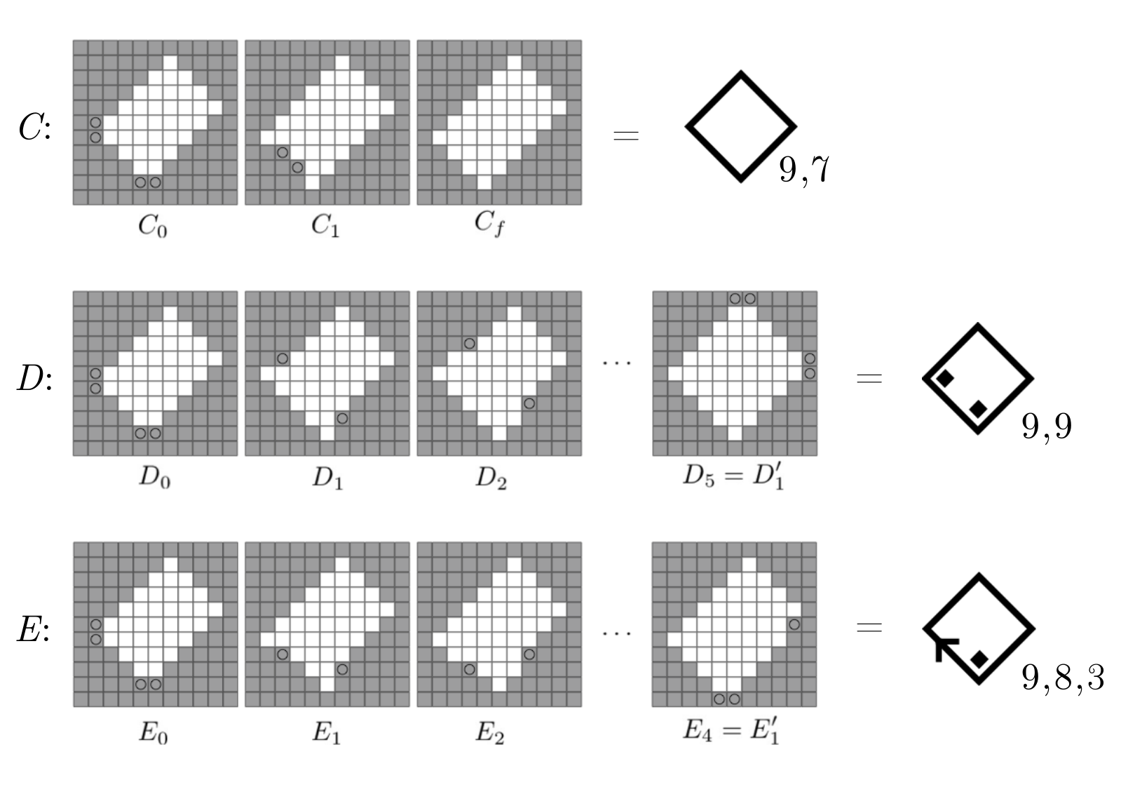
Figure 7 gives a partial transition diagram for the elements of $\mathcal{D}$. The transitions shown do not depend on the particular values of $w$ and $h$. For example, regardless of the values of $w$ and $h$, an element of $\mathcal{D}$ of the form $\includegraphics[width=10.00002pt]{Figures/glyphs/4flatNEW.pdf}_{w,h}$ will transition to $\includegraphics[width=10.00002pt]{Figures/glyphs/stableNEW.pdf}_{w+2,h+2}$ with probability $\frac{1}{8}$. However the transition of an element of the form $\includegraphics[width=10.00002pt]{Figures/glyphs/2flatadjNEW.pdf}_{w,h}$ will only transform to an element of the form $\includegraphics[width=10.00002pt]{Figures/glyphs/2flatadjNEW.pdf}_{w+1,h+1}$ (with probability $\frac{1}{4}$) if $w=h$. From this diagram we see that each element of $\mathcal{D}$ that is not a stable cluster can transition to a stable cluster after at most $3$ basic time-steps. Such a transition will occur with probability at least $\frac{1}{8}$. This fact is given by the following lemma.

Figure 7 is constructed to show that regardless of the configuration in $C_{i}^{\prime}$, it is possible that one of $C_{i+1}^{\prime},C_{i+2}^{\prime}$ or $C_{i+3}^{\prime}$ is . As such, there are transitions between elements of $\mathcal{D}$ that can be deduced, but are not shown in Figure 7. For example if $w=h$ then $\includegraphics[width=10.00002pt]{Figures/glyphs/2flatadjNEW.pdf}_{w,h}$ transitions to $\includegraphics[width=10.00002pt]{Figures/glyphs/2flatadjNEW.pdf}_{w+2,h+2}$ with probability $\frac{3}{4}$. This transition, and many others, are omitted from Figure 7 as they are not relevant to Lemma 5. As the omitted transitions are both cumbersome to enumerate and do not aid in the analysis below, we shall refrain from enumerating them.

Lemma 5 implies the following corollary about the termination of the PD process seeded with a $4$-cluster of cooperators in an infinite grid of defectors.

Corollary 7 allows us to provide a crude upper bound on the expected growth of a $4$-cluster of cooperators in an infinite field of defectors.

We note that, though the sum in Theorem 8 does converge, the value is much more than the actual growth of a $4$-cluster as observed in simulations. This bound may be improved by observing that in the first few configurations appears very frequently. When $C^{\prime}_{i}=\includegraphics[width=10.00002pt]{Figures/glyphs/2flatadjNEW.pdf}$ the process terminates at $C^{\prime}_{i+1}$ with probability $\frac{1}{2}$. Further, the assumption that between $C^{\prime}_{i}$ and $C^{\prime}_{i+1}$ each of the height and width grow by $2$ is not true, unless $C^{\prime}_{i}=\includegraphics[width=10.00002pt]{Figures/glyphs/4flatNEW.pdf}$, otherwise the sum of the height and width grows by at most $2$.

Recall the following important tools of probability theory [3].

Markov’s Inequality: If $X$ is a random variable such that $X>0$, then $Pr(X\geq a)\leq\frac{\mathbb{E}(X)}{a}$.

Chebyshev’s Inequality: If $X$ is a random variable such that $X>0$, then $Pr(|X-\mathbb{E}(X)|)>a)\leq\frac{Var(X)}{a^{2}}$.

Additionally, consider the following definitions from the study of asymptotic analysis

An event $E$ in some probability space parametrised by $n$ holds asymptotically almost surely (a.a.s.) if $Pr(E=1)\to 1\mbox{ as }n\to\infty$.

Let $f,g:\mathbb{Z}\to\mathbb{R}$. We say that $f$ is much smaller than $g$, denoted $f\ll g$, if $\frac{f(n)}{g(n)}\to 0$ as $n\to\infty$. We say that $f$ and $g$ are asymptotically equal, denoted $f\sim g$, if $\frac{f(n)}{g(n)}\to 1$ as $n\to\infty$.

We begin by considering the simplest non-trivial toroidal grid – the $n$-vertex cycle:

Since the Prisoner’s Dilemma process terminates for all initial configurations of the $n$-vertex cycle, we may consider $r_{f}$, the density of cooperators in the stable configuration. When we consider $C_{0}$ formed by assigning each vertex to independently be a cooperator with fixed probability $p\in(0,1)$ we find upper and lower bounds for expected value of $r_{f}$ as a function of $p$.

By employing methods similar to previous work in this area, we arrive at the following result.

We now consider the behaviour of $r_{t}$ for various regimes of $p$ on the $n\times n$ toroidal grid. In particular, we examine two cases: $p$ as a fixed constant and $p$ as a function of $n$. In the former case we follow a similar argument to that of Theorem 14 to find a lower bound for $r_{f}$. In the latter case we consider the growth of small clusters of collaborators in an infinite field of defectors to find bounds on $r_{f}$ when $p(n)\to 0$ as $n\to\infty$.

References

- [1] On-line encyclopaedia of integer sequences. https://oeis.org. Sequence A001168.
- [2] Guillermo Abramson and Marcelo Kuperman. Social games in a social networks. Physical Review D, 63, 2001.
- [3] Gerold Alsmeyer. International Encyclopedia of Statistical Science. Springer Berlin Heidelberg, Berlin, Heidelberg, 2011.
- [4] Hanool Choi, Sang-Hoon Kim, and Jeho Lee. Role of network structure and network effects in diffusion of innovations. Industrial Marketing Management, 39(1):170–177, 2010.
- [5] David Cornforth, David G. Green, and David Newth. Ordered asynchronous processes in multi-agent systems. Physica D, 204:70–82, 2005.
- [6] David Cornforth, David G. Green, David Newth, and Michael Kirley. Do artificial ants march in step? Ordered asynchronous processes and modularity in biological systems. In Artificial Life VIII, pages 28–32. MIT Press, 2002.
- [7] Harmen De Weerd and Rineke Verbrugge. Evolution of altruistic punishment in heterogeneous populations. Journal of theoretical biology, 290:88–103, 2011.
- [8] O. Durán and R. Mulet. Evolutionary prisoner’s dilemma in random graphs. Physica D, 208:257–265, 2005.
- [9] Robert Gibbons. Game theory for applied economists. Princeton University Press, 1992.
- [10] Michael Hemesath and Xun Pomponio. Cooperation and culture: Students from China and the United States in a prisoner’s dilemma. Cross-Cultural Research, 32(2):171–184, 1998.
- [11] V. Nicosia, F. Bagnoli, and V. Latora. Impact of network structure on a model of diffusion and competitive interaction. EPL (Europhysics Letters), 94(6):68009, 2011.
- [12] Martin A. Nowak and Robert M. May. The spatial dilemmas of evolution. International Journal of bifurcation and chaos, 3(01):35–78, 1993.
- [13] Santiago Guzmán Pro and Jeannette Janssen. About the evolution of cooperation, 2015. unpublished manuscript.
- [14] F. C. Santos, J. F. Rodrigues, and J. M. Pacheco. Graph topology plays a determinant role in the evolution of cooperation. Proceedings of the Royal Society B, 273:51–55, 2006.
- [15] Birgitt Schönfisch and André de Roos. Synchronous and asynchronous updating in cellular automata. BioSystems, 51(3):123–143, 1999.
- [16] Frank Schweitzer, Laxmidhar Behera, and Heinz Mühlenbein. Evolution of cooperation in a spatial prisoner’s dilemma. Advances in Complex Systems, 5:269–299, 2002.
- [17] Karl Sigmund and Martin A. Nowak. Cooperation in heterogeneous populations. In Contributions to Mathematical Psychology, Psychometrics, and Methodology, pages 223–235. Springer, 1994.
- [18] Karl Sigmund and Martin A. Nowak. Evolutionary game theory. Current Biology, 9(14):R503–R505, 1999.
- [19] Elliott Sober. Stable cooperation in iterated prisoners’ dilemmas. Economics and Philosophy, 8(01):127–138, 1992.
- [20] György Szabó and Gábor Fáth. Evolutionary games on graphs. Physics Reports, 446(4–6):97 – 216, 2007.
- [21] Attila Szolnoki, Matjaz Perc, and György Szabó. Diversity of reproduction rate supports cooperation in the prisoner’s dilemma game on complex networks. The European Physical Journal B, 61(4):505–509, 2008.