跳到论文正文
W Papers独立论文阅读器 arXiv:1610.06098 论文正文 计算阅读时间 · 0%
引用这篇论文根据当前论文元数据生成,正式投稿前建议核对。


License: arXiv.org perpetual non-exclusive license
arXiv:1610.06098v2 [cs.IT] 15 Dec 2017
\usdate

Leveraging Diversity and Sparsity in Blind Deconvolution

Ali Ahmed    Laurent Demanet ††thanks: Ali Ahmed is currently with the Information Technology University, Lahore, Pakistan. He was associated until recently with the Department of Mathematics, MIT, Cambridge, MA. Laurent Demanet is with the Department of Mathematics, MIT, Cambridge, MA. Email for the corresponding author: alikhan@mit.edu. Both authors are sponsored by AFOSR grants FA9550-12-1-0328 and FA9550-15-1-0078. LD is also funded by NSF, ONR, and Total SA. We thank Augustin Cosse for interesting discussions. Some preliminary results in this direction were presented in an earlier conference publication, namely, A convex approach to blind deconvolution with diverse inputs, in Proc. IEEE CAMSAP, Cancun, December 2015. ©This work has been submitted to the IEEE Transactions on Information Theory for possible publication. Copyright may be transferred without notice, after which this version may no longer be accessible.
August 24, 2026
Abstract

This paper considers recovering LL-dimensional vectors 𝒘\bm{w}, and 𝒙1,𝒙2,…,𝒙N\bm{x}_{1},\bm{x}_{2},\ldots,\bm{x}_{N} from their circular convolutions 𝒚n=𝒘∗𝒙n,n=1,2,3,…,N\bm{y}_{n}=\bm{w}*\bm{x}_{n},\ n=1,2,3,\ldots,N. The vector 𝒘\bm{w} is assumed to be SS-sparse in a known basis that is spread out in the Fourier domain, and each input 𝒙n\bm{x}_{n} is a member of a known KK-dimensional random subspace.

We prove that whenever K+S​log2​S≲L/log4⁡(L​N)K+S\log^{2}S\lesssim L/\log^{4}(LN), the problem can be solved effectively by using only the nuclear-norm minimization as the convex relaxation, as long as the inputs are sufficiently diverse and obey N≳log2⁡(L​N)N\gtrsim\log^{2}(LN). By “diverse inputs”, we mean that the 𝒙n\bm{x}_{n}’s belong to different, generic subspaces. To our knowledge, this is the first theoretical result on blind deconvolution where the subspace to which 𝒘\bm{w} belongs is not fixed, but needs to be determined.

We discuss the result in the context of multipath channel estimation in wireless communications. Both the fading coefficients, and the delays in the channel impulse response 𝒘\bm{w} are unknown. The encoder codes the KK-dimensional message vectors randomly and then transmits coded messages 𝒙n\bm{x}_{n}’s over a fixed channel one after the other. The decoder then discovers all of the messages and the channel response when the number of samples taken for each received message are roughly greater than (K+S​log2​S)​log4⁡(L​N)(K+S\log^{2}S)\log^{4}(LN), and the number of messages is roughly at least log2⁡(L​N)\log^{2}(LN).

1 Introduction

This paper addresses the problem of recovering a vector 𝒘\bm{w} from its circular convolutions individually with a series of unknown vectors {𝒙n}n:=𝒙1,𝒙2,…,𝒙N\{\bm{x}_{n}\}_{n}:=\bm{x}_{1},\bm{x}_{2},\ldots,\bm{x}_{N}. Consider a linear, time-invariant (LTI) system, characterized by some unknown impulse response 𝒘\bm{w}. The system is driven by a series of inputs {𝒙n}n\{\bm{x}_{n}\}_{n} and one wants to identify the system by observing only the outputs, which in this case are the convolutions of the inputs with the system impulse response. This problem is referred to as the blind system identification: jointly discover the inputs, and the system impulse response from the outputs, and is one of the core problems in the field of system theory and signal processing. When 𝒘\bm{w} is expected to be sparse, the problem can be recast in a now standard fashion as the recovery of a simultaneously sparse and rank-1 matrix. We relax this formulation by dropping the sparsity contraint and using nuclear-norm minimization.

We then leverage results in the well understood area of low-rank recovery from underdetermined systems of equations to give the conditions on the unknown impulse response, and inputs under which they can be deconvolved exactly.

Roughly, the results say the input vectors 𝒙1,𝒙2,…,𝒙N\bm{x}_{1},\bm{x}_{2},\ldots,\bm{x}_{N}, each of which lives in some known “generic” KK-dimensional subspace of ℝL\mathbb{R}^{L}, and a vector 𝒘∈ℝL\bm{w}\in\mathbb{R}^{L} that is “incoherent” in the Fourier domain, and is only assumed to be SS-sparse is some known basis, are separable with high probability provided K+S∼LK+S\sim L, up to log factors, and with appropriate coherences appearing in the constants.

More precisely, we state the problem as follows. Assume that each of the input 𝒙n\bm{x}_{n} lives in a known KK-dimensional subspace of ℝL\mathbb{R}^{L}, i.e.,

𝒙n=𝑪n𝒎n,n=1,2,3,…,N\displaystyle\bm{x}_{n}=\bm{C}_{n}\bm{m}_{n},\quad n=1,2,3,\ldots,N (1)

for some L×KL\times K basis matrix 𝑪n\bm{C}_{n} with K≤LK\leq L, whose columns span the subspace in which 𝒙n\bm{x}_{n} resides. Moreover, the vector 𝒘\bm{w} is only assumed to be SS-sparse in an L×LL\times L basis matrix 𝑩\bm{B}, i.e.,

𝒘=𝑩​𝒉,such that ​‖𝒉‖0≤S.\displaystyle\bm{w}=\bm{B}\bm{h},~\mbox{such that~}\|\bm{h}\|_{0}\leq S. (2)

(It can be convenient to think of 𝑩\bm{B} as the identity upon first reading.) Given the basis matrices 𝑩\bm{B} and 𝑪n\bm{C}_{n}, all we need to know are the expansion coefficients 𝒎n\bm{m}_{n}, and 𝒉\bm{h} to discover the inputs 𝒙n\bm{x}_{n} for each nn, and 𝒘\bm{w}. The structural assumptions on 𝒘\bm{w} are much weaker than on 𝒙n\bm{x}_{n}, in that we only need 𝒘\bm{w} to be sparse in some known basis, whereas each 𝒙n\bm{x}_{n} resides in a generic and known subspace.

We observe the circular convolutions:

𝒚n=𝒘∗𝒙n,n=1,2,3,…,N.\displaystyle\bm{y}_{n}=\bm{w}*\bm{x}_{n},~n=1,2,3,\ldots,N. (3)

An entry in the length-LL observation vector 𝒚n\bm{y}_{n}, for each n∈{1,2,3,…,N}n\in\{1,2,3,\ldots,N\} is

yn​[ℓ]=∑ℓ′=1Lw⁡[ℓ′]​xn​[ℓ−ℓ′+1​mod​L],(ℓ,n)∈{1,2,3,…,L}×{1,2,3,…,N},\displaystyle y_{n}[\ell]=\sum_{\ell^{\prime}=1}^{L}w[\ell^{\prime}]x_{n}[\ell-\ell^{\prime}+1~\mbox{mod}~L],~~(\ell,n)\in\{1,2,3,\ldots,L\}\times\{1,2,3,\ldots,N\},

where modulo LL is what makes the convolution circular. Given no information about the inputs 𝒙n\bm{x}_{n} and the impulse response 𝒘\bm{w}, it is clear that both of these quantities cannot be uniquely identified from the observations (3).

We want to put this result in perspective from the outset by comparing it with a related result in [2], where a single (N=1N=1) input blind deconvolution problem is analyzed. Mathematically, the main result in [2] shows that in a single input deconvolution problem, the vectors 𝒙\bm{x}, and 𝒘\bm{w} can be recovered from the circular convolution 𝒚=𝒘∗𝒙\bm{y}=\bm{w}*\bm{x} when 𝒙\bm{x} lives in a known generic subspace as above, however, unlike above the incoherent vector 𝒘\bm{w} also lives in a known subspace. In this paper, we do not have a known subspace assumption on 𝒘\bm{w}, which makes it a significant improvement over the results in [2] and has concrete implications in important applications as will be explained in Section 1.4

1.1 Notations

We use upper, and lower case bold letters for matrices and vectors, respectively. Scalars are represented by upper, and lower case, non-bold letters. The notation 𝒙∗\bm{x}^{*} (𝒙T\bm{x}^{\operatorname{T}}) denotes a row vector formed by taking the transpose with (without) conjugation of a column vector 𝒙\bm{x}. By 𝒙¯\bar{\bm{x}}, we mean a column vector obtained from 𝒙\bm{x} by conjugating each entry. Linear operators are represented using script letters. We repeatedly use the notation k∼Knk\sim_{K}n to indicate that the index kk takes value in the range {(n−1)​K+1,…,n​K}\{(n-1)K+1,\ldots,nK\} for some scalar KK. We use [N][N] to denote the set {1,2,3,…,N}\{1,2,3,\ldots,N\}. The notation 𝑰K\bm{I}_{K} denotes K×KK\times K identity matrix for a scalar KK. For a set Ω⊂[L]\Omega\subset[L], 𝑰L×Ω\bm{I}_{L\times\Omega} denotes an L×|Ω|L\times|\Omega| submatrix of an L×LL\times L identity obtained by selecting columns indexed by the set Ω\Omega. Also we use 𝑫n\bm{D}_{n} to represent a K​N×K​NKN\times KN matrix 𝑰K⊗𝒆n​𝒆n∗\bm{I}_{K}\otimes\bm{e}_{n}\bm{e}_{n}^{*} with ones along the diagonal at locations k∼Knk\sim_{K}n and zeros elsewhere, where {𝒆n}n\{\bm{e}_{n}\}_{n} denote standard NN-dimensional basis vectors, and ⊗\otimes is the conventional Kronecker product. We write vec​(𝑨)\mbox{vec}(\bm{A}) for the vector formed by stacking the columns of a matrix 𝑨\bm{A}. Given two matrices 𝑨\bm{A}, and 𝑩\bm{B}, we denote by 𝑨⊠𝑩\bm{A}\boxtimes\bm{B}, the rank-1 matrix: [vec​(𝑨)]​[vec​(𝑩)]∗[\mbox{vec}(\bm{A})][\mbox{vec}(\bm{B})]^{*}. Similarly, 𝒫:ℂL×M→ℂL×M\mathcal{P}:\mathbb{C}^{L\times M}\rightarrow\mathbb{C}^{L\times M} for some LL, and MM takes an L×ML\times M matrix 𝑿\bm{X} to 𝑰L×Ω​𝑰L×Ω∗​𝑿\bm{I}_{L\times\Omega}\bm{I}_{L\times\Omega}^{*}\bm{X}. We will use L∼a→bL\sim a\rightarrow b to show that a variable LL varies between scalar aa, and bb. Lastly, the operator E\operatorname{{E}} refers to the expectation operator, and ℙ\mathbb{P} represents the probability measure.

1.2 Lifting and convex relaxation

In this section, we recast the blind system identification from diverse inputs as a simultaneously sparse, and rank-1 matrix recovery problem, and set up a semidefinite program (SDP) to solve it. Begin with defining 𝑭\bm{F}, the L×LL\times L discrete Fourier transform (DFT) matrix,

F[ω,ℓ]=1Le−j2π(ω−1)(ℓ−1)/L,(ω,ℓ)∈[L]×[L],\displaystyle F[\omega,\ell]=\frac{1}{\sqrt{L}}\mathrm{e}^{-\mathrm{j}2\pi(\omega-1)(\ell-1)/L},\quad(\omega,\ell)\in[L]\times[L], (4)

and let 𝒇ℓ∗\bm{f}_{\ell}^{*} denote the ℓ\ellth row of 𝑭\bm{F}. In the Fourier domain, the convolutions in (3) are

𝒚^n=L​𝒘^⊙𝒙^n,or​y^n​[ℓ]=L​⟨𝒇ℓ,𝒘⟩​⟨𝒇ℓ,𝒙n⟩,(ℓ,n)∈[L]×[N],\displaystyle\hat{\bm{y}}_{n}=\sqrt{L}\hat{\bm{w}}\odot\hat{\bm{x}}_{n},~~\mbox{or}~~\hat{y}_{n}[\ell]=\sqrt{L}\langle\bm{f}_{\ell},\bm{w}\rangle\langle\bm{f}_{\ell},\bm{x}_{n}\rangle,\quad(\ell,n)\in[L]\times[N],

where 𝒘^=𝑭​𝒘\hat{\bm{w}}=\bm{F}\bm{w}, 𝒙^n=𝑭​𝒙n\hat{\bm{x}}_{n}=\bm{F}\bm{x}_{n}, and ⊙\odot denotes the Hadamard product. Using the fact that 𝒙n=𝑪n​𝒎n\bm{x}_{n}=\bm{C}_{n}\bm{m}_{n}, and 𝒘=𝑩​𝒉\bm{w}=\bm{B}\bm{h}, we obtain

y^n​[ℓ]\displaystyle\hat{y}_{n}[\ell] =L​⟨𝑩∗​𝒇ℓ,𝒉⟩​⟨𝑪n∗​𝒇ℓ,𝒎n⟩=⟨𝒃ℓ,𝒉⟩​⟨𝒎n,𝒄ℓ,n⟩,(ℓ,n)∈[L]×[N],\displaystyle=\sqrt{L}\langle\bm{B}^{*}\bm{f}_{\ell},\bm{h}\rangle\langle\bm{C}_{n}^{*}\bm{f}_{\ell},\bm{m}_{n}\rangle=\langle{\bm{b}}_{\ell},\bm{h}\rangle\langle\bm{m}_{n},\bm{c}_{\ell,n}\rangle,\quad(\ell,n)\in[L]\times[N],

where the last equality follows by substituting 𝒃ℓ=𝑩∗​𝒇ℓ{\bm{b}}_{\ell}=\bm{B}^{*}\bm{f}_{\ell}, 𝒄¯ℓ,n=L​𝑪n∗​𝒇ℓ\bar{\bm{c}}_{\ell,n}=\sqrt{L}\bm{C}_{n}^{*}\bm{f}_{\ell}, and using the fact that ⟨𝒙,𝒚⟩=⟨𝒚,𝒙⟩∗\langle\bm{x},\bm{y}\rangle=\langle\bm{y},\bm{x}\rangle^{*}. This can be equivalently expressed as

y^n​[ℓ]=⟨𝒃ℓ​𝒄ℓ,n∗,𝒉​𝒎n∗⟩=⟨𝒃ℓ​ϕℓ,n∗,𝒉​𝒎∗⟩,(ℓ,n)∈[L]×[N],\displaystyle\hat{y}_{n}[\ell]=\langle{\bm{b}}_{\ell}\bm{c}_{\ell,n}^{*},\bm{h}\bm{m}^{*}_{n}\rangle=\langle{\bm{b}}_{\ell}\bm{\phi}_{\ell,n}^{*},\bm{h}\bm{m}^{*}\rangle,\quad(\ell,n)\in[L]\times[N], (5)

where with matrices as its arguments, the notation ⟨⋅,⋅⟩\langle\cdot,\cdot\rangle denotes the usual trace inner product, 𝒎=[𝒎1∗,𝒎2∗,…,𝒎N∗]∗\bm{m}=[\bm{m}_{1}^{*},\bm{m}_{2}^{*},\ldots,\bm{m}_{N}^{*}]^{*}, and ϕℓ,n\bm{\phi}_{\ell,n} denotes a length K​NKN vector of zeros except the 𝒄ℓ,n\bm{c}_{\ell,n} in the position indexed by k∼Knk\sim_{K}n, i.e.,

ϕℓ,n=𝒄ℓ,n⊗𝒆n,(ℓ,n)∈[L]×[N]\displaystyle\bm{\phi}_{\ell,n}=\bm{c}_{\ell,n}\otimes\bm{e}_{n},\quad(\ell,n)\in[L]\times[N] (6)

with 𝒆n\bm{e}_{n} denoting the standard NN-dimensional basis vectors. It is clear that the measurements are non-linear in 𝒉∈ℝL\bm{h}\in\mathbb{R}^{L} and 𝒎∈ℝK​N\bm{m}\in\mathbb{R}^{KN} but are linear in their outer product 𝑿0=𝒉​𝒎∗\bm{X}_{0}=\bm{h}\bm{m}^{*}. Since the expansion coefficients 𝒉\bm{h} are SS-sparse, this shows that the inverse problem in (3) can be thought of as the question of recovering 𝒉​𝒎∗\bm{h}\bm{m}^{*}; a rank-1 matrix with SS-sparse columns, from its linear measurements obtained by trace inner products against known measurement matrices 𝑨ℓ,n=𝒃ℓ​ϕℓ,n∗\bm{A}_{\ell,n}={\bm{b}}_{\ell}\bm{\phi}_{\ell,n}^{*}.

Define a linear map 𝒜:ℝL×K​N→ℂL​N\mathcal{A}:\mathbb{R}^{L\times KN}\rightarrow\mathbb{C}^{LN} as

𝒜⁡(𝑿):\displaystyle\mathcal{A}(\bm{X}): ={⟨𝒃ℓ​ϕℓ,n∗,𝑿⟩|(ℓ,n)∈[L]×[N]}\displaystyle=\{\langle{\bm{b}}_{\ell}\bm{\phi}_{\ell,n}^{*},\bm{X}\rangle~|~(\ell,n)\in[L]\times[N]\} (7)

The number of unknowns in 𝑿\bm{X} are L​K​NLKN and there are only L​NLN linear measurements available. This means that the linear map 𝒜\mathcal{A} is severely underdetermined except in the trivial case when K=1K=1. In all other cases when K>1K>1, infinitely many candidate solutions satisfy the measurements constraint owing to the null space of 𝒜\mathcal{A}.

Of course, we can take advantage of the fact that the unknown matrix will always be simultaneously sparse, and rank-1 and hence the inherent dimension is much smaller. Information theoretically speaking, the number of unknowns is only ∼S​log⁡L+K​N\sim S\log L+KN, and if we can effectively solve for the simultaneously, sparse and rank-1 matrices then inverting the system of equations for 𝒙n\bm{x}_{n}’s, and 𝒘\bm{w} might be possible for a suitable linear map 𝒜\mathcal{A} when L​N≳S​log⁡L+K​NLN\gtrsim S\log L+KN. If it were possible, a single unknown input (N=1N=1) under certain structural assumptions would suffice to identify the system completely.

However, it is only known how to individually relax the low-rank and sparse structures [14, 7, 24, 9, 10], namely using nuclear and ℓ1\ell_{1} norms, but it remains an open question to efficiently relax those structures simultaneously.11 1 The most natural choice of combining the nuclear and ℓ1\ell_{1} norms to constitute a convex penalty for simultaneously sparse and low-rank is known to be suboptimal [22]. In fact, for the special case of rank-1, and sparse matrices, no effective convex relaxation exists [1]. Thus, even if the low-rank and sparse structures can be individually handled with effective convex relaxations, no obvious convex penalty is known for the simultaneously spase, and low-rank structure. Instead, if we ignore the sparsity altogether and only cater to the rank-1 structure, the problem remains in principle solvable because the inherent number L+K​NL+KN of unknowns in this case become smaller than the number L​NLN of observations as soon as the number NN of inputs exceeds LL−K>1\frac{L}{L-K}>1. Therefore, the main idea of this paper is to use multiple inputs, which allow us to forego the use of a sparsity penalty in the relaxed program.

Before we formulate the optimization program, it is worth mentioning that the recovery of the rank-1 matrix 𝑿0\bm{X}_{0} only guarantees the recovery of 𝒉\bm{h} and 𝒎\bm{m} to within a global scaling factor α\alpha, i.e., we can only recover 𝒉~=α​𝒉\tilde{\bm{h}}=\alpha\bm{h}, and 𝒎~=α−1​𝒎\tilde{\bm{m}}=\alpha^{-1}\bm{m}, which is not of much concern in practice.

The inverse problem in (3) can be cast into a rank-1 matrix recovery problem from linear measurements as follows:

find𝑿\displaystyle\quad\mbox{find}\quad\qquad\bm{X}
subject toy^n​[ℓ]=⟨𝒃ℓ​ϕℓ,n∗,𝑿⟩,(ℓ,n)∈[L]×[N]\displaystyle\mbox{subject to}\quad\hat{y}_{n}[\ell]=\langle{\bm{b}}_{\ell}\bm{\phi}_{\ell,n}^{*},\bm{X}\rangle,\quad(\ell,n)\in[L]\times[N]
rank​(𝑿)=1.\displaystyle~~~~~~~~~~~~~~\mbox{rank}(\bm{X})=1.

The optimization program is non convex and in general NP hard due to the combinatorial rank constraint. Owing to the vast literature [13, 7, 15, 24] on solving optimization programs of the above form, it is well known that a good convex relaxation is

𝑿^:=\displaystyle\hat{\bm{X}}:= argmin𝑿‖𝑿‖∗\displaystyle~~\underset{\bm{X}}{\operatorname{argmin}}~~\quad\|\bm{X}\|_{*} (8)
subject toy^n​[ℓ]=⟨𝒃ℓ​ϕℓ,n∗,𝑿⟩,(ℓ,n)∈[L]×[N],\displaystyle\mbox{subject to}\quad\hat{y}_{n}[\ell]=\langle{\bm{b}}_{\ell}\bm{\phi}_{\ell,n}^{*},\bm{X}\rangle,\quad(\ell,n)\in[L]\times[N],

where the nuclear norm ‖𝑿‖∗\|\bm{X}\|_{*} is the sum of the singular values of 𝑿\bm{X}. The system identification problem is successfully solved if we can guarantee that the minimizer to the above convex program equals 𝒉​𝒎∗\bm{h}\bm{m}^{*}. Low-rank recovery from under determined linear map has been of interest lately in several areas of science and engineering, and a growing literature [7, 15, 24, 23] has been concerned with finding the properties of the linear map 𝒜\mathcal{A} under which we can expect to obtain the true solution after solving the above optimization program.

1.3 Main results

In this section, we state the main result claiming that the optimization program in (8) can recover the sparse, and rank-1 matrix 𝒉​𝒎∗\bm{h}\bm{m}^{*} almost always when the inputs 𝒙n\bm{x}_{n}’s reside in relatively dense “generic” KK dimensional subspaces of ℝL\mathbb{R}^{L}, and that 𝒘∈ℝL\bm{w}\in\mathbb{R}^{L} satisfies the nominal conditions of SS-sparsity in some known basis, and “incoherence” in the Fourier domain. Before stating our main theorem, we define the terms “generic” and “incoherence” concretely below. Recall that 𝒘=𝑩​𝒉\bm{w}=\bm{B}\bm{h}.

The incoherence of the basis 𝑩^=𝑭​𝑩\hat{\bm{B}}=\bm{F}\bm{B} introduced in (2) is quantified using a coherence parameter μmax2\mu_{\max}^{2},

μmax2:=L⋅‖𝑩^‖∞2,\displaystyle\mu_{\max}^{2}:=L\cdot\|\hat{\bm{B}}\|_{\infty}^{2}, (9)

where ∥⋅∥∞\|\cdot\|_{\infty} is the entrywise uniform norm. Using the fact that 𝑩^\hat{\bm{B}} is an L×LL\times L orthonormal matrix, it is easy to see that 1≤μmax2≤L1\leq\mu_{\max}^{2}\leq L. A simple example of a matrix that achieves minimum μmax2\mu_{\max}^{2} would be the DFT matrix.

The incoherence of 𝒘\bm{w} in the Fourier domain is measured by μ02\mu_{0}^{2},

μ02:=L⋅max⁡{‖𝑩^​𝒉‖∞2‖𝒉‖22,‖𝑩^​𝒉n,p′‖∞2‖𝒉n,p′‖22,‖𝑩^​𝒉n,n′′′‖∞2‖𝒉n,n′′′‖22},\mu_{0}^{2}:=L\cdot\max\left\{\frac{\|\hat{\bm{B}}\bm{h}\|^{2}_{\infty}}{\|\bm{h}\|_{2}^{2}},\frac{\|\hat{\bm{B}}\bm{h}^{\prime}_{n,p}\|^{2}_{\infty}}{\|\bm{h}^{\prime}_{n,p}\|_{2}^{2}},\frac{\|\hat{\bm{B}}\bm{h}^{\prime\prime}_{n,n^{\prime}}\|^{2}_{\infty}}{\|\bm{h}^{\prime\prime}_{n,n^{\prime}}\|_{2}^{2}}\right\},

where each ratio is a measure of diffusion in the Fourier domain. The spirit of the definition is mainly captured by the first term, L⋅‖𝑩^​𝒉‖∞2‖𝒉‖22L\cdot\frac{\|\hat{\bm{B}}\bm{h}\|^{2}_{\infty}}{\|\bm{h}\|_{2}^{2}} — scaled peak value of 𝒘\bm{w} in the Fourier domain. The other terms involve quantities 𝒉n,p′\bm{h}^{\prime}_{n,p} and 𝒉n,n′′′\bm{h}^{\prime\prime}_{n,n^{\prime}} that are defined in the sequel (they are random perturbations of 𝒉\bm{h}), and are only present for technical reasons. Notice that the first term is small, 𝒪⁡(1)\mathcal{O}(1), when 𝒘\bm{w} is diffuse in the frequency domain, and can otherwise be as large as LL.

To keep our results as general as possible, we introduce an extra incoherence parameter ρ02\rho_{0}^{2} that quantifies the distribution of energy among the inputs {𝒎n}n\{\bm{m}_{n}\}_{n}, and is defined as

ρ02:=N⋅maxn⁡‖𝒎n‖22‖𝒎‖22,\displaystyle\rho_{0}^{2}:=N\cdot\max_{n}\frac{\|\bm{m}_{n}\|_{2}^{2}}{\|\bm{m}\|_{2}^{2}}, (10)

which is bounded as 1≤ρ02≤N1\leq\rho_{0}^{2}\leq N. The coherence ρ02\rho_{0}^{2} achieves the lower bound when the energy is equally distributed among the inputs, and the upper bound is attained when all of the energy is localized in one of the inputs, and the rest of them are all zero.

As mentioned earlier, we want each of the inputs to reside in some “generic” KK-dimensional subspace, which we realize by choosing 𝑪n\bm{C}_{n}’s to be iid Gaussian matrices, i.e.,

Cn​[ℓ,k]∼Normal​(0,1L)​∀(ℓ,n,k)∈[L]×[N]×[K].\displaystyle C_{n}[\ell,k]\sim\text{Normal}\big(0,\tfrac{1}{L}\big)~~\forall(\ell,n,k)\in[L]\times[N]\times[K]. (11)

A “generic” KK-dimensional subspace refers to most of the KK-dimensional subspaces in the entire continuum of KK-dimensional subspaces of ℝL\mathbb{R}^{L}, however, one must also be mindful that such generic subspaces may not arise naturally in applications, and may have to be introduced by design as will be demonstrated in a stylized channel-estimation application in Section 1.4.

Ultimately, we are working with the rows 𝒄ℓ,n\bm{c}_{\ell,n}’s of the matrix L​𝑭​𝑪n\sqrt{L}\bm{F}\bm{C}_{n} as defined in (5). As the columns of 𝑪n\bm{C}_{n} are real and 𝑭\bm{F} is an orthonormal matrix, the columns of 𝑭​𝑪n\bm{F}\bm{C}_{n} are also Gaussian vectors with a conjugate symmetry. Hence, the rows 𝒄ℓ,n\bm{c}_{\ell,n} are distributed as22 2 The construction in (12) is explicitly for even LL but can be easily adapted to the case when LL is odd.

𝒄ℓ,n\displaystyle\bm{c}_{\ell,n} ={Normal​(0,𝑰)ℓ=1,(L/2)+1,n∈[N]Normal(0,2−1/2𝑰)+jNormal(0,2−1/2𝑰)ℓ=2,…,(L/2),n∈[N]\displaystyle=\begin{cases}\mbox{Normal}(0,\bm{I})&\ell=1,(L/2)+1,~n\in[N]\\ \mbox{Normal}(0,2^{-1/2}\bm{I})+j\mbox{Normal}(0,2^{-1/2}\bm{I})&\ell=2,\ldots,(L/2),~n\in[N]\end{cases} (12)
𝒄ℓ,n\displaystyle\bm{c}_{\ell,n} =𝒄¯L−ℓ+2,n,ℓ=(L/2)+2,…,L,n∈[N].\displaystyle=\bar{\bm{c}}_{L-\ell+2,n},~~\ell=(L/2)+2,\ldots,L,~n\in[N].

Note that the vectors 𝒄ℓ,n\bm{c}_{\ell,n}’s are independently instantiated for every n∈[N]n\in[N]. On the other hand, the vectors 𝒄ℓ,n\bm{c}_{\ell,n} are no longer independent for every ℓ∈[L]\ell\in[L], rather the independence is retained only for ℓ∈{1,2,…,L/2+1}\ell\in\{1,2,\ldots,L/2+1\}. However, the 𝒄ℓ,n\bm{c}_{\ell,n}’s are still uncorrelated for ∀ℓ∈[L]\forall\ell\in[L]; a fact which is crucial in the analysis to follow later. We are now ready to state the main result.

Theorem 1.

Suppose the bases {𝐂n}n=1N\{\bm{C}_{n}\}_{n=1}^{N} are constructed as in (12) , and the coherences μmax2\mu_{\max}^{2}, μ02\mu_{0}^{2}, and ρ02\rho_{0}^{2} of the basis matrix 𝐁\bm{B}, and the expansion coefficients 𝐡\bm{h}, and {𝐦n}n=1N\{\bm{m}_{n}\}_{n=1}^{N} are as defined above. Furthermore, to ease the notation, set

α1=log⁡(K​log⁡(L​N)),andα2=log⁡(S​log⁡(L​N)).\alpha_{1}=\log(K\log(LN)),\quad\text{and}\quad\alpha_{2}=\log(S\log(LN)).

Then for a fixed β≥4\beta\geq 4, there exists a constant Cβ′=𝒪⁡(β)C^{\prime}_{\beta}=\mathcal{O}(\beta), such that if

max⁡(μ02​α1​K,μmax2​S​α2​log2​S)≤LCβ′​α1​log2⁡(L​N)​and​N≥Cβ′​ρ02​α1​log⁡(L​N),\max(\mu_{0}^{2}\alpha_{1}K,\mu_{\max}^{2}S\alpha_{2}\log^{2}S)\leq\frac{L}{C_{\beta}^{\prime}\alpha_{1}\log^{2}(LN)}~\mbox{and}~N\geq C^{\prime}_{\beta}\rho_{0}^{2}\alpha_{1}\log(LN),

then 𝐗0=𝐡⁡(𝐦1∗,𝐦2∗,…,𝐦N∗)\bm{X}_{0}=\bm{h}(\bm{m}_{1}^{*},\bm{m}_{2}^{*},\dots,\bm{m}_{N}^{*}) is the unique solution to (8) with probability at least 1−𝒪⁡((L​N)4−β)1-\mathcal{O}((LN)^{4-\beta}), and we can recover NN inputs {𝐱n}n=1N\{\bm{x}_{n}\}_{n=1}^{N} and 𝐰\bm{w} (within a scalar multiple) from NN convolutions {𝐲n=𝐰∗𝐱n}n=1N\{\bm{y}_{n}=\bm{w}*\bm{x}_{n}\}_{n=1}^{N}.

The result above crudely says that in an LL dimensional space, an incoherent vector, SS-sparse in some known basis, can be separated successfully almost always from NN vectors (with equal energy distribution) lying in known random subspaces of dimension KK whenever K+S​log2​S≲L/log4⁡(L​N)K+S\log^{2}S\lesssim L/\log^{4}(LN), and N≳log2⁡(L​N)N\gtrsim\log^{2}(LN).

1.4 Application: Blind channel estimation using random codes

A stylized application of the blind system identification directly arises in multipath channel estimation in wireless communications. The problem is illustrated in Figure 1. A sequence of length-KK messages 𝒎1,𝒎2,…,𝒎N\bm{m}_{1},\bm{m}_{2},\ldots,\bm{m}_{N} are coded using taller L×KL\times K coding matrices 𝑪1,𝑪2,…,𝑪N\bm{C}_{1},\bm{C}_{2},\ldots,\bm{C}_{N}, respectively. The coded messages 𝒙n=𝑪n​𝒎n\bm{x}_{n}=\bm{C}_{n}\bm{m}_{n}, n∈1,2,3,…,Nn\in 1,2,3,\ldots,N are then transmitted one after the other over an unknown multipath channel, characterized by a sparse impulse response 𝒘∈ℝL\bm{w}\in\mathbb{R}^{L}. The transmitted message 𝒙n\bm{x}_{n} arrives at the receiver through multiple paths. Each path introduces its own delay and fading. All the delayed and scaled copies of 𝒙n\bm{x}_{n} overlap in the free space communication medium. The received signal is modeled as the convolution of 𝒙n\bm{x}_{n} with 𝒘\bm{w}. This action is repeated with same delay and fading coefficients for every 𝒙n\bm{x}_{n}. In other words, we are assuming here that the channel’s impulse response is more or less fixed over the duration of the transmission of these NN coded messages, which justifies the use of a fixed impulse response 𝒘\bm{w} in each of the convolutions. The task of the decoder is to discover both the impulse response and the messages by observing their convolutions 𝒚n=𝒘∗𝒙n,n=1,2,3,…,N\bm{y}_{n}=\bm{w}*\bm{x}_{n},\ n=1,2,3,\ldots,N, and using the knowledge of the coding matrices.

Our main result in Theorem 1 took 𝒘\bm{w} as a vector that is sparse in some incoherent basis 𝑩\bm{B}. In the application discussed in the last paragraph, we can simply take the basis 𝑩\bm{B} to be the standard basis; perfectly incoherent. The location of each non-zero entry in 𝒘\bm{w} depicts the delay in the arrival time of a copy of coded message at the receiver from a certain path and the value of the entry known as the fading coefficient incorporates the attenuation and the phase change encountered in that path. The coherence parameter μ02\mu_{0}^{2} is roughly just the peak value of the normalized frequency in the spectrum of the channel response. For this particular application, we can assume that ρ02≈1\rho_{0}^{2}\approx 1 as the transmitter energy is equally distributed among the message signals. Our results prove that if each of the message is coded using a random coding matrix, and the channel response has approximately a flat spectrum, then we can recover the messages and the channel response jointly almost always by solving (8), whenever the length KK of the messages, the sparsity SS of the channel impulse response 𝒘\bm{w}, and the codeword length LL obey K+S​log2​S≲L/log4⁡(L​N)K+S\log^{2}S\lesssim L/\log^{4}(LN), and the number NN of messages that convolve with the same instantiation of the channel roughly exceed log2⁡(L​N)\log^{2}(LN).

Our results here can be thought of as an extension to the blind deconvolution result that appeared in [2], where we only have a one-time look at the unknown channel — we observe only a single convolution of the impulse response with a randomly coded message. Consequently, only fading coefficients could be resolved in [2] and not the delays in the impulse response 𝒘\bm{w} of the channel. In other words, one needs to know the subspace or support of 𝒘\bm{w} in advance. In general, both fading coefficient, and delays are equally important pieces of information to decipher the received message in wireless communications. In this paper, we take advantage of several looks at the same channel as it remains fixed during the transmission of NN messages. This enables us to estimate both the fading coefficients and the unknown delays at the same time. In general, we do not assume that the vector 𝒘\bm{w} lives in a known subspace as was the case in [2].

Refer to caption
Figure 1: Blind channel estimation. Each meassage 𝒎n\bm{m}_{n} in the block {𝒎n}n={𝒎1,𝒎2,…,𝒎N}\{\bm{m}_{n}\}_{n}=\{\bm{m}_{1},\bm{m}_{2},\ldots,\bm{m}_{N}\} of messages is coded with a corresponding tall coding matrix 𝑪n\bm{C}_{n} and the block of coded messages {𝒙n}n\{\bm{x}_{n}\}_{n} is sequentially transmitted over an arbitrary unknown channel. This results in convolution of each of the coded messages {𝒙n}n\{\bm{x}_{n}\}_{n} with an unknown impulse response 𝒉\bm{h}. The decoder receives the convolutions {𝒚n}n\{\bm{y}_{n}\}_{n} and it discovers both the messages {𝒎n}n\{\bm{m}_{n}\}_{n} and the unknown channel 𝒉\bm{h} (within a global scalar).

1.5 Related work

In a nutshell, and to our knowledge, this paper is the first in the literature to theoretically deal with an impulse response that belongs to a low-dimensional subspace that is not fixed ahead of time but needs to be discovered.

The lifting strategy to linearize the bilinear blind deconvolution problem was proposed in [2], and it was rigorously shown that two convolved vectors in ℝL\mathbb{R}^{L} can be separated blindly if their KK, and SS dimensional subspaces are known and one of the subspace is generic and the other is incoherent in the Fourier domain. It is further shown using the dual certificate approach in low-rank matrix recovery literature [7, 15, 23] that both the vectors can be deconvolved exactly when (K+S)≲L/log3⁡L(K+S)\lesssim L/\log^{3}L. This paper extends the single input blind deconvolution result to multiple diverse inputs, where we observe the convolutions of NN vectors with known subspaces with a fixed vector only known to be sparse in some known basis.

A natural question that arises is whether multiple (N>1N>1) inputs 𝒙n\bm{x}_{n}’s are necessary in our problem to identify 𝒘\bm{w} in (2). The answer is no in this specific case as even in the single input case N=1N=1, under the same random subspace assumption on 𝒙1\bm{x}_{1}, and replacing the nuclear norm in (8) with the standard ℓ1\ell_{1} norm (sum of absolute entries) will separate 𝒙1\bm{x}_{1}, and 𝒘\bm{w}, however, the sample complexity LL will be suboptimal, and of the order of S​KSK to within log factors. In the general single input case; under no random subspace assumption on 𝒙1\bm{x}_{1}, it is shown in [12] that 𝒘\bm{w}, and 𝒙1\bm{x}_{1} are not identifiable from 𝒚=𝒘∗𝒙1\bm{y}=\bm{w}*\bm{x}_{1}.

A related question, in a sense dual to that presented in the previous section, is multichannel blind deconvolution. See Figure 2. In discrete time this problem can be modeled as follows. An unknown noise source 𝒘∈ℝL\bm{w}\in\mathbb{R}^{L} feeds NN unknown multipath channels characterized by KK-sparse impulse responses 𝒙n∈ℝL,n=1,2,3,…,N\bm{x}_{n}\in\mathbb{R}^{L},\ n=1,2,3,\ldots,N. The receiver at each channel observes several delayed copies of 𝒘\bm{w} overlapped with each other, which amounts to observing the convolutions 𝒚n=𝒘∗𝒙n,n=1,2,3,…,N\bm{y}_{n}=\bm{w}*\bm{x}_{n},\ n=1,2,3,\ldots,N. The noise 𝒘\bm{w} can be modeled as a Gaussian vector, and is well dispersed in the frequency domain, i.e., the vector 𝒘\bm{w} is incoherent according to the definition (26). The fading coefficients of the multipath channels are unknown, however, we assume that the delays are known. This amounts to knowing the subspace of the channels and the unknown impulse responses can be expressed as 𝒙n=𝑪n​𝒎n\bm{x}_{n}=\bm{C}_{n}\bm{m}_{n} for every n∈[N]n\in[N], where the columns of the known L×KL\times K coding matrices are now the trivial basis vectors and 𝒎n\bm{m}_{n} contain KK unknown fading coefficients in each channel. The indices (delays) of the non-zeros of every impulse response 𝒙n\bm{x}_{n} can be modeled as random, in which case the coding matrices are composed of the random subset of the columns of the identity matrix. With the coding matrix known and random, the multichannel blind deconvolution problem is in spirit the dual of the blind system identification from diverse inputs presented in this paper, where the roles of the channel and the source signal are reversed. However, the results in Theorem 1 are explicitly derived for dense Gaussian coding matrices and not for random sparse matrices. It is worth mentioning here that in many practical situations the non zeros in the channel impulse response are concentrated in the top few indices making the assumption of known subspaces (delays) plausible.

After [2], a series of results on blind deconvolution appeared under different sets of assumptions on the inputs. For example, the result in [3] considers an image debluring problem, where the receiver observes the NN subsampled circular convolutions of an LL-dimensional image 𝒙\bm{x}, modulated with random binary waveforms, with an LL-dimensional bandpass blur kernel 𝒉\bm{h} that lives in a known KK-dimensional subspace. Then it is possible to recover both the image and a incoherent blur kernel using lifting and nuclear norm minimization, whenever N≳log3⁡L​log⁡log⁡KN\gtrsim\log^{3}L\log\log K, where N/LN/L is also the number of subsampling factor of each convolution. The result shows that it is possible to deconvolve two unknown vectors by observing multiple convolutions—each time one of the vectors is randomly modulated and is convolved with the other vector living in a known subspace. We are also observing multiple convolutions but one of the vectors in the convolved pair is changing every time and the subspace of the other is also unknown, this makes our result much broader.

Another relevant result is blind deconvolution plus demixing [20], where one observes sum of NN different convolved pairs of LL-dimensional vectors lying in KK, and SS dimensional known subspaces; one of which is generic and the other is incoherent in the Fourier domain. Each generic basis is chosen independently of others. The blind deconvolution plus the demixing problem is again cast as a rank-NN matrix recovery problem. The algorithm is successful when N2​(K+S)≲L/log4⁡LN^{2}(K+S)\lesssim L/\log^{4}L.

An important recent article from the same group settles the recovery guarantee for a regularized gradient descent algorithm for blind deconvolution, in the single-input case and with the scaling K+S≲L/log2⁡LK+S\lesssim L/\log^{2}L [19]. This result, however, makes the assumption of a fixed subspace for the sparse impulse response. Note that gradient descent algorithms are expected to have much more favorable runtimes than semidefinite programming, when their basin of attraction can be established to be wide enough, as in [19].

The multichannel blind deconvolution was first modeled as a rank-1 recovery problem in [25] and the experimental results show the successful joint recovery of Gaussian channel responses with known support that are fed with a single Gaussian noise source. Other interesting works include [33, 16], where a least squares method is proposed. The approach is deterministic in the sense that the input statistics are not assumed to be known though the channel subspaces are known. Some of the results with various assumptions on input statistics can be found in [29]. Owing to the importance of the blind deconvolution problem, an expansive literature is available and the discussion here cannot possibly cover all the related material, however, an interested reader might start with the some nice survey articles [18, 21, 28] and the references therein.

It is also worth mentioning here a related line of research in the phase recovery problem from phaseless measurements [11, 6], which happen to be quadratic in the unknowns. As in bilinear problems, it is also possible to lift the quadratic phase recovery problem to a higher dimensional space, and solve for a positive-definite matrix with minimal rank that satisfies the measurement constraints.

Refer to caption
Figure 2: Blind multichannel estimation. An unknown noise source 𝒘\bm{w} feeds NN unknown multipath channels characterized by sparse impulse responses {𝒙1,𝒙2,…,𝒙N}\{\bm{x}_{1},\bm{x}_{2},\ldots,\bm{x}_{N}\}. We observe the convolutions at the receivers and the task is to recover the channel responses together with the noise signal. The problem can be thought of as the dual to the blind channel estimation problem where the roles of channels and the source signals are reversed: a fixed incoherent vector is now fed into all the channels. The channel impulse responses can be reliably modeled with Bernoulli Gaussian distribution.

2 Numerical Simulations

As an alternative to the computationally expensive semidefinite program in (8), we rely on a heuristic non-linear program:

𝑯^,𝑴^:=\displaystyle\hat{\bm{H}},\hat{\bm{M}}:=~ argmin𝑯,𝑴‖𝑯‖F2+‖𝑴‖F2\displaystyle\underset{\bm{H},\bm{M}}{\operatorname{argmin}}\quad\|\bm{H}\|_{{\operatorname{F}}}^{2}+\|\bm{M}\|_{{\operatorname{F}}}^{2} (13)
subject toy^n​[ℓ]=⟨𝒃ℓ​ϕℓ,n∗,𝑯​𝑴∗⟩,(ℓ,n)∈[L]×[N],\displaystyle\text{subject to}\quad\hat{y}_{n}[\ell]=\langle\bm{b}_{\ell}\bm{\phi}_{\ell,n}^{*},\bm{H}\bm{M}^{*}\rangle,\quad(\ell,n)\in[L]\times[N],

which solves for matrices 𝑯∈ℂL×R\bm{H}\in\mathbb{C}^{L\times R}, and 𝑴∈ℂK​N×R\bm{M}\in\mathbb{C}^{KN\times R}. The semidefinite constraint in (8) is always satisfied under the substitution 𝑿=𝑯​𝑴∗\bm{X}=\bm{H}\bm{M}^{*}. The non-linear program was proposed in [4], and the results therein showed that all the local minima of (13) are the global minima of (8) when R>rank​(𝑿^)R>\mbox{rank}(\hat{\bm{X}}), where 𝑿^\hat{\bm{X}} is the optimal solution of (8). Since in our case the optimal solution 𝒉​𝒎∗\bm{h}\bm{m}^{*} is rank-1, we solve (13) with R=2R=2, and declare recovery when 𝑯^\hat{\bm{H}}, and 𝑴^\hat{\bm{M}} are rank deficient. The best rank-1 approximation of 𝑯^​𝑴^∗\hat{\bm{H}}\hat{\bm{M}}^{*} constitutes the solution of (8). The non-linear program considerably speeds up the simulations as instead of operating in the lifted space like (8) with L​K​NLKN variables involved, it operates almost in the natural parameter space with much fewer number 2​(L+K​N)2(L+KN) of variables. We use an implementation of LBFGS available in [27] to solve (13). An additional advantage of (13) is that no suitable initialization is required. Comparatively, the recently proposed gradient descent scheme [19] for bilinear problems not only requires to solve a separate optimization program to initialize well but also the gradient updates involve additional unnatural regularizer to control the incoherence.

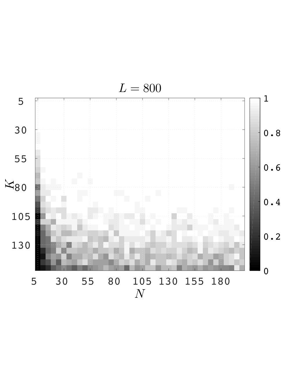
We present phase transitions that validate the sample complexity results in Theorem 1. The shade in the phase transitions represents the probability of failure determined by counting the frequency of failures in twenty five experiments for each pixel in the phase transitions. We classify the recovered solution 𝑿^\hat{\bm{X}} as a failure if ‖𝑿^−𝒉​𝒎∗‖F>10−1\|\hat{\bm{X}}-\bm{h}\bm{m}^{*}\|_{{\operatorname{F}}}>10^{-1}.

In all of the phase transitions, we take 𝒘\bm{w}, and 𝒎\bm{m} to be Gaussian vectors. Observe that 𝒘\bm{w} is constructed to be a dense vector with no sparse model. Recall that Theorem 1 restricts 𝒘\bm{w} to be a sparse vector, however, our simulation results show successful recovery in a more general case of dense 𝒘\bm{w}. This observation is in conformation with our belief that the sparsity assumption on 𝒘\bm{w} is a result of merely a technical requirement due to the proof method. Very similar phase transitions can be obtained under restrictive sparse model on 𝒘\bm{w}.

We will present two sets of phase transitions. Each set contains three phase transition diagrams; in each diagram, we fix one of the variables LL, KK, and NN, and vary the other two in small increments and compute the probability of failure every time as outlined earlier in this section.

In the first set, we mimic the channel estimation problem discussed in Section 1.4, and shown in Figure 1. We take 𝑪n\bm{C}_{n}’s to be Gaussian matrices as in (11). Figure 3 shows that for a fixed N=40N=40, we are able to recover all of the inputs 𝒙n\bm{x}_{n}’s, and 𝒘\bm{w} as soon as L≥10​KL\geq 10K. The phase diagrams in Figure 3 and 3 mainly show that the performance of the algorithm become roughly oblivious to the number NN of inputs as soon as N≥10N\geq 10 for the particular range of KK, and LL considered in the phase transition diagrams.

In the second set shown in Figure 4, we simulate the blind channel estimation problem discussed in Section 1.5, and shown in Figure 2. This set contains similar phase diagrams as in first set under the same assumptions, the only difference is that the matrices 𝑪n\bm{C}_{n}’s are now the random subsets of the columns of identity. In other words, we take the support of 𝒙n\bm{x}_{n}’s to be random and known. The results are almost exactly the same as in the first set.

Refer to caption
Refer to caption
Refer to caption
Figure 3: Empirical success rate for the deconvolution of 𝒘\bm{w} and 𝒙1,𝒙2,…,𝒙N\bm{x}_{1},\bm{x}_{2},\ldots,\bm{x}_{N}. Recall that 𝒙n=𝑪n​𝒎n\bm{x}_{n}=\bm{C}_{n}\bm{m}_{n} for every n=1,2,3,…,Nn=1,2,3,\ldots,N. In these experiments, the vectors 𝒘\bm{w}, 𝒎n\bm{m}_{n} are Gaussian, and L×KL\times K matrices 𝑪n,n=1,2,3,…,N\bm{C}_{n},n=1,2,3,\ldots,N are also independent, and Gaussian. (a) Fix N=40N=40, and vary L∼200→2000L\sim 200\rightarrow 2000, K∼10→190K\sim 10\rightarrow 190. Successful reconstruction is obtained with probability one when L≥10​KL\geq 10K. (b) Fix L=800L=800, and vary K∼5→150K\sim 5\rightarrow 150, N∼5→200N\sim 5\rightarrow 200. Successful reconstruction is obtained with probability one when K≤L/10K\leq L/10, and N≥10N\geq 10. (c) Fix K=40K=40, and vary L∼50→800L\sim 50\rightarrow 800, N∼10→200N\sim 10\rightarrow 200. Successful reconstruction occurs with probability one when L≥10​KL\geq 10K, and N≥10N\geq 10.
Refer to caption
Refer to caption
Refer to caption
Figure 4: Empirical success rate for the deconvolution of 𝒘\bm{w} and 𝒙1,𝒙2,…,𝒙N\bm{x}_{1},\bm{x}_{2},\ldots,\bm{x}_{N}. In these experiments, the vector 𝒘\bm{w} is Gaussian, and every 𝒙n\bm{x}_{n} is a sparse vector with random support and its KK non-zero entries are Gaussian. (a) Fix N=40N=40, and vary L∼200→2000L\sim 200\rightarrow 2000, K∼10→190K\sim 10\rightarrow 190. Successful reconstruction is obtained with probability one when L≥10​KL\geq 10K. (b) Fix L=800L=800, and vary K∼5→150K\sim 5\rightarrow 150, N∼5→200N\sim 5\rightarrow 200. Successful reconstruction is obtained with probability one when K≤L/10K\leq L/10, and N≥10N\geq 10. (c) Fix K=40K=40, and vary L∼50→800L\sim 50\rightarrow 800, N∼10→200N\sim 10\rightarrow 200. Successful reconstruction occurs with probability one when L≥10​KL\geq 10K, and N≥10N\geq 10.

3 Proof of Theorem 1

We are observing the linear measurements as in (5) of an unknown 𝑿0=𝒉​𝒎∗\bm{X}_{0}=\bm{h}\bm{m}^{*} such that 𝒉\bm{h} is an SS-sparse vector. Define Ω:=supp​(𝒉)\Omega:=\mbox{supp}(\bm{h}), where |Ω|=S|\Omega|=S. To show that the solution to the SDP in (8) equals 𝑿0\bm{X}_{0} with high probability, we establish the existence of a valid dual certificate [7, 15]. The proof of low-rank recovery using dual certificate method is a standard approach now and has been employed in the literature [2, 23, 15] many times before. Our construction of the dual certificate uses the golfing scheme [15], but is unusually technical in that there is a probabilistic dependence between the iterates, which in turn precludes the use of matrix concentration inequalities.

Let 𝒖∈ℝL\bm{u}\in\mathbb{R}^{L}, and 𝒗∈ℝK​N\bm{v}\in\mathbb{R}^{KN} be arbitrary vectors, and 𝒉\bm{h}, and 𝒎\bm{m} be as defined earlier. Let T1T_{1} be the linear space of matrices with rank at most two defined as

T1:={𝑿|𝑿=α𝒉𝒗∗+β𝒖𝒎∗,andα,β∈ℝ},T_{1}:=\{\bm{X}|\bm{X}=\alpha\bm{h}\bm{v}^{*}+\beta\bm{u}\bm{m}^{*},~\mbox{and}~\alpha,\beta\in\mathbb{R}\},

and T2T_{2} be the space of matrices with rows supported on index set Ω\Omega, and is defined as

T2:={𝑿|𝑿∈ℝL×K​N,X[ℓ,j]=0forℓ∈Ω⟂},T_{2}:=\{\bm{X}~|~\bm{X}\in\mathbb{R}^{L\times KN},X[\ell,j]=0~\mbox{for}~\ell\in\Omega^{\perp}\},

where Ω⟂=[L]\Ω\Omega^{\perp}=[L]\backslash\Omega. Then we have

T1∩T2:={𝑿|𝑿=α𝒉𝒗∗+β𝒖𝒎∗,𝒖Ω⟂=𝟎,andα,β∈ℝ}.T_{1}\cap T_{2}:=\{\bm{X}|\bm{X}=\alpha\bm{h}\bm{v}^{*}+\beta\bm{u}\bm{m}^{*},\bm{u}_{\Omega^{\perp}}=\bm{0},~\mbox{and}~\alpha,\beta\in\mathbb{R}\}.

Note that the matrix of interest 𝑿0\bm{X}_{0} is a member of the space T1∩T2T_{1}\cap T_{2}. Let us now define the related projection operators. We start by defining 𝒫\mathcal{P} that takes a matrix or a vector with LL rows and sets all the rows that are not indexed by the index set Ω⊂[L]\Omega\subset[L] to zero. Mathematically, we can define the projection on the index set Ω\Omega as

𝒫⁡(𝑿):=𝑰L×Ω​𝑰L×Ω∗​𝑿\mathcal{P}(\bm{X}):=\bm{I}_{L\times\Omega}\bm{I}_{L\times\Omega}^{*}\bm{X} (14)

where 𝑰L×Ω\bm{I}_{L\times\Omega} denotes the submatrix of the L×LL\times L identity matrix with columns indexed by set Ω\Omega. The orthogonal projector ℛ\mathcal{R} onto T1∩T2T_{1}\cap T_{2} is then defined as

ℛ⁡(𝒁):=𝒉​𝒉∗​𝒁+𝒫⁡(𝒁​𝒎​𝒎∗)−𝒉​𝒉∗​𝒁​𝒎​𝒎∗,\mathcal{R}(\bm{Z}):=\bm{h}\bm{h}^{*}\bm{Z}+\mathcal{P}(\bm{Z}\bm{m}\bm{m}^{*})-\bm{h}\bm{h}^{*}\bm{Z}\bm{m}\bm{m}^{*}, (15)

and the projector ℛ⟂\mathcal{R}_{\scalebox{0.6}{$\perp$}} onto the orthogonal complement T1⟂∪T2⟂T_{1}^{\perp}\cup T_{2}^{\perp} of T1∩T2T_{1}\cap T_{2} is then simply ℛ⟂​(𝒁)=𝒁−ℛ⁡(𝒁)\mathcal{R}_{\scalebox{0.6}{$\perp$}}(\bm{Z})=\bm{Z}-\mathcal{R}(\bm{Z}). Note that in the definition of the projection above, we assume without loss of generality that ‖𝒎‖2=‖𝒉‖2=1\|\bm{m}\|_{2}=\|\bm{h}\|_{2}=1 as the optimality conditions, presented in Lemma 1 below, for the success of nuclear norm minimization 8 only involve normalized 𝒉\bm{h}, and 𝒎\bm{m}.

The following lemma gives sufficient conditions on a dual certificate 𝒀∈Range​(𝒜∗)\bm{Y}\in\text{Range}(\mathcal{A}^{*}) to guarantee that nuclear-norm minimization program in (8) produces 𝑿0=𝒉​𝒎∗\bm{X}_{0}=\bm{h}\bm{m}^{*} as the solution. The proof of the lemma is almost exactly the same as in [7], the only difference is that now instead of just working with a space of rank-2 matrices T1T_{1}, we are dealing with the space T1∩T2T_{1}\cap T_{2} of rank-2 and row-sparse matrices. We repeat the proof here to show that all the details in [7] also work out for the space T1∩T2T_{1}\cap T_{2}.

Lemma 1 (Optimality Conditions).

Let 𝒜\mathcal{A} be as defined in (7), and γ>0\gamma>0 be a positive number such that ‖𝒜‖≤γ\|\mathcal{A}\|\leq\gamma, and

2​‖𝒜​ℛ​(𝒁)‖F≥‖ℛ⁡(𝒁)‖F\sqrt{2}\|\mathcal{A}\mathcal{R}(\bm{Z})\|_{\operatorname{F}}\geq\|\mathcal{R}(\bm{Z})\|_{\operatorname{F}} (16)

for all 𝐙∈Null​(𝒜)\bm{Z}\in\mbox{Null}(\mathcal{A}). Then the matrix 𝐗0=𝐡​𝐦∗\bm{X}_{0}=\bm{h}\bm{m}^{*} is the unique minimizer of (8) if there exists a 𝐘∈Range​(𝒜∗)\bm{Y}\in\mbox{Range}(\mathcal{A}^{*}) such that

‖𝒉​𝒎∗−ℛ⁡(𝒀)‖F≤14​γ,‖ℛ⟂​(𝒀)‖≤12.\|\bm{h}\bm{m}^{*}-\mathcal{R}(\bm{Y})\|_{\operatorname{F}}\leq\frac{1}{4\gamma},\qquad\|\mathcal{R}_{\scalebox{0.6}{$\perp$}}(\bm{Y})\|\leq\frac{1}{2}. (17)
Proof.

Let 𝑿^\hat{\bm{X}} denote the solution to the optimization program in (8). This implies that ‖𝑿^‖∗≤‖𝑿0‖∗\|\hat{\bm{X}}\|_{*}\leq\|\bm{X}_{0}\|_{*}. Given this, it is enough to show

‖𝑿0+𝒁‖∗>‖𝑿0‖∗,∀𝒁∈Null​(𝒜),𝒁≠𝟎,\|\bm{X}_{0}+\bm{Z}\|_{*}>\|\bm{X}_{0}\|_{*},~\forall\bm{Z}\in\mbox{Null}(\mathcal{A}),~\bm{Z}\neq\bm{0},

where 𝒁=𝑿^−𝑿0\bm{Z}=\hat{\bm{X}}-\bm{X}_{0}, to establish exact recovery, since the two conflicting requirements on 𝑿^\hat{\bm{X}} above would directly mean that 𝑿^=𝑿0\hat{\bm{X}}=\bm{X}_{0}, or 𝒁=𝟎\bm{Z}=\bm{0}.

The sub-differential of nuclear norm at point 𝑿0\bm{X}_{0} is (see [32] for details)

∂∥𝑿0∥∗:={𝒉𝒎∗+𝑾:ℛ⟂(𝑾)=𝑾,and∥𝑾∥≤1}.\partial\|\bm{X}_{0}\|_{*}:=\{\bm{h}\bm{m}^{*}+\bm{W}:\mathcal{R}_{\scalebox{0.6}{$\perp$}}(\bm{W})=\bm{W},~\mbox{and}~\|\bm{W}\|\leq 1\}.

Since by the definition of sub-differentials

‖𝑿0+𝒁‖∗−‖𝑿0‖∗≥⟨𝚫,𝒁⟩, for every ​𝚫∈∂‖𝑿0‖∗,\|\bm{X}_{0}+\bm{Z}\|_{*}-\|\bm{X}_{0}\|_{*}\geq\langle\bm{\Delta},\bm{Z}\rangle,~\mbox{ for every }\bm{\Delta}\in\partial\|\bm{X}_{0}\|_{*},

we obtain

‖𝑿0+𝒁‖∗−‖𝑿0‖∗\displaystyle\|\bm{X}_{0}+\bm{Z}\|_{*}-\|\bm{X}_{0}\|_{*} ≥⟨𝒉​𝒎∗,𝒁⟩+⟨ℛ⟂​(𝑾),𝒁⟩\displaystyle\geq\langle\bm{h}\bm{m}^{*},\bm{Z}\rangle+\langle\mathcal{R}_{\scalebox{0.6}{$\perp$}}(\bm{W}),\bm{Z}\rangle
=⟨𝒉​𝒎∗−𝒀,𝒁⟩+⟨𝑾,ℛ⟂​(𝒁)⟩, for every ​𝒀∈Range​(𝒜∗).\displaystyle=\langle\bm{h}\bm{m}^{*}-\bm{Y},\bm{Z}\rangle+\langle\bm{W},\mathcal{R}_{\scalebox{0.6}{$\perp$}}(\bm{Z})\rangle,~\mbox{ for every }\bm{Y}\in\mbox{Range}(\mathcal{A}^{*}).

Using the fact that 𝒉​𝒎∗∈T1∩T2\bm{h}\bm{m}^{*}\in T_{1}\cap T_{2}, and also maximizing the inner product ⟨𝑾,ℛ⟂​(𝒁)⟩\langle\bm{W},\mathcal{R}_{\scalebox{0.6}{$\perp$}}(\bm{Z})\rangle with respect to ‖𝑾‖≤1\|\bm{W}\|\leq 1 gives us

‖𝑿0+𝒁‖∗−‖𝑿0‖∗\displaystyle\|\bm{X}_{0}+\bm{Z}\|_{*}-\|\bm{X}_{0}\|_{*} ≥⟨𝒉​𝒎∗−ℛ⁡(𝒀),ℛ⁡(𝒁)⟩−⟨ℛ⟂​(𝒀),ℛ⟂​(𝒁)⟩+‖ℛ⟂​(𝒁)‖∗\displaystyle\geq\langle\bm{h}\bm{m}^{*}-\mathcal{R}(\bm{Y}),\mathcal{R}(\bm{Z})\rangle-\langle\mathcal{R}_{\scalebox{0.6}{$\perp$}}(\bm{Y}),\mathcal{R}_{\scalebox{0.6}{$\perp$}}(\bm{Z})\rangle+\|\mathcal{R}_{\scalebox{0.6}{$\perp$}}(\bm{Z})\|_{*}
≥−‖𝒉​𝒎∗−ℛ⁡(𝒀)‖F​‖ℛ⁡(𝒁)‖F−‖ℛ⟂​(𝒀)‖​‖ℛ⟂​(𝒁)‖∗+‖ℛ⟂​(𝒁)‖∗.\displaystyle\geq-\|\bm{h}\bm{m}^{*}-\mathcal{R}(\bm{Y})\|_{\operatorname{F}}\|\mathcal{R}(\bm{Z})\|_{\operatorname{F}}-\|\mathcal{R}_{\scalebox{0.6}{$\perp$}}(\bm{Y})\|\|\mathcal{R}_{\scalebox{0.6}{$\perp$}}(\bm{Z})\|_{*}+\|\mathcal{R}_{\scalebox{0.6}{$\perp$}}(\bm{Z})\|_{*}.

Now the inequality ∥𝒜ℛ(𝒁)∥F≥2−1/2∥ℛ(𝒁)∥F\|\mathcal{A}\mathcal{R}(\bm{Z})\|_{\operatorname{F}}\geq 2^{-1/2}\|\mathcal{R}(\bm{Z})\|_{\operatorname{F}} for any 𝒁∈Null​(𝒜)\bm{Z}\in\mbox{Null}(\mathcal{A}) implies that

0=‖𝒜⁡(𝒁)‖F\displaystyle 0=\|\mathcal{A}(\bm{Z})\|_{\operatorname{F}} ≥‖𝒜​ℛ​(𝒁)‖F−‖𝒜​ℛ⟂​(𝒁)‖F\displaystyle\geq\|\mathcal{A}\mathcal{R}(\bm{Z})\|_{\operatorname{F}}-\|\mathcal{A}\mathcal{R}_{\scalebox{0.6}{$\perp$}}(\bm{Z})\|_{\operatorname{F}}
≥2−1/2∥ℛ(𝒁)∥F−γ∥ℛ⟂(𝒁)∥F.\displaystyle\geq 2^{-1/2}\|\mathcal{R}(\bm{Z})\|_{\operatorname{F}}-\gamma\|\mathcal{R}_{\scalebox{0.6}{$\perp$}}(\bm{Z})\|_{\operatorname{F}}.

The above inequality implies firstly that ‖𝒁‖F2≤(2​γ2+1)​‖ℛ⟂​(𝒁)‖F2\|\bm{Z}\|_{\operatorname{F}}^{2}\leq(2\gamma^{2}+1)\|\mathcal{R}_{\scalebox{0.6}{$\perp$}}(\bm{Z})\|_{\operatorname{F}}^{2}, which in turn means ℛ⟂​(𝒁)≠𝟎\mathcal{R}_{\scalebox{0.6}{$\perp$}}(\bm{Z})\neq\bm{0} whenever 𝒁≠𝟎\bm{Z}\neq\bm{0}; secondly, ‖ℛ⁡(𝒁)‖F≤2​γ​‖ℛ⟂​(𝒁)‖∗\|\mathcal{R}(\bm{Z})\|_{\operatorname{F}}\leq\sqrt{2}\gamma\|\mathcal{R}_{\scalebox{0.6}{$\perp$}}(\bm{Z})\|_{*}. Using these results, the bound in the earlier inequality gives

‖𝑿0+𝒁‖∗−‖𝑿0‖∗≥(−‖𝒉​𝒎∗−ℛ⁡(𝒀)‖F​2​γ−‖ℛ⟂​(𝒀)‖+1)​‖ℛ⟂​(𝒁)‖∗.\|\bm{X}_{0}+\bm{Z}\|_{*}-\|\bm{X}_{0}\|_{*}\geq\left(-\|\bm{h}\bm{m}^{*}-\mathcal{R}(\bm{Y})\|_{\operatorname{F}}\sqrt{2}\gamma-\|\mathcal{R}_{\scalebox{0.6}{$\perp$}}(\bm{Y})\|+1\right)\|\mathcal{R}_{\scalebox{0.6}{$\perp$}}(\bm{Z})\|_{*}.

Now under the conditions in (17), the right hand side above is strictly positive, which means ‖𝑿0+𝒁‖∗>‖𝑿0‖∗\|\bm{X}_{0}+\bm{Z}\|_{*}>\|\bm{X}_{0}\|_{*}; enough to exhibit the uniqueness. ∎

The next lemma provides an upper bound γ\gamma on the operator norm of the linear map 𝒜\mathcal{A}.

Lemma 2 (Operator norm of 𝒜\mathcal{A}).

Let 𝒜\mathcal{A} be as defined in (7). For any β≥1\beta\geq 1,

‖𝒜‖≤β​K​log⁡(L​N)\|\mathcal{A}\|\leq\sqrt{\beta K\log(LN)}

with probability at least 1−(L​N)−β+21-(LN)^{-\beta+2}.

Proof.

The operator norm can be calculated by using the fact that ⟨𝑨ℓ1,n1,𝑨ℓ2,n2⟩=0\langle\bm{A}_{\ell_{1},n_{1}},\bm{A}_{\ell_{2},n_{2}}\rangle=0,  ∀ℓ1≠ℓ2∈[L]\forall\ell_{1}\neq\ell_{2}\in[L], or ∀n1≠n2∈[N]\forall n_{1}\neq n_{2}\in[N]. This implies that ‖𝒜‖=maxℓ,n⁡‖𝑨ℓ,n‖F\|\mathcal{A}\|=\max_{\ell,n}\|\bm{A}_{\ell,n}\|_{\operatorname{F}}. We can write ∥𝑨ℓ,n∥F2=∥𝒃ℓ∥22∥ϕℓ,n∥22=∑k∼Kn|cℓ,n[k]|2\|\bm{A}_{\ell,n}\|^{2}_{\operatorname{F}}=\|{\bm{b}}_{\ell}\|^{2}_{2}\|\bm{\phi}_{\ell,n}\|^{2}_{2}=\sum_{k\sim_{K}n}|c_{\ell,n}[k]|^{2}, where |cℓ,n​[k]|2|c_{\ell,n}[k]|^{2} are chi-squared random variables with degree 2 when 2≤ℓ≤L/22\leq\ell\leq L/2, and degree 1 when ℓ=1\ell=1, or ℓ=L/2+1\ell=L/2+1. In both cases E⁡|cℓ,n​[k]|2=1\operatorname{{E}}|c_{\ell,n}[k]|^{2}=1, and

ℙ{|cℓ,n[k]|2>u}≤e−u.\displaystyle\operatorname{\mathbb{P}}\{|c_{\ell,n}[k]|^{2}>u\}\leq\mathrm{e}^{-u}.

The maximum is taken over (L/2+1)⋅2⋅K​N(L/2+1)\cdot 2\cdot KN unique cℓ,n​[k]c_{\ell,n}[k] and

ℙ{maxℓ,n,k|cℓ,n[k]|2≥u}≤(L+2)KN⋅e−u⇒ℙ{maxℓ,n∥𝑨ℓ,n∥F2≥Ku}≤(LN)2e−u,\displaystyle\operatorname{\mathbb{P}}\{\max_{\ell,n,k}|c_{\ell,n}[k]|^{2}\geq u\}\leq(L+2)KN\cdot\mathrm{e}^{-u}\Rightarrow\operatorname{\mathbb{P}}\{\max_{\ell,n}\|\bm{A}_{\ell,n}\|_{\operatorname{F}}^{2}\geq Ku\}\leq(LN)^{2}e^{-u},

where the last inequality follows from the fact that K≤LK\leq L. Choose u=β​log⁡(L​N)u=\beta\log(LN), which gives ‖𝒜‖≤γ:=β​K​log⁡(L​N)\|\mathcal{A}\|\leq\gamma:=\sqrt{\beta K\log(LN)} with probability at least 1−(L​N)−β+21-(LN)^{-\beta+2}. ∎

In the following section, we focus on constructing a dual certificating using golfing scheme, which is then shown to satisfy the uniqueness conditions in the lemma above.

3.1 Linear operators on golfing partition

To prove the uniqueness conditions in (17), we use a dual certificate 𝒀\bm{Y} constructed using a variation of the golfing scheme [15]. To this end, we partition the index set [L]×[N][L]\times[N] into PP disjoint sets Γ1,Γ2,…,ΓP\Gamma_{1},\Gamma_{2},\ldots,\Gamma_{P} defined as

Γp:={(ℓ,n)|(ℓ,n)∈{(Δn,p,n)}n=1N},\displaystyle\Gamma_{p}:=\left\{(\ell,n)~|~(\ell,n)\in\{(\Delta_{n,p},n)\}_{n=1}^{N}\right\}, (18)

where Δn,p\Delta_{n,p} is a subset of [L][L], chosen uniformly at random for every nn and pp, such that |Δn,p|=Q=L/P|\Delta_{n,p}|=Q=L/P, and for every nn, Δn,p∩Δn,p′=∅\Delta_{n,p}\cap\Delta_{n,p^{\prime}}=\emptyset for p≠p′p\neq p^{\prime}, and ⋃pΔn,p=[L]\bigcup_{p}\Delta_{n,p}=[L]. The parameter QQ is adjusted through the proof, and we assume here without loss of generality that it is an integer33 3 We are assuming here that PP is a factor of LL; this can be achieved in the worst case by increasing the number LL of measurements in each convolution by no more than a factor 2, which only affects the measurements bounds in Theorem 1 by a multiplicative constant.. In words, the partition of the set {1,2,3,…,L}×{1,2,3,…,N}\{1,2,3,\ldots,L\}\times\{1,2,3,\ldots,N\} is obtained by dividing {1,2,3,…,L}\{1,2,3,\ldots,L\} into PP randomly chosen disjoint sets for a given nn, and then we repeat this process independently for every nn to obtain a total of P​NPN sets Δ1,1,…,ΔN,1,Δ1,2,…,ΔN,P\Delta_{1,1},\ldots,\Delta_{N,1},\Delta_{1,2},\ldots,\Delta_{N,P}. We then define Γp\Gamma_{p} as in (18). For every nn, the disjointness among the sets Δn,1,Δn,2,…,Δn,P\Delta_{n,1},\Delta_{n,2},\ldots,\Delta_{n,P} is of critical importance as it ensures that no dependence arises due to reuse of the same ϕℓ,n\bm{\phi}_{\ell,n} in different partitioned sets. We define a linear map 𝒜p:ℝL×K​N→ℂQ​N\mathcal{A}_{p}:\mathbb{R}^{L\times KN}\rightarrow\mathbb{C}^{QN} that returns the measurements indexed by (ℓ,n)∈Γp(\ell,n)\in\Gamma_{p}:

𝒜p​(𝒁):={⟨𝒃ℓ​ϕℓ,n∗,𝒁⟩:(ℓ,n)∈Γp},𝒜p∗​𝒜p​(𝒁):=∑(ℓ,n)∈Γp⟨𝒃ℓ​ϕℓ,n∗,𝒁⟩​𝒃ℓ​ϕℓ,n∗.\displaystyle\mathcal{A}_{p}(\bm{Z}):=\{\langle{\bm{b}}_{\ell}\bm{\phi}_{\ell,n}^{*},\bm{Z}\rangle:(\ell,n)\in\Gamma_{p}\},~~~~~~\mathcal{A}_{p}^{*}\mathcal{A}_{p}(\bm{Z}):=\sum_{(\ell,n)\in\Gamma_{p}}\langle{\bm{b}}_{\ell}\bm{\phi}_{\ell,n}^{*},\bm{Z}\rangle{\bm{b}}_{\ell}\bm{\phi}_{\ell,n}^{*}. (19)

In tandem with this partitioning of the measurements, we also require to partition the LL rows of 𝑩^\hat{\bm{B}} into PP sets of Q×LQ\times L submatrices that behave roughly as an isometry on the sparse vectors. Quantitatively, we want the rows 𝒃ℓ∗{\bm{b}}_{\ell}^{*} of matrix 𝑩^\hat{\bm{B}} in each of the sets Δn,p\Delta_{n,p} to obey

(1−δ)​‖𝒛‖22≤LQ​∑ℓ∈Δn,p|𝒃ℓ∗​𝒛|2≤(1+δ)​‖𝒛‖22\displaystyle(1-\delta)\|\bm{z}\|_{2}^{2}\leq\frac{L}{Q}\sum_{\ell\in\Delta_{n,p}}|{\bm{b}}_{\ell}^{*}\bm{z}|^{2}\leq(1+\delta)\|\bm{z}\|_{2}^{2} (20)

for all vectors 𝒛\bm{z} supported on the set Ω\Omega such that |Ω|≤S|\Omega|\leq S. A reader familiar with compressive sensing will readily recognize this as the restricted isometry property (RIP) [5] on the submatrices of 𝑩^\hat{\bm{B}}. A result [26] from compressive sensing says that for each submatrix of rows 𝒃ℓ{\bm{b}}_{\ell} with coherence μmax2\mu^{2}_{\max}, defined in (9) if the index set Δn,p\Delta_{n,p} is chosen uniformly at random, then there exists a constant CC such that for any 0<δ<10<\delta<1, and 0<ϵ<10<\epsilon<1,

Q≥C​δ−1​μmax2​(S​log⁡Lϵ2)​log⁡(S​log⁡Lϵ2)​log2​S\displaystyle Q\geq C\delta^{-1}\mu_{\max}^{2}\left(\frac{S\log L}{\epsilon^{2}}\right)\log\left(\frac{S\log L}{\epsilon^{2}}\right)\log^{2}S

implies that the RIP in (20) holds with probability exceeding 1−e−c​(δ/ϵ)21-e^{-c(\delta/\epsilon)^{2}}. Given the partition {Δn,p}n,p\{\Delta_{n,p}\}_{n,p} is chosen uniformly at random, the above result with δ=1/4\delta=1/4, and ϵ−2=β​log⁡(L​N)\epsilon^{-2}=\beta\log(LN) means that if

Q≥C​β​μmax2​S​log2⁡(L​N)​log⁡(β​S​log⁡(L​N))​log2​S,\displaystyle Q\geq C\beta\mu_{\max}^{2}S\log^{2}(LN)\log(\beta S\log(LN))\log^{2}S, (21)

then

sup|Ω|≤S∑ℓ∈Δn,p|𝒃ℓ∗​𝒛|2≤5​Q4​L​‖𝒛‖22,\displaystyle\sup_{|\Omega|\leq S}\sum_{\ell\in\Delta_{n,p}}|{\bm{b}}_{\ell}^{*}\bm{z}|^{2}\leq\frac{5Q}{4L}\|\bm{z}\|_{2}^{2},

with probability at least 1−𝒪⁡((L​N)−β)1-\mathcal{O}((LN)^{-\beta}), for all 𝒛\bm{z} supported on Ω\Omega for a given Δn,p\Delta_{n,p}. A simple union bound over all P​NPN number of sets {Δn,p}n,p\{\Delta_{n,p}\}_{n,p} shows that

maxn,p⁡[sup|Ω|≤S∑ℓ∈Δn,p|𝒃ℓ∗​𝒛|2]≤5​Q4​L​‖𝒛‖22⟹maxn,p⁡‖∑ℓ∈Δn,p𝒫​𝒃ℓ​𝒃ℓ∗​𝒫−QL​𝒫‖≤Q4​L\displaystyle\max_{n,p}\left[\sup_{|\Omega|\leq S}\sum_{\ell\in\Delta_{n,p}}|{\bm{b}}_{\ell}^{*}\bm{z}|^{2}\right]\leq\frac{5Q}{4L}\|\bm{z}\|_{2}^{2}\implies\max_{n,p}\left\|\sum_{\ell\in\Delta_{n,p}}\mathcal{P}{\bm{b}}_{\ell}{\bm{b}}_{\ell}^{*}\mathcal{P}-\frac{Q}{L}\mathcal{P}\right\|\leq\frac{Q}{4L} (22)

holds with probability at least 1−(P​N)​𝒪​((L​N)−β)≥1−𝒪⁡((L​N)1−β)1-(PN)\mathcal{O}((LN)^{-\beta})\geq 1-\mathcal{O}((LN)^{1-\beta}). In the rest of the article, we take the results in (22) as given.

Before constructing a dual certificate, we define some nomenclature. Let

𝑺n,p:=∑ℓ∈Δn,p(𝒫​𝒃ℓ)​(𝒫​𝒃ℓ)∗,and​𝑺n,p‡:=𝑰L×Ω​(𝑰L×Ω∗​𝑺n,p​𝑰L×Ω)−1​𝑰L×Ω∗,\displaystyle\bm{S}_{n,p}:=\sum_{\ell\in\Delta_{n,p}}(\mathcal{P}{\bm{b}}_{\ell})(\mathcal{P}{\bm{b}}_{\ell})^{*},~\mbox{and}~\bm{S}_{n,p}^{\ddagger}:=\bm{I}_{L\times\Omega}\left(\bm{I}_{L\times\Omega}^{*}\bm{S}_{n,p}\bm{I}_{L\times\Omega}\right)^{-1}\bm{I}_{L\times\Omega}^{*}, (23)

where 𝑰L×Ω\bm{I}_{L\times\Omega} is an L×|Ω|L\times|\Omega| matrix containing the columns of an L×LL\times L identity matrix indexed by set Ω\Omega. A direct conclusion of (22) gives

maxn,p⁡‖𝑺n,p‖≤5​Q4​L,maxn,p⁡‖𝑺n,p‡‖≤4​L3​Q.\displaystyle\max_{n,p}\|\bm{S}_{n,p}\|\leq\frac{5Q}{4L},~~\max_{n,p}\|\bm{S}_{n,p}^{\ddagger}\|\leq\frac{4L}{3Q}. (24)

In addition, set 𝑫n=𝑰K⊗𝒆n​𝒆n∗.\bm{D}_{n}=\bm{I}_{K}\otimes\bm{e}_{n}\bm{e}_{n}^{*}. A linear operator 𝒮p‡\mathcal{S}_{p}^{\ddagger} is then defined by its action on an L×K​NL\times KN matrix 𝑿\bm{X} as follows

𝒮p‡​(𝑿)=∑n𝑺n,p‡​𝑿​𝑫n.\mathcal{S}_{p}^{\ddagger}(\bm{X})=\sum_{n}\bm{S}_{n,p}^{\ddagger}\bm{X}\bm{D}_{n}. (25)

3.2 Coherence

With all the development above, we are now in position to precisely define the coherence parameter μ02\mu_{0}^{2} that was first introduced in Section 1.3. The diffusion of the impulse response 𝒘\bm{w} is quantified using the following definition

μ02:=L⋅max⁡{‖𝑩^​𝒉‖∞2‖𝒉‖22,Q2L2⋅maxn,p⁡‖𝑩^​𝑺n,p‡​𝒉‖∞2‖𝒉‖22,maxn,n′⁡‖𝑩^​𝑺n,2‡​𝑺n′,1​𝒉‖∞2‖𝒉‖22}.\displaystyle\mu_{0}^{2}:=L\cdot\max\left\{\frac{\|\hat{\bm{B}}\bm{h}\|_{\infty}^{2}}{\|\bm{h}\|_{2}^{2}},\frac{Q^{2}}{L^{2}}\cdot\max_{n,p}\frac{\|\hat{\bm{B}}\bm{S}_{n,p}^{\ddagger}\bm{h}\|_{\infty}^{2}}{\|\bm{h}\|_{2}^{2}},\max_{n,n^{\prime}}\frac{\|\hat{\bm{B}}\bm{S}^{\ddagger}_{n,2}\bm{S}_{n^{\prime},1}\bm{h}\|_{\infty}^{2}}{\|\bm{h}\|_{2}^{2}}\right\}. (26)

The quantities 𝒉n,n′′′\bm{h}^{\prime\prime}_{n,n^{\prime}} and 𝒉n,n′′′\bm{h}^{\prime\prime}_{n,n^{\prime}} from Section 1.3 can be easily read off from this expression, and from ℓ2\ell_{2} norm equivalences resulting from (24)44 4 So that μ02\mu_{0}^{2} as defined here, and its illustration listed in the introduction, are equivalent to within an inconsequential multiplicative factor.. The following lemma presents upper and lower bounds on μ02\mu_{0}^{2}.

Lemma 3 (Range of μ02\mu_{0}^{2}).

Let μ02\mu_{0}^{2}, and μmax2\mu_{\max}^{2} be as defined in (26), and (9), respectively. Assume that (24) holds. Then

53≤μ02≤209​μmax2​S.\frac{5}{3}\leq\mu_{0}^{2}\leq\frac{20}{9}\mu_{\max}^{2}S.
Proof.

We assume without loss of generality that ‖𝒉‖22=1\|\bm{h}\|_{2}^{2}=1. Since 𝑩^\hat{\bm{B}} is an orthonormal matrix, it is easy to see that 1/L≤‖𝑩^​𝒉‖∞2≤11/L\leq\|\hat{\bm{B}}\bm{h}\|_{\infty}^{2}\leq 1. As far as ‖𝑩^​𝑺n,p‡​𝒉‖∞2\|\hat{\bm{B}}\bm{S}_{n,p}^{\ddagger}\bm{h}\|_{\infty}^{2} is concerned, an upper bound on it is

maxn,p⁡‖𝑩^​𝑺n,p‡​𝒉‖∞2\displaystyle\max_{n,p}\|\hat{\bm{B}}\bm{S}_{n,p}^{\ddagger}\bm{h}\|_{\infty}^{2} =maxℓ⁡maxn,p​|𝒃ℓ∗​𝑺n,p‡​𝒉|2≤maxℓ⁡‖𝒃ℓ‖∞2​maxn,p​‖𝑺n,p‡​𝒉‖12\displaystyle=\max_{\ell}\max_{n,p}|{\bm{b}}_{\ell}^{*}\bm{S}_{n,p}^{\ddagger}\bm{h}|^{2}\leq\max_{\ell}\|{\bm{b}}_{\ell}\|_{\infty}^{2}\max_{n,p}\|\bm{S}_{n,p}^{\ddagger}\bm{h}\|_{1}^{2}
≤μmax2​1L​S​‖𝑺n,p‡​𝒉‖22≤169​μmax2​S​LQ2,\displaystyle\leq\mu_{\max}^{2}\frac{1}{L}S\|\bm{S}_{n,p}^{\ddagger}\bm{h}\|_{2}^{2}\leq\frac{16}{9}\mu_{\max}^{2}S\frac{L}{Q^{2}},

where the first inequality is Hölder’s result; the second one follows from the definition of coherence μmax2\mu_{\max}^{2} in (9), the equivalence of ℓ1\ell_{1}, and ℓ2\ell_{2}-norms, and the fact that the vector 𝑺n,p‡​𝒉\bm{S}_{n,p}^{\ddagger}\bm{h} is SS-sparse; and the last one is the result of (24). A lower bound can be obtained by summing over ℓ∈[L]\ell\in[L] as follows:

L⋅maxℓ⁡maxn,p​|𝒃ℓ∗​𝑺n,p‡​𝒉|2≥max⁡∑ℓn,p⁡|𝒃ℓ∗​𝑺n,p‡​𝒉|2=maxn,p⁡‖𝑺n,p‡​𝒉‖22≥1625​L2Q2,L\cdot\max_{\ell}\max_{n,p}|{\bm{b}}_{\ell}^{*}\bm{S}_{n,p}^{\ddagger}\bm{h}|^{2}\geq\max_{n,p}\sum_{\ell}|{\bm{b}}_{\ell}^{*}\bm{S}_{n,p}^{\ddagger}\bm{h}|^{2}=\max_{n,p}\|\bm{S}_{n,p}^{\ddagger}\bm{h}\|_{2}^{2}\geq\frac{16}{25}\frac{L^{2}}{Q^{2}},

where the equality is due to the fact that 𝑩^\hat{\bm{B}} is an orthonormal matrix, and last inequality follows from (24). In a similar manner, we can compute the upper and lower bounds on ‖𝑩^​𝑺n,2‡​𝑺n′,1​𝒉‖∞2\|\hat{\bm{B}}\bm{S}_{n,2}^{\ddagger}\bm{S}_{n^{\prime},1}\bm{h}\|_{\infty}^{2}, and the result is

53≤maxn,n′⁡‖𝑩^​𝑺n,2‡​𝑺n′,1​𝒉‖∞2≤209​μmax2​S.\frac{5}{3}\leq\max_{n,n^{\prime}}\|\hat{\bm{B}}\bm{S}_{n,2}^{\ddagger}\bm{S}_{n^{\prime},1}\bm{h}\|_{\infty}^{2}\leq\frac{20}{9}\mu_{\max}^{2}S.

Combining all these results, the claim in the lemma follows. ∎

The spirit of the incoherence is captured by the first term in the maximum; namely, ‖𝑩^​𝒉‖∞2\|\hat{\bm{B}}\bm{h}\|_{\infty}^{2}, which is small when 𝒘\bm{w} is diffuse in the frequency domain, and large otherwise. The other two terms are mainly due to technical reasons in the proof presented later. It is a hard question to characterize them exactly, but they are qualitatively expected to be of the same order as the first term because the matrices, 𝑺n,p\bm{S}_{n,p}, and 𝑺n,p‡\bm{S}_{n,p}^{\ddagger} are random by construction and are not expected to make the vectors 𝑺n,p‡​𝒉\bm{S}_{n,p}^{\ddagger}\bm{h}, and 𝑺n,2‡​𝑺n′,1​𝒉\bm{S}_{n,2}^{\ddagger}\bm{S}_{n^{\prime},1}\bm{h} more aligned with the rows of 𝑩^\hat{\bm{B}} than 𝒉\bm{h} was.

3.3 Construction of a dual certificate via golfing

We now iteratively build a dual certificate 𝒀∈Range​(𝒜∗)\bm{Y}\in\mbox{Range}(\mathcal{A}^{*}) in PP iterations with initial value 𝒀0=𝟎\bm{Y}_{0}=\mathbf{0} as follows

𝒀1\displaystyle\bm{Y}_{1} =LQ𝒜1∗𝒜1(𝒉𝒎∗)and𝒀p=𝒀p−1+𝒜p∗𝒜p𝒮p‡(𝒉𝒎∗−ℛ(𝒀p−1))forp≥2.\displaystyle=\frac{L}{Q}\mathcal{A}_{1}^{*}\mathcal{A}_{1}(\bm{h}\bm{m}^{*})~\quad\mbox{and}\quad~\bm{Y}_{p}=\bm{Y}_{p-1}+\mathcal{A}_{p}^{*}\mathcal{A}_{p}\mathcal{S}^{\ddagger}_{p}\left(\bm{h}\bm{m}^{*}-\mathcal{R}(\bm{Y}_{p-1})\right)\quad\mbox{for}~p\geq 2. (27)

Note that in (27),  𝒀p∈Range​(𝒜∗)\bm{Y}_{p}\in\mbox{Range}(\mathcal{A}^{*}) for every pp. This approach to build the dual certificate was first developed in [15]. Projecting both sides on T1∩T2T_{1}\cap T_{2} results in

ℛ⁡(𝒀1)\displaystyle\mathcal{R}(\bm{Y}_{1}) =LQ​ℛ​𝒜1∗​𝒜1​(𝒉​𝒎∗)\displaystyle=\frac{L}{Q}\mathcal{R}\mathcal{A}_{1}^{*}\mathcal{A}_{1}(\bm{h}\bm{m}^{*})
ℛ⁡(𝒀p)\displaystyle\mathcal{R}(\bm{Y}_{p}) =ℛ⁡(𝒀p−1)−ℛ​𝒜p∗​𝒜p​𝒮p‡​(ℛ⁡(𝒀p−1)−𝒉​𝒎∗),p≥2.\displaystyle=\mathcal{R}(\bm{Y}_{p-1})-\mathcal{R}\mathcal{A}_{p}^{*}\mathcal{A}_{p}\mathcal{S}_{p}^{\ddagger}\left(\mathcal{R}(\bm{Y}_{p-1})-\bm{h}\bm{m}^{*}\right),~\quad p\geq 2.

Denoting

𝑾0=−𝒉𝒎∗,and𝑾p:\displaystyle\bm{W}_{0}=-\bm{h}\bm{m}^{*},\quad\text{and}\quad\bm{W}_{p}: =ℛ⁡(𝒀p)−𝒉​𝒎∗​ for ​p≥1\displaystyle=\mathcal{R}(\bm{Y}_{p})-\bm{h}\bm{m}^{*}~\mbox{ for }p\geq 1 (28)

results in a recursion

𝑾1=(LQ​ℛ​𝒜1∗​𝒜1​ℛ−ℛ)​𝑾0,𝑾p=(ℛ​𝒜p∗​𝒜p​𝒮p‡​ℛ−ℛ)​𝑾p−1​ for​p≥2,\displaystyle\bm{W}_{1}=\left(\frac{L}{Q}\mathcal{R}\mathcal{A}_{1}^{*}\mathcal{A}_{1}\mathcal{R}-\mathcal{R}\right)\bm{W}_{0},~\qquad\bm{W}_{p}=(\mathcal{R}\mathcal{A}_{p}^{*}\mathcal{A}_{p}\mathcal{S}_{p}^{\ddagger}\mathcal{R}-\mathcal{R})\bm{W}_{p-1}\mbox{ for}~p\geq 2, (29)

which in turn implies

𝑾p0=−[∏p=2p0(ℛ​𝒜p∗​𝒜p​𝒮p‡​ℛ−ℛ)]​[LQ​ℛ​𝒜1∗​𝒜1​ℛ−ℛ]​𝑾0.\displaystyle\bm{W}_{p_{0}}=-\left[\prod_{p=2}^{p_{0}}(\mathcal{R}\mathcal{A}_{p}^{*}\mathcal{A}_{p}\mathcal{S}_{p}^{\ddagger}\mathcal{R}-\mathcal{R})\right]\left[\frac{L}{Q}\mathcal{R}\mathcal{A}_{1}^{*}\mathcal{A}_{1}\mathcal{R}-\mathcal{R}\right]\bm{W}_{0}. (30)

Running the iteration (27) till p=Pp=P gives us our candidate for dual certificate 𝒀:=𝒀P\bm{Y}:=\bm{Y}_{P}. To establish that 𝑿0\bm{X}_{0} is the unique solution to (8), we need only show that ‖𝑾P‖F≤1/4​γ\|\bm{W}_{P}\|_{\operatorname{F}}\leq 1/4\gamma and ‖ℛ⟂​(𝒀P)‖<1/2\|\mathcal{R}_{\scalebox{0.6}{$\perp$}}(\bm{Y}_{P})\|<1/2 in light of (17).

The Frobenius norm of 𝑾P\bm{W}_{P} is upper bounded by

‖𝑾P‖F≤[∏p=2P‖ℛ​𝒜p∗​𝒜p​𝒮p‡​ℛ−ℛ‖]​‖LQ​ℛ​𝒜1∗​𝒜1​ℛ−ℛ‖​‖𝑾0‖F.\|\bm{W}_{P}\|_{\operatorname{F}}\leq\left[\prod_{p=2}^{P}\|\mathcal{R}\mathcal{A}_{p}^{*}\mathcal{A}_{p}\mathcal{S}_{p}^{\ddagger}\mathcal{R}-\mathcal{R}\|\right]\;\left\|\frac{L}{Q}\mathcal{R}\mathcal{A}_{1}^{*}\mathcal{A}_{1}\mathcal{R}-\mathcal{R}\right\|\;\|\bm{W}_{0}\|_{\operatorname{F}}.

The difference in the construction of iterates for p=1p=1, and p≥2p\geq 2 is mainly to avoid technical difficulties that arise in the proofs later owing to the dependencies between 𝒀p−1\bm{Y}_{p-1} and 𝒜p\mathcal{A}_{p} for p≥2p\geq 2. The dependencies stem from the fact that although for every pp, the random set Δn,p\Delta_{n,p} is independent of Δn′,p\Delta_{n^{\prime},p}, where n≠n′n\neq n^{\prime}. However, for every nn, the sets Δn,p\Delta_{n,p}, and Δn,p′\Delta_{n,p^{\prime}} are dependent by construction. This directly implies that the sets Γ1,…,ΓP\Gamma_{1},\ldots,\Gamma_{P} are dependent; therefore, 𝒀p−1\bm{Y}_{p-1}, and hence 𝑾p−1\bm{W}_{p-1} are dependent on 𝒜p\mathcal{A}_{p} for p≥2p\geq 2. As is shown in detail in the proofs to follow that the introduction of 𝒮p‡\mathcal{S}_{p}^{\ddagger} for p≥2p\geq 2 is to avoid this dependence problem and it ensures that

E⁡ℛ​𝒜p∗​𝒜p​𝒮p‡​(𝑾p−1)=𝑾p−1,\operatorname{{E}}\mathcal{R}\mathcal{A}_{p}^{*}\mathcal{A}_{p}\mathcal{S}_{p}^{\ddagger}(\bm{W}_{p-1})=\bm{W}_{p-1},

which is of critical importance in controlling some of the random quantities in the proofs to follow. For p=1p=1, however, we do not introduce 𝒮1‡\mathcal{S}_{1}^{\ddagger} as unlike 𝑾p\bm{W}_{p} for p≥1p\geq 1, the matrix 𝑾0=𝒉​𝒎∗\bm{W}_{0}=\bm{h}\bm{m}^{*} is fixed, and there is no bias between (L/Q)​ℛ​𝒜1∗​𝒜1​(𝒉​𝒎∗)(L/Q)\mathcal{R}\mathcal{A}_{1}^{*}\mathcal{A}_{1}(\bm{h}\bm{m}^{*}), and 𝒉​𝒎∗\bm{h}\bm{m}^{*}.

A bound on the operator norm for the term with p=1p=1 above can be achieved by using a simple triangle inequality followed by an application of Lemma 5, and 6, in Section 3.5 below, to obtain

‖LQ​ℛ​𝒜1∗​𝒜1​ℛ−ℛ‖\displaystyle\left\|\frac{L}{Q}\mathcal{R}\mathcal{A}_{1}^{*}\mathcal{A}_{1}\mathcal{R}-\mathcal{R}\right\| ≤LQ​‖ℛ​𝒜1∗​𝒜1​ℛ−E⁡ℛ​𝒜1∗​𝒜1​ℛ‖+‖LQ​E⁡ℛ​𝒜1∗​𝒜1​ℛ−ℛ‖\displaystyle\leq\frac{L}{Q}\left\|\mathcal{R}\mathcal{A}_{1}^{*}\mathcal{A}_{1}\mathcal{R}-\operatorname{{E}}\mathcal{R}\mathcal{A}_{1}^{*}\mathcal{A}_{1}\mathcal{R}\right\|+\left\|\frac{L}{Q}\operatorname{{E}}\mathcal{R}\mathcal{A}_{1}^{*}\mathcal{A}_{1}\mathcal{R}-\mathcal{R}\right\|
≤14​QL\displaystyle\leq\frac{1}{4}\sqrt{\frac{Q}{L}} (31)

with probability at least 1−2​(L​N)−β+11-2(LN)^{-\beta+1} (the constant 2 upfront comes from the union bound), for a parameter β>2\beta>2 that controls the choice of QQ, and NN. Note that the expectation E\operatorname{{E}} is only w.r.t. the random construction of 𝒄ℓ,n\bm{c}_{\ell,n} in (12), and not w.r.t. to the randomness due to the sets Δn,p\Delta_{n,p}. The operator norm of the remaining terms (p≥2p\geq 2) in the expression (30) can all be bounded using Lemma 4 in Section 3.5 below to conclude that

‖𝑾p‖F≤2−p−1​QL,for every​p∈{1,…,P},\|\bm{W}_{p}\|_{\operatorname{F}}\leq 2^{-p-1}\sqrt{\frac{Q}{L}},~\mbox{for every}~p\in\{1,\ldots,P\}, (32)

holds with probability at least 1−𝒪⁡(L−β+1)1-\mathcal{O}(L^{-\beta+1}). This means using the crude union bound that ‖𝑾P‖F≤2−P−1​Q/L\|\bm{W}_{P}\|_{\operatorname{F}}\leq 2^{-P-1}\sqrt{Q/L} holds with probability at least 1−𝒪⁡(P​L−β+1)≥1−𝒪⁡(L−β+2)1-\mathcal{O}(PL^{-\beta+1})\geq 1-\mathcal{O}(L^{-\beta+2}). Now choosing P=(L/Q)=0.5​log2⁡(4​β​K​log⁡(L​N))P=(L/Q)=0.5\log_{2}(4\beta K\log(LN)) is more than sufficient to imply that ‖𝑾P‖F≤(4​γ)−1\|\bm{W}_{P}\|_{\operatorname{F}}\leq(4\gamma)^{-1}, where the value of γ\gamma is dictated by Lemma 2. This proves the first half of (17).

To prove the second half of (17), use the construction in (27) to write

𝒀P=−(LQ​𝒜1∗​𝒜1​(𝒉​𝒎∗)+∑p=2P𝒜p∗​𝒜p​𝒮p‡​(𝑾p−1)).\bm{Y}_{P}=-\left(\frac{L}{Q}\mathcal{A}_{1}^{*}\mathcal{A}_{1}(\bm{h}\bm{m}^{*})+\sum_{p=2}^{P}\mathcal{A}_{p}^{*}\mathcal{A}_{p}\mathcal{S}_{p}^{\ddagger}(\bm{W}_{p-1})\right).

Since 𝑾p∈T1∩T2,\bm{W}_{p}\in T_{1}\cap T_{2}, for every p∈{1,2,3,…,P}p\in\{1,2,3,\ldots,P\}, this means

ℛ⟂​(𝒀P)=−ℛ⟂​(LQ​𝒜1∗​𝒜1​(𝒉​𝒎∗)−𝒉​𝒎∗)−∑p=2Pℛ⟂​(𝒜p∗​𝒜p​𝒮p‡​(𝑾p−1)−𝑾p−1).\mathcal{R}_{\scalebox{0.6}{$\perp$}}(\bm{Y}_{P})=-\mathcal{R}_{\scalebox{0.6}{$\perp$}}\left(\frac{L}{Q}\mathcal{A}_{1}^{*}\mathcal{A}_{1}(\bm{h}\bm{m}^{*})-\bm{h}\bm{m}^{*}\right)-\sum_{p=2}^{P}\mathcal{R}_{\scalebox{0.6}{$\perp$}}\left(\mathcal{A}_{p}^{*}\mathcal{A}_{p}\mathcal{S}_{p}^{\ddagger}(\bm{W}_{p-1})-\bm{W}_{p-1}\right).

Taking the operator norm and a triangle inequality, followed by an application of the fact that ‖ℛ⟂‖≤1\|\mathcal{R}_{\scalebox{0.6}{$\perp$}}\|\leq 1, shows that

‖ℛ⟂​(𝒀P)‖\displaystyle\|\mathcal{R}_{\scalebox{0.6}{$\perp$}}(\bm{Y}_{P})\| ≤[‖LQ​𝒜1∗​𝒜1​(𝒉​𝒎∗)−𝒉​𝒎∗‖+∑p=2P‖𝒜p∗​𝒜p​𝒮p‡​(𝑾p−1)−𝑾p−1‖].\displaystyle\leq\left[\left\|\frac{L}{Q}\mathcal{A}_{1}^{*}\mathcal{A}_{1}(\bm{h}\bm{m}^{*})-\bm{h}\bm{m}^{*}\right\|+\sum_{p=2}^{P}\left\|\mathcal{A}_{p}^{*}\mathcal{A}_{p}\mathcal{S}_{p}^{\ddagger}(\bm{W}_{p-1})-\bm{W}_{p-1}\right\|\right].

Note that by adding and subtracting (L/Q)​E⁡𝒜1∗​𝒜1​(𝒉​𝒎∗)(L/Q)\operatorname{{E}}\mathcal{A}_{1}^{*}\mathcal{A}_{1}(\bm{h}\bm{m}^{*}) in the first term and similarly adding and subtracting E⁡𝒜p∗​𝒜p​𝒮p‡​(𝑾p−1)\operatorname{{E}}\mathcal{A}_{p}^{*}\mathcal{A}_{p}\mathcal{S}_{p}^{\ddagger}(\bm{W}_{p-1}) from every term in the summation above, and subsequently using the triangle inequality, we obtain

‖ℛ⟂​(𝒀P)‖\displaystyle\|\mathcal{R}_{\scalebox{0.6}{$\perp$}}(\bm{Y}_{P})\| ≤LQ​‖𝒜1∗​𝒜1​(𝒉​𝒎∗)−E⁡𝒜1∗​𝒜1​(𝒉​𝒎∗)‖+‖LQ​E⁡𝒜1∗​𝒜1​(𝒉​𝒎∗)−𝒉​𝒎∗‖+\displaystyle\leq\frac{L}{Q}\left\|\mathcal{A}_{1}^{*}\mathcal{A}_{1}(\bm{h}\bm{m}^{*})-\operatorname{{E}}\mathcal{A}_{1}^{*}\mathcal{A}_{1}(\bm{h}\bm{m}^{*})\right\|+\left\|\frac{L}{Q}\operatorname{{E}}\mathcal{A}_{1}^{*}\mathcal{A}_{1}(\bm{h}\bm{m}^{*})-\bm{h}\bm{m}^{*}\right\|+
∑p=2P[‖𝒜p∗​𝒜p​𝒮p‡​(𝑾p−1)−E⁡𝒜p∗​𝒜p​𝒮p‡​(𝑾p−1)‖+‖E⁡𝒜p∗​𝒜p​𝒮p‡​(𝑾p−1)−𝑾p−1‖].\displaystyle\sum_{p=2}^{P}\left[\left\|\mathcal{A}_{p}^{*}\mathcal{A}_{p}\mathcal{S}_{p}^{\ddagger}(\bm{W}_{p-1})-\operatorname{{E}}\mathcal{A}_{p}^{*}\mathcal{A}_{p}\mathcal{S}_{p}^{\ddagger}(\bm{W}_{p-1})\right\|+\left\|\operatorname{{E}}\mathcal{A}_{p}^{*}\mathcal{A}_{p}\mathcal{S}_{p}^{\ddagger}(\bm{W}_{p-1})-\bm{W}_{p-1}\right\|\right].

Note that the expectation E\operatorname{{E}} is only w.r.t. the random construction of 𝒄ℓ,n\bm{c}_{\ell,n} in (12), and not w.r.t. to the randomness due to the sets Δn,p\Delta_{n,p}. Now each of the term on the right hand side above can be controlled using Corollary 2; and Lemma 12, 10, and 11 in Section 3.5 below, respectively that hold under the choices of QQ, and NN that conform to Theorem 1 to give us the upper bound

‖ℛ⟂​(𝒀P)‖≤18+18+12​∑p=2P2−p≤12,\|\mathcal{R}_{\scalebox{0.6}{$\perp$}}(\bm{Y}_{P})\|\leq\frac{1}{8}+\frac{1}{8}+\frac{1}{2}\sum_{p=2}^{P}2^{-p}\leq\frac{1}{2},

which, using the union bound, holds with probability at least 1−𝒪⁡((L​N)−β+1)1-\mathcal{O}((LN)^{-\beta+1}).

Remark 1.

Lemma 11 to control ‖E⁡𝒜p∗​𝒜p​𝒮p‡​(𝐖p−1)−𝐖p−1‖\big\|\operatorname{{E}}\mathcal{A}_{p}^{*}\mathcal{A}_{p}\mathcal{S}_{p}^{\ddagger}(\bm{W}_{p-1})-\bm{W}_{p-1}\big\| relies on the uniform result in (20) for sparse vectors to overcome the statistical dependence between 𝒜p\mathcal{A}_{p}, and 𝐖p−1\bm{W}_{p-1}. Being able to control this term is one of the main reasons of working with T1∩T2T_{1}\cap T_{2} instead of T1T_{1}. Since 𝐖p−1∈T1∩T2\bm{W}_{p-1}\in T_{1}\cap T_{2}, the columns of 𝐖p−1\bm{W}_{p-1} are always SS-sparse enabling us to employ the uniform result. This technical requirement restricts our results to only SS-sparse 𝐰\bm{w}. However, we think that the proof technique may be improved to work for a completely dense vector 𝐰\bm{w} as is suggested by the numerical experiments in Section 2.

We also need to show that (16) holds. To that end, note that by Corollary 1 in Section 3.5 below, the linear map 𝒜\mathcal{A} is well-conditioned on T1∩T2T_{1}\cap T_{2}, and hence, for 𝒁∈Null​(𝒜)\bm{Z}\in\mbox{Null}(\mathcal{A}), we have

‖𝒜​ℛ​(𝒁)‖F2\displaystyle\|\mathcal{A}\mathcal{R}(\bm{Z})\|_{\operatorname{F}}^{2} =|⟨𝒁,ℛ​𝒜∗​𝒜​ℛ​(𝒁)⟩|\displaystyle=|\langle\bm{Z},\mathcal{R}\mathcal{A}^{*}\mathcal{A}\mathcal{R}(\bm{Z})\rangle|
≥|⟨𝒁,(ℛ​𝒜∗​𝒜​ℛ−ℛ)​𝒁⟩+⟨𝒁,ℛ⁡(𝒁)⟩|\displaystyle\geq|\langle\bm{Z},(\mathcal{R}\mathcal{A}^{*}\mathcal{A}\mathcal{R}-\mathcal{R})\bm{Z}\rangle+\langle\bm{Z},\mathcal{R}(\bm{Z})\rangle|
≥‖ℛ⁡(𝒁)‖F2−‖ℛ​𝒜∗​𝒜​ℛ−ℛ‖​‖ℛ⁡(𝒁)‖F2.\displaystyle\geq\|\mathcal{R}(\bm{Z})\|_{\operatorname{F}}^{2}-\|\mathcal{R}\mathcal{A}^{*}\mathcal{A}\mathcal{R}-\mathcal{R}\|\|\mathcal{R}(\bm{Z})\|_{\operatorname{F}}^{2}.

Corollary 1 shows that ‖ℛ​𝒜∗​𝒜​ℛ−ℛ‖≤1/8\|\mathcal{R}\mathcal{A}^{*}\mathcal{A}\mathcal{R}-\mathcal{R}\|\leq 1/8. Using this fact in the inequality above proves (16).

Finally, the choice of upper bounds on LL and NN in the statement of the theorem is the tightest upper bound that conforms to all the lemmas and corollaries, and uses the fact that L/Q=P=0.5​log2⁡(4​β​K​log⁡(L​N))L/Q=P=0.5\log_{2}(4\beta K\log(LN)) derived above. The nuclear norm minimization recovers the true solution when all of the above conclusion hold true. The failure probability of each of the lemmas and corollaries is less than or equal to (L​N)−β+4(LN)^{-\beta+4}, and hence, using the union bound, the probability that none of the above items fail is 1−𝒪⁡((L​N)−β+4)1-\mathcal{O}((LN)^{-\beta+4}).

This completes the proof of Theorem 1.

3.4 Concentration Inequalities

Most of the lemmas below require an application of either the uniform version, or the Orlicz-norm version of the matrix Bernstein inequality to control the operator norm of the sum of independent random matrices. Before stating them, we give an overview of the Orlicz-norm results that are used later in the exposition.

We begin by giving basic facts about subgaussian and subexponential random variables that are used throughout the proofs. The proofs of these facts can be found in any standard source; see, for example, [31].

The Orlicz norms of a scalar random XX are defined as

‖X‖ψα:=inf{u>0:E⁡exp⁡(|X|αuα)≤2},α≥1.\|X\|_{\psi_{\alpha}}:=\inf\left\{u>0:\operatorname{{E}}\exp\left(\frac{|X|^{\alpha}}{u^{\alpha}}\right)\leq 2\right\},~\alpha\geq 1.

The Orlicz-norm of a vector ‖𝒛‖ψα\|\bm{z}\|_{\psi_{\alpha}}, and a matrix ‖𝒁‖ψα\|\bm{Z}\|_{\psi_{\alpha}} are then defined by setting X=‖𝒛‖2X=\|\bm{z}\|_{2}, and X=‖𝒁‖X=\|\bm{Z}\|, respectively, in the above definition. Therefore, we restrict our discussion below to scalar random variables, and it can trivially extended to vectors and matrices using above mentioned equivalence.

Some of the key facts relating the Orlicz norms of subgaussian and subexponential random variables are as follows. A subgaussian random variable XX can be characterized by the fact that its Orlicz-2 norm is always finite, i.e., ‖X‖ψ2<∞\|X\|_{\psi_{2}}<\infty. Similarly, for a subexponential r.v., we have ‖X‖ψ1<∞\|X\|_{\psi_{1}}<\infty. A random variable XX is subgaussian iff X2X^{2} is subexponential. Furthermore,

‖X‖ψ22≤‖X2‖ψ1≤2​‖X‖ψ22.\|X\|_{\psi_{2}}^{2}\leq\|X^{2}\|_{\psi_{1}}\leq 2\|X\|_{\psi_{2}}^{2}. (33)

At some points in the proof, we are interested in bounding ‖X−E⁡X‖ψα\|X-\operatorname{{E}}X\|_{\psi_{\alpha}}. A coarse bound is obtained by using the triangle inequality,

‖X−E⁡X‖ψα≤‖X‖ψα+‖E⁡X‖ψα\|X-\operatorname{{E}}X\|_{\psi_{\alpha}}\leq\|X\|_{\psi_{\alpha}}+\|\operatorname{{E}}X\|_{\psi_{\alpha}}

followed by Jensen’s inequality, ‖E⁡X‖ψα≤E⁡‖X‖ψα=‖X‖ψα\|\operatorname{{E}}X\|_{\psi_{\alpha}}\leq\operatorname{{E}}\|X\|_{\psi_{\alpha}}=\|X\|_{\psi_{\alpha}}, which further implies that

‖X−E⁡X‖ψα≤2​‖X‖ψα.\|X-\operatorname{{E}}X\|_{\psi_{\alpha}}\leq 2\|X\|_{\psi_{\alpha}}. (34)

We also find it handy to have a generalized version of the above fact; namely, the product of two subgaussian random variables X1X_{1}, and X2X_{2} is subexponential, and

‖X1​X2‖ψ1≤C​‖X1‖ψ2​‖X2‖ψ2,\|X_{1}X_{2}\|_{\psi_{1}}\leq C\|X_{1}\|_{\psi_{2}}\|X_{2}\|_{\psi_{2}}, (35)

for some C>0C>0.

As we are working with Gaussian random variables mostly in the proofs, some of the useful identities for a Gaussian vector 𝒈∼Normal​(𝟎,𝑰M)\bm{g}\sim\text{Normal}(\bm{0},\bm{I}_{M}) are: For a fixed vector 𝒛\bm{z}, the random variable ⟨𝒈,𝒛⟩\langle\bm{g},\bm{z}\rangle is also Gaussian, and hence, |⟨𝒈,𝒛⟩|2|\langle\bm{g},\bm{z}\rangle|^{2} must have a subexponential tail behavior, and it can be easily verified that

ℙ{|⟨𝒈,𝒛⟩|2>λ}≤e−λ/∥𝒛∥22\operatorname{\mathbb{P}}\{|\langle\bm{g},\bm{z}\rangle|^{2}>\lambda\}\leq e^{-\lambda/\|\bm{z}\|_{2}^{2}}

for every scalar λ≥0\lambda\geq 0. Moreover, the ℓ2\ell_{2}-norm of 𝒈\bm{g} is strongly concentrated about its mean, and there exists C>0C>0 such that

ℙ{∥𝒈∥22>λM}≤Ce−λ.\operatorname{\mathbb{P}}\{\|\bm{g}\|_{2}^{2}>\lambda M\}\leq Ce^{-\lambda}.

This tail behavior of a random variable completely defines its Orlicz-norm. Specifically, for a subexponential random variable XX,

ℙ{X>u}≤αe−β​u⟹∥X∥ψ1≤(1+α)/β.\operatorname{\mathbb{P}}\{X>u\}\leq\alpha e^{-\beta u}\implies\|X\|_{\psi_{1}}\leq(1+\alpha)/\beta. (36)

This completes the required overview.

We now state the matrix Bernstein inequalities, which is heavily used in the proofs below.

Proposition 1 (Uniform Version [30], [17]).

Let 𝐙1,𝐙2,…,𝐙Q\bm{Z}_{1},\bm{Z}_{2},\ldots,\bm{Z}_{Q} be iid random matrices with dimensions M×NM\times N that satisfy E⁡(𝐙q)=0\operatorname{{E}}(\bm{Z}_{q})=0. Suppose that ‖𝐙q‖<U\|\bm{Z}_{q}\|<U almost surely for some constant UU, and all q=1,2,3,…,Qq=1,2,3,\ldots,Q. Define the variance as

σ𝒁2=max⁡{‖∑q=1Q(E⁡𝒁q​𝒁q∗)‖,‖∑q=1Q(E⁡𝒁q∗​𝒁q)‖}.\displaystyle\sigma^{2}_{\bm{Z}}=\max\left\{\left\|\sum_{q=1}^{Q}(\operatorname{{E}}\bm{Z}_{q}\bm{Z}_{q}^{*})\right\|,\left\|\sum_{q=1}^{Q}(\operatorname{{E}}\bm{Z}_{q}^{*}\bm{Z}_{q})\right\|\right\}. (37)

Then, there exists C>0C>0 such that , for all t>0t>0, with probability at least 1−e−t1-\mathrm{e}^{-t},

‖𝒁1+𝒁2+⋯+𝒁Q‖≲max⁡{σ𝒁​t+log⁡(M+N),U⁡(t+log⁡(M+N))}.\displaystyle\left\|\bm{Z}_{1}+\bm{Z}_{2}+\cdots+\bm{Z}_{Q}\right\|\lesssim\max\left\{\sigma_{\bm{Z}}\sqrt{t+\log(M+N)},U(t+\log(M+N))\right\}. (38)

The version of Bernstein listed below depends on the Orlicz norms ‖𝒁‖ψα,α≥1\|\bm{Z}\|_{\psi_{\alpha}},~\alpha\geq 1 of a matrix 𝒁\bm{Z}, defined as

‖𝒁‖ψα=inf{u>0:E⁡exp⁡(‖𝒁‖αuα)≤2},α≥1.\|\bm{Z}\|_{\psi_{\alpha}}=\inf\{u>0:\operatorname{{E}}\exp\bigg(\frac{\|\bm{Z}\|^{\alpha}}{u^{\alpha}}\bigg)\leq 2\},\quad\alpha\geq 1. (39)
Proposition 2 (Orlicz-norm Version [17]).

Let 𝐙1,𝐙2,…,𝐙Q\bm{Z}_{1},\bm{Z}_{2},\ldots,\bm{Z}_{Q} be iid random matrices with dimensions M×NM\times N that satisfy E⁡(𝐙q)=0\operatorname{{E}}(\bm{Z}_{q})=0. Suppose that ‖𝐙q‖ψα≤Uα\|\bm{Z}_{q}\|_{\psi_{\alpha}}\leq U_{\alpha} for some constant Uα>0U_{\alpha}>0, and q=1,2,3,…,Qq=1,2,3,\ldots,Q. Define the variance σ𝐙2\sigma_{\bm{Z}}^{2} as in (37). Then, there exists C>0C>0 such that, for all t>0t>0, with probability at least 1−e−t1-\mathrm{e}^{-t},

‖𝒁1+𝒁2+⋯+𝒁Q‖≲max⁡{σ𝒁​t+log⁡(M+N),Uα​log1α⁡(Q​Uα2σ𝒁2)​(t+log⁡(M+N))}.\displaystyle\left\|\bm{Z}_{1}+\bm{Z}_{2}+\cdots+\bm{Z}_{Q}\right\|\lesssim\max\left\{\sigma_{\bm{Z}}\sqrt{t+\log(M+N)},U_{\alpha}\log^{\tfrac{1}{\alpha}}\left(\frac{QU_{\alpha}^{2}}{\sigma_{\bm{Z}}^{2}}\right)(t+\log(M+N))\right\}. (40)

3.5 Key lemmas

This section provides the important lemmas that constitute the main ingredients to establish the uniqueness conditions (16), and (17) for our construction of the dual certificate 𝒀\bm{Y} in the previous section.

Conditioning on T1∩T2T_{1}\cap T_{2}

The results in this section concern the conditioning of the linear maps 𝒜\mathcal{A}, and 𝒜p\mathcal{A}_{p} when restricted to the space T1∩T2T_{1}\cap T_{2}.

Lemma 4.

Let the coherences μmax2\mu_{\max}^{2}, μ02\mu_{0}^{2}, and ρ02\rho_{0}^{2} be as defined in (9), (26), and (10), respectively. Fix β≥2\beta\geq 2. Choose the subsets Γp:={(Δn,p,n)}n\Gamma_{p}:=\{(\Delta_{n,p},n)\}_{n} constructed as in Section 3.1, so that, for p∈{2,3,…,P}p\in\{2,3,\ldots,P\},

|Δn,p|=Q≥C​β​(μ02​K+μmax2​S)​log2⁡(L​N),|\Delta_{n,p}|=Q\geq C\beta(\mu_{0}^{2}K+\mu_{\max}^{2}S)\log^{2}(LN),

for some sufficiently large C>0C>0. Then the linear operators 𝒜p\mathcal{A}_{p}, and 𝒮p‡\mathcal{S}_{p}^{\ddagger} defined in (19) and (25), obey

max2≤p≤P⁡‖ℛ​𝒜p∗​𝒜p​𝒮p‡​ℛ−ℛ‖≤12\displaystyle\max_{2\leq p\leq P}\left\|\mathcal{R}\mathcal{A}_{p}^{*}\mathcal{A}_{p}\mathcal{S}_{p}^{\ddagger}\mathcal{R}-\mathcal{R}\right\|\leq\frac{1}{2} (41)

with probability at least 1−(P−1)​(L​N)−β≥1−(L​N)−β+11-(P-1)(LN)^{-\beta}\geq 1-(LN)^{-\beta+1}.

Lemma 5.

Let the coherences μmax2\mu_{\max}^{2}, μ02\mu_{0}^{2}, ρ02\rho_{0}^{2} be as in Lemma 4. Fix β≥1\beta\geq 1. Choose Δn,1\Delta_{n,1} such that

|Δn,1|=Q≥C​β​(μ02​K+μmax2​S)​(L/Q)1/2​log2⁡(L​N),|\Delta_{n,1}|=Q\geq C\beta(\mu_{0}^{2}K+\mu_{\max}^{2}S)(L/Q)^{1/2}\log^{2}(LN), (42)

for some sufficiently large C>0C>0. Then the linear operator 𝒜1\mathcal{A}_{1} defined in (19) obeys

LQ​‖ℛ​𝒜1∗​𝒜1​ℛ−E⁡ℛ​𝒜1∗​𝒜1​ℛ‖≤18​QL\frac{L}{Q}\left\|\mathcal{R}\mathcal{A}_{1}^{*}\mathcal{A}_{1}\mathcal{R}-\operatorname{{E}}\mathcal{R}\mathcal{A}_{1}^{*}\mathcal{A}_{1}\mathcal{R}\right\|\leq\frac{1}{8}{\sqrt{\frac{Q}{L}}} (43)

with probability at least 1−(L​N)−β1-(LN)^{-\beta}.

Corollary 1 (Corollary of Lemma 5).

Let the coherences μmax2\mu_{\max}^{2}, μ02\mu_{0}^{2}, and ρ02\rho_{0}^{2} be as in Lemma 4. Fix β≥1\beta\geq 1. Assume that

L≥C​β​(μ02​K+μmax2​S)​log2⁡(L​N),L\geq C\beta(\mu_{0}^{2}K+\mu_{\max}^{2}S)\log^{2}(LN),

for some sufficiently large C>0C>0. Then the linear operator 𝒜\mathcal{A} defined in (7) obeys

‖ℛ​𝒜∗​𝒜​ℛ−ℛ‖≤18\|\mathcal{R}\mathcal{A}^{*}\mathcal{A}\mathcal{R}-\mathcal{R}\|\leq\frac{1}{8}

with probability at least 1−(L​N)−β1-(LN)^{-\beta}.

Lemma 6.

Let μmax2\mu_{\max}^{2} be as in Lemma 4. Fix β≥2\beta\geq 2. Then there exists a constant CC such that

|Δn,1|=Q≥C​β​μmax2​S​(L/Q)​log⁡(L​N)|\Delta_{n,1}|=Q\geq C\beta\mu_{\max}^{2}S(L/Q)\log(LN)

implies that the linear operator 𝒜1\mathcal{A}_{1} defined in (19) obeys

‖LQ​E⁡ℛ​𝒜1∗​𝒜1​ℛ−ℛ‖≤18​QL\left\|\frac{L}{Q}\operatorname{{E}}\mathcal{R}\mathcal{A}_{1}^{*}\mathcal{A}_{1}\mathcal{R}-\mathcal{R}\right\|\leq\frac{1}{8}\sqrt{\frac{Q}{L}}

with probability at least 1−(L​N)−β+11-(LN)^{-\beta+1}.

Coherences of iterates

In this section, we define the coherences of the iterates 𝑾p\bm{W}_{p} in (29), and show that these coherences can be bounded in terms of μ0\mu_{0}, and ρ0\rho_{0} in (26), and (10), respectively. The coherences are defined, among other variables, in terms of 𝑺n,p‡\bm{S}_{n,p}^{\ddagger} in (23), and 𝑫n:=𝑰K⊗𝒆n​𝒆n∗\bm{D}_{n}:=\bm{I}_{K}\otimes\bm{e}_{n}\bm{e}_{n}^{*}. The partition {(Δn,p,n)}n,p\{(\Delta_{n,p},n)\}_{n,p} is as defined in Section 3.1, and we assume the implications of restricted isometry property in (22) as given. Moreover, we also take the results of Lemma 4, 5, and 6 as true. The following results are in order then.

Lemma 7.

Define55 5 We use the index variables ℓ′\ell^{\prime}, and n′n^{\prime} as ℓ\ell and nn are already reserved to index the set Γp\Gamma_{p} in the proofs of these lemmas.

ρp2\displaystyle\rho^{2}_{p} :=QL​N​max1≤n′≤N​[∑ℓ′∈Δn′,p+1‖𝒃ℓ′∗​𝑺n′,p+1‡​𝑾p​𝑫n′‖22]​for every​p∈{1,2,3,…,P}.\displaystyle:=\frac{Q}{L}N\max_{1\leq n^{\prime}\leq N}\left[\sum_{\ell^{\prime}\in\Delta_{n^{\prime},p+1}}\left\|{\bm{b}}_{\ell^{\prime}}^{*}\bm{S}^{\ddagger}_{n^{\prime},p+1}\bm{W}_{p}\bm{D}_{n^{\prime}}\right\|_{2}^{2}\right]~\mbox{for every}~p\in\{1,2,3,\ldots,P\}. (44)

Then

ρp≤2−p​QL​ρ0​for every​p∈{1,2,3,…,P}.\rho_{p}\leq 2^{-p}\sqrt{\frac{Q}{L}}\rho_{0}~\mbox{for every}~p\in\{1,2,3,\ldots,P\}. (45)
Lemma 8.

Define

νp2\displaystyle\nu^{2}_{p} :=Q2L​N​max1≤n′≤N​[maxℓ′∈Δn′,p+1⁡‖𝒃ℓ′∗​𝑺n′,p+1‡​𝑾p​𝑫n′‖22],for every​p∈{1,2,3,…,P}.\displaystyle:=\frac{Q^{2}}{L}N\max_{1\leq n^{\prime}\leq N}\left[\max_{\ell^{\prime}\in\Delta_{n^{\prime},p+1}}\left\|{\bm{b}}_{\ell^{\prime}}^{*}\bm{S}^{\ddagger}_{n^{\prime},p+1}\bm{W}_{p}\bm{D}_{n^{\prime}}\right\|_{2}^{2}\right],~\mbox{for every}~p\in\{1,2,3,\ldots,P\}. (46)

Fix β≥1\beta\geq 1. Then there exists a constant CC such that

Q≥C​β​(μ02​K+μmax2​S)​log2⁡(L​N)Q\geq C\beta(\mu_{0}^{2}K+\mu_{\max}^{2}S)\log^{2}(LN)

implies

νp≤2−p+3​μ0​ρ0​for every​p∈{1,2,3,…,P}\nu_{p}\leq 2^{-p+3}\mu_{0}\rho_{0}~\mbox{for every}~p\in\{1,2,3,\ldots,P\} (47)

with probability at least 1−(L​N)−β1-(LN)^{-\beta}.

Lemma 9.

Define

μp2:=Q2L​∑n′=1N[maxℓ′∈Δn′,p⁡‖𝒃ℓ′∗​𝑺n′,p+1‡​𝑾p​𝑫n′‖22]​for every​p∈{1,2,3,…,P}.\displaystyle\mu_{p}^{2}:=\frac{Q^{2}}{L}\sum_{n^{\prime}=1}^{N}\left[\max_{\ell^{\prime}\in\Delta_{n^{\prime},p}}\left\|{\bm{b}}_{\ell^{\prime}}^{*}\bm{S}_{n^{\prime},p+1}^{\ddagger}\bm{W}_{p}\bm{D}_{n^{\prime}}\right\|_{2}^{2}\right]~\mbox{for every}~p\in\{1,2,3,\ldots,P\}. (48)

Let QQ, and NN be the same as in Lemma 8 for sufficiently large CC. Then

μp≤2−p+2​μ0​for every​p∈{1,2,3,…,P}\mu_{p}\leq 2^{-p+2}\mu_{0}~\mbox{for every}~p\in\{1,2,3,\ldots,P\} (49)

with probability at least 1−(L​N)−β1-(LN)^{-\beta}.

Range of 𝒜∗\mathcal{A}^{*}

Finally, the results in this section help us establish that the dual certificate 𝒀\bm{Y} mostly lies in T1∩T2T_{1}\cap T_{2}, that is, ‖ℛ⟂​(𝒀)‖≤1/2\|\mathcal{R}_{\scalebox{0.6}{$\perp$}}(\bm{Y})\|\leq 1/2; one of the uniqueness conditions in (17). Let 𝒜p\mathcal{A}_{p}, 𝒮p‡\mathcal{S}_{p}^{\ddagger} and 𝑾p\bm{W}_{p} be as in (19), (25), and (29), respectively. In addition, let the coherences μp\mu_{p}, ρp\rho_{p}, and νp\nu_{p} be as defined in (48), (44), and (46), respectively. We shall take (49), (45), and (47) as given. The following results are in order then.

Lemma 10.

Fix β≥4\beta\geq 4. Then there exists a constant CC such that

Q≥C​β​μ02​K​max⁡{(L/Q),log2⁡(L​N)}​log⁡(L​N),and​N≥C​β​ρ02​(L/Q)​log⁡(L​N)Q\geq C\beta\mu_{0}^{2}K\max\{(L/Q),\log^{2}(LN)\}\log(LN),~\mbox{and}~N\geq C\beta\rho_{0}^{2}(L/Q)\log(LN)

implies that

‖𝒜p∗​𝒜p​𝒮p‡​(𝑾p−1)−E⁡𝒜p∗​𝒜p​𝒮p‡​(𝑾p−1)‖≤2−p−1​for all​p∈{2,3,…,P}\left\|\mathcal{A}_{p}^{*}\mathcal{A}_{p}\mathcal{S}_{p}^{\ddagger}(\bm{W}_{p-1})-\operatorname{{E}}\mathcal{A}_{p}^{*}\mathcal{A}_{p}\mathcal{S}_{p}^{\ddagger}(\bm{W}_{p-1})\right\|\leq 2^{-p-1}~\mbox{for all}~p\in\{2,3,\ldots,P\}

holds with probability at least 1−(L​N)−β+41-(LN)^{-\beta+4}

Corollary 2 (Corollary of Lemma 10).

Let 𝒜1\mathcal{A}_{1} be as in (19), and coherences μ02\mu_{0}^{2}, and ρ02\rho_{0}^{2} be as in (26), and (10), respectively. Fix β≥1\beta\geq 1. Then there exist a constant CC such that

Q≥C​β​μ02​K​max⁡{(L/Q),log2⁡(L​N)}​log⁡(L​N),and​N≥C​β​ρ02​(L/Q)​log⁡(L​N)Q\geq C\beta\mu_{0}^{2}K\max\{(L/Q),\log^{2}(LN)\}\log(LN),~\mbox{and}~N\geq C\beta\rho_{0}^{2}(L/Q)\log(LN)

implies that

LQ​‖𝒜1∗​𝒜1​(𝒉​𝒎∗)−E⁡𝒜1∗​𝒜1​(𝒉​𝒎∗)‖≤18\frac{L}{Q}\left\|\mathcal{A}_{1}^{*}\mathcal{A}_{1}(\bm{h}\bm{m}^{*})-\operatorname{{E}}\mathcal{A}_{1}^{*}\mathcal{A}_{1}(\bm{h}\bm{m}^{*})\right\|\leq\frac{1}{8}

with probability exceeding 1−(L​N)−β1-(LN)^{-\beta}.

Lemma 11.

Assume further that the restricted isometry property in (22) holds. Then

‖E⁡𝒜p∗​𝒜p​𝒮p‡​(𝑾p−1)−𝑾p−1‖≤2−p−1​for all​p∈{2,3,…,P}\|\operatorname{{E}}\mathcal{A}_{p}^{*}\mathcal{A}_{p}\mathcal{S}_{p}^{\ddagger}(\bm{W}_{p-1})-\bm{W}_{p-1}\|\leq 2^{-p-1}~\mbox{for all}~p\in\{2,3,\ldots,P\}

with probability at least 1−(L​N)−β+11-(LN)^{-\beta+1}

Lemma 12.

Let 𝒜1\mathcal{A}_{1}, μmax2\mu_{\max}^{2}, and ρ02\rho_{0}^{2} be as in (19), (9), and (10), respectively. Fix β≥1\beta\geq 1. Then there exists a constant CC such that

L≥C​β​μmax2​S​(L/Q)​log⁡(L​N),and​N≥C​β​ρ02​(L/Q)​log⁡(L​N)L\geq C\beta\mu_{\max}^{2}S(L/Q)\log(LN),~\mbox{and}~N\geq C\beta\rho_{0}^{2}(L/Q)\log(LN)

implies that

‖LQ​E⁡𝒜1∗​𝒜1​(𝒉​𝒎∗)−𝒉​𝒎∗‖≤18\left\|\frac{L}{Q}\operatorname{{E}}\mathcal{A}_{1}^{*}\mathcal{A}_{1}(\bm{h}\bm{m}^{*})-\bm{h}\bm{m}^{*}\right\|\leq\frac{1}{8}

with probability at least 1−(L​N)−β1-(LN)^{-\beta}.

4 Proofs of the Key Lemmas

This section provides the proofs of all the key lemmas laid out in Section 1.3. All of the main lemmas involve bounding the operator norm of a sum of independent random matrices with high probability. The matrix Bernstein inequality is used repeatedly to compute such probability tail bounds.

In the proof of the lemma below, the following calculations come in handy. Using the definition of the projection ℛ\mathcal{R} in (15), we can see that

ℛ⁡(𝒃ℓ​ϕℓ,n∗)=(𝒉​𝒉∗​𝒃ℓ)​ϕℓ,n∗+𝒫​𝒃ℓ​(𝒎​𝒎∗​ϕℓ,n)∗−(𝒉​𝒉∗​𝒃ℓ)​(𝒎​𝒎∗​ϕℓ,n)∗.\mathcal{R}({\bm{b}}_{\ell}\bm{\phi}_{\ell,n}^{*})=(\bm{h}\bm{h}^{*}{\bm{b}}_{\ell})\bm{\phi}_{\ell,n}^{*}+\mathcal{P}{\bm{b}}_{\ell}(\bm{m}\bm{m}^{*}\bm{\phi}_{\ell,n})^{*}-(\bm{h}\bm{h}^{*}{\bm{b}}_{\ell})(\bm{m}\bm{m}^{*}\bm{\phi}_{\ell,n})^{*}.

It also follows from the definition (15) that 𝒫​ℛ=ℛ​𝒫=ℛ\mathcal{P}\mathcal{R}=\mathcal{R}\mathcal{P}=\mathcal{R}. Another quantity of interest is ‖ℛ⁡(𝒃ℓ​ϕℓ,n∗)‖F2=⟨ℛ⁡(𝒃ℓ​ϕℓ,n∗),𝒃ℓ​ϕℓ,n∗⟩\|\mathcal{R}({\bm{b}}_{\ell}\bm{\phi}_{\ell,n}^{*})\|_{{\operatorname{F}}}^{2}=\langle\mathcal{R}({\bm{b}}_{\ell}\bm{\phi}_{\ell,n}^{*}),{\bm{b}}_{\ell}\bm{\phi}_{\ell,n}^{*}\rangle, which can be expanded as

‖ℛ⁡(𝒃ℓ​ϕℓ,n∗)‖F2\displaystyle\left\|\mathcal{R}({\bm{b}}_{\ell}\bm{\phi}_{\ell,n}^{*})\right\|_{{\operatorname{F}}}^{2} =⟨𝒉​𝒉∗​𝒃ℓ​ϕℓ,n∗,𝒃ℓ​ϕℓ,n∗⟩+⟨𝒫​𝒃ℓ​ϕℓ,n∗​𝒎​𝒎∗,𝒃ℓ​ϕℓ,n∗⟩−⟨𝒉​𝒉∗​𝒃ℓ​ϕℓ,n∗​𝒎​𝒎∗,𝒃ℓ​ϕℓ,n∗⟩\displaystyle=\langle\bm{h}\bm{h}^{*}{\bm{b}}_{\ell}\bm{\phi}_{\ell,n}^{*},{\bm{b}}_{\ell}\bm{\phi}_{\ell,n}^{*}\rangle+\langle\mathcal{P}{\bm{b}}_{\ell}\bm{\phi}_{\ell,n}^{*}\bm{m}\bm{m}^{*},{\bm{b}}_{\ell}\bm{\phi}_{\ell,n}^{*}\rangle-\langle\bm{h}\bm{h}^{*}{\bm{b}}_{\ell}\bm{\phi}_{\ell,n}^{*}\bm{m}\bm{m}^{*},{\bm{b}}_{\ell}\bm{\phi}_{\ell,n}^{*}\rangle
=‖ϕℓ,n‖22​|𝒃ℓ∗​𝒉|2+‖𝒫​𝒃ℓ‖22​|𝒎∗​ϕℓ,n|2−|𝒃ℓ∗​𝒉|2​|𝒎∗​ϕℓ,n|22\displaystyle=\|\bm{\phi}_{\ell,n}\|_{2}^{2}|{\bm{b}}_{\ell}^{*}\bm{h}|^{2}+\|\mathcal{P}{\bm{b}}_{\ell}\|_{2}^{2}|\bm{m}^{*}\bm{\phi}_{\ell,n}|^{2}-|{\bm{b}}_{\ell}^{*}\bm{h}|^{2}|\bm{m}^{*}\bm{\phi}_{\ell,n}|_{2}^{2}
≤‖ϕℓ,n‖22​|𝒃ℓ∗​𝒉|2+‖𝒫​𝒃ℓ‖22​|𝒎∗​ϕℓ,n|2.\displaystyle\leq\|\bm{\phi}_{\ell,n}\|_{2}^{2}|{\bm{b}}_{\ell}^{*}\bm{h}|^{2}+\|\mathcal{P}{\bm{b}}_{\ell}\|_{2}^{2}|\bm{m}^{*}\bm{\phi}_{\ell,n}|^{2}. (50)

Moreover,

‖ℛ⁡(𝑺n,p‡​𝒃ℓ​ϕℓ,n∗)‖F2\displaystyle\left\|\mathcal{R}(\bm{S}_{n,p}^{\ddagger}{\bm{b}}_{\ell}\bm{\phi}_{\ell,n}^{*})\right\|_{{\operatorname{F}}}^{2} =⟨𝒉​𝒉∗​𝑺n,p‡​𝒃ℓ​ϕℓ,n∗,𝑺n,p‡​𝒃ℓ​ϕℓ,n∗⟩+⟨𝒫​𝑺n,p‡​𝒃ℓ​ϕℓ,n∗​𝒎​𝒎∗,𝑺n,p‡​𝒃ℓ​ϕℓ,n∗⟩\displaystyle=\langle\bm{h}\bm{h}^{*}\bm{S}_{n,p}^{\ddagger}{\bm{b}}_{\ell}\bm{\phi}_{\ell,n}^{*},\bm{S}_{n,p}^{\ddagger}{\bm{b}}_{\ell}\bm{\phi}_{\ell,n}^{*}\rangle+\langle\mathcal{P}\bm{S}_{n,p}^{\ddagger}{\bm{b}}_{\ell}\bm{\phi}_{\ell,n}^{*}\bm{m}\bm{m}^{*},\bm{S}_{n,p}^{\ddagger}{\bm{b}}_{\ell}\bm{\phi}_{\ell,n}^{*}\rangle
−⟨𝒉​𝒉∗​𝑺n,p‡​𝒃ℓ​ϕℓ,n∗​𝒎​𝒎∗,𝑺n,p‡​𝒃ℓ​ϕℓ,n∗⟩\displaystyle~~~~~~~~~~~~-\langle\bm{h}\bm{h}^{*}\bm{S}_{n,p}^{\ddagger}{\bm{b}}_{\ell}\bm{\phi}_{\ell,n}^{*}\bm{m}\bm{m}^{*},\bm{S}_{n,p}^{\ddagger}{\bm{b}}_{\ell}\bm{\phi}_{\ell,n}^{*}\rangle
=‖ϕℓ,n‖22​|𝒃ℓ∗​𝑺n,p‡​𝒉|2+‖𝑺n,p‡​𝒃ℓ‖22​|𝒎∗​ϕℓ,n|2−|𝒃ℓ∗​𝑺n,p‡​𝒉|2​|𝒎∗​ϕℓ,n|22\displaystyle=\|\bm{\phi}_{\ell,n}\|_{2}^{2}|{\bm{b}}_{\ell}^{*}\bm{S}_{n,p}^{\ddagger}\bm{h}|^{2}+\|\bm{S}_{n,p}^{\ddagger}{\bm{b}}_{\ell}\|_{2}^{2}|\bm{m}^{*}\bm{\phi}_{\ell,n}|^{2}-|{\bm{b}}_{\ell}^{*}\bm{S}_{n,p}^{\ddagger}\bm{h}|^{2}|\bm{m}^{*}\bm{\phi}_{\ell,n}|_{2}^{2}
≤‖ϕℓ,n‖22​|𝒃ℓ∗​𝑺n,p‡​𝒉|2+‖𝑺n,p‡​𝒃ℓ‖22​|𝒎∗​ϕℓ,n|2.\displaystyle\leq\|\bm{\phi}_{\ell,n}\|_{2}^{2}|{\bm{b}}_{\ell}^{*}\bm{S}_{n,p}^{\ddagger}\bm{h}|^{2}+\|\bm{S}_{n,p}^{\ddagger}{\bm{b}}_{\ell}\|_{2}^{2}|\bm{m}^{*}\bm{\phi}_{\ell,n}|^{2}. (51)

We are now ready to move on to the proof of Lemma 4 given below.

4.1 Proof of Lemma 4

Proof.

The lemma concerns bounding the quantity ‖ℛ​𝒜p∗​𝒜p​𝒮p‡​ℛ−ℛ‖\|\mathcal{R}\mathcal{A}_{p}^{*}\mathcal{A}_{p}\mathcal{S}_{p}^{\ddagger}\mathcal{R}-\mathcal{R}\| for p≥2p\geq 2. Using the definition of 𝒜p\mathcal{A}_{p}, and 𝒮p‡\mathcal{S}^{\ddagger}_{p} in (19), and (25), respectively, we expand the quantity ℛ​𝒜p∗​𝒜p​𝒮p‡​ℛ\mathcal{R}\mathcal{A}_{p}^{*}\mathcal{A}_{p}\mathcal{S}_{p}^{\ddagger}\mathcal{R} and evaluate its expectation with the sets Γp\Gamma_{p} fixed as follows

E⁡ℛ​𝒜p∗​𝒜p​𝒮p‡​ℛ\displaystyle\operatorname{{E}}\mathcal{R}\mathcal{A}_{p}^{*}\mathcal{A}_{p}\mathcal{S}_{p}^{\ddagger}\mathcal{R} =∑(ℓ,n)∈Γpℛ⁡[𝒃ℓ​𝒃ℓ∗​𝑺n,p‡⊗E⁡ϕℓ,n​ϕℓ,n∗]​ℛ\displaystyle=\sum_{(\ell,n)\in\Gamma_{p}}\mathcal{R}\left[{\bm{b}}_{\ell}{\bm{b}}_{\ell}^{*}\bm{S}_{n,p}^{\ddagger}\otimes\operatorname{{E}}\bm{\phi}_{\ell,n}\bm{\phi}_{\ell,n}^{*}\right]\mathcal{R}
=∑(ℓ,n)∈Γpℛ⁡[𝒃ℓ​𝒃ℓ∗​𝑺n,p‡⊗𝑫n]​ℛ.\displaystyle=\sum_{(\ell,n)\in\Gamma_{p}}\mathcal{R}\left[{\bm{b}}_{\ell}{\bm{b}}_{\ell}^{*}\bm{S}_{n,p}^{\ddagger}\otimes\bm{D}_{n}\right]\mathcal{R}.

From the construction of the sets Γp\Gamma_{p} in Section 3.1, it is clear that (ℓ,n)∈Γp(\ell,n)\in\Gamma_{p} means that for every nn, the index ℓ\ell traverses the set Δn,p\Delta_{n,p}. This means we can split the summation over Γp\Gamma_{p} into an outer sum over nn and an inner sum over ℓ∈Δn,p\ell\in\Delta_{n,p}. Moreover, by definition ℛ=ℛ​𝒫\mathcal{R}=\mathcal{R}\mathcal{P}, and 𝒫​𝑺n,p‡=𝑺n,p‡\mathcal{P}\bm{S}_{n,p}^{\ddagger}=\bm{S}_{n,p}^{\ddagger}. The following equality is now in order.

E⁡ℛ​𝒜p∗​𝒜p​𝒮p‡​ℛ=∑n∑ℓ∈Δn,pℛ⁡[𝒫​𝒃ℓ​𝒃ℓ∗​𝒫​𝑺n,p‡⊗𝑰K​N]​ℛ.\operatorname{{E}}\mathcal{R}\mathcal{A}_{p}^{*}\mathcal{A}_{p}\mathcal{S}_{p}^{\ddagger}\mathcal{R}=\sum_{n}\sum_{\ell\in\Delta_{n,p}}\mathcal{R}\left[\mathcal{P}{\bm{b}}_{\ell}{\bm{b}}_{\ell}^{*}\mathcal{P}\bm{S}_{n,p}^{\ddagger}\otimes\bm{I}_{KN}\right]\mathcal{R}.

It is now easy to see by using the definition of 𝑺n,p‡\bm{S}_{n,p}^{\ddagger} in Section 1.3 that for p≥2p\geq 2,

∑ℓ∈Δn,p𝒫​𝒃ℓ​𝒃ℓ∗​𝒫​𝑺n,p‡=𝒫,\sum_{\ell\in\Delta_{n,p}}\mathcal{P}{\bm{b}}_{\ell}{\bm{b}}_{\ell}^{*}\mathcal{P}\bm{S}_{n,p}^{\ddagger}=\mathcal{P},

which implies that E⁡ℛ​𝒜p∗​𝒜p​𝒮p‡​ℛ=ℛ\operatorname{{E}}\mathcal{R}\mathcal{A}_{p}^{*}\mathcal{A}_{p}\mathcal{S}_{p}^{\ddagger}\mathcal{R}=\mathcal{R}. Given this, we only need to control the term ‖ℛ​𝒜p∗​𝒜p​𝒮p‡​ℛ−ℛ⁡(E⁡𝒜p∗​𝒜p)​𝒮p‡​ℛ‖\|\mathcal{R}\mathcal{A}_{p}^{*}\mathcal{A}_{p}\mathcal{S}_{p}^{\ddagger}\mathcal{R}-\mathcal{R}(\operatorname{{E}}\mathcal{A}_{p}^{*}\mathcal{A}_{p})\mathcal{S}_{p}^{\ddagger}\mathcal{R}\|. By definitions of 𝒜p\mathcal{A}_{p}, 𝒮p‡\mathcal{S}_{p}^{\ddagger}, and ℛ\mathcal{R} in Section 3.1, we can write

ℛ​𝒜p∗​𝒜p​𝒮p‡​ℛ=∑(ℓ,n)∈Γpℛ⁡[𝒃ℓ​𝒃ℓ∗​𝑺n,p‡⊗ϕℓ,n​ϕℓ,n∗]​ℛ.\mathcal{R}\mathcal{A}_{p}^{*}\mathcal{A}_{p}\mathcal{S}_{p}^{\ddagger}\mathcal{R}=\sum_{(\ell,n)\in\Gamma_{p}}\mathcal{R}\left[{\bm{b}}_{\ell}{\bm{b}}_{\ell}^{*}\bm{S}_{n,p}^{\ddagger}\otimes\bm{\phi}_{\ell,n}\bm{\phi}_{\ell,n}^{*}\right]\mathcal{R}.

Note that the action of the linear map 𝒵ℓ,n:=ℛ⁡(𝒃ℓ​𝒃ℓ∗​𝑺n,p‡⊗ϕℓ,n​ϕℓ,n∗)​ℛ\mathcal{Z}_{\ell,n}:=\mathcal{R}({\bm{b}}_{\ell}{\bm{b}}_{\ell}^{*}\bm{S}_{n,p}^{\ddagger}\otimes\bm{\phi}_{\ell,n}\bm{\phi}_{\ell,n}^{*})\mathcal{R} on an L×K​NL\times KN matrix 𝑿\bm{X} is 𝒵ℓ,n​(𝑿)=ℛ⁡[𝒃ℓ​𝒃ℓ∗​𝑺n,p‡⊗ϕℓ,n​ϕℓ,n∗]​ℛ​(𝑿)=⟨𝑿,ℛ⁡(𝑺n,p‡​𝒃ℓ​ϕℓ,n∗)⟩​ℛ​(𝒃ℓ​ϕℓ,n∗)\mathcal{Z}_{\ell,n}(\bm{X})=\mathcal{R}\left[{\bm{b}}_{\ell}{\bm{b}}_{\ell}^{*}\bm{S}_{n,p}^{\ddagger}\otimes\bm{\phi}_{\ell,n}\bm{\phi}_{\ell,n}^{*}\right]\mathcal{R}(\bm{X})=\langle\bm{X},\mathcal{R}(\bm{S}_{n,p}^{\ddagger}{\bm{b}}_{\ell}\bm{\phi}_{\ell,n}^{*})\rangle\mathcal{R}({\bm{b}}_{\ell}\bm{\phi}_{\ell,n}^{*}). It is clear from this definition that 𝒵ℓ,n\mathcal{Z}_{\ell,n} are rank-1 operators. Thus, we are asking the question of bounding the operator norm of sum of independent operators 𝒵ℓ,n\mathcal{Z}_{\ell,n}. Subtracting the expectation, we get

ℛ⁡(𝒜p∗​𝒜p−E⁡𝒜p∗​𝒜p)​𝒮p‡​ℛ\displaystyle\mathcal{R}(\mathcal{A}_{p}^{*}\mathcal{A}_{p}-\operatorname{{E}}\mathcal{A}_{p}^{*}\mathcal{A}_{p})\mathcal{S}_{p}^{\ddagger}\mathcal{R} =∑(ℓ,n)∈Γpℛ⁡[𝒃ℓ​𝒃ℓ∗​𝑺n,p‡⊗(ϕℓ,n​ϕℓ,n∗−E⁡ϕℓ,n​ϕℓ,n∗)]​ℛ\displaystyle=\sum_{(\ell,n)\in\Gamma_{p}}\mathcal{R}\left[{\bm{b}}_{\ell}{\bm{b}}_{\ell}^{*}\bm{S}_{n,p}^{\ddagger}\otimes\left(\bm{\phi}_{\ell,n}\bm{\phi}_{\ell,n}^{*}-\operatorname{{E}}\bm{\phi}_{\ell,n}\bm{\phi}_{\ell,n}^{*}\right)\right]\mathcal{R}
=∑(ℓ,n)∈Γp𝒵ℓ,n−E⁡𝒵ℓ,n.\displaystyle=\sum_{(\ell,n)\in\Gamma_{p}}\mathcal{Z}_{\ell,n}-\operatorname{{E}}\mathcal{Z}_{\ell,n}.

The operator norm of the sum can be controlled using Bernstein’s inequality. The variance σ𝒵2\sigma_{\mathcal{Z}}^{2}; the main ingredient to compute the Bernstein bound, is in this case

σ𝒵2\displaystyle\sigma_{\mathcal{Z}}^{2} :=max⁡{‖∑(ℓ,n)∈ΓpE⁡𝒵ℓ,n​𝒵ℓ,n∗−(E⁡𝒵ℓ,n)​(E⁡𝒵ℓ,n)∗‖,‖∑(ℓ,n)∈ΓpE⁡𝒵ℓ,n∗​𝒵ℓ,n−(E⁡𝒵ℓ,n)∗​(E⁡𝒵ℓ,n)‖}\displaystyle:=\max\left\{\left\|\sum_{(\ell,n)\in\Gamma_{p}}\operatorname{{E}}\mathcal{Z}_{\ell,n}\mathcal{Z}_{\ell,n}^{*}-(\operatorname{{E}}\mathcal{Z}_{\ell,n})(\operatorname{{E}}\mathcal{Z}_{\ell,n})^{*}\right\|,\left\|\sum_{(\ell,n)\in\Gamma_{p}}\operatorname{{E}}\mathcal{Z}_{\ell,n}^{*}\mathcal{Z}_{\ell,n}-(\operatorname{{E}}\mathcal{Z}_{\ell,n})^{*}(\operatorname{{E}}\mathcal{Z}_{\ell,n})\right\|\right\}
≤max⁡{‖∑(ℓ,n)∈ΓpE⁡𝒵ℓ,n​𝒵ℓ,n∗‖,‖∑(ℓ,n)∈ΓpE⁡𝒵ℓ,n∗​𝒵ℓ,n‖},\displaystyle\leq\max\left\{\left\|\sum_{(\ell,n)\in\Gamma_{p}}\operatorname{{E}}\mathcal{Z}_{\ell,n}\mathcal{Z}_{\ell,n}^{*}\right\|,\left\|\sum_{(\ell,n)\in\Gamma_{p}}\operatorname{{E}}\mathcal{Z}_{\ell,n}^{*}\mathcal{Z}_{\ell,n}\right\|\right\}, (52)

where the last inequality follows from the fact that for two positive semidefinite (PSD) matrices 𝑨\bm{A}, and 𝑩\bm{B}, ‖𝑨−𝑩‖≤‖𝑨‖\|\bm{A}-\bm{B}\|\leq\|\bm{A}\|, whenever 𝑨−𝑩\bm{A}-\bm{B} is a PSD matrix. The first term in the maximum in the variance expression is simplified below. As mentioned earlier, the linear operator 𝒵ℓ,n\mathcal{Z}_{\ell,n} can be visualized as a rank-1 matrix ℛ⁡(𝒃ℓ​ϕℓ,n∗)⊠ℛ⁡(𝑺n,p‡​𝒃ℓ​ϕℓ,n∗)\mathcal{R}({\bm{b}}_{\ell}\bm{\phi}_{\ell,n}^{*})\boxtimes\mathcal{R}(\bm{S}_{n,p}^{\ddagger}{\bm{b}}_{\ell}\bm{\phi}_{\ell,n}^{*}), and 𝒵ℓ,n​(𝑿)\mathcal{Z}_{\ell,n}(\bm{X}) is just the product of the rank-1 matrix above with the vectorized 𝑿\bm{X}, i.e.,

𝒵ℓ,n​(𝑿)=[ℛ⁡(𝒃ℓ​ϕℓ,n∗)⊠ℛ⁡(𝑺n,p‡​𝒃ℓ​ϕℓ,n∗)]​vec​(𝑿).\mathcal{Z}_{\ell,n}(\bm{X})=\left[\mathcal{R}({\bm{b}}_{\ell}\bm{\phi}_{\ell,n}^{*})\boxtimes\mathcal{R}(\bm{S}_{n,p}^{\ddagger}{\bm{b}}_{\ell}\bm{\phi}_{\ell,n}^{*})\right]\mbox{vec}(\bm{X}).

It is then easy to see that

𝒵ℓ,n​𝒵ℓ,n∗=‖ℛ⁡(𝑺n,p‡​𝒃ℓ​ϕℓ,n∗)‖F2⋅[ℛ⁡(𝒃ℓ​ϕℓ,n∗)⊠ℛ⁡(𝒃ℓ​ϕℓ,n∗)],\mathcal{Z}_{\ell,n}\mathcal{Z}_{\ell,n}^{*}=\|\mathcal{R}(\bm{S}_{n,p}^{\ddagger}{\bm{b}}_{\ell}\bm{\phi}_{\ell,n}^{*})\|_{\operatorname{F}}^{2}\cdot\left[\mathcal{R}({\bm{b}}_{\ell}\bm{\phi}_{\ell,n}^{*})\boxtimes\mathcal{R}({\bm{b}}_{\ell}\bm{\phi}_{\ell,n}^{*})\right],

where

[ℛ⁡(𝒃ℓ​ϕℓ,n∗)⊠ℛ⁡(𝒃ℓ​ϕℓ,n∗)]=ℛ⁡[𝒃ℓ​𝒃ℓ∗⊗ϕℓ,n​ϕℓ,n∗]​ℛ.\left[\mathcal{R}({\bm{b}}_{\ell}\bm{\phi}_{\ell,n}^{*})\boxtimes\mathcal{R}({\bm{b}}_{\ell}\bm{\phi}_{\ell,n}^{*})\right]=\mathcal{R}\left[{\bm{b}}_{\ell}{\bm{b}}_{\ell}^{*}\otimes\bm{\phi}_{\ell,n}\bm{\phi}_{\ell,n}^{*}\right]\mathcal{R}.

Thus,

‖∑(ℓ,n)∈ΓpE⁡𝒵ℓ,n​𝒵ℓ,n∗‖=‖∑(ℓ,n)∈ΓpE⁡‖ℛ⁡(𝑺n,p‡​𝒃ℓ​ϕℓ,n∗)‖F2​ℛ​[𝒃ℓ​𝒃ℓ∗⊗ϕℓ,n​ϕℓ,n∗]​ℛ‖.\displaystyle\left\|\sum_{(\ell,n)\in\Gamma_{p}}\operatorname{{E}}\mathcal{Z}_{\ell,n}\mathcal{Z}_{\ell,n}^{*}\right\|=\left\|\sum_{(\ell,n)\in\Gamma_{p}}\operatorname{{E}}\|\mathcal{R}(\bm{S}_{n,p}^{\ddagger}{\bm{b}}_{\ell}\bm{\phi}_{\ell,n}^{*})\|_{{\operatorname{F}}}^{2}\mathcal{R}\left[{\bm{b}}_{\ell}{\bm{b}}_{\ell}^{*}\otimes\bm{\phi}_{\ell,n}\bm{\phi}_{\ell,n}^{*}\right]\mathcal{R}\right\|.

We remind the reader that the expectation is only over ϕℓ,n\bm{\phi}_{\ell,n}, not over the randomness in the construction of the partition Γp\Gamma_{p}. Using the expansion in (50), the above quantity is upper bounded by

‖∑(ℓ,n)∈ΓpE⁡(‖ϕℓ,n‖22​|𝒃ℓ∗​𝑺n,p‡​𝒉|2+‖𝑺n,p‡​𝒃ℓ‖22​|𝒎∗​ϕℓ,n|2)​ℛ​[𝒃ℓ​𝒃ℓ∗⊗ϕℓ,n​ϕℓ,n∗]​ℛ‖\displaystyle\left\|\sum_{(\ell,n)\in\Gamma_{p}}\operatorname{{E}}\left(\|\bm{\phi}_{\ell,n}\|_{2}^{2}|{\bm{b}}_{\ell}^{*}\bm{S}_{n,p}^{\ddagger}\bm{h}|^{2}+\|\bm{S}_{n,p}^{\ddagger}{\bm{b}}_{\ell}\|_{2}^{2}|\bm{m}^{*}\bm{\phi}_{\ell,n}|^{2}\right)\mathcal{R}\left[{\bm{b}}_{\ell}{\bm{b}}_{\ell}^{*}\otimes\bm{\phi}_{\ell,n}\bm{\phi}_{\ell,n}^{*}\right]\mathcal{R}\right\|
≤maxn⁡‖𝑩^​𝑺n,p‡​𝒉‖∞2​‖∑(ℓ,n)∈ΓpE⁡‖ϕℓ,n‖22​ℛ​[𝒃ℓ​𝒃ℓ∗⊗ϕℓ,n​ϕℓ,n∗]​ℛ‖\displaystyle~~~\leq\max_{n}\|\hat{\bm{B}}\bm{S}_{n,p}^{\ddagger}\bm{h}\|_{\infty}^{2}\left\|\sum_{(\ell,n)\in\Gamma_{p}}\operatorname{{E}}\|\bm{\phi}_{\ell,n}\|_{2}^{2}\mathcal{R}\left[{\bm{b}}_{\ell}{\bm{b}}_{\ell}^{*}\otimes\bm{\phi}_{\ell,n}\bm{\phi}_{\ell,n}^{*}\right]\mathcal{R}\right\|
+maxℓ,n⁡‖𝑺n,p‡​𝒃ℓ‖22​‖∑(ℓ,n)∈ΓpE⁡|𝒎∗​ϕℓ,n|2​ℛ​[𝒃ℓ​𝒃ℓ∗⊗ϕℓ,n​ϕℓ,n∗]​ℛ‖\displaystyle~~~~~~~~~~~~~~~~~~~~~~~~+\max_{\ell,n}\|\bm{S}_{n,p}^{\ddagger}{\bm{b}}_{\ell}\|_{2}^{2}\left\|\sum_{(\ell,n)\in\Gamma_{p}}\operatorname{{E}}|\bm{m}^{*}\bm{\phi}_{\ell,n}|^{2}\mathcal{R}\left[{\bm{b}}_{\ell}{\bm{b}}_{\ell}^{*}\otimes\bm{\phi}_{\ell,n}\bm{\phi}_{\ell,n}^{*}\right]\mathcal{R}\right\|
=maxn⁡‖𝑩^​𝑺n,p‡​𝒉‖∞2​‖∑(ℓ,n)∈Γpℛ⁡[𝒃ℓ​𝒃ℓ∗⊗E⁡(‖ϕℓ,n‖22​ϕℓ,n​ϕℓ,n∗)]​ℛ‖\displaystyle~~~=\max_{n}\|\hat{\bm{B}}\bm{S}_{n,p}^{\ddagger}\bm{h}\|_{\infty}^{2}\left\|\sum_{(\ell,n)\in\Gamma_{p}}\mathcal{R}\left[{\bm{b}}_{\ell}{\bm{b}}_{\ell}^{*}\otimes\operatorname{{E}}(\|\bm{\phi}_{\ell,n}\|_{2}^{2}\bm{\phi}_{\ell,n}\bm{\phi}_{\ell,n}^{*})\right]\mathcal{R}\right\|
+169​μmax2​S​LQ2​‖∑(ℓ,n)∈Γpℛ⁡[𝒃ℓ​𝒃ℓ∗⊗E⁡|𝒎∗​ϕℓ,n|2​ϕℓ,n​ϕℓ,n∗]​ℛ‖,\displaystyle~~~~~~~~~~~~~~~~~~~~~~~+\frac{16}{9}\mu_{\max}^{2}\frac{SL}{Q^{2}}\left\|\sum_{(\ell,n)\in\Gamma_{p}}\mathcal{R}\left[{\bm{b}}_{\ell}{\bm{b}}_{\ell}^{*}\otimes\operatorname{{E}}|\bm{m}^{*}\bm{\phi}_{\ell,n}|^{2}\bm{\phi}_{\ell,n}\bm{\phi}_{\ell,n}^{*}\right]\mathcal{R}\right\|, (53)

where in the last equality, we made use of the linearity of Kronecker operator, and the bound

maxℓ,n⁡‖𝑺n,p‡​𝒃ℓ‖22≤maxℓ,n⁡‖𝒫​𝒃ℓ‖22​‖𝑺n,p‡‖22≤169​μmax2​S​LQ2,\max_{\ell,n}\|\bm{S}_{n,p}^{\ddagger}{\bm{b}}_{\ell}\|_{2}^{2}\leq\max_{\ell,n}\|\mathcal{P}{\bm{b}}_{\ell}\|_{2}^{2}\|\bm{S}_{n,p}^{\ddagger}\|_{2}^{2}\leq\frac{16}{9}\mu_{\max}^{2}\frac{SL}{Q^{2}},

where we have in turn used the Cauchy Schwartz inequality; the fact that the non-zero rows and columns of 𝑺n,p‡\bm{S}_{n,p}^{\ddagger} are supported on the index set Ω\Omega; and the last inequality is the result of (9), together with (24). It is then easy to verify that

E⁡‖ϕℓ,n‖22​ϕℓ,n​ϕℓ,n∗=(K+2)​𝑫n,\operatorname{{E}}\|\bm{\phi}_{\ell,n}\|_{2}^{2}\bm{\phi}_{\ell,n}\bm{\phi}_{\ell,n}^{*}=(K+2)\bm{D}_{n},

and

E⁡|𝒎∗​ϕℓ,n|2​ϕℓ,n​ϕℓ,n∗=(‖𝒎n‖22+2​𝒎n​𝒎n∗)​𝑫n.\operatorname{{E}}|\bm{m}^{*}\bm{\phi}_{\ell,n}|^{2}\bm{\phi}_{\ell,n}\bm{\phi}_{\ell,n}^{*}=(\|\bm{m}_{n}\|_{2}^{2}+2\bm{m}_{n}\bm{m}_{n}^{*})\bm{D}_{n}.

Applying this and the facts that ℛ=ℛ​𝒫\mathcal{R}=\mathcal{R}\mathcal{P}, and ‖ℛ‖≤1\|\mathcal{R}\|\leq 1, the above expression simplifies to

‖∑(ℓ,n)∈ΓpE⁡𝒵ℓ,n​𝒵ℓ,n∗‖\displaystyle\left\|\sum_{(\ell,n)\in\Gamma_{p}}\operatorname{{E}}\mathcal{Z}_{\ell,n}\mathcal{Z}_{\ell,n}^{*}\right\| ≤(K+2)​(maxn⁡‖𝑩^​𝑺n,p‡​𝒉‖∞2)​‖∑(ℓ,n)∈Γp𝒫​𝒃ℓ​𝒃ℓ∗​𝒫⊗𝑫n‖\displaystyle\leq(K+2)\left(\max_{n}\|\hat{\bm{B}}\bm{S}_{n,p}^{\ddagger}\bm{h}\|_{\infty}^{2}\right)\left\|\sum_{(\ell,n)\in\Gamma_{p}}\mathcal{P}{\bm{b}}_{\ell}{\bm{b}}_{\ell}^{*}\mathcal{P}\otimes\bm{D}_{n}\right\|
+163​μmax2​S​LQ2​(maxn⁡‖𝒎n‖22)​‖∑(ℓ,n)∈Γp𝒫​𝒃ℓ​𝒃ℓ∗​𝒫⊗𝑫n‖.\displaystyle~~~~~~~+\frac{16}{3}\mu_{\max}^{2}\frac{SL}{Q^{2}}\left(\max_{n}\|\bm{m}_{n}\|_{2}^{2}\right)\left\|\sum_{(\ell,n)\in\Gamma_{p}}\mathcal{P}{\bm{b}}_{\ell}{\bm{b}}_{\ell}^{*}\mathcal{P}\otimes\bm{D}_{n}\right\|.

Using the definition of coherences in (26), and (10) and the fact that ∑n𝑰K⊗𝒆n​𝒆n∗=𝑰K​N\sum_{n}\bm{I}_{K}\otimes\bm{e}_{n}\bm{e}_{n}^{*}=\bm{I}_{KN}, and that for an arbitrary matrix 𝑨\bm{A}, ‖𝑨⊗𝑰‖=‖𝑨‖\|\bm{A}\otimes\bm{I}\|=\|\bm{A}\|,

‖∑n∑ℓ∈Δn,pE⁡𝒵ℓ,n​𝒵ℓ,n∗‖\displaystyle\left\|\sum_{n}\sum_{\ell\in\Delta_{n,p}}\operatorname{{E}}\mathcal{Z}_{\ell,n}\mathcal{Z}_{\ell,n}^{*}\right\| ≤(μ02​(K+2)​LQ2+μmax2​ρ02​S​LQ2​N)⋅maxn⁡‖∑ℓ∈Δn,p𝒫​𝒃ℓ​𝒃ℓ∗​𝒫‖\displaystyle\leq\left(\mu_{0}^{2}\frac{(K+2)L}{Q^{2}}+\mu_{\max}^{2}\rho_{0}^{2}\frac{SL}{Q^{2}N}\right)\cdot\max_{n}\left\|\sum_{\ell\in\Delta_{n,p}}\mathcal{P}{\bm{b}}_{\ell}{\bm{b}}_{\ell}^{*}\mathcal{P}\right\|
≤(54​μ02​K+2Q+203​μmax2​ρ02​SQ​N),\displaystyle\leq\left(\frac{5}{4}\mu_{0}^{2}\frac{K+2}{Q}+\frac{20}{3}\mu_{\max}^{2}\rho_{0}^{2}\frac{S}{QN}\right),

where the last inequality follows from (22). The computation for the second term in the maximum of variance expression (52) follows a very similar route. In short,

‖∑(ℓ,n)∈ΓpE⁡𝒵ℓ,n∗​𝒵ℓ,n‖\displaystyle\left\|\sum_{(\ell,n)\in\Gamma_{p}}\operatorname{{E}}\mathcal{Z}_{\ell,n}^{*}\mathcal{Z}_{\ell,n}\right\| =‖∑(ℓ,n)∈ΓpE⁡‖ℛ⁡(𝒃ℓ​ϕℓ,n∗)‖F2​ℛ​(𝒃ℓ​𝒃ℓ∗​𝑺n,p‡⊗ϕℓ,n​ϕℓ,n∗)​ℛ‖\displaystyle=\left\|\sum_{(\ell,n)\in\Gamma_{p}}\operatorname{{E}}\|\mathcal{R}({\bm{b}}_{\ell}\bm{\phi}_{\ell,n}^{*})\|_{{\operatorname{F}}}^{2}\mathcal{R}({\bm{b}}_{\ell}{\bm{b}}_{\ell}^{*}\bm{S}_{n,p}^{\ddagger}\otimes\bm{\phi}_{\ell,n}\bm{\phi}_{\ell,n}^{*})\mathcal{R}\right\|
≤3​(μ02​KL+μmax2​ρ02​SL​N)⋅maxn⁡‖∑ℓ∈Δn,p𝒫​𝒃ℓ​𝒃ℓ∗​𝒫​𝑺n,p‡‖\displaystyle\leq 3\left(\mu_{0}^{2}\frac{K}{L}+\mu_{\max}^{2}\rho_{0}^{2}\frac{S}{LN}\right)\cdot\max_{n}\left\|\sum_{\ell\in\Delta_{n,p}}\mathcal{P}{\bm{b}}_{\ell}{\bm{b}}_{\ell}^{*}\mathcal{P}\bm{S}_{n,p}^{\ddagger}\right\|
≤3​(μ02​KL+μmax2​ρ02​SL​N),\displaystyle\leq 3\left(\mu_{0}^{2}\frac{K}{L}+\mu_{\max}^{2}\rho_{0}^{2}\frac{S}{LN}\right), (54)

the last line is the result of the definition of 𝑺n,p‡\bm{S}_{n,p}^{\ddagger} in (23). This completes the calculation of the variance term.

The second ingredient in the Bernstein bound is the calculation of the Orlicz norms of the summands. From (34), it follows that

‖𝒵ℓ,n−E⁡𝒵ℓ,n‖ψ1\displaystyle\|\mathcal{Z}_{\ell,n}-\operatorname{{E}}\mathcal{Z}_{\ell,n}\|_{\psi_{1}} ≤2​‖𝒵ℓ,n‖ψ1.\displaystyle\leq 2\|\mathcal{Z}_{\ell,n}\|_{\psi_{1}}. (55)

Since 𝒵ℓ,n\mathcal{Z}_{\ell,n} is rank-1, its operator norm simplifies to

‖𝒵ℓ,n‖=‖ℛ⁡(𝒃ℓ​ϕℓ,n∗)‖F​‖ℛ⁡(𝑺n,p‡​𝒃ℓ​ϕℓ,n∗)‖F,\|\mathcal{Z}_{\ell,n}\|=\|\mathcal{R}({\bm{b}}_{\ell}\bm{\phi}_{\ell,n}^{*})\|_{{\operatorname{F}}}\|\mathcal{R}(\bm{S}_{n,p}^{\ddagger}{\bm{b}}_{\ell}\bm{\phi}_{\ell,n}^{*})\|_{\operatorname{F}},

and it is also easy to show that ‖E⁡𝒵ℓ,n‖=1\|\operatorname{{E}}\mathcal{Z}_{\ell,n}\|=1. Let us begin by showing that the random variable ‖ℛ⁡(𝒃ℓ​ϕℓ,n∗)‖F\|\mathcal{R}({\bm{b}}_{\ell}\bm{\phi}_{\ell,n}^{*})\|_{{\operatorname{F}}} is subgaussian. For this it is enough to prove that ‖‖ℛ⁡(𝒃ℓ​ϕℓ,n∗)‖F‖ψ22<∞\|\|\mathcal{R}({\bm{b}}_{\ell}\bm{\phi}_{\ell,n}^{*})\|_{{\operatorname{F}}}\|_{\psi_{2}}^{2}<\infty. Now using (33), we have

‖‖ℛ⁡(𝒃ℓ​ϕℓ,n∗)‖F‖ψ22\displaystyle\|\|\mathcal{R}({\bm{b}}_{\ell}\bm{\phi}_{\ell,n}^{*})\|_{{\operatorname{F}}}\|_{\psi_{2}}^{2} ≤‖‖ℛ⁡(𝒃ℓ​ϕℓ,n∗)‖F2‖ψ1\displaystyle\leq\|\|\mathcal{R}({\bm{b}}_{\ell}\bm{\phi}_{\ell,n}^{*})\|_{{\operatorname{F}}}^{2}\|_{\psi_{1}}
≤(‖𝒉‖∞2⋅‖‖ϕℓ,n‖22‖ψ1+μmax2​SL​‖|⟨𝒎,ϕℓ,n⟩|2‖ψ1)\displaystyle\leq\left(\|\bm{h}\|_{\infty}^{2}\cdot\|\|\bm{\phi}_{\ell,n}\|_{2}^{2}\|_{\psi_{1}}+\mu_{\max}^{2}\frac{S}{L}\||\langle\bm{m},\bm{\phi}_{\ell,n}\rangle|^{2}\|_{\psi_{1}}\right)
≤C⁡(μ02​KL+μmax2​ρ02​SL​N).\displaystyle\leq C\left(\mu_{0}^{2}\frac{K}{L}+\mu_{\max}^{2}\rho_{0}^{2}\frac{S}{LN}\right). (56)

In a very similar manner, one shows that

‖‖ℛ⁡(𝑺n,p‡​𝒃ℓ​ϕℓ,n∗)‖F‖ψ22\displaystyle\|\|\mathcal{R}(\bm{S}_{n,p}^{\ddagger}{\bm{b}}_{\ell}\bm{\phi}_{\ell,n}^{*})\|_{{\operatorname{F}}}\|_{\psi_{2}}^{2} ≤‖‖ℛ⁡(𝑺n,p‡​𝒃ℓ​ϕℓ,n∗)‖F2‖ψ1\displaystyle\leq\|\|\mathcal{R}(\bm{S}_{n,p}^{\ddagger}{\bm{b}}_{\ell}\bm{\phi}_{\ell,n}^{*})\|_{{\operatorname{F}}}^{2}\|_{\psi_{1}}
≤C⁡(‖𝑩​𝑺n,p‡​𝒉‖∞2⋅‖‖ϕℓ,n‖22‖ψ1+μmax2​SL​‖|⟨𝒎,ϕℓ,n⟩|2‖ψ1)\displaystyle\leq C\left(\|\bm{B}\bm{S}_{n,p}^{\ddagger}\bm{h}\|_{\infty}^{2}\cdot\|\|\bm{\phi}_{\ell,n}\|_{2}^{2}\|_{\psi_{1}}+\mu_{\max}^{2}\frac{S}{L}\||\langle\bm{m},\bm{\phi}_{\ell,n}\rangle|^{2}\|_{\psi_{1}}\right)
≤C⁡(μ02​K​LQ2+μmax2​ρ02​S​LQ2​N).\displaystyle\leq C\left(\mu_{0}^{2}\frac{KL}{Q^{2}}+\mu_{\max}^{2}\rho_{0}^{2}\frac{SL}{Q^{2}N}\right).

Using (35), we now obtain

‖𝒵ℓ,n‖ψ1\displaystyle\|\mathcal{Z}_{\ell,n}\|_{\psi_{1}} ≤C​‖‖ℛ⁡(𝑺n,p‡​𝒃ℓ​ϕℓ,n∗)‖F‖ψ2⋅‖‖ℛ⁡(𝒃ℓ​ϕℓ,n∗)‖F‖ψ2\displaystyle\leq C\|\|\mathcal{R}(\bm{S}_{n,p}^{\ddagger}{\bm{b}}_{\ell}\bm{\phi}_{\ell,n}^{*})\|_{{\operatorname{F}}}\|_{\psi_{2}}\cdot\|\|\mathcal{R}({\bm{b}}_{\ell}\bm{\phi}_{\ell,n}^{*})\|_{{\operatorname{F}}}\|_{\psi_{2}}
≤C​LQ​(μ02​KL+μmax2​ρ02​SL​N).\displaystyle\leq C\frac{L}{Q}\left(\mu_{0}^{2}\frac{K}{L}+\mu_{\max}^{2}\rho_{0}^{2}\frac{S}{LN}\right).

Thus ‖𝒵ℓ,n−E⁡𝒵ℓ,n‖\|\mathcal{Z}_{\ell,n}-\operatorname{{E}}\mathcal{Z}_{\ell,n}\| is a sub-exponential random variable; hence, α=1\alpha=1 in (40), which gives

log⁡((Q​N)​U12σ𝒵2)≤C​log⁡M,\log\left(\frac{(QN)U_{1}^{2}}{\sigma^{2}_{\mathcal{Z}}}\right)\leq C\log M, (57)

where M=μ02​K​N+μmax2​ρ02​S≤C⁡(L​N)M=\mu_{0}^{2}KN+\mu_{\max}^{2}\rho_{0}^{2}S\leq C(LN), the last inequality being the result of μ02≤L\mu_{0}^{2}\leq L, μmax2≤L\mu_{\max}^{2}\leq L, and ρ02≤N\rho_{0}^{2}\leq N, and that L≥S,KL\geq S,K.

Plugging the upper bound on the variance in (54), and (57) in (40), we have by using t=β​log⁡(L​N)t=\beta\log(LN) that

‖ℛ​𝒜p∗​𝒜p​𝒮p‡​ℛ−ℛ‖≤\displaystyle\|\mathcal{R}\mathcal{A}_{p}^{*}\mathcal{A}_{p}\mathcal{S}_{p}^{\ddagger}\mathcal{R}-\mathcal{R}\|\leq
C​max​{β⁡(μ02​KQ+μmax2​ρ02​SQ​N)​log⁡(L​N),β⁡(μ02​KQ+μmax2​ρ02​SQ​N)​log2⁡(L​N)}\displaystyle C\max\left\{\sqrt{\beta\left(\mu_{0}^{2}\frac{K}{Q}+\mu_{\max}^{2}\rho_{0}^{2}\frac{S}{QN}\right)\log(LN)},\beta\left(\mu_{0}^{2}\frac{K}{Q}+\mu_{\max}^{2}\rho_{0}^{2}\frac{S}{QN}\right)\log^{2}(LN)\right\} (58)

with probability at least 1−(L​N)−β1-(LN)^{-\beta}. The result in the statement of the lemma follows by choosing QQ, and NN as in the statement of the lemma for a sufficiently large constant CC. ∎

4.2 Proof of Lemma 5

Proof.

Lemma 4 considers bounding the quantity ‖ℛ​𝒜p∗​𝒜p​𝒮p‡​ℛ−ℛ‖\|\mathcal{R}\mathcal{A}_{p}^{*}\mathcal{A}_{p}\mathcal{S}_{p}^{\ddagger}\mathcal{R}-\mathcal{R}\| for p≥2p\geq 2. The proof of this corollary is very similar to the proof of Lemma 4, and basically follows by replacing 𝒜p\mathcal{A}_{p} with 𝒜1\mathcal{A}_{1}, and 𝒮p‡\mathcal{S}_{p}^{\ddagger} with (L/Q)​𝒫(L/Q)\mathcal{P}. Therefore, we lay out the steps very briefly. Start by expressing the quantity of interest as a sum of independent random linear maps

LQ​ℛ​(𝒜1∗​𝒜1−E⁡𝒜1∗​𝒜1)​ℛ=LQ​∑(ℓ,n)∈Γ1ℛ⁡(𝒃ℓ​𝒃ℓ∗⊗(ϕℓ,n​ϕℓ,n∗−E⁡ϕℓ,n​ϕℓ,n∗))​ℛ,\frac{L}{Q}\mathcal{R}(\mathcal{A}_{1}^{*}\mathcal{A}_{1}-\operatorname{{E}}\mathcal{A}_{1}^{*}\mathcal{A}_{1})\mathcal{R}=\frac{L}{Q}\sum_{(\ell,n)\in\Gamma_{1}}\mathcal{R}\left({\bm{b}}_{\ell}{\bm{b}}_{\ell}^{*}\otimes\left(\bm{\phi}_{\ell,n}\bm{\phi}_{\ell,n}^{*}-\operatorname{{E}}\bm{\phi}_{\ell,n}\bm{\phi}_{\ell,n}^{*}\right)\right)\mathcal{R},

Define 𝒵ℓ,n:=(L/Q)​ℛ​(𝒃ℓ​𝒃ℓ∗⊗ϕℓ,n​ϕℓ,n∗)​ℛ\mathcal{Z}_{\ell,n}:=(L/Q)\mathcal{R}\left({\bm{b}}_{\ell}{\bm{b}}_{\ell}^{*}\otimes\bm{\phi}_{\ell,n}\bm{\phi}_{\ell,n}^{*}\right)\mathcal{R}. Since the linear maps 𝒵ℓ,n\mathcal{Z}_{\ell,n} can be thought of as symmetric matrices

𝒵ℓ,n=ℛ⁡(𝒃ℓ​ϕℓ,n∗)⊠ℛ⁡(𝒃ℓ​ϕℓ,n∗),\mathcal{Z}_{\ell,n}=\mathcal{R}({\bm{b}}_{\ell}\bm{\phi}_{\ell,n}^{*})\boxtimes\mathcal{R}({\bm{b}}_{\ell}\bm{\phi}_{\ell,n}^{*}),

this means 𝒵ℓ,n∗​𝒵ℓ,n=𝒵ℓ,n​𝒵ℓ,n∗\mathcal{Z}_{\ell,n}^{*}\mathcal{Z}_{\ell,n}=\mathcal{Z}_{\ell,n}\mathcal{Z}_{\ell,n}^{*}. Therefore, for the variance it suffices to compute

‖∑(ℓ.n)∈Γ1𝒵ℓ,n∗𝒵ℓ,n‖=L2Q2‖∑(ℓ.n)∈Γ1∥ℛ(𝒃ℓϕℓ,n∗)∥F2ℛ[𝒃ℓ𝒃ℓ∗⊗ϕℓ,nϕℓ,n∗]ℛ‖.\left\|\sum_{(\ell.n)\in\Gamma_{1}}\mathcal{Z}_{\ell,n}^{*}\mathcal{Z}_{\ell,n}\right\|=\frac{L^{2}}{Q^{2}}\left\|\sum_{(\ell.n)\in\Gamma_{1}}\|\mathcal{R}({\bm{b}}_{\ell}\bm{\phi}_{\ell,n}^{*})\|_{\operatorname{F}}^{2}\mathcal{R}\left[{\bm{b}}_{\ell}{\bm{b}}_{\ell}^{*}\otimes\bm{\phi}_{\ell,n}\bm{\phi}_{\ell,n}^{*}\right]\mathcal{R}\right\|.

Using (50), and a calculation that goes along the same lines as before, and employing (52), we can compute the upper bound on the variance

σ𝒵2\displaystyle\sigma_{\mathcal{Z}}^{2} ≤L2Q2​[3​K​‖𝑩^​𝒉‖∞2+3​C​μmax2​SL​(maxn⁡‖𝒎n‖22)]⋅maxn⁡‖∑ℓ∈Δn,1𝒫​𝒃ℓ​𝒃ℓ∗​𝒫‖\displaystyle\leq\frac{L^{2}}{Q^{2}}\left[3K\|\hat{\bm{B}}\bm{h}\|_{\infty}^{2}+3C\mu_{\max}^{2}\frac{S}{L}\left(\max_{n}\|\bm{m}_{n}\|_{2}^{2}\right)\right]\cdot\max_{n}\left\|\sum_{\ell\in\Delta_{n,1}}\mathcal{P}{\bm{b}}_{\ell}{\bm{b}}_{\ell}^{*}\mathcal{P}\right\|
≤3​[K​μ02Q+μmax2​SQ​ρ02​1N].\displaystyle\leq 3\left[K\frac{\mu_{0}^{2}}{Q}+\mu_{\max}^{2}\frac{S}{Q}\rho_{0}^{2}\frac{1}{N}\right].

The Orlicz norm turns out to be ‖𝒵ℓ,n−E⁡𝒵ℓ,n‖ψ1≤2​‖𝒵ℓ,n‖ψ1≤C⁡(L/Q)​‖‖ℛ⁡(𝒃ℓ​ϕℓ,n∗)‖F2‖ψ1\|\mathcal{Z}_{\ell,n}-\operatorname{{E}}\mathcal{Z}_{\ell,n}\|_{\psi_{1}}\leq 2\|\mathcal{Z}_{\ell,n}\|_{\psi_{1}}\leq C(L/Q)\|\|\mathcal{R}({\bm{b}}_{\ell}\bm{\phi}_{\ell,n}^{*})\|_{\operatorname{F}}^{2}\|_{\psi_{1}}, which from (56) is

‖𝒵ℓ,n−E⁡𝒵ℓ,n‖ψ1≤C⁡(μ02​KQ+μmax2​ρ02​SQ​N).\|\mathcal{Z}_{\ell,n}-\operatorname{{E}}\mathcal{Z}_{\ell,n}\|_{\psi_{1}}\leq C\left(\mu_{0}^{2}\frac{K}{Q}+\mu_{\max}^{2}\rho_{0}^{2}\frac{S}{QN}\right).

This shows that 𝒵ℓ,n\mathcal{Z}_{\ell,n} are sub-exponential, and thus using α=1\alpha=1 in the definition of U1U_{1} in Proposition 2, one obtains

log⁡(Q​N​U12σ𝒵2)≤C​log⁡(μ02​K​N+μmax2​ρ02​S)≤C​log⁡(L​N).\log\left(\frac{QNU_{1}^{2}}{\sigma_{\mathcal{Z}}^{2}}\right)\leq C\log\left(\mu_{0}^{2}KN+\mu_{\max}^{2}\rho_{0}^{2}S\right)\leq C\log(LN).

With this, we have all the ingredients to compute the deviation bound. Apply Bernstein inequality in Proposition 2, and choose t=(β−1)​log⁡(L​N)t=(\beta-1)\log(LN) to obtain

LQ​‖ℛ​𝒜1∗​𝒜1​ℛ−E⁡ℛ​𝒜1∗​𝒜1​ℛ‖\displaystyle\frac{L}{Q}\|\mathcal{R}\mathcal{A}_{1}^{*}\mathcal{A}_{1}\mathcal{R}-\operatorname{{E}}\mathcal{R}\mathcal{A}_{1}^{*}\mathcal{A}_{1}\mathcal{R}\|
≤C​max​{β⁡(μ02​KQ+μmax2​ρ02​SQ​N)​log⁡(L​N),β⁡(μ02​KQ+μmax2​ρ02​SQ​N)​log2⁡(L​N)}\displaystyle\leq C\max\left\{\sqrt{\beta\left(\mu_{0}^{2}\frac{K}{Q}+\mu_{\max}^{2}\rho_{0}^{2}\frac{S}{QN}\right)\log(LN)},\beta\left(\mu_{0}^{2}\frac{K}{Q}+\mu_{\max}^{2}\rho_{0}^{2}\frac{S}{QN}\right)\log^{2}(LN)\right\} (59)

with probability at least 1−(L​N)−β1-(LN)^{-\beta}. The choice of QQ, and NN in (42) for a sufficiently large constant CC in there guarantees that the right hand side is smaller than 18​QL\frac{1}{8}\sqrt{\frac{Q}{L}}. ∎

4.3 Proof of Corollary 1

Proof.

The proof is exactly same as in Lemma 5 except now instead of using 𝒜1\mathcal{A}_{1} that is defined over a the subset Γ1⊂[L]×[N]\Gamma_{1}\subset[L]\times[N], we instead use a linear operator 𝒜\mathcal{A} defined over the entire set Γ:={(ℓ,n)∈[L]×[N]}\Gamma:=\{(\ell,n)\in[L]\times[N]\} of measurements. This means, we only need to replace 𝒜1\mathcal{A}_{1} with 𝒜\mathcal{A}, defined in (7), and Q=|Δn,1|Q=|\Delta_{n,1}| with L=|Γ|L=|\Gamma|. In addition, note that E⁡𝒜∗​𝒜=ℐ,\operatorname{{E}}\mathcal{A}^{*}\mathcal{A}=\mathcal{I}, where ℐ\mathcal{I} is an identity operator, i.e., ℐ⁡(𝑿)=𝑿\mathcal{I}(\bm{X})=\bm{X} for a matrix 𝑿\bm{X}. Making these changes in the proof of Lemma 5, one obtains the result claimed in the statement of the corollary. ∎

4.4 Proof of Lemma 6

Proof.

Note that by using the definition of 𝒜1\mathcal{A}_{1} in (19), we have

ℛ​E⁡𝒜1∗​𝒜1​ℛ\displaystyle\mathcal{R}\operatorname{{E}}\mathcal{A}_{1}^{*}\mathcal{A}_{1}\mathcal{R} =∑(ℓ,n)∈Γ1ℛ⁡(𝒃ℓ​𝒃ℓ∗⊗E⁡ϕℓ,n​ϕℓ,n∗)​ℛ\displaystyle=\sum_{(\ell,n)\in\Gamma_{1}}\mathcal{R}\left({\bm{b}}_{\ell}{\bm{b}}_{\ell}^{*}\otimes\operatorname{{E}}\bm{\phi}_{\ell,n}\bm{\phi}_{\ell,n}^{*}\right)\mathcal{R}
=∑nℛ⁡(∑ℓ∈Δn,1𝒃ℓ​𝒃ℓ∗⊗𝑫n)​ℛ≠ℛ.\displaystyle=\sum_{n}\mathcal{R}\left(\sum_{\ell\in\Delta_{n,1}}{\bm{b}}_{\ell}{\bm{b}}_{\ell}^{*}\otimes\bm{D}_{n}\right)\mathcal{R}\neq\mathcal{R}.

The operator norm of the quantity of interest can then be simplified using the definition of 𝑺n,1\bm{S}_{n,1} in Section 3.1, and the facts that ℛ=𝒫​ℛ=ℛ​𝒫\mathcal{R}=\mathcal{P}\mathcal{R}=\mathcal{R}\mathcal{P}, and ℛ​𝒫​ℛ=ℛ\mathcal{R}\mathcal{P}\mathcal{R}=\mathcal{R} as follows

‖LQ​ℛ​E⁡𝒜1∗​𝒜1​ℛ−ℛ‖=‖∑nLQ​ℛ​(∑ℓ∈Δn,1𝒃ℓ​𝒃ℓ∗⊗𝑫n)​ℛ−ℛ‖\displaystyle\left\|\frac{L}{Q}\mathcal{R}\operatorname{{E}}\mathcal{A}_{1}^{*}\mathcal{A}_{1}\mathcal{R}-\mathcal{R}\right\|=\left\|\sum_{n}\frac{L}{Q}\mathcal{R}\left(\sum_{\ell\in\Delta_{n,1}}{\bm{b}}_{\ell}{\bm{b}}_{\ell}^{*}\otimes\bm{D}_{n}\right)\mathcal{R}-\mathcal{R}\right\|
=‖∑nLQ​ℛ​(∑ℓ∈Δn,1𝒫​𝒃ℓ​𝒃ℓ∗​𝒫⊗𝑫n)​ℛ−ℛ‖\displaystyle~~~~~~~~~~=\left\|\sum_{n}\frac{L}{Q}\mathcal{R}\left(\sum_{\ell\in\Delta_{n,1}}\mathcal{P}{\bm{b}}_{\ell}{\bm{b}}_{\ell}^{*}\mathcal{P}\otimes\bm{D}_{n}\right)\mathcal{R}-\mathcal{R}\right\|
≤LQ​‖ℛ‖​‖∑n∑ℓ∈Δn,1𝒫​𝒃ℓ​𝒃ℓ∗​𝒫⊗𝑫n−QL​𝒫‖|ℛ|≤LQ⋅maxn⁡‖∑ℓ∈Δn,1𝒫​𝒃ℓ​𝒃ℓ∗​𝒫−QL​𝒫‖.\displaystyle~~~~~~~~~~\leq\frac{L}{Q}\|\mathcal{R}\|\left\|\sum_{n}\sum_{\ell\in\Delta_{n,1}}\mathcal{P}{\bm{b}}_{\ell}{\bm{b}}_{\ell}^{*}\mathcal{P}\otimes\bm{D}_{n}-\frac{Q}{L}\mathcal{P}\right\|\|\mathcal{R}\|\leq\frac{L}{Q}\cdot\max_{n}\left\|\sum_{\ell\in\Delta_{n,1}}\mathcal{P}{\bm{b}}_{\ell}{\bm{b}}_{\ell}^{*}\mathcal{P}-\frac{Q}{L}\mathcal{P}\right\|. (60)

We can apply the uniform result in (22) to bound the last quantity above, but really a weaker nonuniform result from the compressive sensing literature [8] suffices, and also results in an overall tighter bound on QQ than a simple application of the uniform result in (21) would give. The non-uniform result says that there exists a constant CC, such that for any 0<ϵ<10<\epsilon<1, and 0<δ<10<\delta<1, whenever

Q≥C​μmax2​Sϵ2​max​{log⁡L,log⁡(1/δ)},Q\geq C\frac{\mu_{\max}^{2}S}{\epsilon^{2}}\max\{\log L,\log(1/\delta)\},

then

‖∑ℓ∈Δn,1𝒫​𝒃ℓ​𝒃ℓ∗​𝒫−QL​𝒫‖≤ϵ​QL\left\|\sum_{\ell\in\Delta_{n,1}}\mathcal{P}{\bm{b}}_{\ell}{\bm{b}}_{\ell}^{*}\mathcal{P}-\frac{Q}{L}\mathcal{P}\right\|\leq\frac{\epsilon Q}{L}

with probability at least 1−δ1-\delta. Specifically, taking ϵ=1/8​Q/L\epsilon=1/8\sqrt{Q/L}, δ=(L​N)−β\delta=(LN)^{-\beta} says that taking

Q≥C​β​μmax2​S​(L/Q)​log⁡(L​N),Q\geq C\beta\mu_{\max}^{2}S(L/Q)\log(LN),

is enough to guarantee that

‖∑ℓ∈Δn,1𝒫​𝒃ℓ​𝒃ℓ∗​𝒫−QL​𝒫‖≤18​(QL)3/2\left\|\sum_{\ell\in\Delta_{n,1}}\mathcal{P}{\bm{b}}_{\ell}{\bm{b}}_{\ell}^{*}\mathcal{P}-\frac{Q}{L}\mathcal{P}\right\|\leq\frac{1}{8}\left(\frac{Q}{L}\right)^{3/2}

with probability at least 1−(L​N)−β1-(LN)^{-\beta}. Now a union bound over NN sets in the partition {Δn,1}n\{\Delta_{n,1}\}_{n} means that

maxn⁡‖∑ℓ∈Δn,1𝒫​𝒃ℓ​𝒃ℓ∗​𝒫−QL​𝒫‖≤18​(QL)3/2\max_{n}\left\|\sum_{\ell\in\Delta_{n,1}}\mathcal{P}{\bm{b}}_{\ell}{\bm{b}}_{\ell}^{*}\mathcal{P}-\frac{Q}{L}\mathcal{P}\right\|\leq\frac{1}{8}\left(\frac{Q}{L}\right)^{3/2}

with probability at least 1−N​(L​N)−β≥1−(L​N)1−β1-N(LN)^{-\beta}\geq 1-(LN)^{1-\beta}.

Plugging this result in (60) proves the lemma. ∎

4.5 Proof of Lemma 7

Proof.

As a direct implication of the restricted isometry property in (22), and later using (24), one obtains

∑ℓ′∈Δn′,p‖𝒃ℓ′∗​𝑺n′,p‡​𝑾p​𝑫n′‖22≤5​Q4​L​‖𝑺n′,p‡​𝑾p​𝑫n′‖22≤209​LQ​‖𝑾p​𝑫n′‖F2.\displaystyle\sum_{\ell^{\prime}\in\Delta_{n^{\prime},p}}\|{\bm{b}}_{\ell^{\prime}}^{*}\bm{S}_{n^{\prime},p}^{\ddagger}\bm{W}_{p}\bm{D}_{n^{\prime}}\|_{2}^{2}\leq\frac{5Q}{4L}\|\bm{S}_{n^{\prime},p}^{\ddagger}\bm{W}_{p}\bm{D}_{n^{\prime}}\|_{2}^{2}\leq\frac{20}{9}\frac{L}{Q}\|\bm{W}_{p}\bm{D}_{n^{\prime}}\|_{\operatorname{F}}^{2}.

From the definition of 𝑾p\bm{W}_{p} in (29), and Cauchy Schwartz inequality, we have

‖𝑾p​𝑫n′‖F2≤[∏k=2p‖ℛ​𝒜p∗​𝒜p​𝒮p‡​ℛ−ℛ‖2]​[‖LQ​ℛ​𝒜1∗​𝒜1​ℛ−ℛ‖2]​maxn′​‖𝑾0​𝑫n′‖F2.\displaystyle\|\bm{W}_{p}\bm{D}_{n^{\prime}}\|_{\operatorname{F}}^{2}\leq\left[\prod_{k=2}^{p}\|\mathcal{R}\mathcal{A}_{p}^{*}\mathcal{A}_{p}\mathcal{S}_{p}^{\ddagger}\mathcal{R}-\mathcal{R}\|^{2}\right]\left[\left\|\frac{L}{Q}\mathcal{R}\mathcal{A}_{1}^{*}\mathcal{A}_{1}\mathcal{R}-\mathcal{R}\right\|^{2}\right]\max_{n^{\prime}}\|\bm{W}_{0}\bm{D}_{n^{\prime}}\|_{\operatorname{F}}^{2}.

Using (31), and (41), we can verify that

ρp2≤4−p​QL​N​maxn′​‖𝑾0​𝑫n′‖F2,for each​p∈{1,2,3,…,P}.\rho_{p}^{2}\leq 4^{-p}\frac{Q}{L}N\max_{n^{\prime}}\|\bm{W}_{0}\bm{D}_{n^{\prime}}\|_{\operatorname{F}}^{2},~\mbox{for each}~p\in\{1,2,3,\ldots,P\}.

Finally, from the definition of ρ02\rho_{0}^{2}, and that 𝑾0=−𝒉​𝒎∗\bm{W}_{0}=-\bm{h}\bm{m}^{*}, we can conclude that

‖𝑾0​𝑫n′‖F2=‖𝒉‖22​‖𝒎∗​𝑫n′‖22=‖𝒎n′‖22≤ρ02/N,\|\bm{W}_{0}\bm{D}_{n^{\prime}}\|_{\operatorname{F}}^{2}=\|\bm{h}\|_{2}^{2}\|\bm{m}^{*}\bm{D}_{n^{\prime}}\|_{2}^{2}=\|\bm{m}_{n^{\prime}}\|_{2}^{2}\leq\rho_{0}^{2}/N,

which, if plugged back in the above bound on ρp2\rho_{p}^{2}, completes the proof of the lemma. ∎

4.6 Proof of Lemma 8

Proof.

Our exposition is different for p∈{2,3,…,P},p\in\{2,3,\ldots,P\}, and p=1p=1 owing to the difference in the iterative construction of the dual certificate for these choice of pp. We start by considering νp2\nu_{p}^{2} for p∈{2,3,…,P}p\in\{2,3,\ldots,P\}. The following lemma provides an upper bound on ‖𝒃ℓ′∗​𝑺n′,p+1‡​𝑾p​𝑫n′‖22\|{\bm{b}}_{\ell^{\prime}}^{*}\bm{S}_{n^{\prime},p+1}^{\ddagger}\bm{W}_{p}\bm{D}_{n^{\prime}}\|_{2}^{2} that is in turn used to bound νp2\nu_{p}^{2}.

Lemma 13.

Let

Πp2:=C​QL​K​|𝒃ℓ′∗​𝑺n′,p+1‡​𝒉|2\displaystyle\Pi^{2}_{p}:=C\frac{Q}{L}K|{\bm{b}}_{\ell^{\prime}}^{*}\bm{S}^{\ddagger}_{n^{\prime},p+1}\bm{h}|^{2} [maxℓ∈Δn′,p⁡‖𝒃ℓ∗​𝑺n′,p‡​𝑾p−1​𝑫n′‖22]\displaystyle\left[\max_{\ell\in\Delta_{n^{\prime},p}}\|{\bm{b}}_{\ell}^{*}\bm{S}_{n^{\prime},p}^{\ddagger}\bm{W}_{p-1}\bm{D}_{n^{\prime}}\|_{2}^{2}\right]
+C​μmax2​SQ​‖𝒎n′‖22​[maxn⁡maxℓ∈Δn,p​‖𝒃ℓ∗​𝑺n,p‡​𝑾p−1​𝑫n‖22],\displaystyle\qquad\qquad+C\mu_{\max}^{2}\frac{S}{Q}\|\bm{m}_{n^{\prime}}\|_{2}^{2}\left[\max_{n}\max_{\ell\in\Delta_{n,p}}\|{\bm{b}}_{\ell}^{*}\bm{S}_{n,p}^{\ddagger}\bm{W}_{p-1}\bm{D}_{n}\|_{2}^{2}\right], (61)

and

Λp2\displaystyle\Lambda^{2}_{p} :=C⁡(μ02​KL​|𝒃ℓ′∗​𝑺n′,p+1‡​𝒉|2+μmax4​ρ02​S2Q2​N​‖𝒎n′‖22)​[maxℓ∈Δn′,p⁡‖𝒃ℓ∗​𝑺n′,p‡​𝑾p−1​𝑫n′‖22].\displaystyle:=C\left(\frac{\mu^{2}_{0}K}{L}|{\bm{b}}_{\ell^{\prime}}^{*}\bm{S}_{n^{\prime},p+1}^{\ddagger}\bm{h}|^{2}+\mu^{4}_{\max}\rho_{0}^{2}\frac{S^{2}}{Q^{2}N}\|\bm{m}_{n^{\prime}}\|_{2}^{2}\right)\left[\max_{\ell\in\Delta_{n^{\prime},p}}\left\|{\bm{b}}_{\ell}^{*}\bm{S}_{n^{\prime},p}^{\ddagger}\bm{W}_{p-1}\bm{D}_{n^{\prime}}\right\|_{2}^{2}\right]. (62)

Let 𝐖p\bm{W}_{p}, 𝐒n,p‡\bm{S}_{n,p}^{\ddagger} be as defined in (28), and (23); and assume that the restricted isometry property in (22) holds. Fix β≥1\beta\geq 1. Then there exists a constant CC such that

‖𝒃ℓ′∗​𝑺n′,p+1‡​𝑾p​𝑫n′‖22≤C​max​{β​Πp2​log⁡(L​N),β2​Λp2​log4⁡(L​N)},for every​p∈{2,3,…,P}.\|{\bm{b}}_{\ell^{\prime}}^{*}\bm{S}_{n^{\prime},p+1}^{\ddagger}\bm{W}_{p}\bm{D}_{n^{\prime}}\|_{2}^{2}\leq C\max\left\{\beta\Pi^{2}_{p}\log(LN),\beta^{2}\Lambda^{2}_{p}\log^{4}(LN)\right\},~\mbox{for every}~p\in\{2,3,\ldots,P\}. (63)

with probability at least 1−(L​N)−β1-(LN)^{-\beta}.

Lemma 8 is established in Section 5. Using (63), it is clear that the upper bound on νp2\nu_{p}^{2} in (46) can be obtained by evaluating the maximum of the quantities Πp\Pi_{p}, and Λp\Lambda_{p} over ℓ′∈Δn′,p+1\ell^{\prime}\in\Delta_{n^{\prime},p+1}, and n′∈[N]n^{\prime}\in[N].

Putting this together with (26), (10), and (46) directly implies that

maxn′⁡[maxℓ′∈Δn′,p+1⁡Πp2]≤C⁡(μ02​KQ+μmax2​ρ02​SQ​N)​νp−12​LQ2​N,\max_{n^{\prime}}\left[\max_{\ell^{\prime}\in\Delta_{n^{\prime},p+1}}\Pi^{2}_{p}\right]\leq C\left(\mu_{0}^{2}\frac{K}{Q}+\mu_{\max}^{2}\rho_{0}^{2}\frac{S}{QN}\right)\nu_{p-1}^{2}\frac{L}{Q^{2}N},

and

maxn′⁡[maxℓ′∈Δn′,p+1⁡Λp2]≤C⁡(μ04​KQ2+ρ04​μmax4​S2Q2​N2)​νp−12​LQ2​N.\max_{n^{\prime}}\left[\max_{\ell^{\prime}\in\Delta_{n^{\prime},p+1}}\Lambda_{p}^{2}\right]\leq C\left(\mu_{0}^{4}\frac{K}{Q^{2}}+\rho_{0}^{4}\mu_{\max}^{4}\frac{S^{2}}{Q^{2}N^{2}}\right)\nu_{p-1}^{2}\frac{L}{Q^{2}N}.

Choosing QQ, and NN as in Lemma 8 results in

νp2≤14​νp−12​ for each ​p∈{2,3,…,P}\displaystyle\nu_{p}^{2}\leq\frac{1}{4}\nu_{p-1}^{2}\mbox{~for each~}p\in\{2,3,\ldots,P\} (64)

with probability at least 1−(L​N)−β1-(LN)^{-\beta}.

For the remaining case of p=1p=1,

ν12\displaystyle\nu_{1}^{2} =Q2L​N​maxn′​[maxℓ′∈Δn′,2⁡‖𝒃ℓ′∗​𝑺n′,2‡​𝑾1​𝑫n′‖22],\displaystyle=\frac{Q^{2}}{L}N\max_{n^{\prime}}\left[\max_{\ell^{\prime}\in\Delta_{n^{\prime},2}}\left\|{\bm{b}}_{\ell^{\prime}}^{*}\bm{S}_{n^{\prime},2}^{\ddagger}\bm{W}_{1}\bm{D}_{n^{\prime}}\right\|_{2}^{2}\right],

and using the definition of 𝑾1\bm{W}_{1} in (29)

ν12\displaystyle\nu_{1}^{2} =Q2L​N​maxn′​[maxℓ′∈Δn′,2⁡‖𝒃ℓ′∗​𝑺n′,2‡​[LQ​ℛ​𝒜1∗​𝒜1​(𝒉​𝒎∗)−𝒉​𝒎∗]​𝑫n′‖22]\displaystyle=\frac{Q^{2}}{L}N\max_{n^{\prime}}\left[\max_{\ell^{\prime}\in\Delta_{n^{\prime},2}}\left\|{\bm{b}}_{\ell^{\prime}}^{*}\bm{S}_{n^{\prime},2}^{\ddagger}\left[\frac{L}{Q}\mathcal{R}\mathcal{A}_{1}^{*}\mathcal{A}_{1}(\bm{h}\bm{m}^{*})-\bm{h}\bm{m}^{*}\right]\bm{D}_{n^{\prime}}\right\|_{2}^{2}\right]
≤2​Q2L​N​maxn′​[maxℓ′∈Δn′,2⁡‖𝒃ℓ′∗​𝑺n′,2‡​[LQ​ℛ​𝒜1∗​𝒜1​(𝒉​𝒎∗)−LQ​E⁡ℛ​𝒜1∗​𝒜1​(𝒉​𝒎∗)]​𝑫n′‖22]+\displaystyle\leq 2\frac{Q^{2}}{L}N\max_{n^{\prime}}\left[\max_{\ell^{\prime}\in\Delta_{n^{\prime},2}}\left\|{\bm{b}}_{\ell^{\prime}}^{*}\bm{S}_{n^{\prime},2}^{\ddagger}\left[\frac{L}{Q}\mathcal{R}\mathcal{A}_{1}^{*}\mathcal{A}_{1}(\bm{h}\bm{m}^{*})-\frac{L}{Q}\operatorname{{E}}\mathcal{R}\mathcal{A}_{1}^{*}\mathcal{A}_{1}(\bm{h}\bm{m}^{*})\right]\bm{D}_{n^{\prime}}\right\|_{2}^{2}\right]+
2​Q2L​N​maxn′​[maxℓ′∈Δn′,2⁡‖𝒃ℓ′∗​𝑺n′,2‡​[LQ​E⁡ℛ​𝒜1∗​𝒜1​(𝒉​𝒎∗)−𝒉​𝒎∗]​𝑫n′‖22].\displaystyle~~~~~~~~~~~~~~~~~2\frac{Q^{2}}{L}N\max_{n^{\prime}}\left[\max_{\ell^{\prime}\in\Delta_{n^{\prime},2}}\left\|{\bm{b}}_{\ell^{\prime}}^{*}\bm{S}_{n^{\prime},2}^{\ddagger}\left[\frac{L}{Q}\operatorname{{E}}\mathcal{R}\mathcal{A}_{1}^{*}\mathcal{A}_{1}(\bm{h}\bm{m}^{*})-\bm{h}\bm{m}^{*}\right]\bm{D}_{n^{\prime}}\right\|_{2}^{2}\right]. (65)

The following corollary provides a bound on the first term in the sum above.

Corollary 3 (Corollary of Lemma 13).

Let

Π12:=C​QL​K​|𝒃ℓ′∗​𝑺n′,2‡​𝒉|2\displaystyle\Pi^{2}_{1}:=C\frac{Q}{L}K|{\bm{b}}_{\ell^{\prime}}^{*}\bm{S}^{\ddagger}_{n^{\prime},2}\bm{h}|^{2} [maxn⁡maxℓ∈Δn,1​‖𝒃ℓ∗​LQ​𝒫​𝑾0​𝑫n′‖22]\displaystyle\left[\max_{n}\max_{\ell\in\Delta_{n,1}}\|{\bm{b}}_{\ell}^{*}\frac{L}{Q}\mathcal{P}\bm{W}_{0}\bm{D}_{n^{\prime}}\|_{2}^{2}\right]
+C​μmax2​SQ​‖𝒎n′‖22​[maxn⁡maxℓ∈Δn,1​‖𝒃ℓ∗​LQ​𝒫​𝑾0​𝑫n‖22],\displaystyle\qquad\qquad+C\mu_{\max}^{2}\frac{S}{Q}\|\bm{m}_{n^{\prime}}\|_{2}^{2}\left[\max_{n}\max_{\ell\in\Delta_{n,1}}\|{\bm{b}}_{\ell}^{*}\frac{L}{Q}\mathcal{P}\bm{W}_{0}\bm{D}_{n}\|_{2}^{2}\right], (66)

and

Λ12\displaystyle\Lambda^{2}_{1} :=C⁡(μ02​KL​|𝒃ℓ′∗​𝑺n′,2‡​𝒉|2+μmax4​ρ02​S2Q2​N​‖𝒎n′‖22)​[maxn⁡maxℓ∈Δn,1​‖𝒃ℓ∗​LQ​𝒫​𝑾0​𝑫n′‖22].\displaystyle:=C\left(\frac{\mu^{2}_{0}K}{L}|{\bm{b}}_{\ell^{\prime}}^{*}\bm{S}_{n^{\prime},2}^{\ddagger}\bm{h}|^{2}+\mu^{4}_{\max}\rho_{0}^{2}\frac{S^{2}}{Q^{2}N}\|\bm{m}_{n^{\prime}}\|_{2}^{2}\right)\left[\max_{n}\max_{\ell\in\Delta_{n,1}}\left\|{\bm{b}}_{\ell}^{*}\frac{L}{Q}\mathcal{P}\bm{W}_{0}\bm{D}_{n^{\prime}}\right\|_{2}^{2}\right]. (67)

Let QQ be as in Lemma 13. Let

𝒔ℓ′,n′∗\displaystyle\bm{s}_{\ell^{\prime},n^{\prime}}^{*} :=𝒃ℓ′∗​𝑺n′,2‡​[LQ​ℛ​𝒜1∗​𝒜1​(𝒉​𝒎∗)−E⁡LQ​ℛ​𝒜1∗​𝒜1​(𝒉​𝒎∗)]​𝑫n′,\displaystyle:={\bm{b}}_{\ell^{\prime}}^{*}\bm{S}^{\ddagger}_{n^{\prime},2}\left[\frac{L}{Q}\mathcal{R}\mathcal{A}_{1}^{*}\mathcal{A}_{1}(\bm{h}\bm{m}^{*})-\operatorname{{E}}\frac{L}{Q}\mathcal{R}\mathcal{A}_{1}^{*}\mathcal{A}_{1}(\bm{h}\bm{m}^{*})\right]\bm{D}_{n^{\prime}}, (68)

Assume that the restricted isometry property in (22) holds. Fix β≥1\beta\geq 1. Then there exists a constant CC such that

‖𝒔ℓ′,n′‖22≤C​max​{β​Π12​log⁡(L​N),β2​Λ12​log4⁡(L​N)}\|\bm{s}_{\ell^{\prime},n^{\prime}}\|_{2}^{2}\leq C\max\left\{\beta\Pi_{1}^{2}\log(LN),\beta^{2}\Lambda_{1}^{2}\log^{4}(LN)\right\}

with probability at least 1−(L​N)−β1-(LN)^{-\beta}.

The proof of this corollary is provided in Section 5.

It is easy to see using the definitions (26), and (10) that

maxn′⁡maxℓ′∈Δn′,2​Π12≤C⁡(μ02​KQ+μmax2​ρ02​SQ​N)​μ02​ρ02​LQ2​N,\max_{n^{\prime}}\max_{\ell^{\prime}\in\Delta_{n^{\prime},2}}\Pi_{1}^{2}\leq C\left(\mu_{0}^{2}\frac{K}{Q}+\mu_{\max}^{2}\rho_{0}^{2}\frac{S}{QN}\right)\mu_{0}^{2}\rho_{0}^{2}\frac{L}{Q^{2}N},

and

maxn′⁡maxℓ′∈Δn′,2​Λ12≤C⁡(μ04​KQ2+ρ04​μmax4​SQ​N)​μ02​ρ02​LQ2​N.\max_{n^{\prime}}\max_{\ell^{\prime}\in\Delta_{n^{\prime},2}}\Lambda_{1}^{2}\leq C\left(\mu_{0}^{4}\frac{K}{Q^{2}}+\rho_{0}^{4}\mu_{\max}^{4}\frac{S}{QN}\right)\mu_{0}^{2}\rho_{0}^{2}\frac{L}{Q^{2}N}.

Using these calculations, the first term in (65) can be bounded by applying Corollary 3, and choosing QQ as in Lemma 47 for a large enough constant CC to achieve

Q2L​N​maxn′​[maxℓ′∈Δn′,2⁡‖𝒔ℓ′,n′‖22]≤14​μ02​ρ02.\frac{Q^{2}}{L}N\max_{n^{\prime}}\left[\max_{\ell^{\prime}\in\Delta_{n^{\prime},2}}\|\bm{s}_{\ell^{\prime},n^{\prime}}\|_{2}^{2}\right]\leq\frac{1}{4}\mu_{0}^{2}\rho_{0}^{2}. (69)

As for the second term in the sum in (65), the lemma below provides an upper bound.

Lemma 14.

Define

𝒓ℓ′,n′∗:=𝒃ℓ′∗​𝑺n′,2‡​[LQ​E⁡ℛ​𝒜1∗​𝒜1​(𝒉​𝒎∗)−𝒉​𝒎∗]​𝑫n′,\bm{r}^{*}_{\ell^{\prime},n^{\prime}}:={\bm{b}}_{\ell^{\prime}}^{*}\bm{S}^{\ddagger}_{n^{\prime},2}\left[\frac{L}{Q}\operatorname{{E}}\mathcal{R}\mathcal{A}_{1}^{*}\mathcal{A}_{1}(\bm{h}\bm{m}^{*})-\bm{h}\bm{m}^{*}\right]\bm{D}_{n^{\prime}}, (70)

and assume that (24) holds. Then

‖𝒓ℓ′,n′‖22≤(92​‖𝒃ℓ′∗​𝑺n′,2‡​𝒉‖22+2​L2Q2​maxn​‖𝒃ℓ′∗​𝑺n′,2‡​𝑺n,1​𝒉‖22)​‖𝒎n′‖22.\|\bm{r}_{\ell^{\prime},n^{\prime}}\|_{2}^{2}\leq\left(\frac{9}{2}\|{\bm{b}}_{\ell^{\prime}}^{*}\bm{S}_{n^{\prime},2}^{\ddagger}\bm{h}\|_{2}^{2}+2\frac{L^{2}}{Q^{2}}\max_{n}\|{\bm{b}}_{\ell^{\prime}}^{*}\bm{S}_{n^{\prime},2}^{\ddagger}\bm{S}_{n,1}\bm{h}\|_{2}^{2}\right)\|\bm{m}_{n^{\prime}}\|_{2}^{2}. (71)
Proof.

The proof of this lemma is provided in Section 5. ∎

As for the second term in (65), we appeal to Lemma 14, and directly obtain after evaluating the maximum over ℓ′∈Δn′,2\ell^{\prime}\in\Delta_{n^{\prime},2}, and n′∈[N]n^{\prime}\in[N] in (71), and using the definition of coherences μ02\mu_{0}^{2}, and ρ02\rho_{0}^{2}, that

Q2L​N​maxn′​[maxℓ′∈Δn′,2⁡‖𝒓ℓ′,n′‖22]≤6.5​μ02​ρ02.\frac{Q^{2}}{L}N\max_{n^{\prime}}\left[\max_{\ell^{\prime}\in\Delta_{n^{\prime},2}}\|\bm{r}_{\ell^{\prime},n^{\prime}}\|_{2}^{2}\right]\leq 6.5\mu_{0}^{2}\rho_{0}^{2}. (72)

Plugging (69), and (72) in (65) shows that ν1≤4​μ0​ρ0\nu_{1}\leq 4\mu_{0}\rho_{0}. Combining this fact with (64) completes the proof of the lemma. ∎

4.7 Proof of Lemma 9

Proof.

We first consider the case for p∈{2,3,…,P}p\in\{2,3,\ldots,P\}. Using Lemma 13, we have a bound on the quantity ‖𝒃ℓ′∗​𝑺n,p‡​𝑾p​𝑫n′‖22\|{\bm{b}}_{\ell^{\prime}}^{*}\bm{S}_{n,p}^{\ddagger}\bm{W}_{p}\bm{D}_{n^{\prime}}\|_{2}^{2} for p≥2p\geq 2 in terms of Λp2\Lambda^{2}_{p}, and Πp2\Pi^{2}_{p} in (62), and (61), respectively. A corresponding bound on μp2\mu_{p}^{2} above is then

μp2≤C​Q2L​max​{∑n′[maxℓ′∈Δn′,p⁡Πp2]​β​log⁡(L​N),∑n′[maxℓ′∈Δn′,p⁡Λp2]​β2​log4⁡(L​N)}.\mu_{p}^{2}\leq C\frac{Q^{2}}{L}\max\left\{\sum_{n^{\prime}}\left[\max_{\ell^{\prime}\in\Delta_{n^{\prime},p}}\Pi^{2}_{p}\right]\beta\log(LN),\sum_{n^{\prime}}\left[\max_{\ell^{\prime}\in\Delta_{n^{\prime},p}}\Lambda^{2}_{p}\right]\beta^{2}\log^{4}(LN)\right\}. (73)

Using the definitions of the coherences νp2\nu_{p}^{2}, and μp2\mu_{p}^{2} of the iterates 𝑾p\bm{W}_{p} in (46), and (48); the definition of the coherence μ02\mu_{0}^{2} of 𝒉\bm{h} in (26); and the fact that ∑n′‖𝒎n′‖22=1\sum_{n^{\prime}}\|\bm{m}_{n^{\prime}}\|_{2}^{2}=1, one can verify from (62), and (61) that

∑n′[maxℓ′∈Δn′,p⁡Πp2]≤C⁡(μ02​μp−12​K​LQ3+169​μmax2​νp−12​S​LQ3​N),\displaystyle\sum_{n^{\prime}}\left[\max_{\ell^{\prime}\in\Delta_{n^{\prime},p}}\Pi^{2}_{p}\right]\leq C\left(\mu_{0}^{2}\mu_{p-1}^{2}K\frac{L}{Q^{3}}+\frac{16}{9}\mu_{\max}^{2}\nu_{p-1}^{2}\frac{SL}{Q^{3}N}\right),

and

∑n′[maxℓ′∈Δn′,p⁡Λp2]≤C⁡(μ04​KQ2+μmax4​ρ04​S2Q2​N2)​μp−12​LQ2.\displaystyle\sum_{n^{\prime}}\left[\max_{\ell^{\prime}\in\Delta_{n^{\prime},p}}\Lambda^{2}_{p}\right]\leq C\left(\mu_{0}^{4}\frac{K}{Q^{2}}+\mu_{\max}^{4}\rho_{0}^{4}\frac{S^{2}}{Q^{2}N^{2}}\right)\mu^{2}_{p-1}\frac{L}{Q^{2}}.

Plugging back in (73), and choosing QQ and NN as in Lemma 8 for a large enough CC is sufficient to guarantee that

μp2≤δ⁡(μp−12+1N​νp−12),for each​p∈{2,3,…,P}.\mu_{p}^{2}\leq\delta\left(\mu_{p-1}^{2}+\frac{1}{N}\nu_{p-1}^{2}\right),\mbox{for each}~p\in\{2,3,\ldots,P\}. (74)

for arbitrarily small number δ\delta that lies between zero and one. Bounding μp2\mu_{p}^{2} iteratively using the above relation gives μp2≤δp−1​μ12+(2​δ/N)​νp−12,p∈{2,3,…,P},\mu_{p}^{2}\leq\delta^{p-1}\mu_{1}^{2}+(2\delta/N)\nu_{p-1}^{2},~p\in\{2,3,\ldots,P\}, and now using (47), and the fact that ρ02≤N\rho_{0}^{2}\leq N, we have

μp2≤δp−1​μ12+2​δ​4−p+3​μ02,for each​p∈{2,3,…,P}.\mu_{p}^{2}\leq\delta^{p-1}\mu_{1}^{2}+2\delta 4^{-p+3}\mu_{0}^{2},~\mbox{for each}~p\in\{2,3,\ldots,P\}. (75)

All that remains now is to bound μ12\mu_{1}^{2}, which from (48) is

μ12\displaystyle\mu_{1}^{2} :=Q2L​∑n′[maxℓ′∈Δn′,2⁡‖𝒃ℓ′∗​𝑺n′,2‡​𝑾1​𝑫n′‖22].\displaystyle:=\frac{Q^{2}}{L}\sum_{n^{\prime}}\left[\max_{\ell^{\prime}\in\Delta_{n^{\prime},2}}\left\|{\bm{b}}_{\ell^{\prime}}^{*}\bm{S}_{n^{\prime},2}^{\ddagger}\bm{W}_{1}\bm{D}_{n^{\prime}}\right\|_{2}^{2}\right].

Using the definition of 𝑾1\bm{W}_{1} in (28) followed by an application of a simple identity (a+b)2≤2​(a2+b2)(a+b)^{2}\leq 2(a^{2}+b^{2}), we have

‖𝒃ℓ′∗​𝑺n′,2‡​𝑾1​𝑫n′‖2≤2​‖𝒃ℓ′∗​𝑺n′,2‡​[LQ​ℛ​𝒜1∗​𝒜1​(𝒉​𝒎∗)−LQ​E⁡ℛ​𝒜1∗​𝒜1​(𝒉​𝒎∗)]​𝑫n′‖22+\displaystyle\left\|{\bm{b}}_{\ell^{\prime}}^{*}\bm{S}_{n^{\prime},2}^{\ddagger}\bm{W}_{1}\bm{D}_{n^{\prime}}\right\|_{2}\leq 2\left\|{\bm{b}}_{\ell^{\prime}}^{*}\bm{S}_{n^{\prime},2}^{\ddagger}\left[\frac{L}{Q}\mathcal{R}\mathcal{A}_{1}^{*}\mathcal{A}_{1}(\bm{h}\bm{m}^{*})-\frac{L}{Q}\operatorname{{E}}\mathcal{R}\mathcal{A}_{1}^{*}\mathcal{A}_{1}(\bm{h}\bm{m}^{*})\right]\bm{D}_{n^{\prime}}\right\|_{2}^{2}+
2​‖𝒃ℓ′∗​𝑺n′,2‡​[LQ​E⁡ℛ​𝒜1∗​𝒜1​(𝒉​𝒎∗)−𝒉​𝒎∗]​𝑫n′‖22.\displaystyle 2\left\|{\bm{b}}_{\ell^{\prime}}^{*}\bm{S}_{n^{\prime},2}^{\ddagger}\left[\frac{L}{Q}\operatorname{{E}}\mathcal{R}\mathcal{A}_{1}^{*}\mathcal{A}_{1}(\bm{h}\bm{m}^{*})-\bm{h}\bm{m}^{*}\right]\bm{D}_{n^{\prime}}\right\|_{2}^{2}.

An application of Corollary 3 gives

Q2L​∑n′maxℓ′∈Δn′,2\displaystyle\frac{Q^{2}}{L}\sum_{n^{\prime}}\max_{\ell^{\prime}\in\Delta_{n^{\prime},2}} ‖𝒃ℓ′∗​𝑺n′,2‡​[LQ​ℛ​𝒜1∗​𝒜1​(𝒉​𝒎∗)−LQ​E⁡ℛ​𝒜1∗​𝒜1​(𝒉​𝒎∗)]​𝑫n′‖22\displaystyle\left\|{\bm{b}}_{\ell^{\prime}}^{*}\bm{S}_{n^{\prime},2}^{\ddagger}\left[\frac{L}{Q}\mathcal{R}\mathcal{A}_{1}^{*}\mathcal{A}_{1}(\bm{h}\bm{m}^{*})-\frac{L}{Q}\operatorname{{E}}\mathcal{R}\mathcal{A}_{1}^{*}\mathcal{A}_{1}(\bm{h}\bm{m}^{*})\right]\bm{D}_{n^{\prime}}\right\|_{2}^{2}
≤C​Q2L​∑n′=1Nmax⁡{β​maxℓ′∈Δn′,2​Π12​log⁡(L​N),β2​maxℓ′∈Δn′,2​Λ12​log4⁡(L​N)}.\displaystyle\qquad\qquad\leq C\frac{Q^{2}}{L}\sum_{n^{\prime}=1}^{N}\max\left\{\beta\max_{\ell^{\prime}\in\Delta_{n^{\prime},2}}\Pi_{1}^{2}\log(LN),\beta^{2}\max_{\ell^{\prime}\in\Delta_{n^{\prime},2}}\Lambda_{1}^{2}\log^{4}(LN)\right\}. (76)

Using the fact that 𝑾0=𝒉​𝒎∗\bm{W}_{0}=\bm{h}\bm{m}^{*}, it is easy to see that

Q2L​∑n′=1Nmaxℓ′∈Δn′,2⁡Π12\displaystyle\frac{Q^{2}}{L}\sum_{n^{\prime}=1}^{N}\max_{\ell^{\prime}\in\Delta_{n^{\prime},2}}\Pi_{1}^{2} ≤C⁡(K​Q​[maxn′⁡maxℓ′∈Δn′,2​|𝒃ℓ′∗​𝑺n′,2‡​𝒉|2]+μmax2​S​LQ​maxn​‖𝒎n‖22)​[maxn⁡maxℓ∈Δn,1​|𝒃ℓ∗​𝒉|2],\displaystyle\leq C\left(KQ\left[\max_{n^{\prime}}\max_{\ell^{\prime}\in\Delta_{n^{\prime},2}}|{\bm{b}}_{\ell^{\prime}}^{*}\bm{S}_{n^{\prime},2}^{\ddagger}\bm{h}|^{2}\right]+\mu_{\max}^{2}\frac{SL}{Q}\max_{n}\|\bm{m}_{n}\|_{2}^{2}\right)\left[\max_{n}\max_{\ell\in\Delta_{n,1}}|{\bm{b}}_{\ell}^{*}\bm{h}|^{2}\right],

where we have used the fact that the fact that ∑n′‖𝒎n′‖22=1\sum_{n^{\prime}}\|\bm{m}_{n^{\prime}}\|_{2}^{2}=1. By definitions (26), and (10), we have the upper bound

Q2L​∑n′=1Nmaxℓ′∈Δn′,2⁡Π12\displaystyle\frac{Q^{2}}{L}\sum_{n^{\prime}=1}^{N}\max_{\ell^{\prime}\in\Delta_{n^{\prime},2}}\Pi_{1}^{2} ≤C⁡(μ04​KQ+μmax2​μ02​ρ02​SQ​N).\displaystyle\leq C\left(\mu_{0}^{4}\frac{K}{Q}+\mu_{\max}^{2}\mu_{0}^{2}\rho_{0}^{2}\frac{S}{QN}\right).

In a similar manner, one can show that

Q2L​∑n′=1Nmaxℓ′∈Δn′,2⁡Λ12≤C⁡(μ04​KQ2+μmax4​S2Q2​ρ04​1N2​μ02).\displaystyle\frac{Q^{2}}{L}\sum_{n^{\prime}=1}^{N}\max_{\ell^{\prime}\in\Delta_{n^{\prime},2}}\Lambda_{1}^{2}\leq C\left(\mu_{0}^{4}\frac{K}{Q^{2}}+\mu_{\max}^{4}\frac{S^{2}}{Q^{2}}\rho_{0}^{4}\frac{1}{N^{2}}\mu_{0}^{2}\right).

Now with the choice of QQ, and NN in the statement of lemma for some suitably large constant, one can show that

Q2L​∑n′maxℓ′∈Δn′,2⁡‖𝒃ℓ′∗​𝑺n′,2‡​[LQ​ℛ​𝒜1∗​𝒜1​(𝒉​𝒎∗)−LQ​E⁡ℛ​𝒜1∗​𝒜1​(𝒉​𝒎∗)]​𝑫n′‖22≤12​μ02,\displaystyle\frac{Q^{2}}{L}\sum_{n^{\prime}}\max_{\ell^{\prime}\in\Delta_{n^{\prime},2}}\left\|{\bm{b}}_{\ell^{\prime}}^{*}\bm{S}_{n^{\prime},2}^{\ddagger}\left[\frac{L}{Q}\mathcal{R}\mathcal{A}_{1}^{*}\mathcal{A}_{1}(\bm{h}\bm{m}^{*})-\frac{L}{Q}\operatorname{{E}}\mathcal{R}\mathcal{A}_{1}^{*}\mathcal{A}_{1}(\bm{h}\bm{m}^{*})\right]\bm{D}_{n^{\prime}}\right\|_{2}^{2}\leq\frac{1}{2}\mu_{0}^{2},

where the last inequality follows from ρ02≤N\rho_{0}^{2}\leq N. For the remaining term, using Lemma 14, and taking summation over n′n^{\prime} followed by maximum over ℓ′∈Δn′,2\ell^{\prime}\in\Delta_{n^{\prime},2} on both sides, and using the definition (26), we obtain

Q2L​∑n′[maxℓ′∈Δn′,2⁡‖𝒃ℓ′∗​𝑺n′,2‡​[LQ​E⁡ℛ​𝒜1∗​𝒜1​(𝒉​𝒎∗)−𝒉​𝒎∗]​𝑫n′‖22]≤(92​μ02+2​μ02)=6.5​μ02.\frac{Q^{2}}{L}\sum_{n^{\prime}}\left[\max_{\ell^{\prime}\in\Delta_{n^{\prime},2}}\left\|{\bm{b}}_{\ell^{\prime}}^{*}\bm{S}_{n^{\prime},2}^{\ddagger}\left[\frac{L}{Q}\operatorname{{E}}\mathcal{R}\mathcal{A}_{1}^{*}\mathcal{A}_{1}(\bm{h}\bm{m}^{*})-\bm{h}\bm{m}^{*}\right]\bm{D}_{n^{\prime}}\right\|_{2}^{2}\right]\leq\left(\frac{9}{2}\mu_{0}^{2}+2\mu_{0}^{2}\right)=6.5\mu_{0}^{2}.

Plugging back returns μ12≤14​μ02\mu_{1}^{2}\leq 14\mu_{0}^{2}. Combining this with (75) for a small enough δ\delta means that we can bound

μp2≤4−p+2​μ02,for each​p∈{1,2,3,…,P}.\mu_{p}^{2}\leq 4^{-p+2}\mu_{0}^{2},~\mbox{for each}~p\in\{1,2,3,\ldots,P\}.

This completes the proof.

∎

4.8 Proof of Lemma 10

Proof.

The proof concerns bounding deviation of 𝒜p∗​𝒜p​𝒮p‡​(𝑾p−1)\mathcal{A}_{p}^{*}\mathcal{A}_{p}\mathcal{S}_{p}^{\ddagger}(\bm{W}_{p-1}) from its mean, and we resort to the matrix Bernstein inequality to control it. By definition of 𝒜p\mathcal{A}_{p}, and 𝒮p‡\mathcal{S}_{p}^{\ddagger} in Section 1.3, we have

𝒜p∗​𝒜p​𝒮p‡​(𝑾p−1)=∑(ℓ,n)∈Γp(𝒃ℓ​𝒃ℓ∗​𝑺n,p‡⊗ϕℓ,n​ϕℓ,n∗)​(𝑾p−1)=∑(ℓ,n)∈Γp𝒃ℓ​𝒃ℓ∗​𝑺n,p‡​𝑾p−1​ϕℓ,n​ϕℓ,n∗,\mathcal{A}_{p}^{*}\mathcal{A}_{p}\mathcal{S}_{p}^{\ddagger}(\bm{W}_{p-1})=\sum_{(\ell,n)\in\Gamma_{p}}({\bm{b}}_{\ell}{\bm{b}}_{\ell}^{*}\bm{S}_{n,p}^{\ddagger}\otimes\bm{\phi}_{\ell,n}\bm{\phi}_{\ell,n}^{*})(\bm{W}_{p-1})=\sum_{(\ell,n)\in\Gamma_{p}}{\bm{b}}_{\ell}{\bm{b}}_{\ell}^{*}\bm{S}_{n,p}^{\ddagger}\bm{W}_{p-1}\bm{\phi}_{\ell,n}\bm{\phi}_{\ell,n}^{*},

and its expected value is

E⁡𝒜p∗​𝒜p​𝒮p‡​(𝑾p−1)\displaystyle\operatorname{{E}}\mathcal{A}_{p}^{*}\mathcal{A}_{p}\mathcal{S}_{p}^{\ddagger}(\bm{W}_{p-1}) =∑(ℓ,n)∈Γp𝒃ℓ​𝒃ℓ∗​𝑺n,p‡​𝑾p−1​E⁡ϕℓ,n​ϕℓ,n∗=∑(ℓ,n)∈Γp𝒃ℓ​𝒃ℓ∗​𝑺n,p‡​𝑾p−1​𝑫n.\displaystyle=\sum_{(\ell,n)\in\Gamma_{p}}{\bm{b}}_{\ell}{\bm{b}}_{\ell}^{*}\bm{S}_{n,p}^{\ddagger}\bm{W}_{p-1}\operatorname{{E}}\bm{\phi}_{\ell,n}\bm{\phi}_{\ell,n}^{*}=\sum_{(\ell,n)\in\Gamma_{p}}{\bm{b}}_{\ell}{\bm{b}}_{\ell}^{*}\bm{S}_{n,p}^{\ddagger}\bm{W}_{p-1}\bm{D}_{n}. (77)

Given this, the quantity of interest can now be expressed as the sum

𝒜p∗​𝒜p​𝒮p‡​(𝑾p−1)−E⁡𝒜p∗​𝒜p​𝒮p‡​(𝑾p−1)=∑(ℓ,n)∈Γp(𝒃ℓ​𝒃ℓ∗​𝑺n,p‡​𝑾p−1​ϕℓ,n​ϕℓ,n∗−𝒃ℓ​𝒃ℓ∗​𝑺n,p‡​𝑾p−1​𝑫n)\mathcal{A}_{p}^{*}\mathcal{A}_{p}\mathcal{S}_{p}^{\ddagger}(\bm{W}_{p-1})-\operatorname{{E}}\mathcal{A}_{p}^{*}\mathcal{A}_{p}\mathcal{S}_{p}^{\ddagger}(\bm{W}_{p-1})=\sum_{(\ell,n)\in\Gamma_{p}}\left({\bm{b}}_{\ell}{\bm{b}}_{\ell}^{*}\bm{S}_{n,p}^{\ddagger}\bm{W}_{p-1}\bm{\phi}_{\ell,n}\bm{\phi}_{\ell,n}^{*}-{\bm{b}}_{\ell}{\bm{b}}_{\ell}^{*}\bm{S}_{n,p}^{\ddagger}\bm{W}_{p-1}\bm{D}_{n}\right)

of mean zero, independent random matrices

𝒁ℓ,n:=𝒃ℓ​𝒃ℓ∗​𝑺n,p‡​𝑾p−1​ϕℓ,n​ϕℓ,n∗−𝒃ℓ​𝒃ℓ∗​𝑺n,p‡​𝑾p−1​𝑫n.\bm{Z}_{\ell,n}:={\bm{b}}_{\ell}{\bm{b}}_{\ell}^{*}\bm{S}_{n,p}^{\ddagger}\bm{W}_{p-1}\bm{\phi}_{\ell,n}\bm{\phi}_{\ell,n}^{*}-{\bm{b}}_{\ell}{\bm{b}}_{\ell}^{*}\bm{S}_{n,p}^{\ddagger}\bm{W}_{p-1}\bm{D}_{n}.

An application of the matrix Bernstein inequality in Proposition 2 requires us to compute a bound on the variance σ𝒁2\sigma_{\bm{Z}}^{2}. To this end

‖∑(ℓ,n)∈ΓpE⁡𝒁ℓ,n∗​𝒁ℓ,n‖\displaystyle\left\|\sum_{(\ell,n)\in\Gamma_{p}}\operatorname{{E}}\bm{Z}_{\ell,n}^{*}\bm{Z}_{\ell,n}\right\| ≤‖∑(ℓ,n)∈ΓpE⁡(𝒃ℓ​𝒃ℓ∗​𝑺n,p‡​𝑾p−1​ϕℓ,n​ϕℓ,n∗)∗​(𝒃ℓ​𝒃ℓ∗​𝑺n,p‡​𝑾p−1​ϕℓ,n​ϕℓ,n∗)‖\displaystyle\leq\left\|\sum_{(\ell,n)\in\Gamma_{p}}\operatorname{{E}}\left({\bm{b}}_{\ell}{\bm{b}}_{\ell}^{*}\bm{S}_{n,p}^{\ddagger}\bm{W}_{p-1}\bm{\phi}_{\ell,n}\bm{\phi}_{\ell,n}^{*}\right)^{*}\left({\bm{b}}_{\ell}{\bm{b}}_{\ell}^{*}\bm{S}_{n,p}^{\ddagger}\bm{W}_{p-1}\bm{\phi}_{\ell,n}\bm{\phi}_{\ell,n}^{*}\right)\right\|
=‖∑(ℓ,n)∈ΓpE⁡|𝒃ℓ∗​𝑺n,p‡​𝑾p−1​ϕℓ,n|2​ϕℓ,n​ϕℓ,n∗‖,\displaystyle=\left\|\sum_{(\ell,n)\in\Gamma_{p}}\operatorname{{E}}|{\bm{b}}_{\ell}^{*}\bm{S}_{n,p}^{\ddagger}\bm{W}_{p-1}\bm{\phi}_{\ell,n}|^{2}\bm{\phi}_{\ell,n}\bm{\phi}_{\ell,n}^{*}\right\|,

where again the first inequality is the result of the fact that ‖𝑨−𝑩‖≤‖𝑨‖\|\bm{A}-\bm{B}\|\leq\|\bm{A}\| when 𝑨\bm{A}, 𝑩\bm{B}, and 𝑨−𝑩\bm{A}-\bm{B} are PSD. An application of Lemma 15 shows that

E⁡|𝒃ℓ∗​𝑺n,p‡​𝑾p−1​ϕℓ,n|2​ϕℓ,n​ϕℓ,n∗≼3​‖𝒃ℓ∗​𝑺n,p‡​𝑾p−1​𝑫n‖22​𝑫n,\operatorname{{E}}|{\bm{b}}_{\ell}^{*}\bm{S}_{n,p}^{\ddagger}\bm{W}_{p-1}\bm{\phi}_{\ell,n}|^{2}\bm{\phi}_{\ell,n}\bm{\phi}_{\ell,n}^{*}\preccurlyeq 3\|{\bm{b}}_{\ell}^{*}\bm{S}_{n,p}^{\ddagger}\bm{W}_{p-1}\bm{D}_{n}\|_{2}^{2}\bm{D}_{n},

and taking the summation through returns

∑(ℓ,n)∈ΓpE⁡|𝒃ℓ∗​𝑺n,p‡​𝑾p−1​ϕℓ,n|2​ϕℓ,n​ϕℓ,n∗≼3​∑(ℓ,n)∈Γp‖𝒃ℓ∗​𝑺n,p‡​𝑾p−1​𝑫n‖22​𝑫n,\sum_{(\ell,n)\in\Gamma_{p}}\operatorname{{E}}|{\bm{b}}_{\ell}^{*}\bm{S}_{n,p}^{\ddagger}\bm{W}_{p-1}\bm{\phi}_{\ell,n}|^{2}\bm{\phi}_{\ell,n}\bm{\phi}_{\ell,n}^{*}\preccurlyeq 3\sum_{(\ell,n)\in\Gamma_{p}}\|{\bm{b}}_{\ell}^{*}\bm{S}_{n,p}^{\ddagger}\bm{W}_{p-1}\bm{D}_{n}\|_{2}^{2}\bm{D}_{n},

and thus the operator norm produces the variance

‖∑(ℓ,n)∈ΓpE⁡𝒁ℓ,n​𝒁ℓ,n∗‖\displaystyle\left\|\sum_{(\ell,n)\in\Gamma_{p}}\operatorname{{E}}\bm{Z}_{\ell,n}\bm{Z}_{\ell,n}^{*}\right\| ≤3​‖∑(ℓ,n)∈Γp‖𝒃ℓ∗​𝑺n,p‡​𝑾p−1​𝑫n‖22​𝑫n‖\displaystyle\leq 3\left\|\sum_{(\ell,n)\in\Gamma_{p}}\|{\bm{b}}_{\ell}^{*}\bm{S}_{n,p}^{\ddagger}\bm{W}_{p-1}\bm{D}_{n}\|_{2}^{2}\bm{D}_{n}\right\|
=3​max⁡∑ℓ∈Δn,pn⁡‖𝒃ℓ∗​𝑺n,p‡​𝑾p−1​𝑫n‖22≤3​ρp−12​LQ​N,\displaystyle=3\max_{n}\sum_{\ell\in\Delta_{n,p}}\|{\bm{b}}_{\ell}^{*}\bm{S}_{n,p}^{\ddagger}\bm{W}_{p-1}\bm{D}_{n}\|_{2}^{2}\leq 3\rho_{p-1}^{2}\frac{L}{QN}, (78)

where the last line follows from the definition of ρp2\rho_{p}^{2} in (44). In a similar manner, we can compute

‖∑(ℓ,n)∈ΓpE⁡𝒁ℓ,n​𝒁ℓ,n∗‖\displaystyle\left\|\sum_{(\ell,n)\in\Gamma_{p}}\operatorname{{E}}\bm{Z}_{\ell,n}\bm{Z}_{\ell,n}^{*}\right\| ≤‖∑n∑ℓ∈Δn,pE⁡(𝒃ℓ​𝒃ℓ∗​𝑺n,p‡​𝑾p−1​ϕℓ,n​ϕℓ,n∗)​(𝒃ℓ​𝒃ℓ∗​𝑺n,p‡​𝑾p−1​ϕℓ,n​ϕℓ,n∗)∗‖,\displaystyle\leq\left\|\sum_{n}\sum_{\ell\in\Delta_{n,p}}\operatorname{{E}}\left({\bm{b}}_{\ell}{\bm{b}}_{\ell}^{*}\bm{S}_{n,p}^{\ddagger}\bm{W}_{p-1}\bm{\phi}_{\ell,n}\bm{\phi}_{\ell,n}^{*}\right)\left({\bm{b}}_{\ell}{\bm{b}}_{\ell}^{*}\bm{S}_{n,p}^{\ddagger}\bm{W}_{p-1}\bm{\phi}_{\ell,n}\bm{\phi}_{\ell,n}^{*}\right)^{*}\right\|,

where the first inequality follows for exact same reasoning as before. The summand simplifies to

𝒃ℓ​𝒃ℓ∗​E⁡|𝒃ℓ∗​𝑺n,p‡​𝑾p−1​ϕℓ,n|2​‖ϕℓ,n‖22,{\bm{b}}_{\ell}{\bm{b}}_{\ell}^{*}\operatorname{{E}}|{\bm{b}}_{\ell}^{*}\bm{S}_{n,p}^{\ddagger}\bm{W}_{p-1}\bm{\phi}_{\ell,n}|^{2}\|\bm{\phi}_{\ell,n}\|_{2}^{2},

and once the expectation is moved inside, we obtain

E⁡|𝒃ℓ∗​𝑺n,p‡​𝑾p−1​ϕℓ,n|2​‖ϕℓ,n‖22=3​K​‖𝒃ℓ∗​𝑺n,p​𝑾p−1​𝑫n‖22,\operatorname{{E}}|{\bm{b}}_{\ell}^{*}\bm{S}_{n,p}^{\ddagger}\bm{W}_{p-1}\bm{\phi}_{\ell,n}|^{2}\|\bm{\phi}_{\ell,n}\|_{2}^{2}=3K\|{\bm{b}}_{\ell}^{*}\bm{S}_{n,p}\bm{W}_{p-1}\bm{D}_{n}\|_{2}^{2},

and using the orthogonality of {𝒃ℓ}ℓ\{{\bm{b}}_{\ell}\}_{\ell}, the operator norm simplifies to

‖∑(ℓ,n)∈ΓpE⁡𝒁ℓ,n​𝒁ℓ,n∗‖\displaystyle\left\|\sum_{(\ell,n)\in\Gamma_{p}}\operatorname{{E}}\bm{Z}_{\ell,n}\bm{Z}_{\ell,n}^{*}\right\| ≤3​K⋅max1≤p≤P⁡maxℓ∈Δn,p⁡(∑n‖𝒃ℓ∗​𝑺n,p‡​𝑾p−1​𝑫n‖22⋅‖∑ℓ∈Δn,p𝒃ℓ​𝒃ℓ∗‖)\displaystyle\leq 3K\cdot\max_{1\leq p\leq P}\max_{\ell\in\Delta_{n,p}}\left(\sum_{n}\|{\bm{b}}_{\ell}^{*}\bm{S}_{n,p}^{\ddagger}\bm{W}_{p-1}\bm{D}_{n}\|_{2}^{2}\cdot\left\|\sum_{\ell\in\Delta_{n,p}}{\bm{b}}_{\ell}{\bm{b}}_{\ell}^{*}\right\|\right)
≤3​μp−12​K​LQ2,\displaystyle\leq 3\mu_{p-1}^{2}\frac{KL}{Q^{2}}, (79)

which follows by the definition of the coherence μp2\mu_{p}^{2} in (48). As per (37), the maximum of (78), and (79) is the variance

σ𝒁2≤3​(μp−12​K​LQ2+ρp−12​LQ​N).\sigma^{2}_{\bm{Z}}\leq 3\left(\mu_{p-1}^{2}\frac{KL}{Q^{2}}+\rho_{p-1}^{2}\frac{L}{QN}\right). (80)

The fact that 𝒁ℓ,n\bm{Z}_{\ell,n} are sub-exponential can be proven by showing that maxℓ,n⁡‖𝒁ℓ,n‖ψ1<∞\max_{\ell,n}\|\bm{Z}_{\ell,n}\|_{\psi_{1}}<\infty. First, note that

‖𝒁ℓ,n‖ψ1\displaystyle\|\bm{Z}_{\ell,n}\|_{\psi_{1}} =‖𝒃ℓ​𝒃ℓ∗​𝑺p‡​𝑾p−1​ϕℓ,n​ϕℓ,n∗−𝒃ℓ​𝒃ℓ∗​𝑺p‡​𝑾p−1​𝑫n‖ψ1≤2​‖𝒃ℓ​𝒃ℓ∗​𝑺n,p‡​𝑾p−1​ϕℓ,n​ϕℓ,n∗‖ψ1.\displaystyle=\|{\bm{b}}_{\ell}{\bm{b}}_{\ell}^{*}\bm{S}_{p}^{\ddagger}\bm{W}_{p-1}\bm{\phi}_{\ell,n}\bm{\phi}_{\ell,n}^{*}-{\bm{b}}_{\ell}{\bm{b}}_{\ell}^{*}\bm{S}_{p}^{\ddagger}\bm{W}_{p-1}\bm{D}_{n}\|_{\psi_{1}}\leq 2\|{\bm{b}}_{\ell}{\bm{b}}_{\ell}^{*}\bm{S}_{n,p}^{\ddagger}\bm{W}_{p-1}\bm{\phi}_{\ell,n}\bm{\phi}_{\ell,n}^{*}\|_{\psi_{1}}.

Second, the operator norm of the matrix under consideration is

‖𝒃ℓ​𝒃ℓ∗​𝑺n,p‡​𝑾p−1​ϕℓ,n​ϕℓ,n∗‖\displaystyle\|{\bm{b}}_{\ell}{\bm{b}}_{\ell}^{*}\bm{S}_{n,p}^{\ddagger}\bm{W}_{p-1}\bm{\phi}_{\ell,n}\bm{\phi}_{\ell,n}^{*}\| =‖𝒃ℓ‖2​‖ϕℓ,n‖2​|𝒃ℓ∗​𝑺n,p‡​𝑾p−1​ϕℓ,n|.\displaystyle=\|{\bm{b}}_{\ell}\|_{2}\|\bm{\phi}_{\ell,n}\|_{2}|{\bm{b}}_{\ell}^{*}\bm{S}_{n,p}^{\ddagger}\bm{W}_{p-1}\bm{\phi}_{\ell,n}|.

It is well-known that |𝒃ℓ∗​𝑺n,p‡​𝑾p−1​ϕℓ,n||{\bm{b}}_{\ell}^{*}\bm{S}_{n,p}^{\ddagger}\bm{W}_{p-1}\bm{\phi}_{\ell,n}| is a subgaussian random variable for an arbitrary matrix 𝑾p−1\bm{W}_{p-1} with ‖𝒃ℓ∗​𝑺n,p‡​𝑾p−1​ϕℓ,n‖ψ2≤C​‖𝒃ℓ∗​𝑺n,p‡​𝑾p−1​𝑫n‖2≤C​νp−1​L/Q2​N\|{\bm{b}}_{\ell}^{*}\bm{S}_{n,p}^{\ddagger}\bm{W}_{p-1}\bm{\phi}_{\ell,n}\|_{\psi_{2}}\leq C\|{\bm{b}}_{\ell}^{*}\bm{S}_{n,p}^{\ddagger}\bm{W}_{p-1}\bm{D}_{n}\|_{2}\leq C\nu_{p-1}\sqrt{L/Q^{2}N}. Also ‖ϕℓ,n‖2\|\bm{\phi}_{\ell,n}\|_{2} is subgaussian with ‖‖ϕℓ,n‖2‖ψ2≤K\|\|\bm{\phi}_{\ell,n}\|_{2}\|_{\psi_{2}}\leq\sqrt{K}. This implies UαU_{\alpha} in Proposition 2 is

U1\displaystyle U_{1} :=maxn⁡[maxℓ∈Δn,p⁡‖‖ϕℓ,n‖2​|𝒃ℓ∗​𝑺n,p‡​𝑾p−1​ϕℓ,n|‖ψ1]\displaystyle:=\max_{n}\left[\max_{\ell\in\Delta_{n,p}}\|\|\bm{\phi}_{\ell,n}\|_{2}|{\bm{b}}_{\ell}^{*}\bm{S}_{n,p}^{\ddagger}\bm{W}_{p-1}\bm{\phi}_{\ell,n}|\|_{\psi_{1}}\right]
≤maxn⁡[maxℓ∈Δn,p⁡(‖𝒃ℓ∗​𝑺n,p‡​𝑾p−1​ϕℓ,n‖ψ2​‖‖ϕℓ,n‖‖ψ2)]≤C​νp−1​K​LQ2​N,\displaystyle\leq\max_{n}\left[\max_{\ell\in\Delta_{n,p}}\left(\|{\bm{b}}_{\ell}^{*}\bm{S}_{n,p}^{\ddagger}\bm{W}_{p-1}\bm{\phi}_{\ell,n}\|_{\psi_{2}}\|\|\bm{\phi}_{\ell,n}\|\|_{\psi_{2}}\right)\right]\leq C\nu_{p-1}\sqrt{\frac{KL}{Q^{2}N}}, (81)

which means

log⁡((Q​N)​U12σ𝒁2)≤C​log⁡M,where​M:=νp−12​K​Q​Nμp−12​K​N+ρp−12​Q.\log\left(\frac{(QN)U_{1}^{2}}{\sigma_{\bm{Z}}^{2}}\right)\leq C\log M,~\mbox{where}~M:=\frac{\nu_{p-1}^{2}KQN}{\mu_{p-1}^{2}KN+\rho_{p-1}^{2}Q}.

Applying the coherence bounds in (45), (47), and (49), we have

M≤C⁡(ρ02​Q+μ02​K​N)≤C​L​N,M\leq C(\rho_{0}^{2}Q+\mu_{0}^{2}KN)\leq CLN,

where the last inequality follows from the fact that ρ02≤N\rho_{0}^{2}\leq N, μ02≤L\mu_{0}^{2}\leq L, and L≥KL\geq K. Combining all the ingredients gives us the final result and choosing t=(β−1)​log⁡(L​N)t=(\beta-1)\log(LN) in the Bernstein inequality shows that

‖𝒜p∗​𝒜p​𝒮p‡​(𝑾p−1)−E⁡𝒜p∗​𝒜p​𝒮p‡​(𝑾p−1)‖≤\displaystyle\|\mathcal{A}_{p}^{*}\mathcal{A}_{p}\mathcal{S}_{p}^{\ddagger}(\bm{W}_{p-1})-\operatorname{{E}}\mathcal{A}_{p}^{*}\mathcal{A}_{p}\mathcal{S}_{p}^{\ddagger}(\bm{W}_{p-1})\|\leq
C​max⁡{β⁡(μp−12​K​LQ2+ρp−12​LQ​N)​log⁡(L​N),β2​νp−12​K​L​log4⁡(L​N)Q2​N}\displaystyle~~~C\max\left\{\sqrt{\beta\left(\mu_{p-1}^{2}\frac{KL}{Q^{2}}+\rho_{p-1}^{2}\frac{L}{QN}\right)\log(LN)},\sqrt{\frac{\beta^{2}\nu_{p-1}^{2}KL\log^{4}(LN)}{Q^{2}N}}\right\} (82)

holds with probability at least 1−(L​N)−β1-(LN)^{-\beta}. Using the union bound, it follows from Lemma 9, 7, and 8 that at least one of the coherence bounds in (45), (47), and (49) fails with probability at most (P−1)3​(L​N)−β(P-1)^{3}(LN)^{-\beta}. This means that all of the coherence bounds hold with probability at least 1−(P−1)3​(L​N)−β≥1−(L​N)−β+31-(P-1)^{3}(LN)^{-\beta}\geq 1-(LN)^{-\beta+3}. Plugging the coherence bounds in (82), and choosing QQ, and NN as in Lemma 10 for appropriately large constant CC ensures that

‖𝒜p∗​𝒜p​𝒮p‡​(𝑾p−1)−E⁡𝒜p∗​𝒜p​𝒮p‡​(𝑾p−1)‖≤2−p−1,for each​p∈{2,3,…,P}\|\mathcal{A}_{p}^{*}\mathcal{A}_{p}\mathcal{S}_{p}^{\ddagger}(\bm{W}_{p-1})-\operatorname{{E}}\mathcal{A}_{p}^{*}\mathcal{A}_{p}\mathcal{S}_{p}^{\ddagger}(\bm{W}_{p-1})\|\leq 2^{-p-1},~~\mbox{for each}~p\in\{2,3,\ldots,P\}

holds with probability at least 1−(L​N)−β+31-(LN)^{-\beta+3}. Using union bound for P−1P-1 choices of pp, we can show that the above conclusion holds for all p∈{2,3,…,P}p\in\{2,3,\ldots,P\} with probability at least 1−(P−1)​(L​N)−β+3≥1−(L​N)−β+41-(P-1)(LN)^{-\beta+3}\geq 1-(LN)^{-\beta+4}. ∎

4.9 Proof of Corollary 2

Proof.

The proof follows essentially from the proof of Lemma 10 by taking p=1p=1, and afterwards taking 𝒮1‡=(L/Q)​𝒫\mathcal{S}_{1}^{\ddagger}=(L/Q)\mathcal{P}, or equivalently, 𝑺n,1‡=(L/Q)​𝒫\bm{S}_{n,1}^{\ddagger}=(L/Q)\mathcal{P}. The final bound is obtained by making the above changes in (82), and is

‖𝒜1∗​𝒜1​(L/Q)​𝒫​(𝒉​𝒎∗)−E⁡𝒜1∗​𝒜1​(L/Q)​𝒫​(𝒉​𝒎∗)‖≤\displaystyle\|\mathcal{A}_{1}^{*}\mathcal{A}_{1}(L/Q)\mathcal{P}(\bm{h}\bm{m}^{*})-\operatorname{{E}}\mathcal{A}_{1}^{*}\mathcal{A}_{1}(L/Q)\mathcal{P}(\bm{h}\bm{m}^{*})\|\leq
C​max⁡{β⁡(μ02​K​LQ2+ρ02​LQ​N)​log⁡(L​N),β2​ν02​K​L​log4⁡(L​N)Q2​N}\displaystyle~~~C\max\left\{\sqrt{\beta\left(\mu_{0}^{2}\frac{KL}{Q^{2}}+\rho_{0}^{2}\frac{L}{QN}\right)\log(LN)},\sqrt{\frac{\beta^{2}\nu_{0}^{2}KL\log^{4}(LN)}{Q^{2}N}}\right\} (83)

for some constant CC that may differ from the one in (82). Choosing QQ, and NN as in Corollary 2 for a large enough CC proves the corollary. ∎

4.10 Proof of Lemma 11

Proof.

Begin by noting that it is clear from (77) that for a fixed Γp\Gamma_{p}, we have

E⁡𝒜p∗​𝒜p​𝒮p‡​(𝑾p−1)≠𝑾p−1,\operatorname{{E}}\mathcal{A}_{p}^{*}\mathcal{A}_{p}\mathcal{S}_{p}^{\ddagger}(\bm{W}_{p-1})\neq\bm{W}_{p-1},

and if one takes the random construction of Γp\Gamma_{p} into account, the dependence between Γ1,Γ2,…,Γp−1\Gamma_{1},\Gamma_{2},\ldots,\Gamma_{p-1}, and Γp\Gamma_{p} that in turn means that 𝑾p−1\bm{W}_{p-1} is dependent on Γp\Gamma_{p}. This means there is no simple way to write this quantity as a sum of independent random matrices and apply the matrix Bernstein inequality to control the size as before. Fortunately, we can work a uniform bound using restricted isometry property that works for all matrices 𝑾p−1\bm{W}_{p-1}, and thus overcome the issues of intricate dependencies between 𝑾p−1\bm{W}_{p-1} and Γp\Gamma_{p}. By the equivalence between operator, and Frobenius norm, we have

‖E⁡𝒜p∗​𝒜p​𝒮p‡​(𝑾p−1)−𝑾p−1‖2≤‖E⁡𝒜p∗​𝒜p​𝒮p‡​(𝑾p−1)−𝑾p−1‖F2\displaystyle\|\operatorname{{E}}\mathcal{A}_{p}^{*}\mathcal{A}_{p}\mathcal{S}_{p}^{\ddagger}(\bm{W}_{p-1})-\bm{W}_{p-1}\|^{2}\leq\|\operatorname{{E}}\mathcal{A}_{p}^{*}\mathcal{A}_{p}\mathcal{S}_{p}^{\ddagger}(\bm{W}_{p-1})-\bm{W}_{p-1}\|_{\operatorname{F}}^{2}
=‖𝒫⁡[E⁡𝒜p∗​𝒜p​𝒮p‡​(𝑾p−1)−𝑾p−1]‖F2+‖𝒫⟂​[E⁡𝒜p∗​𝒜p​𝒮p‡​(𝑾p−1)]‖F2,\displaystyle\qquad\qquad=\left\|\mathcal{P}\left[\operatorname{{E}}\mathcal{A}_{p}^{*}\mathcal{A}_{p}\mathcal{S}_{p}^{\ddagger}(\bm{W}_{p-1})-\bm{W}_{p-1}\right]\right\|_{\operatorname{F}}^{2}+\left\|\mathcal{P}_{\scalebox{0.6}{$\perp$}}\left[\operatorname{{E}}\mathcal{A}_{p}^{*}\mathcal{A}_{p}\mathcal{S}_{p}^{\ddagger}(\bm{W}_{p-1})\right]\right\|_{\operatorname{F}}^{2}, (84)

where the projection operator 𝒫\mathcal{P} is defined in (14), and 𝒫⟂\mathcal{P}_{\scalebox{0.6}{$\perp$}} is the orthogonal complement. Note that

𝒫⁡[E⁡𝒜p∗​𝒜p​𝒮p‡​(𝑾p−1)]=∑n[∑ℓ∈Δn,p𝒫​𝒃ℓ​𝒃ℓ∗​𝒫​𝑺n,p‡]​𝑾p−1​𝑫n.\mathcal{P}\left[\operatorname{{E}}\mathcal{A}_{p}^{*}\mathcal{A}_{p}\mathcal{S}_{p}^{\ddagger}(\bm{W}_{p-1})\right]=\sum_{n}\left[\sum_{\ell\in\Delta_{n,p}}\mathcal{P}{\bm{b}}_{\ell}{\bm{b}}_{\ell}^{*}\mathcal{P}\bm{S}_{n,p}^{\ddagger}\right]\bm{W}_{p-1}\bm{D}_{n}.

Using the definition of 𝑺n,p‡\bm{S}_{n,p}^{\ddagger} in (23), it is clear that

[∑ℓ∈Δn,p𝒫​𝒃ℓ​𝒃ℓ∗​𝒫​𝑺n,p‡]=𝒫,\left[\sum_{\ell\in\Delta_{n,p}}\mathcal{P}{\bm{b}}_{\ell}{\bm{b}}_{\ell}^{*}\mathcal{P}\bm{S}_{n,p}^{\ddagger}\right]=\mathcal{P},

which implies, using the fact that 𝒫​𝑾p−1=𝑾p−1\mathcal{P}\bm{W}_{p-1}=\bm{W}_{p-1}, 𝒫⁡[E⁡𝒜p∗​𝒜p​𝒮p‡​(𝑾p−1)]=𝑾p−1\mathcal{P}\left[\operatorname{{E}}\mathcal{A}_{p}^{*}\mathcal{A}_{p}\mathcal{S}_{p}^{\ddagger}(\bm{W}_{p-1})\right]=\bm{W}_{p-1}. This means (84) reduces to

‖E⁡𝒜p∗​𝒜p​𝒮p‡​(𝑾p−1)−𝑾p−1‖2≤‖𝒫⟂​[E⁡𝒜p∗​𝒜p​𝒮p‡​(𝑾p−1)]‖F2.\|\operatorname{{E}}\mathcal{A}_{p}^{*}\mathcal{A}_{p}\mathcal{S}_{p}^{\ddagger}(\bm{W}_{p-1})-\bm{W}_{p-1}\|^{2}\leq\left\|\mathcal{P}_{\scalebox{0.6}{$\perp$}}\left[\operatorname{{E}}\mathcal{A}_{p}^{*}\mathcal{A}_{p}\mathcal{S}_{p}^{\ddagger}(\bm{W}_{p-1})\right]\right\|_{\operatorname{F}}^{2}.

As far as the second term in the above expression is concerned, using (77), one obtains

‖∑(ℓ,n)∈Γp𝒫⟂​𝒃ℓ​𝒃ℓ∗​𝑺n,p‡​𝑾p−1​𝑫n‖F2\displaystyle\left\|\sum_{(\ell,n)\in\Gamma_{p}}\mathcal{P}_{\scalebox{0.6}{$\perp$}}{\bm{b}}_{\ell}{\bm{b}}_{\ell}^{*}\bm{S}_{n,p}^{\ddagger}\bm{W}_{p-1}\bm{D}_{n}\right\|_{\operatorname{F}}^{2} =‖∑(ℓ,n)∈Γp𝒃ℓ​𝒃ℓ∗​𝑺n,p‡​𝑾p−1​𝑫n‖F2−‖∑(ℓ,n)∈Γp𝒫​𝒃ℓ​𝒃ℓ∗​𝑺n,p‡​𝑾p−1​𝑫n‖F2\displaystyle=\left\|\sum_{(\ell,n)\in\Gamma_{p}}{\bm{b}}_{\ell}{\bm{b}}_{\ell}^{*}\bm{S}_{n,p}^{\ddagger}\bm{W}_{p-1}\bm{D}_{n}\right\|_{\operatorname{F}}^{2}-\left\|\sum_{(\ell,n)\in\Gamma_{p}}\mathcal{P}{\bm{b}}_{\ell}{\bm{b}}_{\ell}^{*}\bm{S}_{n,p}^{\ddagger}\bm{W}_{p-1}\bm{D}_{n}\right\|_{\operatorname{F}}^{2}
=∑(ℓ,n)∈Γp‖𝒃ℓ∗​𝑺n,p‡​𝑾p−1​𝑫n‖22−‖𝑾p−1‖F2.\displaystyle=\sum_{(\ell,n)\in\Gamma_{p}}\|{\bm{b}}_{\ell}^{*}\bm{S}_{n,p}^{\ddagger}\bm{W}_{p-1}\bm{D}_{n}\|_{2}^{2}-\|\bm{W}_{p-1}\|_{\operatorname{F}}^{2}.

The last equality follows from the fact that {𝒃ℓ}ℓ\{{\bm{b}}_{\ell}\}_{\ell} are orthonormal vectors, 𝑾p−1​𝑫n\bm{W}_{p-1}\bm{D}_{n} is orthogonal to 𝑾p−1​𝑫n′\bm{W}_{p-1}\bm{D}_{n^{\prime}} for n≠n′n\neq n^{\prime} and by the definition of 𝑺n,p‡\bm{S}_{n,p}^{\ddagger} in (23). The matrix 𝑾p−1\bm{W}_{p-1} is dependent on the sets Δn,1,Δn,2,…,Δn,p−1\Delta_{n,1},\Delta_{n,2},\ldots,\Delta_{n,p-1} that are in turn dependent on Δn,p\Delta_{n,p} by construction. However, we can avoid this dependence issue here as the result in (22) is uniform in nature in the sense that it holds for all SS-sparse vectors. Employing this result on every column of 𝑾p−1∈Ω\bm{W}_{p-1}\in\Omega, we obtain

∑(ℓ,n)∈Γp‖𝒃ℓ∗​𝑺n,p‡​𝑾p−1​𝑫n‖22\displaystyle\sum_{(\ell,n)\in\Gamma_{p}}\|{\bm{b}}_{\ell}^{*}\bm{S}_{n,p}^{\ddagger}\bm{W}_{p-1}\bm{D}_{n}\|_{2}^{2} =∑n∑ℓ∈Δn,p‖𝒃ℓ∗​𝑺n,p‡​𝑾p−1​𝑫n‖22≤5​Q4​L​∑n‖𝑺n,p‡​𝑾p−1​𝑫n‖F2\displaystyle=\sum_{n}\sum_{\ell\in\Delta_{n,p}}\|{\bm{b}}_{\ell}^{*}\bm{S}_{n,p}^{\ddagger}\bm{W}_{p-1}\bm{D}_{n}\|_{2}^{2}\leq\frac{5Q}{4L}\sum_{n}\|\bm{S}_{n,p}^{\ddagger}\bm{W}_{p-1}\bm{D}_{n}\|_{\operatorname{F}}^{2}
≤5​Q4​L​maxn​‖𝑺n,p‡‖22​∑n‖𝑾p−1​𝑫n‖F2≤209​LQ​‖𝑾p−1‖F2,\displaystyle\leq\frac{5Q}{4L}\max_{n}\|\bm{S}_{n,p}^{\ddagger}\|_{2}^{2}\sum_{n}\|\bm{W}_{p-1}\bm{D}_{n}\|_{\operatorname{F}}^{2}\leq\frac{20}{9}\frac{L}{Q}\|\bm{W}_{p-1}\|_{\operatorname{F}}^{2},

which holds with probability at least 1−(L​N)−β1-(LN)^{-\beta}. This implies using the calculation above that

‖∑(ℓ,n)∈Γp𝒫⟂​𝒃ℓ​𝒃ℓ∗​𝑺n,p‡​𝑾p−1​𝑫n‖2\displaystyle\left\|\sum_{(\ell,n)\in\Gamma_{p}}\mathcal{P}_{\scalebox{0.6}{$\perp$}}{\bm{b}}_{\ell}{\bm{b}}_{\ell}^{*}\bm{S}_{n,p}^{\ddagger}\bm{W}_{p-1}\bm{D}_{n}\right\|^{2} ≤(209​LQ−1)​‖𝑾p−1‖F2.\displaystyle\leq\left(\frac{20}{9}\frac{L}{Q}-1\right)\|\bm{W}_{p-1}\|_{\operatorname{F}}^{2}.

Now the decay rate of ‖𝑾p‖F\|\bm{W}_{p}\|_{\operatorname{F}} in the statement of the lemma is sufficient to guarantee that

‖E⁡𝒜p∗​𝒜p​𝒮p‡​(𝑾p−1)−𝑾p−1‖≤2−p−1\|\operatorname{{E}}\mathcal{A}_{p}^{*}\mathcal{A}_{p}\mathcal{S}_{p}^{\ddagger}(\bm{W}_{p-1})-\bm{W}_{p-1}\|\leq 2^{-p-1}

for every p∈{2,3,…,P}p\in\{2,3,\ldots,P\}. Using the union bound as before, the statement can be extended to all p∈{2,3,…,P}p\in\{2,3,\ldots,P\} with probability at least 1−(L​N)−β+11-(LN)^{-\beta+1}. ∎

4.11 Proof of Lemma 12

Proof.

Using the definition of 𝒜1\mathcal{A}_{1}, and after evaluating the expectation, it is easy to see that

E⁡𝒜1∗​𝒜1​(𝒉​𝒎∗)=∑(ℓ,n)∈Γ1𝒃ℓ​𝒃ℓ∗​𝒉​𝒎∗​𝑫n.\operatorname{{E}}\mathcal{A}_{1}^{*}\mathcal{A}_{1}(\bm{h}\bm{m}^{*})=\sum_{(\ell,n)\in\Gamma_{1}}{\bm{b}}_{\ell}{\bm{b}}_{\ell}^{*}\bm{h}\bm{m}^{*}\bm{D}_{n}.

From Section 3.1, we know that Γ1={(Δn,1,n)}n\Gamma_{1}=\{(\Delta_{n,1},n)\}_{n}, where the sets |Δn,1|=Q|\Delta_{n,1}|=Q for every nn, and are chosen uniformly at random. Define a set Γ~1:={(Δ~n,1,n)}n\tilde{\Gamma}_{1}:=\{(\tilde{\Delta}_{n,1},n)\}_{n}, where Δ~n,1\tilde{\Delta}_{n,1} for each nn are independent Bernoulli sets defined as

Δ~n,1:={ℓ∈[L]|δℓ,n=1},\tilde{\Delta}_{n,1}:=\{\ell\in[L]~|~\delta_{\ell,n}=1\},

where δℓ,n\delta_{\ell,n} is an independently chosen Bernoulli number for every ℓ\ell, and nn that takes value one with probability Q/LQ/L. Since the probability of failure the event

‖LQ​∑n∑ℓ∈Δn,1𝒃ℓ​𝒃ℓ∗​𝒉​𝒎∗​𝑫n−𝒉​𝒎∗‖≤ϵ\left\|\frac{L}{Q}\sum_{n}\sum_{\ell\in\Delta_{n,1}}{\bm{b}}_{\ell}{\bm{b}}_{\ell}^{*}\bm{h}\bm{m}^{*}\bm{D}_{n}-\bm{h}\bm{m}^{*}\right\|\leq\epsilon

for some number ϵ>0\epsilon>0 is a nonincreasing function of Q=|Δn,1|Q=|\Delta_{n,1}| for every nn; this follows by the orthogonality of {𝒃ℓ}ℓ\{\bm{b}_{\ell}\}_{\ell}, and by the fact that increasing |Δn,1||\Delta_{n,1}| only increases the range of the projector ∑ℓ∈Δn,1𝒃ℓ​𝒃ℓ∗\sum_{\ell\in\Delta_{n,1}}{\bm{b}}_{\ell}{\bm{b}}_{\ell}^{*}, and hence the distance in the operator norm above can either decrease or stay the same. It now follows using Lemma 2.3 in [9] that the probability of failure of the event above is less than or equal to twice the probability of failure of the event

‖LQ​∑(ℓ,n)∈Γ~1𝒃ℓ​𝒃ℓ∗​𝒉​𝒎∗​𝑫n−𝒉​𝒎∗‖≤ϵ.\displaystyle\left\|\frac{L}{Q}\sum_{(\ell,n)\in\tilde{\Gamma}_{1}}{\bm{b}}_{\ell}{\bm{b}}_{\ell}^{*}\bm{h}\bm{m}^{*}\bm{D}_{n}-\bm{h}\bm{m}^{*}\right\|\leq\epsilon. (85)

Therefore, in the rest of the proof it suffices to only consider the event above where the index sets are {Δ~n,1}n\{\tilde{\Delta}_{n,1}\}_{n}. Using the definition of the Bernoulli sets Δ~n,1\tilde{\Delta}_{n,1} defined above, we can write

∑n∑ℓ∈Δ~n,1𝒃ℓ​𝒃ℓ∗​𝒉​𝒎∗​𝑫n=∑ℓ,nδℓ,n​𝒃ℓ​𝒃ℓ∗​𝒉​𝒎∗​𝑫n,\displaystyle\sum_{n}\sum_{\ell\in\tilde{\Delta}_{n,1}}{\bm{b}}_{\ell}{\bm{b}}_{\ell}^{*}\bm{h}\bm{m}^{*}\bm{D}_{n}=\sum_{\ell,n}\delta_{\ell,n}{\bm{b}}_{\ell}{\bm{b}}_{\ell}^{*}\bm{h}\bm{m}^{*}\bm{D}_{n},

where on the right hand side the summation is over all ℓ∈[L]\ell\in[L]. Note that

E⁡LQ​∑∀(ℓ,n)δℓ,n​𝒃ℓ​𝒃ℓ∗​𝒉​𝒎∗​𝑫n=∑∀(ℓ,n)𝒃ℓ​𝒃ℓ∗​𝒉​𝒎∗​𝑫n=𝒉​𝒎∗,\operatorname{{E}}\frac{L}{Q}\sum_{\forall(\ell,n)}\delta_{\ell,n}{\bm{b}}_{\ell}{\bm{b}}_{\ell}^{*}\bm{h}\bm{m}^{*}\bm{D}_{n}=\sum_{\forall(\ell,n)}{\bm{b}}_{\ell}{\bm{b}}_{\ell}^{*}\bm{h}\bm{m}^{*}\bm{D}_{n}=\bm{h}\bm{m}^{*},

where we have used the fact that E⁡δℓ,n=QL\operatorname{{E}}\delta_{\ell,n}=\frac{Q}{L}.

A simple application of matrix Bernstein is now enough to show that the event in (85) holds for the desired ϵ\epsilon with high probability. To this end, the calculation for the variance is laid out as follows. Denote the centered random matrices

𝒁ℓ,n:=(LQ​δℓ,n​𝒃ℓ​𝒃ℓ∗​𝒉​𝒎∗​𝑫n−𝒃ℓ​𝒃ℓ∗​𝒉​𝒎∗​𝑫n).\bm{Z}_{\ell,n}:=\left(\frac{L}{Q}\delta_{\ell,n}{\bm{b}}_{\ell}{\bm{b}}_{\ell}^{*}\bm{h}\bm{m}^{*}\bm{D}_{n}-{\bm{b}}_{\ell}{\bm{b}}_{\ell}^{*}\bm{h}\bm{m}^{*}\bm{D}_{n}\right).

The matrices 𝒁ℓ,n\bm{Z}_{\ell,n} are independent not only for ℓ∈Δn,1\ell\in\Delta_{n,1} but for every nn as the set Δn,1\Delta_{n,1} is chosen independently for each nn. The variance σ𝒁2\sigma_{\bm{Z}}^{2} is as before the maximum of the operator norms of two quantities; firstly,

‖∑ℓ,nE⁡𝒁ℓ,n​𝒁ℓ,n∗‖≤L2Q2​‖∑ℓ,nE⁡δℓ,n2​|𝒃ℓ∗​𝒉|2​‖𝒎n‖22​𝒃ℓ​𝒃ℓ∗‖\displaystyle\left\|\sum_{\ell,n}\operatorname{{E}}\bm{Z}_{\ell,n}\bm{Z}_{\ell,n}^{*}\right\|\leq\frac{L^{2}}{Q^{2}}\left\|\sum_{\ell,n}\operatorname{{E}}\delta_{\ell,n}^{2}|{\bm{b}}_{\ell}^{*}\bm{h}|^{2}\|\bm{m}_{n}\|_{2}^{2}{\bm{b}}_{\ell}{\bm{b}}_{\ell}^{*}\right\|
≤LQ​maxℓ​|𝒃ℓ∗​𝒉|2​[∑n‖𝒎n‖22]​‖∑ℓ𝒃ℓ​𝒃ℓ∗‖≤μmax2​SQ,\displaystyle~~~~~\leq\frac{L}{Q}\max_{\ell}|{\bm{b}}_{\ell}^{*}\bm{h}|^{2}\left[\sum_{n}\|\bm{m}_{n}\|_{2}^{2}\right]\left\|\sum_{\ell}{\bm{b}}_{\ell}{\bm{b}}_{\ell}^{*}\right\|\leq\mu_{\max}^{2}\frac{S}{Q},

where the second last inequality follows from the fact that E⁡δℓ,n2=QL\operatorname{{E}}\delta_{\ell,n}^{2}=\frac{Q}{L}, and the last inequality is obtained by applying the definitions in (26), and (10); secondly,

‖∑ℓ,nE⁡𝒁ℓ,n∗​𝒁ℓ,n‖≤L2Q2​‖∑ℓ,nE⁡δℓ,n2​|𝒃ℓ∗​𝒉|2​‖𝒃ℓ‖22​𝑫n​𝒎​𝒎∗​𝑫n‖\displaystyle\left\|\sum_{\ell,n}\operatorname{{E}}\bm{Z}_{\ell,n}^{*}\bm{Z}_{\ell,n}\right\|\leq\frac{L^{2}}{Q^{2}}\left\|\sum_{\ell,n}\operatorname{{E}}\delta_{\ell,n}^{2}|{\bm{b}}_{\ell}^{*}\bm{h}|^{2}\|{\bm{b}}_{\ell}\|_{2}^{2}\bm{D}_{n}\bm{m}\bm{m}^{*}\bm{D}_{n}\right\|
≤LQ​[∑ℓ|𝒃ℓ∗​𝒉|2]​‖∑n𝑫n​𝒎​𝒎∗​𝑫n‖≤LQ​maxn​‖𝒎n‖22≤L​ρ02Q​N,\displaystyle~~~~\leq\frac{L}{Q}\left[\sum_{\ell}|{\bm{b}}_{\ell}^{*}\bm{h}|^{2}\right]\left\|\sum_{n}\bm{D}_{n}\bm{m}\bm{m}^{*}\bm{D}_{n}\right\|\leq\frac{L}{Q}\max_{n}\|\bm{m}_{n}\|_{2}^{2}\leq\frac{L\rho_{0}^{2}}{QN},

where we have used the facts that {𝒃ℓ}ℓ\{{\bm{b}}_{\ell}\}_{\ell} is a complete orthonormal basis, and that the operator norm of a block diagonal matrix with nnth block being 𝒎n​𝒎n∗\bm{m}_{n}\bm{m}_{n}^{*} is upper bounded by maxn⁡‖𝒎n‖22\max_{n}\|\bm{m}_{n}\|_{2}^{2}. The last inequality is the result of (10). Thus, the variance σ𝒁2\sigma_{\bm{Z}}^{2} being the maximum of the operator norm of the two results above is bounded by

σ𝒁2≤μmax2​SQ+LQ⋅ρ02​1N.\sigma_{\bm{Z}}^{2}\leq\mu_{\max}^{2}\frac{S}{Q}+\frac{L}{Q}\cdot\rho_{0}^{2}\frac{1}{N}.

The last ingredient required to apply the Bernstein inequality in Proposition 1 is then

maxℓ,n⁡‖𝒁ℓ,n‖\displaystyle\max_{\ell,n}\|\bm{Z}_{\ell,n}\| =maxℓ,n⁡‖LQ​δℓ,n​𝒃ℓ​𝒃ℓ∗​𝒉​𝒎∗​𝑫n−𝒃ℓ​𝒃ℓ∗​𝒉​𝒎∗​𝑫n‖≤2​maxℓ,n​LQ​‖𝒃ℓ​𝒃ℓ∗​𝒉​𝒎∗​𝑫n‖\displaystyle=\max_{\ell,n}\left\|\frac{L}{Q}\delta_{\ell,n}{\bm{b}}_{\ell}{\bm{b}}_{\ell}^{*}\bm{h}\bm{m}^{*}\bm{D}_{n}-{\bm{b}}_{\ell}{\bm{b}}_{\ell}^{*}\bm{h}\bm{m}^{*}\bm{D}_{n}\right\|\leq 2\max_{\ell,n}\frac{L}{Q}\left\|{\bm{b}}_{\ell}{\bm{b}}_{\ell}^{*}\bm{h}\bm{m}^{*}\bm{D}_{n}\right\|
≤2​LQ​maxℓ⁡(‖𝒃ℓ‖2​|𝒃ℓ∗​𝒉|)⋅maxn⁡‖𝒎n‖2≤2​LQ⋅μmax​SL⋅ρ0​1N.\displaystyle\leq 2\frac{L}{Q}\max_{\ell}(\|{\bm{b}}_{\ell}\|_{2}|{\bm{b}}_{\ell}^{*}\bm{h}|)\cdot\max_{n}\|\bm{m}_{n}\|_{2}\leq 2\frac{L}{Q}\cdot\mu_{\max}\sqrt{\frac{S}{L}}\cdot\rho_{0}\frac{1}{\sqrt{N}}.

With all the ingredients in place, an application of the uniform version of the Bernstein bound with t=(β−1)​log⁡(L​N)t=(\beta-1)\log(LN) tells us that

‖(L/Q)​E⁡𝒜1∗​𝒜1​(𝒉​𝒎∗)−𝒉​𝒎∗‖≤\displaystyle\left\|(L/Q)\operatorname{{E}}\mathcal{A}_{1}^{*}\mathcal{A}_{1}(\bm{h}\bm{m}^{*})-\bm{h}\bm{m}^{*}\right\|\leq
max⁡{(μmax2​SQ+LQ⋅ρ02​1N)​β​log⁡(L​N),2​(μmax​ρ0​LQ​SL​N)​β​log⁡(L​N)}.\displaystyle\max\left\{\sqrt{\left(\mu_{\max}^{2}\frac{S}{Q}+\frac{L}{Q}\cdot\rho_{0}^{2}\frac{1}{N}\right)\beta\log(LN)},2\left(\mu_{\max}\rho_{0}\frac{L}{Q}\sqrt{\frac{S}{LN}}\right)\beta\log(LN)\right\}.

The right hand side can be driven to the desired small number by choosing N≥C​ρ02​(L/Q)​log⁡(L​N)N\geq C\rho_{0}^{2}(L/Q)\log(LN), and L≥C​β​μmax2​S​(L/Q)​log⁡(L​N)L\geq C\beta\mu_{\max}^{2}S(L/Q)\log(LN) for an appropriately large constant CC. The probability that the above inequlaity holds is 1−(L​N)−β1-(LN)^{-\beta} and follows by plugging in the choice t=(β−1)​log⁡(L​N)t=(\beta-1)\log(LN) in Proposition 1. ∎

5 Supporting Lemmas

This section proves Lemma 13, Corollary 3, and Lemmas 14, 15.

5.1 Proof of Lemma 13

Proof.

We start with the proof of Lemma 13 that concerns bounding the quantity 66 6 The use of ℓ′\ell^{\prime}, and n′n^{\prime} as index variables is to avoid conflict with ℓ\ell, and nn that are reserved to index the set Γp\Gamma_{p} in the proof below. ‖𝒃ℓ′∗​𝑺n′,p+1‡​𝑾p​𝑫n′‖22\|\bm{b}_{\ell^{\prime}}^{*}\bm{S}_{n^{\prime},p+1}^{\ddagger}\bm{W}_{p}\bm{D}_{n^{\prime}}\|_{2}^{2} for p≥2p\geq 2. Let 𝒒∗:=𝒃ℓ′∗​𝑺n′,p+1‡​𝑾p​𝑫n′\bm{q}^{*}:={\bm{b}}_{\ell^{\prime}}^{*}\bm{S}_{n^{\prime},p+1}^{\ddagger}\bm{W}_{p}\bm{D}_{n^{\prime}}. The quantity can be expanded using the definition of 𝑾p\bm{W}_{p} for p≥2p\geq 2 in (29)

𝒒∗\displaystyle\bm{q}^{*} =𝒃ℓ′∗​𝑺n′,p+1‡​[ℛ​𝒜p∗​𝒜p​𝒮p‡​(𝑾p−1)−𝑾p−1]​𝑫n′\displaystyle={\bm{b}}_{\ell^{\prime}}^{*}\bm{S}^{\ddagger}_{n^{\prime},p+1}\left[\mathcal{R}\mathcal{A}_{p}^{*}\mathcal{A}_{p}\mathcal{S}_{p}^{\ddagger}(\bm{W}_{p-1})-\bm{W}_{p-1}\right]\bm{D}_{n^{\prime}}
=𝒃ℓ′∗​𝑺n′,p+1‡​[ℛ​𝒜p∗​𝒜p​𝒮p‡​(𝑾p−1)−ℛ​E⁡𝒜p∗​𝒜p​𝒮p‡​(𝑾p−1)]​𝑫n′,\displaystyle={\bm{b}}_{\ell^{\prime}}^{*}\bm{S}^{\ddagger}_{n^{\prime},p+1}\left[\mathcal{R}\mathcal{A}_{p}^{*}\mathcal{A}_{p}\mathcal{S}_{p}^{\ddagger}(\bm{W}_{p-1})-\mathcal{R}\operatorname{{E}}\mathcal{A}_{p}^{*}\mathcal{A}_{p}\mathcal{S}_{p}^{\ddagger}(\bm{W}_{p-1})\right]\bm{D}_{n^{\prime}},

where the second equality follows from a previously shown fact that E⁡ℛ​𝒜p∗​𝒜p​𝒮p‡​(𝑾p−1)=𝑾p−1\operatorname{{E}}\mathcal{R}\mathcal{A}_{p}^{*}\mathcal{A}_{p}\mathcal{S}_{p}^{\ddagger}(\bm{W}_{p-1})=\bm{W}_{p-1}. Thus 𝒒\bm{q} is just a zero-mean random vector that can be expanded further as a sum of zero-mean, independent random vectors using the definition of map 𝒜p∗​𝒜p\mathcal{A}_{p}^{*}\mathcal{A}_{p} in (19) as follows

𝒒∗\displaystyle\bm{q}^{*} =∑(ℓ,n)∈Γp𝒃ℓ′∗​𝑺n′,p+1‡​[ℛ⁡(𝒃ℓ​𝒃ℓ∗​𝑺n,p‡​𝑾p−1​ϕℓ,n​ϕℓ,n∗)−ℛ⁡(𝒃ℓ​𝒃ℓ∗​𝑺n,p‡​𝑾p−1​E⁡ϕℓ,n​ϕℓ,n∗)]​𝑫n′.\displaystyle=\sum_{(\ell,n)\in\Gamma_{p}}{\bm{b}}_{\ell^{\prime}}^{*}\bm{S}_{n^{\prime},p+1}^{\ddagger}\left[\mathcal{R}\left({\bm{b}}_{\ell}{\bm{b}}_{\ell}^{*}\bm{S}_{n,p}^{\ddagger}\bm{W}_{p-1}\bm{\phi}_{\ell,n}\bm{\phi}_{\ell,n}^{*}\right)-\mathcal{R}\left({\bm{b}}_{\ell}{\bm{b}}_{\ell}^{*}\bm{S}_{n,p}^{\ddagger}\bm{W}_{p-1}\operatorname{{E}}\bm{\phi}_{\ell,n}\bm{\phi}_{\ell,n}^{*}\right)\right]\bm{D}_{n^{\prime}}. (86)

From here on, we use the matrix Bernstein inequality to find the range in which the ℓ2\ell_{2}-norm of the random vector 𝒒\bm{q} lies with high probability. Let us define random vectors

𝒛ℓ,n∗:=𝒃ℓ′∗​𝑺n′,p+1‡​ℛ​(𝒃ℓ​𝒃ℓ∗​𝑺n,p‡​𝑾p−1​ϕℓ,n​ϕℓ,n∗)​𝑫n′\bm{z}^{*}_{\ell,n}:={\bm{b}}_{\ell^{\prime}}^{*}\bm{S}_{n^{\prime},p+1}^{\ddagger}\mathcal{R}\left({\bm{b}}_{\ell}{\bm{b}}_{\ell}^{*}\bm{S}_{n,p}^{\ddagger}\bm{W}_{p-1}\bm{\phi}_{\ell,n}\bm{\phi}_{\ell,n}^{*}\right)\bm{D}_{n^{\prime}}

then by Proposition 2, it suffices to compute the following upper bound on the variance

σ𝒛2≤max⁡{‖∑(ℓ,n)∈ΓpE⁡𝒛ℓ,n​𝒛ℓ,n∗‖,|∑(ℓ,n)∈ΓpE⁡‖𝒛ℓ,n‖22|}≤|∑(ℓ,n)∈ΓpE⁡‖𝒛ℓ,n‖22|.\displaystyle\sigma_{\bm{z}}^{2}\leq\max\left\{\left\|\sum_{(\ell,n)\in\Gamma_{p}}\operatorname{{E}}\bm{z}_{\ell,n}\bm{z}_{\ell,n}^{*}\right\|,\left|\sum_{(\ell,n)\in\Gamma_{p}}\operatorname{{E}}\|\bm{z}_{\ell,n}\|_{2}^{2}\right|\right\}\leq\left|\sum_{(\ell,n)\in\Gamma_{p}}\operatorname{{E}}\|\bm{z}_{\ell,n}\|_{2}^{2}\right|.

Note that the vectors 𝒛ℓ,n\bm{z}_{\ell,n} can be rewritten as a scalar times a vector as follows

𝒛ℓ,n∗=𝒃ℓ∗​𝑺n,p‡​𝑾p−1​ϕℓ,n⋅𝒃ℓ′∗​𝑺n′,p+1‡​ℛ​(𝒃ℓ​ϕℓ,n∗)​𝑫n′,\bm{z}^{*}_{\ell,n}={\bm{b}}_{\ell}^{*}\bm{S}_{n,p}^{\ddagger}\bm{W}_{p-1}\bm{\phi}_{\ell,n}\cdot{\bm{b}}_{\ell^{\prime}}^{*}\bm{S}_{n^{\prime},p+1}^{\ddagger}\mathcal{R}\left({\bm{b}}_{\ell}\bm{\phi}_{\ell,n}^{*}\right)\bm{D}_{n^{\prime}},

and using (15), the vector part above can be expanded as

𝒃ℓ′∗​𝑺n′,p+1‡​ℛ​(𝒃ℓ​ϕℓ,n∗)​𝑫n′=(𝒃ℓ∗​𝒉)∗​(𝒃ℓ′∗​𝑺n′,p+1‡​𝒉)​ϕℓ,n∗​𝑫n′\displaystyle{\bm{b}}_{\ell^{\prime}}^{*}\bm{S}^{\ddagger}_{n^{\prime},p+1}\mathcal{R}({\bm{b}}_{\ell}\bm{\phi}_{\ell,n}^{*})\bm{D}_{n^{\prime}}=({\bm{b}}_{\ell}^{*}\bm{h})^{*}({\bm{b}}_{\ell^{\prime}}^{*}\bm{S}^{\ddagger}_{n^{\prime},p+1}\bm{h})\bm{\phi}^{*}_{\ell,n}\bm{D}_{n^{\prime}} +(ϕℓ,n∗​𝒎)​(𝒃ℓ′∗​𝑺n′,p+1‡​𝒃ℓ)​𝒎∗​𝑫n′\displaystyle+(\bm{\phi}^{*}_{\ell,n}\bm{m})({\bm{b}}_{\ell^{\prime}}^{*}\bm{S}^{\ddagger}_{n^{\prime},p+1}{\bm{b}}_{\ell})\bm{m}^{*}\bm{D}_{n^{\prime}}
−(𝒃ℓ∗​𝒉)∗​(ϕℓ,n∗​𝒎)​(𝒃ℓ′∗​𝑺n′,p+1‡​𝒉)​𝒎∗​𝑫n′,\displaystyle\qquad\qquad-({\bm{b}}_{\ell}^{*}\bm{h})^{*}(\bm{\phi}^{*}_{\ell,n}\bm{m})({\bm{b}}_{\ell^{\prime}}^{*}\bm{S}^{\ddagger}_{n^{\prime},p+1}\bm{h})\bm{m}^{*}\bm{D}_{n^{\prime}},

and its the ℓ2\ell_{2}-norm can then easily be shown to be upper bounded as

‖𝒃ℓ′∗​𝑺n′,p+1‡​ℛ​(𝒃ℓ​ϕℓ,n∗)​𝑫n′‖22\displaystyle\|{\bm{b}}_{\ell^{\prime}}^{*}\bm{S}_{n^{\prime},p+1}^{\ddagger}\mathcal{R}\left({\bm{b}}_{\ell}\bm{\phi}_{\ell,n}^{*}\right)\bm{D}_{n^{\prime}}\|_{2}^{2}
≤3​|𝒃ℓ∗​𝒉|2​|𝒃ℓ′∗​𝑺n′,p+1‡​𝒉|2​(ϕℓ,n∗​𝑫n′​𝑫n′∗​ϕℓ,n)+3​|ϕℓ,n∗​𝒎|2​|𝒃ℓ′∗​𝑺n′,p+1‡​𝒃ℓ|2​‖𝒎n′‖22\displaystyle\qquad\qquad\leq 3|{\bm{b}}_{\ell}^{*}\bm{h}|^{2}|{\bm{b}}_{\ell^{\prime}}^{*}\bm{S}^{\ddagger}_{n^{\prime},p+1}\bm{h}|^{2}\left(\bm{\phi}^{*}_{\ell,n}\bm{D}_{n^{\prime}}\bm{D}_{n^{\prime}}^{*}\bm{\phi}_{\ell,n}\right)+3|\bm{\phi}^{*}_{\ell,n}\bm{m}|^{2}|{\bm{b}}_{\ell^{\prime}}^{*}\bm{S}^{\ddagger}_{n^{\prime},p+1}{\bm{b}}_{\ell}|^{2}\|\bm{m}_{n^{\prime}}\|_{2}^{2}
+3​|𝒃ℓ∗​𝒉|2​|ϕℓ,n∗​𝒎|2​|𝒃ℓ′∗​𝑺n′,p+1‡​𝒉|2​‖𝒎n′‖22\displaystyle\qquad\qquad+3|{\bm{b}}_{\ell}^{*}\bm{h}|^{2}|\bm{\phi}^{*}_{\ell,n}\bm{m}|^{2}|{\bm{b}}_{\ell^{\prime}}^{*}\bm{S}^{\ddagger}_{n^{\prime},p+1}\bm{h}|^{2}\|\bm{m}_{n^{\prime}}\|_{2}^{2}
≤3​|𝒃ℓ∗​𝒉|2​|𝒃ℓ′∗​𝑺n′,p+1‡​𝒉|2​(ϕℓ,n∗​𝑫n′​𝑫n′∗​ϕℓ,n)+6​|ϕℓ,n∗​𝒎|2​|𝒃ℓ′∗​𝑺n′,p+1‡​𝒃ℓ|2​‖𝒎n′‖22,\displaystyle\qquad\qquad\leq 3|{\bm{b}}_{\ell}^{*}\bm{h}|^{2}|{\bm{b}}_{\ell^{\prime}}^{*}\bm{S}^{\ddagger}_{n^{\prime},p+1}\bm{h}|^{2}\left(\bm{\phi}^{*}_{\ell,n}\bm{D}_{n^{\prime}}\bm{D}_{n^{\prime}}^{*}\bm{\phi}_{\ell,n}\right)+6|\bm{\phi}^{*}_{\ell,n}\bm{m}|^{2}|{\bm{b}}_{\ell^{\prime}}^{*}\bm{S}^{\ddagger}_{n^{\prime},p+1}{\bm{b}}_{\ell}|^{2}\|\bm{m}_{n^{\prime}}\|_{2}^{2},

where the last line follows from the fact that |𝒃ℓ∗​𝒉|2≤1|{\bm{b}}_{\ell}^{*}\bm{h}|^{2}\leq 1. For a standard Gaussian vector 𝒈\bm{g}, it can easily be verified that E⁡(|𝒈∗​𝒙|2​|𝒈∗​𝒚|2)≤3​‖𝒙‖22​‖𝒚‖22\operatorname{{E}}\left(|\bm{g}^{*}\bm{x}|^{2}|\bm{g}^{*}\bm{y}|^{2}\right)\leq 3\|\bm{x}\|_{2}^{2}\|\bm{y}\|_{2}^{2}. Using this fact, one has

E⁡|ϕℓ,n∗​𝒎|2​|𝒃ℓ∗​𝑺n,p‡​𝑾p−1​ϕℓ,n|2≤3​‖𝒎n‖22​‖𝒃ℓ∗​𝑺n,p‡​𝑾p−1​𝑫n‖22,\operatorname{{E}}|\bm{\phi}^{*}_{\ell,n}\bm{m}|^{2}|{\bm{b}}_{\ell}^{*}\bm{S}_{n,p}^{\ddagger}\bm{W}_{p-1}\bm{\phi}_{\ell,n}|^{2}\leq 3\|\bm{m}_{n}\|_{2}^{2}\|{\bm{b}}_{\ell}^{*}\bm{S}_{n,p}^{\ddagger}\bm{W}_{p-1}\bm{D}_{n}\|_{2}^{2},

and

∑n=1N[maxℓ∈Δn,p⁡E⁡(ϕℓ,n∗​𝑫n′​𝑫n′∗​ϕℓ,n)​|𝒃ℓ∗​𝑺n,p‡​𝑾p−1​ϕℓ,n|2]≤3​K​[maxℓ∈Δn′,p⁡‖𝒃ℓ∗​𝑺n′,p‡​𝑾p−1​𝑫n′‖22].\sum_{n=1}^{N}\left[\max_{\ell\in\Delta_{n,p}}\operatorname{{E}}\left(\bm{\phi}^{*}_{\ell,n}\bm{D}_{n^{\prime}}\bm{D}_{n^{\prime}}^{*}\bm{\phi}_{\ell,n}\right)|{\bm{b}}_{\ell}^{*}\bm{S}_{n,p}^{\ddagger}\bm{W}_{p-1}\bm{\phi}_{\ell,n}|^{2}\right]\leq 3K\left[\max_{\ell\in\Delta_{n^{\prime},p}}\|{\bm{b}}_{\ell}^{*}\bm{S}_{n^{\prime},p}^{\ddagger}\bm{W}_{p-1}\bm{D}_{n^{\prime}}\|_{2}^{2}\right].

Note the change of index variable from nn to n′n^{\prime} on the right hand side. Moreover, using (22)

∑ℓ∈Δn,p|𝒃ℓ′∗​𝑺n′,p+1‡​𝒃ℓ|2≤5​Q4​L​‖𝒃ℓ′∗​𝑺n′,p+1‡‖22≤5​Q4​L​‖𝒫​𝒃ℓ′‖22​‖𝑺n′,p+1‡‖22,\sum_{\ell\in\Delta_{n,p}}|{\bm{b}}_{\ell^{\prime}}^{*}\bm{S}_{n^{\prime},p+1}^{\ddagger}{\bm{b}}_{\ell}|^{2}\leq\frac{5Q}{4L}\|{\bm{b}}_{\ell^{\prime}}^{*}\bm{S}_{n^{\prime},p+1}^{\ddagger}\|_{2}^{2}\leq\frac{5Q}{4L}\|\mathcal{P}{\bm{b}}_{\ell^{\prime}}\|_{2}^{2}\|\bm{S}^{\ddagger}_{n^{\prime},p+1}\|_{2}^{2},

where the inclusion of the projection operator 𝒫\mathcal{P}, defined in (14), on the vector 𝒃ℓ′{\bm{b}}_{\ell^{\prime}} is due to the fact that the rows of matrix 𝑺n,p‡\bm{S}_{n,p}^{\ddagger} are supported on Ω\Omega. Furthermore, using definitions in (9), and (24), we can finally bound the above result as

∑ℓ∈Δn,p|𝒃ℓ′∗​𝑺n′,p+1‡​𝒃ℓ|2≤209​μmax2​SQ.\sum_{\ell\in\Delta_{n,p}}|{\bm{b}}_{\ell^{\prime}}^{*}\bm{S}_{n^{\prime},p+1}^{\ddagger}{\bm{b}}_{\ell}|^{2}\leq\frac{20}{9}\mu_{\max}^{2}\frac{S}{Q}.

Putting the above identities together with

∑n=1N‖𝒎n‖22=‖𝒎‖22=1,and​∑ℓ∈Δn,p|𝒃ℓ∗​𝒉|2≤5​Q4​L​‖𝒉‖22=5​Q4​L\sum_{n=1}^{N}\|\bm{m}_{n}\|_{2}^{2}=\|\bm{m}\|_{2}^{2}=1,\qquad\mbox{and}~\sum_{\ell\in\Delta_{n,p}}|{\bm{b}}_{\ell}^{*}\bm{h}|^{2}\leq\frac{5Q}{4L}\|\bm{h}\|_{2}^{2}=\frac{5Q}{4L}

one directly obtains

∑(ℓ,n)∈Γp‖𝒛ℓ,n‖22\displaystyle\sum_{(\ell,n)\in\Gamma_{p}}\|\bm{z}_{\ell,n}\|_{2}^{2} =∑n=1N∑ℓ∈Δn,p‖𝒛ℓ,n‖22≤4​QL​K​|𝒃ℓ′∗​𝑺n′,p+1‡​𝒉|2​[maxℓ∈Δn′,p⁡‖𝒃ℓ∗​𝑺n′,p‡​𝑾p−1​𝑫n′‖22]\displaystyle=\sum_{n=1}^{N}\sum_{\ell\in\Delta_{n,p}}\|\bm{z}_{\ell,n}\|_{2}^{2}\leq 4\frac{Q}{L}K|{\bm{b}}_{\ell^{\prime}}^{*}\bm{S}^{\ddagger}_{n^{\prime},p+1}\bm{h}|^{2}\left[\max_{\ell\in\Delta_{n^{\prime},p}}\|{\bm{b}}_{\ell}^{*}\bm{S}_{n^{\prime},p}^{\ddagger}\bm{W}_{p-1}\bm{D}_{n^{\prime}}\|_{2}^{2}\right]
+14​μmax2​SQ​‖𝒎n′‖22​[maxn⁡maxℓ∈Δn,p​‖𝒃ℓ∗​𝑺n,p‡​𝑾p−1​𝑫n‖22]:=Πp2.\displaystyle\qquad\qquad\qquad\qquad+14\mu_{\max}^{2}\frac{S}{Q}\|\bm{m}_{n^{\prime}}\|_{2}^{2}\left[\max_{n}\max_{\ell\in\Delta_{n,p}}\|{\bm{b}}_{\ell}^{*}\bm{S}_{n,p}^{\ddagger}\bm{W}_{p-1}\bm{D}_{n}\|_{2}^{2}\right]:=\Pi^{2}_{p}. (87)

The only ingredient left to apply the Bernstein bound in Proposition 2 is the Orlicz norm of the summands 𝒛ℓ,n\bm{z}_{\ell,n}. To this end, the ψ2\psi_{2} norm of the vector 𝒃ℓ′∗​𝑺n,p+1‡​ℛ​(𝒃ℓ​ϕℓ,n∗)​𝑫n′{\bm{b}}_{\ell^{\prime}}^{*}\bm{S}_{n,p+1}^{\ddagger}\mathcal{R}({\bm{b}}_{\ell}\bm{\phi}_{\ell,n}^{*})\bm{D}_{n^{\prime}} can be evaluated as follows

‖𝒃ℓ′∗​𝑺n′,p+1‡​ℛ​(𝒃ℓ​ϕℓ,n∗)​𝑫n′‖ψ2≤|𝒃ℓ∗​𝒉|​|𝒃ℓ′∗​𝑺n′,p+1‡​𝒉|​‖ϕℓ,n‖ψ2+2​‖ϕℓ,n∗​𝒎‖ψ2​|𝒃ℓ′∗​𝑺n′,p+1‡​𝒃ℓ|​‖𝒎n′‖2.\displaystyle\|{\bm{b}}_{\ell^{\prime}}^{*}\bm{S}_{n^{\prime},p+1}^{\ddagger}\mathcal{R}({\bm{b}}_{\ell}\bm{\phi}_{\ell,n}^{*})\bm{D}_{n^{\prime}}\|_{\psi_{2}}\leq|{\bm{b}}_{\ell}^{*}\bm{h}||{\bm{b}}_{\ell^{\prime}}^{*}\bm{S}_{n^{\prime},p+1}^{\ddagger}\bm{h}|\|\bm{\phi}_{\ell,n}\|_{\psi_{2}}+2\|\bm{\phi}^{*}_{\ell,n}\bm{m}\|_{\psi_{2}}|{\bm{b}}_{\ell^{\prime}}^{*}\bm{S}_{n^{\prime},p+1}^{\ddagger}{\bm{b}}_{\ell}|\|\bm{m}_{n^{\prime}}\|_{2}.

Since ϕℓ,n\bm{\phi}_{\ell,n} are Gaussian vectors, the discussion on the Orlicz-norms in Section 3.4 tells us that ‖ϕℓ,n∗​𝒎‖ψ2≤C​‖𝒎n‖2\|\bm{\phi}^{*}_{\ell,n}\bm{m}\|_{\psi_{2}}\leq C\|\bm{m}_{n}\|_{2}, and ‖ϕℓ,n‖ψ2≤C​K\|\bm{\phi}_{\ell,n}\|_{\psi_{2}}\leq C\sqrt{K}. This means

‖𝒃ℓ′∗​𝑺n′,p+1‡​ℛ​(𝒃ℓ​ϕℓ,n∗)​𝑫n′‖ψ2\displaystyle\|{\bm{b}}_{\ell^{\prime}}^{*}\bm{S}_{n^{\prime},p+1}^{\ddagger}\mathcal{R}({\bm{b}}_{\ell}\bm{\phi}_{\ell,n}^{*})\bm{D}_{n^{\prime}}\|_{\psi_{2}} ≤C⁡(K​|𝒃ℓ∗​𝒉|⋅|𝒃ℓ′∗​𝑺n′,p+1‡​𝒉|+‖𝒎n‖2​|𝒃ℓ′∗​𝑺n′,p+1‡​𝒃ℓ|​‖𝒎n′‖2)\displaystyle\leq C\left(\sqrt{K}|{\bm{b}}_{\ell}^{*}\bm{h}|\cdot|{\bm{b}}_{\ell^{\prime}}^{*}\bm{S}_{n^{\prime},p+1}^{\ddagger}\bm{h}|+\|\bm{m}_{n}\|_{2}|{\bm{b}}_{\ell^{\prime}}^{*}\bm{S}_{n^{\prime},p+1}^{\ddagger}{\bm{b}}_{\ell}|\|\bm{m}_{n^{\prime}}\|_{2}\right)
≤C⁡(K​|𝒃ℓ∗​𝒉|​|𝒃ℓ′∗​𝑺n′,p+1‡​𝒉|+‖𝒫​𝒃ℓ‖2​‖𝒃ℓ′∗​𝑺n′,p+1‡‖2​‖𝒎n‖2​‖𝒎n′‖2),\displaystyle\leq C\left(\sqrt{K}|{\bm{b}}_{\ell}^{*}\bm{h}||{\bm{b}}_{\ell^{\prime}}^{*}\bm{S}_{n^{\prime},p+1}^{\ddagger}\bm{h}|+\|\mathcal{P}{\bm{b}}_{\ell}\|_{2}\|{\bm{b}}_{\ell^{\prime}}^{*}\bm{S}_{n^{\prime},p+1}^{\ddagger}\|_{2}\|\bm{m}_{n}\|_{2}\|\bm{m}_{n^{\prime}}\|_{2}\right),

where we have used the fact that ‖𝒃ℓ′∗​𝑺n′,p+1‡​𝒃ℓ‖2=‖𝒃ℓ′∗​𝒫​𝑺n′,p+1‡​𝒫​𝒃ℓ‖2≤‖𝒫​𝒃ℓ‖2​‖𝒃ℓ′∗​𝑺n′,p+1‡‖2\|{\bm{b}}_{\ell^{\prime}}^{*}\bm{S}_{n^{\prime},p+1}^{\ddagger}{\bm{b}}_{\ell}\|_{2}=\|{\bm{b}}_{\ell^{\prime}}^{*}\mathcal{P}\bm{S}_{n^{\prime},p+1}^{\ddagger}\mathcal{P}{\bm{b}}_{\ell}\|_{2}\leq\|\mathcal{P}{\bm{b}}_{\ell}\|_{2}\|{\bm{b}}_{\ell^{\prime}}^{*}\bm{S}_{n^{\prime},p+1}^{\ddagger}\|_{2}. Again as ϕℓ,n\bm{\phi}_{\ell,n} is a Gaussian vector, the Orlicz norm of its inner product with a fixed vector 𝒃ℓ∗​𝑺n,p‡​𝑾p−1{\bm{b}}_{\ell}^{*}\bm{S}_{n,p}^{\ddagger}\bm{W}_{p-1} is

‖𝒃ℓ∗​𝑺n,p‡​𝑾p−1​ϕℓ,n‖ψ2≤C​‖𝒃ℓ∗​𝑺n,p‡​𝑾p−1​𝑫n‖2.\displaystyle\left\|{\bm{b}}_{\ell}^{*}\bm{S}_{n,p}^{\ddagger}\bm{W}_{p-1}\bm{\phi}_{\ell,n}\right\|_{\psi_{2}}\leq C\left\|{\bm{b}}_{\ell}^{*}\bm{S}_{n,p}^{\ddagger}\bm{W}_{p-1}\bm{D}_{n}\right\|_{2}.

Using these facts, we can show that random summands in (86) are sub-exponential vectors by computing their ψ1\psi_{1}-norm and showing that it is bounded. Note that

‖𝒃ℓ′∗​𝑺n′,p+1‡​[ℛ⁡(𝒃ℓ​𝒃ℓ∗​𝑺n,p‡​𝑾p−1​ϕℓ,n​ϕℓ,n∗)−ℛ⁡(𝒃ℓ​𝒃ℓ∗​𝑺n,p‡​𝑾p−1​E⁡ϕℓ,n​ϕℓ,n∗)]​𝑫n′‖ψ1\displaystyle\left\|{\bm{b}}_{\ell^{\prime}}^{*}\bm{S}_{n^{\prime},p+1}^{\ddagger}\left[\mathcal{R}\left({\bm{b}}_{\ell}{\bm{b}}_{\ell}^{*}\bm{S}_{n,p}^{\ddagger}\bm{W}_{p-1}\bm{\phi}_{\ell,n}\bm{\phi}_{\ell,n}^{*}\right)-\mathcal{R}\left({\bm{b}}_{\ell}{\bm{b}}_{\ell}^{*}\bm{S}_{n,p}^{\ddagger}\bm{W}_{p-1}\operatorname{{E}}\bm{\phi}_{\ell,n}\bm{\phi}_{\ell,n}^{*}\right)\right]\bm{D}_{n^{\prime}}\right\|_{\psi_{1}}
≤2​‖𝒃ℓ′∗​𝑺n′,p+1‡​ℛ​(𝒃ℓ​𝒃ℓ∗​𝑺n,p‡​𝑾p−1​ϕℓ,n​ϕℓ,n∗)​𝑫n′‖ψ1,\displaystyle\qquad\qquad\leq 2\left\|{\bm{b}}_{\ell^{\prime}}^{*}\bm{S}_{n^{\prime},p+1}^{\ddagger}\mathcal{R}\left({\bm{b}}_{\ell}{\bm{b}}_{\ell}^{*}\bm{S}_{n,p}^{\ddagger}\bm{W}_{p-1}\bm{\phi}_{\ell,n}\bm{\phi}_{\ell,n}^{*}\right)\bm{D}_{n^{\prime}}\right\|_{\psi_{1}},

where the inequality follows by using the identity in (34). Now note that

maxn⁡maxℓ∈Δn,p\displaystyle\max_{n}\max_{\ell\in\Delta_{n,p}} ‖𝒃ℓ′∗​𝑺n′,p+1‡​ℛ​(𝒃ℓ​𝒃ℓ∗​𝑺n,p‡​𝑾p−1​ϕℓ,n​ϕℓ,n∗)​𝑫n′‖ψ1\displaystyle\left\|{\bm{b}}_{\ell^{\prime}}^{*}\bm{S}_{n^{\prime},p+1}^{\ddagger}\mathcal{R}\left({\bm{b}}_{\ell}{\bm{b}}_{\ell}^{*}\bm{S}_{n,p}^{\ddagger}\bm{W}_{p-1}\bm{\phi}_{\ell,n}\bm{\phi}_{\ell,n}^{*}\right)\bm{D}_{n^{\prime}}\right\|_{\psi_{1}}
≤maxℓ∈Δn′,p⁡‖𝒃ℓ′∗​𝑺n′,p+1‡​ℛ​(𝒃ℓ​𝒃ℓ∗​𝑺n′,p‡​𝑾p−1​ϕℓ,n′​ϕℓ,n′∗)‖ψ1,\displaystyle\qquad\qquad\leq\max_{\ell\in\Delta_{n^{\prime},p}}\left\|{\bm{b}}_{\ell^{\prime}}^{*}\bm{S}_{n^{\prime},p+1}^{\ddagger}\mathcal{R}\left({\bm{b}}_{\ell}{\bm{b}}_{\ell}^{*}\bm{S}_{n^{\prime},p}^{\ddagger}\bm{W}_{p-1}\bm{\phi}_{\ell,n^{\prime}}\bm{\phi}_{\ell,n^{\prime}}^{*}\right)\right\|_{\psi_{1}},

and the change of indices from nn to n′n^{\prime} is justified as ϕℓ,n​[k′]\phi_{\ell,n}[k^{\prime}] is zero when k′∉{(K−1)​n′+1,…,n′​K}k^{\prime}\notin\{(K-1)n^{\prime}+1,\ldots,n^{\prime}K\}. Now using the result in (35), we can write

‖𝒃ℓ′∗​𝑺n′,p+1‡​ℛ​(𝒃ℓ​𝒃ℓ∗​𝑺n′,p‡​𝑾p−1​ϕℓ,n′​ϕℓ,n′∗)‖ψ1≤‖𝒃ℓ′∗​𝑺n′,p+1‡​ℛ​(𝒃ℓ​ϕℓ,n′∗)‖ψ2​‖𝒃ℓ∗​𝑺n′,p‡​𝑾p−1​ϕℓ,n′‖ψ2\displaystyle\left\|{\bm{b}}_{\ell^{\prime}}^{*}\bm{S}_{n^{\prime},p+1}^{\ddagger}\mathcal{R}\left({\bm{b}}_{\ell}{\bm{b}}_{\ell}^{*}\bm{S}_{n^{\prime},p}^{\ddagger}\bm{W}_{p-1}\bm{\phi}_{\ell,n^{\prime}}\bm{\phi}_{\ell,n^{\prime}}^{*}\right)\right\|_{\psi_{1}}\leq\left\|{\bm{b}}_{\ell^{\prime}}^{*}\bm{S}_{n^{\prime},p+1}^{\ddagger}\mathcal{R}\left({\bm{b}}_{\ell}\bm{\phi}^{*}_{\ell,n^{\prime}}\right)\right\|_{\psi_{2}}\left\|{\bm{b}}_{\ell}^{*}\bm{S}_{n^{\prime},p}^{\ddagger}\bm{W}_{p-1}\bm{\phi}_{\ell,n^{\prime}}\right\|_{\psi_{2}}
≤(K​|𝒃ℓ∗​𝒉|​|𝒃ℓ′∗​𝑺n′,p+1‡​𝒉|+‖𝒫​𝒃ℓ‖2​‖𝒃ℓ′∗​𝑺n′,p+1‡‖2​‖𝒎n′‖22)​(‖𝒃ℓ∗​𝑺n′,p‡​𝑾p−1​𝑫n′‖2).\displaystyle\qquad\qquad\leq\left(\sqrt{K}|{\bm{b}}_{\ell}^{*}\bm{h}||{\bm{b}}_{\ell^{\prime}}^{*}\bm{S}_{n^{\prime},p+1}^{\ddagger}\bm{h}|+\|\mathcal{P}{\bm{b}}_{\ell}\|_{2}\|{\bm{b}}_{\ell^{\prime}}^{*}\bm{S}_{n^{\prime},p+1}^{\ddagger}\|_{2}\|\bm{m}_{n^{\prime}}\|_{2}^{2}\right)\left(\left\|{\bm{b}}_{\ell}^{*}\bm{S}_{n^{\prime},p}^{\ddagger}\bm{W}_{p-1}\bm{D}_{n^{\prime}}\right\|_{2}\right).

Setting α=1\alpha=1 in Proposition 2, one obtains the upper bound U1U_{1}

U12\displaystyle U_{1}^{2} =maxn⁡maxℓ∈Δn,p​‖𝒛ℓ,n‖ψ12≤C⁡(μ02​KL​|𝒃ℓ′∗​𝑺n′,p+1‡​𝒉|2+μmax2​ρ02​SL​N​‖𝒎n′‖22​‖𝒃ℓ′∗​𝑺n′,p+1‡‖22)\displaystyle=\max_{n}\max_{\ell\in\Delta_{n,p}}\|\bm{z}_{\ell,n}\|^{2}_{\psi_{1}}\leq C\left(\frac{\mu^{2}_{0}K}{L}|{\bm{b}}_{\ell^{\prime}}^{*}\bm{S}_{n^{\prime},p+1}^{\ddagger}\bm{h}|^{2}+\mu^{2}_{\max}\rho_{0}^{2}\frac{S}{LN}\|\bm{m}_{n^{\prime}}\|_{2}^{2}\|{\bm{b}}_{\ell^{\prime}}^{*}\bm{S}_{n^{\prime},p+1}^{\ddagger}\|_{2}^{2}\right)
[maxℓ∈Δn′,p⁡‖𝒃ℓ∗​𝑺n′,p‡​𝑾p−1​𝑫n′‖22]\displaystyle~~~~~~~~~~~~~~~~~~~~~~~~~\qquad\qquad\qquad\left[\max_{\ell\in\Delta_{n^{\prime},p}}\left\|{\bm{b}}_{\ell}^{*}\bm{S}_{n^{\prime},p}^{\ddagger}\bm{W}_{p-1}\bm{D}_{n^{\prime}}\right\|_{2}^{2}\right]
≤C⁡(μ02​KL​|𝒃ℓ′∗​𝑺n′,p+1‡​𝒉|2+μmax4​ρ02​S2Q2​N​‖𝒎n′‖22)​[maxℓ∈Δn′,p⁡‖𝒃ℓ∗​𝑺n′,p‡​𝑾p−1​𝑫n′‖22]:=Λp2,\displaystyle\leq C\left(\frac{\mu^{2}_{0}K}{L}|{\bm{b}}_{\ell^{\prime}}^{*}\bm{S}_{n^{\prime},p+1}^{\ddagger}\bm{h}|^{2}+\mu^{4}_{\max}\rho_{0}^{2}\frac{S^{2}}{Q^{2}N}\|\bm{m}_{n^{\prime}}\|_{2}^{2}\right)\left[\max_{\ell\in\Delta_{n^{\prime},p}}\left\|{\bm{b}}_{\ell}^{*}\bm{S}_{n^{\prime},p}^{\ddagger}\bm{W}_{p-1}\bm{D}_{n^{\prime}}\right\|_{2}^{2}\right]:=\Lambda^{2}_{p}, (88)

where the last inequality follows from plugging in the bound for ‖𝒃ℓ′∗​𝑺n′,p+1‡‖22\|{\bm{b}}_{\ell^{\prime}}^{*}\bm{S}_{n^{\prime},p+1}^{\ddagger}\|_{2}^{2} calculated earlier in the proof of this lemma. The logarithmic factor in the Bernstein bound can be crudely bounded as follows

log⁡((Q​N)​U12σ𝒛2)≤C​log⁡(L​N)\log\left(\frac{(QN)U_{1}^{2}}{\sigma_{\bm{z}}^{2}}\right)\leq C\log(LN)

for some constant CC, which follows from the fact that U12≤|Γp|​σ𝒛2U_{1}^{2}\leq|\Gamma_{p}|\sigma_{\bm{z}}^{2}. This completes all the ingredients to apply the Bernstein bound with t=β​log⁡(L​N)t=\beta\log(LN) to obtain

‖𝒃ℓ′∗​𝑺n′,p+1‡​𝑾p​𝑫n′‖22≤C​max​{β​Πp2​log⁡(L​N),β2​Λp2​log4⁡(L​N)},\displaystyle\|\bm{b}_{\ell^{\prime}}^{*}\bm{S}_{n^{\prime},p+1}^{\ddagger}\bm{W}_{p}\bm{D}_{n^{\prime}}\|_{2}^{2}\leq C\max\left\{\beta\Pi_{p}^{2}\log(LN),\beta^{2}\Lambda_{p}^{2}\log^{4}(LN)\right\},

which holds with probability at least 1−(L​N)−β1-(LN)^{-\beta}. This completes the proof of the lemma. ∎

5.2 Proof of Corollary 3

Proof.

Note that from (68), we can equivalently write

𝒔ℓ′,n′∗:=𝒃ℓ′∗​𝑺n′,2‡​[ℛ​𝒜1∗​𝒜1​(L/Q)​𝒫​(𝒉​𝒎∗)−E⁡ℛ​𝒜1∗​𝒜1​(L/Q)​𝒫​(𝒉​𝒎∗)]​𝑫n′.\bm{s}_{\ell^{\prime},n^{\prime}}^{*}:={\bm{b}}_{\ell^{\prime}}^{*}\bm{S}^{\ddagger}_{n^{\prime},2}\left[\mathcal{R}\mathcal{A}_{1}^{*}\mathcal{A}_{1}(L/Q)\mathcal{P}(\bm{h}\bm{m}^{*})-\operatorname{{E}}\mathcal{R}\mathcal{A}_{1}^{*}\mathcal{A}_{1}(L/Q)\mathcal{P}(\bm{h}\bm{m}^{*})\right]\bm{D}_{n^{\prime}}.

using the fact that 𝒉​𝒎∗∈Ω\bm{h}\bm{m}^{*}\in\Omega. In comparison, Lemma 13 was concerned with bounding the ℓ2\ell_{2} norm of the term

𝒃ℓ′∗​𝑺n′,p+1‡​[ℛ​𝒜p∗​𝒜p​𝒮p‡​(𝑾p−1)−E⁡ℛ​𝒜p∗​𝒜p​𝒮p‡​(𝑾p−1)]​𝑫n′.{\bm{b}}_{\ell^{\prime}}^{*}\bm{S}^{\ddagger}_{n^{\prime},p+1}\left[\mathcal{R}\mathcal{A}_{p}^{*}\mathcal{A}_{p}\mathcal{S}_{p}^{\ddagger}(\bm{W}_{p-1})-\operatorname{{E}}\mathcal{R}\mathcal{A}_{p}^{*}\mathcal{A}_{p}\mathcal{S}_{p}^{\ddagger}(\bm{W}_{p-1})\right]\bm{D}_{n^{\prime}}.

All we need to do over here is to replace 𝑺n′,p+1\bm{S}_{n^{\prime},p+1}, 𝒜p\mathcal{A}_{p}, 𝒮p‡\mathcal{S}_{p}^{\ddagger}, and 𝑾p−1\bm{W}_{p-1} with 𝑺n′,2\bm{S}_{n^{\prime},2}, 𝒜1\mathcal{A}_{1}, (L/Q)​𝒫(L/Q)\mathcal{P}, and 𝒉​𝒎∗\bm{h}\bm{m}^{*} and repeat the same argument as in the proof of Lemma 13. This leads to the bound on the ℓ2\ell_{2} norm of 𝒔ℓ,n\bm{s}_{\ell,n} in the statement of the corollary in terms of Π12\Pi^{2}_{1}, and Λ12\Lambda^{2}_{1} defined in (66), and (67), respectively. Compared to Lemma 13 the Πp2\Pi^{2}_{p}, and Λp2\Lambda^{2}_{p} are replaced in the result by Π12\Pi^{2}_{1}, and Λ12\Lambda^{2}_{1}, respectively. The quantities Π12\Pi_{1}^{2} and Λ12\Lambda_{1}^{2} are just Πp2\Pi^{2}_{p}, and Λp2\Lambda^{2}_{p} evaluated at p=1p=1, and afterwards 𝑺n,1‡\bm{S}_{n,1}^{\ddagger} therein replaced by (L/Q)​𝒫(L/Q)\mathcal{P}. ∎

5.3 Proof of Lemma 14

Proof.

Using the definition (70), and the triangle inequality, we have

‖𝒓ℓ′,n′∗‖2≤‖LQ​𝒃ℓ′∗​𝑺n′,2‡​ℛ​E⁡𝒜1∗​𝒜1​(𝒉​𝒎∗)​𝑫n′‖2+‖𝒃ℓ′∗​𝑺n′,2‡​𝒉​𝒎∗​𝑫n′‖2,\displaystyle\|\bm{r}^{*}_{\ell^{\prime},n^{\prime}}\|_{2}\leq\left\|\frac{L}{Q}{\bm{b}}_{\ell^{\prime}}^{*}\bm{S}^{\ddagger}_{n^{\prime},2}\mathcal{R}\operatorname{{E}}\mathcal{A}_{1}^{*}\mathcal{A}_{1}(\bm{h}\bm{m}^{*})\bm{D}_{n^{\prime}}\right\|_{2}+\|{\bm{b}}_{\ell^{\prime}}^{*}\bm{S}_{n^{\prime},2}^{\ddagger}\bm{h}\bm{m}^{*}\bm{D}_{n^{\prime}}\|_{2}, (89)

where using the definition of 𝑺n,1\bm{S}_{n,1} defined in Section 3.1, we have

LQ​𝒃ℓ′∗​𝑺n′,2‡​ℛ​E⁡𝒜1∗​𝒜1​(𝒉​𝒎∗)​𝑫n′=LQ​𝒃ℓ′∗​𝑺n′,2‡​[∑nℛ⁡(𝑺n,1​𝒉​𝒎∗​𝑫n)]​𝑫n′=\displaystyle\frac{L}{Q}{\bm{b}}_{\ell^{\prime}}^{*}\bm{S}^{\ddagger}_{n^{\prime},2}\mathcal{R}\operatorname{{E}}\mathcal{A}_{1}^{*}\mathcal{A}_{1}(\bm{h}\bm{m}^{*})\bm{D}_{n^{\prime}}=\frac{L}{Q}{\bm{b}}_{\ell^{\prime}}^{*}\bm{S}_{n^{\prime},2}^{\ddagger}\left[\sum_{n}\mathcal{R}\left(\bm{S}_{n,1}\bm{h}\bm{m}^{*}\bm{D}_{n}\right)\right]\bm{D}_{n^{\prime}}=
LQ​𝒃ℓ′∗​𝑺n′,2‡​[∑n(𝒉∗​𝑺n,1​𝒉)​𝒉​𝒎∗​𝑫n+𝑺n,1​𝒉​𝒎∗​‖𝒎n‖22−(𝒉∗​𝑺n,1​𝒉)​𝒉​𝒎∗​‖𝒎n‖22]​𝑫n′≤\displaystyle\frac{L}{Q}{\bm{b}}_{\ell^{\prime}}^{*}\bm{S}_{n^{\prime},2}^{\ddagger}\left[\sum_{n}\left(\bm{h}^{*}\bm{S}_{n,1}\bm{h}\right)\bm{h}\bm{m}^{*}\bm{D}_{n}+\bm{S}_{n,1}\bm{h}\bm{m}^{*}\|\bm{m}_{n}\|_{2}^{2}-\left(\bm{h}^{*}\bm{S}_{n,1}\bm{h}\right)\bm{h}\bm{m}^{*}\|\bm{m}_{n}\|_{2}^{2}\right]\bm{D}_{n^{\prime}}\leq
LQ​𝒃ℓ′∗​𝑺n′,2‡​[5​Q4​L​𝒉​𝒎∗​∑n𝑫n+maxn⁡𝑺n,1​𝒉​𝒎∗​∑n‖𝒎n‖22−3​Q4​L​𝒉​𝒎∗​∑n‖𝒎n‖22]​𝑫n′,\displaystyle~~~~~~\frac{L}{Q}{\bm{b}}_{\ell^{\prime}}^{*}\bm{S}_{n^{\prime},2}^{\ddagger}\left[\frac{5Q}{4L}\bm{h}\bm{m}^{*}\sum_{n}\bm{D}_{n}+\max_{n}\bm{S}_{n,1}\bm{h}\bm{m}^{*}\sum_{n}\|\bm{m}_{n}\|_{2}^{2}-\frac{3Q}{4L}\bm{h}\bm{m}^{*}\sum_{n}\|\bm{m}_{n}\|_{2}^{2}\right]\bm{D}_{n^{\prime}},

where the second last equality results from the definition of ℛ\mathcal{R} in (15), and from (24) that directly imply that

3​Q4​L≤𝒉∗​𝑺n,1​𝒉≤5​Q4​L,\frac{3Q}{4L}\leq\bm{h}^{*}\bm{S}_{n,1}\bm{h}\leq\frac{5Q}{4L},

for the choice of QQ in the lemma. Since ∑n‖𝒎n‖22=1\sum_{n}\|\bm{m}_{n}\|_{2}^{2}=1, and ∑n𝑫n=𝑰K​N\sum_{n}\bm{D}_{n}=\bm{I}_{KN}, the result above simplifies to

LQ​𝒃ℓ′∗​𝑺n′,2‡​ℛ​E⁡𝒜1∗​𝒜1​(𝒉​𝒎∗)​𝑫n′≤LQ​𝒃ℓ′∗​𝑺n′,2‡​[Q2​L​𝒉​𝒎∗+maxn⁡𝑺n,1​𝒉​𝒎∗]​𝑫n′.\displaystyle\frac{L}{Q}{\bm{b}}_{\ell^{\prime}}^{*}\bm{S}^{\ddagger}_{n^{\prime},2}\mathcal{R}\operatorname{{E}}\mathcal{A}_{1}^{*}\mathcal{A}_{1}(\bm{h}\bm{m}^{*})\bm{D}_{n^{\prime}}\leq\frac{L}{Q}{\bm{b}}_{\ell^{\prime}}^{*}\bm{S}_{n^{\prime},2}^{\ddagger}\left[\frac{Q}{2L}\bm{h}\bm{m}^{*}+\max_{n}\bm{S}_{n,1}\bm{h}\bm{m}^{*}\right]\bm{D}_{n^{\prime}}.

Finally, the operator norm of the above quantity returns

‖LQ​𝒃ℓ′∗​𝑺n′,2‡​ℛ​E⁡𝒜1∗​𝒜1​(𝒉​𝒎∗)​𝑫n′‖2≤(12​|𝒃ℓ′∗​𝑺n′,2‡​𝒉|+LQ​maxn​|𝒃ℓ′∗​𝑺n′,2‡​𝑺n,1​𝒉|)​‖𝒎n′‖2.\left\|\frac{L}{Q}{\bm{b}}_{\ell^{\prime}}^{*}\bm{S}^{\ddagger}_{n^{\prime},2}\mathcal{R}\operatorname{{E}}\mathcal{A}_{1}^{*}\mathcal{A}_{1}(\bm{h}\bm{m}^{*})\bm{D}_{n^{\prime}}\right\|_{2}\leq\left(\frac{1}{2}|{\bm{b}}_{\ell^{\prime}}^{*}\bm{S}_{n^{\prime},2}^{\ddagger}\bm{h}|+\frac{L}{Q}\max_{n}|{\bm{b}}_{\ell^{\prime}}^{*}\bm{S}_{n^{\prime},2}^{\ddagger}\bm{S}_{n,1}\bm{h}|\right)\|\bm{m}_{n^{\prime}}\|_{2}.

Using (89), we obtain

‖𝒓ℓ′,n′‖2≤(32​|𝒃ℓ′∗​𝑺n′,2‡​𝒉|+LQ​maxn​|𝒃ℓ′∗​𝑺n′,2‡​𝑺n,1​𝒉|)​‖𝒎n′‖2,\|\bm{r}_{\ell^{\prime},n^{\prime}}\|_{2}\leq\left(\frac{3}{2}|{\bm{b}}_{\ell^{\prime}}^{*}\bm{S}_{n^{\prime},2}^{\ddagger}\bm{h}|+\frac{L}{Q}\max_{n}|{\bm{b}}_{\ell^{\prime}}^{*}\bm{S}_{n^{\prime},2}^{\ddagger}\bm{S}_{n,1}\bm{h}|\right)\|\bm{m}_{n^{\prime}}\|_{2},

and squaring both sides results in

‖𝒓ℓ′,n′‖22≤(92​|𝒃ℓ′∗​𝑺n′,2‡​𝒉|2+2​L2Q2​maxn​|𝒃ℓ′∗​𝑺n′,2‡​𝑺n,1​𝒉|2)​‖𝒎n′‖22.\|\bm{r}_{\ell^{\prime},n^{\prime}}\|_{2}^{2}\leq\left(\frac{9}{2}|{\bm{b}}_{\ell^{\prime}}^{*}\bm{S}_{n^{\prime},2}^{\ddagger}\bm{h}|^{2}+2\frac{L^{2}}{Q^{2}}\max_{n}|{\bm{b}}_{\ell^{\prime}}^{*}\bm{S}_{n^{\prime},2}^{\ddagger}\bm{S}_{n,1}\bm{h}|^{2}\right)\|\bm{m}_{n^{\prime}}\|_{2}^{2}.

This completes the proof. ∎

Lemma 15.

Let ϕℓ,n\bm{\phi}_{\ell,n} be as in defined in (5), and 𝐗\bm{X} be a fixed matrix. Then

E⁡|⟨𝑿,𝒃ℓ​ϕℓ,n∗⟩|2​ϕℓ,n​ϕℓ,n∗≼3​‖𝒃ℓ∗​𝑿​𝑫n‖22​𝑫n.\operatorname{{E}}|\langle\bm{X},{\bm{b}}_{\ell}\bm{\phi}_{\ell,n}^{*}\rangle|^{2}\bm{\phi}_{\ell,n}\bm{\phi}_{\ell,n}^{*}\preccurlyeq 3\|{\bm{b}}_{\ell}^{*}\bm{X}\bm{D}_{n}\|_{2}^{2}\bm{D}_{n}.
Proof.

Note that

E⁡(|⟨𝑿,𝒃ℓ​ϕℓ,n∗⟩|2​ϕℓ,n​ϕℓ,n∗)\displaystyle\operatorname{{E}}\left(|\langle\bm{X},{\bm{b}}_{\ell}\bm{\phi}_{\ell,n}^{*}\rangle|^{2}\bm{\phi}_{\ell,n}\bm{\phi}_{\ell,n}^{*}\right) =E⁡(|𝒃ℓ∗​𝑿​ϕℓ,n|2​ϕℓ,n​ϕℓ,n∗)\displaystyle=\operatorname{{E}}\left(|{\bm{b}}_{\ell}^{*}\bm{X}\bm{\phi}_{\ell,n}|^{2}\bm{\phi}_{\ell,n}\bm{\phi}_{\ell,n}^{*}\right)
=E(|∑k∼Kn{𝒃ℓ∗𝑿ϕℓ,n}[k]|2ϕℓ,nϕℓ,n∗)\displaystyle=\operatorname{{E}}\left(\left|\sum_{k\sim_{K}n}\{{\bm{b}}_{\ell}^{*}\bm{X}\bm{\phi}_{\ell,n}\}[k]\right|^{2}\bm{\phi}_{\ell,n}\bm{\phi}_{\ell,n}^{*}\right)
=‖𝒃ℓ∗​𝑿​𝑫n‖22​𝑫n+2​𝒃ℓ∗​𝑿​𝑿∗​𝒃ℓ​𝑫n≼3​‖𝒃ℓ∗​𝑿​𝑫n‖22​𝑫n.\displaystyle=\|{\bm{b}}_{\ell}^{*}\bm{X}\bm{D}_{n}\|_{2}^{2}\bm{D}_{n}+2{\bm{b}}_{\ell}^{*}\bm{X}\bm{X}^{*}{\bm{b}}_{\ell}\bm{D}_{n}\preccurlyeq 3\|{\bm{b}}_{\ell}^{*}\bm{X}\bm{D}_{n}\|_{2}^{2}\bm{D}_{n}.

∎

References

  • [1] A. Aghasi, S. Bahmani, and J. Romberg. A tightest convex envelope heuristic to row sparse and rank one matrices. In GlobalSIP, page 627, 2013.
  • [2] A. Ahmed, B. Recht, and J. Romberg. Blind deconvolution using convex programming. IEEE Trans. Inform. Theory, 60(3):1711–1732, 2014.
  • [3] S. Bahmani and J. Romberg. Lifting for blind deconvolution in random mask imaging: Identifiability and convex relaxation. SIAM J. Imag. Sci., 8(4):2203–2238, 2015.
  • [4] S. Burer and R.D.C. Monteiro. A nonlinear programming algorithm for solving semidefinite programs via low-rank factorization. Math. Prog., 95(2):329–357, 2003.
  • [5] E. Candès. The restricted isometry property and its implications for compressed sensing. Comptes Rendus Mathematique, 346(9):589–592, 2008.
  • [6] E. Candès, Y. Eldar, T. Strohmer, and V. Voroninski. Phase retrieval via matrix completion. SIAM Review, 57(2):225–251, 2015.
  • [7] E. Candès and B. Recht. Exact matrix completion via convex optimization. Found. Comput. Math., 9(6):717–772, 2009.
  • [8] E. Candès and J. Romberg. Sparsity and incoherence in compressive sampling. Inverse problems, 23(3):969, 2007.
  • [9] E. Candès, J. Romberg, and T. Tao. Robust uncertainty principles: Exact signal reconstruction from highly incomplete frequency information. IEEE Trans. Inform. Theory, 52(2):489–509, February 2006.
  • [10] E. Candès, J. Romberg, and T. Tao. Stable signal recovery from incomplete and inaccurate measurements. Commun. Pure Appl. Math., 59(8):1207–1223, 2006.
  • [11] E. Candès, T. Strohmer, and V. Voroninski. Phaselift: Exact and stable signal recovery from magnitude measurements via convex programming. Commun. Pure Appl. Math., 66(8):1241–1274, 2013.
  • [12] Sunav Choudhary and Urbashi Mitra. Sparse blind deconvolution: What cannot be done. In IEEE Int’l. Symp. Inform. Theory (ISIT), pages 3002–3006, 2014.
  • [13] M. Fazel. Matrix rank minimization with applications. PhD thesis, Stanford University, March 2002.
  • [14] M. Fazel, H. Hindi, and S.P. Boyd. A rank minimization heuristic with application to minimum order system approximation. In American Control Conf., Proc., volume 6, pages 4734–4739. IEEE, 2001.
  • [15] D. Gross. Recovering low-rank matrices from few coefficients in any basis. IEEE Trans. Inform. Theory, 57(3):1548–1566, 2011.
  • [16] M. Gürelli, C. Nikias, et al. EVAM: An eigenvector-based algorithm for multichannel blind deconvolution of input colored signals. IEEE Trans. Sig. Process., 43(1):134–149, 1995.
  • [17] V. Koltchinskii, K. Lounici, and A. Tsybakov. Nuclear-norm penalization and optimal rates for noisy low-rank matrix completion. Ann. Stat., 39(5):2302–2329, 2011.
  • [18] A. Levin, Y. Weiss, F. Durand, and W. Freeman. Understanding blind deconvolution algorithms. IEEE Trans. Patt. Analys. Mach. Intell., 33(12):2354–2367, 2011.
  • [19] X. Li, S. Ling, T. Strohmer, and K. Wei. Rapid, robust, and reliable blind deconvolution via nonconvex optimization. arXiv preprint arXiv:1606.04933, 2016.
  • [20] Shuyang Ling and Thomas Strohmer. Blind deconvolution meets blind demixing: Algorithms and performance bounds. IEEE Trans. Inform. Theory, 2017.
  • [21] H. Liu, G. Xu, L. Tong, and T. Kailath. Recent developments in blind channel equalization: From cyclostationarity to subspaces. IEEE Trans. Sig. Process., 50(1):83–99, 1996.
  • [22] S. Oymak, A. Jalali, M. Fazel, Y. Eldar, and B. Hassibi. Simultaneously structured models with application to sparse and low-rank matrices. IEEE Trans. Inform. Theory, 61(5):2886–2908, 2015.
  • [23] B. Recht. A simpler approach to matrix completion. J. Mach. Learn. Res., 12(12):3413–3430, 2011.
  • [24] B. Recht, M. Fazel, and P. Parrilo. Guaranteed minimum-rank solutions of linear matrix equations via nuclear norm minimization. SIAM Rev., 52(3):471–501, 2010.
  • [25] J. Romberg, N. Tian, and K. Sabra. Multichannel blind deconvolution using low rank recovery. In SPIE Defense, Security, and Sensing, pages 87500E–87500E. Int. Soc. Opt. Phot., 2013.
  • [26] M. Rudelson and R. Vershynin. On sparse reconstruction from fourier and gaussian measurements. Commun. Pure Appl. Math., 61(8):1025–1045, 2008.
  • [27] M. Schmidt. minFunc: unconstrained differentiable multivariate optimization in Matlab. http://www.di.ens.fr/~mschmidt/Software/minFunc.html, 2012.
  • [28] L. Tong and S. Perreau. Multichannel blind identification: From subspace to maximum likelihood methods. Proc. IEEE, 86:1951–1968, 1998.
  • [29] L. Tong, G. Xu, and T. Kailath. Blind identification and equalization based on second-order statistics: A time domain approach. IEEE Trans. Inform. Theory, 40(2):340–349, 1994.
  • [30] J. Tropp. User-friendly tail bounds for sums of random matrices. Found. Comput. Math., 12(4):389–434, 2012.
  • [31] R. Vershynin. Compressed sensing: theory and applications. Cambridge University Press, 2012.
  • [32] G. Watson. Characterization of the subdifferential of some matrix norms. Linear Algebra and its Appl., 170:33–45, 1992.
  • [33] G. Xu, H. Liu, L. Tong, and T. Kailath. A least-squares approach to blind channel identification. IEEE Trans. Sig. Process., 43(12):2982–2993, 1995.