Interval Superposition Arithmetic

Yanlin Zha¹¹ 1 School of Information Science and Technology, ShanghaiTech University, China. Mario E. Villanueva¹¹ 1 School of Information Science and Technology, ShanghaiTech University, China. Boris Houska¹¹ 1 School of Information Science and Technology, ShanghaiTech University, China.

{}^{\ ,}

²² 2 Corresponding Author, borish@shanghaitech.edu.cn

Received: date / Accepted: date

Abstract

This paper presents a novel set-based computing method, called interval superposition arithmetic, for enclosing the image set of multivariate factorable functions on a given domain. In order to construct such enclosures, the proposed arithmetic operates over interval superposition models which are parameterized by a matrix with interval components. Every point in the domain of a factorable function is then associated with a sequence of components of this matrix and the superposition, i.e. Minkowski sum, of these elements encloses the image of the function at this point. Interval superposition arithmetic has a linear runtime complexity with respect to the number of variables. Besides presenting a detailed theoretical analysis of the accuracy and convergence properties of interval superposition arithmetic, the paper illustrates its advantages compared to existing set arithmetics via numerical examples.

keywords

Set based computing, interval arithmetics

^†^†runningheads: Interval Superposition Arithmetic / Y. Zha, M. E. Villanueva, and B. Houska

AMS

65G30, 65G40

1 Introduction

Tools for constructing enclosures of the image set of nonlinear functions are needed for a wide variety of numerical computing algorithms. These include global optimization based on complete-search [9, 15], robust and semi-infinite optimization [8, 19], as well as validated integration algorithms [31, 14]. Here, factorable functions [17] are functions that can be represented as a finite recursive composition of atom operations from a (finite) library

\mathcal{L}=\{+,-,*,\mathrm{inv},\sin,\exp,\log,\ldots\}\;.

This library typically includes binary sums, binary products, and a number of univariate atom functions such as univariate inversion, trigonometric functions, exponential functions, logarithms, and others.

Existing methods for computing enclosures of factorable functions can be divided into three categories: traditional interval arithmetics and its variants, arithmetics using other convex sets such as ellipsoids or zonotopes, as well as non-convex set arithmetics [5]. Interval arithmetics is one of the oldest and most basic tools for set-based computing [21, 22]. Unfortunately, one of the main limitations of standard interval arithmetics is that the computed interval enclosures are often much wider than the exact range of the given factorable function. This overestimation effect is mainly caused by the so called dependency problem, which appears when multiple occurrences of the same variable (interval) are taken independently during the computation of the enclosure. On the other hand, an advantage of interval arithmetics is its favorable computational complexity: the evaluation of an interval extension of a factorable function usually takes only $2$ to $4$ times longer than a nominal evaluation [22].

One way to generalize interval arithmetics is to replace intervals (or interval vectors) with more general computer representable convex sets. For example, McCormick relaxations propagate convex lower and concave upper bounds rather than standard intervals [17, 20]. McCormick’s arithmetic sometimes yields tighter bounds, but it is also slightly more expensive than interval arithmetics [20]. Another class of convex set based enclosure tools is the so-called ellipsoidal calculus [11, 30], where multi-dimensional ellipsoids rather than interval vectors are used in order to represent the set enclosures. Because the storage of an $n$ -dimensional ellipsoid grows quadratically with the number of variables, i.e., $\mathbf{O}\left(n^{2}\right)$ , ellipsoidal arithmetics are typically computationally more demanding than standard interval arithmetics, but often yield much tighter enclosures, especially in the context of validated integration algorithms [10]. Thus, at least for particular applications, the higher computational effort associated to ellipsoidal computations pays out in terms of the accuracy of the enclosure set. Other convex enclosure methods use polyhedral sets, which are in general even more expensive to store than ellipsoids. Unlike ellipsoids, polytopes can be used to represent convex sets with arbitrary precisions by controlling the number of facets. Polyhedral relaxations are popular in the field of global optimization and are for example used in the software tools BARON [25, 27] and GloMIQO [18]. Another example for an enclosure algorithm based on polyhedral sets is the so-called affine arithmetic [7], which is based on zonotopes, a particular class of point-symmetric polytopes.

A rather apparent disadvantage of all arithmetics based on convex sets is that they can, in the best case, represent the convex hull of the image of a given factorable function. Consequently, if the exact image set of a factorable function is non-convex, the benefit of investing into more accurate convex set representations, such as zonotopes or even general polytopes with many facets, is limited. One way to overcome this limitation is by working with non-convex sets, which, in practice, is often done using polynomials. Interval polynomials or polynomials with interval remainder terms have been in use since their development in the 1960s [21] and 1980s [6, 24]. These early works have been the basis for the popular Taylor model arithmetic, which has been developed by Berz and coworkers [2, 3, 16]. Nowadays, there exist mature tools, for example the software MC++ [20], implementing Taylor model arithmetics with arbitrary order. The favorable convergence properties of Taylor models on variable domains with small diameter have been analyzed thoroughly [4]. However, the convergence properties of Taylor series on wider domains are often less favorable [23].

One promising direction towards overcoming this limitation of Taylor models is the ongoing research on so-called Chebychev models. For functions with one or two variables Chebychev models can be constructed by the software Chebfun as developed by Trefethen and coworkers [1, 28, 29]. Chebychev models for functions with more than two variables are the focus of recent research [23]. While computing bounds on convex sets is computationally tractable, finding tight bounds of a multivariate polynomial is itself a complex task. Here, one way to compute bounds on such polynomials is to use linear matrix inequalities [12]. Heuristics for computing range bounders for multivariate polynomials can be found in [13].

The main contribution of this paper is the development of a novel non-convex set arithmetic, called interval superposition arithmetic, for enclosing the image set of factorable functions on a given interval domain. The paper starts in Section 2 by introducing interval superposition models, a data structure that can be used to represent piecewise constant enclosure functions. In contrast to the above reviewed non-convex set based arithmetics the ongoing developments do not rely on local approximation methods such as variational analysis, Taylor expansions, or other polynomial approximation techniques. Instead, Section 3 presents algorithms for propagating interval superposition models through the directed acyclic graph of factorable functions by exploiting partially separable sub-structures. Moreover, we develop associated remainder bounds by exploiting globally valid algebraic properties, such as addition theorems, which can be found in Appendix A. A detailed analysis of the local convergence properties of the proposed arithmetic as well as results on its global behavior can be found in Sections 4.1 and 4.2, respectively. Section 5 presents numerical results based on a prototype implementation of the proposed interval superposition arithmetic, written in the programming language JULIA. The numerical case studies show that the proposed arithmetic often yields more accurate enclosures of factorable functions than existing interval arithmetics and Taylor model based arithmetics, at least on wider domains. Section 6 concludes the paper.

Notation

We use the symbol

\mathbb{I}\;=\;\left\{\,[a,b]\subseteq R\,\mid\,a,b\in\mathbb{R},\,a\,\leq\,b\right\}.

to denote the set of real valued compact interval vectors. The notation $c+I=I+c$ with $I=[a,b]\in\mathbb{I}$ and $c\in\mathbb{R}$ is used to represent the shifted interval $[c+a,c+b]$ . Similarly, $cI=Ic$ denotes the scaled interval $[ca,cb]$ if $c\geq 0$ and $[cb,ca]$ if $c<0$ . All other interval operations are assumed to be evaluated by a simple application of standard interval arithmetic. For example, we use the shorthand notation

$\displaystyle[a,b]+[c,d]$	$\displaystyle=$	$\displaystyle[a+b,c+d]$
$\displaystyle\left[a,b\right]*[c,d]$	$\displaystyle=$	$\displaystyle[\min\{ac,ad,bc,bd\},\max\{ac,ad,bc,bd\}]\,$
$\displaystyle\exp([a,b])$	$\displaystyle=$	$\displaystyle[\exp(a),\exp(b)]\;,\;\text{etc..}\;.$

A complete list of these standard interval arithmetic operations can be found in [21].

2 Interval Superposition Models

Let $f:X\to\mathbb{R}$ be a given factorable function and $X=[\underline{x}_{1},\overline{x}_{1}]\times[\underline{x}_{2},\overline{x}_{2}]\times\ldots[\underline{x}_{n},\overline{x}_{n}]\in\mathbb{I}^{n}$ a given interval domain. A set valued function $F_{f,X}:X\to\mathbb{I}$ is called an interval valued enclosure function of $f$ on the given domain $X$ , if it satisfies

\forall x\in X,\qquad f(x)\in F_{f,X}(x)\;.

In the following, coordinate aligned branching is applied in order to cut the whole domain into smaller intervals of the form

\displaystyle X_{i}^{j}=\left[\,\underline{x}_{i}+(j-1)h_{i},\,\underline{x}_{i}+jh_{i}\,\right]\qquad\text{with}\qquad h_{i}=\frac{\overline{x}_{i}-\underline{x}_{i}}{N}

(1)

for all $i\in\{1,\ldots,n\}$ and all $j\in\{1,\ldots,N\}$ , where $N$ is an integer that the user can choose. Here, the intervals $[\underline{x}_{i},\overline{x}_{i}]$ are all cut into $N$ equidistant intervals for simplicity of presentation, although the following algorithms can easily be generalized for non-equidistant interval branching and for the case that each coordinate is not necessarily subdivided into the same number of intervals. Next, we introduce the basis functions

\displaystyle\phi_{i}^{j}(x)=\left\{\begin{array}[]{ll}1&\text{if}\;x_{i}\in X_{i}^{j}\\ 0&\text{otherwise}\end{array}\right.

for all $i\in\{1,\ldots,n\}$ and all $j\in\{1,\ldots,N\}$ . Now, the goal is to develop an arithmetic that computes piecewise constant enclosure functions of the form

F_{f,X}(x)=\sum_{i=1}^{n}\sum_{j=1}^{N}\,A_{i}^{j}\phi_{i}^{j}(x)\;,

(4)

where the coefficients $A_{i}^{j}\in\mathbb{I}$ are intervals. The enclosure function $F_{f,X}$ given by (4) is called an interval superposition model. This name is motivated by the fact that $F_{f,X}(x)$ is represented as a Minkowski sum of $n$ interval valued functions. Notice that the complexity of storing an interval superposition model is $2nN$ , as we need to store the upper and lower bounds of the $nN$ intervals $A_{i}^{j}$ . The function $F_{f,X}(x)$ is piecewise constant in $x$ and may take different interval values on all of its $N^{n}$ pieces.

In the following, the index $i$ in (4) is called the row index of the coefficient matrix

A\;=\;\left(\begin{array}[]{ccc}A_{1}^{1}&\ldots&A_{1}^{N}\\ \vdots&\ddots&\vdots\\ A_{n}^{1}&\ldots&A_{n}^{N}\\ \end{array}\right)\;.

Similarly, $j$ is called the column index. This matrix notation is introduced in order to have a convenient storage format for the interval coefficients.

Remark 1

Notice that that there is more than one way to represent the same interval superposition model. This is mainly due to the fact that the enclosure set $F_{f,X}(x)$ remains invariant if we pick two pairwise disjoint row indexes, $k_{1}\neq k_{2}$ , and a constant $c\in\mathbb{R}$ ; add the offset $c$ to all intervals in the $k_{1}$ -th row; and subtract $c$ from all intervals in the $k_{2}$ -th row, i.e.

\forall j\in\{1,\ldots,N\},\qquad A_{k_{1}}^{j}\leftarrow A_{k_{1}}^{j}+c\quad\text{and}\quad A_{k_{2}}^{j}\leftarrow A_{k_{2}}^{j}-c\;.

Such redundancies can be removed using a sparse interval matrix $A$ , which maintains systematically as many zero interval entries as possible.

2.1 Range Bounders

Bounds for the range of an interval superposition model $F_{f,X}$ can be found by computing the global minimum and global maximum of the model, i.e.

\lambda(A)\;/\;\mu(A)\;=\;\min_{x,y}\;/\;\max_{x,y}\;y\quad\text{s.t.}\quad\left\{\begin{array}[]{l}y\in F_{f,X}(x)\\ x\in X\;.\end{array}\right.

The functions $\lambda$ and $\mu$ are called range bounders. Let us denote the row-wise upper and lower bounds of a given interval matrix $A$ by

U\left(A_{i}\right)=\max_{j\in\{1,\ldots,N\}}\,\overline{A}_{i}^{j}\qquad\text{and}\qquad L\left(A_{i}\right)=\min_{j\in\{1,\ldots,N\}}\,\underline{A}_{i}^{j}\qquad\text{with}\qquad A_{i}^{j}=\left[\underline{A}_{i}^{j},\overline{A}_{i}^{j}\right]\;.

The exact range bounders of $F_{f,X}$ can now be evaluated by using the following proposition.

Proposition 2.1.

An interval superposition model $F_{f,X}$ has range $[\lambda(A),\mu(A)]$ , with

\lambda(A)=\sum_{i=1}^{n}L(A_{i})\quad\text{and}\quad\mu(A)=\sum_{i=1}^{n}U(A_{i})\;.

Proof. The main idea is to exploit complete separability of $F_{f,X}$ , i.e.

\forall x\in X,\qquad F_{f,X}(x)=\sum_{i=1}^{n}\underbrace{\left[\sum_{j=1}^{N}\,A_{i}^{j}\phi_{i}^{j}(x)\right]}_{\text{depends on $x_{i}$ only}}\;.

The definition of the basis functions $\phi_{i}^{j}$ in (2) implies that $\phi_{i}^{j}(x)$ depends on $x_{i}$ only. In other words, the summands in the above expression can be minimized and maximized separately finding the componentwise extrema $L(A_{i})$ and $U(A_{i})$ , respectively. The sum of these extrema corresponds to the exact range bounder of $F_{f,X}$ , as stated by the proposition. \proofbox

An immediate consequence of the above proposition is that if $F_{f,X}$ is an enclosure function of $f$ on $X$ , then upper and lower bounds on the function $f$ on the domain $X$ are given by

\forall x\in X,\qquad\lambda(A)=\sum_{i=1}^{n}L(A_{i})\;\leq\;f(x)\;\leq\;\sum_{i=1}^{n}U(A_{i})=\mu(A)\;.

Notice that the cost of evaluating the functions $U$ and $L$ for one row $A_{i}$ is of order $\mathbf{O}\left(N\right)$ . Thus, if $F_{f,X}(x)$ is a given superposition model of $f$ , the cost of computing the above upper and lower bounds $\mu(A)$ and $\lambda(A)$ is of order $\mathbf{O}\left(nN\right)$ , as the functions $U$ and $L$ have to be evaluated for all $n$ rows of the coefficient matrix $A$ and added up.

3 Interval Superposition Arithmetic

This section deals with the propagation of interval superposition models through a factorable function whose atom operations belong to a library

\mathcal{L}=\{+,-,*,\mathrm{inv},\exp,\sin,\log,\ldots\}\,,

which contains bivariate and univariate operators. With respect to the bivariate operators, we consider only addition and multiplication, as for two given atom operations $g$ and $h$ , their difference and quotient

h(x)-g(x)=h(x)+(-g(x))\quad\text{and}\quad h(x)/g(x)=h(x)*\mathrm{inv}(g(x))\;,

can be obtained by combining binary addition and binary multiplication with univariate mirroring and univariate inversion.

3.1 Univariate Compositions

Let us consider the interval superposition model

F_{h,X}(x)=\sum_{i=1}^{n}\sum_{j=1}^{N}\,A_{i}^{j}\phi_{i}^{j}(x)\;,

of $h:X\to\mathbb{R}$ on $X\in\mathbb{I}^{n}$ . Let $g\in\mathcal{L}$ denote a given univariate atom operation. The goal of this section is to find an interval superposition model of the function $f=g\circ h$ ,

F_{f,X}(x)=\sum_{i=1}^{n}\sum_{j=1}^{N}\,C_{i}^{j}\phi_{i}^{j}(x)\;.

Here, $g\circ h$ denotes the composition of $g$ and $h$ , $(g\circ h)(x)=g(h(x))$ for all $x$ . The input of a composition rule of a univariate atom operation $g\in\mathcal{L}$ are the coefficients $A_{i}^{j}$ and its output are the coefficients $C_{i}^{j}$ such that whenever $F_{h,X}(x)$ is an enclosure function of $h$ on $X$ , then $F_{f,X}$ is an enclosure function of $f=g\circ h$ on $X$ . Although the particular construction of a valid map from $A$ to $C$ differs for each atom function $g$ , the main concept for computing $C$ is outlined in Algorithm 1. Notice that the complexity of this algorithm is of order $\mathbf{O}\left(nN\right)$ .

Algorithm 1 Composition rule of interval superposition arithmetic

Input: Interval valued coefficients $A_{i}^{j}\in\mathbb{I}$ of the input model $F_{h,X}$ and an atom function $g\in\mathcal{L}$ .

Main Steps:

1.

Choose for all $i\in\{1,\ldots,n\}$ suitable central points $a_{i}\in\mathbb{R}$ such that

$L(A_{i})\,\leq\,a_{i}\,\leq\,U(A_{i})\hskip 8.50012pt\text{and set}\hskip 8.50012pt\omega=\sum_{i=1}^{n}a_{i}\;.$

2.

Choose a suitable remainder bound $r_{g}(A)\geq 0$ such that

$\displaystyle\left|\sum_{i=1}^{n}g(\omega+\delta_{i})-(n-1)g(\omega)-g\left(\omega+\sum_{i=1}^{n}\delta_{i}\right)\right|\;\leq\;r_{g}(A)$

for all $\delta\in\mathbb{R}^{n}$ with $\forall i\in\{1,\ldots,n\},\;\;L(A_{i})\leq a_{i}+\delta_{i}\leq U(A_{i})$ .

3.

Compute the interval valued coefficients

$C_{i}^{j}=g\left(\omega-a_{i}+A_{i}^{j}\right)-\frac{n-1}{n}g(\omega)\;.$

for all $i\in\{1,\ldots,n\}$ and all $j\in\{1,\ldots,N\}$ , where $g\left(\omega-a_{i}+A_{i}^{j}\right)$ is evaluated by using traditional interval arithmetic.

4.

Pick a suitable $k\in\{1,\ldots,n\}$ and set $C_{k}^{j}\leftarrow C_{k}^{j}+r_{g}(A)\cdot[-1,1]$ for all $j\in\{1,\ldots,N\}$ .

Output: The coefficients $C_{i}^{j}$ of a interval superposition model $F_{f,X}$ of the function $f=g\circ h$ .

Theorem 3.1.

Let $F_{h,X}(x)=\sum_{i=1}^{n}\sum_{j=1}^{N}\,A_{i}^{j}\phi_{i}^{j}(x)$ be an interval superposition model of $h$ on $X$ . If the interval coefficients $C_{i}^{j}$ are computed by Algorithm 1, the function

F_{f,X}(x)=\sum_{i=1}^{n}\sum_{j=1}^{N}\,C_{i}^{j}\phi_{i}^{j}(x)

is an interval superposition model of $f=g\circ h$ on $X$ .

Proof. Let $x\in X$ be any point in the interval $X$ . Since $F_{h,X}=\sum_{i=1}^{n}\sum_{j=1}^{N}\,A_{i}^{j}\phi_{i}^{j}(x)$ is an interval superposition model of the function $h$ , there must exist a sequence of integers $j_{1},j_{2},\ldots,j_{n}\in\{1,\ldots,N\}$ and associated points $y_{i}\in A_{i}^{j_{i}}$ such that $h(x)=\sum_{i=1}^{n}y_{i}$ . Next, we define $\delta_{i}=y_{i}-a_{i}$ and recall the definition $\omega=\sum_{i=1}^{n}a_{i}$ from Step 1 of Algorithm 1. These definitions can be used to write the function $f(x)$ in the form

	$\displaystyle f(x)$	$\displaystyle=$	$\displaystyle g\left(h(x)\right)=g\left(\sum_{i=1}^{n}y_{i}\right)=g\left(\omega+\sum_{i=1}^{n}\delta_{i}\right)$
		$\displaystyle=$	$\displaystyle\sum_{i=1}^{n}\left(g\left(\omega+\delta_{i}\right)-\frac{n-1}{n}g(\omega)\right)-\underbrace{\left(\sum_{i=1}^{n}g(\omega+\delta_{i})-(n-1)g(\omega)-g\left(\omega+\sum_{i=1}^{n}\delta_{i}\right)\right)}_{\in r_{g}(A)\cdot[-1,1]}\;.$

As we have $\delta_{i}\in A_{i}^{j_{i}}-a_{i}$ , the inclusion $g\left(\omega+\delta_{i}\right)\in g\left(\omega-a_{i}+A_{i}^{j_{i}}\right)$ holds. Consequently,

f(x)\in\sum_{i=1}^{n}\left(g\left(\omega-a_{i}+A_{i}^{j_{i}}\right)-\frac{n-1}{n}g(\omega)\right)+r_{g}(A)\cdot[-1,1]=\sum_{i=1}^{n}C_{i}^{j_{i}}\;.

This implies that $F_{f,X}(x)$ , as stated, is an interval superposition model of $f=g\circ h$ . \proofbox

The most important steps of Algorithm 1 are Step 1 and Step 2, where central points and an associated remainder bound $r_{g}(A)$ have to be constructed. This remainder bound is required to satisfy the inequality

\displaystyle\left|\sum_{i=1}^{n}g(\omega+\delta_{i})-(n-1)g(\omega)-g\left(\omega+\sum_{i=1}^{n}\delta_{i}\right)\right|\;\leq\;r_{g}(A)

(5)

for all $\delta\in\mathbb{R}^{n}$ with $L(A_{i})\leq a_{i}+\delta_{i}\leq U(A_{i})$ for all $i\in\{1,\ldots,n\}$ . Table 1 lists such central points and remainder bounds for particular atom operations. The corresponding technical derivations of these remainder bounds can be found in Appendix A.

Domain	$g(x)$	Central points	Remainder bound
$\mathbb{R}$	$-x$	$a_{i}=\frac{\mathrm{U}(A_{i})+\mathrm{L}(A_{i})}{2}$	$\begin{array}[]{l}r_{g}(A)=0\end{array}$
$\mathbb{R}$	$x^{2}$	$a_{i}=\frac{\mathrm{U}(A_{i})+\mathrm{L}(A_{i})}{2}$	$\begin{array}[]{l}r_{g}(A)=\sum_{i=1}^{n}\left(\sigma-s_{i}\right)s_{i}\\ \text{with}\hskip 8.50012pts_{i}=\frac{\mathrm{U}(A_{i})-\mathrm{L}(A_{i})}{2}\hskip 8.50012pt\text{and}\hskip 8.50012pt\sigma=\sum_{i=1}^{n}s_{i}\end{array}$
$\mathbb{R}_{++}$	$x^{-1}$	$a_{i}=\frac{\mathrm{L}\left(A_{i}\right)\mu(A)}{\lambda(A)+\mu(A)}+\frac{\mathrm{U}\left(A_{i}\right)\lambda(A)}{\lambda(A)+\mu(A)}$	$\begin{array}[]{l}\\[-8.5359pt] r_{g}(A)=\frac{\sum_{i=1}^{n}s_{i}\left(\mu(A)-\omega-(U(A_{i})-a_{i})\right)}{\omega\lambda(A)}\\ \text{with}\hskip 8.50012pts_{i}=\max\left\{\,\frac{a_{i}-L(A_{i})}{\omega-a_{i}+L(A_{i})}\,,\,\frac{U(A_{i})-a_{i}}{\omega-a_{i}+U(A_{i})}\,\right\}\end{array}$
$\mathbb{R}$	$e^{x}$	$a_{i}=\log\left(\frac{e^{\mathrm{U}\left(A_{i}\right)}+e^{\mathrm{L}\left(A_{i}\right)}}{2}\right)$	$\begin{array}[]{l}r_{g}(A)=e^{\omega}\left[\prod_{i=1}^{n}(1+s_{i})-\sum_{i=1}^{n}s_{i}-1\right]\\ \text{with}\hskip 8.50012pts_{i}=\frac{e^{\mathrm{U}(A_{i})}-e^{\mathrm{L}(A_{i})}}{e^{\mathrm{L}(A_{i})}+e^{\mathrm{U}(A_{i})}}\end{array}$
$\mathbb{R}_{++}$	$\log(x)$	$a_{i}=\frac{\mathrm{U}(A_{i})+\mathrm{L}(A_{i})}{2}$	$\begin{array}[]{l}\\[-8.5359pt] r_{g}(A)=-\log\left(1-\frac{\prod_{i=1}^{n}\left(\omega+s_{i}\right)-\omega^{n-1}\left(\omega+\sum_{i=1}^{n}s_{i}\right)}{\omega^{n-1}\lambda(A)}\right)\\ \text{with}\hskip 8.50012pts_{i}=\frac{\mathrm{U}(A_{i})-\mathrm{L}(A_{i})}{2}\end{array}\hskip-5.69046pt$
$\mathbb{R}$	$\sin(x)$	$a_{i}=\frac{\mathrm{U}(A_{i})+\mathrm{L}(A_{i})}{2}$	$\begin{array}[]{l}\\[-8.5359pt] r_{g}(A)=\Omega\left(\prod_{k=1}^{n}(1+s_{k})-\sum_{k=1}^{n}s_{k}-1\right)\\ \text{with}\hskip 8.50012pt\Omega=\|\sin(\omega)\|+\|\cos(\omega)\|\;,\\ s_{i}=2\|\sin([-r_{i},r_{i}])\|\;,\hskip 8.50012pt\text{and}\hskip 8.50012ptr_{i}=\frac{\mathrm{U}(A_{i})-\mathrm{L}(A_{i})}{4}\end{array}\hskip-5.69046pt$
$\mathbb{R}$	$\cos(x)$	same as for $\;\sin(x)$	same as for $\;\sin(x)$
$\left(-\frac{\pi}{2},\frac{\pi}{2}\right)$	$\tan(x)$	$a_{i}=\frac{\mathrm{U}(A_{i})+\mathrm{L}(A_{i})}{2}$	$\begin{array}[]{l}\\[-8.5359pt] r_{g}(A)=\left\|\sum_{i=1}^{n-1}\tan(S_{i+1})\tan\left(\sum_{k=1}^{i}S_{k}\right)\tan\left(\sum_{k=1}^{i+1}S_{k}\right)\right.\\ \;\left[1+\tan(\omega)\tan\left(\omega+\Sigma\right)\right]\\ \;+\sum_{i=1}^{n}\tan(\omega)\tan\left(S_{i}\right)\tan\left(T_{i}\right)\\ \;\left.\left[1+\tan(\omega+S_{i})\tan\left(T_{i}\right)\tan\left(\omega+\Sigma\right)\right]\right\|\\ \text{with}\;\;s_{i}=\frac{U(A_{i})-L(A_{i})}{2}\;,\;S_{i}=[-s_{i},s_{i}]\;,\;\sigma=\sum_{i=1}^{n}s_{i}\\ \text{and}\;\;\Sigma=[-\sigma,\sigma]\;,\;T_{i}=[-\sigma+s_{i},\sigma-s_{i}]\end{array}\hskip-8.5359pt$

Table 1: Central points and remainder bounds for common univariate atom functions.

Remark 2

As discussed in Remark 1 the proposed interval superposition model storage scheme is redundant with respect to offsets. Consequently, in Step 4 of Algorithm 1 the remainder can in principle be added to any row of the matrix $C$ . One possible implementation heuristic is to add the remainder to a row, which contains the intervals with the maximum average diameter.

Remark 3

Notice that the left column of Table 1 specifies a domain on which the remainder bound is valid. In some cases this domain can be extended by combining univariate atom operations. For example, an implementation of the function $g(x)=x^{-1}$ for negative $x$ is is obtained by combining the atom operations $g(x)=x^{-1}$ and $g(x)=-x$ . Similarly, the cotangent function can be written in the form $\cot(x)=\tan(\frac{\pi}{2}-x)$ . Other functions such as $\sqrt{x}=\exp(0.5*\log(x))$ can be composed by combining the atom operations in Table 1.

3.2 Bivariate Compositions

This section discusses how to construct arithmetic rules for interval superpositions for bivariate operators. The addition of two given interval superposition models is straightforward. Consider the interval superposition models

F_{h,X}(x)=\sum_{i=1}^{n}\sum_{j=1}^{N}\,A_{i}^{j}\phi_{i}^{j}(x)\quad\text{and}\quad F_{g,X}(x)=\sum_{i=1}^{n}\sum_{j=1}^{N}\,B_{i}^{j}\phi_{i}^{j}(x)

of the given functions $h,g:\mathbb{R}^{n}\to\mathbb{R}$ , on $X\in\mathbb{I}^{n}$ . Then

F_{f,X}(x)=\sum_{i=1}^{n}\sum_{j=1}^{N}\,C_{i}^{j}\phi_{i}^{j}(x)\quad\text{with}\quad C_{i}^{j}=A_{i}^{j}+B_{i}^{j}

is an enclosure of the function $f(x)=h(x)+g(x)$ . Algorithm 2 provides a mean to construct an interval superposition model of $f=g*h$ on $X$ , given interval superposition models $F_{g,X}$ and $F_{h,X}$ .

Algorithm 2 Product rule of interval superposition arithmetic

Input: Interval valued coefficients $A_{i}^{j}\in\mathbb{I}$ and $B_{i}^{j}\in\mathbb{I}$ of the factors.

Main Steps:

1.

Compute the central points

$\forall i\in\{1,\ldots,n\},\hskip 17.00024pta_{i}=\frac{\mathrm{U}\left(A_{i}\right)+\mathrm{L}\left(A_{i}\right)}{2}\hskip 8.50012pt\text{and}\hskip 8.50012ptb_{i}=\frac{\mathrm{U}\left(B_{i}\right)+\mathrm{L}\left(B_{i}\right)}{2}$

and set

$\alpha=\sum_{i=1}^{n}a_{i}\;,\;\;\beta=\sum_{i=1}^{n}b_{i}\;,\hskip 8.50012pt\text{and}\hskip 8.50012pt\gamma=\sum_{i=1}^{n}a_{i}b_{i}\hskip 8.50012pt\text{as well as}\hskip 8.50012pt\omega=\frac{1}{n}\left[\alpha\beta-\gamma\right]\;.$

2.

Compute the row-wise radii

$\rho_{i}(A)=\frac{U(A_{i})-L(A_{i})}{2}\hskip 17.00024pt\text{and}\hskip 17.00024pt\rho_{i}(B)=\frac{U(B_{i})-L(B_{i})}{2}$

for all $i\in\{1,\ldots,n\}$ as well as the associated remainder bound

$R(A,B)=\left(\sum_{i=1}^{n}\rho_{i}(A)\right)\left(\sum_{i=1}^{n}\rho_{i}(B)\right)-\sum_{i=1}^{n}\rho_{i}(A)\rho_{i}(B)\;.$

3.

Compute the output coefficients

$C_{i}^{j}=\left(A_{i}^{j}+\alpha-a_{i}\right)\left(B_{i}^{j}+\beta-b_{i}\right)-\left(\alpha-a_{i}\right)\left(\beta-b_{i}\right)-\omega$

for all $i\in\{1,\ldots,n\}$ and all $j\in\{1,\ldots,N\}$ .

4.

Pick a suitable $k\in\{1,\ldots,n\}$ and set $C_{k}^{j}\leftarrow C_{k}^{j}+R(A,B)\cdot[-1,1]$ for all $j\in\{1,\ldots,N\}$ .

Output: The coefficients $C_{i}^{j}$ of a interval superposition model that encloses the product of the input models.

Similar to Algorithm 1, the complexity of Algorithm 2 is of order $\mathbf{O}\left(nN\right)$ . The validity of the bounds from Algorithm 2 is established in the following theorem.

Theorem 3.2.

Let $F_{h,X}(x)=\sum_{i=1}^{n}\sum_{j=1}^{N}\,A_{i}^{j}\phi_{i}^{j}(x)$ and $F_{g,X}(x)=\sum_{i=1}^{n}\sum_{j=1}^{N}\,B_{i}^{j}\phi_{i}^{j}(x)$ be interval superposition models of $h,g:\mathbb{R}^{n}\to\mathbb{R}$ on $X\in\mathbb{I}^{n}$ . If the coefficients $C_{i}^{j}$ are computed by Algorithm 2, the function given by

F_{f,X}(x)=\sum_{i=1}^{n}\sum_{j=1}^{N}\,C_{i}^{j}\phi_{i}^{j}(x)

is an interval superposition model of the function $f=h*g$ on $X$ .

Proof. Let $x$ be any point in $X$ . Since $F_{h,X}$ and $F_{g,X}$ are interval superposition models of the functions $h$ and $g$ , there must exist a sequence of integers $j_{1},j_{2},\ldots,j_{n}\in\{1,\ldots,N\}$ and associated points $y_{i}\in A_{i}^{j_{i}}$ as well as $z_{i}\in B_{i}^{j_{i}}$ such that

h(x)=\sum_{i=1}^{n}y_{i}\quad\text{and}\quad g(x)=\sum_{i=1}^{n}z_{i}\;.

Thus, we have

	$\displaystyle f(x)=h(x)g(x)\;=\;\left(\sum_{i=1}^{n}y_{i}\right)\left(\sum_{i=1}^{n}z_{i}\right)=$	$\displaystyle\hphantom{{}+{}}\sum_{i=1}^{n}\left[y_{i}z_{i}+y_{i}\left(\beta-b_{i}\right)+\left(\alpha-a_{i}\right)z_{i}-\omega\right]$
		$\displaystyle-\left(\sum_{i=1}^{n}\left(y_{i}-a_{i}\right)\right)\left(\sum_{i=1}^{n}\left(z_{i}-b_{i}\right)\right)$
		$\displaystyle+\sum_{i=1}^{n}\left(y_{i}-a_{i}\right)\left(z_{i}-b_{i}\right)\;.$

Here, the latter equation follows from the addition theorem for the product rule with

\alpha=\sum_{i=1}^{n}a_{i}\;,\;\;\beta=\sum_{i=1}^{n}b_{i}\;,\quad\text{and}\quad\omega=\frac{1}{n}\left[\left(\sum_{i=1}^{n}a_{i}\right)\left(\sum_{i=1}^{n}b_{i}\right)-\sum_{i=1}^{n}a_{i}b_{i}\right]

The construction of the remainder bound $R(A,B)$ in Step 2 of Algorithm 2 is such that

\left|\left(\sum_{i=1}^{n}\left(y_{i}-a_{i}\right)\right)\left(\sum_{i=1}^{n}\left(z_{i}-b_{i}\right)\right)-\sum_{i=1}^{n}\left(y_{i}-a_{i}\right)\left(z_{i}-b_{i}\right)\right|\;\leq\;R(A,B)

for all $y_{i}\in A_{i}^{j_{i}}$ and all $z_{i}\in B_{i}^{j_{i}}$ . Consequently,

f(x)\in\sum_{i=1}^{n}\left(A_{i}^{j_{i}}B_{i}^{j_{i}}+A_{i}^{j_{i}}\left(\beta-b_{i}\right)+\left(\alpha-a_{i}\right)B_{i}^{j_{i}}-\omega\right)+R(A,B)\cdot[-1,1]=\sum_{i=1}^{n}C_{i}^{j_{i}}\;.

This implies that $F_{f,X}(x)$ , as stated, is an interval superposition model of $f=h*g$ . \proofbox

3.3 Initialization

Algorithm 1 and 2 can be combined in order to implement the proposed interval superposition arithmetic by either operator overloading or source code transformation. This is in complete analogy to the implementation of other existing set propagation methods operating on the directed acyclic computational graph of the given factorable function. The corresponding procedure is initialized by constructing (trivial) interval superposition models of all input variables $x_{i}$ . As $x_{i}$ does not depend on other variables its associated interval coefficients $A_{k}^{j}=0$ can be set to $0$ for all $k\neq i$ and all $j\in\{1,\ldots,N\}$ . The remaining $i$ -th row of the interval coefficient matrix is initialized by

\forall j\in\{1,\ldots,N\},\qquad A_{i}^{j}=X_{i}^{j}\;,

recalling that the branches $X_{i}^{j}$ have been defined in (1).

4 Properties of interval superposition arithmetic

This section analyzes the mathematical properties of interval superposition arithmetic. Here, we first analyze the local properties of this arithmetic for small domains $X$ . Moreover, Section 4.2 analyzes the global properties and conservatism of the method on large domains.

4.1 Local overestimation error

The proposed interval superposition arithmetic is affected by two sources of overestimation. The first source of overestimation comes from the fact that scalar functions, such as $f(x)=x$ , can be represented by interval superposition models with finite accuracy only. However, for Lipschitz continuous functions, this error is of order $\mathbf{O}\left(\frac{1}{N}\right)$ and can be controlled by choosing $N$ sufficiently large. Therefore, the focus of the following analysis is on the second source of overestimation, namely the remainder bounds $r_{g}(A)$ and $R(A,B)$ , needed in Algorithms 1 and 2 respectively. The following lemma analyzes the local properties of the term that must be bounded by $r_{g}(A)$ .

Lemma 4.1.

If the function $g:\mathbb{R}\to\mathbb{R}$ is twice continuously differentiable, then

\displaystyle\left|\sum_{i=1}^{n}g(\omega+\delta_{i})-(n-1)g(\omega)-g\left(\omega+\sum_{i=1}^{n}\delta_{i}\right)\right|\;\leq\;\mathbf{O}\left(\left[\mu(A)-\lambda(A)\right]^{2}\right)\;.

for all $\delta\in\mathbb{R}^{n}$ with $\left|\delta_{i}\right|\leq U(A_{i})-L(A_{i})$ .

Proof. Let $g^{\prime}$ denote the derivative of the function $g$ . As $g$ is twice continuously differentiable, we can substitute the Taylor expansions

\sum_{i=1}^{n}g(\omega+\delta_{i})=ng(\omega)+g^{\prime}(\omega)\sum_{i=1}^{n}\delta_{i}+\mathbf{O}\left(\sum_{i=1}^{n}\delta_{i}^{2}\right)

as well as

g\left(\omega+\sum_{i=1}^{n}\delta_{i}\right)=g(\omega)+g^{\prime}(\omega)\sum_{i=1}^{n}\delta_{i}+\mathbf{O}\left(\left[\sum_{i=1}^{n}\delta_{i}\right]^{2}\right)\;.

Consequently, we have

\displaystyle\left|\sum_{i=1}^{n}g(\omega+\delta_{i})-(n-1)g(\omega)-g\left(\omega+\sum_{i=1}^{n}\delta_{i}\right)\right|\;\leq\;\mathbf{O}\left(\left[\sum_{i=1}^{n}\delta_{i}\right]^{2}\right)\;.

(6)

We use $\left|\delta_{i}\right|\leq U(A_{i})-L(A_{i})$ together with the triangle inequality and Proposition 2.1 to find

\displaystyle\left|\sum_{i=1}^{n}\delta_{i}\right|\;\leq\;\sum_{i=1}^{n}\left|\delta_{i}\right|\;\leq\;\sum_{i=1}^{n}\left(U(A_{i})-L(A_{i})\right)\;=\;\mu(A)-\lambda(A)\;.

(7)

The statement of the lemma follows now by combining the inequalities (6) and (7). \proofbox

Motivated by Lemma 4.1, a reasonable requirement on $r_{g}:\mathbb{I}^{n\times N}\to\mathbb{R}$ is that it satisfies

\displaystyle\forall A\subseteq\overline{D},\qquad r_{g}(A)\;\leq\;\mathbf{O}\left(\left[\mu(A)-\lambda(A)\right]^{2}\right)\;,

(8)

where $\overline{D}\subseteq D$ is a compact subset of the (open) domain $D$ of the atom function $g$ . This requirement is satisfied all remainder bounds listed in Table 1 (see Appendix A for the details).

Lemma 4.2.

The remainder term $R(A,B)$ of Algorithm 1 satisfies

R(A,B)\leq\frac{1}{4}(\mu(A)-\lambda(A))(\mu(B)-\lambda(B))\;.

Proof. The definition of $R(A,B)$ in Step 2 of Algorithm 2 is such that the inequality

\displaystyle R(A,B)

\displaystyle\leq\left(\sum_{i=1}^{n}\rho_{i}(A)\right)\left(\sum_{i=1}^{n}\rho_{i}(B)\right)=\frac{1}{4}(\mu(A)-\lambda(A))(\mu(B)-\lambda(B))

(9)

holds, as stated by the lemma. \proofbox

The local convergence of interval superposition arithmetic is summarized next.

Theorem 4.3.

Let all atom operations $g\in\mathcal{L}$ be twice continuously differentiable and let the remainder bounds $r_{g}$ of all univariate atom operations satisfy (8). The maximum distance between the upper and lower bound of an interval superposition model $F_{f,X}$ computed by the above outlined arithmetic rules satisfies

\max_{x\in X}\,\left\{\mathrm{diam}\left(F_{f,X}(x)\right)\right\}\;\leq\;\mathbf{O}\left(\frac{\mathrm{diam}\left(X\right)}{N}+\left[\mathrm{diam}\left(X\right)\right]^{2}\right)\;,

for all intervals $X\subseteq\overline{D}$ , where $\overline{D}\subset D$ is a compact subset of an open domain $D$ on which the function $f$ has no singularities.

Proof. The statement of this theorem follows from the fact that variables can be represented with accuracy $\mathbf{O}\left(\frac{\mathrm{diam}(X)}{N}\right)$ (induction start) while the remainder bound contributions from each atom operation can be bounded by expressions of order $\mathbf{O}\left(\frac{\mathrm{diam}(X)}{N}+\left[\mathrm{diam}(X)\right]^{2}\right)$ by using the results from Lemma 4.1 and 4.2 (induction step). The details of this induction argument are straightforward and skipped for the sake of brevity. \proofbox

At this point, one might argue that the convergence rate of interval superposition arithmetic is only linear with respect to the diameter of $X$ . However, first of all, the constant in front of the linear term scales with $\frac{1}{N}$ and can thus be made arbitrarily small by choosing a sufficiently large $N$ . And secondly, one possible path towards generalizing the above superposition arithmetic could be to construct a superposition of Taylor models or other sets rather than intervals, if the goal is to move towards better local properties. However, the focus of the proposed arithmetic is not on the local but rather global properties of the arithmetic.

4.2 Global Properties of Interval Superposition Arithmetic

In order to discuss the global properties of the arithmetic, we introduce the following definition of separability of an interval superposition model.

Definition 4.4

An interval superposition model $F_{f,X}(x)=\sum_{i=1}^{n}\sum_{j=1}^{N}\,A_{i}^{j}\phi_{i}^{j}(x)$ is separable, if there exist an integer $k\in\{1,\ldots,n\}$ such that

L(A_{i})=U(A_{i})\quad\text{for all}\quad i\in\{1,\ldots,n\}\setminus\{k\}\;.

An immediate consequence of the initialization routine from Section 3.3 is that the interval superposition model of every variable has degree $1$ . For the univariate composition rule the following result can be established.

Lemma 4.5.

Let the interval superposition model $F_{h,X}$ , with interval coefficient $A$ , of the inner function $h(x)$ in the composition rule (Algorithm 1) be separable. Then

\left|\sum_{i=1}^{n}g(\omega+\delta_{i})-(n-1)g(\omega)-g\left(\omega+\sum_{i=1}^{n}\delta_{i}\right)\right|\;=\;0

for all $\delta\in\mathbb{R}^{n}$ with $L(A_{i})\leq a_{i}+\delta_{i}\leq U(A_{i})$ for all $i\in\{1,\ldots,n\}$ .

Proof. Since $F_{h,X}$ is a separable interval superposition model, we must choose $L(A_{i})=a_{i}=U(A_{i})$ for all indices $i\in\{1,\ldots,n\}\setminus\{k\}$ for a fixed $k\in\{1,\ldots,n\}$ . Thus, $\delta_{i}=0$ is the only possible choice for all $i\neq k$ . A direct substitution yields

			$\displaystyle\left\|\sum_{i=1}^{n}g(\omega+\delta_{i})-(n-1)g(\omega)-g\left(\omega+\sum_{i=1}^{n}\delta_{i}\right)\right\|$
		$\displaystyle=$	$\displaystyle\left\|\underbrace{\sum_{i\neq k}g(\omega)-(n-1)g(\omega)}_{=0}+\underbrace{g(\omega+\delta_{k})-g\left(\omega+\delta_{k}\right)}_{=0}\right\|\,=\,0\;,$

which corresponds to the statement of the lemma. \proofbox

The above lemma implies that the remainder bound function $r_{g}:\mathbb{I}^{n\times N}\to\mathbb{R}$ can be constructed such that $r_{g}(A)=0$ whenever the input model $F_{f,X}(x)=\sum_{i=1}^{n}\sum_{j=1}^{N}\,A_{i}^{j}\phi_{i}^{j}(x)$ is separable. It can be checked easily that all remainder bounds from Table 1 have this property.

Lemma 4.6.

If the input models of the product rule from Algorithm 2 are separable with respect to the same index $k$ , i.e., if there exists an integer $k\in\{1,\ldots,n\}$ such that

\displaystyle\forall i\in\{1,\ldots,n\}\setminus\{k\},\qquad L(A_{i})=U(A_{i})\quad\text{and}\quad L(B_{i})=U(B_{i})\;,

(10)

then the remainder term $R_{j}(A,B)$ of Algorithm 2 satisfies $R(A,B)=0$ .

Proof. If the input models satisfy condition (10), then the equation

\forall i\in\{1,\ldots,n\}\setminus\{k\},\qquad\rho_{i}(A)=\rho_{i}(B)=0

is satisfied. A substitution of this equation in the definition of $R$ from Step 2 of Algorithm 2 yields

	$\displaystyle R(A,B)$	$\displaystyle=$	$\displaystyle\left(\sum_{i=1}^{n}\rho_{i}(A)\right)\left(\sum_{i=1}^{n}\rho_{i}(B)\right)-\sum_{i=1}^{n}\rho_{i}(A)\rho_{i}(B)$
		$\displaystyle=$	$\displaystyle\rho_{k}(A)\rho_{k}(B)-\rho_{k}(A)\rho_{k}(B)=0\;.$

This is the statement of the lemma. \proofbox

A combination of the above lemmata yields the following global statement about the accuracy of the proposed interval superposition arithmetic.

Theorem 4.7.

Let $f$ is a separable function, i.e., such that there exist factorable functions $f_{i}:[\underline{x}_{i},\overline{x}_{i}]\to\mathbb{R}$ with

f(x)=\sum_{i=1}^{n}f_{i}(x_{i})\;.

If the remainder bound of all univariate functions in the atom library $\mathcal{L}$ satisfies $r_{g}(A)=0$ whenever the input model is separable (this condition is satisfied for all operations in Table 1), then the interval superposition model $F_{f,X}$ computed by the above outlined arithmetic rules satisfies

\max_{x\in X}\,\left\{\mathrm{diam}\left(F_{f,X}(x)\right)\right\}\;\leq\;\mathbf{O}\left(\frac{1}{N}\right)

for all bounded domains $X\subseteq\mathbb{I}^{n}$ .

Proof. Since the functions $f_{i}$ depend on one variable only, all intermediate models remain separable (see Lemmas 4.5 and 4.5), i.e., we have $r_{g}(A)=0$ during the whole evaluation.

\proofbox

5 Implementation and Examples

The goal of this section is to illustrate the potential of the proposed interval superposition arithmetic for bounding factorable functions. For this aim, the proposed interval superposition arithmetic has been implemented in the programming language Julia. In order to measure the quality of the proposed arithmetic, we use the following notation for the Hausdorff distance of a function $f:X\to\mathbb{R}^{m}$ and its enclosure function $F$ ,

\displaystyle d_{\mathrm{H}}(f(X),F(X))=\max_{y\in F(x),}\,\min_{x\in f(X)}\,\|x-y\|_{\infty}\;.

(11)

Here, $f(X)=\{f(x)\mid x\in X\}$ denotes the exact image set of $f$ on $X$ and $\|\cdot\|_{\infty}$ denotes the standard $\infty$ -norm in $\mathbb{R}^{n}$ .

5.1 Interval superposition models versus Taylor models

Refer to caption — Figure 1: Upper-left: $3$ -dimensional visualization of the function $f$ on the domain $X=[0,10]\times[0,20]$ . Upper-right: Hausdorff distance between the exact image set $f(X)$ and its enclosure sets on the interval $X=[0,0.1]\times[0,\overline{x}_{2}]$ as a function of $\overline{x}_{2}\in[0.1,20]$ . Lower-left: Hausdorff distance between the exact image set $f(X)$ and its enclosure sets on the interval $X=[0,1]\times[0,\overline{x}_{2}]$ as a function of $\overline{x}_{2}\in[0.1,20]$ . Lower-right: Hausdorff distance between the exact image set $f(X)$ and its enclosure sets on the interval $X=[0,10]\times[0,\overline{x}_{2}]$ as a function of $\overline{x}_{2}\in[0.1,20]$ . In all plots the black solid line corresponds to the results obtained with interval superposition arithmetics with $N=1$ . The black dotted lines correspond to interval superposition arithmetic with $N=10$ , and the black dashed lines use $N=100$ . The red solid and red dotted line correspond to the results obtained with Taylor models of order $1$ and $2$ , respectively.

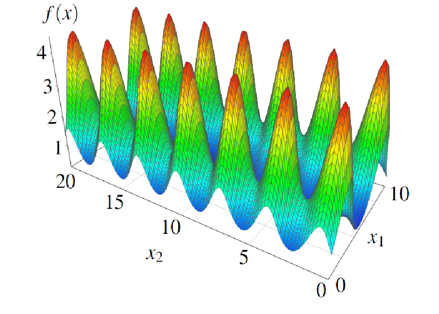The goal of this section is to compare the performance of interval superposition models versus Taylor models on wider domains. Let $f:\mathbb{R}^{2}\to\mathbb{R}$ denote a non-convex factorable function of the form

f(x)=\exp\left(\sin(x_{1})+\sin(x_{2})\cos(x_{2})\right)

on the two-dimensional domain $X=[0,\overline{x}_{1}]\times[0,\overline{x}_{2}]\subseteq\mathbb{R}^{2}$ . Here, $\overline{x}_{1}\geq 0$ and $\overline{x}_{2}\geq 0$ are parameters that can be used to control the diameter of the domain $X$ . The upper left plot in Figure 1 shows a $3$ -dimensional visualization of the function $f$ on the interval domain $[0,10]\times[0,20]$ , i.e., for $\overline{x}_{1}=10$ and $\overline{x}_{2}=20$ . The upper right plot in Figure 1 shows the overestimation of five different enclosure methods for bounding $f$ for $\overline{x}_{1}=10^{-1}$ as a function of the domain parameter $\overline{x}_{2}\in[0.1,20]$ : the red solid and red dotted lines show the overestimation of Taylor models of order $1$ and $2$ , respectively. The black solid, black dotted, and black dashed lines correspond to the overestimation of the enclosures that are obtained by using interval superposition models with $N=1$ , $N=10$ , and $N=100$ . Here, the overestimation is measured in terms of the Hausdorff distance (11) between the exact image set and the five different enclosure sets. The lower left plot in Figure 1 shows the overestimation of the five mentioned methods for a fixed $\overline{x}_{1}=1$ as a function of $\overline{x}_{2}\in[0.1,20]$ . Similarly, the lower right plot in Figure 1 depicts the corresponding results for $\overline{x}_{1}=10$ , again as a function of $\overline{x}_{2}\in[0.1,20]$ . Here, the results for the Taylor models is not shown, as the overestimation error is larger that $10^{7}$ , i.e., Taylor models do not yield reasonable enclosures on this rather large domain. In order to avoid misunderstanding at this point, notice that the width of the exact image set $f(X)$ is monotonically increasing with respect to the parameter $\overline{x}_{2}$ . However, the Hausdorff difference between $f(X)$ and an enclosure $F(X)$ is not necessarily monotonous in $\overline{x}_{2}$ . In fact, also the overestimation of standard Taylor models decreases in sections, if the domain $X$ is increased, although one might argue that, overall, a rough trend is that the overestimation error of the enclosure methods increases when increasing the domain $X$ . One aspect that is not shown in the Figure 1 is that Taylor models do outperform interval superposition models on very small domains, i.e., if we would zoom in and analyze the overestimation for $\overline{x}_{1},\overline{x}_{2}\leq 10^{-1}$ , we could see that Taylor models are the better choice on such small domains. Notice that on the domain $[0,10]\times[0,20]$ the overestimation of the interval superposition method with $N=100$ yields an enclosure that is approximately $1.62$ times larger than the width of the exact range, i.e., the relative over-approximation is approximately $62\;\%$ . This is in contrast to Taylor models, which yield bounds that are more than $10^{7}$ times larger than the exact image set. The performance of Taylor models of order larger than $2$ is not shown in the figure, as they perform even worse than the Taylor models of order $1$ and $2$ on the analyzed, particularly large domains. Here, of course, if we would zoom in on smaller domains $X$ , we could see that increasing the Taylor model order does improve the accuracy for such smaller $X$ [2, 3, 26].

In order to illustrate how the proposed interval superposition arithmetics performs for another, more challenging example, we introduce the function

\displaystyle f_{1}(x)=\left(\begin{array}[]{c}p_{1}\left(e^{-\sin(4x_{1})+x_{2}-x_{2}^{2}-x_{1}^{2}}-1\right)\\[4.55254pt] p_{1}\cos\left(\frac{1}{p_{1}}x_{2}+p_{2}\tan(p_{2}x_{3})\right)-2p_{2}x_{2}^{2}\\[4.55254pt] p_{1}^{2}\sin(\cos(x_{3}))\end{array}\right)\;.

Notice that $f_{1}:\mathbb{R}^{3}\to\mathbb{R}^{3}$ is a multivariate non-convex function with parameters $p_{1}=\frac{1}{10}$ and $p_{2}=\frac{1}{5}$ . In the next step we define the functions

\displaystyle\forall k\in\mathbb{N},\qquad f_{k+1}(x)=f_{1}(f_{k}(x))

(16)

recursively. The goal of this section is to find enclosure sets of the exact image sets $f_{k}(X)$ on the rather large interval domain $X=[-0.25\pi,0.25\pi]\times[-0.5\pi,0.5\pi]^{2}\subseteq\mathbb{R}^{3}$ . The exact image set of the above recursion satisfies a convergence rate condition of the form

\lim_{k\to\infty}\mathrm{diam}\left(f_{k}(X)\right)\;=\;0\;,

i.e., the diameter of the exact image set contracts to $0$ for sufficiently large $k$ .

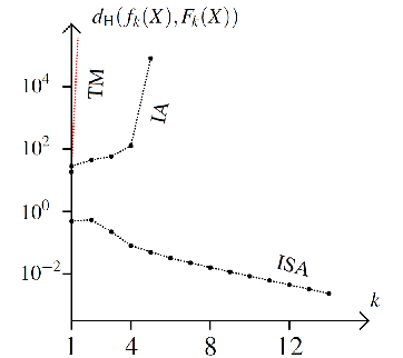
Figure 2 shows the Hausdorff distance between the exact image set $f_{k}(X)$ and the enclosure sets that are obtained by applying standard interval arithmetic, interval superposition arithmetic with $N=20$ , and first order Taylor models with interval remainder bounds. All results are shown in dependence on $k$ . Notice that the interval superposition arithmetic yields convergent enclosure sets that are much less conservative than the enclosures that are obtained by Taylor models and standard interval arithmetic. Taylor models of higher expansion orders perform even worse on this example and are therefore not shown in the figure.

6 Conclusions

This paper has introduced interval superposition arithmetic and illustrated its advantages compared to existing enclosure methods for factorable functions on wider domains. The construction of interval superposition models is based on derivative-free composition rules which exploit global algebraic properties of factorable functions. Interval superposition arithmetic has polynomial run-time and storage complexity of order $\mathbf{O}\left(nN\right)$ , which depends on the number $n$ of variables of the factorable functions and the branching accuracy $N$ . Moreover, this paper has established local and global convergence estimates of the proposed arithmetic. From a practical perspective, the main advantage of interval superposition arithmetics compared to other enclosure methods is that it yields reasonably accurate bounds of the image set of factorable functions on wider interval domains, for which existing methods often yield divergent or very conservative bounds. This advantage has been illustrated through numerical case studies.

Appendix A Derivation of the remainder bounds from Table 1

This section briefly discusses how to derive remainder bounds for interval superposition arithmetic. These remainder bounds are needed in Algorithm 1 and are required to satisfy

\displaystyle\left|\sum_{i=1}^{n}g(\omega+\delta_{i})-(n-1)g(\omega)-g\left(\omega+\sum_{i=1}^{n}\delta_{i}\right)\right|\;\leq\;r_{g}(A)

(17)

for all $\delta\in\mathbb{R}^{n}$ with $\forall i\in\{1,\ldots,n\},\;\;L(A_{i})\leq a_{i}+\delta_{i}\in U(A_{i})$ . Recall that $g\in\mathcal{L}$ denotes a univariate atom function and its associated remainder bound $r_{g}$ depends on the particular properties of $g$ . Also recall that we use shorthand $\omega=\sum_{i=1}^{n}a_{i}$ as introduced in the first step of Algorithm 1.

A.1 Exponential

For the atom function $g(x)=e^{x}$ we have to bound the expression

\displaystyle\sum_{i=1}^{n}g(\omega+\delta_{i})-(n-1)g(\omega)-g\left(\omega+\sum_{i=1}^{n}\delta_{i}\right)

\displaystyle=

\displaystyle e^{\omega}\left[\sum_{i=1}^{n}e^{\delta_{i}}-(n-1)-\prod_{i=1}^{n}e^{\delta_{i}}\right]

for all $\delta_{i}$ with $L(A_{i})\leq a_{i}+\delta_{i}\leq U(A_{i})$ . Let us apply the addition theorem for the exponential function,

e^{\omega+\delta_{i}}=e^{\omega}e^{\delta_{i}}\quad\text{and}\quad e^{\omega+\sum_{i=1}^{n}\delta_{i}}=e^{\omega}\prod_{i=1}^{n}e^{\delta_{i}}\;.

It is convenient to introduce the auxiliary variables $t_{i}=e^{\delta_{i}}-1$ such that

\displaystyle e^{\omega}\left[\sum_{i=1}^{n}e^{\delta_{i}}-(n-1)-\prod_{i=1}^{n}e^{\delta_{i}}\right]

\displaystyle=

\displaystyle e^{\omega}\left[\sum_{i=1}^{n}t_{i}+1-\prod_{i=1}^{n}(1+t_{i})\right]\;.

(18)

The absolute value of this expression can be bounded as

e^{\omega}\left|\sum_{i=1}^{n}t_{i}+1-\prod_{i=1}^{n}(1+t_{i})\right|\;\leq\;e^{\omega}\left(\prod_{i=1}^{n}(1+s_{i})-\sum_{i=1}^{n}s_{i}-1\right)\;

with $s_{i}=\max\left\{e^{\mathrm{U}\left(A_{i}\right)-a_{i}}-1,1-e^{\mathrm{L}\left(A_{i}\right)-a_{i}}\right\}$ . This motivates to choose the central points $a_{i}=\log\left(\frac{1}{2}\left(e^{\mathrm{U}\left(A_{i}\right)}+e^{\mathrm{L}\left(A_{i}\right)}\right)\right)$ such that $s_{i}$ takes the smallest possible value, given by

s_{i}=\frac{e^{\mathrm{U}(A_{i})}-e^{\mathrm{L}\left(A_{i}\right)}}{e^{\mathrm{U}\left(A_{i}\right)}+e^{\mathrm{L}\left(A_{i}\right)}}\;.

In summary, we have shown that

\displaystyle\left|\sum_{i=1}^{n}g(\omega+\delta_{i})-(n-1)g(\omega)-g\left(\omega+\sum_{i=1}^{n}\delta_{i}\right)\right|

\displaystyle\leq

\displaystyle e^{\omega}\left(\prod_{i=1}^{n}(1+s_{i})-\sum_{i=1}^{n}s_{i}-1\right)\;=\;r_{g}(A)\;.

A.2 Inverse

The aim of this section is to find a remainder bound for the atom function $g(x)=\frac{1}{x}$ on the positive domain $\mathbb{R}_{++}=\{x\mid x>0\}$ . Bounds on the domain $\mathbb{R}_{--}=\{x\mid x<0\}$ can be found analogously. If an interval contains $0$ , the bounds are set to $[-\infty,\infty]$ . We start with the equation

		$\displaystyle\sum_{i=1}^{n}g(\omega+\delta_{i})-(n-1)g(\omega)-g\left(\omega+\sum_{i=1}^{n}\delta_{i}\right)=\sum_{i=1}^{n}\frac{1}{\omega+\delta_{i}}-\frac{1}{\omega+\sum_{i=1}^{n}\delta_{i}}-\frac{n-1}{\omega}$
		$\displaystyle\quad=\frac{1}{\omega}\left(\sum_{i=1}^{n}\frac{-\delta_{i}}{\omega+\delta_{i}}+\frac{\sum_{i=1}^{n}\delta_{i}}{\omega+\sum_{i=1}^{n}\delta_{i}}\right)=\frac{1}{\omega}\,\frac{1}{\omega+\sum_{i=1}^{n}\delta_{i}}\,\left(\sum_{i=1}^{n}\frac{\delta_{i}(\delta_{i}-\sum_{k=1}^{n}\delta_{k})}{\omega+\delta_{i}}\right)\;.$

Next, we bound the terms in the last equation separately under the assumption that $\lambda(A)>0$ ,

	$\displaystyle\left\|\frac{1}{\omega+\sum_{i=1}^{n}\delta_{i}}\right\|\leq\frac{1}{\lambda(A)}\;,\quad\left\|\frac{\delta_{i}}{\omega+\delta_{i}}\right\|$	$\displaystyle\leq\max\left\{\,\frac{a_{i}-L(A_{i})}{\omega-a_{i}+L(A_{i})}\,,\,\frac{U(A_{i})-a_{i}}{\omega-a_{i}+U(A_{i})}\,\right\}\;=\;s_{i}\;,$
	$\displaystyle\text{and}\quad\left\|\delta_{i}-\sum_{k=1}^{n}\delta_{k}\right\|$	$\displaystyle\leq\mu(A)-\omega-(U(A_{i})-a_{i})\;.$

Substituting these inequalities yields the desired remainder bound

\left|\sum_{i=1}^{n}g(\omega+\delta_{i})-(n-1)g(\omega)-g\left(\!\omega+\sum_{i=1}^{n}\delta_{i}\!\right)\right|\leq\frac{\sum_{i=1}^{n}s_{i}\left(\mu(A)-\omega-(U(A_{i})-a_{i})\right)}{\omega\lambda(A)}=r_{g}(A).

A.3 Logarithm

The aim of this section is to find a remainder bound for the atom function $g(x)=\log(x)$ on the positive domain $\mathbb{R}_{++}=\{x\mid x>0\}$ ,

		$\displaystyle\sum_{i=1}^{n}g(\omega+\delta_{i})-(n-1)g(\omega)-g\left(\omega+\sum_{i=1}^{n}\delta_{i}\right)$
		$\displaystyle\qquad=\sum_{i=1}^{n}\log\left(\omega+\delta_{i}\right)-\log\left(\omega+\sum_{i=1}^{n}\delta_{i}\right)-(n-1)\log\left(\omega\right)$
		$\displaystyle\qquad=\log\left(\frac{\prod_{i=1}^{n}\left(\omega+\delta_{i}\right)}{\omega^{n-1}\left(\omega+\sum_{i=1}^{n}\delta_{i}\right)}\right)=\log\left(1+\frac{\prod_{i=1}^{n}\left(\omega+\delta_{i}\right)-\omega^{n-1}\left(\omega+\sum_{i=1}^{n}\delta_{i}\right)}{\omega^{n-1}\left(\omega+\sum_{i=1}^{n}\delta_{i}\right)}\right)\;.$

The desired bound is found by bounding the absolute value of this term, choosing the central points $a_{i}=\frac{U(A_{i})+L(A_{i})}{2}$ such that $\left|\delta_{i}\right|\leq s_{i}=\frac{U(A_{i})-L(A_{i})}{2}$ and

		$\displaystyle\left\|\sum_{i=1}^{n}g(\omega+\delta_{i})-(n-1)g(\omega)-g\left(\omega+\sum_{i=1}^{n}\delta_{i}\right)\right\|$
		$\displaystyle\qquad\leq-\log\left(1-\frac{\prod_{i=1}^{n}\left(\omega+s_{i}\right)-\omega^{n-1}\left(\omega+\sum_{i=1}^{n}s_{i}\right)}{\omega^{n-1}\lambda(A)}\right)=r_{g}(A)\;.$

A.4 Sine and Cosine

In order to derive remainder bounds for the sine and cosine functions we use Euler’s formula, $e^{\mathpzc{i}x}=\cos(x)+\mathpzc{i}\sin(x)$ with $\mathpzc{i}=\sqrt{-1}$ . The derivation requires the following steps.

Step 1. In the first step, we derive for all $k\in\{1,\ldots,n\}$ the bound

	$\displaystyle\left\|e^{\pm\mathpzc{i}\delta_{k}}-1\right\|$	$\displaystyle=\left\|\cos(\pm\delta_{k})-1+\mathpzc{i}\sin(\pm\delta_{k})\right\|$
		$\displaystyle=2\left\|\sin\left(\pm\frac{\delta_{k}}{2}\right)\right\|\leq 2\left\|\sin\left(\left[-\frac{U(A_{k})-L(A_{k})}{4},\frac{U(A_{k})-L(A_{k})}{4}\right]\right)\right\|=s_{k}\;.$

Here, the expression for the scalars $s_{k}$ is evaluated by using standard interval arithmetic, i.e.,

	$\displaystyle s_{k}$	$\displaystyle=2\left\|\sin\left(\left[-\frac{U(A_{k})-L(A_{k})}{4},\frac{U(A_{k})-L(A_{k})}{4}\right]\right)\right\|$
		$\displaystyle=\begin{cases}2\sin\left(\frac{U(A_{k})-L(A_{k})}{4}\right)&\text{if}\ \ \frac{U(A_{k})-L(A_{k})}{4}\leq\frac{\pi}{2}\\ 2&\text{otherwise}\end{cases}\;.$

Step 2. In the second step, we use the bounds $s_{k}$ to derive the auxiliary inequalities

\displaystyle\left|\sum_{k=1}^{n}e^{\pm\mathpzc{i}\delta_{k}}-\prod_{k=1}^{n}e^{\pm\mathpzc{i}\delta_{k}}-(n-1)\right|

\displaystyle\leq

\displaystyle\prod_{k=1}^{n}(1+s_{k})-\sum_{k=1}^{n}s_{k}-1\;.

Step 3. The auxiliary inequalities from Step 2 are used to establish the inequalities

		$\displaystyle\left\|\sum_{k=1}^{n}\cos\left(\delta_{k}\right)-\cos\left(\sum_{k=1}^{n}\delta_{k}\right)-(n-1)\right\|$
		$\displaystyle\ =\frac{1}{2}\left\|\sum_{k=1}^{n}e^{\mathpzc{i}\delta_{k}}+\sum_{k=1}^{n}e^{-\mathpzc{i}\delta_{k}}-\prod_{k=1}^{n}e^{\mathpzc{i}\delta_{k}}-\prod_{k=1}^{n}e^{-\mathpzc{i}\delta_{k}}-2(n-1)\right\|\leq\prod_{k=1}^{n}(1+s_{k})-\sum_{k=1}^{n}s_{k}-1$

and, using an analogous argument,

\displaystyle\left|\sum_{k=1}^{n}\sin\left(\delta_{k}\right)-\sin\left(\sum_{k=1}^{n}\delta_{k}\right)\right|\;\leq\;\prod_{k=1}^{n}(1+s_{k})-\sum_{k=1}^{n}s_{k}-1\;.

Step 4. For the sine function, the estimate from Step 3 yields the remainder bound

	$\displaystyle R_{\sin}(\delta)$	$\displaystyle=\left\|\sum_{k=1}^{n}g(\omega+\delta_{k})-(n-1)g(\omega)-g\left(\omega+\sum_{k=1}^{n}\delta_{k}\right)\right\|$
		$\displaystyle=\left\|\sum_{k=1}^{n}\sin\left(\omega+\delta_{k}\right)-\sin\left(\omega+\sum_{k=1}^{n}\delta_{k}\right)-(n-1)\sin\left(\omega\right)\right\|$
		$\displaystyle=\left\|\hphantom{{}+{}}\sin(\omega)\left(\sum_{k=1}^{n}\cos\left(\delta_{k}\right)-\cos\left(\sum_{k=1}^{n}\delta_{k}\right)-(n-1)\right)\right.$
		$\displaystyle\hphantom{{}={}}\,\left.+\cos(\omega)\left(\sum_{k=1}^{n}\sin\left(\delta_{k}\right)-\sin\left(\sum_{k=1}^{n}\delta_{k}\right)\right)\right\|$
		$\displaystyle\leq\left(\|\sin(\omega)\|+\|\cos(\omega)\|\right)\left(\prod_{k=1}^{n}(1+s_{k})-\sum_{k=1}^{n}s_{k}-1\right)=r_{g}(A)\;.$

Similarly, the corresponding bound for the cosine function is given by

$\displaystyle R_{\cos}(\delta)$	$\displaystyle=$	$\displaystyle\left\|\sum_{k=1}^{n}g(\omega+\delta_{k})-(n-1)g(\omega)-g\left(\omega+\sum_{k=1}^{n}\delta_{k}\right)\right\|$
	$\displaystyle=$	$\displaystyle\left\|\sum_{k=1}^{n}\cos\left(\omega+\delta_{k}\right)-\cos\left(\omega+\sum_{k=1}^{n}\delta_{k}\right)-(n-1)\cos\left(\omega\right)\right\|$
	$\displaystyle=$	$\displaystyle\left\|\cos(\omega)\left(\sum_{k=1}^{n}\cos\left(\delta_{k}\right)-\cos\left(\sum_{k=1}^{n}\delta_{k}\right)-(n-1)\right)-\sin(\omega)\left(\sum_{k=1}^{n}\sin\left(\delta_{k}\right)-\sin\left(\sum_{k=1}^{n}\delta_{k}\right)\right)\right\|$
	$\displaystyle\leq$	$\displaystyle\left(\|\sin(\omega)\|+\|\cos(\omega)\|\right)\left(\prod_{k=1}^{n}(1+s_{k})-\sum_{k=1}^{n}s_{k}-1\right)=r_{g}(A)\;.$

A.5 Tangent

In order to construct a remainder bound for the function $g(x)=\tan(x)$ on the open domain $\left(-\frac{\pi}{2},\frac{\pi}{2}\right)$ it is helpful to notice that the addition theorem for this function,

\tan(x+y)=\frac{\tan(x)+\tan(y)}{1-\tan(x)\tan(y)}\;,

can alternatively be written in the difference form

\displaystyle\tan(x+y)-\tan(x)-\tan(y)

\displaystyle=

\displaystyle\tan(x)\tan(y)\tan(x+y)\;.

(19)

The correctness of this equation can be verified by multiplying the addition theorem for the tangent function by $1-\tan(x)\tan(y)$ on both sides and by re-bracketing terms. A generalization of the difference formula (19) for general sums is given by the equation

\displaystyle\rho_{0}(\delta)\;=\;\tan\left(\sum_{i=1}^{n}\delta_{i}\right)-\sum_{i=1}^{n}\tan(\delta_{i})

\displaystyle=

\displaystyle\sum_{i=1}^{n-1}\tan(\delta_{i+1})\tan\left(\sum_{k=1}^{i}\delta_{k}\right)\tan\left(\sum_{k=1}^{i+1}\delta_{k}\right);\,

(20)

which is proven by induction. For $n=2$ , (20) reduces to (19). For the induction step, we have

		$\displaystyle\tan\left(\sum_{i=1}^{n+1}\delta_{i}\right)-\sum_{i=1}^{n+1}\tan(\delta_{i})$
		$\displaystyle\qquad\qquad=\tan\left(\sum_{i=1}^{n+1}\delta_{i}\right)-\tan\left(\sum_{i=1}^{n}\delta_{i}\right)-\tan(\delta_{n+1})+\tan\left(\sum_{i=1}^{n}\delta_{i}\right)-\sum_{i=1}^{n}\tan(\delta_{i})$
		$\displaystyle\qquad\qquad\overset{\eqref{eq::tangentDifference}}{=}\tan\left(\sum_{i=1}^{n+1}\delta_{i}\right)\tan\left(\sum_{i=1}^{n}\delta_{i}\right)\tan(\delta_{n+1})+\left[\tan\left(\sum_{i=1}^{n}\delta_{i}\right)-\sum_{i=1}^{n}\tan(\delta_{i})\right]$
		$\displaystyle\qquad\qquad\overset{\eqref{eq::GenTanDiff}}{=}\sum_{i=1}^{n}\tan(\delta_{i+1})\tan\left(\sum_{k=1}^{i}\delta_{k}\right)\tan\left(\sum_{k=1}^{i+1}\delta_{k}\right)\;.$

Thus, the difference formula (20) holds for all integers $n$ . In order to generalize the above formula further for the case $\omega\neq 0$ , the following algebraic manipulations are made

	$\displaystyle\rho(\delta)$	$\displaystyle=g\left(\omega+\sum_{i=1}^{n}\delta_{i}\right)+(n-1)g(\omega)-\sum_{i=1}^{n}g(\omega+\delta_{i})$
		$\displaystyle=\left[\tan\left(\omega+\sum_{i=1}^{n}\delta_{i}\right)-\tan(\omega)\right]-\sum_{i=1}^{n}\left[\tan(\omega+\delta_{i})-\tan(\omega)\right]$
		$\displaystyle\overset{\eqref{eq::tangentDifference}}{=}\tan\left(\sum_{i=1}^{n}\delta_{i}\right)\left[1+\tan\left(\omega+\sum_{i=1}^{n}\delta_{i}\right)\tan(\omega)\right]-\sum_{i=1}^{n}\tan(\delta_{i})\left[1+\tan(\omega+\delta_{i})\tan(\omega)\right]$
		$\displaystyle=\hphantom{{}+{}}\left(\tan\left(\sum_{i=1}^{n}\delta_{i}\right)-\sum_{i=1}^{n}\tan(\delta_{i})\right)$
		$\displaystyle\hphantom{{}={}}+\tan(\omega)\left(\tan\left(\sum_{i=1}^{n}\delta_{i}\right)\tan\left(\omega+\sum_{i=1}^{n}\delta_{i}\right)-\sum_{i=1}^{n}\tan(\delta_{i})\tan(\omega+\delta_{i})\right)$
		$\displaystyle\overset{\eqref{eq::GenTanDiff}}{=}\rho_{0}(\delta)+\tan(\omega)\left(\hphantom{{}+{}}\rho_{0}(\delta)\tan\left(\omega+\sum_{i=1}^{n}\delta_{i}\right)\right.$
		$\displaystyle\hphantom{{}={}}\kern 76.82234pt+\left.\sum_{i=1}^{n}\tan\left(\delta_{i}\right)\left[\tan\left(\omega+\sum_{i=1}^{n}\delta_{i}\right)-\tan(\omega+\delta_{i})\right]\right)$
		$\displaystyle=\hphantom{{}+{}}\rho_{0}(\delta)\left[1+\tan(\omega)\tan\left(\omega+\sum_{i=1}^{n}\delta_{i}\right)\right]$
		$\displaystyle\hphantom{{}={}}+\sum_{i=1}^{n}\tan(\omega)\tan\left(\delta_{i}\right)\tan\left(\sum_{k\neq i}\delta_{k}\right)\left[1+\tan(\omega+\delta_{i})\tan\left(\sum_{k\neq i}\delta_{k}\right)\tan\left(\omega+\sum_{i=1}^{n}\delta_{i}\right)\right]\;.$

The right-hand expression can be bounded with interval arithmetic yielding

	$\displaystyle\rho(\delta)\leq r_{g}(A)$	$\displaystyle=$	$\displaystyle\left\|\sum_{i=1}^{n-1}\tan(S_{i+1})\tan\left(\sum_{k=1}^{i}S_{k}\right)\tan\left(\sum_{k=1}^{i+1}S_{k}\right)\left[1+\tan(\omega)\tan\left(\omega+\Sigma\right)\right]\right.$
			$\displaystyle\left.+\sum_{i=1}^{n}\tan(\omega)\tan\left(S_{i}\right)\tan\left(T_{i}\right)\left[1+\tan(\omega+S_{i})\tan\left(T_{i}\right)\tan\left(\omega+\Sigma\right)\right]\right\|\;,$

the desired bound. Here we have introduced the auxiliary variables

s_{i}=\frac{U(A_{i})-L(A_{i})}{2}\;,\;\;S_{i}=[-s_{i},s_{i}]\quad\text{and}\quad\sigma=\sum_{i=1}^{n}s_{i}\;,\;\;\Sigma=[-\sigma,\sigma]\;,\;\;T_{i}=[-\sigma+s_{i},\sigma-s_{i}]\;.

Acknowledgments

This research was supported by National Natural Science Foundation China (NSFC), Nr. 61473185, as well as ShanghaiTech University, Grant-Nr. F-0203-14-012.

References

[1] Z. Battles, L.N. Trefethen. An extension of MATLAB to continuous functions and operators. SIAM J. Sci. Comput. 25:1743–1770, 2004.
[2] M. Berz. From Taylor series to Taylor models. In Nonlinear Problems in Accelerator Physics, American Institute of Physics CP405, pp.:1–27, 1997.
[3] M. Berz, G. Hoffstätter. Computation and application of Taylor polynomials with remainder bounds. Reliab. Comput. 4:83–97, 1998.
[4] A. Bompadre, A. Mitsos, B. Chachuat. Convergence analysis of Taylor and McCormick-Taylor models. Journal of Global Optimization 57(1):75–114, 2013.
[5] B. Chachuat, B. Houska, R. Paulen, N. Peric, J. Rajyaguru, M.E. Villanueva. Set theoretic approaches in analysis, estimation and control of nonlinear systems. IFAC-PapersOnLine Volume 48(8), pp:981–995, 2015.
[6] J.P. Eckmann, H. Koch, P. Wittwer. A computer-assisted proof of universality in area-preserving maps. Memoirs of the AMS 47:289, 1984.
[7] L.H. de Figueiredo, J. Stolfi. Affine arithmetic: Concepts and applications. Numerical Algorithms 37(1-4):147–158, 2004.
[8] C.A. Floudas and O. Stein. The Adaptative Convexification Algorithm: a Feasible Point Method for Semi-Infinite Programming. SIAM Journal on Optimization, 18(4):1187–1208, 2007.
[9] C.A. Floudas. Deterministic global optimization: theory, methods and applications. Springer Science & Business Media, Vol. 37, 2013.
[10] B. Houska, M.E. Villanueva, B. Chachuat. Stable Set-Valued Integration of Nonlinear Dynamic Systems using Affine Set Parameterizations. SIAM Journal on Numerical Analysis, 53(5), pp:2307–2328, 2015.
[11] A. Kurzhanski, I. Valyi. Ellipsoidal Calculus for Estimation and Control. Series in Systems & Control: Foundations & Applications, Birkhäuser, 1997.
[12] J.B. Lasserre. Moments, Positive Polynomials and Their Applications. Imperial College Press, 2009.
[13] Q. Lin, J.G. Rokne. Methods for bounding the range of a polynomial. J. Comput Appl Math 58:193–199, 1995.
[14] M. Neher, K.R. Jackson, N.S. Nedialkov. On Taylor model based integration of ODEs. SIAM Journal on Numerical Analysis 45:236–262, 2007.
[15] A. Neumaier. Complete search in continuous global optimization and constraint satisfaction. Acta Numer. 13:271–369, 2004.
[16] K. Makino, M. Berz. Efficient control of the dependency problem based on Taylor model methods. Reliab. Comput. 5(1):3–12, 1999.
[17] G.P. McCormick. Computability of global solutions to factorable nonconvex programs: Part I – Convex underestimating problems. Mathematical Programing 10:147–175, 1976.
[18] R. Misener, C.A. Floudas. GloMIQO: Global Mixed-Integer Quadratic Optimizer. Journal of Global Optimization, 57(1):3–50, 2013.
[19] A. Mitsos, P. Lemonidis, P.I. Barton. Global solution of bilevel programs with a nonconvex inner program. Journal of Global Optimization 42.4:475–513, 2008.
[20] A. Mitsos, B. Chachuat, P.I. Barton. McCormick-based relaxations of algorithms. SIAM Journal on Optimization 20(2):573–601, 2009.
[21] R.E. Moore. Interval Analysis. Prentice-Hall, Englewood Cliffs, NJ, 2966.
[22] R.E. Moore, R.B. Kearfott, M.J. Cloud. Introduction to Interval Analysis. SIAM, Philadelphia, PA, 2009.
[23] J. Rajyaguru, M.E. Villanueva, B. Houksa, B. Chachuat. Higher-Order Inclusions of Factorable Functions by Chebyshev Models. Journal of Global Optimization, Volume 68(2), pp. 413–438, 2017.
[24] H. Ratschek, J. Rokne. Computer Methods for the Range of Functions. Series in Mathematics and Its Applications, Ellis Horwood Ltd, Mathematics and Its Applications, Chichester, UK, 1984.
[25] N.V. Sahinidis. A general purpose global optimization software package. Journal of Global Optimization, 8(2):201–205, 1996.
[26] A.M. Sahlodin, B. Chachuat. Convex/concave relaxations of parametric ODEs using Taylor models. Computers and Chemical Engineering 35(5):844–857, 2011.
[27] M. Tawarmalani, N.V. Sahinidis. A polyhedral branch-and-cut approach to global optimization. Mathematical Programming, 103(2):225–249, 2005.
[28] L.N. Trefethen. Computing numerically with functions instead of numbers. Math. Comput. Sci. 1:9–19, 2007.
[29] A. Townsend, L.N. Trefethen. An extension of Chebfun to two dimensions. SIAM J. Sci. Comput 35(6):C495–C498, 2013.
[30] M.E. Villanueva, J. Rajyaguru, B. Houska, B. Chachuat. Ellipsoidal arithmetic for multivariate systems. Comput. Aided Chem. Eng. 37:767–772, 2015.
[31] M.E. Villanueva, B. Houska, B. Chachuat. Unified Framework for the Propagation of Continuous-Time Enclosures for Parametric Nonlinear ODEs. J. of Global Optim 62(3), pp:575–613, 2015.

	$\displaystyle R_{\sin}(\delta)$	$\displaystyle=\left\|\sum_{k=1}^{n}g(\omega+\delta_{k})-(n-1)g(\omega)-g\left(\omega+\sum_{k=1}^{n}\delta_{k}\right)\right\|$
		$\displaystyle=\left\|\sum_{k=1}^{n}\sin\left(\omega+\delta_{k}\right)-\sin\left(\omega+\sum_{k=1}^{n}\delta_{k}\right)-(n-1)\sin\left(\omega\right)\right\|$
		$\displaystyle=\left\|\hphantom{{}+{}}\sin(\omega)\left(\sum_{k=1}^{n}\cos\left(\delta_{k}\right)-\cos\left(\sum_{k=1}^{n}\delta_{k}\right)-(n-1)\right)\right.$
		$\displaystyle\hphantom{{}={}}\,\left.+\cos(\omega)\left(\sum_{k=1}^{n}\sin\left(\delta_{k}\right)-\sin\left(\sum_{k=1}^{n}\delta_{k}\right)\right)\right\|$
		$\displaystyle\leq\left(\|\sin(\omega)\|+\|\cos(\omega)\|\right)\left(\prod_{k=1}^{n}(1+s_{k})-\sum_{k=1}^{n}s_{k}-1\right)=r_{g}(A)\;.$