Gane Samb LO

Modou NGOM and Tchilabalo A. KPANZOU

Weak Convergence (IA)

Sequences of Random Vectors

Statistics and Probability African Society (SPAS) Books Series.
Calgary, Alberta. 2016.

DOI : http://dx.doi.org/10.16929/sbs/2016.0001

ISBN 978-2-9559183-1-9

SPAS TEXTBOOKS SERIES

GENERAL EDITOR of SPAS EDITIONS

Prof Gane Samb LO
gane-samb.lo@ugb.edu.sn, gslo@ugb.edu.ng
Gaston Berger University (UGB), Saint-Louis, SENEGAL.
African University of Sciences and Technology, AUST, Abuja, Nigeria.

ASSOCIATED EDITORS

KEHINDE DAHUD SHANGODOYIN
shangodoyink@mopipi.ub.bw
UNIVERSITY Of BOTSWANA

Blaise SOME
some@univ-ouaga.bf
Chairman of LANIBIO, UFR/SEA
Ouaga I Pr Joseph Ki-Zerbo University.

ADVISORS

Ahmadou Bamba SOW
ahmadou-bamba.sow@ugb.edu.sn
Gaston Berger University, Senegal.

Tchilabalo Abozou KPANZOU
kpanzout@yahoo.fr
Kara University, Togo.

Library of Congress Cataloging-in-Publication Data

Gane Samb LO, 1958-, Modou NGOM , Tchilabalo A. KPANZOU

Weak Convergence (IA). Sequences of Random Vectors.

SPAS Books Series, 2016.

Statistics and Probability African Society (SPAS).

DOI : 10.16929/sbs/2016.0001

ISBN 978-2-9559183-1-9

Author : Gane Samb LO

Emails:
gane-samb.lo@ugb.edu.sn, ganesamblo@ganesamblo.net.

Url’s:
www.ganesamblo@ganesamblo.net
www.statpas.net/cva.php?email.ganesamblo@yahoo.com.

Affiliations.
Main affiliation : Gaston Berger University, UGB, SENEGAL.
African University of Sciences and Technology, AUST, ABuja, Nigeria.
Affiliated as a researcher to : LSTA, Pierre et Marie Curie University, Paris VI, France.

Teaches or has taught at the graduate level in the following universities:
Saint-Louis, Senegal (UGB)
Banjul, Gambia (TUG)
Bamako, Mali (USTTB)
Ouagadougou - Burkina Faso (UJK)
African Institute of Mathematical Sciences, Mbour, SENEGAL, AIMS.
Franceville, Gabon

Dedicatory.

To my wife Mbaye Ndaw Fall who is accompanying for decades with love and patience

Acknowledgment of Funding.

The author acknowledges continuous support of the World Bank Excellence Center in Mathematics, Computer Sciences and Intelligence Technology, CEA-MITIC. His research projects in 2014, 2015 and 2016 are funded by the University of Gaston Berger in different forms and by CEA-MITIC.

Author : Modou NGOM

Email:
ngomodoungom@gmail.com,ngomodoungom@yahoo.fr

Affiliations.
Main affiliation : Gaston Berger University, UGB, SENEGAL.

Modou Ngom participated in the project of the book while preparing his PhD thesis : On a stochastic process doubly indexed, with margins estimating the extreme value index, and its Gaussian and non Gaussian Asymptotic. He collaborated with Prof Gane Samb LO update this part of his PhD course in Weak convergence to produce the book.

Modou Ngom has also been a lecturer many years in Mathematics, Probability and Measure, at the University of Gaston Berger of Saint-Louis, Senegal,Saint-Louis, Senegal (UGB)

Dedicatory of Modou NGOM.

To my family, whose support, encouragement and faithful prayers arouse my envy to go forward.

Author : Tchilabalo A. KPANZOU

Emails:
kpanzout@gmail.com, kpanzout@yahoo.fr

Url’s:
https://sites.google.com/a/aims.ac.za/tchilabalo
http://univi.net/spas/cvf.php?email=kpanzout@yahoo.fr

Affiliations.
Main affiliation: University of Kara, Kara, TOGO.
Teaches or has taught at the graduate level in the following universities:
University of Kara (UK), TOGO
University of Lomé (UL), TOGO
Ecole Normale Supérieure (ENS), TOGO
University of Abomey-Calavi (UAC), BENIN

Weak Convergence (IA). Sequences of Random Vectors

Abstract.

(English) This monograph aims at presenting the core weak convergence theory for sequences of random vectors with values in $\mathbb{R}^{k}$ . In some places, a more general formulation in metric spaces is provided. It lays out the necessary foundation that paves the way to applications in particular sub-fields of the theory. In particular, the needs of Asymptotic Statistics are addressed. A whole chapter is devoted to weak convergence in $\mathbb{R}$ where specific tools, for example for handling weak convergence of sequences using independent and identically distributed random variables such that the Renyi’s representations by means of standard uniform or exponential random variables, are stated. The functional empirical process is presented as a powerful tool for solving a considerable number of asymptotic problems in Statistics. The text is written in a self-contained approach with the proofs of all used results at the exception of the general Skorohod-Wichura Theorem.

(Français) Cet ouvrage a l’ambition de présenter le noyau dur de la théorie de la convergence vague de suite de vecteurs aléatoires dans $\mathbb{R}^{k}$ . Autant que possible, dans certaines situations, la théorie générale dans des espaces métriques est donnée. Il prépare la voie à une spécialisation dans certains sous-domaines de la convergence vague. En particulier, les besoins de la statistique asymptotique ont été satisfaits. Un chapitre de l’ouvrage concerne la convergence vague dans $\mathbb{R}$ avec des outils spécifiques, par exemple, pour étudier les suites de variables aléatoires indépendantes et identiquement distribuées tels que la représentation de Renyi au moyen de variables aléatoires uniformes ou exponentielles standard. Le processus empirique fonctionnel est introduit comme un outil puissant pour étudier des problèmes asymptotiques en Statistiques. L’ouvrage est rédigé dans une approche auto-citante avec toutes les preuves des résultats utilisés, à l’exception du Théorème de Skorohod-Wichura.

Keywords. Weak convergence; Convergence in distribution; Portmanteau Theorem; Probability Laws characterization; Distribution functions; Characteristic functions; Probability density functions; Random Walks; Empirical processes; Multinomial Laws; Relative compactness; Asymptotic and uniform tightness; Continuous mapping theorem; Renyi and Malmquist representations; Order Statistics; Multivariate Delta methods; Functional empirical process.

AMS 2010 Classification Subjects : 60XXX; 62G30

General Preface

This textbook is the first of series whose ambition is to cover broad part of Probability Theory and Statistics. These textbooks are intended to help learners and readers, of all levels, to train themselves.

As well, they may constitute helpful documents for professors and teachers for both courses and exercises. For more ambitious people, they are only starting points towards more advanced and personalized books. So, these textbooks are kindly put at the disposal of professors and learners.

Our textbooks are classified into categories.

A series of introductory books for beginners. Books of this series are usually accessible to student of first year in universities. They do not require advanced mathematics. Books on elementary probability theory and descriptive statistics are to be put in that category. Books of that kind are usually introductions to more advanced and mathematical versions of the same theory. The first prepare the applications of the second.

A series of books oriented to applications. Students or researchers in very related disciplines such as Health studies, Hydrology, Finance, Economics, etc. may be in need of Probability Theory or Statistics. They are not interested by these disciplines by themselves. Rather, the need to apply their findings as tools to solve their specific problems. So adapted books on Probability Theory and Statistics may be composed to on the applications of such fields. A perfect example concerns the need of mathematical statistics for economists who do not necessarily have a good background in Measure Theory.

A series of specialized books on Probability theory and Statistics of high level. This series begin with a book on Measure Theory, its counterpart of probability theory, and an introductory book on topology. On that basis, we will have, as much as possible, a coherent presentation of branches of Probability theory and Statistics. We will try to have a self-contained, as much as possible, so that anything we need will be in the series.

Finally, research monographs close this architecture. The architecture should be so large and deep that the readers of monographs booklets will find all needed theories and inputs in it.

We conclude by saying that, with only an undergraduate level, the reader will open the door of anything in Probability theory and statistics with Measure Theory and integration. Once this course validated, eventually combined with two solid courses on topology and functional analysis, he will have all the means to get specialized in any branch in these disciplines.

Our collaborators and former students are invited to make live this trend and to develop it so that the center of Saint-Louis becomes or continues to be a reknown mathematical school, especially in Probability Theory and Statistics.

General Preface of Our Series of Weak Convergence

The series Weak convergence is an open project with three categories.

The special series Weak convergence I consists of texts devoted to the core theory of weak convergence, each of them concentrated on the handling of one specific class of objects. The texts will have labels $A$ , $B$ , etc. Here are some examples.

(1) Weak convergence of Random Vectors (IA).

(2) Weak convergence of stochastic processes and empirical processes (IB).

(3) Weak convergence of random measures (IC).

(4) Weak convergence of fuzzy random measures (IC).

The special series Weak convergence II consists of textbooks related to the theory of weak convergence, each of them concentrated on one specialized field using weak convergence. Usually, these subfields are treated apart in the literature. Here, we want to put them in our general frame as continuations of the Weak Convergence Series I. Some examples are the following.

(1) Weak laws of sums of independent random variables.

(2) Weak laws of sums of associated random variables.

(3) Univariate Extreme value Theory.

(4) Multivariate Extreme value Theory.

(5) Etc.

The special series Weak convergence III consists of textbooks focusing on statistical applications of Parts of the Weak Convergence Series I and Weak Convergence Series II. Examples :

(1) A handbook of Gaussian Asymptotic Distribution Using the Functional Empirical Process.

(2) A handbook of Statistical Estimation of the Extreme Value index.

(1) etc.

Preface of The Series Weak Convergence : Sequence of Random Vectors

The series Weak convergence (IA) concerns the theory of weak convergence of sequences of random vectors. Due to the theorem of Kolmgorov, stating broadly that the probability law of any random element is characterized by its finite distribution under the appropriate state spaces, the place of the distributions of random vectors is surely central to Probability Theory.

This motivated us to begin this series by the weak convergence of random vectors as the foundation of all the structure.

Another reason is that the needs of Asymptotic Statistics, which is one of the main motivations of the development of Weak Convergence Theory, generally does not need more than that. This booklet then gives to some readers exactly what they specifically.

This textbook focuses on the study of random elements in $\mathbb{R}^{k}$ , $k\geq 1$ . So the properties and the topology of $\mathbb{R}^{k}$ are used.

But when only the general properties of the metric are used, we prefer to give the results in the general case where the studied sequences have their values in a metric space with a metric $d$ .

The concept of tightness is essential in weak convergence theory. In this text, the Helly-Bray method is exclusively used.

This textbook is concluded by a chapter of the functional empirical process. Here, only the weak limits of its finite distributions are treated. We show how to use it for deriving asymptotic results in many research problems. With such tools, even at this somewhat elementary level of weak convergence, it is possible for readers to provide contributions in many research fields in Statistics and in applied related fields.

I wish you a pleasant reading and hope receiving your feedback.

To my wife Mbaye Ndaw Fall who is accompanying me since decades.

Saint-Louis, Calgary, Abuja, Bamako, Ouagadougou, 2016.

Preliminary Remarks and Notations.

WARNINGS

(1) In all this book, any unspecified limit in presence with the subscripts $n$ are meant as $n\rightarrow+\infty$ .

(2) This textbook deals with general distribution functions $F$ on $\mathbb{R}^{k}$ , $k\geq 1$ . The Lebesgue-Stieljes measure induced by a general distribution function is not necessarily a probability measure. If this induced Lebesgue-Stieljes is a probability measure, we precise this distribution function as a probability distribution function. As well, a distribution function of a random vector $X$ of Lebesgue-Stieljes is implicitly a probability distribution function although we do not say : the probability distribution function of $X$ .

Chapter 1 Review of Usual Weak Convergence Results in $\mathbb{R}^{k}$

1.1. Introduction

In this chapter, we will see that most of the readers, actually know a considerable number of weak convergence results, even if they did not use this concept. What has to be done, on top of this review, is to present these individual results in the frame of a unified theory in the most general setting. This is the target of this book which will be given in the subsequent chapters.

Here, we are going to recall classical convergence results that any student should have encountered from the first courses in probability theory or in Statistics.

We begin to set the general frame of weak convergence in $\mathbb{R}^{k}$ , $k\geq 1$ . We will admit the statements in the following section. We will be able to establish their validity in Chapter 2, in particular in Theorem 3 of that chapter.

1.2. Weak Convergence in $\mathbb{R}^{k}$

Let us remind that the probability law of any vector random variable $X:(\Omega,\mathbb{A},\mathbb{P})\mapsto\mathbb{R}^{k}$ is characterized by

(a) its distribution function:

\mathbb{R}^{k}\ni x\hookrightarrow F_{X}(x)=\mathbb{P}(X\leq x),

(b) its characteristic function (Here, $i$ is the complex number such that $i^{2}=-1$ with positive sinus, and $<.,.>$ stands for the classical product space on $\mathbb{R}^{k}$ )

\mathbb{R}^{k}\ni u\hookrightarrow\Phi(u)=\mathbb{E}(\exp(i<u,X>)),

\mathbb{R}^{k}\ni u\hookrightarrow\Psi_{X}(u)=\mathbb{E}(\exp(<u,X>)).

and

(d) its Radon-Nikodym derivative, or probability density function (pdf), (if it exists), with respect to (w.r.t) a measure $\nu$ on $\mathbb{R}^{k}$ :

d\mathbb{P}/d\nu=f_{X}.

It is interesting that these characteristics also play the main roles in weak convergence through Theorem 3 we will prove in Chapter 2.

We have :

Theorem 1.

(THEOREM-DEFINITION-LEMMA) Let $X_{n}:(\Omega_{n},\mathcal{A}_{n},\mathbb{P}_{n})\mapsto(\mathbb{R}^{k},\mathbb{B}(\mathbb{R}^{k}))$ be a sequence of random vectors, $X:(\Omega_{\infty},\mathcal{A}_{\infty},\mathbb{P}_{\infty})\mapsto(\mathbb{R}^{k},\mathbb{B}(\mathbb{R}^{k}))$ a random vector. Then the assertions (a) and (b) below are equivalent.

(a) For any $u\in\mathbb{R}^{k}$ ,

\Phi_{X_{n}}(u)\rightarrow\Phi_{X}(u)\text{ as }n\rightarrow+\infty.

(b) For any continuity point $u\in\mathbb{R}^{k}$ of $F_{X}$ ,

F_{X_{n}}(x)\rightarrow F_{X}(x)\text{ as }n\rightarrow+\infty.

If one the assertions (a) or (b) holds, we say that the sequence $X_{n}$ weakly converges to $X$ , or $X_{n}$ converges in distributions to $X$ or $X_{n}$ converges in law to $X$ , as $n\rightarrow+\infty$ , and we denote this by

X_{n}\rightsquigarrow X\text{ or }X_{n}\longrightarrow_{d}X\text{ or }X_{n}\overset{\mathcal{L}}{\longrightarrow}X\text{ or }X_{n}\overset{w}{\longrightarrow}X\text{ or }X_{n}\longrightarrow_{w}X

The weak limit is unique in distribution, meaning that if $X_{n}$ weakly converges to $X$ and to $Y$ , then $X$ and $Y$ have the same distribution, that is $F_{X}=F_{Y}$ in the context of $\mathbb{R}^{k}$ .

We also have the following sufficiency weak convergence conditions.

(c) If the moment generating functions (mgf) $\Psi_{X_{n}}$ exist on $B_{n}$ , $n\geq 1$ and $\Psi_{X}$ exists on $B$ , where the $B_{n}$ and $B$ are neighborhoods of $0$ such that $B\subset\cap_{n\geq 0}B_{n}$ , and if for any $x\in B$ ,

\Psi_{X_{n}}(x)\rightarrow\Psi_{X}(x)\text{ as }n\rightarrow+\infty,

then $X_{n}$ weakly converges to $X$ .

(d) Finally, suppose that the probability distribution $\mathbb{P}_{n}(\circ)=\mathbb{P}_{n}(X_{n}\in\circ)$ , $n\geq 1$ , and $\mathbb{P}_{X}(\circ)=\mathbb{P}_{\infty}(X\in\circ)$ have Radon-Nikodym derivatives with respect to a measure $\nu$ on $\mathbb{R}^{k}$ , denoted by

d\mathbb{P}^{n}/d\nu=f_{X_{n}}\ \ n\geq 1,\ \ d\mathbb{P}_{X}/d\nu=f_{X}.

If for any $x\in D_{X}=\{x,f_{X}(x)>0\}$ ,

f_{X_{n}}(x)\rightarrow f_{X}(x)\text{ as }n\rightarrow+\infty,

then $X_{n}\rightsquigarrow X$ .

We have the following last point.

(e) Assume that the sequence $\{X_{n},\ \ n\geq 1\}\subset\mathbb{R}^{k}$ weakly converges to $X\in\mathbb{R}^{k}$ , as $n\rightarrow+\infty$ and let $A$ be a real $(m,k)$ -matrix with $m\geq 1$ . Then $\{AX_{n},\ \ n\geq 1\}\subset\mathbb{R}^{m}$ weakly converges to $AX\in\mathbb{R}^{m}$ .

Remark. Point (e) of Theorem 1 above is a consequence of the continuous mapping Theorem 7 in Chapter 2.

In summary, the weak convergence in $\mathbb{R}^{k}$ holds when the distribution functions, the characteristic functions, the moment generating functions (if they exist) or the probability density functions (if they exist) with respect to the same measure $\nu$ , point-wisely converge to the distribution function, or to the characteristic function or to moment generating function (if it exists), or to the probability density unction (if it exists) with respect to $\nu$ of a probability measure in $\mathbb{R}^{k}$ . In the case of point-wise convergence of the distribution functions, only matters the convergence for continuity points of the limiting distribution functions.

All this is awesome and gives us pretty well tools to deal with weak convergence. The examples given below form the core set of examples you cannot ignore.

But before we proceed to this review, we need a handsome criterion derived from the convergence of characteristic functions.

Proposition 1.

(Wold Criterion). The sequence $\{X_{n},\ \ n\geq 1\}\subset\mathbb{R}^{k}$ weakly converges to $X\in\mathbb{R}^{k}$ , as $n\rightarrow+\infty$ if and only if for any $a\in\mathbb{R}^{k}$ , the sequence $\{<a,X_{n}>,\ \ n\geq 1\}\subset\mathbb{R}$ weakly converges to $<A,X>\in\mathbb{R}$ as $n\rightarrow+\infty$ .

Proof. The proof is quick and uses the notation above. Suppose that $X_{n}$ weakly converges to $X$ in $\mathbb{R}^{k}$ as $n\rightarrow+\infty$ . By using the convergence of characteristic functions, we have for any $u\in\mathbb{R}^{k}$

\mathbb{E}\left(\exp(i<X_{n},u>)\right)\rightarrow\mathbb{E}\left(\exp(i<X,u>)\right)\ \ as\ \ n\rightarrow+\infty.

It follows that for any $a\in\mathbb{R}^{k}$ and for any $t\in\mathbb{R}$ , we have

(1.2.1)

\mathbb{E}\left(\exp(it<X_{n},a>)\right)\rightarrow\mathbb{E}\left(\exp(it<X,a>)\right)\ \ as\ \ n\rightarrow+\infty,

that is, by taking $u=ta$ in the formula above, and by denoting $Z_{n}=<X_{n},a>$ and $Z=<X,a>$ , we have

\mathbb{E}\left(\exp(itZ_{n})\right)\rightarrow\mathbb{E}\left(exp(itZ)\right)\ \ as\ \ n\rightarrow+\infty.

This means that $Z_{n}\rightsquigarrow Z$ , that is $<a,X_{n}>$ weakly converges to $<a,X>$ .

Conversely, suppose that for any $a\in\mathbb{R}^{k}$ , the sequence $\{<a,X_{n}>,\ \ n\geq 1\}\subset\mathbb{R}$ weakly converges to $<A,X>\in\mathbb{R}$ as $n\rightarrow+\infty$ . Then by taking $t=1$ in (2.4.16) we get for any $a=u\in\mathbb{R}^{k}$ ,

\mathbb{E}\left(\exp(i<X,u>)\right)\rightarrow\mathbb{E}\left(\exp(i<X,u>)\right)\ \ as\ \ n\rightarrow+\infty.

which means that $X_{n}\rightsquigarrow X$ as $n\rightarrow+\infty$ .

1.3. Examples of Weak Convergence in $\mathbb{R}$

1.3.1. Weak Convergence of a sequence of Hyper-geometric random variables to a Binomial random variable

Let $X_{N}$ be a random variable following a Hyper-geometric law $\mathcal{H}(N,M,n)$ with $M/N\rightarrow p$ , $N\rightarrow\infty$ , $n$ being fixed. Then $X_{N}$ weakly converges to a Binomial random variable $X$ , that is $X\sim\mathcal{B}(n,p)$ .

Proof. Let us use the probability density functions with respect to the counting measure $\nu$ on $\mathbb{N}$ . We have

f_{X_{n}}(k)=\frac{\left(\begin{tabular}[]{l}$M$\\ $k$\end{tabular}\right)\left(\begin{tabular}[]{l}$N-M$\\ $n-k$\end{tabular}\right)}{\left(\begin{tabular}[]{l}$N$\\ $n$\end{tabular}\right)},0\leq k\leq\min(n,M).

Suppose that $M/N\rightarrow p$ , $N\rightarrow\infty$ . We have

$\displaystyle f_{X_{n}}(k)$	$\displaystyle=$	$\displaystyle\frac{M!}{k!(M-k)!}\frac{(N-M)!}{(n-k)!(N-M-(n-k))!}\frac{n!(N-n)!}{N!}$
	$\displaystyle=$	$\displaystyle\frac{n!}{k!(n-k)!}\times\frac{M!}{(M-k)!}\times\frac{(N-M)!}{(N-M-(n-k))!}\times\frac{(M-n)!}{N!}$
	$\displaystyle=$	$\displaystyle\left(\begin{tabular}[]{l}$n$\\ $k$\end{tabular}\right)\times\left\{\frac{M!}{(M-k)!}\right\}\left\{\frac{(N-M)!}{(N-M-(n-k))!}\right\}\left\{\frac{(M-n)!}{N!}\right\}.$

But

$\displaystyle\left\{\frac{M!}{(M-k)!}\right\}$	$\displaystyle=$	$\displaystyle(M-k+1)(M-k+2)...(M-1)M$
	$\displaystyle=$	$\displaystyle M^{k}(1-\frac{k-1}{M})(1-\frac{k-2}{M})\times...\times(1-\frac{1}{M})$
	$\displaystyle=$	$\displaystyle M^{k}(1+o(1))$

since $M\rightarrow\infty$ and $k$ is fixed. Next,

$\displaystyle\left\{\frac{(N-M)!}{(N-M-(n-k))!}\right\}$	$\displaystyle=$	$\displaystyle(N-M-(n-k)+1)\times...\times(N-M-1)(N-M)$
	$\displaystyle=$	$\displaystyle(N-M)^{n-k}(1+\frac{n-k-1}{N-M})(1+\frac{n-k-2}{N-M})$
	$\displaystyle\times$	$\displaystyle...\times((1+\frac{1}{N-M})$
	$\displaystyle=$	$\displaystyle(N-M)^{n-k}(1+o(1)),$

since, also, $N-M=N(1-M/N)\sim N(1-p)\rightarrow\infty$ and $n-k$ is fixed. Finally

$\displaystyle\left\{\frac{(M-n)!}{N!}\right\}$	$\displaystyle=$	$\displaystyle\frac{1}{(N-n+1)(N-n+2)...(N-1)N}$
	$\displaystyle=$	$\displaystyle\frac{1}{N^{n}(1-\frac{n-1}{N})(1-\frac{n-2}{N})...(1-\frac{1}{N})}$
	$\displaystyle=$	$\displaystyle\frac{1}{N^{n}(1+o(1))}.$

for similar reasons. In total for any $0\leq k\leq n$

f_{X_{n}}(k)=\left(\begin{tabular}[]{l}$n$\\ $k$\end{tabular}\right)\left(\frac{M}{N}\right)^{k}\left(\frac{N-M}{N}\right)^{n-k}(1+o(1))\rightarrow\left(\begin{tabular}[]{l}$n$\\ $k$\end{tabular}\right)p^{k}(1-p)^{n-k}.

Hence, for any $k$ in the support set of the pdf of a $\mathcal{B}(n,p)$ random variable w.r.t to the counting measure $\nu$ , denoted

f_{X}(k)=\left(\begin{tabular}[]{l}$n$\\ $k$\end{tabular}\right)p^{k}(1-p)^{n-k},

we have

\forall(1\leq k\leq n),f_{X_{n}}(k)\rightarrow f_{X}(k).

The proof is finished.

Useful remark in sampling technique theory. This result allows to treat drawing without replacement (which generates a hyper-geometric law) may be approximated as a drawing with replacement (which gives a Binomial law) when the size of the global population is large. The idea behind this is the following : if we randomly draw a small number of individuals from a large set, it is almost improbable that we draw one individual more than one time.

1.3.2. Weak Convergence of a sequence of Binomial random variables to a Poisson random variable

Let $X_{n}$ be a sequence of $\mathcal{B}(n,p)$ random variable with $p=p_{n}\rightarrow 0$ and $np_{n}\rightarrow\lambda$ , $0<\lambda$ , as $n\rightarrow\infty$ . Then $X_{n}$ weakly converges to a Poisson random variable $X$ with parameter $\lambda$ , that is $X\sim\mathcal{\lambda}$ .

Proof. Let us use the moment generating functions. Let $X_{n}$ be a sequence of $\mathcal{B}(n,p_{n})$ -random variable and $X$ be a $\mathcal{P}(\lambda)$ random variable. We have

\Psi_{X_{n}}(t)=((1-p_{n})+p_{n}e^{t})^{n},\text{ }n\geq 1;\Psi_{X}(t)=\exp(\lambda(e^{t}-1)),t\in\mathbb{R}.

Put $\lambda_{n}=np_{n}\rightarrow\lambda$ . For any fixed $t$ , we have

\Psi_{X_{n}}(t)=\left(\frac{\lambda_{n}}{n}+\left(1-\frac{\lambda_{n}}{n}\right)e^{t}\right)^{n}=\left(1-\frac{\lambda_{n}(e^{t}-1)}{n}\right)^{n}\rightarrow\exp(\lambda(e^{t}-1))=\Psi_{X}(t)

by the following classical results of Calculus courses :

\left(1+\frac{x_{n}}{n}\right)^{n}\rightarrow e^{x}\text{ as }n\rightarrow+\infty\text{ whenever }x_{n}\rightarrow x\in\mathbb{R}\text{ as }n\rightarrow+\infty.

1.3.3. Weak Convergence of a sequence of Poisson random variable to a Gaussian random variable

Let $Z_{\lambda}$ be a Poisson random variable with parameter $\lambda>0$ , that is $Z_{\lambda}\sim\mathcal{P}(\lambda)$ . Then the random variable

\frac{Z_{\lambda}-\lambda}{\sqrt{\lambda}}

weakly converges to standard Gaussian random variable $X$ , that is $X\sim\mathcal{N}(0,1)$ , as $\lambda\rightarrow+\infty$ .

Proof. Let us use the moment generating functions. The moment generating function of $Z_{\lambda}\sim\mathcal{P}(\lambda)$ is

\Psi_{Z_{\lambda}}(t)=\exp(\lambda(e^{t}-1)).

Set

Y(\lambda)=\frac{Z_{\lambda}}{\sqrt{\lambda}}=\frac{Z_{\lambda}-\mathbb{E}(X)}{\sigma_{Z_{\lambda}}}.

We have

\Psi_{Y(\lambda)}(u)=e^{-\sqrt{\lambda}}\times\varphi_{Z}(u/\sqrt{\lambda})=e^{-\sqrt{\lambda}}\times\exp(\lambda(e^{u/\sqrt{\lambda}}-1)).

As $\lambda\rightarrow\infty$ , we may use the following expansion

\lambda\left(e^{u/\sqrt{\lambda}}-1\right)=\lambda(1+\frac{u}{\sqrt{\lambda}}+\frac{u^{2}}{2\lambda}+O(\lambda^{-3/2})-1

=u\sqrt{\lambda}+\frac{u^{2}}{2}+O(\lambda^{-1/2}).

Hence

\Psi_{Y(\lambda)}(u)=\exp(\frac{u^{2}}{2}+O(\lambda^{-1/2}))\rightarrow\exp(u^{2}/2).

We conclude that

\frac{Z_{\lambda}}{\sqrt{\lambda}}\rightarrow\mathcal{N}(0,1)

as $\lambda\rightarrow\infty.$

1.3.4. Convergence of a sequence of Binomial random variables to a standard Gaussian random variable

Let $X_{n}$ be a $\mathcal{B}(n,p)$ random variable with $p\in]0,1[$ which is fixed and $n\geq 1$ . Then, as $n\rightarrow\infty$ ,

(1.3.2)

Z_{n}=\frac{X_{n}-np}{\sqrt{npq}}\rightsquigarrow\mathcal{N}(0,1).

Proof. Let us use the moment generating functions. Let $X\sim\mathcal{B}(n,p)$ . We have

\Psi_{X_{n}}(u)=(q+pe^{u})^{n}.

where $q=1-p$ . Then

(1.3.3)

\Psi_{(X_{n}-np)/\sqrt{npq}}(u)=e^{-\sqrt{np/q}}\times\Psi_{X_{n}}(u/\sqrt{npq}),

with

\Psi_{X}(u/\sqrt{npq})=(q+pe^{u/\sqrt{npq}})^{n}.

The idea behind the coming computations is to use a second order expansion of $e^{u/\sqrt{npq}}$ in the neighborhood of $0$ as $n\rightarrow\infty$ and $u$ fixed. We get an expression of the form $1+v_{n}$ , where $v_{n}$ tends to zero. Finally an expansion of the logarithm function $\log(1+v_{n})$ of order 2 is operated.

Hence, as $n\rightarrow\infty$ and $u$ is fixed, we have,

e^{u/\sqrt{npq}}=1+\frac{u}{\sqrt{npq}}+\frac{u^{2}}{2npq}+O(n^{-3/2}).

Next,

(q+pe^{u/\sqrt{npq}})=1+u\sqrt{p/nq}+\frac{u^{2}}{2nq}+O(n^{-3/2})=1+v_{n}

with

v_{n}=u\sqrt{p/nq}+\frac{u^{2}}{2nq}+O(n^{-3/2})\rightarrow 0.

Thus,

$\displaystyle\log\left(1+u\sqrt{p/nq}+\frac{u^{2}}{2nq}+O(n^{-3/2})\right)$	$\displaystyle=$	$\displaystyle\log(1+v_{n})$
	$\displaystyle=$	$\displaystyle v_{n}-\frac{1}{2}v_{n}^{2}+O(v_{n}^{3})$
	$\displaystyle=$	$\displaystyle u\sqrt{p/nq}+\frac{u^{2}}{2nq}-\frac{pu^{2}}{2nq}+O(n^{-3/2}).$

Hence

$\displaystyle\Psi_{X_{n}}(u/\sqrt{npq})$	$\displaystyle=$	$\displaystyle(q+pe^{u/\sqrt{npq}})^{n}=\exp(n\log(q+pe^{u/\sqrt{npq}}))$
	$\displaystyle=$	$\displaystyle\exp\left(n\left(u\sqrt{p/nq}+\frac{u^{2}}{2nq}-\frac{pu^{2}}{2nq}+O(n^{-3/2})\right)\right)$
	$\displaystyle=$	$\displaystyle\exp\left(u\sqrt{np/q}+\frac{u^{2}}{2q}-\frac{pu^{2}}{2q}+O(n^{-1/2})\right)$
	$\displaystyle=$	$\displaystyle e^{u\sqrt{np/q}}e^{u^{2}/2+O(n^{-1/2})}.$

By going back to (1.3.3), we arrive at

\Psi_{(X_{n}-np)/\sqrt{npq}}(u)\rightarrow\exp(u^{2}/2).

This is

(\beta(n,p)-np)/\sqrt{npq}\rightarrow_{w}\mathcal{N}(0,1)\ \ as\ \ n\rightarrow+\infty.

QED.

Remark. We will come back for a direct proof of this result using the central limit theorem stated just below.

1.3.5. Convergence of a sequence of Negative Binomial random variables to a standard Gaussian random variable

Let $Y_{k}$ be a sequence of $\mathcal{NB}(k,p)$ random variable with $p\in]0,1[$ which is fixed and $k\geq 1$ . Then, as $k\rightarrow\infty$ ,

(1.3.4)

Z_{k}=\frac{p(Y_{k}-\frac{k}{p})}{\sqrt{qk}}\rightsquigarrow\mathcal{N}(0,1).

Proof. Let $t\in\mathbb{R}$ fixed. We write

Z_{k}=\frac{p}{\sqrt{kq}}Y_{k}-\sqrt{\frac{k}{q}}

and remind that

\varphi_{Y_{k}}(t)=\left(\frac{pe^{t}}{1-qe^{t}}\right)^{k}.

$\displaystyle\varphi_{Z_{k}}(t)$	$\displaystyle=$	$\displaystyle\exp(-t\sqrt{\frac{k}{q}})\varphi_{Y_{k}}\left(\frac{pt}{\sqrt{kq}}\right)$
	$\displaystyle=$	$\displaystyle\exp\left(-t\sqrt{\frac{k}{q}}\right)\left(\frac{p\exp(\frac{pt}{\sqrt{kq}})}{1-q\exp(\frac{pt}{\sqrt{kq}})}\right)^{k}$
	$\displaystyle=$	$\displaystyle\exp\left(-t\sqrt{\frac{k}{q}}\right)\exp\left(k\log\left(\frac{p\exp(\frac{pt}{\sqrt{kq}})}{1-q\exp(\frac{pt}{\sqrt{kq}})}\right)\right)$
	$\displaystyle=:$	$\displaystyle\exp\left(-t\sqrt{\frac{k}{q}}\right)\exp(k\log(B_{k}))$

with

	$\displaystyle B_{k}$	$\displaystyle=:$	$\displaystyle\frac{p\exp(\frac{pt}{\sqrt{kq}})}{1-q\exp(\frac{pt}{\sqrt{kq}})}$
		$\displaystyle=:$	$\displaystyle\frac{B_{k,1}}{B_{k,2}}.$

Now, since $pt/\sqrt{kq}\rightarrow 0$ as $k\rightarrow+\infty$ , we get the second order expansions of $B_{k,1}$ and $B_{k,1}$ as follows :

B_{k,1}=p\left(1+\frac{pt}{\sqrt{kq}}+\frac{p^{2}t^{2}}{2kq}+O(k^{\frac{-3}{2}})\right)

and

B_{k,2}=1-q\left(\frac{pt}{\sqrt{kq}}+\frac{p^{2}t^{2}}{2kq}+O(k^{\frac{-3}{2}})\right)=p\left(1-t\sqrt{\frac{q}{k}}-\frac{pt^{2}}{2k}+O(k^{\frac{-3}{2}})\right)

It comes that

$\displaystyle B_{k}$	$\displaystyle=$	$\displaystyle\frac{B_{k,1}}{B_{k,2}}$
	$\displaystyle=$	$\displaystyle\frac{p\left(1+\frac{pt}{\sqrt{kq}}+\frac{p^{2}t^{2}}{2kq}+O(k^{\frac{-3}{2}})\right)}{p\left(1-t\sqrt{\frac{q}{k}}-\frac{pt^{2}}{2k}+O(k^{\frac{-3}{2}})\right)}$
	$\displaystyle=:$	$\displaystyle\frac{1+a_{k}}{1-b_{k}},$

with

\log(1+a_{k})=a_{k}-\frac{1}{2}a_{k}^{2}+O(a_{k}^{3})

and

\log(1-b_{k})=-b_{k}-\frac{1}{2}b_{k}^{2}+O(b_{k}^{3}).

Hence, we get

\displaystyle\log(B_{k})

\displaystyle=

\displaystyle\frac{pt}{\sqrt{kq}}+t\sqrt{\frac{k}{q}}+\frac{t^{2}}{2k}+O(k^{\frac{-3}{2}}).

Next, we have

$\displaystyle\exp\left(k\log(B_{k})\right)$	$\displaystyle=$	$\displaystyle\exp\left(pt\sqrt{\frac{k}{q}}+t\sqrt{kq}+\frac{t^{2}}{2}+O(k^{\frac{-1}{2}})\right)$
	$\displaystyle=$	$\displaystyle\exp\left((1-q)t\sqrt{\frac{k}{q}}+t\sqrt{kq}+\frac{t^{2}}{2}+O(k^{\frac{-1}{2}})\right)$
	$\displaystyle=$	$\displaystyle\exp\left(t\sqrt{\frac{k}{q}}+\frac{t^{2}}{2}+O(k^{\frac{-1}{2}})\right).$

Finally, we get

$\displaystyle\varphi_{Z_{k}}(t)$	$\displaystyle=$	$\displaystyle\exp\left(-t\sqrt{\frac{k}{q}}\right)\exp\left(t\sqrt{\frac{k}{q}}+\frac{t^{2}}{2}+O(k^{\frac{-1}{2}})\right)$
	$\displaystyle=$	$\displaystyle\exp\left(\frac{t^{2}}{2}+O\left(k^{-1/2}\right)\right)$
	$\displaystyle\rightarrow$	$\displaystyle\varphi_{\mathcal{N}(0,1)}(t)\ as\ k\rightarrow+\infty.\ \square$

1.3.6. Simple Central Limit Theorem in $\mathbb{R}$ .

The two last cases are special cases of a more general weak convergence theorem, called the central limit theorem (CLT) of Probability Theory. We say that a sequence of real random variables $(X_{n})_{n\geq 1}$ , for which each $X_{n}$ has a positive finite second moment, satisfies the CTL property if and only if

\frac{X_{n}-E(X_{n})}{\sigma_{X_{n}}}

weakly converges to Gaussian standard random variable. This, of course, is not always true. Here, we will see a simple case. Later, we will give a global solution of this problem in $\mathbb{R}$ .

Let $X_{1},X_{2},...$ be a sequence of real valued random variables which are independent and identically distributed (iid) random variables with common distribution function $F$ with

E(X_{i})=\mu=\int xdF(x)=0,\sigma_{X_{i}}^{2}=\sigma^{2}=\int(x-\mu)^{2}dF(x)=1.

Put, for $n\geq 1$ ,

S_{n}=X_{1}+...+X_{n}.

We have, as $n\rightarrow\infty$ ,

\frac{S_{n}}{\sqrt{n}}\rightarrow\mathcal{N}(0,1).

Proof. Consider the common characteristic function

\mathbb{R}\ni u\hookrightarrow\Phi_{X_{i}}(u)=E(e^{iuX_{i}})=\Psi(u).

Since the second moment exists, we have the following expansion at order 2,

\Phi(u)=1+iu\Phi^{\prime}(0)+\frac{1}{2}u^{2}\Phi^{\prime\prime}(0)+O(u^{3})

=1-\frac{1}{2}u^{2}+O(u^{2})

since

\Phi^{\prime}(0)=i\text{ }\mathbb{E}(X)=0,\text{ }\Phi^{\prime\prime}(0)=-\mathbb{E}(X^{2})=-1.

Thus

\Phi_{S_{n}/\sqrt{n}}(u)=(\Phi(u/\sqrt{n}))^{n}.

For $u$ fixed, as $n\rightarrow\infty$ ,

$\displaystyle\Phi_{S_{n}/\sqrt{n}}(u)$	$\displaystyle=$	$\displaystyle(\Phi(u/\sqrt{n}))^{n}=\exp\left(n\log(1-\frac{u^{2}}{2n}+O(n^{-3/2}))\right)$
	$\displaystyle=$	$\displaystyle\exp(n(-\frac{u^{2}}{n}+O(n^{-3/2}))$
	$\displaystyle=$	$\displaystyle\exp(-u^{2}/2+O(n^{-1/2}))$
	$\displaystyle\rightarrow$	$\displaystyle\exp(-u^{2}/2).$

We just established

\frac{S_{n}}{\sqrt{n}}\rightarrow\mathcal{N}(0,1)\ \ as\ n\rightarrow+\infty.

In a more general case of an iid sequence of random variables $X_{1}$ , $X_{2}$ , … with

\mathbb{E}(X_{i})=\mu=\int xdF(x)=\mu,\sigma_{X_{i}}^{2}=\sigma^{2}=\int(x-\mu)^{2}dF(x)=\sigma^{2},

we apply the former result to the sequence $(X_{i}-\mu)/\sigma$ , $i=1,2,...$ to get

\frac{1}{\sigma\sqrt{n}}(S_{n}-n\mu)\rightarrow\mathcal{N}(0,1).

Let us give two examples of applications of the simple central limit theorem on the binomial trials.

Example 1 : Weak convergence of the binomial random variable.

We are going to prove the result (1.3.2) of Subsetion 1.3.4 concerning the weak law of a sequence of binomial random variables as the number of trials, $n$ , increases while the probability of success, $p\in]0,1[$ , is fixed. So we keep the notation of that subsection.

We know from the earlier courses on elementary Probability Theory we may find in a considerable number of books, especially in [6], with the current Probability Theory and Statistics Series, in Chapter 2, Lemma 1, that if $X_{n}\sim\mathcal{B}(n,p)$ , then $X_{n}$ is the sum of $n$ independent Bernoulli $\mathcal{B}(p)$ random variables $Y_{1},...,Y_{n}$ such that

X_{n}=Y_{1}+...+Y_{n}.

For each of the $Y_{i}$ ’s random variables, we have

\mathbb{E}(Y_{i})=p\text{ and }\sigma^{2}=\mathbb{V}ar(Y_{i})=pq\text{ where }q=1-p.

Then, the random variable $Z_{n}$ in Formula (1.3.2) becomes

Z_{n}=\frac{X_{n}-np}{\sqrt{npq}}=\frac{1}{\sigma\sqrt{n}}\sum_{i=1}^{n}(Y_{i}-\mathbb{E}(Y_{i})).

Hence, the weak convergence of $Z_{n}$ to $\mathcal{N}(0,1)$ as $n\rightarrow+\infty$ , is a consequence of the simple central limit standard on $\mathbb{R}$ .

Remark. This proof is quick and beautiful. The first proof is still useful. Because, we may be in a position to teach this result at a level where the central limit theorem is not available. Besides, this proof is part of History. In the same spirit, the oldest proof of this result goes back to 1732 by de Moivre and to 1801 by Laplace (see Loève [10], page 23). These historical methods can also be found in [6] and in [7] with a writing which is appropriate to beginners of first year of university.

Example 2 : Negative Binomial Law.

For a fixed integer $k\geq 1$ , a Negative Binomial random variable $X_{k}$ is defined relatively to Bernoulli trails of probability of success $p\in]0,1[$ . The number of repetitions of a Bernoulli experiment of parameter $p$ which is necessary to obtain $k$ successes is said to follow a Negative Binomial random variable with parameters $k$ and $p$ , denoted by $X_{k}\sim\mathcal{NB}(k,p)$ . For $k=1$ , it is said that $X_{1}$ follows a geometric law with parameter $p$ , denoted $X_{1}\sim\mathcal{G}(p)$ .

Similarly to the sequence of binomial random variable, we may apply the central limit theorem to the sequence of negative binomial random variables $X_{k}$ , $k\geq 1$ to get the following result

(1.3.5)

Z_{n}=\frac{p(X_{k}-\frac{k}{p})}{\sqrt{nq}}\rightsquigarrow\mathcal{N}(0,1)\text{ as }k\rightarrow+\infty.

To this purpose, the reader may find more details in classical elementary books in probability theory, for instance in [6] or in [7], Chapters 2 and 3. In Chapter 2 of these monographs, Lemma 2, ensures that a $\mathcal{NB}(k,p)$ random variables $X_{k}$ is the sum of $k$ independent and geometric $\mathcal{G}(p)$ random variables $Y_{1},...,Y_{k}$ such that

X_{k}=Y_{1}+...+Y_{n},

and for each of these random variables $Z_{i}$ ’s, we have

\mathbb{E}(Y_{i})=\frac{1}{p}\text{ and }\sigma^{2}=\mathbb{V}ar(Y_{i})=\frac{q}{p^{2}}\text{ where }q=1-p.

Thus, by the central limit theorem

Z_{n}=\frac{p(X_{k}-\frac{k}{p})}{\sqrt{nq}}=\frac{1}{\sigma\sqrt{n}}\sum_{i=1}^{n}(Y_{i}-\mathbb{E}(Y_{i}))\rightsquigarrow\mathcal{N}(0,1)\text{ as }k\rightarrow+\infty.

which proves (1.3.5).

1.3.7. Limit laws in Extreme value Theory

Consider $X_{1},X_{2}$ , … a sequence of iid random variables with common distribution function $F$ . Put for each $n\geq 1$ ,

M_{n}=\max(X_{1},...,X_{n}).

Recall that for any $x\in\mathbb{R}$

P(M_{n}\leq x)=F(x)^{n},x\in\mathbb{R}.

The basic problem of extreme value theory is finding sequences $\left(a_{n}>0\right)_{n\geq 1}$ and $\left(b_{n}\right)_{n\geq 1}$ such that

\frac{M_{n}-b_{n}}{a_{n}}

weakly converges to some random variable $Z$ ,

\frac{M_{n}-b_{n}}{a_{n}}\rightsquigarrow Z.

If this holds, we write $F\in D(F_{Z})$ .

We are going to give three examples corresponding to the three nontrivial cases.

(a) Let $\Lambda$ be a Gumbel random variable of distribution function

\Lambda(x)=exp(-e^{-x}),\ \ x\in\mathbb{R}.

Let the $X_{i}$ ’s are standard exponential random variables, $X_{i}\sim\mathcal{E}(1)$ , with

F(x)=(1-\exp(-x))1_{(x\geq 0)},\text{ }x\in\mathbb{R}.

We have, as $n\rightarrow+\infty$ ,

(1.3.6)

M_{n}-\log n\rightsquigarrow\Lambda.

Proof. By using the distribution functions, we want to prove that for any $x\in\mathbb{R}$ ,

(1.3.7)

\mathbb{P}(M_{n}-\log n\leq x)\rightarrow\Lambda(x).

Proof. We are going to show, by using the distribution functions, that

Indeed, we have

\mathbb{P}(M_{n}-\log n\leq x)=P(M_{n}\leq x+\log n)=F(x+\log n)^{n}.

But for any $x\in\mathbb{R},$ $x+\log n\geq 0$ for $n\geq\exp(-x).$ Then for large values of $n$ , $P(M_{n}\leq x+\log n)=(1-\exp(-x-\log n))^{n}$ and next for any $x\in\mathbb{R}$ and for $n$ large enough,

\mathbb{P}(M_{n}-\log n\leq x)=\left(1-\frac{e^{-x}}{n}\right)\rightarrow e^{-e^{-x}}=\Lambda(x).

So (1.3.7) holds and so does (1.3.6), that is : $X\in D(\Lambda)$ .

(b) Let $FR(\alpha)$ a Fréchet random variable with parameter $\alpha>0$ , with distribution function

\phi_{\alpha}(x)=exp(-x^{-\alpha})1_{(x\geq 0)},

where $1_{A}$ is the indicator function of the set $A$ that assigns the value one to elements of $A$ and zero to elements of the complementary of $A$ .

Let the $X_{i}$ ’s be Pareto random variables with parameter $\alpha>0$ , $X\sim\mathcal{P}ar(\alpha)$ , with common distribution function

F(x)=(1-x^{-\alpha})\ 1_{(x\geq 1)},\text{ }x\in\mathbb{R}

Then, as $n\rightarrow+\infty$ , we have

(1.3.8)

n^{-1/\alpha}M_{n}\rightsquigarrow FR(\alpha).()

Proof. We want to prove that for any $x\in\mathbb{R}$ , we have as $n\rightarrow+\infty$ ,

(1.3.9)

\mathbb{P}(n^{-1/\alpha}M_{n}\leq x)\rightarrow\phi_{\alpha}(x).

The observations $X_{i}$ ’s are non-negative since the support of a $\mathcal{P}ar(\alpha)$ law is $\mathbb{R}_{+}$ . So the maxima $M_{n}$ are non-negative for any $n\geq 1$ . We may discuss two cases.

Case $x\leq 0$ . In this case, we have

\mathbb{P}(n^{-1/\alpha}M_{n}\leq 0)=0=\phi_{\alpha}(x),

and then (1.3.9) holds.

Case $x>0$ . In this case

P(n^{-1/\alpha}M_{n}\leq x)=P(M_{n}\leq n^{1/\alpha}x).

For large values of $n$ , we have $n^{1/\alpha}x>1$ (take $n\geq x^{-\alpha}$ , to ensure that) and for these values,

	$\displaystyle\mathbb{P}(n^{-1/\alpha}M_{n}$	$\displaystyle\leq$	$\displaystyle x)=F(n^{1/\alpha}x)^{n}=(1-(n^{1/\alpha}x)^{-\alpha})^{n}$
		$\displaystyle=$	$\displaystyle\left(1-\frac{x^{-\alpha}}{n}\right)^{n}\rightarrow\exp(-x^{-\alpha})=\phi_{\alpha}(x).$

So (1.3.9) holds for $x>0$ . But putting together the two cases, we have $F\in D(FR(\alpha))$ .

\psi_{\alpha}(x)=exp(-(-x)^{\beta})1_{x\leq 0}+1_{(x>0)}.

Let the $X_{i}$ ’s be uniformly distributed on $(0,1)$ with probability distribution function :

F(x)=x1_{(0\leq x\leq 1)}+1_{(x\geq 1)},\text{ }x\in\mathbb{R}.

We have

(1.3.10)

n(M_{n}-1)\overset{d}{\rightarrow}W(1)\text{ as }n\rightarrow+\infty.

Proof. We have to prove that for any $x\in\mathbb{R}$ , as $n\rightarrow+\infty$ ,

(1.3.11)

\mathbb{P}(n(M_{n}-1)\leq x)=F\left(1+\frac{x}{n}\right)^{n}\rightarrow\psi_{1}(x).

We have two cases.

Case $x\geq 0$ . We see that $1+x/n$ is non-negative for $n\geq 1$ and

P(n(M_{n}-1)\leq x)=F(1+\frac{x}{n})^{n}=1=\psi_{1}(x)

and we see that (1.3.11) holds for $x\geq 0$ .

Case $x<0$ . For large values of $n$ , we have $0\leq 1+x/n\leq 1$ (take $0\geq-x\geq n$ , to get it) and for these values of $n$ ,

	$\displaystyle P(n(M_{n}-1)$	$\displaystyle\leq$	$\displaystyle x)=F\left(1+\frac{x}{n}\right)^{n}$
		$\displaystyle=$	$\displaystyle\left(1+\frac{x}{n}\right)^{n}\rightarrow e^{x}=\psi_{1}(x).$

Then (1.3.11) also holds for $x<0$ and then (1.3.11) holds for any $x\in\mathbb{R}$ ,

\mathbb{P}(n(M_{n}-1)\leq x)\longrightarrow\psi_{1}(x).

Conclusion : $F\in D(W(1))$ .

Summary. In Uni-variate Extreme Value Theory (UEVT), it is proved that the three non-degenerated possible limits are the three we gave above. You will have the opportunity to go deep in that theory in the book of this series [5].

1.4. Examples of Convergence in $\mathbb{R}^{k}$

1.4.1. Simple Central Limit in $\mathbb{R}^{k}$

We now move to the Central Limit Theorem in $\mathbb{R}^{k}$ in the iid case. Let $X_{1},X_{2},....$ be centered iid $\mathbb{R}^{k}$ -random variables with common finite variance-covariance matrix $\Sigma=(\sigma_{ij})_{1\leq i\leq k,1\leq j\leq k}$ , that is

\sigma_{ij}=Cov(X_{i},X_{j})\in\mathbb{R},\ \ 1\leq i,j\leq k.

Set the partial sums

S_{n}=X_{1}+X_{2}+...+X_{n},\ \ n\geq 1.

We have the following central limit theorem on $\mathbb{R}^{k}$ ,

S_{n}/\sqrt{n}\rightsquigarrow\mathcal{N}(0,\Sigma)\ \ as\ \ n\rightarrow+\infty.

Proof. The matrix $\Sigma$ is symmetrical and non-negative in the sense that for any $u\in\mathbb{R}^{k}$

\text{ }^{t}u\Sigma u=\text{ }^{t}u\mathbb{E}(XX^{\prime})u=\mathbb{E}((\text{ }^{t}Xu)(\text{ }^{t}Xu))=\mathbb{E}((\text{ }^{t}Xu)^{2})\geq 0.

By the matrices theory, $\Sigma$ has $k$ non-negative eigenvalues $\lambda_{1}$ , $\lambda_{2}$ ,…, $\lambda_{k}$ and there exists a orthogonal $(k,k)$ -matrix $T$ such that

\text{ }^{t}T\Sigma T=diag(\lambda_{1},\lambda_{2},...,\lambda_{n})=\Lambda.

Set

Y_{i}=\text{ }^{t}TX_{i}.

The random variables $Y_{i}$ are centered, iid and have common variance-covariance matrix equal to

\Sigma_{Y}=\text{ }^{t}T\Sigma T=\Lambda.

This means that the components of each $Y_{i}$ are uncorrelated and have variances equal to $\lambda_{1},\lambda_{2},...,\lambda_{n}$ . Set

(1.4.1)

M_{n}=\frac{1}{\sqrt{n}}(Y_{1}+Y_{2}+...+Y_{n})=\text{ }^{t}T\left(\frac{S_{n}}{\sqrt{n}}\right).

For any $A=\text{ }^{t}(a_{1},a_{2},...,a_{k})\in\mathbb{R}^{k}$ ,

<A,M_{n}>=\frac{1}{\sqrt{n}}\sum_{i=1}^{n}<A,Y_{i}>.

The variables $<A,Y_{i}>$ then are iid and have common variance

\mathbb{E}<A,Y_{i}>^{2}=\sum_{i=1}^{n}a_{i}^{2}\lambda_{i}=\text{ }^{t}A\Lambda A,

because of the mack of correlation between the components of each $Y_{i}$ . We may apply the central limit theorem in $\mathbb{R}$ to get

<A,M_{n}>\rightarrow\mathcal{N}(0,\sum_{i=1}^{i=n}a_{i}^{2}\lambda_{i})=\mathcal{N}(0,\text{ }^{t}A\Lambda A)

But $\mathcal{N}(0,\text{ }^{t}A\Lambda A)$ is the law of a Gaussian random variable that is the linear transform $\text{ }^{t}AZ=<A,Z>$ of $Z$ , where $Z$ follows the $\mathcal{N}(0,\Lambda)$ law. Then

\forall A\in\mathbb{R}^{k},<A,M_{n}>\rightsquigarrow<A,Z>.

In terms of characteristic functions, we have for any $t\in\mathbb{R}$ and for any $A\in\mathbb{R}^{k}$ ,

\mathbb{E}\exp(it<A,M_{n}>)\rightarrow\mathbb{E}\exp(it<A,Z>).

For $t=1$ , we have for any $A\in\mathbb{R}^{k}$

\Phi_{M_{n}}(A)=\mathbb{E}\exp(i<A,M_{n}>)\rightarrow\Phi_{Z}(A)=\mathbb{E}\exp(i<A,Z>).

This means that

M_{n}\rightsquigarrow Z.

This, Point (e) of Theorem 1 and (1.4.1) together implies that

S_{n}/\sqrt{n}=TM_{n}\rightsquigarrow TZ

and then

\text{ }^{t}TZ\sim\mathcal{N}(0,T\Lambda\text{ }^{t}T)=\mathcal{N}(0,\Sigma).

Hence, finally, as $n\rightarrow+\infty$ ,

S_{n}/\sqrt{n}\rightsquigarrow\mathcal{N}(0,\Sigma).

1.4.2. Weak Convergence of the Multinomial Law

A $k$ -tuple $X_{n}=(X_{1,n},...,X_{k,n})$ follows a multinomial law with parameters $n\geq 1$ and $p=(p_{1},p_{2},...,p_{k})$ , with

\forall(1\leq i\leq k),p_{i}>0\text{ \ }and\text{ \ }\sum_{1\leq i\leq k}p_{i}=1,

denoted $X\sim\mathcal{M}_{k}(n,p)$ , if and only if its probability law is given by

\mathbb{P}(X_{1,n}=n_{1},...,X_{k,n}=n_{k})=\frac{n!}{n_{1}!\times...\times n_{k}!}p_{1}^{n_{1}}\times p_{2}^{n_{2}}\times...\times p_{k}^{n_{k}},

where $(n_{1},...,n_{k})$ satisfies

\forall(1\leq i\leq k),\text{ }n_{i}\geq 0\text{ \ et \ }\sum_{1\leq i\leq k}n_{i}=n.

A random variable following the $\mathcal{M}_{k}(n,p)$ law may be generated as follows :

Consider a random experiment with $k$ possible outcomes $E_{i},1$ $\leq i\leq k$ , each of them occurring with $p_{i}>0$ . After $n$ repetitions, the number of occurrences $X_{i,n}$ of each $E_{i}$ is observed for $i=1,...,k$ . The resulting random vector follows the $\mathcal{M}_{k}(n,p)$ law. Each individual coordinate $X_{i,n}$ follows the Binomial law $\mathcal{B}(n,p_{i})$ .

We have the following weak convergence result.

Put

(1.4.2)

Z_{n}=\text{ }^{t}\left(\frac{X_{1,n}-np_{1}}{\sqrt{np_{1}}},...,\frac{X_{k,n}-np_{k}}{\sqrt{np_{k}}}\right)\rightsquigarrow\mathcal{N}_{k}(0,\Sigma)\ \ as\ \ n\rightarrow+\infty,

where $\Sigma$ is a $(k,k)$ -matrix with elements $\Sigma_{i,i}=1-p_{i}$ and $\Sigma_{i,j}=-\sqrt{p_{i}p_{j}}$ , $1\leq i,j\leq k$ .

Important remark. This result has a significant number of applications. We may cite two of them. It is used to have the finite-distribution function of the empirical process. It also serves as the foundations of Chi-square statistical tests that will be studied latter in one the books of this series.

Proof. We have at least two ways of proving the result. The first is based on the use of the moment generating function on logarithm expansions. The second exploits the central limit theorem in $\mathbb{R}^{k}$ we just proved.

First proof. We already know from [9] that its moment generating function is

\phi_{X_{n}}(u)=\left(\sum_{1\leq i\leq k}p_{i}e^{u_{i}}\right)^{n}.

We have

Z_{n}=AX+B,

where $A$ is the diagonal matrix

A=diag\left(\frac{1}{\sqrt{np_{1}}},\frac{1}{\sqrt{np_{2}}},...,\frac{1}{\sqrt{np_{k}}}\right)

and

B=\left(\begin{array}[]{c}-\sqrt{np_{1}}\\ -\sqrt{np_{2}}\\ ...\\ -\sqrt{np_{k}}\end{array}\right).

Thus

	$\displaystyle\phi_{Z_{n}}(u)$	$\displaystyle=$	$\displaystyle\exp(<B,u>)\times\phi_{X}(\text{ }^{t}Au)$
		$\displaystyle=$	$\displaystyle\left(\exp\left(\sum_{1\leq i\leq k}-\sqrt{np_{i}}u_{i}\right)\right)\times\left(\sum_{1\leq i\leq k}p_{i}e^{u_{i}/\sqrt{np_{i}}}\right)^{n}.$

Let $u$ be fixed. For each fixed $i$ , $1\leq i\leq k$ , $u_{i}/\sqrt{np_{i}}\rightarrow+\infty$ as $n\rightarrow\infty$ since $p_{i}>0$ . We have the expansion

e^{u_{i}/\sqrt{np_{i}}}=1+u_{i}/\sqrt{np_{i}}+\frac{1}{2}\frac{u_{i}^{2}}{np_{i}}+O(n^{-3/2}).

	$\displaystyle A$	$\displaystyle=$	$\displaystyle\left(\sum_{1\leq i\leq k}p_{i}e^{u_{i}/\sqrt{np_{i}}}\right)^{n}=\exp\left(n\log\left(\sum_{1\leq i\leq k}p_{i}e^{u_{i}/\sqrt{np_{i}}}\right)\right).$
		$\displaystyle=$	$\displaystyle\exp`\left(n\log\left(1+\sum_{1\leq i\leq k}u_{i}\sqrt{p_{i/}n_{i}}+\sum_{1\leq i\leq k}\frac{1}{2}\frac{u_{i}^{2}}{n_{i}}+O(n^{-3/2})\right)\right).$

Set

a=\sum_{1\leq i\leq k}u_{i}\sqrt{p_{i/}n}+\sum_{1\leq i\leq k}\frac{1}{2}\frac{u_{i}^{2}}{n}\rightarrow 0\text{ as }n\rightarrow\infty.

We have

A=\exp(n\log(1+a)).

Let us expand $log(1+a)$ at the second order $2$ . We obtain

$\displaystyle A$	$\displaystyle=$	$\displaystyle\exp(n(a-\frac{1}{2}a^{2}+O(a^{3})).$
	$\displaystyle=$	$\displaystyle\exp\left(n\left(\sum_{1\leq i\leq k}u_{i}\sqrt{p_{i/}n}+\sum_{1\leq i\leq k}\frac{1}{2}\frac{u_{i}^{2}}{n}-\frac{1}{2}\left(\sum_{1\leq i\leq k}u_{i}\sqrt{p_{i/}n}\right)^{2}+O(n^{-3/2})\right)\right)$
	$\displaystyle=$	$\displaystyle\exp\left(\sum_{1\leq i\leq k}u_{i}\sqrt{np_{i}}+\sum_{1\leq i\leq k}\frac{1}{2}u_{i}^{2}-\frac{1}{2}\left(\sum_{1\leq i\leq k}u_{i}\sqrt{p_{i}}\right)^{2}+O(n^{-1/2})\right)$
	$\displaystyle=$	$\displaystyle\exp\left(\sum_{1\leq i\leq k}u_{i}\sqrt{np_{i}}\right)\times\exp\left(\sum_{1\leq i\leq k}\frac{1}{2}u_{i}^{2}-\frac{1}{2}\left(\sum_{1\leq i\leq k}u_{i}\sqrt{p_{i}}\right)^{2}+O(n^{-1/2})\right).$

Putting all this together, we get

\phi_{Z_{n}}(u)=\exp\left(\sum_{1\leq i\leq k}\frac{1}{2}u_{i}^{2}-\frac{1}{2}\left(\sum_{1\leq i\leq k}u_{i}\sqrt{p_{i}}\right)^{2}+O(n^{-1/2})\right)

\rightarrow\phi_{Z}(u)=\exp\left(\sum_{1\leq i\leq k}\frac{1}{2}u_{i}^{2}-\frac{1}{2}\left(\sum_{1\leq i\leq k}u_{i}\sqrt{p_{i}}\right)^{2}\right).

and

(1.4.3)

\phi_{Z}(u)=\exp\left\{\sum_{1\leq i\leq k}\frac{1}{2}(1-p_{i})u_{i}^{2}-\sum_{1\leq i,j\leq k}u_{i}u_{j}\sqrt{p_{i}p_{j}}\right\},

which is the moment generating function of a $k$ -dimensional centered Gaussian vector $Z$ whose variance-covariance matrix is $\Sigma$ . The first proof finishes here.

Second proof. At the $i$ -th repetition of the experiment, $i\in\{1,...,n\}$ , we have a random vector

Z^{(i)}=\left(\begin{tabular}[]{l}$Z_{1}^{(i)}$\\ ...\\ $Z_{k}^{(i)}$\end{tabular}\right)

defined as follows : for each $1\leq r\leq k$

Z_{r}^{(i)}=\left\{\begin{tabular}[]{lll}$1$&if&the outcome $E_{r}$ occurs at the $i^{th}$ experiment and any other did not\\ $0$&if&a different outcome occurs at the $i^{th}$ experiment\end{tabular}\right.

It is clear that each $Z^{(i)}$ is distributed as a multivariate $\mathcal{M}_{k}(1,k)$ random variable, and that the $Z^{(i)}$ ’s are independent.

Further, for a fixed $i\in\{1,...,n\}$ , each $Z_{r}^{(i)}$ , $1\leq r\leq k$ , follows a Bernoulli law of parameter $p$ and only one of the $Z_{r}^{(i)}$ ’s ( $1\leq r\leq k$ ) takes the value one, the others being null. This implying that

Z_{r}^{(i)}Z_{s}^{(i)}=0\text{ for }1\leq r\neq s\leq k,1\leq i\leq n.

We also have

Z_{1}^{(i)}+...+Z_{n}^{(i)}=1.

Then for each $i\in\{1,...,n\},$

\mathbb{E}(Z_{r}^{(i)})=p_{i}\text{ and }\mathbb{V}ar(Z_{r}^{(i)})=p_{i}(1-p_{i}),\text{ }1\leq r\leq k

and for $1\leq r\neq s\leq k$

cov(Z_{r}^{(i)},Z_{s}^{(i)})=\mathbb{E}(Z_{r}^{(i)}Z_{s}^{(i)})-\mathbb{E}(Z_{r}^{(i)})\mathbb{E}(Z_{s}^{(i)})=-p_{r}p_{s},

since $Z_{r}^{(i)}Z_{s}^{(i)}=0.$ So, each $Z^{(i)}$ has the variance-covariance matrix

\Sigma^{0}=\left(\begin{tabular}[]{lllll}$p_{1}(1-p_{1})$&$-p_{1}p_{2}$&...&$-p_{1}p_{k-1}$&$-p_{1}p_{k}$\\ $-p_{2}p_{1}$&$p_{2}(1-p_{2})$&...&$-p_{2}p_{k-1}$&$-p_{2}p_{k1}$\\ ...&...&...&...&...\\ $-p_{k-1}p_{1}$&$-p_{k-1}p_{2}$&...&$p_{k-1}(1-p_{k-1})$&$-p_{k-1}p_{k}$\\ $-p_{k}p_{1}$&$-p_{k}p_{2}$&...&$-p_{k}p_{k-1}$&$-p_{k}(1-p_{k})$\end{tabular}\right)

or, in a different notation,

\Sigma_{0}=(\sigma_{ij}^{0})_{1\leq i,j\leq k}\text{ with }\sigma_{ij}^{0}=\left\{\begin{tabular}[]{lll}$p_{i}(1-p_{i})$&if&$i=j$\\ $-p_{i}p_{j}$&if&$i\neq j$\end{tabular}\right..

After $n$ repetitions of the experiment, the random variables $Z^{(1)},...,Z^{(n)}$ which are independent and $\mathcal{M}_{k}(1,k)$ random vectors add up to $X_{n},$ which means that

X_{n}=Z^{(1)}+...+Z^{(n)}.

By the multivariate standard central limit theorem, we have

S_{n}=\frac{1}{\sqrt{n}}\sum_{i=1}^{n}\left(Z^{(i)}-\mathbb{E}(Z^{(i)}\right)\rightsquigarrow Z_{0}\sim\mathcal{N}_{k}(0,\Sigma_{0}).

We easily check that

S_{n}=\frac{1}{\sqrt{n}}\sum_{i=1}^{n}\left(Z^{(i)}-\mathbb{E}(Z^{(i)}\right)=\text{ }^{t}\left(\frac{X_{1,n}-np_{1}}{\sqrt{n}},\frac{X_{2,n}-np_{2}}{\sqrt{n}},...,\frac{X_{k,n}-np_{k}}{\sqrt{n}}\right).

And then, we have the matrix relation

DS_{n}=Z_{n},

where $D$ is the diagonal matrix

D=diag(1/\sqrt{p_{1}},...,1/\sqrt{p_{k}}).

By the continuous mapping theorem (Point (e) of Theorem 1),

Z_{n}=DS_{n}\rightsquigarrow DZ_{0}\sim\mathcal{N}_{k}(0,D\Sigma_{0}D),

since $D$ is a symmetrical matrix. It remains to compute

\Sigma=D\Sigma_{0}D=(\sigma_{ij})_{1\leq i,j\leq k}.

For $1\leq h,j\leq k,$ $(\Sigma_{0}D)_{hj}$ is the matrix product of the $h^{th}$ row of $\Sigma_{0}$ by the $j^{th}$ column of $D.$ By using the fact that $D$ is diagonal, we get for $1\leq h,j\leq k,$

(\Sigma_{0}D)_{hj}=\sigma_{hj}^{0}/\sqrt{p_{j}}.

Next $\sigma_{ij}=(D\Sigma_{0}D)_{ij}$ is the product of $i^{th}$ row of $D$ by the $j^{th}$ column of $(\Sigma_{0}D)^{(j)}=\text{ }^{t}((\Sigma_{0}D)_{1j},(\Sigma_{0}D)_{2j},...,(\Sigma_{0}D)_{kj})$ and then, by using the diagonal property of $D$ , we have

(D\Sigma_{0}D)_{ij}=\frac{1}{\sqrt{p_{i}}}(\Sigma_{0}D)_{ij},

and then

-pipjifi≠j..\sigma_{ij}=(D\Sigma_{0}D)_{ij}=\frac{1}{\sqrt{p_{i}p_{j}}}\sigma_{ij}^{0}=\left\{\begin{tabular}[]{lll}$\sigma_{ii}^{0}/p_{i}=1-p_{i}$&if&$i=j$\\ -$\sqrt{p_{i}p_{j}}$&if&$i\neq j$\end{tabular}\right...

	$\sigma_{ij}=(D\Sigma_{0}D)_{ij}=\frac{1}{\sqrt{p_{i}p_{j}}}\sigma_{ij}^{0}=\left\{\begin{tabular}[]{lll}$\sigma_{ii}^{0}/p_{i}=1-p_{i}$&if&$i=j$\\ -$\sqrt{p_{i}p_{j}}$&if&$i\neq j$\end{tabular}\right...$	$\sigma_{ii}^{0}/p_{i}=1-p_{i}$	if	$i=j$

We get again that

Z_{n}\rightsquigarrow\mathcal{N}_{k}(0,\Sigma),

where $\Sigma$ is defined in the line following Formula (1.4.2) in head part of this subsection. This ends the second proof.

We may conclude in a form of a proposition.

Proposition 2.

Le $X(n)=\text{ }^{t}(X_{1}(n),...,X_{k}(n))$ , $n\geq 1$ , be a sequence of $k$ -dimensional random vectors such that each $X(n)$ follows a multinomial law with parameters $n\geq 1$ and $p=(p_{1},p_{2},...p_{k})$ with

\forall(1\leq i\leq k),p_{i}>0\text{ \ and \ }\sum_{1\leq i\leq k}p_{i}=1.

Then, as $n\rightarrow+\infty$ ,

Z_{n}=\text{ }^{t}(\frac{X_{1}-np_{1}}{\sqrt{np_{1}}},...,\frac{X_{1}-np_{k}}{\sqrt{np_{k}}})

weakly converges to a $k$ -dimensional Gaussian vector of variance-covariance matrix $\Sigma$ whose elements are

(1.4.4)

\Sigma_{ii}=(1-p_{i})

and

(1.4.5)

\Sigma_{ij}=-\sqrt{p_{i}p_{j}}.

1.4.3. Finite dimensional weak limits of the uniform empirical process

Let $U_{1},$ $U_{2},...$ be a sequence of independent and standard uniformly distributed random variables on $(0,1)$ defined on the same probability space $(\Omega,\mathcal{A},\mathbb{P})$ , with common distribution function $F(s)=s1_{(0\leq s\leq 1)}+1_{(s\geq 1)}$ . For each $n\geq 1$ , we may define the empirical distribution function associated with $U_{1}$ , $U_{2}$ ,…, $U_{n}$ :

\begin{array}[]{ccc}\mathbb{R}\ni x&\mapsto&U_{n}(s)=\frac{1}{n}Card\{i,\text{ }1\leq i\leq n\text{, \ }U_{i}\leq s\}\end{array}

The empirical process associated with $U_{1}$ , $U_{2}$ ,…, $U_{n}$ is defined as follows

\alpha_{n}(s)=\sqrt{n}(U_{n}(s)-s),0\leq s\leq 1.

Consider $0=t_{0}<t_{1}<...<t_{k}<t_{k+1}=1$ a partition of $(0,1)$ and set

Y_{n}=\text{ }^{t}(\alpha_{n}(t_{1}),...,\alpha_{n}(t_{k+1})).

We have :

Proposition 3.

Any finite distribution of the uniform empirical process of the form

\text{ }^{t}(\alpha_{n}(t_{1}),...,\alpha_{n}(t_{k+1}))

with

0=t_{0}<t_{1}<...<t_{k}<t_{k+1}=1,

weakly converges to a $k$ -dimensional Gaussian random variable with variance-covariance matrix

\left(\min(t_{i},t_{j})-t_{i}t_{j}\right)_{1\leq i,j\leq k},

that is,

\text{ }^{t}(\alpha_{n}(t_{1}),...,\alpha_{n}(t_{k+1}))\rightarrow\mathcal{N}_{k}(0,\left(\min(t_{i},t_{j})-t_{i}t_{j}\right)_{1\leq i,j\leq k})

Proof. Set

(1.4.6)

Z_{n}=\text{ }^{t}\left(\frac{\alpha_{n}(t_{1})}{\sqrt{t_{1}}},\frac{\alpha_{n}(t_{2})-\alpha_{n}(t_{1})}{\sqrt{t_{2}-t_{1}}}...,\frac{\alpha_{n}(t_{k+1})-\alpha_{n}(t_{k})}{\sqrt{t_{k+1}-t_{k}}}\right).

Let us remark that

N_{n}=(nF_{n}(t_{1}),nF_{n}(t_{2})-nF_{n}(t_{1}),...,nF_{n}(t_{k+1})-nF_{n}(t_{k}))

follows a multinomial law with outcomes probabilities $t_{1}$ , $t_{2}-t_{1}$ ,…, $t_{k+1}-t_{k}$ . Indeed, we have that

nF_{n}(t_{j})-nF_{n}(t_{j-1})

is the number of observations falling in $]t_{j-1},t_{j}]$ and for each $j$ , the probability that one observation falls in $]t_{j-1},t_{j}]$ is $p_{j}=t_{j}-t_{j-1}$ .

We may apply the weak convergence of the multinomial law we established in Subsection 1.4.2.

Let us define $Z_{n}$ by centering each $j$ th component of $N_{n}$ at $n(t_{j}-t_{j-1})$ and normalizing it by $\sqrt{n(t_{j}-t_{j-1})}$ .

Remind that $Y_{n}=\text{ }^{t}(\alpha_{n}(t_{1}),...,\alpha_{n}(t_{k+1}))$ . We have the matrix relation

Z_{n}=AY_{n}\Leftrightarrow Y_{n}=BZ_{n}

where the relation $y=Bz$ is the following correspondence

y_{i}=\sqrt{t_{1}}x_{1}+\sqrt{t_{2}-t_{1}}x_{2}+...+\sqrt{t_{2}-t_{1}}x_{i},\ \ 1\leq i\leq k+1.

By the weak convergence of the multinomial law, $Z_{n}$ weakly converges to a centered Gaussian vector $Z=(Z_{1},Z_{2},...,Z_{k+1})$ such that

\mathbb{E}(Z_{j}^{2})=1-(t_{j}-t_{j-1})

and

\mathbb{E}(Z_{i}Z_{j})=-\sqrt{(t_{i}-t_{i-1})(t_{j}-t_{j-1})}.

By the continuous mapping theorem (Point (e) of Theorem 1), $Y_{n}=BZ_{n}$ weakly converges to $Y=BZ$ , where

Y_{i}=\sqrt{t_{1}}Z_{1}+\sqrt{t_{2}-t_{1}}Z_{2}+...+\sqrt{t_{2}-t_{1}}Z_{i},\ \ 1\leq i\leq k+1.

Let $T=(T_{1},...,T_{k+1})$ be defined by $(t_{j}-t_{j-1})Z_{j}=T_{j}$ , $1\leq i\leq k$ , that is

Z=\text{ }^{t}\left(\frac{T_{1}}{\sqrt{t_{1}}},\frac{T_{2}}{\sqrt{(t_{2}-t_{1})}},...,\frac{T_{j}}{\sqrt{(t_{j}-t_{j-1})}},...,\frac{T_{k+1}}{\sqrt{(t_{k+1}-t_{k})}}\right)

We have

\mathbb{E}(T_{j}^{2})=\mathbb{E}\left(\left(Z_{j}\sqrt{(t_{j}-t_{j-1})})^{2}=(t_{j}-t_{j-1})(1-(t_{j}-t_{j-1}\right)\right).

and

\mathbb{E}(T_{i}T_{j})=\sqrt{(t_{j}-t_{j-1})(t_{i}-t_{i-1})}\mathbb{E}(Z_{i}Z_{j})=-(t_{j}-t_{j-1})(t_{i}-t_{i-1}).

Before we compute the covariance of $Y_{i}$ and $Y_{j}$ , we check that for $t_{i}\leq t_{j}$ ,

$\displaystyle t_{i}t_{j}$	$\displaystyle=$	$\displaystyle\left(\sum_{h=1}^{i}(t_{h}-t_{h-1})\right)\left(\sum_{r=1}^{j}(t_{r}-t_{r-1})\right)$
	$\displaystyle=$	$\displaystyle\left(\sum_{h=1}^{i}(t_{h}-t_{h-1})\right)\left(\sum_{r=1}^{i}(t_{r}-t_{r-1})+\sum_{r=i+1}^{j}(t_{r}-t_{r-1})\right)$
	$\displaystyle=$	$\displaystyle\left(\sum_{h=1}^{i}(t_{h}-t_{h-1})\right)^{2}+\sum_{h=1}^{i}\sum_{r=i+1}^{j}(t_{h}-t_{h-1})(t_{r}-t_{r-1})$
	$\displaystyle=$	$\displaystyle\sum_{h=1}^{i}(t_{h}-t_{h-1})^{2}+\sum_{1\leq h\neq r\leq i}(t_{h}-t_{h-1})(t_{r}-t_{r-1})$
	$\displaystyle-$	$\displaystyle\sum_{h=1}^{h=i}\sum_{r=i+1}^{r}(t_{h}-t_{h-1})(t_{r}-t_{r-1})$

By putting together all these points, we are going to compute the variance-covariance matrix of $Y$ . For $1\leq i\leq j\leq 1$ , we have

	$\displaystyle Y_{i}Y_{j}$	$\displaystyle=$	$\displaystyle\left(\sum_{h=1}^{i}T_{h}\right)^{2}+\sum_{h=1}^{h=i}\sum_{r=i+1}^{j}T_{h}T_{k}$
		$\displaystyle=$	$\displaystyle\sum_{h=1}^{i}T_{h}^{2}+\sum_{1\leq h\neq r\leq i}T_{h}T_{r}+\sum_{h=1}^{i}\sum_{r=i+1}^{j}T_{h}T_{r}.$

Finally, we get

$\displaystyle\mathbb{E}(Y_{i}Y_{j})$	$\displaystyle=$	$\displaystyle\sum_{h=1}^{i}(1-(t_{h}-t_{h-1}))-\sum_{1\leq h\neq r\leq i}(t_{h}-t_{h-1})(t_{r}-t_{r-1})$
	$\displaystyle-$	$\displaystyle\sum_{h=1}^{h=i}\sum_{r=i+1}^{r=j}(t_{h}-t_{h-1})(t_{r}-t_{r-1})$
	$\displaystyle=$	$\displaystyle\sum_{h=1}^{i}(t_{h}-t_{h-1})-\sum_{h=1}^{i}(t_{h}-t_{h-1})^{2}$
	$\displaystyle-$	$\displaystyle\sum_{1\leq h\neq r\leq i}(t_{h}-t_{h-1})(t_{r}-t_{r-1})-\sum_{h=1}^{i}\sum_{r=i+1}^{j}(t_{h}-t_{h-1})(t_{r}-t_{r-1})$
	$\displaystyle=$	$\displaystyle t_{i}-\sum_{h=1}^{i}(t_{h}-t_{h-1})^{2}-\sum_{1\leq h\neq r\leq i}(t_{h}-t_{h-1})(t_{r}-t_{r-1})$
	$\displaystyle-$	$\displaystyle\sum_{h=1}^{i}\sum_{r=i+1}^{j}(t_{h}-t_{h-1})(t_{r}-t_{r-1})$
	$\displaystyle=$	$\displaystyle t_{i}-t_{i}t_{j}=\min(t_{i},t_{j})-t_{i}t_{j}.$

This completes the proof.

1.5. Invariance principle

Let $X_{1}$ , $X$ ,…. be a sequence of iid centered random variables with finite variances, that is $E\left|X_{i}\right|^{2}<\infty$ . For each $n\geq 1$ , set

S_{n}=X_{1}+\cdots+X_{n}

For $0\leq t\leq 1$ and $n\geq 1$ , put

S_{n}(t)=\frac{S_{\left[nt\right]}}{\sqrt{n}}

where, for any real $u$ , $[u]$ stands for the integer part of $u$ , which is the greatest integer less or equal to $u$ .

we are going to explore the weak convergence of the finite distributions if the stochastic process { $S_{n}(t),$ $0\leq t\leq 1\}$ .

For this purpose, let $0=t_{0}<t_{2}<...<t_{k}=1,$ $\ k\geq 1$ . We have :

Proposition 4.

The sequence of finite distributions

\left(\frac{S_{\left[nt_{j}\right]}}{\sqrt{n}},1\leq j\leq k\right),\ \ n\geq 1,

weakly converges to $k$ -dimensional centered Gaussian vector with variance-covariance matrix

\left(\min(t_{i},t_{j})\right)_{1\leq i,j\leq k}.

Proof. We have

\left\{\begin{array}[]{c}Y_{n}(t_{1})=X_{n}(t_{1})-X_{n}(t_{0})=\frac{1}{\sqrt{n}}\sum_{[nt_{0}]<j\leq[nt_{1}\}}X_{j}\\ \vdots\\ Y_{n}(t_{i})=X_{n}(t_{i})-X_{n}(t_{i-1})=\frac{1}{\sqrt{n}}\sum_{[nt_{i-1}]<j\leq[nt_{i}\}}X_{j}\\ \vdots\\ Y_{n}(t_{k})=X_{n}(t_{k})-X_{n}(t_{k-1})=\frac{1}{\sqrt{n}}\sum_{[nt_{k-1}]<j\leq[nt_{k}\}}X_{j}\end{array}\right..

We easily see that the random variables $Y_{n}(t_{i})$ are independent and that for each $1\leq i\leq k$ , we apply the central limit theorem in $\mathbb{R}$ to get,

Y_{n}(t_{i})=\frac{1}{\sqrt{n}}\sum_{[nt_{i-1}]<j\leq[nt_{i}\}}X_{j}\rightarrow\mathcal{N}(0,t_{i}-t_{i-1})

Hence, for any $u=(u_{1},...,u_{k})\in\mathbb{R}^{k}$ ,

\mathbb{E}\left(\exp\left(\sum_{1\leq i\leq 1}Y_{n}(t_{i})u_{i}\right)\right)=\prod_{1\leq i\leq 1}\mathbb{E}(\exp(Y_{n}(t_{i})u_{i})\rightarrow\prod_{1\leq i\leq 1}e^{\frac{1}{2}u_{i}^{2}/(t_{i}-t_{i-1})}.

Thus, the vector $Y_{n}=text{}^{t}(Y_{n}(t_{i}),1\leq i\leq k)$ weakly converges to a Gaussian random vector $Z$ , which has independent components and for each $1\leq i\leq k$ , the $i$ -th component has the variance $t_{i}-t_{i-1}$ .

The vector $X_{n}=text{}^{t}(X_{n}(t_{i}),$ $1\leq i\leq k)$ is the linear transform of $Y_{n}$ of the form

X_{n}=AY_{n}=\left(\begin{array}[]{cccc}1&0&...&0\\ 1&1&...&0\\ 1&...&1&0\\ 1&...&...&1\end{array}\right)Y_{n}

with

A_{ij}=1_{(i\leq j)}.

Then $X_{n}$ weakly converges to $V=AZ$ , whose components satisfy

V_{i}=Z_{1}+...+Z_{i}

and

Z_{i}=V_{i}-V_{i-1}.

Then for any $1\leq i\leq k$ ,

\mathbb{E}(V_{i}^{2})=\sum_{1\leq j\leq i}\mathbb{E}(Z_{j}^{2})=\sum_{1\leq j\leq i}(t_{j}-t_{j-1})=t_{i}.

And for any 1 $\leq i\leq j\leq k$ ,

	$\displaystyle\mathbb{E}(V_{i}V_{j})$	$\displaystyle=$	$\displaystyle\mathbb{E}(V_{i}(V_{i}+(V_{j}-V_{i})$
		$\displaystyle=$	$\displaystyle\mathbb{E}(V_{i}^{2})+\mathbb{E}(V_{i}(V_{j}-V_{i})).$

Since

V_{i}=Z_{1}+...+Z_{i}

and since the random variables

Z_{i}=V_{i}-V_{i-1}

are independent and centered, we get

\mathbb{E}(V_{i}V_{j})=\mathbb{E}(V_{i}^{2})=t_{i}=t_{i}\wedge t_{j}.

This suffices to conclude.

Terminology. The result presented in Proposition 4 is the first step of what is called invariance principle in Probability Theory.

Chapter 2 Weak Convergence Theory

2.1. Introduction

In this chapter, we treat a unified theory of weak convergence by its functional characterization. We want to have complete theory of limits of sequences of probability measures on $(\mathbb{R}^{k},\mathcal{B}(\mathbb{R}^{k}))$ , where $\mathcal{B}(\mathbb{R}^{k})$ is the Borel $\sigma$ -algebra of $\mathbb{R}^{k}$ .

However, the handling of the fundamental results only uses the metric structure of $\mathbb{R}^{k}$ . This is why, whenever possible, we deal with sequences of probability measures on a metric spaces $(S,d)$ , endowed with its Borel $\sigma$ -algebra $\mathcal{B}(S)$ .

But when dealing with limits of sub-sequences of sequences if random variables or probability measures, we essentially remain in $\mathbb{R}^{k}$ by making profit of the Helly-Bray theorem.

As in any theory on limits, we will have to deal with the uniqueness of limits, and convergence criteria, and relative compactness. Here, we will speak of weak compactness or simply tightness or uniform tightness.

2.2. Definition, Uniqueness and Portmanteau Theorem

Definition 1.

The sequence of measurable applications $X_{n}:(\Omega_{n},\mathcal{A}_{n},\mathbb{P}_{n})\mapsto(S,B(S))$ weakly converges to the measurable application $X:(\Omega_{\infty},\mathcal{A}_{\infty},\mathbb{P}_{\infty})\mapsto(S,\mathcal{B}(S))$ if and only for any continuous and bounded function $f:S\mapsto\mathbb{R}$ , (denoted $f\in\mathcal{C}_{b}(S)$ ), we have

(2.2.1)

\mathbb{E}f(X_{n})\rightarrow\mathbb{E}f(X)\text{ as }n\rightarrow+\infty.

We notice that the spaces on which the applications $X_{n}$ are defined have no importance here. Only matter their probability laws on $(S,d)$ . Indeed, denote $L=\mathbb{P}_{X}=\mathbb{P}_{\infty}\circ X^{-1}$ , the probability law of $X$ defined by

\forall\text{ }B\in\mathcal{B}(S),\text{ }L(B)=\mathbb{P}_{\infty}(X^{-1}(B))=\mathbb{P}_{\infty}(X\in B).

and for each $n\geq 1$ , $\mathbb{P}^{(n)}$ the probability law of $X_{n}$ defined by

\forall\text{ }B\in\mathcal{B}(S),\text{ }\mathbb{P}^{(n)}(B)=\mathbb{P}_{n}(X_{n}^{-1}(B))=\mathbb{P}_{n}(X_{n}\in B).

The definition says that $X_{n}$ weakly converges to $X$ if and only if for any $f\in\mathcal{C}_{b}(S)$ ,

\int_{S}\text{ }f(x)\text{ }d\mathbb{P}^{(n)}(x)\rightarrow\int_{S}\text{ }f(x)\text{ }dL(x)\text{ as }n\rightarrow+\infty.

We might also replace (2.2.1) by

(2.2.2)

\mathbb{E}f(X_{n})\rightarrow\int_{S}\text{ }f\text{ }dL\text{ as }n\rightarrow+\infty,

and only say that $(X_{n})_{n\geq 1\ }$ weakly converges to the probability measure $L$ . In the sequel, we will use both terminologies.

Warning. It is also important to see that the expectation symbols in (2.2.1) depend of the probability measures that they use, and consequently, they should be labeled accordingly as

\mathbb{E}_{\infty}(f(X))=\int f(X)d\mathbb{P}_{\infty},\text{ }\mathbb{E}_{n}(f(X_{n}))=\int f(X_{n})d\mathbb{P}_{n},\text{ }n\geq 1.

But, for sake of simplicity, we choose not to put the subscripts $n$ and $\infty$ to keep the writing simple and to use them only when necessary.

Notation. When $(X_{n})_{n\geq 1}$ weakly converges $X$ as $n\rightarrow+\infty$ , we mainly use the notation

X_{n}\rightsquigarrow X\text{ as }\rightarrow+\infty,

but we may also use $X_{n}\rightarrow_{w}X$ ( $w$ standing for weakly) or $X_{n}\rightarrow_{d}X$ ( $d$ standing for : in distribution).

We are going to show that the limit we have defined is unique, but in distribution, in the following sense.

Proposition 5.

Let $X_{n}:(\Omega_{n},\mathcal{A}_{n},\mathbb{P}_{n})\mapsto(S,B(S))$ be a sequence of measurable applications and, $\mathbb{P}_{1}$ and $\mathbb{P}_{2}$ two probability measures on $(S,\mathcal{B}(S))$ . Suppose that $X_{n}$ weakly converges to $\mathbb{Q}_{1}$ and to $\mathbb{Q}_{2}$ . Then, we necessarily have

\mathbb{Q}_{1}=\mathbb{Q}_{2}.

This means that if $X_{n}$ weakly converges to $X$ and to $Y$ , then they have the same probability measure, meaning that they are equal in distribution.

Proof. Suppose that $X_{n}$ weakly converges to $\mathbb{P}_{1}$ and to $\mathbb{P}_{2}$ . We want to show that $\mathbb{Q}_{1}=\mathbb{Q}_{2}$ . But it suffices to show that the two probability measures coincide on the class $\Theta$ of open sets of $(S,d)$ . Indeed, the class $\Theta$ is a $\pi$ -system (that is : a class which is closed under finite intersection), which generates $\mathcal{B}(S)$ . Then, by the $\lambda-\pi$ lemma, two probability measures on $(S,\mathcal{B}(S))$ that coincide on $\Theta$ are equal on $\mathcal{B}(S).$

Now let $G$ be an open set of $S$ . For any integer number $m\geq 1$ , set the function $f_{m}(x)=\min(m$ $d(x,G^{c}),1)$ , $x\in S$ . We may see that for any $m\geq 1$ , $f_{m}$ has values in $[0,1]$ , and is bounded. Since $G^{c}$ is closed, we have

d(x,G^{c})=\left\{\begin{array}[]{c}>0\text{ if }x\in G\\ 0\text{ if }x\in G^{c}\text{ }\end{array}\right..

It is clear that $f_{m}=0$ on the border $\partial G$ of $G$ . We will not use this fact in what follows. But, we surely do use it later in this chpater.

Let us show that $f_{m}$ is a Lipschitz function. Let us handle $\left|f_{m}(x)-f_{m}(y)\right|$ through three cases.

Case 1. $(x,y)\in(G^{c})^{2}$ . Then

\left|f_{m}(x)-f_{m}(y)\right|=0\leq m\text{ }d(x,y).

Case 2. $x\in G$ and $y\in G^{c}$ (including also the case where the roles of $x$ and $y$ are switched). We have

\left|f_{m}(x)-f_{m}(y)\right|=\left|\min(md(x,G^{c}),1)\right|\leq m\text{ }d(x,G^{c})\leq m\text{ }d(x,y),

by the very definition of $d(x,G^{c})=\inf\{d(x,z),$ z $\in G^{c}\}.$

Case 3. $(x,y)\in G^{2}$ . We use Property (2.7.6) in the Annexe Section (2.7) below and get,

\left|f_{m}(x)-f_{m}(y)\right|=\left|\min(md(x,G^{c}),1)-\min(md(y,G^{c}),1)\right|\leq\left|md(x,G^{c})-md(y,G^{c})\right|,

\leq m\text{ }d(x,y)

by the second triangle inequality. Then $f_{m}$ is a Lipschitz function with coefficient $m$ . Now, let us show that

f_{m}\uparrow 1_{G}\text{ as m}\uparrow\infty.

Indeed, if $x\in G^{c}$ , we obviously have $f_{m}(x)=0\uparrow 0=1_{G}(x)$ . If $x\in G$ , that $d(x,G^{c})>0$ and $md(x,G^{c})\uparrow\infty$ as $m\uparrow\infty$ . Then for $m$ large enough,

(2.2.3)

f_{m}(x)=1\uparrow 1_{G}(x)=1\text{ as}m\uparrow\infty.

In summary, each function $f_{m}$ is a non-negative and bounded Lipschitz function, that implies that $f_{m}\in\mathcal{C}_{b}(S)$ , $m\geq 1$ .

Now let us apply the definition of the weak convergence. The assumption implies that for any $f\in\mathcal{C}_{b}(S)$ , we have as $n\rightarrow+\infty$ ,

(2.2.4)

\mathbb{E}f(X_{n})\rightarrow\int f\text{ }d\mathbb{Q}_{1}\text{ \ and \ }\mathbb{E}f(X_{n})\rightarrow\int f\text{ }d\mathbb{Q}_{2}.

By the uniqueness of real limits in $\mathbb{R}$ , we get

\forall(f\in C_{b}(S)),\int f\text{ }d\mathbb{Q}_{1}=\int f\text{ }d\mathbb{Q}_{2.}

Now, we apply this to the $f_{m}$ , $m\geq 1$ to say

\forall(m\geq 1),\text{ }\int f_{m}\text{ }d\mathbb{Q}_{1}=\int f_{m}\text{ }d\mathbb{Q}_{2.}

Next, as $m$ increases to $+\infty$ , we use (2.2.3) and apply the Monotone Convergence Theorem to conclude that

\int 1_{G}\text{ }d\mathbb{Q}_{1}=\int 1_{G}\text{ }d\mathbb{Q}_{2},

that is

\mathbb{Q}_{1}(G)=\mathbb{Q}_{2}(G).

Since $G$ is arbitrary fixed, this equality holds for all open sets of $S$ . We conclude that $\mathbb{Q}_{1}=\mathbb{Q}_{2}$ . $\square$

From that proof, we use specific functions $f_{m}$ to justify that ${Q}_{1}=\mathbb{Q}_{2}$ . By using only the properties of the $f_{m}$ ’s, we have the following general laws.

Proposition 6.

Let us consider two probability measures $\mathbb{Q}_{1}$ and $\mathbb{Q}_{2}$ on $(S,\mathcal{B}(S))$ . Let use define the assertions

\mathbb{Q}_{1}(A)=\mathbb{Q}_{2}(B)\ \ (E1)

and

\int f\ d\mathbb{Q}_{1}=\int f\ d\mathbb{Q}_{2},

depending respectively on a measurable subset of $S$ and a real-valued measurable map defined on $S$ . Then we have the equivalence between the following assertions :

(a) $\mathbb{Q}_{1}(A)=\mathbb{Q}_{2}$ .

(b) Formula (E1) holds for any open set $A$ .

(d) Formula (E1) holds for any continuous and bounded mapping $f$ .

(e) Formula (E1) holds for any continuous and bounded mapping $f$ vanishing outside an open set.

(f) Formula (E1) holds for any Lipschitz and bounded mapping $f$ .

(g) Formula (E1) holds for any Lipschitz and bounded mapping $f$ vanishing outside an open set.

If $E=\mathbb{R}^{k}$ , $k\geq 1$ ,

(h) we may replace the phrase vanishing outside an open set by vanishing outside an bounded open set in (e) and (g).

Furthermore, the assertion :

(i) Formula (E1) holds for function $f$ of the form

f(x)=\prod_{j=1}^{k}f_{j}(x_{j}),\ x=(x_{1},\cdots,x_{k})\in\mathbb{R}^{k},

, where each $f_{j}$ is a real-valued mapping defined on $\mathbb{R}$ , which is Lipschitz, bounded and vanishing outside a bounded open set of $\mathbb{R}$ ,

is equivalent to any of the assertion (a) - (g).

Remark. Only the last line of the proposition has to be justified, since the others are merely easy deduction from the proof of the preceding proposition. But on $S=\mathbb{R}^{k}$ , the class $\mathcal{O}_{b}$ of bounded open intervals of the form

]a,b[=\prod_{j=1}^{k}]a_{j},b_{j}[

is a $\pi$ -system and $\mathbb{R}^{k}$ is an increasing limit of elements of $\mathcal{O}_{b}$ . By a slightly modified form of the $\pi-\lambda$ rule, $\mathcal{O}_{b}$ is a determining class of probability measures. For each $]a,b[$ , for each $1\leq j\leq k$ , we construct the sequence (in $m$ ) of functions $f_{j,m}$ based on $]a_{j},b_{j}[$ , that is $f_{j,m}(x)=\min(md(x,]a_{j},b_{j}[^{c}),1)$ to get that

f_{m}(x)=\prod_{j=1}^{k}f_{j,m}(x_{j})\uparrow 1_{]a,b[}\ as\ m\uparrow+\infty,\ x=(x_{1},\cdots,x_{k}).

Since each $f_{m}$ is Lipschitz, bounded (by one), vanishing outside a bounded open interval, we apply the same reasoning of the proof of the preceding proposition justify the two statements (h) and (i). $\blacksquare$

Notation. When $(X_{n})_{n\geq 1}$ weakly converges to $X$ , we use the following main notation

X_{n}\rightsquigarrow X\text{ as }n\rightarrow+\infty.

But we will also use other notations like : $X_{n}\rightarrow_{\mathcal{L}}X$ (for convergence in law) or $X_{n}\rightarrow_{d}X$ (or convergence in distribution) or $X_{n}\rightarrow_{w}X$ (weak convergence).

Next, we need to characterize the weak convergence using several criteria. This will furnish a rich set of tools for establishing weak convergence results.

Theorem 2.

The sequence of measurable mappings $X_{n}:(\Omega_{n},\mathcal{A}_{n},P_{n})\mapsto(S,B(S))$ weakly converges to the probability measure $L$ if and only if one of these assertions holds.

(ii) For any open set $G$ of $S$ ,

\liminf_{n\rightarrow+\infty}\mathbb{P}_{n}(X_{n}\in G)\geq L(G).

(iii) For any closed set $G$ of $S$ , we have

\limsup_{n\rightarrow+\infty}\mathbb{P}_{n}(X_{n}\in F)\leq L(F).

(iv) For any lower semi-continuous and bounded below function $f$ , we have

\liminf_{n\rightarrow+\infty}\mathbb{E}f(X)\geq\int f\text{ }dL.

(v) For any upper semi-continuous and bounded above function $f$ , we have

\limsup_{n\rightarrow+\infty}\mathbb{E}f(X_{n})\leq\int fdL.

(vi) For any Borel set $B$ of $S$ that is $L$ -continuous, that is $L(\partial B)=0$ , we have

\lim_{n\rightarrow+\infty}\mathbb{P}(X_{n}\in B)=\lim_{n\rightarrow+\infty}\mathbb{P}_{n}(X_{n}\in B)=L(B).

(vii) For any non-negative and bounded Lipschitz function $f$ , we have :

\liminf_{n\rightarrow+\infty}\mathbb{E}f(X_{n})\geq\int f\\ dL.

Before we begin the proof, we recall that $\partial B$ is the boundary of the set $B$ . If $L(\partial B)=0$ , it is said that $B$ est $L$ -continuous. As to the semi-continuous functions, we will give a reminder in the Annexe below.

Proof. To unify the notation, we denote Formula (2.2.1) as by Point (i) of the definition of weak convergence. From now, we break the proof into points.

(1) $(ii)\Leftrightarrow(iii)$ . This is achieved by complementation.

(2) $(iv)\Leftrightarrow(v)$ . This is achieved by moving from $f$ to $-f$ and by remarking that opposite of upper semi-continuous functions are lower semi-continuous and vice-versa.

(3) $(i)\Rightarrow(vii)$ . This is obvious since a Lipschitz function is continuous.

$(vii)\Rightarrow(ii)$ . Let $G$ be an open subset of $S$ . For any $m\geq 1$ , set $f_{m}(x)=\min(m$ $d(x,G^{c}),1)$ . We already knew from the proof of Proposition 5 that for each $m\geq 1$ , $f_{m}$ is a non-negative and bounded Lipschitz function such that

f_{m}\uparrow 1_{G}\text{ as }m\uparrow\infty.

We have for any $n\geq 1$ and for any $m\geq 1,$

\mathbb{E}(1_{G}(X_{n}))\geq\mathbb{E}f_{m}(X_{n}).

Let us apply $(vii)$ to get

(2.2.5)

\liminf_{n\rightarrow+\infty}\text{ }\mathbb{E}(1_{G}(X_{n}))\geq\lim\inf_{n\rightarrow+\infty}\mathbb{E}f_{m}(X_{n})\geq\int f_{m}\text{ }dL.

But for any measurable set $B$ and for any probability measure $\mathbb{Q}$ ,

\mathbb{E}_{\mathbb{Q}}(1_{B})=\mathbb{Q}(B)

For $B=1_{X_{n}^{-1}(G)}=1_{(X_{n}\in G)}$ , we let $m$ increase to $+\infty$ and use the Monotone Convergence Theorem to (2.2.5), and get

\liminf_{n\rightarrow+\infty}\mathbb{P}(X_{n}\in G)\geq\int 1_{G}\text{ }dL=L(G).

Thus $(ii)$ holds true.

(4) $(ii)\Rightarrow(iv)$ . Assume $(ii)$ is true. Let $f$ be an lower semi-continuous function bounded below, say by $M$ . In a first step, we are going to prove $(iv)$ for $f-M=g$ , which is nonnative and lower semi-continuous. Then the sets $(g\leq c)$ are closed by Proposition 19 in the Annexe Section 2.7. Set for $m\geq 1$ fixed,

G_{i}=\{g>i/m\},\text{ i}\geq 1

and

g_{m}=\frac{1}{m}\sum_{i=1}^{m^{2}}1_{G_{i}}

The sets $G_{i}$ are open since $g$ is lower semi-continuous. Let us remark that

(2.2.6)

g_{m}(x)=\frac{i}{m}\text{ for }\text{ }\frac{i}{m}<g(x)\leq\frac{i+1}{m},\text{ for }i=1,...,m^{2}-1

and

g_{m}(x)=m\text{ for }g(x)>m.

Then

g_{m}\leq g.

Further, by (2.2.6)

\left|g_{m}(x)-g(m)\right|\leq 1/m\text{ }for\text{ }g(x)\leq m.

This implies

g(X_{n})\geq g_{m}(X_{n})=\frac{1}{m}\sum_{i=1}^{m^{2}}1_{G_{i}}(X_{n})=\frac{1}{m}\sum_{i=1}^{m^{2}}1_{(X_{n}\in G_{i})}

and next

(2.2.7)

\mathbb{E}g(X_{n})\geq\mathbb{E}g_{m}(X_{n})=\frac{1}{m}\mathbb{E}\sum_{i=1}^{m^{2}}1_{(X_{n}\in G_{i})}.

Then (2.2.7) yields

\mathbb{E}g(X_{n})\geq\mathbb{E}g_{m}(X_{n})\geq\frac{1}{m}\sum_{i=1}^{m^{2}}\mathbb{E}1_{(X_{n}\in G_{i})}=\frac{1}{m}\sum_{i=1}^{m^{2}}\mathbb{P}(X_{n}\in G_{i}).

By letting $n$ go to $+\infty$ and by applying $(ii)$ , we get

\liminf_{n\rightarrow+\infty}\mathbb{E}g(X_{n})\geq\liminf_{n\rightarrow+\infty}\text{ }\mathbb{E}g_{m}(X_{n})\geq\frac{1}{m}\sum_{i=1}^{m^{2}}L(G_{i})=\int g_{m}\text{ }dL\geq\int_{(g\leq m)}g_{m}\text{ }dL

\geq\int_{(g\leq m)}g\text{ }dL+\int_{(g\leq m)}(g_{m}-g)\text{ }dL.

Now, as $m\rightarrow\infty$ , we have

\int_{(g\leq m)}g\text{ }dL\rightarrow\int g\text{ }dL

and next,

\left|\int_{(g\leq m)}(g_{m}-g)\text{ }dL\right|\leq L(S)/m\rightarrow 0.

Hence

\liminf_{n\rightarrow+\infty}\text{ }\mathbb{E}g(X_{n})\geq\int g\text{ }dL.

Now, we come back to $f$ and see that by replacing $g$ by $f-M$ in $(vi)$ , the formula remains true for $f$ by simplification of the finite number $M$ . Hence $(iv)$ holds.

(5) $(ii)\Rightarrow(vi)$ . Recall that the boundary $\partial B$ of $B$ is the difference of interior $B$ from it adherence (closure), denoted as $\partial B=\overline{B}-int(B)$ . Since

int(B)\subseteq B\subseteq\overline{B},

we have

(2.2.8)

L(\partial B)=L(int(B))-L(\overline{B})=0\Rightarrow L(int(B))=L(\overline{B})=L(B).

Since $int(B)$ is open and $\overline{B}$ is closed, we may apply both (ii) and (iii) to get

(2.2.9)

L(int(B))\leq\liminf_{n\rightarrow+\infty}\mathbb{P}_{n}(X_{n}\in int(B))\leq\limsup_{n\rightarrow+\infty}\mathbb{P}_{n}(X_{n}\in B),

(2.2.10)

\leq\mathbb{P}_{n}(X_{n}\in\overline{B})\leq L(int(B)).

Thus, by (2.2.8),

L(B)=\liminf_{n\rightarrow+\infty}\mathbb{P}_{n}(X_{n}\in B)=\lim\mathbb{P}_{n}(X_{n}\in B),

which was the target.

(6) $(vi)\Rightarrow(iii)$ . Assume $(vi)$ holds and let $F$ be a closed subset of $S$ . Set $F(\epsilon)=\{x,$ $d(x,F)\leq\epsilon\}$ for $\epsilon\geq 0$ . We have

F\subseteq F(\epsilon)

and, since $F$ is closed,

F(\epsilon)\downarrow F\text{ as }\epsilon\downarrow 0

Now, $\partial F(\epsilon)\subseteq\{x,\ d(x,F)=\epsilon\}$ and the sets $\{x,\ d(x,F)=\epsilon\}$ are disjoint. So the sets $\partial F(\epsilon)$ are disjoint. So they have null probabilities except eventually for a countable number of values of $\epsilon$ , that is

L(\partial F(\epsilon))=0,

except eventually for a countable number of values of $\epsilon$ . (See Proposition 20 in the Annexe Section 2.7). Then, we may easily find a sequence $\epsilon_{n}\downarrow 0$ such that for any $p\geq 1$ ,

L(\partial F(\epsilon_{p}))=0.

For $p$ fixed, $F\subseteq F(\epsilon_{p})$ and this implies

\limsup_{n\rightarrow+\infty}\mathbb{P}_{n}(X_{n}\in F)\leq\limsup_{n\rightarrow+\infty}\mathbb{P}_{n}(X_{n}\in F(\epsilon_{p}))

Next, by applying $(vi)$

\limsup_{n\rightarrow+\infty}\mathbb{P}_{n}(X_{n}\in F)\leq\limsup_{n\rightarrow+\infty}\mathbb{P}_{n}(X_{n}\in F(\epsilon_{p}))\leq L(F(\epsilon_{p})).

Finally by letting $p$ go to infinity, we arrive at

\lim\sup\mathbb{P}(X_{n}\in F)\leq L(F),

and this is $(iii)$ .

(7) $(iv)\Rightarrow(i)$ . Assume $(iv)$ is true. Then $(v)$ is also true. Then for any bounded and continuous function $f$ , it is lower semi-continuous and bounded below and upper semi-continuous and bounded above. We may apply both $(iv)$ and $(v)$ to have

\int fdL\leq\liminf_{n\rightarrow+\infty}\mathbb{E}f(X_{n})\leq\limsup_{n\rightarrow+\infty}\mathbb{E}f(X_{n})\leq\int f\ dL.

Thus

\int fdL=\liminf_{n\rightarrow+\infty}\mathbb{E}f(X_{n})=\limsup_{n\rightarrow+\infty}\mathbb{E}_{\ast}f(X_{n}).

In summary, we have proved the Theorem through the following graph. We may check that each point implies all the others by using the right path in :

\begin{array}[]{ccccccc}(i)&\Rightarrow&(vii)&\Rightarrow&(ii)&\Leftrightarrow&(iii)\\ \Uparrow&&&&\Downarrow&&\Uparrow\\ (v)&\Leftrightarrow&(iv)&=&\begin{array}[]{cc}(iv)&(vi)\end{array}&=&(vi)\end{array}

And this shows that the six assertions are equivalent.

Some extensions. We may and do remark that the implications $(vii)\Rightarrow(ii)$ uses functions $f_{m}$ vanishing outside open sets $G$ . So the weak convergence is also equivalent to the two other assertions, which are implied par Assertion (i).

Corollary 1.

The sequence of measurable mappings $X_{n}:(\Omega_{n},\mathcal{A}_{n},P_{n})\mapsto(S,B(S))$ weakly converges to the probability measure $L$ if and only if

(viia) For any bounded Lipschitz function $f$ , we have :

\lim_{n\rightarrow+\infty}\mathbb{E}f(X_{n})=\int fdL,

if and only if

(viib) For bounded Lipschitz function $f$ vanishing outside an open set , we have :

\lim_{n\rightarrow+\infty}\mathbb{E}f(X_{n})=\int fdL.

if and only if

(viic) For bounded continuous function $f$ vanishing outside an open set , we have :

\lim_{n\rightarrow+\infty}\mathbb{E}f(X_{n})=\int f\ dL.

2.3. Continuous Mapping Theorem

Let $(X_{n})$ , $n\geq 1$ , be a sequence of measurable applications with values in the metric space $(S,d)$ converging to the measurable application $X$ with values in $(S,d)$ . Suppose we have a mapping of $(S,d)$ into another metric space $(E,r)$ . The natural question we may ask ourselves is the following : Does the sequence $(g(X_{n}))$ , $n\geq 1$ , weakly converge to $g(X)$ ?

The answer is easy if $g$ is continuous. To make the ideas clear, denote $Y_{n}=g(X_{n})$ , $n\geq 1$ , and $Y=g(X)$ . Then for any $f\in C_{b}(E)$ , we have $h=(f\circ g)\in C_{b}(S)$ and for any $n\geq 1$ ,

\mathbb{E}f(Y_{n})=\mathbb{E}(f\circ g)(X_{n})=\mathbb{E}(h(X_{n}))

and

\mathbb{E}f(Y)=\mathbb{E}(f\circ g(X))=\mathbb{E}(h(X)).

Then $\mathbb{E}f(Y_{n})$ converges to $\mathbb{E}f(Y_{n})$ , whenever $(X_{n})$ weakly converges to $X$ . Thus, we may conclude that $g(X_{n})$ , $n\geq 1$ , weakly converges to $g(X)$ .

This result is a particular case of a more general answer given below. Define by $D_{g}$ the set of all discontinuity points of $g$ . The continuity of $g$ means that $D_{g}$ is empty. The generalization of the result given below requires that the function $g$ be $\mathbb{P}_{X}$ -continuous, that is $\mathbb{P}_{X}(D_{g})=0$ . But we cannot write $\mathbb{P}_{X}(D_{g})$ unless we are sure that $D_{g}$ is measurable. Fortunately, by Lemma 3 in the Appendix Section 2.7 below, it is a surprising fact that $D_{g}$ is measurable whatever be $g$ . We have the following more general result.

Proposition 7.

Let $X_{n}:(\Omega_{n},\mathcal{A}_{n},\mathbb{P}_{n})\mapsto(S,B(S))$ be a sequence of measurable applications weakly to converging to a measurable application $X:(\Omega_{\infty},\mathcal{A}_{\infty},\mathbb{P}_{\infty})\mapsto(S,B(S))$ (or to the probability measure $L$ ) and let $g$ be a mapping of $(S,d)$ into the metric space $(E,r)$ such that $g$ is $\mathbb{P}_{X}$ -continuous (or $L$ -continuous), then the sequences $g(X_{n})$ weakly converges to $g(X)$ (or to $L\circ g^{-1}$ ).

Proof. Suppose that $X_{n}\rightarrow_{w}L$ with $L(discont(g))=0$ . Let $F$ be a closed subset of $E$ . Let us show that the Point (iii) of Portmanteau Theorem 2 holds. Let us first show that,

(2.3.1)

\overline{g^{-1}(F))}\text{ }\subseteq g^{-1}(F)\cup discont(g).

where $\overline{g^{-1}(F)}$ is the closure of $g^{-1}(F)$ . Indeed, let $x\in\overline{g^{-1}(F)}$ . Then there exists a sequence $(y_{n})_{n\geq 1}\in$ $g^{-1}(F)$ such that $y_{n}\rightarrow x$ and for each $n\geq 1,$ $g(y_{n})\in F$ . From here, we have two cases.

Either $x\in discont(g)$ and then $x\in g^{-1}(F)\cup discont(g)$ .

Or $x\notin discont(g)$ , that is $g$ is continuous at $x$ . Then, since, $y_{n}\rightarrow x$ , we have $g(y_{n})\rightarrow g(x)$ . Since the sequence $g(y_{n})$ is in $F$ , which is closed, then $g(x)\in F$ . This is equivalent to $x\in g^{-1}(F)$ and finally : $x\in g^{-1}(F)\cup discont(g)$ .

We conclude that (2.3.1) is true by combining both cases.

Now, let us use (2.3.1) in the following way. We have

	$\displaystyle\limsup_{n\rightarrow+\infty}\mathbb{P}_{n}(g(X_{n})\in F)$	$\displaystyle=$	$\displaystyle\limsup_{n\rightarrow+\infty}\mathbb{P}_{n}(X_{n}\in g^{-1}(F))$
		$\displaystyle\leq$	$\displaystyle\limsup_{n\rightarrow+\infty}\mathbb{P}_{n}(X_{n}\in\overline{g^{-1}(F))}),$

and subsequently,

\limsup_{n\rightarrow+\infty}\mathbb{P}_{n}(X_{n}\in\overline{g^{-1}(F)}\text{ })\leq L(\overline{g^{-1}(F))}\text{ )}\leq L(g^{-1}(F))+L(discont(g))

This concludes the proof by

\limsup_{n\rightarrow+\infty}\mathbb{P}_{n}(g(X_{n})\in F\text{ })\leq L\circ g^{-1}(F).

In that proof, we used general properties of the metric. But when we have specific knowledge of the metric, we may go deeper and get particular criteria. Here, we are going to exploit the metrics of $\mathbb{R}^{k}$ , $k\geq 1$ . The combination of the Portmanteau theorem with the characterization results of probability measures in $\mathbb{R}^{k}$ leads to stunning and fine results.

2.4. Space $\mathbb{R}^{k}$

In this section we focus on the particular metric space $S=\mathbb{R}^{k}$ . Before we begin, let us make some reminder on the characterization of the distributions in $\mathbb{R}$ .

Let $X=\left[\begin{array}[]{c}X_{1}\\ \cdot\cdot\cdot\\ X_{k}\end{array}\right],$ X ${}_{n}=\left[\begin{array}[]{c}X^{(n)}_{1}\\ \cdot\cdot\cdot\\ X^{(n)}_{k}\end{array}\right]$ ,

$n\geq 1$ , be random vectors of dimension $k\geq 1$ .

Terminology. By random vectors in $\mathbb{R}^{k}$ , we mean measurable applications defined on some measurable space with values in $\mathbb{R}^{k}$ .

Before we proceed further, we need some adaptations of the General Portmanteau Theorem 2 to prepare more precise rules of weak convergence on $\mathbb{R}^{d}$ . On $E=\mathbb{R}^{k}$ , Point (ii) of that theorem may be restricted to bounded intervals of the form

G=\prod_{1\leq j\leq k}]a_{j},b_{j}[,\ \forall j\in\{1,...,k\},\ -\infty<a_{j}<b_{j}<+\infty.

If so, the extension corollary 1 (See page 1) may also be adapted and based on functions vanishing outsides compacts sets. We we the following extension $E=\mathbb{R}^{k}$ .

Corollary 2.

The sequence of measurable mappings $X_{n}:(\Omega_{n},\mathcal{A}_{n},P_{n})\mapsto(\mathbb{R}^{k},\mathcal{B}(\mathbb{R}^{k}))$ weakly converges to a probability measure $L$ if and only if

(iiA) For any bounded open set $G$ , we have

\lim_{n\rightarrow+\infty}\mathbb{E}f(X_{n})=\int f\ dL,

if and only if

(viiA) For ant Lipschitz and bounded function $f$ , we have

\lim_{n\rightarrow+\infty}\mathbb{E}f(X_{n})=\int f\ dL,

if and only if

(viiB) For any $f$ Lipschitz and bounded function $f$ , vanishing outside a compact set, we have

\lim_{n\rightarrow+\infty}\mathbb{E}f(X_{n})=\int f\ dL,

if and only if

(viiC) For any continuous and bounded function $f$ , vanishing outside a compact set, we have

\lim_{n\rightarrow+\infty}\mathbb{E}f(X_{n})=\int f\ dL

Proof. We only prove Point (iiA) by showing its equivalence with Assertion (ii) of the Portmanteau Theorem. Obviously (ii) implies (iiA). Now, suppose that (iiA) is true. Any open $G$ set is a countable union of bounded intervals $G_{j}=]a^{(j)},b^{(j)}[$ . So for each $p\geq 1$ ,

\mathbb{P}_{n}(X_{n}\in G)\geq\mathbb{P}_{n}\left(X_{n}\in\bigcup_{1}^{p}G_{j}\right).

Since $\cup_{1\leq j\leq p}G_{j}$ is a bounded open set, we may apply (iiA) in the latter formula to have

\liminf_{n\rightarrow+\infty}\mathbb{P}_{n}(X_{n}\in G)\geq L\left(X_{n}\in\bigcup_{1}^{p}G_{j}\right),

and by letting $p\uparrow+\infty$ and by using the continuity of $L$ , we conclude by

\liminf_{n\rightarrow+\infty}\mathbb{P}_{n}(X_{n}\in G)\geq L(G).

We recall that the probability law of a random vector $X$ of $\mathbb{R}^{k}$ is characterized by its distribution function, defined by

(t_{1},t_{2},...,t_{k})^{T}\mapsto F_{X}(t_{1},t_{2},...,t_{k})=\mathbb{P}(X_{1}\leq t_{1},X_{2}\leq t_{2},...,X_{k}\leq t_{k})

or by its characteristic function

(u_{1},u_{2},...,u_{k})^{T}\mapsto\Phi_{X}(u_{1},u_{2},...,u_{k})=\mathbb{E}\left(\exp\left(\sum_{j}^{k}i\text{ u}_{j}X_{j}\right)\right)

or by its moment generating function (whenever its exists) defined by

(u_{1},u_{2},...,u_{k})^{T}\mapsto\Psi_{X}(u_{1},u_{2},...,u_{k})=\mathbb{E}\left(\exp\left(\sum_{j}^{k}\text{ u}_{j}X_{j}\right)\right)

or by its probability density function whenever it exists. And it exists with respect to the Lebesgue measure for instance if and only if

(t_{1},t_{2},...,t_{k})^{T}\mapsto f_{X}(t_{1},t_{2},...,t_{k})=\frac{\partial^{(k)}F_{X}(t_{1},t_{2},...,t_{k})}{\partial t_{1}\partial t_{2}\cdot\cdot\cdot\partial t_{k}},

a.e. with respect to the Lebesgue measures.

It remarkable that these characteristics also play important roles in the theory of weak convergence of random vectors.

We have the following characterizations and criteria.

Proposition 8.

Let $X_{n}:\ (\Omega_{n},\mathcal{A}_{n},P_{n})\mapsto(\mathbb{R}^{k},\mathcal{B}(\mathbb{R}^{k}))$ , $n\geq 1$ be a sequence of random vectors and $X:(\Omega_{\infty},\mathcal{A}_{\infty},\mathbb{P}_{\infty})\mapsto(\mathbb{R}^{k},\mathcal{B}(\mathbb{R}^{k}))$ .

If $X_{n}$ weakly converges to $X$ , then for any continuity point $t=(t_{1},t_{2},...,t_{k})$ of $F_{X}$ , we have, as $n\rightarrow+\infty$ ,

(2.4.1)

\mathbb{P}_{n}\left(X_{n}\in\prod_{i=1}^{k}\left]-\infty,t_{i}\right]\right)\rightarrow F_{X}(t_{1},t_{2},...,t_{k}).

Proof. Consider the distribution function of $X$

F_{X}(t_{1},t_{2},...,t_{k})=\mathbb{P}(X_{1}\leq t_{1},X_{2}\leq t_{2},...,X_{k}\leq t_{k})

=\mathbb{P}(X\in\prod_{i=1}^{k}\left]-\infty,t_{i}\right])

Denote $t=(t_{1},...,t_{k})$ and $t(n)=(t_{1}(n),t_{2}(n),...,t_{k}(n))$ , $n\geq 1$ . We have : $t(n)\uparrow t$ (resp $t(n)\downarrow t)$ as $n\rightarrow+\infty$ if and only if

\forall(1\leq i\leq k),\text{ }t_{i}(n)\uparrow t_{i}\text{ }(resp.\text{ }t_{i}(n)\downarrow t_{i})\text{ as }n\rightarrow+\infty.

Set $A(t)=\prod_{i=1}^{k}\left]-\infty,t_{i}\right]$ . We have as $n\uparrow\textsterling\infty$ ,

A(t(n))\downarrow A(t),

and by using the Monotone Convergence Theorem,

F_{X}(t(n))=\mathbb{P}(X\in A(t(n))\downarrow\mathbb{P}(X\in A(t))=F_{X}(t),

as $n\rightarrow+\infty$ . Then $F_{X}$ is right continuous at each point $t$ . But

A(t(n))\uparrow A^{+}(t)=\prod_{i=1}^{k}\left]-\infty,t_{i}\right[,

as $n\rightarrow+\infty$ , and next, still by the Monotone Convergence Theorem,

F_{X}(t(n))=\mathbb{P}(X\in A(t(n))\uparrow\mathbb{P}(X\in A^{+}(t)),

as $n\rightarrow+\infty$ . But we have

(2.4.2)		$\displaystyle D(t)$	$\displaystyle=$	$\displaystyle A(t)\text{ }\backslash\text{ }A^{+}(t)$
(2.4.3)			$\displaystyle=$	$\displaystyle\{x=(x_{1},...,x_{k})\in A(t),\exists 1\leq i\leq k,\text{ }x_{i}=t_{i}\}.$

To better understand this formula, let us have a look at it for $k=1$ :

]-\infty,\text{ }a]\text{ }\backslash\text{ }]-\infty,\text{ }a[=\{a\}

and for $k=2$ (a diagram would help) :

]-\infty,\text{ }a]\text{ }\times\text{ }]-\infty,\text{ }b]\text{ }\backslash\text{ }]-\infty,\text{ }a[\text{ }\times\text{ }]-\infty,\text{ }b[

=\{(x,y)\in]-\infty,\text{ }a]\text{ }\times\text{ }]-\infty,\text{ }b],\text{ }x=a\text{ or }y=b\}

Hence, if

(2.4.4)

\mathbb{P}_{\infty}(X\in D(t))=L(D(t))=0,

we get, as $n\rightarrow\infty$ ,

	$\displaystyle F_{X}(t(n))=\mathbb{P}(X\in A(t(n)))\uparrow\mathbb{P}(X\in A^{+}(t))$	$\displaystyle=$	$\displaystyle\mathbb{P}(X\in A(t))-\mathbb{P}(X\in D(t))$
		$\displaystyle=$	$\displaystyle F_{X}(t).$

We conclude that (2.4.4) is the condition for $t$ to be a continuity point of $F_{X}$ . Further, $D(t)$ is the boundary of $A(t)$ , that is

(2.4.5)

\partial A(t)=D(t)

To see this, just check that $A(t)$ is closed and that the interior of $A(t)$ is $A^{+}(t)$ . By Point $(vi)$ of Portmanteau Theorem 2, we get that for any continuity point $t$ of $F_{X}$ ,

F_{X_{n}}(t)=\mathbb{P}(X_{n}\in A(t))\rightarrow F_{X}(t)=\mathbb{P}(X\in A(t))\text{ as }n\rightarrow+\infty.

This ends the proof. Conversely, we will have :

Proposition 9.

Let $X_{n}:\ (\Omega_{n},\mathcal{A}_{n},P_{n})\mapsto(\mathbb{R}^{k},\mathcal{B}(\mathbb{R}^{k}))$ , $n\geq 1$ be a sequence of random vectors and $X:(\Omega_{\infty},\mathcal{A}_{\infty},P_{\infty})\mapsto(\mathbb{R}^{k},\mathcal{B}(\mathbb{R}^{k}))$ . Suppose that for any continuity point $t$ of $F_{X}$ , we have

(2.4.6)

F_{X_{n}}(t)=\mathbb{P}(X_{n}\in A(t))\rightarrow F_{X}(t)=\mathbb{P}(X\in A(t))\text{ as }n\rightarrow+\infty.

Then $X_{n}$ weakly converges to $X$ .

Warning. The proof of this proposition below is lengthy and very technical. It is stated only for people who are training to be a researcher in fundamental mathematics, probability or Statistics. If you are not among these people, you may skip it.

Proof. Suppose that for any $t=(t_{1},t_{2},...,t_{k})$ continuity point of $F_{X}$ and $F_{X_{n}}(t)\rightarrow F_{X}(t)$ , as $n\rightarrow+\infty$ .

To show that $X_{n}$ weakly converges to $X$ , we are going to use Point $(ii)$ of Portmanteau Theorem 2, that is, for any open set $G$ on $\mathbb{R}^{k}$ , we have

\liminf_{n\rightarrow+\infty}\mathbb{P}_{n}(X_{n}\in G)\geq\mathbb{P}(X\in G).

Let $G$ be an arbitrary open set in $\mathbb{R}^{k}$ . By using Proposition , $G$ is a countable union of $F_{X}$ -continuous intervals in the form

G=\bigcup_{j\geq 1}]a^{j},b^{j}],

where for all $j\geq 1$ , all the points $c$ defined by

c_{i}=a_{i}^{(j)}\text{ or }c_{i}=b_{i}^{(j)},

are continuity points of $F_{X}$ . Following the notation in Formula (2.7.1) of the Appendix Section 2.7, these points may be parametrized as

c=b+\varepsilon*(a-b).

In the sequel, $\mathcal{U}$ denotes the set of all bounded $F_{X}$ -intervals.

Now, by the continuity of the probability measure $\mathbb{P}_{X}$ , we can find for any $\eta>0$ , an integer $m$ such that

(2.4.7)

\mathbb{P}_{X}(G)-\eta\leq\mathbb{P}_{X}\left(\bigcup_{j=1}^{m}]a^{j},b^{j}]\right).

We set $A_{j}=]a^{j},b^{j}]$ and use the Poincarré formula, that is the inclusion-exclusion formula, that gives

	$\displaystyle\mathbb{P}_{X}\left(\bigcup_{j=1}^{m}A_{j}\right)$	$\displaystyle=$	$\displaystyle\sum\mathbb{P}_{X}(A_{j})-\sum\mathbb{P}_{X}(A_{i}A_{j})\ \ \ (FP1)$
			$\displaystyle+\sum\mathbb{P}_{X}(A_{i}A_{j}A_{k})+...+(-1)^{n+1}\mathbb{P}_{X}(A_{1}A_{2}...A_{n})$

and

	$\displaystyle\mathbb{P}_{X_{n}}\left(\bigcup_{j=1}^{m}A_{j}\right)$	$\displaystyle=$	$\displaystyle\sum\mathbb{P}_{X_{n}}(A_{j})-\sum\mathbb{P}_{X_{n}}(A_{i}A_{j})\ \ \ (FP2)$
			$\displaystyle+\sum\mathbb{P}_{X_{n}}(A_{i}A_{j}A_{k})+...+(-1)^{n+1}\mathbb{P}_{X_{n}}(A_{1}A_{2}...A_{n}).$

We are going to handle each of these terms of the expressions above. Let us take one of th terms

\mathbb{P}_{X}(A_{i_{1}}A_{i_{2}}...A_{i_{k}}).

As showed in Subsection 2.7.1 in the Annexe Section 2.7 below, the class $\mathcal{U}$ of $F_{X}$ -continuous intervals is stable under finite intersection. Thus, any set $A_{i_{1}}A_{i_{2}}...A_{i_{k}}$ , which is of the type $]a,b]$ , is in $\mathcal{U}$ . It is a $F_{X}$ -continuous interval. The Lebesgue-Stieljes Formula, gives

\mathbb{P}_{X}(A_{i_{1}}A_{i_{2}}...A_{i_{k}})=\Delta_{a,b}F,

with

(2.4.8)

\Delta_{a,b}F=\sum\limits_{\varepsilon\in\{0,1\}^{k}}(-1)^{(\sum_{1\leq i\leq k}\varepsilon_{i})}F_{X}(b+\varepsilon\ast(a-b)).

We similarly get that

\mathbb{P}_{X_{n}}(A_{i_{1}}A_{i_{2}}...A_{i_{k}})=\sum\limits_{\varepsilon\in\{0,1\}^{k}}(-1)^{(\sum_{1\leq i\leq k}\varepsilon_{i})}F_{X_{n}}(b+\varepsilon\ast(a-b)).

And we are able to apply the assumption of the convergence of $F_{X_{n}}$ to $F_{X}$ for continuity points of $F_{X}$ to have, as $n\rightarrow+\infty$ ,

\mathbb{P}_{X_{n}}(A_{i_{1}}A_{i_{2}}...A_{i_{k}})\rightarrow\mathbb{P}_{X}(A_{i_{1}}A_{i_{2}}...A_{i_{k}}).

By operating term by term in Formulas (FP1) and in Formula (FP2), we conclude that, as $n\rightarrow+\infty$ ,

\mathbb{P}_{X_{n}}\left(\bigcup_{j=1}^{m}A_{j}\right)\rightarrow\mathbb{P}_{X}(\bigcup_{j=1}^{m}A_{j}).

Then

	$\displaystyle\liminf_{n\rightarrow+\infty}\mathbb{P}_{n}(X_{n}\in G)$	$\displaystyle=$	$\displaystyle\liminf_{n\rightarrow+\infty}\mathbb{P}_{n}\left(X_{n}\in\bigcup_{j\geq 1}]a^{j},b^{j}]\right)$
			$\displaystyle\geq\lim_{n\rightarrow+\infty}\mathbb{P}_{n}(X_{n}\in\bigcup_{j=1}^{m}]a^{j},b^{j}])\geq\mathbb{P}_{\infty}(X\in G)-\eta,$

and this for an arbitrary $\eta>0$ . Then, by letting $\eta\downarrow 0$ , we arrive at

\lim\inf\mathbb{P}_{n}(X_{n}\in G)\geq\mathbb{P}_{\infty}(X\in G),

for any open set $G$ in $\mathbb{R}^{k}$ . We finally conclude that

X_{n}\rightarrow_{w}X\text{ as }n\rightarrow+\infty.

We are moving to characteristic functions. We have the following characterization.

Proposition 10.

Let $X_{n}:\ (\Omega_{n},\mathcal{A}_{n},\mathbb{P}_{n})\mapsto(\mathbb{R}^{k},\mathcal{B}(\mathbb{R}^{k}))$ , $n\geq 1$ be a sequence of random vectors and $X:(\Omega_{\infty},\mathcal{A}_{\infty},\mathbb{P}_{\infty})\mapsto(\mathbb{R}^{k},\mathcal{B}(\mathbb{R}^{k}))$ another random vector. Then $X_{n}$ weakly converges to $X$ as $n\rightarrow+\infty,$ if and only if for any point $(u_{1},u_{2},...,u_{k})^{T}\in\mathbb{R}^{k}$ ,

\Phi_{X_{n}}(u_{1},u_{2},...,u_{k})\mapsto\Phi_{X}(u_{1},u_{2},...,u_{k})\text{ as }n\rightarrow+\infty.

Remark The proof we are proposing here is based Corollary 3 above and on a of a version of the Stone-Weierstrass Theorem which is an important theorem in spaces of continuous functions defined on a compact set. Version of that theorem are recalled in Section 2.7 (See page 2.7). Another proof, that is more beautiful to us, is provided in Theorem 10 in Chapter 3. This latter is based on the concept of tightness and the Levy continuity theorem. But since the proof of Corollary 3 is based on the tightness, which by the way, is the key to both methods.

Proof. Recall the definition of the characteristic function :

(u_{1},u_{2},...,u_{k})^{T}\mapsto\Phi_{X}(u_{1},u_{2},...,u_{k})=\mathbb{E}\left(\exp\left(i\sum_{j}^{k}u_{j}X_{j}\right)\right),

which can written as follows.

(u_{1},u_{2},...,u_{k})^{T}\mapsto\exp\left(\sum_{j}^{k}i\text{ u}_{j}X_{j}\right)=\cos\left(\sum_{j}^{k}u_{j}X_{j}\right)+i\sin\left(\sum_{j}^{k}u_{j}X_{j}\right).

This is a complex function whose components are bounded and continuous functions of $X$ and by definition, we have

\mathbb{E}\exp\left(\sum_{j}^{k}i\text{ u}_{j}X_{j}\right)=\mathbb{E}\cos\left(i\sum_{j}^{k}u_{j}X_{j}\right)+i\mathbb{E}\sin\left(\sum_{j}^{k}\text{u}_{j}X_{j}\right).

Hence, by the very definition of weak convergence, for any point ${}^{t}(u_{1},u_{2},...,u_{k})\in\mathbb{R}^{k},$

(2.4.9)

\Phi_{X_{n}}(u_{1},u_{2},...,u_{k})\mapsto\Phi_{X}(u_{1},u_{2},...,u_{k}).

This proves the direct implication of our proposition. To prove the indirect one, we appeal to an extension of the Stone-Weierstrass Theorem (See Corollary 4 in the appendix, page 4, in Subsection 2.7.5 in Section 2.7 below) and to Corollary 3. According to that corollary, we need to prove that $f\in\mathcal{L}_{b}$ ,

(2.4.10)

\mathbb{E}(f(X_{n}))\rightarrow\mathbb{E}(f(X))\text{ as }n\rightarrow+\infty.\ \

* Let $f\in\mathcal{L}_{b}$ , vanishing outside $[-r,r]^{k}$ , $r>0$ . Consider any $a>r$ . Now let us consider the class $\mathcal{H}$ of finite linear combinations of functions of the form

(2.4.11)

\prod_{j=1}^{d}\exp\biggr(in_{j}\pi x_{j}/r\biggr),

where $n_{j}\in\mathbb{Z}$ is a constant and $i$ is the normed complex of angle $\pi/2$ and let $\mathcal{H}_{a}$ be the class of the restrictions $h_{a}$ of elements $h\in\mathcal{H}$ on $K_{r}=[-a,a]^{k}$ .

It is clear that $\mathcal{H}_{a}$ is a sub-algebra of $C_{b}(K_{a})$ , $K_{a}=[-a,a]^{k}$ , with the following properties.

(a) $f\equiv 0$ on $\partial K_{a}$ .

(b) for each $h\in\mathcal{H}$ , the uniform norm of $h$ on $\mathbb{R}^{k}$ is equal to the uniform norm of $h$ on $K_{a}$ , that is

\|f\|_{\infty}=\sup_{x\in\mathbb{R}^{k}}|h(x)|=\sup_{x\in K_{a}}|h(x)|=\|f\|_{K_{a}}.

This comes from that remark that $h$ is a finite linear combination of functions of the form in Formula 2.4.11 above and each factor $\exp\left(in_{j}\pi x_{j}/r\right)$ is a $2r$ -periodic function.

(c) $\mathcal{H}_{a}$ separates the points of $K_{a}\setminus\partial K_{a}$ and separates points of $K_{r}\setminus\partial K_{a}$ from points of $\partial K_{a}$ . Indeed, if $x$ and $y$ are two points in $K_{a}$ , at the exception where both of them are edge points of $K_{a}$ of the form

(x,y)\in\{(s_{1},...,s_{d})\in K_{a},\ \forall j\in\{1,...,d\},\ s_{j}=a-\ or\ s_{j}=a\}^{2},

there exists $j_{0}\in\{1,\cdots,d\}$ such that $0<|x_{j_{0}}-y_{j_{0}}|<2r$ that is $|(x_{j_{0}}-y_{j_{0}})/a|<2$ and the function

h_{r}(x)=\exp(i\pi x_{j_{0}}/a)

separates $x$ and $y$ since $h_{a}(x)=h_{a}(y)$ would imply $\exp(i\pi(x_{j_{0}}-x_{j_{0}})/a)=1$ , which would imply $x_{j_{0}}-x_{j_{0}}=2\ell a$ , $\ell\in\mathbb{Z}$ . The only possible value of $\ell$ would be zero and this is impossible since $x_{j_{0}}-y_{j_{0}}\neq 0$ .

(d) $\mathcal{H}_{r}$ contains all the constant functions.

We may then apply Corollary 2 in [loSW2018] (Corollary 4 in the appendix, page 4) to get that : there exists $h_{a}\in\mathcal{H}_{a}$ such that

\|f-h_{a}\|_{K_{a}}\leq\varepsilon/3.

By the remark in , we have $\|h\|_{+\infty}=\|h_{a}\|_{K_{a}}\leq\|f\|_{K_{a}}+\|f-h_{a}\|_{K_{a}}$ , so that

(2.4.12)

\|h\|_{+\infty}\leq\|f\|_{+\infty}+\varepsilon/3\leq\|f\|_{+\infty}+1.

By (2.4.9), we have

\mathbb{E}(h(X_{n}))\rightarrow\mathbb{E}(h(X))\text{ as }n\rightarrow+\infty.

Let $n_{0}\geq$ such that, for any $n\geq n_{0},$

(2.4.13)

\normalsize\left|\mathbb{E}(h(X_{n}))\rightarrow\mathbb{E}(h(X))\right|=\left|\int h\text{ }d\mathbb{P}_{n}\circ X_{n}^{-1}-\int h\text{ }d\mathbb{P}\circ X^{-1}\right|\leq\varepsilon/3.

We have

$\displaystyle\mathbb{E}(f(X_{n}))-\mathbb{E}(f(X))$	$\displaystyle=$	$\displaystyle\left(\int f\text{ }d\mathbb{P}_{n}\circ X_{n}^{-1}-\int h\text{ }d\mathbb{P}_{n}\circ X_{n}^{-1}\right)$
		$\displaystyle+\left(\int h\text{ }d\mathbb{P}_{n}\circ X_{n}^{-1}-\int h\text{ }d\mathbb{P}\circ X^{-1}\right)$
		$\displaystyle+\left(\int h\text{ }d\mathbb{P}\circ X^{-1}-\int f\text{ }d\mathbb{P}\circ X^{-1}\right).$

The first term satisfies

(2.4.14)	$\displaystyle\mathbb{E}\left\|\int f\text{ }d\mathbb{P}_{n}\circ X_{n}^{-1}-\int h\text{ }d\mathbb{P}_{n}\circ X_{n}^{-1}\right\|$	$\displaystyle\leq$	$\displaystyle\int_{K_{a}}\left\|f-h\right\|\text{ }d\mathbb{P}_{n}\circ X_{n}^{-1}$
			$\displaystyle+\int_{K_{a}^{c}}\left\|f-h\right\|\text{ }d\mathbb{P}_{n}\circ X_{n}^{-1}$
		$\displaystyle\leq$	$\displaystyle\varepsilon/3+(\left\\|f\right\\|+\left\\|h\right\\|)\mathbb{P}_{n}(X_{n}\in K_{a}^{c}).$

By treating the third term in the same manner, we also get

(2.4.15)

\normalsize\mathbb{E}\left|\int f\text{ }d\mathbb{P}_{\infty}\circ X^{-1}-\int h\text{ }d\mathbb{P}_{\infty}\circ X^{-1}\right|\leq\varepsilon/3+(\left\|f\right\|+\left\|h\right\|)\text{ }\mathbb{P}_{\infty}(X\in K_{a}^{c})

By putting together Formulas (2.4.13), (2.4.14) and (2.4.15), and by using Formula 2.4.12, we get for each fixed $n\geq n_{0}$ ,

\left|\mathbb{E}(f(X_{n}))-\mathbb{E}(f(X))\right|\leq\varepsilon+(2\left\|f\right\|+1)(\mathbb{P}_{n}(X_{n}\in K_{a}^{c})+\mathbb{P}_{\infty}(X\in K_{a}^{c})).

For each fixed $n\geq n_{0},$ by letting $a\uparrow+\infty$ , $\mathbb{P}_{n}(X_{n}\in K_{a}^{c})+\mathbb{P}_{\infty}(X\in K_{a}^{c})\downarrow 0$ . Then for each $n\geq n_{0}$ , we have

\left|\mathbb{E}(f(X_{n}))-\mathbb{E}(f(X))\right|\leq\varepsilon.

Taking the superior limit as $n\rightarrow+\infty$ , and next letting $\varepsilon\downarrow 0$ make us reach the target. $\blacksquare$

By putting together (8), (9) and (10), we have the full Portmanteau Theorem in $\mathbb{R}^{k}$ .

Theorem 3.

Let $k$ be a positive integer. The sequence of random vectors $X_{n}:(\Omega_{n},\mathcal{A}_{n},\mathbb{P}_{n})\mapsto(\mathbb{R}^{k},\mathcal{B}(\mathbb{R}^{k}))$ , $\geq 1$ , weakly converges to the random vector $X:(\Omega_{\infty},\mathcal{A}_{\infty},\mathbb{P}_{\infty})\mapsto(\mathbb{R}^{k},\mathcal{B}(\mathbb{R}^{k}))$ if and only if one of these assertions holds.

(i) For any real-valued continuous and bounded function $f$ defined on $\mathbb{R}^{k}$ ,

\lim_{n\rightarrow+\infty}\mathbb{E}f(X_{n})=\mathbb{E}f(X).

(ii) For any open set $G$ in $\mathbb{R}^{k}$ ,

\liminf_{n\rightarrow+\infty}\mathbb{P}_{n}(X_{n}\in G)\geq\mathbb{P}_{\infty}(X\in G).

(iii) For any closed set $F$ of $S$ , we have

\limsup_{n\rightarrow+\infty}\mathbb{P}_{n}(X_{n}\in F)\leq\mathbb{P_{\infty}}(X\in F).

(iv) For any lower semi-continuous and bounded below function $f$ , we have

\liminf_{n\rightarrow+\infty}\mathbb{E}f(X_{n})\geq\mathbb{E}f(X).

(v) For any upper semi-continuous and bounded above function $f$ , we have

\limsup_{n\rightarrow+\infty}\mathbb{E}f(X_{n})\leq\mathbb{E}f(X).

(vi) For any Borel set $B$ of $S$ that is $\mathbb{P}_{X}$ -continuous, that is $\mathbb{P}_{\infty}(X\in\partial B)=0$ , we have

\lim_{n\rightarrow+\infty}\mathbb{P}_{n}(X_{n}\in B)=\mathbb{P}_{X}(B)=\mathbb{P}_{\infty}(X\in B).

(vii) For any non-negative and bounded Lipschitz function $f$ , we have

\liminf_{n\rightarrow+\infty}\mathbb{E}f(X_{n})\geq\mathbb{E}f(X).\\

(viii) For any continuity point $t=(t_{1},t_{2},...,t_{k})$ of $F_{X}$ , we have,

F_{X_{n}}(t)\rightarrow F_{X}(t)\text{ as }n\rightarrow+\infty.

where for each $n\geq 1$ , $F_{X_{n}}$ is the distribution function of $X_{n}$ and $F_{X}$ that of $X$ .

(ix) For any point $u=(u_{1},u_{2},...,u_{k})\in\mathbb{R}^{k}$ ,

\Phi_{X_{n}}(u)\mapsto\Phi_{X}(u)\text{ as }n\rightarrow+\infty,

where for each $n\geq 1$ , $\Phi_{X_{n}}$ is the characteristic function of $X_{n}$ and $\Phi_{X}$ is that of $X$

The characteristic function as a tool of weak convergence is also used through the following criteria.

Wold Criterion. The sequence $\{X_{n},\ \ n\geq 1\}\subset\mathbb{R}^{k}$ weakly converges to $X\in\mathbb{R}^{k}$ , as $n\rightarrow+\infty$ if and only if for any $a\in\mathbb{R}^{k}$ , the sequence $\{<a,X_{n}>,\ \ n\geq 1\}\subset\mathbb{R}$ weakly converges to $X\in\mathbb{R}$ as $n\rightarrow+\infty$ .

\mathbb{E}\left(\exp(i<X_{n},u>)\right)\rightarrow\mathbb{E}\left(\exp(i<X,u>)\right)\ \ as\ \ n\rightarrow+\infty.

It follows for any $a\in\mathbb{R}^{k}$ and for any $t\in\mathbb{R}$ , we have

(2.4.16)

\mathbb{E}\left(\exp(it<X_{n},a>)\right)\rightarrow\mathbb{E}\left(\exp(it<X,a>)\right)\ \ as\ \ n\rightarrow+\infty.

that is, by taking $u=ta$ in the formula above, and by denoting $Z_{n}=<X_{n},a>$ and $Z=<X,a>$

\mathbb{E}\left(\exp(itZ_{n})\right)\rightarrow\mathbb{E}\left(\exp(itZ)\right)\ \ as\ \ n\rightarrow+\infty.

This means that $Z_{n}\rightsquigarrow Z$ , that is $<a,X_{n}>$ weakly converges t0 $<a,X>$ .

Conversely, suppose that for any $a\in\mathbb{R}^{k}$ , the sequence $\{<a,X_{n}>,\ \ n\geq 1\}\subset\mathbb{R}$ weakly converges to $X\in\mathbb{R}$ as $n\rightarrow+\infty$ . Then by taking $t=1$ in (2.4.16) we get for any $a=u\in\mathbb{R}^{k}$ ,

\mathbb{E}\left(exp(i<X,u>)\right)\rightarrow\mathbb{E}\left(exp(i<X,u>)\right)\ \ as\ \ n\rightarrow+\infty.

which means that $X_{n}\rightsquigarrow+\infty$ as $n\rightarrow+\infty$ .

2.5. Theorem of Scheffé

In the previous section, we linked the weak convergence to some characteristics of random vectors distributions, in particular the distribution functions and the characteristic functions. Now, what happens for the probability density functions? The theorem of Sheffé goes beyond the particular case of $\mathbb{R}^{k}$ and gives a very general answer as follows.

Theorem 4.

. Let $\lambda$ be a measure on some measurable space $(E,B)$ . Let $p$ , $(p_{n})_{n\geq 1}$ be probability densities with respect to $\lambda$ , that are real-valued, non-negative and measurable functions defined on $E$ such that

(2.5.1)

\forall n\geq 1,\int p_{n}\text{ }d\lambda=\int p\text{ }d\lambda=1.

Suppose that

p_{n}\rightarrow p,\text{ }\lambda-a.e.

Then

(2.5.2)

\sup_{B\in\mathcal{B}}\left|\int_{B}p_{n}\text{ }d\lambda-\int_{B}p\text{ }d\lambda\right|=\frac{1}{2}\int\left|p_{n}-p\right|\text{ }d\lambda\rightarrow 0.

Proof. Suppose $p_{n}\rightarrow p,$ $\lambda-a.e.$ Set $\Delta_{n}=p-p_{n}.$ Then (2.5.1) implies

\int\Delta_{n}\text{ }d\lambda=0.

Then, for $B\in\mathcal{B},$

\int_{B^{c}}\Delta_{n}\text{ }d\lambda=\int\Delta_{n}\text{ }d\lambda-\int_{B}\Delta_{n}\text{ }d\lambda=-\int_{B}\Delta_{n}\text{ }d\lambda.

Thus,

(2.5.3)		$\displaystyle 2\left\|\int_{B}\Delta_{n}\text{ }d\lambda\right\|$	$\displaystyle=$	$\displaystyle\left\|\int_{B}\Delta_{n}\text{ }d\lambda\right\|+\left\|\int_{B^{c}}\Delta_{n}\text{ }d\lambda\right\|$
(2.5.3)			$\displaystyle\leq$	$\displaystyle\int_{B}\left\|\Delta_{n}\right\|\text{ }d\lambda+\int_{B^{c}}\left\|\Delta_{n}\right\|\text{ }d\lambda\leq\int\left\|\Delta_{n}\right\|\text{ }d\lambda,$

meaning that

(2.5.4)

\left|\int_{B}\Delta_{n}\text{ }d\lambda\right|\leq\frac{1}{2}\int\left|\Delta_{n}\right|\text{ }d\lambda.

By taking $B=(\Delta_{n}\geq 0)$ in (2.5.3), we get

2\left|\int_{B}\Delta_{n}\text{ }d\lambda\right|=\left|\int_{B}\Delta_{n}^{+}\text{ }d\lambda\right|+\left|\int_{B^{c}}-\Delta_{n}^{-}\text{ }d\lambda\right|=\int\Delta_{n}^{+}d\lambda+\int\Delta_{n}^{-}d\lambda=\int\left|\Delta_{n}\right|d\lambda.

By putting together the two last formulas, we have

(2.5.5)

\sup_{B\in\mathcal{B}}\left|\int_{B}p_{n}\text{ }d\lambda-\int_{B}p\text{ }d\lambda\right|=\frac{1}{2}\int\left|p_{n}-p\right|\text{ }d\lambda.

Now we get,

0\leq\Delta_{n}^{+}=\max(0,p-p_{n})\leq p.

Besides, we have

$\displaystyle\int\Delta_{n}^{+}\text{ }d\lambda$	$\displaystyle=$	$\displaystyle\int_{(\Delta_{n}\geq 0)}\Delta_{n}\text{ }d\lambda$
	$\displaystyle=$	$\displaystyle\int\Delta_{n}\text{ }d\lambda-\int_{(\Delta_{n}\leq 0)}\Delta_{n}\text{ }d\lambda$
	$\displaystyle=$	$\displaystyle\int_{(\Delta_{n}\leq 0)}-\Delta_{n}\ \ d\lambda=\int\Delta_{n}^{-}\text{ }d\lambda,$

so that

(2.5.6)

\int\left|\Delta_{n}\right|\text{ }d\lambda=2\int\Delta_{n}^{+}\text{ }d\lambda

Here, we apply the Fatou-Lebesgue Dominated Theorem to

0\leq\Delta_{n}^{+}\leq\left|\Delta_{n}\right|\rightarrow 0\text{ }\lambda-a.e.\text{ as }n\rightarrow+\infty,\text{ and }0\leq\Delta_{n}^{+}\leq p

We get

\int\Delta_{n}^{+}\text{ }d\lambda\rightarrow 0,

in virtue of (2.5.5),

\sup_{B\in\mathcal{B}}\left|\int_{B}p_{n}\text{ }d\lambda-\int_{B}p\text{ }d\lambda\right|=\frac{1}{2}\int\left|p_{n}-p\right|\text{ }d\lambda=\int\Delta_{n}^{+}\text{ }d\lambda\rightarrow 0.

which puts and end to the proof.

The Theorem of Scheffé may be applied to probability densities in $\mathbb{R}^{k}$ with respect to the Lebesgue measure or to a counting measure.

Proposition 11.

These two assertions hold.

(A) Let $X_{n}:(\Omega_{n},\mathcal{A}_{n},\mathbb{P}_{n})\mapsto(\mathbb{R}^{k},\mathcal{B}(\mathbb{R}^{k}))$ be random vectors and $X:(\Omega_{\infty},\mathcal{A}_{\infty},\mathbb{P}_{\infty})\mapsto(\mathbb{R}^{k},\mathcal{B}(\mathbb{R}^{k}))$ another random vector, all of them absolutely continuous with respect to the Lebesgues measure denoted as $\lambda_{k}$ . Denote $f_{X_{n}}$ the probability density function of $X_{n}$ , $n\geq 1$ and by $f_{X}$ the probability density function of $X$ . Suppose that we have

f_{X_{n}}\rightarrow f_{X},\text{ }\lambda_{k}-a.e.,\text{ as }n\rightarrow+\infty.

Then $X_{n}$ weakly converges to $X$ as $n\rightarrow+\infty$ .

(B) Let $X_{n}:(\Omega_{n},\mathcal{A}_{n},\mathbb{P}_{n})\mapsto(\mathbb{R}^{k},\mathcal{B}(\mathbb{R}^{k}))$ be discrete random vectors and $X$ : $(\Omega_{\infty},\mathcal{A}_{\infty},\mathbb{P}_{\infty})\mapsto(\mathbb{R}^{k},\mathcal{B}(\mathbb{R}^{k}))$ another discrete random vector. For each $n$ , define $D_{n}$ the countable support of $X_{n}$ , that

\mathbb{P}_{n}(X_{n}\in D_{n})=1\text{ and for each }x\in D_{n},\text{ }\mathbb{P}(X_{n}=x)\neq 0,

and $D_{\infty}$ the countable support of $X$ . Set $D=D_{\infty}\cup(\cup_{n\geq 1}D_{n})$ and denote by $\nu$ as the counting measure on $D$ . Then the probability densities of the $X_{n}$ and of $X$ with respect to $\nu$ are defined on $D$ by

f_{X_{n}}(x)=\mathbb{P}_{n}(X_{n}=x),\text{ }n\geq 1,\text{ }f_{X}(x)=\mathbb{P}_{\infty}(X=x),\text{ }x\in D.

(\forall x\in D),f_{X_{n}}(x)\rightarrow f_{X}(x),

then $X_{n}$ weakly converges to $X$ .

We will finish by giving a very refined complement the Portmanteau Theorem on $\mathbb{R}^{k}$ . Denote by $\mathcal{L}_{b}$ the class of functions of the form

f(x)=\prod_{j=1}^{k}f_{j}(x_{j}),\ x=(x_{1},...,x_{k})^{t},\ (PF)

where each $f_{j}$ is continuous bounded and vanishing outside a compact set. denote also by $\mathcal{L}{bl}$ the class of functions of the form (PF) where each $f_{j}$ is bounded, Lipschitz and vanishing outside a compact set.

We have the following extension.

Corollary 3.

The sequence of measurable mappings $X_{n}:(\Omega_{n},\mathcal{A}_{n},P_{n})\mapsto(\mathbb{R}^{k},\mathcal{B}(\mathbb{R}^{k}))$ weakly converges to a probability measure $L$ if and only if for any $f\mathcal{L}_{b}$ ,

\mathbb{E}f(X_{n})\rightarrow\int f\ dL,

if and only if for any $f\mathcal{L}_{bl}$ ,

\mathbb{E}f(X_{n})\rightarrow\int f\ dL,

Proof. The proof of that important extension uses the tightness which will be addressed in Chapter 3, Subsection , page . $\square$

2.6. Weak Convergence and Convergence in Probability on one Probability Space

In this section, we place the weak convergence limit in the general frame of the convergence of random variables defined on the same probability space ( $\Omega,\mathcal{A},\mathbb{P})$ with values in a metric space $(S,d).$ We already saw that the weak convergence of random variables does not require from them and from the weak limit random variable that they are defined on a common probability space. In the particular case where this happens, and only in this case, we are able to have interesting relations with other types of convergences.

Conversely, the powerful theorem of theorem of Skorohod-Wichura-Dudley allows to transform any weak convergence, under specific conditions on the space $S$ , to an almost-sure convergence of versions of the sequences and on the limit. In this text, this theorem is only proved when $S$ is the real line $\mathbb{R}$ in Chapter 4. The proof is expected in a more general book on weak convergence.

Let us begin with the definitions.

2.6.1. Definitions

In all this section, except in the Subsection 11, the random variables $(X_{n})_{n\geq 0},$ $(Y_{n})_{n\geq 0}$ , etc., and the random variables $X,$ $Y,$ $etc.$ are defined on the same probability space ( $\Omega,\mathcal{A},\mathbb{P})$ and have their values in the metric space $(S,d)$ . We will also have to use constants $c$ in $S$ . So you will not find probability measures $\mathbb{P}_{\infty}$ , and $\mathbb{P}_{n}$ n, $n\geq 1$ , here.

(a) Almost-sure convergence.

The sequence $(X_{n})_{n\geq 0}$ converges almost-surely to $X$ as $n\rightarrow\infty$ , denoted as $X_{n}\longrightarrow X,$ $a.s.$ as $n\rightarrow\infty,$ if and only if the subspace of $\Omega$ on which $(X_{n})_{n\geq 0}$ fails to converge to $X$ is a $\mathbb{P}$ -null set, that is

\mathbb{P}(\{\omega\in\Omega,X_{n}\nrightarrow X\})=\mathbb{P}(\{\omega\in\Omega,d(X_{n},X)\nrightarrow 0\})=0.

This may be expressed as

(X_{n}\nrightarrow X)=\bigcup\limits_{k\geq 1}\bigcap\limits_{n\geq 0}\bigcup\limits_{p\geq n}(d(X_{p},X)>k^{-1}).

and this is surely measurable because of the continuity of the metric $d$ . This leads to the new definition : $(X_{n})_{n\geq 0}$ almost-surely converges to $X$ as $n\rightarrow\infty,$ if and only if :

(2.6.1)

\forall k\geq 1,\text{ }\mathbb{P}\left(\bigcap\limits_{n\geq 0}\bigcup\limits_{p\geq n}(d(X_{p},X)>k^{-1})\right)=0.

(b) Convergence in probability.

The sequence $(X_{n})_{n\geq 0}$ converges in probability to $X$ , as $n\rightarrow+\infty$ , denoted as $X_{n}\longrightarrow_{\mathbb{\mathbb{P}}}X$ , if and only if

\forall\varepsilon>0,\text{ }\lim_{n\longrightarrow+\infty}\mathbb{P}\left(d(X_{n},Y)>\varepsilon\right)=0.

Now, we are going to make a brief comparison between these two types of convergence. The following proposition is already known to the reader in the case where $S$ is $\mathbb{R}$ .

Proposition 12.

If $X_{n}\longrightarrow X$ $a.s.$ as $n\rightarrow+\infty,$ then $X_{n}\longrightarrow_{\mathbb{P}}X$ as $n\rightarrow+\infty$ .

Proof. The proof is the same as in $\mathbb{R}$ . Suppose that $X_{n}\longrightarrow X$ $a.s.$ as $n\rightarrow+\infty.$ We have to prove (2.6.1). We have for $k\geq 1,$

(d(X_{n},X)>k^{-1})\subset\bigcup\limits_{p\geq n}(d(X_{p},X)>k^{-1})=:B_{n,k}.

But the sequence $B_{n,k}$ is non-decreasing in $n$ to

\bigcap\limits_{n\geq 0}\bigcup\limits_{p\geq n}(d(X_{p},X)>k^{-1})=:B_{k}

and for any $n\geq 0$ and $k\geq 1$ ,

(2.6.2)

\mathbb{P}(d(X_{n},X)>k^{-1})\leq\mathbb{P}\left(B_{n,k}\right).

By the continuity of the probability,

\lim\sup_{n\rightarrow\infty}\mathbb{P}(d(X_{n},X)>k^{-1})\leq\lim_{n\rightarrow\infty}\mathbb{P}\left(B_{n,k}\right)=\mathbb{P}\left(B_{k}\right)=0,

where we applied (2.6.1) to the left member of (2.6.2).

Now we are going to give a number of relations between the convergence in probability and the weak convergence

2.6.2. Weak Convergence and Convergence in Probability

Before we step in the comparison results, we have to enrich the Portmanteau Theorem 2 by this supplementary point.

Lemma 1.

The sequence $(X_{n})_{n\geq 0}$ weakly converges to $X$ as $n\rightarrow+\infty$ if and only if

(viia) For any bounded Lipschitz function $f:S\longrightarrow\mathbb{R}$ ,

\mathbb{E}f(X_{n})\rightarrow f(X),

as $n\rightarrow+\infty$ .

Proof. Let us place ourselves in the proof of Portmanteau Theorem 2. Now $(vii)$ is a sub-case of $(viia),$ and then $(viia)\Longrightarrow(vii).$ Now if $(vii)$ holds, we may take the infimum $A$ and the supremum $B$ of a bounded Lipschitz function $f.$ By applying Point $(vii)$ to $f-A$ and to $-f+B,$ we get $(viia).$ Then we have $(vii)\Longleftrightarrow(viia)$ .

We are going to state a number of properties.

In the sequence, all limits in presence of subscripts $n$ are meant as $n\rightarrow+\infty$ unless the contrary is specified.

(a) The convergence in probability implies the weak convergence

Proposition 13.

If $X_{n}\longrightarrow_{\mathbb{P}}X$ as $n\rightarrow+\infty$ , then $X_{n}\rightsquigarrow X$ as $n\rightarrow+\infty$ .

Proof. Suppose that $X_{n}\longrightarrow_{\mathbb{P}}X.$ Let us show that $X_{n}\rightsquigarrow X$ by using Point $(viia)$ of Lemma 1 above. Let $f$ be a Lipschitz bounded function of coefficient $\ell>0$ and of bound $M.$ We have for any $n\geq 0,$

\left|f(X_{n})-f(X)\right|\leq\ell d(X_{n},X).

We have for any $n\geq 0$ and for any $\varepsilon>0$ ,

$\displaystyle\left\|\mathbb{E}f(X_{n})-\mathbb{E}f(X)\right\|$	$\displaystyle\leq$	$\displaystyle\mathbb{E}\left\|f(X_{n})-f(X)\right\|$
	$\displaystyle\leq$	$\displaystyle\int_{(d(X_{n},X)\leq\varepsilon)}\left\|f(X_{n})-f(X)\right\|d\mathbb{P}$
	$\displaystyle+$	$\displaystyle\int_{(d(X_{n},X)>\varepsilon)}\left\|f(X_{n})-f(X)\right\|d\mathbb{P}.$

But for any $n\geq 0$ and for any $\varepsilon>0,$

\int_{(d(X_{n},X)\leq\varepsilon)}\ell d(X_{n},X)d\mathbb{P}\leq\ell\varepsilon.

Furthermore, for any $n\geq 0$ and for $\varepsilon>0,$

\int_{(d(X_{n},X)>\varepsilon)}\left|f(X_{n})-f(X)\right|d\mathbb{P}\leq\int_{(d(X_{n},X)>\varepsilon)}2Md\mathbb{P}\leq 2M\text{ }\mathbb{P}(d(X_{n},X)>\varepsilon).

Then for any $n\geq 0$ and for any $\varepsilon>0,$

\left|\mathbb{E}f(X_{n})-\mathbb{E}f(X)\right|\leq\ell\varepsilon+2M\text{ }\mathbb{P}(d(X_{n},X)>\varepsilon).

Then for any $\varepsilon>0,$

\lim\sup_{n\rightarrow\infty}\left|\mathbb{E}f(X_{n})-\mathbb{E}f(X)\right|\leq\ell\varepsilon.

By letting $\varepsilon\downarrow 0$ , we get

\mathbb{E}f(X_{n})\longrightarrow\mathbb{E}f(X),

which finishes the proof.

(b) Weak convergence and convergence in probability to a constant are equivalent.

Proposition 14.

We have the following equivalence : $X_{n}\longrightarrow_{\mathbb{P}}c$ as $n\rightarrow+\infty$ if and only if $X_{n}\rightsquigarrow c$ as $n\rightarrow+\infty$ .

Proof. The implication ( $X_{n}\rightarrow_{\mathbb{P}}c)\Rightarrow\left(X_{n}\rightsquigarrow c\right)$ comes from Proposition 13. Let us prove that $\left(X_{n}\rightsquigarrow c\newline \right)\Rightarrow(X_{n}\rightarrow_{\mathbb{P}}c).$ Suppose that $\left(X_{n}\rightsquigarrow c\right).$ Let $\varepsilon>0$ . Point ( $ii)$ of Portmanteau Theorem 2 gives

$\displaystyle\lim\inf_{n\rightarrow+\infty}\mathbb{P}(d(X_{n},c)$	$\displaystyle<$	$\displaystyle\varepsilon)=\lim\inf_{n\rightarrow+\infty}\mathbb{P}(X_{n}\in B(c,\varepsilon))\leq\mathbb{P}(c\in B(c,\varepsilon))$
	$\displaystyle=$	$\displaystyle\mathbb{P}(d(c,c)<\varepsilon)$
	$\displaystyle=$	$\displaystyle\mathbb{P}(\Omega)=1.$

Then

\lim\sup_{n\rightarrow+\infty}\mathbb{P}(d(X_{n},c)\geq\varepsilon)=1-\lim\inf_{n\rightarrow+\infty}\mathbb{P}(d(X_{n},c)\leq\varepsilon)\leq 1-1=0.

Then for any $\varepsilon>0,$

\lim\sup_{n\rightarrow+\infty}\mathbb{P}(d(X_{n},c)>\varepsilon)\leq\lim\sup_{n\rightarrow+\infty}\mathbb{P}(d(X_{n},c)\geq\varepsilon)=0.

Hence $X_{n}\rightarrow_{\mathbb{P}}c$ .

Proposition 15.

If $X_{n}\rightsquigarrow X$ and $d(X_{n},Y_{n})\longrightarrow_{\mathbb{P}}0$ as $n\rightarrow+\infty$ , then $Y_{n}\rightsquigarrow X$ .

Proof. Suppose $X_{n}\rightsquigarrow X$ and $d(X_{n},Y_{n})\longrightarrow_{\mathbb{P}}0.$ Let us prove that $Y_{n}\rightsquigarrow X$ by using Point $(viia)$ of Proposition 13 above. Let $f$ be a bounded Lipschitz function with coefficient $\ell>0$ and bound $M.$ We have for any $n\geq 0$ and $\varepsilon>0,$

	$\displaystyle\left\|\mathbb{E}f(Y_{n})-\mathbb{E}f(X)\right\|$	$\displaystyle\leq$	$\displaystyle\mathbb{E}\left\|f(Y_{n})-f(X)\right\|$
		$\displaystyle\leq$	$\displaystyle\mathbb{E}\left\|f(X_{n})-f(X)\right\|+\mathbb{E}\left\|f(Y_{n})-f(X_{n})\right\|.$

By applying Point $(viia)$ of Lemma 1 above and by using the weak limit $X_{n}\rightsquigarrow X$ , we get

\lim\sup_{n\rightarrow+\infty}\left|\mathbb{E}f(Y_{n})-\mathbb{E}f(X)\right|\leq\lim\sup_{n\rightarrow+\infty}\mathbb{E}\left|f(Y_{n})-f(X_{n})\right|.

Now we use the same method used in the proof of Proposition 13 to have

$\displaystyle\mathbb{E}\left\|f(Y_{n})-f(X_{n})\right\|$	$\displaystyle\leq$	$\displaystyle\int_{(d(Y_{n},X_{n})\leq\varepsilon)}\left\|f(Y_{n})-f(X_{n})\right\|d\mathbb{P}$
	$\displaystyle+$	$\displaystyle\int_{(d(Y_{n},X_{n})>\varepsilon)}\left\|f(Y_{n})-f(X_{n})\right\|d\mathbb{P}$
	$\displaystyle\leq$	$\displaystyle\ell\varepsilon+2M\text{ }d(Y_{n},X_{n}),$

which tends to zero as $n\rightarrow+\infty$ and next $\varepsilon\downarrow 0.$ We conclude that

\lim\sup_{n\rightarrow+\infty}\left|\mathbb{E}f(Y_{n})-\mathbb{E}f(X)\right|=0.

(d) Slutsky’s Theorem.

We have the following important and yet simple tool in weak convergence.

Proposition 16.

If $X_{n}\rightsquigarrow X$ and $Y_{n}\rightsquigarrow c$ , then $(X_{n},Y_{n})\rightsquigarrow(X,c)$

Proof. Let $X_{n}\rightsquigarrow X$ and $Y_{n}\longrightarrow_{\mathbb{P}}c.$ We want to show that $(X_{n},Y_{n})\rightsquigarrow(X,c).$ We first remark that $Y_{n}\longrightarrow_{\mathbb{P}}c$ since $Y_{n}\rightsquigarrow c.$ Next, on $S^{2}$ endowed with the euclidean metric,

d_{e}((x^{\prime},y^{\prime}),(x^{\prime\prime},y^{\prime\prime}))=\sqrt{d(x^{\prime},x^{\prime\prime})^{2}+d(y^{\prime},y^{\prime\prime})^{2}},

we have

d_{e}((X_{n},Y_{n}),(X_{n},c))=d(Y_{n},c).

It comes that for any $\varepsilon>0$ ,

\lim\sup_{n\rightarrow+\infty}\mathbb{P}(d_{e}((X_{n},Y_{n}),(X_{n},c))>\varepsilon)=\lim\sup_{n\rightarrow+\infty}\mathbb{P}(d(Y_{n},c)>\varepsilon)=0,

since $Y_{n}\longrightarrow_{\mathbb{P}}c$ . Then $d_{e}((X_{n},Y_{n}),(X_{n},c))\longrightarrow_{\mathbb{P}}0.$ By Proposition 15, it is enough to have the weak limit of $(X_{n},c)$ which will be that of $(X_{n},Y_{n})$ .

To show the weak convergence of $(X_{n},c)$ to $(X,c)$ , we consider a real bounded and continuous function $g(\cdot,\cdot)$ defined on $S^{2}$ and try to show that $\mathbb{E}g(X_{n},c)\rightarrow\mathbb{E}g(X,c).$ But it comes from that $c$ is fixed and the function $f(x)=g(x,c)$ is bounded and continuous and then $\mathbb{E}f(X_{n})\rightarrow\mathbb{E}f(X)$ since $X_{n}\rightsquigarrow X$ . But $\mathbb{E}f(X_{n})\rightarrow\mathbb{E}f(X)$ is $\mathbb{E}g(X_{n},c)\rightarrow\mathbb{E}g(X,c).$ This finishes the proof.

(e) Coordinate-wise convergence in probability.

Proposition 17.

$X_{n}\longrightarrow_{\mathbb{P}}X$ and $Y_{n}\longrightarrow_{\mathbb{P}}Y$ if and only if $(X_{n},Y_{n})\longrightarrow_{\mathbb{P}}(X,Y)$ .

Proof. Suppose that $X_{n}\longrightarrow_{\mathbb{P}}X$ and $Y_{n}\longrightarrow_{\mathbb{P}}Y.$ Let us use the Manhattan distance on $S^{2}:$

d_{m}((x^{\prime},y^{\prime}),(x^{\prime\prime},y^{\prime\prime}))=d(x^{\prime},x^{\prime\prime})+d(y^{\prime},y^{\prime\prime}).

For any $\varepsilon>0,$ $\lim\sup_{n\rightarrow+\infty}\mathbb{P}(d_{m}((X_{n},Y_{n}),(X,Y))>\varepsilon)$ is

		$\displaystyle=$	$\displaystyle\limsup_{n\rightarrow+\infty}\mathbb{P}(d(X_{n},X)+d(Y_{n},Y))>\varepsilon)$
		$\displaystyle\leq$	$\displaystyle\limsup_{n\rightarrow+\infty}\biggr(\mathbb{P}(d(X_{n},X)>\varepsilon/2)+\mathbb{P}(d(Y_{n},Y)>\varepsilon/2)\biggr)$
		$\displaystyle\leq$	$\displaystyle\lim\sup_{n\rightarrow+\infty}\mathbb{P}(d(X_{n},X)>\varepsilon/2)+\lim\sup_{n\rightarrow+\infty}\mathbb{P}(d(Y_{n},Y)>\varepsilon/2)$
		$\displaystyle=$	$\displaystyle 0.$

Conversely, suppose that $(X_{n},Y_{n})\longrightarrow_{\mathbb{P}}(X,Y).$ Then for any $n\geq 1,$

d(X_{n},X)\leq d(X_{n},X)+d(Y_{n},Y)=d_{m}((X_{n},Y_{n}),(X,Y))\rightarrow_{\mathbb{P}}0\text{ as }n\rightarrow+\infty.

Then $d(X_{n},X)\rightarrow_{\mathbb{P}}0$ as $n\rightarrow+\infty$ and, in the same manner, $d(Y_{n},Y)\rightarrow_{\mathbb{P}}0.$

2.6.3. Skorohod-Wichura Theorem

We only state this result in a complete and separable metric space.

Theorem 5.

Let $(X_{n})_{n\geq 0}$ , and $X$ be of measurable applications with values in $(S,d)$ , a complete and separable space, not necessarily defined on the same probability space.

If $X_{n}\rightsquigarrow X$ , then there exists a probability space ( $\Omega,\mathcal{A},\mathbb{P})$ holding measurable applications $\ (Y_{n})_{n\geq 0}$ and $Y$ such that

\mathbb{P}_{X}=\mathbb{P}_{Y}\text{ and }\left(\forall n\geq 0,\mathbb{P}_{X_{n}}=\mathbb{P}_{Y_{n}}\right)

and

Y_{n}\rightarrow Y,\text{ }a.e.

This theorem is powerful and may reveal itself very usefull in a great number of situations. You will find a proof of it for $S=\mathbb{R}$ in Chapter 4, Theorem 11.

2.7. Appendix

2.7.1. $F$ -continuous intervals, where $F$ is a distribution function

Let $\mathbb{P}$ be a probability measure $\mathbb{P}$ on $(\mathbb{R}^{k},\mathcal{B}(\mathbb{R}^{k}))$ . Consider its distribution function

(x_{1},...,x_{k})\hookrightarrow F(x_{1},...,x_{k})=P\left(\prod\limits_{i=1}^{k}]-\infty,x_{i}]\right).

$F$ -continuous intervals

Let

]a,b]=\prod\limits_{i=1}^{k}]a_{i},b_{i}]

be and interval of $R^{k}$ . Define

E(a,b)=\{c=(c_{1},...,c_{k})\in\mathbb{R}^{k},\text{ }\forall 1\leq i\leq k,(c_{i}=a_{i}\text{ ou }c_{i}=b_{i})\}.

We may use extra-notations to get compact forms of $E(a,b)$ . Define the product of $k$ -tuples term by term

(x_{1},...,x_{k})*(y_{1},...,y_{k})=(x_{1}y_{1},...,x_{k}y_{k}).

We also have

(2.7.1)

E(a,b)=\{b+\varepsilon*(a-b),\varepsilon=(\varepsilon_{1},...,\varepsilon_{k})\in\{0,1\}^{k}\}.

We say that the interval $(a,b)$ is $F$ -continuous if and only if $(a,b)$ is bounded and each element of $E(a,b)$ is a continuity point of $F$ , that is

\forall c\in E(a,b),\mathbb{P}(\partial]-\infty,c])=0.

Let $\mathcal{U}$ be the class of all $F$ -continuous intervals. By convention, we say that the empty set is an $F$ -continuous interval. Here are some properties of $\mathcal{U}$ .

$\mathcal{U}$ is stable by finite intersection

Take $]a,b]=\prod\limits_{i=1}^{k}]a_{i},b_{i}]\in\mathcal{U}$ and $]c,d]=\prod\limits_{i=1}^{k}]c_{i},d_{i}]\in\mathcal{U}$ . We have

]a,b]\cap]c,d]=\prod\limits_{i=1}^{k}]a_{i}\vee c_{i},b_{i}\wedge d_{i}]=]\alpha,\beta],

where $x\vee y$ and $x\wedge y$ respectively stand for the maximum and the minimum of $x$ and $y$ , and $\alpha=(a_{1}\vee c_{1},..,a_{k}\vee c_{k})$ and $\beta=(b_{1}\wedge d_{1},...,b_{k}\wedge d_{k})$ . If $]a,b]\cap]c,d]$ is empty, it is in $\mathcal{U}$ . Otherwise, none of the factor $]a_{i}\vee c_{i},b_{i}\wedge d_{i}]$ is empty. We are going to show that :

(2.7.2)

\forall e\in E(\alpha,\beta),\partial]-\infty,e]\subset\bigcup\limits_{z\in E(a,b)\cup E(c,d)}\partial]-\infty,z].

Indeed, take $e\in E(\alpha,\beta)$ . We have

e_{i}=a_{i}\vee c_{i}\text{ or }b_{i}\wedge d_{i},\text{ }1\leq i\leq k.

Take $t\in\partial]-\infty,e]$ . This means that

(t_{i}\leq e_{i},\text{ }1\leq i\leq k)\text{ and }(\exists i_{0}\text{,}t_{i_{0}}=e_{i_{0}})

Since $]\alpha,\beta]$ is included in $]a,b]$ and in $]c,d]$ , $t$ satisfies

t_{i}\leq b_{i}\text{ and }t_{i}\leq d_{i},1\leq i\leq k.

Now, let us consider $i_{0}$ such that $t_{i_{0}}=c_{i_{0}}$ . We have four cases

\left\{\begin{tabular}[]{lll}$t_{i_{0}}=e_{i_{0}}=a_{i_{0}}\vee c_{i_{0}}=a_{i_{0}}$&$\Longrightarrow$&$t_{i_{0}}=a_{i_{0}}$ and $t_{i}\leq b_{i},1\leq i\leq k$\\ $t_{i_{0}}=e_{i_{0}}=a_{i_{0}}\vee c_{i_{0}}=c_{i_{0}}$&$\Longrightarrow$&$t_{i_{0}}=c_{i_{0}}$ and $t_{i}\leq d_{i},1\leq i\leq k$\\ $t_{i_{0}}=e_{i_{0}}=b_{i_{0}}\wedge d_{i_{0}}=b_{i_{0}}$&$\Longrightarrow$&$t_{i_{0}}=b_{i_{0}}$ and $t_{i}\leq b_{i},1\leq i\leq k$\\ $t_{i_{0}}=e_{i_{0}}=b_{i_{0}}\wedge d_{i_{0}}=d_{i_{0}}$&$\Longrightarrow$&$t_{i_{0}}=d_{i_{0}}$ and $t_{i}\leq d_{i},1\leq i\leq k$\end{tabular}.\right.

We are going to conclude by considering each line of the formula above.

First line : $t\in\partial]-\infty,z_{1}]$ where $z_{1}=(b_{1},...,b_{i_{0}-1},a_{i_{0},}b_{i_{0}+1},b_{k})\in E(a,b)$ .

Second line : $t\in\partial]-\infty,z_{2}]$ where $z_{2}=(d_{1},...,d_{i_{0}-1},c_{i_{0},}d_{i_{0}+1},d_{k})\in E(c,d)$ .

Third line : $t\in\partial]-\infty,b]$ and of course $b\in E(a,b)$ .

Fourth line : $t\in\partial]-\infty,d]$ and of course $d\in E(c,d).$ So $t$ is one of the $\partial]-\infty,z]$ with $z\in E(a,b)\cup E(c,d)$ .

So 2.7.2 holds, and since the union is a finite union of null sets, we have

\forall e\in E(\alpha,\beta),P(\partial]-\infty,e])=0.

Therefore, $\mathcal{U}$ is stable by finite intersection.

Lemma 2.

Every neighborhood of an arbitrary point $x$ includes a $F$ -continuous interval $]a,b]$ containing $x$ .

Let $V$ be a neighborhood of $x$ . There exists an interval such that $]a,b[$

x\in\prod\limits_{i=1}^{k}]a_{i},b_{i}[.

Set

\varepsilon_{0}=\min(x_{i}-a_{i},1\leq i\leq k)\wedge\min(b_{i}-x_{i},1\leq i\leq k),

denote by $\delta=(1,...,1)$ the vector of $\mathbb{R}^{k}$ whose all components are equal to one. Then for $0<\varepsilon<\varepsilon_{0}$ , we have

]a+\varepsilon\delta,x+\varepsilon\delta]\subset]a,b[.

Each point $e$ of $E(a+\varepsilon\delta,x+\varepsilon\delta)$ is of the form

t(\varepsilon)=(t_{1}+\varepsilon,t_{2}+\varepsilon,...,t_{k}+\varepsilon,)

with, of course, $t_{i}=a_{i}$ or $t_{i}=x_{i}$ . For any choice of these $t=(t_{1},...,t_{k})$ , the sets $\partial]-\infty,t(\varepsilon)]$ are disjoint. Then, by Proposition 20 below we have

\mathbb{P}(\partial]-\infty,t(\varepsilon)])>0,

except, eventually, when $\varepsilon$ is out of countable set $D_{t}\subset]0,\varepsilon_{0}[$ . But $D=\cup_{t}D(t)\subset]0,\varepsilon_{0}[$ is is countable, since it is at most a union of $2^{k}$ countable sets. Hence, surely, we may pick a value of $\varepsilon$ out of $]0,\varepsilon_{0}[$ , such that for any vector $e$ satisfying

e_{i}=a_{i}+\varepsilon\text{ or }x_{i}+\varepsilon

we have

P(\partial]-\infty,t(\varepsilon)])=0

and

x\in]a+\varepsilon\delta,x+\varepsilon\delta]\subset]a,b[.

We just proved that there exists $]A_{x},B_{x}[=]a+\varepsilon\delta,x+\varepsilon\delta/2[$ and $]a_{x},b_{x}]=]a+\varepsilon\delta,x+\varepsilon\delta]$ such that

(2.7.3)

x\in]A_{x},B_{x}[\subset]a_{x},b_{x}]\subset V.

Let us use this to show that any open set $G$ of $\mathbb{R}^{k}$ is a countable union of $F$ -continuous intervals.

Indeed, by (2.7.3), any open set $G$ may be written as

G=\bigcup\limits_{x\in G}]A_{x},B_{x}[.

Since $\mathbb{R}^{k}$ is a separable space, this open cover reduces to a countable cover, that is, there exists a sequence $(x_{j})_{j\geq 0}\subset G$ such that

G=\bigcup\limits_{j\geq 0}]A_{x_{j}},B_{x_{j}}[.

We finally get

G=\bigcup\limits_{j\geq 0}]a_{x_{j}},b_{x_{j}}],

where the $]a_{x_{j}},b_{x_{j}}]$ are $F$ -continuous intervals. We have this proposition.

Proposition 18.

Let $F$ be any probability distribution function on $\mathbb{R}^{k}$ , $k\geq 1$ . Then any open $G$ set in $\mathbb{R}^{k}$ is a countable union of $F$ -continuous intervals of the form $]a,b]$ or $]a,b[$ , where by definition, an interval $(a,b)$ is $F$ -continuous if and only if, for any

\varepsilon=(\varepsilon_{1},\varepsilon_{2},...,\varepsilon_{k})\in\{0,1\}^{k}

the point

b+\varepsilon*(a-b)=(b_{1}+\varepsilon_{1}(a_{1}-b_{1}),b_{2}+\varepsilon_{2}(a_{2}-b_{2}),...,b_{k}+\varepsilon_{k}(a_{k}-b_{k}))

is a continuity point of $F$ .

2.7.2. Semi-continuous Functions

A function $f:S\mapsto\overline{\mathbb{R}}$ , where $S$ is a metric space, is continuous if and only if

(i) For any $x\in\mathbb{R}$ , for any $\varepsilon>0$ , there exists a neighborhood $V$ of $x$ such that

y\in V\Rightarrow f(y)\in]f(x)-\varepsilon,f(x)+\varepsilon[.

In this formula, we use the whole interval $]f(x)-\varepsilon,f(x)+\varepsilon[$ in the definition. But we might be interested only by one the half intervals. This gives semi-continuous functions. Precisely, a real-valued function $f$ is upper semi-continuous (u.s.c for short) if and only if

(ii) For any $x\in\mathbb{R}$ , for any $\varepsilon>0$ , there exists a neighborhood $V$ of $x$ such that

y\in V\Rightarrow f(y)<f(x)+\varepsilon,

and a real-valued function $f$ is lower semi-continuous (l.s.c for short) if and only if

(iii) For any $x\in\mathbb{R}$ , for any $\varepsilon>0$ , there exists a neighborhood $V$ of $x$ such that

y\in V\Rightarrow f(y)>f(x)-\varepsilon.

We have two immediate remarks.

(a) A real function is continuous if and only if it is both u.s.c and l.s.c.

(b) A real function $f$ is u.s.c. if and only if its opposite $-f$ is l.s.c.

Here is a characterization of real-valued semi-continuous functions.

Proposition 19.

We have the following properties :

(1) $f:S\mapsto\overline{\mathbb{R}}$ is upper semi-continuous function if and only if the set $(f\geq c)$ is closed for any real number $c\in\mathbb{R}$ .

(2) $f$ is lower semi-continuous if and only if the set $(f\leq c)$ is closed for any real number $c\in\mathbb{R}$ .

(3) If $f$ is u.s.c or l.s.c, it is measurable.

Proof. Proof of Point (1). Let us begin by the direct implication. Let $f$ be a u.s.c function from $S$ to $\mathbb{R}$ . Let us show that the set $(f\geq c)$ is closed by showing that the set $(f<c)$ is open. Let $x\in G^{c}=(f<c)$ , that is $f(x)<c$ . Let us take $\varepsilon=c-f(x)>0$ . Since $f$ is u.s.c, there exists a neighborhood $V$ of $x$ such that

y\in V\Rightarrow f(y)<f(x)+\epsilon=c,

which may be written as

y\in V\Rightarrow f(y)<c,

which means that $V\subseteq G^{c}$ . We proved that $G^{c}$ contains each of its elements with one of their neighborhood. Then $G^{c}$ is open. This proves the direct sens.

Now suppose $(f\geq c)$ is closed for any real number $c$ . Fix $x$ in $S$ . Then for any $\epsilon>0$ , the set $G=(f<f(x)+\epsilon)$ is open and $x\in G$ . Then, there is a neighborhood of $x$ such that $x\in V\subset G$ . We conclude that : for any $x\in S$ , for any $\epsilon>0$ , there exists a neighborhood of $x$ such that

y\in V\Rightarrow f(y)\leq f(x)+\epsilon.

So $f$ is u.s.c.. This completes the proof of Point (1).

Point (2) is proved by applying Point (1) to $-f$ .

Point (3) is a consequence of Points (1) and (2) and classical measurability criteria for real-valued functions.

2.7.3. Probabilistic property of a non-countable family of disjoint events

Proposition 20.

Let $(B_{\lambda})_{\lambda\in\Gamma}$ be a family of disjoint measurable sets in a probability space $(\Omega,\mathcal{A},\mathbb{P})$ . Then at most, a countable number of them are not null sets, or equivalently, the cardinality of the elements $\lambda$ of $\Gamma$ for which $\mathbb{P}(B_{\lambda})>0$ , is at most countable.

Proof. Define

D=\{\lambda\in\Gamma,\text{ }L(B_{\lambda})>0\}.

and for any integer $k\geq 1$ ,

D_{k}=\{\lambda\in\Gamma,\text{ }L(B_{\lambda})>1/k\}.

It is clear that we have

D=\cup_{k\geq 1}D_{k},

We are going to prove that each $D_{k}$ is finite. Indeed, suppose we can find $r\geq 1$ elements in $D_{k}$ denoted as $\lambda_{1},\lambda_{2},...,\lambda_{r}$ . Since the $B_{\lambda}$ ’s are disjoint, we have

1\geq\mathbb{P}\left(\bigcup_{1}^{r}B_{\lambda_{j}}\right)=\sum_{1}^{r}\mathbb{P}(B_{\lambda_{j}})\geq r/k.

Then

r\leq k.

This means that we cannot choose more that $k$ points in $D_{k}$ . Hence $D$ is finite, that cardinality of $D_{k}$ is less than $k$ . Thus, $D$ is at most countable as a countable union of finite sets.

2.7.4. Measurability of the set discontinuity points in a metric space

Here is an amazing result, that is the sets of discontinuity points of a function defined from a metric space to another metric space is measurable whatever be the function.

Lemma 3.

Let $g$ be a function $g$ from the metric space $(S,d)$ to the metric space $(D,r)$ . Denote by $discont(g)$ , the set of discontinuity points of $g$ . We have

(2.7.4)

discont(g)=\bigcup_{s=1}^{\infty}\bigcap_{t=1}^{\infty}B_{s,t},

where for each couple of positive integers $(s,t)$

B_{s,t}=\left\{x\in S,\exists(y,z)\in S^{2},\text{ }d(x,y)<1/t,d(z,x)<1/t,\text{ }r(g(y),g(z))\geq 1/s\right\}.

is an open set.

From this lemma, we see that $discont(g)$ is measurable as countable unions and intersections of open sets. But we have to prove the lemma.

Proof of the lemma. Let us show that

\bigcup_{s=1}^{\infty}\bigcap_{t=1}^{\infty}B_{s,t}\subseteq discont(g).

Let $x\in\bigcup_{s=1}^{\infty}\bigcap_{t=1}^{\infty}B_{s,t}$ . Then there exists an integer $s\geq 1$ fixed such that for any integer $t\geq 1$ , there exist $y_{t}$ and $z_{t}$ such that

d(x,y_{t})<1/t,

and

d(x,z_{t})<1/t,

and

(2.7.5)

\forall\text{ }t\geq 1,\text{ }r(g(y_{t}),g(z_{t}))\geq 1/s

Since $g$ is continuous at $x$ , we get, as $t\rightarrow+\infty$ ,

r(g(y_{t}),g(z_{t}))\leq r(g(y_{t}),g(x))+r(g(x_{t}),g(z_{t}))\rightarrow 0,

which is in contradiction with (2.7.5). Then $x$ is a discontinuity point of $g$ .

Reversely, we have to show that

discont(g)\subseteq\bigcup_{s=1}^{\infty}\bigcap_{t=1}^{\infty}B_{s,t}.

Let $x$ be a discontinuity point of $g$ . By the negation of the definition of the continuity, we have,

\exists\text{ }\epsilon>0,\forall\text{ }\eta>0,\exists\text{ }y\in S,\text{ }d(x,y)<\eta,\text{ \ }r(g(y),g(x))\geq\varepsilon.

Let $s$ be an integer such that $\varepsilon\geq 1/s$ . Then for any $1/t$ where $t$ is a positive integer, we have

\exists\text{ }y\in S,\text{ }d(x,y)<1/t,\text{ \ }r(g(y),g(x))\geq 1/s.

Putting $z=x$ , leads to

d(x,z)<1/t,\text{ }d(x,y)<1/t,\text{ \ }r(g(y),g(x))\geq 1/s.

Then $x\in\bigcup_{s=1}^{\infty}\bigcap_{t=1}^{\infty}B_{s,t}$ .

By combining the two steps, we get the equality.

Let us prove that for each couple of positive integers $(s,t)$ , $B_{s,t}$ is an open set. Fix $s\geq 1$ , $t\geq 1$ . Put $a=1/s>0$ and $b=1/t>0$ . Let $x\in B_{s,t}$ . Then

\exists(y,z)\in S^{2},\text{ }d(x,y)<b,d(z,x)<b,\text{ }r(g(y),g(z))\geq a

Set $c=min(b-d(x,y),b-d(z,x))>0$ and take $x^{\prime}\in B(x,c)$ . Then

d(x^{\prime},y)\leq d(x^{\prime},x)+d(x,y)<c+d(x,y)\leq b

and next,

d(x^{\prime},z)<d(x^{\prime},x)+d(x,z)\leq c+d(x,z)\leq b

and

r(g(y),g(z))\geq a.

Thus, $x^{\prime}\in B_{s,t}$ . Hence

x\in B(x,c)\subseteq B_{s,t}.

Therefore each $B_{s,t}$ contains each of its point with an open ball. Hence $B_{s,t}$ is an open set.

We finished the proof of the lemma, which proves the measurability of $g$ .

2.7.5. Stone-Weierstrass Theorem

I - Stone-Weierstrass Theorem.

Here are two forms of Stone-Weierstrass Theorem. The second is more general and is the one we use in this text.

Proposition 21.

Let $(S,d)$ be a compact metric space and $H$ a non-void subclass of the class $\mathcal{C}(S,\mathbb{R})$ of all real-valued continuous functions defined on $S$ . Suppose that $H$ satisfies the following conditions.

(i) $H$ is lattice, that is, for any couple $(f,g)$ of elements of $H$ , $f\wedge g$ et $f\vee g$ are in $H$

(ii) For any couple $(x,y)$ of elements of $S$ and for any couple $(a,b)$ of real numbers such that $a=b$ if $x=y$ , there exists a couple $(h,k)$ of elements of $H$ such that

h(x)=a\text{ and }k(y)=b.

Then $H$ is dense in $\mathcal{C}(S,\mathbb{R})$ endowed with the uniform topology, that is each continuous function from $S$ to $\mathbb{R}$ is the uniform limit of a sequence of elements in $H$ .

Theorem 6.

Let $(S,d)$ be a compact metric space and $H$ a non-void subclass of the class $\mathcal{C}(S,\mathbb{C})$ of all real-valued continuous functions defined on $S$ . Suppose that $H$ satisfies the following conditions.

(i) $H$ contains all the constant functions.

(ii) For all $(h,k)\in H^{2}$ , $h+k\in H,h\times k\in H,\overline{u}\in H$ .

(iii) $H$ separates the points of $S$ , i.e., for two distinct elements of $S$ , $x$ and $y$ , that is $x\neq y$ , there exists $h\in H$ such that

h(x)\neq h(y).

Then $H$ is dense in $\mathcal{C}(S,\mathbb{C})$ endowed with the uniform topology, that is each continuous function from $S$ to $\mathbb{C}$ is the uniform limit of a sequence of elements in $H$ .

Remark.

If we work in $\mathbb{R}$ , the condition on the conjugates - $\overline{u}\in H$ - becomes needless.

But here, these two classical versions do not apply. We use the following extension.

Corollary 4.

Let $K$ be a non-singleton compact space and $\mathcal{A}$ be a non-empty sub-algebra of $C(K,\mathbb{C})$ . Let $f\in C(K,\mathbb{C})$ . Suppose that there exists $K_{0}\subset K$ such that $k\setminus K_{0}$ has at least two elements and $f$ is constant on $K_{0}$ . Suppose that the following assumption hold.

(1) $\mathcal{A}$ separates the points of $K\setminus K_{0}$ and separates any point of $K_{0}$ from any point of $K\setminus K_{0}$ .

(2) $A$ contains all the constant functions.

(3) For all $f\in\mathcal{A}$ , its conjugate function $\bar{f}=\mathcal{R}(f)-i\mathcal{Im}(f)\in\mathcal{A}$ ,

Then

f\in\overline{\mathcal{A}}.

A proof if it available in [loSW2018].

2.7.6. A useful remark

The min function is Lipschitz. We have for any real numbers $x$ , $y$ , $X$ , and $Y$ ,

(2.7.6)

\left|\min(x,y)-\min(X,Y)\right|\leq\left|x-X\right|+\left|y-Y\right|.

To see that, let us have a look at the four possible cases.

Case 1 : $min(x,y)=x$ and $min(X,Y)=X$ . We have

\left|\min(x,y)-\min(X,Y)\right|\leq\left|x-X\right|.

Case 2 : $min(x,y)=x$ and $min(X,Y)=Y$ . If $x\leq Y$ , since $Y\geq X$ , we have

0\leq\min(X,Y)-\min(x,y)=Y-x\leq X-x.

If $x>Y$ , since $X\geq Y$ , we have

0\leq\min(x,y)-\min(X,Y)=x-Y\leq y-Y.

Case 3 : $min(x,y)=y$ and $min(X,Y)=Y$ . We have

\left|\min(x,y)-\min(X,Y)\right|\leq\left|y-Y\right|.

Case 4 : $min(x,y)=y$ and $min(X,Y)=X$ . This case id handled as for Case 2 by permuting the roles of $(x,y)$ and $(X,Y)$ .

We get (2.7.6) by putting together the results of the four cases.

Chapter 3 Uniform Tightness and Asymptotic Tightness

3.1. Introduction

Any limit theory deals with the notion of compactness through the existence or not for sequences of sub-sequences converging in the sense of the defined limit. This corresponds to the Bolzano-Weierstrass for real sequences. For the weak convergence, the condition of the existence of such sub-sequences is called tightness. When dealing with weak convergence for general metric spaces, tightness leads to the general Prohorov theorem which establishes, under eventually other assumptions, that every uniformly tight sequence of measurable applications of a metric space $(S,d)$ has at least a weakly converging sub-sequence.

In this chapter, we focus on weak convergence in $\mathbb{R}^{k}$ . And there exists a specific handling of weak compactness that is very different from the treatment in the general case. In $\mathbb{R}^{k}$ , the major role is played by the theorem of Helly-Bray that directly makes use of the Bolzano-Weierstrass theorem in $\mathbb{R}$ .

Since, we deal with compact sets of $\mathbb{R}^{k}$ , just remind two properties which we are going to use. The first is that compact sets of $\mathbb{R}^{k}$ are closed and bounded sets. The second is that $\mathbb{R}^{k}$ is a complete and separable metric space.

Here, we will be mainly dealing with the $max$ -norm defined for $x=(x_{1},...,x_{k})\in\mathbb{R}^{k}$ by

\left\|x\right\|=\max_{1\leq i\leq k}\left|x_{i}\right|.

The open balls $B(x,r)$ and the closed balls $B^{f}(x,r)$ with respect to this norm are

B(x,r)=\{x\in\mathbb{R}^{k},\left\|x\right\|<r\}=\prod\limits_{i=1}^{k}]x_{i}-r,x_{i}+r[

for $x=(x_{1},...,x_{k})$ and $r>0$ , and

B^{f}(x,r)=\{x\in\mathbb{R}^{k},\left\|x\right\|\leq r\}=\prod\limits_{i=1}^{k}[x_{i}-r,x_{i}+r]

for $r\geq 0$ .

Before we begin, let us make some notation.

Let $a=(a_{1},...,a_{k})$ and $b=(b_{1},...,b_{k})$ . We define the following order relations :

(a\leq b)\Longleftrightarrow(\forall(1\leq i\leq k),\text{ }a_{i}\leq b_{i}),

and,

(a<b)\Longleftrightarrow(\forall(1\leq i\leq k),\text{ }a_{i}\leq b_{i},\text{ }\exists(1\leq i_{0}\leq k),\text{ }a_{i_{0}}<b_{i_{0}})

and finally,

(a\prec b)\Longleftrightarrow(\forall(1\leq i\leq k),\text{ }a_{i}<b_{i},)

with its symmetrical counterpart,

(a\succ b)\Longleftrightarrow(\forall(1\leq i\leq k),\text{ }a_{i}>b_{i},)

Also, let us define the following classes of compact sets.

For $A=(A_{1},...,A_{k})\prec V=(B_{1},...,B_{k})$ , denote

K_{A,B}=\prod\limits_{i=1}^{k}[A_{i},B_{i}].

For $A=(A_{1},...,A_{k})\succ 0$ , set

K_{A}=\prod\limits_{i=1}^{k}[-A_{i},A_{i}].

For $M\in\mathbb{R}$ , $M>0$ , put

K_{c,M}=[-M,M]^{k}.

The sets $K_{A,B},$ $K_{A}$ and $K_{c,M}$ , are compact and will be used to characterize the tightness of sequences. The next proposition paves the way for the statements of different and equivalent conditions for tightness.

Proposition 22.

Let $\{\mathbb{P}_{n},n\geq 1\}$ be a sequence of probability measures on $(\mathbb{R}^{k},\mathbb{B}(\mathbb{R}^{k}))$ . The following propositions are equivalent.

(1a) For any $\varepsilon>0$ , there exists a compact set $K$ in $\mathbb{R}^{k}$ such that

\inf_{n\geq 1}\mathbb{P}_{n}(K)\geq 1-\varepsilon.

(2a) For any $\varepsilon>0$ , there exists a real number $M>0$ such that

\inf_{n\geq 1}\mathbb{P}_{n}(K_{c,M})\geq 1-\varepsilon.

(3a) For any $\varepsilon>0$ , there exists a vector $A=(A_{1},...,A_{k})\succ 0$ of $\mathbb{R}^{k}$ such that

\inf_{n\geq 1}\mathbb{P}_{n}(K_{A})\geq 1-\varepsilon.

(4a) For any $\varepsilon>0$ , there exist two vectors $A=(A_{1},...,A_{k})\prec B=(B_{1},...,B_{k})$ of $\mathbb{R}^{k}$ such that

\inf_{n\geq 1}\mathbb{P}_{n}(K_{A,B})\geq 1-\varepsilon.

(1b) For any $\varepsilon>0$ , there exists a compact set $K$ of $\mathbb{R}^{k}$ such that

\liminf_{n\rightarrow\infty}\mathbb{P}_{n}(K)\geq 1-\varepsilon.

(2b) For any $\varepsilon>0$ , there exists a real number $M>0$ such that

\liminf_{n\rightarrow\infty}\mathbb{P}_{n}(K_{c,M})\geq 1-\varepsilon.

(3b) Pour tout $\varepsilon>0$ , there exists a vector $A=(A_{1},...,A_{k})\succ 0$ of $\mathbb{R}^{k}$ such that

\lim\inf_{n\rightarrow\infty}\mathbb{P}_{n}(K_{A})\geq 1-\varepsilon.

(4b) For any $\varepsilon>0$ , there exist two vectors $A=(A_{1},...,A_{k})\prec B=(B_{1},...,B_{k})$ of $\mathbb{R}^{k}$ such that

\lim\inf_{n\rightarrow\infty}\mathbb{P}_{n}(K_{A,B})\geq 1-\varepsilon.

Proof. We have two groups of formulas : $(1a)-(4a)$ and $(1b)-(4b)$ . In fact, we are going to prove that the different points of each group are equivalent and next, that the two first points of the two groups also are.

Equivalence between the points of the first group (1a)-(4b): Let $\varepsilon>0$ be fixed. Let us show :

$(1a)\Longrightarrow(2a)$ . Let $K$ be a compact set such that $\sup_{n\geq 1}\mathbb{P}_{n}(K)\geq 1-\varepsilon$ . Since $K$ is compact, it is bounded. Then, it is included in a set of the form $\{x,\left\|x\right\|\leq M\}=K_{c,M}$ and then

\inf_{n\geq 1}\mathbb{P}_{n}(K_{c,M})\geq\inf_{n\geq 1}\mathbb{P}_{n}(K)\geq 1-\varepsilon.

$(2a)\Longrightarrow(3a)$ . This is obvious since $K_{c,M}$ is equal to $K_{A}$ with $A=(M,M,...,M).$

$(3a)\Longrightarrow(4a)$ . This is also obvious since a set of the form $K_{A}$ , for $A=(A_{1},...,A_{k})\succ 0$ , is exactly $K_{-A,A}$ .

$(4a)\Longrightarrow(1a)$ . This is also obvious since $K_{A,B}$ is a compact set of $\mathbb{R}^{k}$ .

Equivalence between the points of the group (1b)-(4b). The proof is exactly the same as for the first group.

Equivalence between the two groups. It will be enough to prove that : $(1a)\Longleftrightarrow(1b)$ .

If (1a) holds, then for any $\varepsilon>0$ , there exists a compact set $K$ of $\mathbb{R}^{k}$ such that, for any $n\geq 1$ ,

\mathbb{P}_{n}(K)\geq 1-\varepsilon.

Therefore, we have

\lim\inf_{n\rightarrow\infty}\mathbb{P}_{n}(K)\geq 1-\varepsilon.

This leads to $(1b)$ .

If (1b) holds, then for any $\varepsilon>0$ , there exists a compact set $K$ such that

\left\{\sup_{n\geq 1}\inf_{p\geq n}\mathbb{P}_{p}(K)\right\}\geq 1-\varepsilon/2.

Then, there exists $N\geq 1$ , such that

\inf_{p\geq N+1}\mathbb{P}_{p}(K)\geq 1-\varepsilon,

that is for any $n>N,$

\mathbb{P}_{n}(K)\geq 1-\varepsilon.

Since $K$ is a compact set, it is in a set of the form $K_{c,M_{\infty}}$ , where $M_{\infty}>0$ , and then, for any $n>N$ ,

\mathbb{P}_{n}(K_{c,M_{\infty}})\geq 1-\varepsilon.

Now, for each fixed $j$ , $1\leq j\leq N$ , the set $(\left\|x\right\|\leq M)=K_{c,M}$ increases with $M$ to $\mathbb{R}^{k}$ and then, $\mathbb{P}(\left\|X_{j}\right\|\leq M)\uparrow 1$ . Thus, for any $1\leq j\leq N$ , there exists a real number $M_{j}>0$ ,

\mathbb{P}_{j}(K_{c,M_{j}})\geq 1-\varepsilon.

By passing, we just demonstrated that each probability measure $\mathbb{P}^{(0)}$ on $(\mathbb{R}^{k},\mathbb{B}(\mathbb{R}^{k}))$ is tight, that is for any $\varepsilon>0$ , there exists a compact set $K^{(0)}=K_{c,M^{(0)}}$ in $\mathbb{R}^{k}$ such that

(3.1.1)

\mathbb{P}^{0}(K^{(0)})\geq 1-\varepsilon.

Coming back to our proof, we may take

M=\max(M_{1},...,M_{N},M_{\infty}),

and see that the sets $K_{c,M_{j}},$ $1\leq j\leq M$ and $K_{c,M_{\infty}}$ are all in $K_{c,M}$ and then for $n\geq 1,$

\mathbb{P}_{n}(K_{c,M})\geq 1-\varepsilon

and thus

\inf_{n\geq 1}\mathbb{P}_{n}(K_{c,M})\geq 1-\varepsilon,

which is $(1a)$ , since $K_{c,M}$ is a compact set.

In a new step, we provide a link between the formulas and distribution functions. For a reminder, recall that the probability distribution function associated with a probability measure $\mathbb{P}$ is defined by

F_{\mathbb{P}}(x)=\mathbb{P}(]-\infty,x])=\mathbb{P}\left(\prod\limits_{i=1}^{k}]-\infty,x_{i}]\right),\ x=(x_{1},...,x_{k})\in\mathbb{R}^{k}.

This probability distribution function, in turn, determines the probability measure $\mathbb{P}$ as the Lebesgues-Stieljes probability measure defined by : for any $(a,b)\in\mathbb{R}^{k}\times\mathbb{R}^{k},$ $a\leq b$ ,

\mathbb{P}(]a,b])=\Delta_{a,b}F=\sum\limits_{\varepsilon\in\{0,1\}^{k}}(-1)^{s(\varepsilon)}F(b+\varepsilon\ast(a-b))\geq 0,

where for $\varepsilon=(\varepsilon_{1},...,\varepsilon_{k})\in\{0,1\}^{k},$ $s(\varepsilon)=\varepsilon_{1}+...+\varepsilon_{k},$ pour $x=(x_{1},...,x_{k})\in\mathbb{R}^{k}$ , $y=(y_{1},...,y_{k}),$ $x\ast y=(x_{1}y_{1},...,x_{k}y_{k})$ .

We are going to use the Lebesque-Stieljes probability measures to deal with uniform tightness. The reader is directed to [9] or specially to the Chapter 1 of [8].

For now, we need this notation. Denote for $M>0$ .

L_{M}=\{x,\exists(1\leq i\leq k),x_{i}\leq-c\}

We have the following proposition.

Proposition 23.

Let $\{\mathbb{P}_{n},n\geq 1\}$ be e sequence of probability measures on $(\mathbb{R}^{k},\mathbb{B}(\mathbb{R}^{k}))$ and consider the sequence of their probability distribution functions $\{F_{n}\geq 1\}$ with $F_{\mathbb{P}_{n}}=F_{n}$ for $n\geq 1$ . Then the three following points are equivalent.

(1c) For any $\varepsilon>0$ , there exist a vector $0<C\in\mathbb{R}^{k}$ and a real number $c>0$ such that

\inf_{n\geq 1}F_{n}(C)\geq 1-\varepsilon

and

\inf_{n\geq 0}\mathbb{P}_{n}(L_{c})\leq\varepsilon.

(2c) For any $\varepsilon>0$ , there exists $0<c$ such that for $c^{(k)}=(c,...c)$ , there exists $M>0$ such that

\inf_{n\geq 1}F_{n}(c^{(k)})\geq 1-\varepsilon

and

\sup_{n\geq 0}\mathbb{P}_{n}(L_{M})\leq\varepsilon.

(3c) For any $\varepsilon>0$ , there exists $M>0$ such that

\inf_{n\geq 1}P_{n}(K_{c,M})\geq 1-\varepsilon.

Since Point $(3c)$ is also Point $(2c)$ of Proposition 22, then Points (3a) and (3b) are equivalent to all points of that proposition.

Proof. Let us proceed to the proofs of the different equivalence assertions.

(a) $\mathbf{(1c)\Longrightarrow(2c)}$ . For any $\varepsilon>0$ , there exists $0<C\in\mathbb{R}^{k}$ such that

\inf_{n\geq 1}F_{n}(C)\geq 1-\varepsilon.

Set $c=max\{C_{i},1\leq i\leq k\}$ . We have $]-\infty,C]\subset]-\infty,c^{(k)}]$ and $F_{n}(c^{(k)})\geq F_{n}(C),$

\inf_{n\geq 1}F_{n}(c^{(k)})\geq 1-\varepsilon.

This finishes the proof of this step (a), since the second formula implies all the others.

(b) $\mathbf{(2c)\Longrightarrow(3c)}$ . From $(2c)$ , we find a vector $d^{(k)}=(d,...,d)$ , with $d>0$ , such that

\inf_{n\geq 1}F_{n}(d^{(k)})\geq 1-\varepsilon/2

and real number $e>0$ such that

\sup_{n\geq 1}\mathbb{P}_{n}(L_{e})\leq\varepsilon/2.

By putting $M=\max(d,e)$ , we get

\inf_{n\geq 1}F_{n}(M^{(k)})\geq 1-\varepsilon/2.

and next

\sup_{n\geq 1}\mathbb{P}_{n}(L_{M})\leq\varepsilon/2.

Now, let us split $\mathbb{R}^{k}$ as $\mathbb{R}^{k}=L_{M}+L_{M}^{c}$ , with

L_{M}^{c}=\{x,\forall(1\leq i\leq k),x_{i}\geq-M\},

which itself may be decomposed as

$\displaystyle L_{M}^{c}$	$\displaystyle=$	$\displaystyle\{x,\forall(1\leq i\leq k),-M\leq x_{i}\leq M\}$
	$\displaystyle+$	$\displaystyle\{x,\forall(1\leq i\leq k),x_{i}\geq-M\text{ et }\exists(1\leq i\leq k),x_{i}>M\}$
	$\displaystyle=$	$\displaystyle K_{c,M}+B,$

where, obviously,

B\subset]-\infty,M^{(k)}]^{c}.

Therefore, we infer from $\mathbb{R}^{k}=L_{M}+K_{c,M}+B$ that

(3.1.2)

K_{c,M}^{c}=L_{M}+B..

Thus, for any $n\geq 1,$

\mathbb{P}_{n}(K_{c,M})=\mathbb{P}_{n}(L_{M})+\mathbb{P}_{n}(B)\leq\varepsilon/2+\varepsilon/2=\varepsilon,

since $B\subset]-\infty,M^{(k)}]^{c}$ . Hence for any $n\geq 1,$

$\displaystyle\mathbb{P}_{n}(B)$	$\displaystyle\leq$	$\displaystyle\mathbb{P}_{n}(]-\infty,M^{(k)}]^{c})$
	$\displaystyle\leq$	$\displaystyle 1-\mathbb{P}_{n}(]-\infty,M^{(k)}])$
	$\displaystyle\leq$	$\displaystyle 1-F_{n}(M^{(k)})\leq\varepsilon/2.$

This ends the proof of this step (b).

(c) $\mathbf{(3c)\Longrightarrow(1c)}$ . Suppose that $(3c)$ holds : for any $\varepsilon>0$ , there exists $M>0$ such that

\inf_{n\geq 1}\mathbb{P}_{n}(K_{c,M})\geq 1-\varepsilon.

Then we have

\inf_{n\geq 1}F_{n}(M^{(k)})=\inf_{n\geq 1}\mathbb{P}_{n}(]-\infty,M^{(k)}])\geq\inf_{n\geq 1}\mathbb{P}_{n}(K_{c,M})\geq 1-\varepsilon.

Next, because of (3.1.2), we get

\mathbb{P}_{n}(L_{M})\leq\mathbb{P}_{n}(K_{c,M}^{c})\leq\varepsilon.

Then $(1c)$ holds. Proposition is entirely proved.

We move to the study of the tightness concept.

3.2. Tightness

3.2.1. Simple tightness

In our particular case, each probability measure on $(\mathbb{R}^{k},\mathbb{B}(\mathbb{R}^{k}))$ is tight in the following meaning.

Definition 2.

A probability measure $\mathbb{P}$ on a metric space $(S,d)$ is tight if and only if for any $\varepsilon>0$ , there exists a compact set in $S$ such that

\mathbb{P}(K)\geq 1-\varepsilon.

We get the following proposition from Formula (3.1.1) above.

Proposition 24.

A probability measure $\mathbb{P}$ on $(\mathbb{R}^{k},\mathbb{B}(\mathbb{R}^{k}))$ is tight.

This result is extensible to complete and separable metric spaces, more generally to totally bounded metric spaces.

3.2.2. Asymptotic tightness. Uniform tightness

Let us begin by the following definitions.

Definition 3.

(a) A sequence of probability measures $\{\mathbb{P}_{n},n\geq 1\}$ on $(\mathbb{R}^{k},\mathcal{B}(\mathbb{R}^{k}))$ is asymptotically tight or is uniformly tight if and only if for $\varepsilon>0$ , there exists a compact set $K$ in $\mathbb{R}^{k}$ such that

(3.2.1)

\inf_{n\geq 1}\mathbb{P}_{n}(K)\geq 1-\varepsilon

or, equivalently,

(3.2.2)

\lim\inf_{n\rightarrow\infty}\mathbb{P}_{n}(K)\geq 1-\varepsilon.

(b) A sequence of random vectors $X_{n}:(\Omega_{n},\mathcal{A}_{n},\mathbb{P}_{n})\mapsto(\mathbb{R}^{k},\mathcal{B}(\mathbb{R}^{k}))$ , $n\geq 1$ , is asymptotically tight or is uniformly tight if and only if the sequence of the probability laws $\{\mathbb{P}_{X_{n}},n\geq 1\}$ is asymptotically tight or is uniformly tight, that is for any $\varepsilon$ , there exists a $K$ in $\mathbb{R}^{k}$ such that

\inf_{n\geq 1}\mathbb{P}_{n}(X_{n}\in K)\geq 1-\varepsilon

or equivalently,

\lim\inf_{n\rightarrow\infty}\mathbb{P}_{n}(X_{n}\in K)\geq 1-\varepsilon.

(c) A sequence of probability distribution functions $\{F_{n},n\geq 1\}$ on $(\mathbb{R}^{k},\mathcal{B}(\mathbb{R}^{k}))$ is asymptotically tight or is uniformly tight if and only the sequence of their Lebesgue-Stieljes probability measures $\{\mathbb{P}_{n},n\geq 1\}$ is asymptotically tight or is uniformly tight, or equivalently for any $\varepsilon>0$ , there exist $0<C\in\mathbb{R}^{k}$ and a real number $c>0$ such that

\inf_{n\geq 1}F_{n}(C)\geq 1-\varepsilon

and

\sup_{n\geq 0}\mathbb{P}_{n}(L_{c})\leq\varepsilon,

that is, if and only if, there exists for any $\varepsilon>0$ , a real number $c>0$ such that we have for for $c^{(k)}=(c,...c)$

\inf_{n\geq 1}F_{n}(c^{(k)})\geq 1-\varepsilon.

In $\mathbb{R}^{k}$ , uniform tightness (3.2.1) is equivalent to asymptotic tightness because of Proposition 22. Thus from now, we speak only about tightness of sequences of probability measures, or of random vectors, or of probability distribution functions.

Before, we come to the Helly-Bray theorem, we are going to give three important properties of tightness.

3.2.3. Tightness and continuous mapping

The tightness is preserved by continuous mapping in the following sense.

Proposition 25.

Let $X_{n}:(\Omega_{n},\mathcal{A}_{n},\mathbb{P}_{n})\mapsto(\mathbb{R}^{k},\mathcal{B}(\mathbb{R}^{k}))$ , $n\geq 1$ , be a tight sequence of random vectors and let $g:\mathbb{R}^{k}\longmapsto\mathbb{R}^{m},$ $m\geq 1$ , be a continuous mapping. Then the sequence $\{g(X_{n}),n\geq 1\}$ is tight.

Proof. Let $\{X_{n},n\geq 1\}$ be tight and $g:\mathbb{R}^{k}\longmapsto\mathbb{R}^{m}$ continuous. For any $\varepsilon>0$ , there exists a compact set $K$ in $\mathbb{R}^{k}$ such that

(3.2.3)

\inf_{n\geq 1}\mathbb{P}(X_{n}\in K)\geq 1-\varepsilon.

But $(X_{n}\in K)\subset(g(X_{n})\in g(K))$ where

K_{0}=g(K)=\{g(x),x\in K\}

is the direct image of $K$ by $g$ , and is a compact set. Indeed, let $\{g(x_{n}),x_{n}\in K,n\geq 1\}$ be a sequence in $K_{0}$ . Since $K$ is a compact set, the sequence $(x_{n})_{n\geq 1}$ , which is in $K$ , has a sub-sequence $x_{n(k)}\rightarrow x\in K$ converging, as $k\rightarrow+\infty$ , to a point $x$ which is in $K$ since $K$ is closed. Since $g$ is continuous, then $g(x_{n(k)})_{k\geq 0}$ converges to $g(x)\in K_{0}$ as $k\rightarrow+\infty$ . It follows that $K_{0}$ is a compact set in $\mathbb{R}^{m}$ and

\inf_{n\geq 1}\mathbb{P}(g(X_{n})\in K_{0})\geq\inf_{n\geq 1}\mathbb{P}(X_{n}\in K)\geq 1-\varepsilon.

This ends the proof.

3.2.4. Characterization of the tightness by that of the components

In the particular case of $\mathbb{R}^{k}$ , we have

Proposition 26.

A sequence of random vectors $X_{n}:(\Omega_{n},\mathcal{A}_{n},\mathbb{P}_{n})\mapsto(\mathbb{R}^{k},\mathcal{B}(\mathbb{R}^{k}))$ , $n\geq 1$ , is tight if and only if each sequence of components, $\{X_{n}^{(i)},n\geq 1\}$ , $1\leq i\leq k$ , is tight.

Proof. Let $X_{n}:(\Omega_{n},\mathcal{A}_{n},\mathbb{P}_{n})\mapsto(\mathbb{R}^{k},\mathcal{B}(\mathbb{R}^{k}))$ , $n\geq 1$ , be a sequence of random vectors.

Suppose that this sequence is tight. By Proposition 25, each sequence of components $\{X_{n}^{(i)},n\geq 1\}=\{\pi_{i}(X_{n}),n\geq 1\}$ , $1\leq i\leq k$ , is tight, as continuous transformations of a tight sequence, that is as the $i$ -th projection $\pi_{i}$ of a tight sequence.

Suppose that for each $1\leq i\leq k$ , $\{X_{n}^{(i)},n\geq 1\}$ is tight. Then for $1\leq i\leq k$ , for any $\varepsilon>0$ , there exists a real number $A_{i}>0$ such

\inf_{n\geq 1}\mathbb{P}(X_{n}^{(i)}\in[-A_{i},A])\geq 1-\varepsilon/k.

By setting $A=(A_{1},...,A_{k})$ , we have for $A>0$

\bigcap\limits_{i=1}^{k}\left(X_{n}^{(i)}\in[-A_{i},A]\right)=\left(X_{n}\in\prod\limits_{i=1}^{k}[-A_{i},A_{i}]\right),

It follows that for any $n\geq 1,$

	$\displaystyle\mathbb{P}\left(X_{n}\notin\prod\limits_{i=1}^{k}[-A_{i},A_{i}]\right)$	$\displaystyle=$	$\displaystyle\mathbb{P}\left(\bigcup\limits_{i=1}^{k}\left(X_{n}^{(i)}\notin[-A_{i},A]\right)\right)$
		$\displaystyle\leq$	$\displaystyle\sum\limits_{i=1}^{k}P\left(X_{n}^{(i)}\notin[-A_{i},A]\right)\leq\varepsilon,$

and then for any $n\geq 1,$

\mathbb{P}\left(X_{n}\in K_{A}\right)\geq 1-\varepsilon.

Hence, the sequence $\{X_{n},n\geq 1\}$ is tight. The proof is complete.

3.2.5. Tightness of a weakly convergent sequence

We have the following result.

Proposition 27.

Any sequence $X_{n}:(\Omega_{n},\mathcal{A}_{n},\mathbb{P}_{n})\mapsto(\mathbb{R}^{k},\mathcal{B}(\mathbb{R}^{k}))$ , $n\geq 1$ , of random vectors that weakly converges is tight.

Proof. Suppose that $X_{n}$ weakly converges to the probability $\mathbb{P}$ . This probability is tight. So for any $\varepsilon>0$ , there exists a compact $K_{A}=[-A,A]$ of $K$ such that

\mathbb{P}(K)\geq 1-\varepsilon.

Let $0<\delta<1$ and set $A+\delta=(A_{1}+\delta,...,A_{k}+\delta)$ . We have for any $0<\delta<1$ ,

\overset{o}{K}_{A+\delta}=\prod\limits_{i=1}^{k}]-A_{i}-\delta,A_{i}+\delta[.

Since $X_{n}\rightsquigarrow X$ and $\overset{o}{K}_{A+\delta}$ is open, we use Point $(ii)$ of Portmanteau Theorem 2 to show that

\liminf_{n\rightarrow\infty}\mathbb{P}(X_{n}\in K_{A+1})\geq\lim\inf_{n\rightarrow\infty}P(X_{n}\in\overset{o}{K}_{A+\delta})\geq\mathbb{P}(\overset{o}{K}_{A+\delta}),

for any $0<\delta<1$ and next

\liminf_{n\rightarrow\infty}\mathbb{P}(X_{n}\in K_{A+1})\geq\mathbb{P}(\overset{o}{K}_{A+\delta}),

for any $0<\delta<1,$ . By letting $\delta\downarrow 0$ , we have $\overset{o}{K}_{A+\delta}\downarrow\overline{K}=K$ since $K$ is a closed set. Applying this in the last formula gives

\liminf_{n\rightarrow\infty}\mathbb{P}(X_{n}\in K_{A+1})\geq\mathbb{P}(K)\geq 1-\varepsilon.

It follows that the sequence $\{X_{n},n\geq 1\}$ is tight.

Remark. Actually, we may see that the sequence has inherited the tightness of the weak limit. This result still holds for complete and separable spaces where any probability measure is tight.

In the new section, we are going to deal with the fundamental theorem of tightness.

3.3. Compactness Theorem for weak convergence in $\mathbb{R}^{k}$

This theorem is a kind of inverse of Proposition 27, concerning the convergence of sub-sequence.

Theorem 7.

(Prohorov - Helly-Bray) Let $X_{n}:(\Omega_{n},\mathcal{A}_{n},\mathbb{P}_{n})\mapsto(\mathbb{R}^{k},\mathcal{B}(\mathbb{R}^{k}))$ , $n\geq 1$ , be a tight sequence of random vectors. Then it contains a weakly converging sub-sequence.

This theorem may be directly proved, as done in [2] and van der Vaart and Wellner [11]. The proof in Billinsgley is very lengthy. That of van der Vaart and Wellner is very much simpler and more general. But in this context, we are going to use the Helly-Bray approach as in van der vaart [12] and Loève [10]. Here, we give a more detailed proof.

Here, the proof of Theorem 7 is based on the following Helly-Bray Theorem in which the hard work is done.

Theorem 8.

(Helly-Bray) Any sequence $\{F_{n},n\geq 1\}$ of probability distribution function on $(\mathbb{R}^{k},\mathbb{B}(\mathbb{R}^{k}))$ has a sub-sequence $\{F_{n(k)},k\geq 1\}$ weakly converging to a distribution function $F$ , which is not necessarily a probability distribution function.

Proof. Let $\{F_{n},n\geq 1\}$ be a sequence of probability distribution functions $(\mathbb{R}^{k},\mathbb{B}(\mathbb{R}^{k}))$ . Let $\mathbb{Q}^{k}$ be the set of all elements of $\mathbb{R}^{k}$ with rational components. $\mathbb{Q}^{k}$ is everywhere dense in $\mathbb{R}^{k}$ . Let us enumerate $\mathbb{Q}^{k}$ as $\mathbb{Q}^{k}=\{q_{1},q_{2},...\}$ and proceed by steps.

Step 1. We are going to find a sub-sequence $(F_{n(j)})_{j\geq 1}$ of $(F_{n})_{n\geq 1}$ point-wisely converging to some function $G$ on $\mathbb{Q}^{k}$ by using the diagonal sequence method. We have that : $(F_{n}(q_{1}))_{n\geq 1}$ $\subset[0,1]$ . Using Bolzano-Weierstrass property on $\mathbb{R}$ , we get a sub-sequence $(F_{1,n}(q_{1}))_{n\geq 1}$ of $\{F_{n}-q_{1}),n\geq 1\}$ converging to $G(q_{1}).$

Next, we apply the sub-sequence $(F_{1,n})_{n\geq 1}$ to $q_{2}$ in this way : $(F_{1,n}(q_{2}))_{n\geq 1}$ $\subset[0,1]$ . We find a sub-sequence $(F_{2,n}(q_{2}))_{n\geq 1}$ of $(F_{1,n}(q_{2}))_{n\geq 1}$ that converges to a real number $G(q_{2})$ . We proceed so forth and get sub-sequences $(F_{j,n})_{n\geq 1},$ $j=1,2,...$ satisfying :

(a) For each $j\geq 1,$ $(F_{j+1,n})_{n\geq 1}$ is a sub-sequence of any of the sub-sequences $(F_{i,n})_{n\geq 1}1\leq i\leq j$ .

(b) For any $j\geq 1$ , for any $1\leq j\leq i,$ $F_{j,n}(q_{i})\rightarrow G(q_{i})$ .

Next, we take the diagonal sequence $(F_{j,j})_{j\geq 1}$ . We may use a simple graph, as below, to see this : for any fixed $i\geq 1$ , the sequence $\{F_{j,j},j\geq i\}$ is a sub-sequence of $(F_{i,n})_{n\geq i}$ and then

F_{j,j}(q_{i})\rightarrow G(q_{i}).

To read this graph, one has to notice that the sequence in one line is a sub-sequence of those in the previous lines. From this, it becomes clear that $\mathbf{F}_{j,j}$ is an element of all the lines from $1$ to $j$ .

$\mathbf{F}_{1,1}$	$F_{1,2}$	$F_{1,3}$	$F_{1,4}$	$F_{1,5}$	$F_{1,6}$	$F_{1,7}$	$F_{1,8}$	$F_{1,9}$	$F_{1,10}$	…
	$\mathbf{F}_{2,2}$	$F_{2,3}$	$F_{2,4}$	$F_{2,5}$	$F_{2,6}$	$F_{1,7}$	$F_{1,8}$	$F_{1,9}$	$F_{1,10}$	…
		$\mathbf{F}_{3,3}$	$F_{3,4}$	$F_{3,5}$	$F_{3,6}$	$F_{3,7}$	$F_{3,8}$	$F_{3,9}$	$F_{3,10}$	…
			$\mathbf{F}_{4,4}$	$F_{4,5}$	$F_{4,6}$	$F_{4,7}$	$F_{4,8}$	$F_{4,9}$	$F_{4,10}$	…
				…	…	…	…	…	..	…
					$\mathbf{F}_{j,j}$	$F_{j,j+1}$	$F_{j,j+2}$	$F_{j,j+3}$	$F_{j,j+5}$	…

We conclude that the diagonal sub-sequence $\left(F_{j,j}\right)_{j\geq 1}$ , written as $(F_{n(j)})_{j\geq 1}$ , satisfies

\forall q\in\mathbb{Q}^{k},\text{ }F_{n(j)}(q)\rightarrow G(q)\text{ as }j\rightarrow+\infty.

Step 2. Properties of $G$ on $\mathbb{Q}^{k}$ .

(2.1) For any $(a,b)\in\mathbb{Q}^{k}\times\mathbb{Q}^{k}$ , as $j\rightarrow+\infty,$

0\leq\Delta_{a,b}F_{n(j)}=\sum\limits_{\epsilon\in\{0,1\}^{k}}(-1)^{s(\epsilon)}F_{n(j)}(b+\epsilon\ast(a-b))

\rightarrow\Delta_{a,b}G=\sum\limits_{\epsilon\in\{0,1\}^{k}}(-1)^{s(\epsilon)}F(b+\epsilon\ast(a-b))\geq 0,

Since all the points $b+\epsilon\ast(a-b)$ are in $\mathbb{Q}^{k}$ , it follows that $G$ assigns non-negative volume to cuboids of $\mathbb{Q}^{k}$ .

$G$ is non-decreasing on $\mathbb{Q}^{k}$ as inherited from the non-decreasingness of the $F_{n(j)}$ , $j\geq 1$ , on $\mathbb{Q}^{k}$ ,.

step 3. Define $F$ on $\mathbb{J}^{k}=(\mathbb{R}\setminus\mathbb{Q})^{k}$ by

F(x)=\inf\{G(q),q\in\mathbb{Q}^{k},x\prec q\}\in[0,1].

for $x\in\mathbb{J}^{k}$ . It is obvious that $F$ is well-defined on $\mathbb{J}^{k}$ . It is also sure that $F$ is non-decreasing.

(a) Let us show that $F$ is right-continuous. Let $x\in\mathbb{J}^{k}$ and let $\varepsilon>0$ . By definition of the finite infimum, there exists $q\in\mathbb{Q}^{k}$ such that $x\prec q$ and $G(q)<F(x)+\varepsilon$ . For any $y\in\mathbb{J}^{k}$ , $x\prec<y<q$ , we have $F(y)\leq G(q)$ and $\varepsilon>G(q)-F(x)\geq F(y)-F(x)$ . Then

(3.3.1)

\forall\varepsilon>0,\text{ }\exists q>x,\text{ }x<y<q\Longrightarrow 0\leq F(y)-F(x)<\varepsilon.

Then $F$ is right-continuous.

Let $x$ be a continuity of $F$ on $\mathbb{J}^{k}$ . For any $\varepsilon>0$ , we may find $(y^{\prime},y^{\prime\prime})$ in $\left(\mathbb{J}^{k}\right)^{2}$ such that $y^{\prime}<x<y^{\prime\prime}$ and $F(y^{\prime\prime})-F(y^{\prime})<\varepsilon/2$ . Let $(q^{\prime},q^{\prime\prime})\in\mathbb{Q}^{k}$ such that $y^{\prime}<q^{\prime}<x<q^{\prime\prime}<y^{\prime\prime}$ . Then $G(q^{\prime\prime})-G(q^{\prime})\leq F(y^{\prime\prime})-F(y^{\prime})\leq\varepsilon$ . Next

	$\displaystyle F(y^{\prime})\leq G(q^{\prime})=\lim F_{n(j)}(q^{\prime})$	$\displaystyle\leq$	$\displaystyle\liminf F_{n(j)}(x)\leq\limsup F_{n(j)}(x)$
		$\displaystyle\leq$	$\displaystyle\limsup F_{n(j)}(q^{\prime\prime})=\lim G(q^{\prime\prime})\leq F(y^{\prime\prime}).$

Then $\liminf_{j\rightarrow+\infty}F_{n(j)}(x)$ , $\limsup_{j\rightarrow+\infty}F_{n(j)}(x)$ and $F(x)$ are in the interval $[F(y^{\prime}),F(y^{\prime\prime})]$ with length at most equal to $\varepsilon$ . This implies that

(3.3.2)

\max(\left|F(x)-\lim\inf F_{n(j)}(x)\right|,\left|F(x)-\lim\sup F_{n(j)}(x)\right|)\leq\varepsilon,

for any $\varepsilon>0$ . Therefore, we arrive at

F_{n(j)}(x)\rightarrow F(x)\text{ as }j\rightarrow+\infty.

(d) $F$ assigns non-negative volume to cuboids. For any $(a,b)\in\mathbb{J}^{k}\times\mathbb{J}^{k}$ , let $q^{\prime}\downarrow a$ and $q^{\prime\prime}\downarrow b$ with $q^{\prime}\succ a$ and $q^{\prime\prime}\succ b$ and $(q^{\prime},q^{\prime\prime})\in\mathbb{Q}^{k}\times\mathbb{Q}^{k}$ . By monotone limit, and by the definition of $G$ ,

(3.3.3)

0\leq\Delta_{q^{\prime},q^{\prime\prime}}G\rightarrow\Delta_{a,b}F\geq 0.

Partial conclusion. $F$ is a distribution function on $\mathbb{J}^{k}$ and $F_{n(j)}(x)\rightarrow F(x)$ for continuity points $x\in\mathbb{J}^{k}$ of $F$ .

Step 4. Now, we may extend $F$ on $\mathbb{J}_{c}^{k}=\mathbb{R}^{k}\setminus\mathbb{J}^{k}$ by

F(x)=\inf\{F(y),y\in\mathbb{J}^{k},\ \ x\prec y\}\in[0,1],\text{ }x\in\mathbb{J}_{c}^{k}.

First, with a very little effort, we see that $F$ is non-decreasing on $\mathbb{R}^{k}$ . Next, we have to prove that $F$ is right-continuous at any point $x\in\mathbb{R}^{k}$ . Let us fix $\varepsilon>0$ . If $x\in\mathbb{J}^{k}$ , by right-continuity of $F$ on $\mathbb{J}^{k}$ , we can find $y_{1}\succ x$ , for any $z\in\mathbb{J}^{k}$ and $x\leq z\prec y_{1}$ , we have : $F(x)\leq F(z)\leq F(y_{1})<F(x)+\varepsilon$ . This is also true for $z\in\mathbb{J}_{c}^{k}$ since, by construction, $F(z)\leq F(y_{1})$ .

If $x\in\mathbb{J}_{c}^{k}$ , by definition of $F(x)$ we can find $y_{1}\succ x$ , such that for any $z\in\mathbb{J}^{k}$ and $x\leq z\prec y_{1}$ , we have $G(x)\leq G(z)\leq F(y_{1})<F(x)+\varepsilon$ . We conclude as in the first case by using in addition the increasingness of $F$ . We conclude that for any $\mathbb{R}^{k}$ , for any $\varepsilon>0$ , we can find $y\succ x$ in $\mathbb{J}^{k}$ such that

(x\leq z\prec y)\text{ and }0<F(z)-F(x)<F(y)-F(x)<\varepsilon.

Thus, $F$ is right-continuous.

Finally, to show that $F$ assigns non-negative volume to cuboids, we use the right continuity of $F$ and the fact that the property holds on $\mathbb{J}^{k}$ .

Finally, we have to prove that $F_{n(j)}(x)\rightarrow F(x)$ for any continuity points of $F$ . We may repeat the same technique that led to (3.3.2). We are going to give only the beginning.

Let $x$ be a continuity point of $F$ on $\mathbb{R}^{k}$ . For any $\varepsilon>0$ , we may find $(y^{\prime},y^{\prime\prime})$ in $\mathbb{R}^{k}$ such that $y^{\prime}\prec x\prec y^{\prime\prime}$ and $F(y^{\prime\prime})-F(y^{\prime})<\varepsilon/2$ .

From there, we may find $(z^{\prime},z^{\prime\prime})\in\mathbb{J}^{k}$ such that $y^{\prime}<z^{\prime}<x<z^{\prime\prime}<y^{\prime\prime}$ and such that $z^{\prime}$ and $z^{\prime\prime}$ are continuity points of $F$ on $\mathbb{J}^{k}$ . If we are able to do that, we may re-conduct the same lines that led to (3.3.2), by replacing $(y^{\prime},y^{\prime\prime})$ by $(z^{\prime},z^{\prime\prime})$ .

Now, we may find points of the form $z_{\varepsilon}=y^{\prime}+(\varepsilon)\delta$ in $]y^{\prime},x[\cap\mathbb{J}^{k}$ , where $\delta=(1,...,1)$ and $0<\varepsilon<\varepsilon_{0}$ . The boundaries of the intervals $]-\infty,z_{\varepsilon}]$ are disjoint. So, for $m_{F,\mathbb{J}}$ being the Lebesgue-Stieljes measure associated with $F$ on $\mathbb{J}^{k}$ , we may have $m_{F,\mathbb{J}}(\partial]-\infty,z_{\varepsilon}])>0$ only for - at most - a countable number of $z_{\varepsilon}$ . Then we may easily pick a value of $\varepsilon$ such that $m_{F,\mathbb{J}}(\partial]-\infty,z_{\varepsilon}])>0$ , that is $z^{\prime}=z_{\varepsilon}$ is a continuity point of $F$ on $\mathbb{J}^{k}$ . We find $z^{\prime\prime}$ in the same manner.

This completely finishes the proof.

Remark We wanted to give a complete proof with all the necessary details. Our step 4 is needless if it is possible to prove that $G$ is right-continuous on $\mathbb{Q}^{k}$ . If this is the case, one should stop at Step 3 and take $F=G$ .

Now let us move to the proof of Theorem 7.

Proof of Theorem 7 of Prohorov. Suppose that the sequence of probability distribution functions $\{F_{n},n\geq 1\}$ is tight, that is the sequence of their Lebesgue-Stieljes measures $\{\mathbb{P}_{n}(]a,b])=\Delta_{a,b}F_{n},n\geq 1\}$ is tight. By Proposition 23, for any $\varepsilon>0$ , we may find a vector $C\succ 0$ , $C\in\mathbb{R}^{k}$ such that $n\geq 1,$

F_{n}(C)\geq 1-\varepsilon.

By Theorem 8, there exists a sub-sequence $\left(F_{n(j)}\right)_{j\geq 1}$ of $\left(F_{n}\right)_{n\geq 1}$ that weakly converges to a distribution function $F$ associated to a measure $L$ defined by $L(]a,b])=\Delta_{a,b}F$ and bounded by the unity.

Consider the family $\{C_{h}=C+h^{(k)},h>0\}$ . These points are such that their boundaries are $\partial]-\infty,F=C_{h}]$ are disjoint. So, we may choose a sequence $C_{h_{p}}$ such that $L(\partial]-\infty,C_{h_{p}}])=0$ for any $p\geq 1$ and $C_{h_{p}}\uparrow(+\infty)^{(k)}$ as $p\uparrow+\infty$ . These points are continuity ones of $F$ and are greater than $C$ . Then for any fixed $p\geq 1,$

F_{n(j)}(C_{h_{p}})\geq 1-\varepsilon.

By letting $j\rightarrow\infty$ , we get

F(C_{h_{p}})=L(]-\infty,C_{h_{p}})\geq 1-\varepsilon.

Next by letting $p\uparrow+\infty$ and next $\varepsilon\downarrow 0$ , we get

(3.3.4)

F((+\infty)^{(k)})=1.

On the other hand, for any $\varepsilon>0$ , there exists $M>0$ , such that

\sup\mathbb{P}_{n}(L_{M})\leq\varepsilon.

We have to prove that

(3.3.5)

\lim_{\exists(1\leq i\leq k),x_{i}\rightarrow-\infty}F(x)=0,

which is equivalent to saying that for any $\varepsilon>0$ , there exists $M>0$ such that

\exists(1\leq i\leq k),x_{i}<-M\Longrightarrow F(x)\leq\varepsilon.

But

\exists(1\leq i\leq k),\ \ (x_{i}<-M)\ \ \Rightarrow\ \ (]-\infty,x]\subset L_{M}),

and then for any $n\geq 1$ ,

\exists(1\leq i\leq k),\ \ (x_{i}<-M)\ \ \Rightarrow\ \ (F_{n}(x)\leq\varepsilon).

Now, let $x$ be fixed such that : $\exists(1\leq i\leq k),x_{i}<-M$ . Let $x(h)=x+h^{(k)}$ , with $0<h<-(M+x_{i})$ . By the now classical method we used just above, we may find a sequence $x(h_{p})$ , $p\geq 1,$ of continuity points of $F$ with $h_{p}\downarrow 0$ . Then for any fixed $p\geq 1$ , for any $j\geq 1,$

\text{\ }F_{n(j)}(x(h_{p}))\leq\varepsilon.

By letting $j\rightarrow\infty$ , we get

\text{\ }F(x(h_{p}))\leq\varepsilon.

Now, by right continuity, we get, as $p\uparrow+\infty$ ,

\text{\ }F(x)\leq\varepsilon.

We conclude that for any $\varepsilon>0$ ,

\exists(1\leq i\leq k),x_{i}<-M\Longrightarrow F(x)\leq\varepsilon.

And this proves (3.3.5). This combined to (3.3.4) shows that $F$ is a probability distribution function on $\mathbb{R}^{k}$ .

3.4. Applications

3.4.1. Continuity Theorem of Lévy

We have this important property.

Theorem 9.

Let $\psi_{n}$ , $n\geq 1$ , be a sequence of characteristic functions on $\mathbb{R}$ that converges point-wisely to a function $\psi$ which is continuous at zero. Then $\psi$ is a characteristic function.

Proof. We necessarily have $\psi(0)=0$ since $\psi_{n}(0)=0$ for all $n\geq 1$ . We may suppose that the $\psi_{n}$ are the characteristic functions of random variables $X_{n}$ , that is for any $,\geq 1$ ,

\psi_{n}(t)=E(e^{itX_{n}}),t\in\mathbb{R}.

By Fact 1 in Section 6.2 in Chapter 6, we have that for $\left|\sin a\right|\leq a$ for $\left|a\right|\geq 2$ . Then

1_{(\left|\delta x\right|>2)}\leq 2\left(1-\frac{\sin\delta x}{\delta x}\right)

and by the right equality easily proved,

1_{(\left|\delta x\right|>2)}\leq 2\left(1-\frac{\sin\delta x}{\delta x}\right)=\frac{1}{\delta}\int_{-\delta}^{\delta}(1-\cos tx)dt.

Let us apply this formula to $X_{n}$ to get

1_{(\left|X_{n}\right|>2/\delta)}\leq\frac{1}{\delta}\int_{-\delta}^{\delta}(1-\cos tX_{n})dt

and by taking expectations and by applying Fubini Theorem for integrable functions,

P(\left|X_{n}\right|>\frac{2}{\delta})\leq\frac{1}{\delta}\int_{-\delta}^{\delta}R_{e}(1-Ee^{itX_{n}})dt.

By applying the Monotone Convergence Theorem, to $R_{e}(1-Ee^{itX_{n}})\rightarrow R_{e}(1-\psi(t))$ , we obtain

(3.4.1)

\lim\inf_{n\rightarrow\infty}P(\left|X_{n}\right|>\frac{2}{\delta})\leq\frac{1}{\delta}\int_{-\delta}^{\delta}R_{e}(1-\psi(t))dt.

The real part function $R_{e}(\cdot)$ is continuous and by the assumptions, $R_{e}(1-\psi(t))\rightarrow 0$ as $\delta\rightarrow 0$ . Therefore, we may let $\delta\rightarrow 0$ in (3.4.1) to get

\lim\inf_{n\rightarrow\infty}P(\left|X_{n}\right|>\frac{2}{\delta})=0.

This implies that the sequence is tight. Then there exists a sub-sequence $X_{n_{k}}$ weakly converging to $X$ . By Theorem , we have

\psi_{n_{k}}(t)=E(\exp(itX_{n_{k}}))\rightarrow E(\exp(itX))=\psi_{0}(t).

By the uniqueness of limits in $\mathbb{R}$

\psi=\psi_{0}.

We conclude that $\psi$ is a characteristic function.

By applying this, we will have another proof of the characterization of weak convergence by characteristic functions.

3.4.2. Another proof of the characterization of weak convergence by characteristic functions

Here is the beautiful proof we already signaled in the remark after the statement of Proposition 10 in Chapter 2.

Theorem 10.

A sequence $X_{n}$ of random vectors with values in $\mathbb{R}^{k}$ weakly converges to the random vector $X\in\mathbb{R}^{k}$ if and only if $u\in\mathbb{R}^{k},$ $\mathbb{E}(\exp(i<u,X_{n}>))\rightarrow\mathbb{E}(\exp(i<u,X>))$ as $n\rightarrow+\infty$ .

Proof. The direct implication comes from the application of the Dominated Convergence Theorem. Let us prove the indirect implication. Suppose that for any $u\in\mathbb{R}^{k}$

\psi_{n}(u)=\mathbb{E}(\exp(i<u,X_{n}>))\rightarrow\mathbb{E}(\exp(i<u,X>))=\psi_{n}(u).

For any fixed $i$ , $1\leq i\leq k$ , the sequence of the $i$ -th components, $X_{n}^{(i)}$ , satisfies, for any $t\in\mathbb{R}$ ,

\psi_{n^{(i)}}(t)=\psi_{n}(\underset{i-\text{i-th place}}{\underbrace{0,..,t,..0}})=\mathbb{E}(\exp(itX_{n}^{(i)}))\rightarrow\psi(\underset{i-\text{i-th place}}{\underbrace{0,..,t,..0}})=\psi^{(i)}(t).

The function $\psi_{i}$ is continuous since it is the characteristic function of $X_{i}$ . Then each $X_{n}^{(i)}$ is tight. By Proposition 26, the sequence $X_{n}$ is tight.

We may conclude in two steps.

Step 1 : Each sub-sequence of $X_{n}$ contains a sub-sequence weakly converging to a probability $L$ . By assumption, $X_{n}$ weakly converges to $\mathbb{P}_{X}$ . By the characterization of the probability law by its characteristic function and by the uniqueness of weak limits, we have $L=\mathbb{P}_{X}$ . Then, there exists a probability measure, $L_{0}=\mathbb{P}_{X}$ , such that each sub-sequence of $X_{n}$ contains a sub-sequence weakly converging $L_{0}$ .

Step 2 : Let $f:\mathbb{R}^{k}\mapsto\mathbb{R}$ be a continuous and bounded function. Consider a sub-sequence $\mathbb{E}f(X_{n_{j}})$ , $j\geq 1$ , of the sequence of real numbers $\mathbb{E}f(X_{n})$ , $n\geq 1$ .

This sub-sequence $X_{n_{j}}$ , $j\geq 1$ , contains a sequence $X_{n_{j_{\ell}}}$ , $\ell\geq 1$ , weakly converging to $L_{0}$ as $\ell\rightarrow+\infty$ . Then $\mathbb{E}f(X_{n_{j_{\ell}}})$ converges to $\int fdL_{0}$ . So $A=\int fdL_{0}$ is real number such that each sub-sequence of $\mathbb{E}f(X_{n})$ , $n\geq 1$ has a sub-sequence converging to $A$ .

By Prohorov’s Criterion Exercise 4 in Section 6.1 of Chapter 6, $\mathbb{E}f(X_{n})$ converges to $\int fdL_{0}$ . Then $X_{n}$ weakly converges to $L_{0}=\mathbb{P}_{X}$ .

Chapter 4 Specific Tools for Weak Convergence in $\mathbb{R}$

This chapter focuses on tools which are specific to convergence of sequences of real random variables. For such random variables, we may use Renyi’s representations through uniform or exponential random variables, especially for sequences of independent and identically distributed random variables. Such representations use the generalized inverse functions on which concentrates the first section. Besides, in relation with Section 2.6 and Theorem 5.4.1 in Chapter 2, working on weak convergence in the same probability space may become a computation matter. This chapter gives tools for such an orientation.

4.1. Generalized inverses of monotone functions

This theory is done for non-decreasing and right-continuous functions. It may be done for non-increasing and left-continuous functions.

Sometimes, left or right continuity is not required (see Point 9 below).

Let $F$ be a non-decreasing and right-continuous function from $\mathbb{R}$ to $\mathbb{R}$ . Let us define the generalized inverse of $F$ as :

F^{-1}(u)=\inf\{x\in\mathbb{R},F(x)\geq u\},u\in\mathbb{R}.

Because of the importance of this transformation for univariate extreme value theory, we are going to expose important facts of generalized inverses. Since we want them to be known by heart, we expose all of them before we provide their proofs.

A - List of most important properties of the generalized inverses.

Point (1). For any $u\in\mathbb{R}$ and for any $t\in\mathbb{R}$

(A)

F(F^{-1}(u))\geq u

and

(B)

F^{-1}(F(x))\leq x.

Point (2). For any $(u,t)\in\mathbb{R}^{2},$

(A)

(F^{-1}(u)\leq t)\Longleftrightarrow(u\leq F(t))

and

(B)

(F^{-1}(u)>t)\Longleftrightarrow(u>F(t)).

Point (3). $F^{-1}$ is non-decreasing and left-continuous.

Point (4). The weak convergence for non-decreasing distribution functions is available by itself and is defined still by Formula (9) above. Then we have the following implication.

(F_{n}\rightsquigarrow F)\Rightarrow(F^{-1}_{n}\rightsquigarrow F^{-1}).

Point (5). Let us suppose that $F_{n}$ and $F$ are distribution functions of real random variables and that $F_{n}\rightsquigarrow F$ . If $F$ is continuous, that we have the uniform convergence

\sup_{x\in\mathbb{R}}|F_{n}(x)-F(x)|\rightarrow 0\text{ as }n\rightarrow+\infty

Point (6). A distribution function $F$ on $\mathbb{R}$ has at most a countable points of discontinuity.

Point (7). Let $\mathbb{P}$ be any probability measure on $\mathbb{R}$ with support $(a,b)$ , meaning that

a=\inf\{x,\text{ }\mathbb{P}(]-\infty,x])>0\}\text{ and }b=\inf\{x,\text{ }\mathbb{P}(]-\infty,x])=1\}.

which $\mathbb{P}((a,b)^{c})=0$ . Then, for $0<\varepsilon<1$ , there exists a finite number partition of $(a,b)$ ,

a=t_{0}<t_{1}<t_{2}<...<t_{k}<t_{k+1}=b

such that for $0<i<k$ ,

\mathbb{P}(]t_{i},t_{i+1}[)\leq\varepsilon.

We always can extend the bounds to

-\infty\leq t_{0}<t_{1}<t_{2}<...<t_{k}<t_{k+1}\leq+\infty

since $\mathbb{P}(]-\infty,a[)=0$ and $\mathbb{P}(]b,+\infty[)=0$ .

Point (8) Let $F$ and $G$ be two distribution function both non-increasing or both non-decreasing. If neither of them is degenerated, then there exist two continuity points of both $F$ and $G$ , $x_{1}$ and $x_{2}$ such that $x_{1}<x_{2}$ and

F(x_{1})<F(x_{2})\text{ and }G(x_{1})<G(x_{2}).

Point (9) Let $F$ be simply non-decreasing from $\mathbb{R}$ to $[a,b]$ without assumption of left or right-continuity. Then for any $y\in]a,b[$ ,

F(F^{-1}(y)-0)\leq y\leq F(F^{-1}(y)+0),

where $F(\cdot+)$ and $F(\cdot-)$ respectively stand the right and the left limit at $x$ .

If the function $F$ is non-increasing, the generalized inverse is defined by

F^{-1}(y)=\inf\{x\in R,F(x)\leq y\},y\in(a,b).

and we have the formula for $x\in(a,b)$

F(F^{-1}(y)+0)\leq y\leq F(F^{-1}(y)-0)

B - Proofs of the points.

Proof of Point 1. Part (A). Set

A_{u}=\left\{x\in\mathbb{R},F(x)\geq u\right\},u\in\mathbb{R}.

Since $F^{-1}(u)=\inf A_{n}$ , there exists a sequence $(x_{n})_{n\geq 0}\in A_{u}$ such that

\left\{\begin{array}[]{ccc}F(x_{n})&\geq&u\\ &&\\ x_{n}&\downarrow&F^{-1}(u).\end{array}\right.

By right-continuity of $F$ we have

F(F^{-1}(u))\geq u.

This proves Formula (A). As for the Formula (B), consider $x\in\mathbb{R}$ and set

F^{-1}(F(x))=\inf A_{F(x)}.

Let us split $A_{F(x)}$ into

A_{F(x)}=\left[-\infty,x\right[\cap A_{F(x)}+\left[x,+\infty\right]\cap A_{F(x)}

=:A_{F(x)}(1)+A_{F(x)}(2).

By Fact 1, stated at the end of this section, we have

\inf A_{F(x)}=\min(\inf A_{F(x)}(1),\inf A_{F(x)}(2)).

But

y\in A_{F(x)}(1)\Longrightarrow y\leq x,\text{ then }\inf A_{F(x)}(1)\leq x.

Next we obviously have

\inf A_{F(x)}(2)=\{y\geq x,F(y)\geq F(x)\}=x.

Thus

\inf A_{F(x)}\leq x.

That is :

F^{-1}(F(x))=\inf A_{F(x)}\leq x.

This closes the proof of Point 1.

Proof of Point 2. It is obvious that each of Formulas (A) and (B) is derived from the other by taking complementary. So, we may only prove one of them, say (B). Suppose $\left(u>F(t)\right)$ . By right-continuity of $F$ at $t$ , we can find $\varepsilon$ such that

u>F(t+\varepsilon).

Now, for $x\in A_{u}$ we surely have

x>t+\varepsilon.

Otherwise, we would get,

x\leq t+\varepsilon\Longrightarrow F(x)\leq F(t+\varepsilon)<u,

and this would lead to the conclusion $x\notin A_{u}$ , which is in contradiction with the assumption. So, $x>t+\varepsilon$ for all $x\in A_{u}$ . This implies that

\inf A_{u}=F^{-1}(u)\geq t+\varepsilon>t.

We proved the direct sens of the first formula. To prove the indirect sense, consider $F^{-1}(u)>t$ . Next, suppose that $u>F(t)$ does not hold. This implies that $F(t)\geq u$ , which is in contradiction with $t\in A_{u}$ and next,

\inf A_{u}=F^{-1}(u)\leq t.

This is impossible. Then $u>F(t)$ .

Proof of Point 3. We begin to establish that $F^{-1}$ is non-decreasing. We have

\forall u\leq u^{\prime},A_{u^{\prime}}\leq A_{u}\Longrightarrow\inf A_{u^{\prime}}\leq\inf A_{u}.

This implies

F^{-1}(u^{\prime})\geq F^{-1}(u)

Next, we have to prove that $F^{-1}$ is left-continuous. Let $u\in\mathbb{R}$ . We have for any $h\geq 0$ ,

F^{-1}(u-h)\leq F^{-1}(u).

Thus

\underset{h\downarrow 0}{\lim}F^{-1}(u-h)\leq F^{-1}(u).

Suppose that

\underset{h\downarrow 0}{\lim}F^{-1}(u-h)=\alpha<F^{-1}(u).

We can find $\varepsilon>0$ such that $\alpha+\varepsilon<F^{-1}(u)$ . Now, for all $h\geq 0$ ,

F^{-1}(u-h)<\alpha+\varepsilon.

By definition of the infimum, there exists $x$ such that

F(x)\geq u-h\text{ and }F^{-1}(u-h)<\alpha+\varepsilon.

By Formula (A) of Point 1 and Formula (B) of Point (2), we have

F^{-1}(u-h)<\alpha+\varepsilon\Longrightarrow u-h\leq F(\alpha+\varepsilon).

Then we get as $h\downarrow 0$

u\leq F(\alpha+\varepsilon).

Since this is true for any $\varepsilon>0$ , we let $\varepsilon\downarrow 0$ to get

u\leq F(\alpha).

But, by Formula (B) of Point (2) and by using the hypothesis, we arrive at

\left(\alpha<F^{1}(u)\right)\Leftrightarrow\left(F^{-1}(u)>\alpha\right)\Leftrightarrow\left(u>F(\alpha)\right).

This is clearly a contradiction. We conclude that

\underset{h\downarrow 0}{\lim}F^{-1}(u-h)=F^{-1}(u).

And next, $F^{-1}$ is left-continuous.

Proof of Point 4. Suppose that $F_{n}\rightsquigarrow F$ . Let $y\in\mathbb{R}$ and let $\varepsilon>$ . Since the number of discontinuity of $F$ is at most countable, we can find a continuity point $x$ of $F$ in the open interval $(F^{-1}(y)-\varepsilon,F^{-1}(y))$ . By Point 2, $(F^{-1}(y))$ is equivalent to $(F(x)<y)$ .Since $x\in C(F)$ , $F_{n}(x)\rightarrow F(x)$ . Then for values of $n$ large enough, we have $F_{n}(x)<y$ and then $x<F_{n}^{-1}(y)$ . We get

F^{-1}(y)-\varepsilon\leq x<F_{n}^{-1}(y)

that is for any $\varepsilon>0$ ,

F_{n}^{-1}(y)>F^{-1}(y)-\varepsilon.

We let go to $+\infty$ and $\varepsilon$ to decrease to $0$ , and we get for any $y\in\mathbb{R}$ ,

\liminf_{n\rightarrow\infty}F_{n}^{1}(y)\geq F^{-1}(y).

Now let $y$ be a continuity of $F^{-1}$ . For any $y^{\prime}>y$ , we can find a continuity point $x$ of $F$ such that

(4.1.1)

F^{-1}(y^{\prime})<x<F^{-1}(y^{\prime})+\varepsilon.

By Point 1, $x>F^{-1}(y^{\prime})\Longrightarrow F(x)\geq F(F^{-1}(y))\geq y^{\prime}$ . Then

y<y^{\prime}\leq F(x).

Since $x\in C^{\prime}F)$ , we have $F_{n}(x)\rightarrow F(x)$ , and then for large values of $n$ , $y<F_{n}(x)$ and by Formula (A) of Point 2, $F_{n}^{-1}(y)\leq x,$ . By combining this with Formula (4.1.1), we get

F^{-1}(y^{\prime})\geq x\geq F_{n}^{-1}(y).

Now let $n\rightarrow+\infty$ to obtain

\lim\sup_{n\rightarrow\infty}F_{n}^{-1}(y)\leq F^{-1}(y^{\prime}).

Next, let $y^{\prime}\downarrow y$ , and get $F^{-1}(y^{\prime})\downarrow F^{-1}(y)$ by continuity of $F^{-1}$ at $y$ . We arrive at

\lim\sup_{n\rightarrow\infty}F_{n}^{-1}(y)\leq F^{-1}(y).\leq\lim\inf_{n\rightarrow\infty}F_{n}^{1}(y).

We finally conclude that

F^{-1}(y)=\lim\sup_{n\rightarrow\infty}F_{n}^{-1}(y)=\lim\inf_{n\rightarrow\infty}F_{n}^{-1}(t).

Proof of Point 5. Since $F$ is non-decreasing, $x$ is a discontinuity point of $F$ if and only if the discontinuity jump $F(x+)-F(x-)$ is positive. Denote by $D$ the set of all discontinuity points of $F$ , and for any $k\geq 1$ , denote by $D_{k}$ the set of discontinuity points such that $F(x+)-F(x-)>1/k$ and by $D_{k,n}$ the set of discontinuity points in the interval $[-n,n]$ such that $F(x+)-F(x-)>1/k$ . We are going to show that $D_{k,n}$ is finite.

Let us suppose we can find $m$ points $x_{1}$ , …, $x_{m}$ in $D_{k,n}$ . Since $F$ is non-decreasing, we may see that the sum of the discontinuity jumps is less than $F(n)-F(-n)$ . You may make a simple drawing for $m=3$ and project the jumps to the y-axis to see this easily. So

\sum_{1\leq j\leq m}F(x+)-F(x-)\leq F(n)-F(-n).

Since each of these jumps exceeds $1/k$ , we have

\sum_{1\leq j\leq m}(1/k)\leq\sum_{1\leq j\leq m}F(x+)-F(x-)\leq F(n)-F(-n),

and thus,

m/k\leq F(n)-F(-n),

that is

m\leq k(F(n)-F(-n)).

We conclude by saying that we cannot have more that $[k(F(n)-F(-n))]$ points in $D_{k,n}$ , so $D_{k,n}$ is finite. Since

D=\cup_{n\geq 1}\cup_{k\geq 1}D(k,n),

we see that $D$ is countable. This puts an end to the proof.

Proof of Point 6. Let $0<\varepsilon<1$ . Let $F(t)=\mathbb{P}(]-\infty,t])$ . This is a distribution function such that $F(\infty)=0$ and $F(+\infty)=1$ . Fix $0<\varepsilon<1$ . Set $k=[1/\varepsilon]$ , where $[t]$ stands for the greatest integer less than or equal to $t$ . We then have

k\varepsilon\leq 1\leq k\varepsilon+\varepsilon

and denote

s_{i}=i\varepsilon\text{, for }i=1,...,k\text{ and }s_{k+1}=1.

Put

t_{i}=F^{-1}(s_{i})=\inf\{u,\text{ G(u)}\geq s_{i}\}.

By Point 1,

(4.1.2)

F(t_{i})\geq s_{i}.

Next, for any $1\leq i<k,$

F(t_{i+1}-)=\lim_{h\downarrow 0}F(t_{i+1}-h).

By definition of $t_{i+1}$ , which the supremum of the values $u$ such that $F(u)\geq(i+i)\varepsilon$ , we surely have,

F(t_{i+1}-h)<(i+1)\varepsilon.

By letting $h\downarrow 0$ , we get

(4.1.3)

B(t_{i+1}-)\leq(i+1)\varepsilon.

By putting together, (4.1.2) et (4.1.3), we have

\mathbb{P}(]t_{i},t_{i+1}[)=F(t_{i+1}-)-F(t_{i})\leq(i+1)\varepsilon-i\varepsilon=\varepsilon,

for $i=1,..,k$ . For $i=k$ , we have $F(t_{k+1})=1$ and

\mathbb{P}(]t_{k},t_{k+1}[)=1-F(t_{k})\leq 1-k\varepsilon\leq\varepsilon.

For $i=0$ , since $F(t_{0})\geq 0$ , we have

\mathbb{P}(]t_{i},t_{i+1}[)=F(t_{1}-)-F(t_{0})\leq F(t_{1}-)\leq\varepsilon.

We just proved that $0\leq i\leq k,$

\mathbb{P}(]t_{i},t_{i+1}[)=F(t_{i+1}+)-F(t_{i})\leq(i+1)\varepsilon-i\varepsilon=\varepsilon.

Proof of Point 7. We are going to apply Point 6. Let us consider the Lebesgue-Stieljes probability measure generated by $F$ and characterized by

\mathbb{P}(]u,v])=F(v)-F(u),u\leq v.

In particular, we have $\mathbb{P}(]-\infty,v])=F(v)-F(u)$ . Fix $\varepsilon>0$ and consider a subdivision

-\infty=t_{0}<t_{1}<t_{2}<...<t_{k}<t_{k+1}=+\infty

such that for any $0\leq j\leq k$ ,

F(t_{j+1}-)-F(t_{j})=\mathbb{P}_{X}(]t_{i},t_{i+1}[)\leq\varepsilon.

Now we want to prove the uniform convergence. Let $x$ be one of the $t_{j}$ ’s. We have

F_{n}(x)-F(x)\leq\sup_{0\leq j\leq k+1}\left|F_{n}(t_{j})-F(t_{j})\right|.

Any other $x$ is in one of the intervals $]t_{j},t_{j+1}[$ . Use the non-decreasingness of $F$ and $F_{n}$ to have

$\displaystyle F_{n}(x)-F(x)$	$\displaystyle\leq$	$\displaystyle F_{n}(t_{j+1}-)-F(x)$
	$\displaystyle\leq$	$\displaystyle F_{n}(t_{j+1}-)-F(t_{j+1}-)+F(t_{j+1}-)-F(x)$
	$\displaystyle\leq$	$\displaystyle F_{n}(t_{j+1}-)-F(t_{j+1}-)+F(t_{j+1}-)-F(t_{j})$
	$\displaystyle\leq$	$\displaystyle\sup_{0\leq j\leq k+1}\left\|F_{n}(t_{j}-)-F(t_{j}-)\right\|+\varepsilon$

and

$\displaystyle F(x)-F_{n}(x)$	$\displaystyle\leq$	$\displaystyle F(x)-F_{n}(t_{j})$
	$\displaystyle\leq$	$\displaystyle F(x)-F(t_{j})+F(t_{j})-F_{n}(t_{j})$
	$\displaystyle\leq$	$\displaystyle F(t_{j+1}-)-F(t_{j})+F(t_{j})-F_{n}(t_{j})$
	$\displaystyle\leq$	$\displaystyle\sup_{0\leq j\leq k+1}\left\|F_{n}(t_{j})-F(t_{j})\right\|+\varepsilon$

At the arrival, we have for any point $x$ different from $t_{j}$ ,

\left|F(x)-F_{n}(x)\right|\leq\max\left(\sup_{0\leq j\leq k+1}\left|F_{n}(t_{j}-)-F(t_{j}-)\right|,\sup_{0\leq j\leq k+1}\left|F_{n}(t_{j})-F(t_{j})\right|\right)+\varepsilon).

Then

$\displaystyle\sup_{x\in\mathbb{R}}\left\|F_{n}(x)-F(x)\right\|$	$\displaystyle=$	$\displaystyle\left\\|F_{n}-F\right\\|_{\infty}$
	$\displaystyle\leq$	$\displaystyle\max\left(\sup_{0\leq j\leq k+1}\left\|F_{n}(t_{j}-)-F(t_{j}-)\right\|,\sup_{0\leq j\leq k+1}\left\|F_{n}(t_{j})-F(t_{j})\right\|\right)$
	$\displaystyle+$	$\displaystyle\varepsilon.$

At this step, we have the more general conclusion. If for all real $x$ , $F_{n}(x)\rightarrow F(x)$ and $F_{n}(x-)\rightarrow F(x-)$ , then we may conclude that

\limsup_{n\rightarrow+\infty}\sup_{x\in\mathbb{R}}|F_{n}(x)-F(x)|\leq\varepsilon,

for an arbitrary $\varepsilon$ . Thus we have

\lim_{n\rightarrow+\infty}\sup_{x\in\mathbb{R}}|F_{n}(x)-F(x)|=0.

To extend this conclusion to the case $F$ is continuous and $F_{n}(x)\rightarrow F(x)$ , we have to prove $F_{n}(x-)\rightarrow F(x)$ for any $x$ .

To prove this, fix an arbitrary $x$ and let $0\leq h_{p}\downarrow 0$ as $p\uparrow+\infty$ . We have for each $n$ ,

F_{n}(x-)-F(x)\leq F_{n}(x)-F(x)\leq|F_{n}(x-)-F(x)|,

and

F(x)-F_{n}(x-)\leq F(x)-F_{n}(x-h_{p})\leq|F(x)-F(x-h_{p})|+|F(x-h_{p})-F_{n}(x-h_{p})|.

By combining these two points, we have

|F(x)-F_{n}(x-)|\leq max(|F_{n}(x-)-F(x)|,|F(x)-F(x-h_{p})|+|F(x-h_{p})-F_{n}(x-h_{p})|).

Now fix $p$ and let $n\rightarrow+\infty$ to get

\limsup_{n\rightarrow+\infty}|F(x)-F_{n}(x-)|\leq|F(x)-F(x-h_{p})|.

Finally, let $p\rightarrow+\infty$ to get the conclusion by continuity of $F$ .

Proof of Point 8. $F$ is degenerated if and only if it has a unique point of increase, say $a$ , at which it presents a discontinuity jump. It is in the form : $F(x)=c_{1}$ for $x<a$ and $F(x)=c_{2}$ for $x\geq a$ , with $c_{1}<c_{2}$ . So if $F$ is non-degenerated, it has at least two points of increase. Hence, we can find three continuity points of $F$ : $a_{1}<a_{2}<a_{3}$ such that $F(a_{1})<F(a_{2})<F(a_{3})$ . If $G$ is also non-degenerated, we also find three continuity points of $G$ : $b_{1}<b_{2}<b_{3}$ such that $F(b_{1})<F(b_{2})<F(b_{3})$ . We consider two cases.

Case 1. The intervals $[a_{1},a_{3}]$ and $[b_{1},b_{3}]$ are disjoint or have an intersection of one point, which is necessarily a continuity point. Suppose for example that $a_{3}\leq b_{1}$ . Take $x_{1}=a_{1}$ and $x_{2}=b_{3}$ . We have

F(x_{1})<F(a_{3})\leq F(b_{1})\leq F(b_{3})=F(x_{2})

and

G(x_{1})<G(a_{3})\leq G(b_{1})<G(b_{3})=G(x_{2}).

Case 2. The intervals $[a_{1},a_{3}]$ and $[b_{1},b_{3}]$ overlap at least on a non-empty open interval. Take $t$ in the intersection. Surely we have $F(a_{1})<F(t)$ or $F(t)<F(a_{3})$ . Otherwise, we would have $F(a_{1})=F(a_{3})$ , which violates what is above. Similary $G(b_{1})<G(t)$ or $G(t)<G(b_{3})$ . Now, take $x_{1}=min(a_{1},b_{1})$ and $x_{x}=min(a_{3},b_{3})$ .

If $F(a_{1})<F(t)$ , we have

F(x_{1})\leq F(a_{1})<F(t)\leq F(a_{3})\leq F(x_{2}).

If $F(t)<F(a_{3})$ , we have

F(x_{1})\leq F(a_{1})<F(t)<F(a_{3})\leq F(x_{2})

We conclude that

F(x_{1})<F(x_{2}).

We prove similarly that

G(x_{1})<G(x_{2}).

By Point 5, we know that the discontinuity points of $F$ and $G$ are at most countable, we may adjust $x_{1}$ and $x_{2}$ to be continuity points of both $F$ and $G$ .

Proof of Point 9.

Let us begin by the first case where $F$ est non-decreasing. By definition of the generalized inverse, we have for any $h>0$ ,

F(F^{-1}(y)+h)\geq y

and

F(F^{-1}(y)-h)<y.

By letting $h$ decrease to zero, we get

F(F^{-1}(y)-)\leq y\leq F(F^{-1}(y)+),\ \ y\in(a,b).

Similarly, if $F$ is non-increasing, we have for any $h>0$

F(F^{-1}(y)+h)\leq y

and

F(F^{-1}(y)-h)>y.

By letting $h$ decrease to zero, we get

F(F^{-1}(y)+)\leq y\leq F(F^{-1}(y)-).

Fact 1. Let $A$ and $B$ be two disjoint subsets of $R$ . We have

\inf A\cup B=min(\inf A,\inf B).

Indeed, clearly, $\inf A\cup B$ is less than $\inf A$ and less than $\inf B$ , and then $\inf A\cup B\leq min(\inf A,\inf B)$ . Now suppose that we do not have the equality, that is

\inf A\cup B<min(\inf A,\inf B).

There exists a sequence $(z_{n})_{n\leq 0}$ of points of $A\cup B$ decreasing to $\inf(A\cup B)$ . Surely for $n$ large enough, $z_{n}$ will be less than $\inf A$ and less than $\inf B$ . And yet, it is either in $A$ or in $B$ . This is absurd. We conclude that we have the equality.

4.2. Applications of Generalized functions

The first application is the representation of any real random variable by a standard uniform random variable $U\sim\mathcal{U}(0,1)$ associated with the distribution function $G(x)=0$ for $x<0$ , $G(x)=x$ for $x\in(0,1)$ and $G(x)=1$ for $x>0$ . We have :

Lemma 4.

Let F be a distribution function such that $F(-\infty)=0$ and $F(+\infty)=1$ . Let $U\sim\mathcal{U}(0,1)$ , defined on some probability space $(\Omega,\mathcal{A},\mathbb{P})$ . Then $X=F^{-1}(U)$ has the distribution function $F$ .

Proof. We have by Formula (A) of Point 2 above that, for any $x\mathbb{R}$ ,

\mathbb{P}(X\leq x)=\mathbb{P}(F^{-1}(U)\leq x)=\mathbb{P}(U\leq F(x))=F(x).

$\blacksquare$ .

A second application is this simple form of Skorohod-Wichura’s Theorem.

Theorem 11.

Let $F_{n}\rightsquigarrow F$ , where $F_{n}$ and $F$ are distribution functions such that $F_{n}(-\infty)=0$ and $F_{n}(+\infty)=1$ , for $n\geq 0$ , $F(-\infty)=0$ and $F(+\infty)=1$ . Then, there exists a probability space $(\Omega,\mathcal{A},\mathbb{P})$ holding a sequence of real random variables $X_{n}$ and a random variable $X$ such that for any $n\geq 0$ , $F_{n}$ is the distribution function of $X_{n}$ , that is $F_{n}(.)=\mathbb{P}(X_{n}\leq.)$ , and $F$ is the distribution function of $X$ , that is $F(.)=\mathbb{P}(X\leq.)$ and

X_{n}\rightarrow X\text{a.s as }n\rightarrow+\infty.

Proof. Let us consider $([0,1],\mathcal{B}([0,1]),\lambda)$ where $\lambda$ is the Lebesgue-measure on $[0,1]$ , which is a probability measure. Consider the identity function $U$ : $([0,1],\mathcal{B}([0,1]),\lambda)\mapsto([0,1],\mathcal{B}([0,1]),\lambda)$ . Then $U$ follows a standard uniform law since for any $x\in(0,1)$ ,

\lambda(U\leq x)=\lambda(U^{-1}(]-\infty,x]))

where $U^{-1}$ is the inverse of $U$ and then $U^{-1}(]-\infty,x])=]-\infty,x]$ . Thus

\lambda(U\leq x)=\lambda(U^{-1}(]-\infty,x]))=\lambda(]-\infty,x])=x.

Consider $X_{n}=F_{n}^{-1}(U)$ , $n\geq 1$ , and $X=F^{-1}(U)$ . In virtue of Lemma 4 above, each $F_{n}$ , $n\geq 1$ , is the distribution function of $X_{n}$ and $F$ is the distribution function of $X$ . Let us show that $X_{n}$ converges to $X$ almost-surely. By using Point 4 above, we have $F_{n}^{-1}\rightsquigarrow F^{-1}$ . Then

1\geq\lambda(X_{n}\rightarrow X)=\lambda(\{u\in[0,1],X_{n}(u)\rightarrow X(u)\})

=\lambda(\{u\in[0,1],F_{n}^{-1}(u)\rightarrow F^{-1}(u)\})

\geq\lambda(\{u\in[0,1],\text{u is a continuity point of }F\})=1,

since the complement of $\{u\in[0,1],\text{u is a continuity point of }F\}$ is countable and countable sets are null-sets with respect to the Lebesgues measure.

4.3. Representation of Renyi for $iid$ sequences of random variables

This section is intended to provide representations of order statistics $X_{1,n}\leq...\leq X_{n,n}$ , $n\geq 1,$ of any $n$ independent random variables $X_{1},...,X_{n}$ with common distribution function $F$ in that of standard uniform or exponential independent random variables.

We remind again that in this section, all the random variables are defined on the same probability space $\left(\Omega,\mathcal{A},\mathbb{P}\right).$

We begin by recalling the density probability function of the order statistics from a density probability function $h$ .

4.3.1. Density of the order statistics

Let us begin with this lemma.

Lemma 5.

Let $Z_{1},Z_{2},...,Z_{n}$ be $n$ independent copies of an absolutely continuous random variable $Z$ of probability density function $h$ and probability distribution function $H,$ defined on the same probability space $\left(\Omega,\mathcal{A},\mathbb{P}\right).$ Let $1\leq r\leq n$ , $1\leq n_{1}<n_{2}<...<n_{r}$ . Then the $r$ order statistics $Z_{n_{1},n}<Z_{n_{2},n}<_{.}..<Z_{n_{r},n}$ have the joint the joint probability density function in $(z_{1},...,z_{r})$ ,

(4.3.1)

n!\prod_{j=1}^{r+1}\frac{h(z_{j})(F(z_{j})-F(z_{j-1}))^{n_{j}-n_{j-1}-1}}{(n_{j}-n_{j-1}-1)!}1_{(z_{1}<...<z_{r}),}

with by convention $n_{0}=0$ and $n_{r}=n+1,z_{0}=-\infty=z_{0}$ and $z_{r+1}=+\infty.$

Proof. Suppose that the assumptions of the proposition holds. Let us find the joint density probability functions of $r$ order statistics $Z_{n_{1},n}\leq Z_{n_{2},n}\leq...\leq Z_{n_{r},n}$ , with $1\leq r\leq n$ , $1\leq n_{1}<n_{2}<...<n_{r}$ .

Since $Z$ is an absolutely continuous random variable, the observations are distinct almost surely and we have $Z_{n_{1},n}<Z_{n_{2},n}<_{.}..<Z_{n_{r},n}$ . Then for $dz_{i}$ small enough and for $z_{1}<z_{2}<...<z_{r}$ , the event

(Z_{n_{i},n}\in]z_{i}-dz_{i}/2,z_{i}+dz_{i}/2[,\ \ 1\leq i\leq r)

occurs with $n_{1}-1$ observations of the sample $Z_{1},...,Z_{n}$ falling at left of $z_{1}$ , one point in $]z_{1}-dz_{1}/2,z_{1}+dz_{1}/2[$ , $n_{2}-n_{1}-1$ between $z_{1}+dz_{1}/2$ and $z_{2}-dz_{1}/2$ , one point in $]z_{2}-dz_{2}/2,z_{1}+dz_{2}/2[$ , etc., and $n-k_{k}$ points at right of $z_{r}$ .

This is illustrated in Figure 4.1 for $r=3$ .

Refer to caption — Figure 4.1. How are placed the observations with respect to $z_{1}<...<z_{r}$

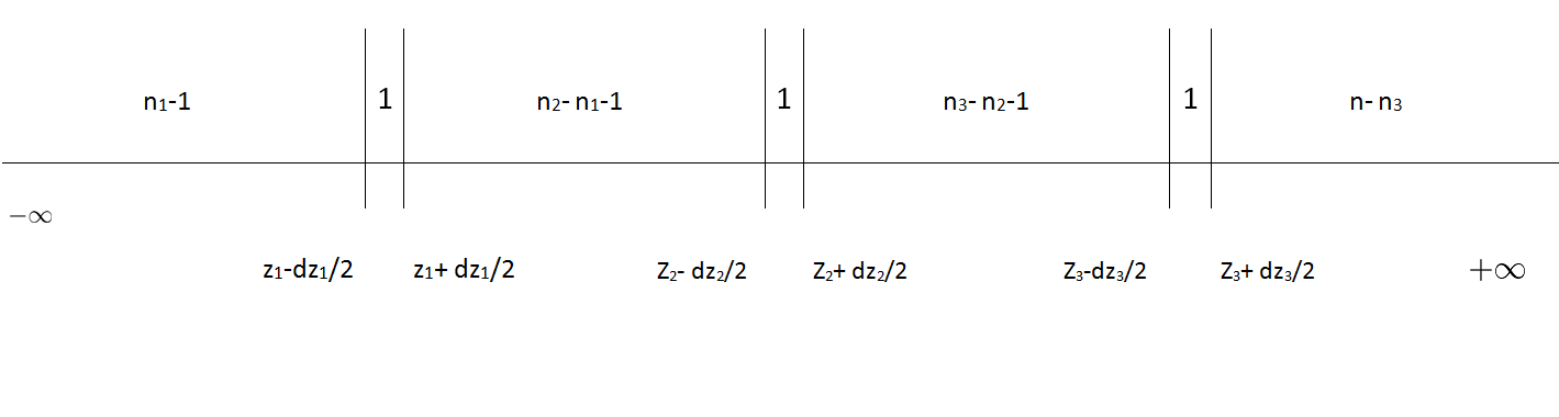
By definition, the probability density function $f_{(Z_{n_{1},n},...,Z_{n_{r},n})}$ , whenever it exists, satisfies

(4.3.2)				$\displaystyle\frac{\mathbb{P}(Z_{n_{i},n}\in]z_{1}-dz_{i}/2,z_{i}+dz_{i}/2[,\ \ 1\leq i\leq r)}{dz_{1}\times...\times dz_{r}}$
(4.3.2)			$\displaystyle=$	$\displaystyle f_{(Z_{n_{1},n},...,Z_{n_{r},n})}(z_{1},...,z_{r})(1+\varepsilon(dz_{1},...,dz_{r})),$

where $\varepsilon(dz_{1},...,dz_{r})\rightarrow 0$ as each $dz_{i}\rightarrow 0$ $(1\leq i\leq r).$ Now, by using the independence $Z_{1},...,Z_{n},$ $\mathbb{P}(Z_{n_{i},n}\in]z_{1}-dz_{i}/2,z_{i}+dz_{i}/2[,\ \ 1\leq i\leq r)$ is obtained as a multinomial probability. Using in addition the fact that $h$ is the common probability density function of $Z$ , we get

			$\displaystyle\frac{\mathbb{P}(Z_{n_{i},n}\in]z_{1}-dz_{i}/2,z_{i}+dz_{i}/2[,\ \ 1\leq i\leq r)}{dz_{1}\times...\times dz_{r}}$
		$\displaystyle=$	$\displaystyle n!\times\frac{h(z_{1})^{n_{1}-1}}{(n_{1}-1)!}\times\frac{(F(z_{2})-F(z_{1}))^{n_{2}-n_{1}-1}}{(n_{2}-n_{1}-1)!}$
		$\displaystyle\times$	$\displaystyle....\times\frac{(F(z_{j})-F(z_{j-1}))^{n_{j}-n_{j-1}-1}}{((n_{j}-n_{j-1}-1)!)}$
		$\displaystyle\times$	$\displaystyle...\times\frac{(F(z_{r})-F(z_{r-1}))^{n_{r}-n_{r-1}-1}}{(n_{r}-n_{r-1}-1)!}$
		$\displaystyle\times$	$\displaystyle\frac{(1-F(z_{r}))^{n-n_{r}}}{(n-n_{r})!}$
		$\displaystyle\times$	$\displaystyle\prod\frac{\mathbb{P}(Z_{n_{i},n}\in]z_{i}-dz_{i}/2,z_{i}+dz_{i}/2[)}{1!\ dz_{i}}$

The last factor in the latter product is

\prod_{i=1}^{r}h(z_{i})(1+dz_{i}).

By setting $n_{0}=0$ and $n_{r}=n+1$ and for $-\infty=z_{0}<z_{1}<...<z_{r}<z_{r+1}=+\infty,$

f_{(Z_{n_{1},n},...,Z_{n_{r},n})}(z_{1},...,z_{r})=n!\prod_{j=1}^{r+1}\frac{h(z_{j})(F(z_{j})-F(z_{j-1}))^{n_{j}-n_{j-1}-1}}{(n_{j}-n_{j-1}-1)!},

we see that $f_{(Z_{n_{1},n},...,Z_{n_{r},n})}$ satisfies (4.3.2). $\blacksquare$

Now, let us apply this lemma to the whole order statistics. We get this proposition.

Proposition 28.

Let $Z_{1},Z_{2},...,Z_{n}$ be $n$ independent copies of an absolutely continuous random variable $Z$ with common probability density function $h$ , and defined on the same probability space $\left(\Omega,\mathcal{A},\mathbb{P}\right)$ . The associated order statistic

(Z_{1,n},Z_{2,n},...,Z_{n,n})

has the joint probability density function

h_{\left(Z_{1,n},...,Z_{n,n}\right)}\left(z_{1,...,}z_{n}\right)=n!\prod\limits_{i=1}^{n}h\left(z_{i}\right)1_{\left(z_{1}\leq...\leq z_{n}\right).}

Proof. Let us apply Lemma 5 with $r=n$ and $n_{1}=1,n_{2}=2,...,n_{n}=n.$ Since the numbers $n_{j}-n_{j-1}-1$ vanish in (4.3.1), It comes that $Z_{1,n}<Z_{2,n}<_{.}..<Z_{n,n}$ have the joint probability density

n!\prod_{j=1}^{n}h(z_{j})1_{(z_{1}<...<z_{r}),}

$\blacksquare$

Now, we are focusing on the relation between standard uniform and exponential order statistics.

Proposition 29.

Let $n\geq 1$ be a fixed integer and $U_{1,n}\leq U_{2,n}\leq...\leq U_{n,n}$ be the order statistics associated with $U_{1},U_{2},...,U_{n},$ which are $n$ independent random variables uniformly distributed on $\left(0,1\right).$ Let $E_{1},E_{2},...,E_{n},E_{n+1},$ $\left(n+1\right)$ independent random variables following the standard exponential law, that is

\forall x\in\mathbb{R},\text{ \ }\mathbb{P}\left(E_{i}\leq n\right)=\left(1-e^{-x}\right)1_{\left(x\geq 0\right)},i=1,...,n+1.

Let $S_{j}=E_{1}+...+E_{j},$ $1\leq j\leq n+1$ . Then we have the following equality in distribution

\left(U_{1,n},U_{2,n},...,U_{n,n}\right)=^{d}\left(\frac{S_{1}}{S_{n+1}},...,\frac{S_{n}}{S_{n+1}}\right).

Proof. On one hand, by (28), the probability density function (pdf) of $U=(U_{1,n},U_{2,n},U_{n,n})$ is given by

\forall\left(u_{1},...,u_{n}\right)\in\mathbb{R}^{n},f_{U}\left(u_{1},...,u_{n}\right)=n!1_{\left(0\leq u_{1}\leq...\leq u_{n}\leq 1\right)}.

We are going to find the distribution of $Z_{n+1}^{\ast}=\left(S_{1},S_{2},...,S_{n},S_{n+1}\right)$ given $S_{n+1}=t$ , $t>0.$ We have for $y=\left(y_{1},y_{2},...,y_{n}\right)\in\mathbb{R}^{n},$

(4.3.3)		$\displaystyle f_{Z_{n}^{\ast}}^{S_{n+1}=t}\left(y\right)$	$\displaystyle=$	$\displaystyle\frac{f_{\left(Z_{n}^{\ast},S_{n+1}\right)}\left(y,t\right)}{f_{S_{n+1}}\left(t\right)}$
(4.3.3)			$\displaystyle=$	$\displaystyle\frac{f_{Z_{n+1}^{\ast}}\left(y,t\right)}{f_{S_{n+1}}\left(t\right)}\boldsymbol{1}_{\left(0\leq y_{1}\leq...\leq y_{n}\leq t\right)}.$

But $S_{n+1}$ follows a gamma law of parameters $n+1$ and $1,$ that is $S_{n+1}\sim\gamma\left(n+1,1\right),$ and its probability density function is

(4.3.4)

f_{S_{n+1}}\left(t\right)=\frac{t^{n}e^{-t}}{\Gamma\left(n+1\right)}1_{\left(t\geq 0\right)}=\frac{t^{n}}{n!}e^{-t}\boldsymbol{1}_{\left(t\geq 0\right)}.

The distribution function of $\left(S_{1},...,S_{n+1}\right)$ comes from the transformation

\left(\begin{array}[]{c}E_{1}\\ .\\ .\\ .\\ .\\ E_{n+1}\end{array}\right)=\left(\begin{array}[]{cccccc}1&&&&&\\ -1&1&&&&\\ 0&-1&1&&&\\ .&&.&.&&\\ .&&&.&.&\\ .&.&.&.&-1&1\end{array}\right)\left(\begin{array}[]{c}S_{1}\\ .\\ .\\ .\\ .\\ S_{n+1}\end{array}\right)

Let $B$ be the matrix on the formula above. The Jacobian determinant in absolute value is $\left|B\right|=1$ and

B\left(\begin{array}[]{c}y_{1}\\ .\\ .\\ y_{n+1}\end{array}\right)=\left(y_{1},y_{2}-y_{1},...,y_{n+1}-y_{n}\right).

Thus, the density of $\left(S_{1},...,S_{n+1}\right)$ is then given by

$\displaystyle f_{Z_{n+1}^{n}}(y_{1},...,y_{n+1})$	$\displaystyle=$	$\displaystyle f_{\left(E_{1},...,E_{n+1}\right)}\left(B\left(y_{1},...,y_{n+1}\right)\right)\boldsymbol{1}_{\left(0\leq y_{1}\leq...\leq y_{n}\leq y_{n+1}\right)}$
	$\displaystyle=$	$\displaystyle\prod\limits_{i=1}^{n+1}e^{-\left(y_{i}-y_{i-1}\right)}\boldsymbol{1}_{\left(0\leq y_{1}\leq...\leq y_{n}\leq y_{n+1}\right)}$
	$\displaystyle=$	$\displaystyle e^{-y_{n+1}}\boldsymbol{1}_{\left(0\leq y_{1}\leq...\leq y_{n}\leq y_{n+1}\right)}.$

where $y_{0}=0$ by convention. Going back to (4.3.3) and (4.3.4), we get , with $y=\left(y_{1},y_{2},...,y_{n}\right),$

(4.3.5)

f_{Z_{n}^{\ast}}^{S_{n+1}=t}\left(y\right)=\frac{n!}{t^{n}}\boldsymbol{1}_{\left(0\leq y_{1}\leq...\leq y_{n}\leq t\right)}.

Now, for $u=\left(u_{1},u_{2},...,u_{n}\right)\in\mathbb{R}^{n},$

f_{\left(\frac{S_{1}}{S_{n+1}},...,\frac{S_{n}}{S_{n+1}}\right)}^{S_{n+1}=t}\left(u\right)=f_{\left(\frac{S_{1}}{t},...,\frac{S_{n}}{t}\right)}^{S_{n+1}=t}\left(u_{1},u_{2},...,u_{n}\right).

This density probability function is obtained from (4.3.5) by the transform

\left(y_{1},y_{2},...,y_{n}\right)=t\left(u_{1},u_{2},...,u_{n}\right)\Longleftrightarrow\left(u_{1},u_{2},...,u_{n}\right)=\frac{1}{t}\left(y_{1},y_{2},...,y_{n}\right)

with Jacobian determinant $t^{n}.$ Then

	$\displaystyle f_{\left(\frac{S_{1}}{S_{n+1}},...,\frac{S_{n}}{S_{n+1}}\right)}^{S_{n+1}=t}\left(u_{1},u_{2},...,u_{n}\right)$	$\displaystyle=$	$\displaystyle f_{Z_{n}^{\ast}}^{S_{n+1}=t}\left(t\left(u_{1},u_{2},...,u_{n}\right)\right)t^{n}\boldsymbol{1}_{\left(0\leq tu_{1}\leq...\leq tu_{n}\leq t\right)}$
		$\displaystyle=$	$\displaystyle n!\boldsymbol{1}_{\left(0\leq u_{1}\leq...\leq u_{n}\leq 1\right)}.$

This is exactly (4.3.3). Then the conditional distribution of $Z=\left(\frac{S_{1}}{S_{n+1}},...,\frac{S_{n}}{S_{n+1}}\right)$ given $S_{n+1}=t$ does not depend on $t$ . So, its conditional distribution is also its unconditional distribution function and then

\left(\frac{S_{1}}{S_{n+1}},...,\frac{S_{n}}{S_{n+1}}\right)

has the same law as $U=(U_{1,n},U_{2,n},...,U_{n,n})$ and it is independent of $S_{n+1}$ . This puts an end to the proof.

We formalize the last conclusion in the following lemma.

Lemma 6.

Let $E_{1},E_{2},...,E_{n},E_{n+1}$ , $n\geq 1$ , be independent standard exponential random variables defined on the same probability space. Let $S_{i}=E_{1}+E+...+E_{i},1\leq i\leq n+1,$ then

\left(\frac{S_{1}}{S_{n+1}},...,\frac{S_{n}}{S_{n+1}}\right)

is independent of $S_{n+1}.$

The latter proposition exposed representations of order statistics of standard uniform random variables into that of standard exponential random variables. The following proposition reverses the situation.

Proposition 30.

Assume the notations of Proposition 29 hold. Then for any $n\geq 1,$

\left(-\log U_{1,n},...,-\log U_{n,n}\right)=_{d}\left(E_{1,n},...,E_{n,n}\right),

where $E_{1,n}\leq...\leq E_{n,n}$ are the order statistics of $E_{1},E_{2},...,E_{n},$ which are $n$ independent and exponentially distributed with intensity one.

Proof. By Proposition 28, the pdf of $E_{1,n}\leq...\leq E_{n,n}$ is

(4.3.6)

f_{Z}\left(z\right)=n!e^{-\sum_{i=1}^{n}z_{i}}\boldsymbol{1}_{\left(0\leq z_{1}\leq...\leq z_{n}\right)},\text{ }z=\left(z_{1},...,z_{n}\right)\in\mathbb{R}^{n},

where $Z=\left(E_{1,n},...,E_{n,n}\right).$ The distribution of $Z^{\ast}=\left(-\log U_{1,n},...,-\log U_{n,n}\right)$ comes from that of $U=\left(U_{1,n},...,U_{n,n}\right)$ by the diffeomorphism $\left(z_{1},...,z_{n}\right)=\left(-\log u_{1},...,-\log u_{n}\right)$ which preserves the order of the arguments and has a jacobian determinant in absolute value equal to

	$\displaystyle\left\|\frac{\partial U_{i}}{\partial z_{j}}\right\|$	$\displaystyle=$	$\displaystyle\left\|\partial\frac{\partial e^{-z_{i}}}{\partial z_{j}}\right\|=\left\|diag\left(-e^{-z_{1}},...,-e^{-z_{n}}\right)\right\|$
		$\displaystyle=$	$\displaystyle e^{-\sum_{i=1}^{n}z_{i}}.$

Then , the pdf of $Z^{\ast}$ is

	$\displaystyle f_{Z^{\ast}}\left(z_{1},...,z_{n}\right)$	$\displaystyle=$	$\displaystyle f_{U}\left(-e^{-z_{1}},...,-e^{-z_{n}}\right)e^{-\sum_{i=1}^{n}z_{i}}\boldsymbol{1}_{\left(0\leq z_{1}\leq...\leq z_{n}\right)}$
		$\displaystyle=$	$\displaystyle n!e^{-\sum_{i=1}^{n}z_{i}}\boldsymbol{1}_{\left(0\leq z_{1}\leq...\leq z_{n}\right)}.$

This pdf is that of $\left(E_{1,n},...,E_{n,n}\right)$ by (4.3.6). The proof ends here.

Another version. Let us give another version of the previous result. It is clear that for any standard uniform random variable $U,$ we have $U=^{d}1-U.$ Then for any $n\geq 1$ , we have

\left(U_{1,n},...,U_{n,n}\right)=^{d}\left(1-U_{1,n},...,1-U_{n-i+1,n},...,1-U_{n,n}\right).

The equality in distribution in Proposition 30 becomes : for any $n\geq 1$ ,

\left(-\log\left(1-U_{n,n}\right),...,-\log\left(1-U_{1,n}\right)\right)=^{d}\left(E_{1,n},...,E_{n,n}\right)

Let us go further and denote

\alpha_{i,n}=-\log\left(1-U_{i,n}\right),1\leq i\leq n.

Consider the transformation for $n\geq 1,$

\left(\begin{array}[]{l}n\alpha_{1,n}\\ \left(n-1\right)\left(\alpha_{2,n}-\alpha_{1,n}\right)\\ .\\ .\\ \left(n-i+1\right)\left(\alpha_{i,n}-\alpha_{i-1,n}\right)\\ .\\ .\\ 1\left(\alpha_{n,n}-\alpha_{n-1,n}\right)\end{array}\right)=\left(\begin{array}[]{l}V_{1}\\ V_{2}\\ .\\ .\\ V_{i}\\ .\\ \\ V_{n}\end{array}\right).

We have

\left(\begin{array}[]{l}\alpha_{1,n}\\ \alpha_{2,n}\\ .\\ .\\ .\\ .\\ \\ \alpha_{n,n}\end{array}\right)=\left(\begin{array}[]{l}V_{1}/n\\ V_{1}/n+V_{2}/\left(n-1\right)\\ .\\ .\\ .\\ .\\ \\ V_{1}/n+V_{2}/\left(n-1\right)+...+V_{n-1}/2+V_{1}/1\end{array}\right).

The probability density function of $\left(V_{1},...,V_{n}\right)$ is given by

			$\displaystyle f_{V}\left(v_{1},...,v_{n}\right)$
		$\displaystyle=$	$\displaystyle f_{(\alpha_{1,n},...,\alpha_{n,n})}\left(v_{1}/n,v_{1}/n+v2/(n-1),...,v_{1}/n+v_{2}/\left(n-1\right)+...+v_{n}\right)$
			$\displaystyle\times\left\|J\left(v\right)\right\|\times\boldsymbol{1}_{D_{V}}\left(v\right).$

The Jacobian determinant in absolute value of this transform is

\left|J\left(v\right)\right|=\frac{1}{n!}

and the domain of $V$ is

D_{V}=\mathbb{R}_{+}^{n}.

We conclude by using (4.3.6) which gives the joint pdf of $(\alpha_{1,n},...,\alpha_{n,n})$ , and by denoting $s_{i}=v_{1}/n+v2/(n-1)+...+v_{i}/(n-i+1),$ $i=1,...,n$ . We get

	$\displaystyle f_{V}\left(v_{1},...,v_{n}\right)$	$\displaystyle=$	$\displaystyle\frac{1}{n!}\times n!e^{-\sum_{i=1}^{n}s_{i}}\boldsymbol{1}_{\left(v_{1}\geq 0,..,v_{n}\geq 0\right)}$
		$\displaystyle=$	$\displaystyle e^{-\sum_{i=1}^{n}s_{i}}\boldsymbol{1}_{\left(v_{1}\geq 0,..,v_{n}\geq 0\right)}.$

We may check that $s_{1}+...+s_{n}=v_{1}+...+v_{n}.$ We arrive at

f_{V}\left(v_{1},...,v_{n}\right)=\prod\limits_{i=1}^{n}e^{-v_{i}}\boldsymbol{1}_{\left(v_{i}\geq 0\right)}.

This says that $\left(V_{1},...,V_{n}\right)$ has independent standard exponential coordinates. We summarize our finding in :

Proposition 31.

Let $\alpha_{i,n}=-\log\left(1-U_{i,n}\right),$ $i=1,...,n.$ Then the random variables

n\alpha_{1,n},\ \left(n-1\right)\left(\alpha_{2,n}-\alpha_{1,n}\right),\ldots,\left(n-i+1\right)\left(\alpha_{i,n}-\alpha_{i-1,n}\right),\dots,\left(\alpha_{n,n}-\alpha_{n-1,n}\right)

are independent standard exponential random variables.

Let us do more and put for any $1\leq i\leq n$ ,

\left(n-i+1\right)\left(\alpha_{i,n}-\alpha_{i-1,n}\right)=\left(n-i+1\right)\log\left(\frac{1-U_{i-1,n}}{1-U_{i,n}}\right).

By our previous results we have that the random variables

E_{n-i+1}^{\ast}=\left(n-i+1\right)\left(\alpha_{i,n}-\alpha_{i-1,n}\right)=\log\left(\frac{1-U_{n-i,n}}{1-U_{n-i+1,n}}\right)^{\left(n-i+1\right)}

are independent and standard exponential random variables. We may and do change $U_{n-i,n}$ to $U_{i+1,n}$ to arrive at this celebrated representation.

Proposition 32.

(Malmquist representation). Let $U_{1},U_{2},...,U_{n}$ be standard uniform random variables for $n\geq 1$ . Let $0\leq U_{1,n}<U_{2,n}<,...,<U_{n,n}\leq 1$ be their associated order statistics. Then the random variables

\log\left(\frac{U_{i+1,n}}{U_{i,n}}\right)^{i},i=1,...,n

are independent standard exponential random variables.

Chapter 5 The functional Empirical Process As a General Tools in Asymptotic Statistics

5.1. Using the small o’s and the big O’s

In this chapter, we will show how to combine all the concepts we have studied so far to get yet simple but powerful tools that may be systematically used to find asymptotic normal laws in a great variety of problems, even in current research problems. We will first study the manipulations of the $o_{\mathbb{P}}$ and the $O_{\mathbb{P}}$ symbols concerning limits in probability. Next, we present the functional empirical process that is used here only in the frame of the finite distributions case. Then, we will give some cases as illustrations.

It is important to notice for once that the methods given are valid for sequences of random variables and limit random variables defined on the same probability space. In consequence, we treat sequences of random variables $(X_{n})_{n\geq 1},$ $(Y_{n})_{n\geq 1},(Z_{n})_{n\geq 1}$ ,… defined on the same probability space $(\Omega,\mathcal{A},\mathbb{P})$ with values in $\mathbb{R}^{k}$ , $k\geq 1$ and $(a_{n})_{n\geq 1},$ $(b_{n})_{n\geq 1},(c_{n})_{n\geq 1}$ are positive random numbers.

5.2. Stochastic $o$ ’s and $O$ ’s

I - Big O’s and small o’s almost surely.

DEFINITIONS.

(a) The sequence of real random variables $(X_{n})_{n\geq 1}$ is said to be an $o$ (read the name of the letter o) of $a_{n}$ almost surely as n $\rightarrow+\infty$ , denoted by

X_{n}=o(a_{n}),a.s.\text{ as }n\rightarrow+\infty,

if and onl if

(5.2.1)

\lim_{n\rightarrow+\infty}X_{n}/a_{n}=0\text{ }a.s.

(b) The sequence of real random variables $\ (X_{n})_{n\geq 1}$ is said to be a big $O$ of $a_{n}$ almost surely as n $\rightarrow+\infty,$ denoted by

X_{n}=O(a_{n}),a.s.\text{ as }n\rightarrow+\infty,

if and only if the sequence $\{\left|X_{n}\right|/a_{n},n\geq 1\}$ is almost surely bounded, that is

(5.2.2)

\lim_{n\rightarrow+\infty}\sup\left|X_{n}\right|/a_{n}<+\infty,\text{ }a.s.

BE CAREFUL. The equality signs used in (5.2.3) and (5.2.2) are to be read in one direction only in the sense : the left member is a small $o$ of $a_{n}$ or a big $O$ of $a_{n}.$ Do not reverse the equality from left to right. For example, if $X_{n}$ is an $o(n),$ it is also an $o(n^{2})$ and we may write $o(n)=o(n^{2})$ $a.s.$ but you cannot write $o(n^{2})=o(n)$ $a.s.$ An other example : $X_{n}=n^{3/2}$ is an $o(n^{2})$ but is not an $o(n).$ This remark will extend to the notations of small $o$ ’s and big $O$ ’s in probability to be defined below.

Particular cases concerning the constants. If $a_{n}=C>0$ for any n $\geq 1,$ denoted $a_{n}\equiv C,$ we have :

(i) $X_{n}=O(C)$ a.s. if and only if $X_{n}/C$ is bounded $a.s.$ if and only if $X_{n}$ is bounded $a.s.$ and we write

X_{n}=O(1)\text{ }a.s.

(ii) $X_{n}=o(C)$ $a.s.$ if and only if $X_{n}/C$ $\rightarrow 0$ $a.s.$ if and only if $X_{n}/C\rightarrow 0$ $a.s.\$ and we write

X_{n}=o(1)\text{ }a.s.

(iii) For any constant $C>0$ , we may write $C=O(1)$ .

PROPERTIES.

The properties are very numerous and the user has often to check new ones depending on his undergoing work. But a few of them must be known and ready to be used. Let us list them in three groups.

Group A. Properties of small o’s.

(1) $o(a_{n})o(b_{n})=o(a_{n}b_{n})$ $a.s.$

(2) (1) $o(o(a_{n}))=o(a_{n})$ $a.s.$

(3) If $b_{n}\geq a_{n}$ for all $n\geq 1,o(a_{n})=o(b_{n})$ $a.s.$

(4) $o(a_{n})+o(a_{n})=o(a_{n})$ $a.s.$

(5) $o(a_{n})+o(b_{n})=o(a_{n}+b_{n})$ $a.s.$ and $o(a_{n})+o(b_{n})=o(a_{n}\vee b_{n})$ $a.s.$ where $a_{n}\vee b_{n}=\max(a_{n},b_{n}).$

(6) $o(a_{n})=a_{n}o(1)$ $a.s.$ and $a_{n}o(1)=o(a_{n})$ $a.s.$

PROOFS. Each of these properties is quickly proved in :

(1) If

$X_{n}=o(a_{n})$ and $Y_{n}=o(b_{n}),$ then

\lim_{n\rightarrow+\infty}\frac{\left|X_{n}Y_{n}\right|}{a_{n}b_{n}}=\lim_{n\rightarrow+\infty}\frac{\left|X_{n}\right|}{a_{n}}\times\lim_{n\rightarrow+\infty}\frac{\left|Y_{n}\right|}{b_{n}}=0\text{ }a.s

and then $X_{n}Y_{n}=o(a_{n}b_{n})$ $a.s.$

(2) If $Y_{n}=o(a_{n}),$ $a.s.$ and $X_{n}=o(Y_{n}),$ $a.s.,$

\lim_{n\rightarrow+\infty}\frac{\left|X_{n}\right|}{a_{n}}=\lim_{n\rightarrow+\infty}\left|\frac{X_{n}}{Y_{n}}\right|\times\frac{\left|Y_{n}\right|}{a_{n}}=\lim_{n\rightarrow+\infty}\left|\frac{X_{n}}{Y_{n}}\right|\times\lim_{n\rightarrow+\infty}\frac{\left|Y_{n}\right|}{a_{n}}=0,

that is $X_{n}=o(a_{n})$ $a.s.$

(3) If

$X_{n}=o(a_{n})$ and $b_{n}\geq a_{n}$ for all n $\geq 1,$ then

0\leq\lim_{n\rightarrow+\infty}\sup\frac{\left|X_{n}\right|}{b_{n}}=\lim_{n\rightarrow+\infty}\sup\frac{\left|X_{n}\right|}{a_{n}}\frac{a_{n}}{b_{n}}\leq\lim_{n\rightarrow+\infty}\sup\frac{\left|X_{n}\right|}{a_{n}}=0\text{ }a.s

and $\left|X_{n}/b_{n}\right|\rightarrow 0$ $a.s.,$ that is $X_{n}=o(b_{n}),$ $a.s.$

(4) If

$X_{n}=o(a_{n})$ and $Y_{n}=o(a_{n}),$ then

\lim_{n\rightarrow+\infty}\sup\frac{\left|X_{n}+Y_{n}\right|}{a_{n}}\leq\lim_{n\rightarrow+\infty}\frac{\left|X_{n}\right|}{a_{n}}+\lim_{n\rightarrow+\infty}\frac{\left|Y_{n}\right|}{b_{n}}=0\text{ }a.s

and then $X_{n}+Y_{n}=o(a_{n})$ $a.s.$

(5) To prove that $o(a_{n})+o(b_{n})=o(a_{n}+b_{n})$ $a.s.$ , use Point (3) to see that $o(a_{n})=o(a_{n}+b_{n})$ $a.s.$ since $a_{n}+b_{n}\geq a_{n}$ for all $n\geq 1$ and as well $\ o(b_{n})=o(a_{n}+b_{n})$ $a.s.$ and then use Point (3) to conclude. We prove that $o(a_{n})+o(b_{n})=o(a_{n}\vee b_{n})$ $a.s.$ in the very same manner.

(6) This is a simple rephrasing of the definition.

Group B. Properties of big $O$ ’s.

(1) $O(a_{n})O(b_{n})=O(a_{n}b_{n})$ $a.s.$

(2) $O(O(a_{n}))=O(a_{n})$ $a.s.$

(3) If $b_{n}\geq a_{n}$ for all $n\geq 1,O(a_{n})=O(b_{n})$ $a.s.$

(4) $O(a_{n})+O(a_{n})=O(a_{n})$ $a.s.$

(5) $O(a_{n})+O(b_{n})=O(a_{n}+b_{n})$ $a.s.$ and $O(a_{n})+O(b_{n})=O(a_{n}\vee b_{n})$ $a.s.$ , where $a_{n}\vee b_{n}=\max(a_{n},b_{n}).$

(6) $O(a_{n})=a_{n}O(1)$ $a.s.,$ and $a_{n}O(1)=O(a_{n})$ $a.s.$

PROOFS. These properties are proved exactly as those of Group A, where superior limits are used at the place of limits.

Group C. Properties of combinations of small o’s and big O’s.

(1) $o(a_{n})O(b_{n})=o(a_{n}b_{n})$ $a.s.$

(2) $o(O(a_{n}))=o(a_{n})$ $a.s.$ and $O(o(a_{n}))=o(a_{n}),$ $a.s.$

(3a) If $a_{n}=O(b_{n}),$ $a.s.,$ then $o(a_{n})+O(b_{n})=O(b_{n})$ $a.s.$

(3b) If $b_{n}=O(a_{n}),$ $a.s.,$ then $o(a_{n})+O(b_{n})=O(a_{n})$ $a.s.$

(3c) If $b_{n}=o(a_{n}),$ $a.s.,$ then $o(a_{n})+O(b_{n})=o(b_{n})$ $a.s.$

(4) $(1+o(a_{n}))^{-1}-1=O(a_{n})$ , $a.s.$

PROOFS.

(1) If $X_{n}=o(a_{n})$ and $Y_{n}=O(b_{n}),$ then

\lim_{n\rightarrow+\infty}\sup\frac{\left|Y_{n}\right|}{b_{n}}=C<+\infty\text{ }a.s.

and

	$\displaystyle\lim_{n\rightarrow+\infty}\sup\frac{\left\|X_{n}Y_{n}\right\|}{a_{n}b_{n}}$	$\displaystyle=$	$\displaystyle\lim_{n\rightarrow+\infty}\left(\left\|\frac{X_{n}}{a_{n}}\right\|\times\frac{\left\|Y_{n}\right\|}{b_{n}}\right)=\lim_{n\rightarrow+\infty}\sup\left\|\frac{X_{n}}{a_{n}}\right\|\times\lim_{n\rightarrow+\infty}\sup\frac{\left\|Y_{n}\right\|}{b_{n}}$
		$\displaystyle\leq$	$\displaystyle C\lim_{n\rightarrow+\infty}\sup\left\|\frac{X_{n}}{a_{n}}\right\|=0\text{ }a.s.$

(2) Use Points (6) of Groups A and B to say

o(O(a_{n}))=o(1)\times O(a_{n})=a_{n}\times o(1)\times O(1)=a_{n}\times o(1)=o(a_{n})

and

O(o(a_{n}))=o(a_{n})O(1)=a_{n}\times o(1)\times O(1)=a_{n}\times o(1)=o(a_{n}).

(3a-b-c) These three points are proved in similar ways. Let us give the details of (3b) for example. Let $X_{n}=o(a_{n})$ and $Y_{n}=O(b_{n})$ and $b_{n}=O(a_{n}).$ Then

	$\displaystyle o(a_{n})+O(b_{n})$	$\displaystyle=$	$\displaystyle o(a_{n})+O(O(a_{n}))=o(a_{n})+O(a_{n})$
		$\displaystyle=$	$\displaystyle a_{n}(o(1)+O(1))=a_{n}\times O(1)=O(a_{n}).$

(4) We have

	$\displaystyle(1+o(a_{n}))^{-1}-1$	$\displaystyle=$	$\displaystyle\frac{o(a_{n})}{1+o(a_{n})}=o(a_{n})O(1)$
		$\displaystyle=$	$\displaystyle a_{n}o(1)O(1)=a_{n}o(1)=o(a_{n}).$

II - Big $O$ ’s and small $o$ ’s in probability.

DEFINITIONS.

(a) The sequence of real random variables $(X_{n})_{n\geq 1}$ is said to be an o (read the name of the letter o) of $a_{n}$ in probability as n $\rightarrow+\infty,$ denoted by

X_{n}=o_{\mathbb{P}}(a_{n}),\text{ as }n\rightarrow+\infty,

if and only if

(5.2.3)

\lim_{n\rightarrow+\infty}X_{n}/a_{n}=0\text{ in probability},

that is for any $\lambda>0$

\lim_{n\rightarrow+\infty}\mathbb{P}(\left|X_{n}\right|>\lambda a_{n})=0.

(b) The sequence of real random variables $\ (X_{n})_{n\geq 1}$ is said to be a big O of $a_{n}$ in probability as n $\rightarrow+\infty,$ denoted by

X_{n}=O_{\mathbb{P}}(a_{n}),\text{ as }n\rightarrow+\infty,

if and only if the sequence $\{\left|X_{n}\right|/a_{n},n\geq 1\}$ is bounded in probability, that is : For any $\varepsilon>0,$ there exists a constant $\lambda>0$ , such that

(5.2.4)

\inf_{n\geq 1}\mathbb{P}(\left|X_{n}\right|\leq\lambda a_{n})\geq 1-\varepsilon,

which is equivalent to

(5.2.5)

\liminf_{\lambda\uparrow+\infty}\limsup_{n\rightarrow+\infty}\mathbb{P}(\left|X_{n}\right|>\lambda a_{n})=0.

Before we go further, let us prove the following Lemma.

Lemma 7.

Each of (5.2.4) and (5.2.5) is equivalent to : For any $\varepsilon>0,$ there exists an integer $N\geq 1$ a constant $\lambda>0$ , such that

(5.2.6)

\inf_{n\geq N}\mathbb{P}(\left|X_{n}\right|\leq\lambda a_{n})\geq 1-\varepsilon.

PROOF. To prove that (5.2.4) and (5.2.6) are equivalent, it will be enough to show that (5.2.6) $\Longrightarrow$ (5.2.4) since the reverse implication is obvious. Suppose that (5.2.6), that is, for $\varepsilon>0,$ there exist $N\geq 1$ and a real number $\lambda_{0}>0$ such that

(5.2.7)

\forall(n\geq N),\text{ }\mathbb{P}(\left|X_{n}/a_{n}\right|\leq\lambda_{0})\geq 1-\varepsilon.

If $N=1,$ then (5.2.4) holds. If not, we have for $j\in\{1,...,N-1\}$ fixed, $(\left|X_{j}/a_{j}\right|\leq\lambda)\uparrow\Omega$ as $\lambda\uparrow+\infty.$ So by the Monotone Convergence Theorem, there exists for each $j\in\{1,...,N-1\}$ a real number $\lambda_{j}>0$ such that $\mathbb{P}(\left|X_{j}/a_{j}\right|\leq\lambda_{j})>1-\varepsilon$ . We take $\lambda=\max(\lambda_{0},\lambda_{1},...,\lambda_{N-1})$ and get

\forall(n\geq 1),\text{ }\mathbb{P}(\left|X_{n}/a_{n}\right|\leq\lambda)\geq 1-\varepsilon,

which is (5.2.4). Now, let us prove that (5.2.5) $\Longleftrightarrow$ (5.2.6). First (5.2.5) means

\lim_{\lambda\uparrow+\infty}\limsup_{n\rightarrow+\infty}\mathbb{P}(\left|X_{n}\right|>\lambda a_{n})=0,

since $\limsup_{n\rightarrow+\infty}\mathbb{P}(\left|X_{n}\right|>\lambda a_{n})$ in non-increasing as $\lambda\uparrow+\infty$ on $[0,1]$ .

We get for any $\varepsilon>0,$ there exists a real number $\lambda>0$ such that

\limsup_{n\rightarrow+\infty}\mathbb{P}(\left|X_{n}\right|>\lambda a_{n})=\lim_{N\uparrow+\infty}\sup_{n\geq N}\mathbb{P}(\left|X_{n}\right|>\lambda a_{n})\leq\varepsilon/2.

Then for some $N>0$ ,

\sup_{n\geq N}\mathbb{P}(\left|X_{n}\right|>\lambda a_{n})\leq\varepsilon,

that is

\inf_{n\geq N}\mathbb{P}(\left|X_{n}\right|\leq\lambda a_{n})\geq 1-\varepsilon,

which is (5.2.6). Now, a rephrasing of this gives : for any $\varepsilon>0,$ there exists $N_{0}>0$ and a real number $\lambda_{0}>0$ such that

(5.2.8)

\inf_{n\geq N}\mathbb{P}(\left|X_{n}\right|\leq\lambda_{0}a_{n})\geq 1-\varepsilon,

that is

\sup_{n\geq N}\mathbb{P}(\left|X_{n}\right|>\lambda_{0}a_{n})<\varepsilon,

which leads to

\inf_{N\geq 1}\sup_{n\geq N}\mathbb{P}(\left|X_{n}\right|>\lambda_{0}a_{n})<\varepsilon,

and next

\inf_{\lambda>0}\inf_{N\geq 1}\sup_{n\geq N}\mathbb{P}(\left|X_{n}\right|>\lambda a_{n})<\varepsilon,

which is (5.2.5).

COMMENTS, NOTATIONS AND SOMME LEMMAS.

(a) From Chapter 3, an $O_{\mathbb{P}}(1)$ is simply a tight sequence of random variables. From Theorem 7 of Chapter 3, we have that any sequence $X_{n}=O_{\mathbb{P}}(a_{n})$ contains a sub-sequence $(X_{n_{k}})_{k\geq 1}$ such that $(X_{n_{k}}/a_{n_{k}})_{k\geq 1}$ weakly converges in $\mathbb{R}$ .

(b) It may be convenient to rephrase (5.2.4) into the following sentence.

For any $\varepsilon>0$ there exists a real number $\lambda>0$ such that $\left|X_{n}\right|\leq\lambda a_{n}$ With Probability At Least Equal to $1-\varepsilon$ for all $n\geq 1$ .

By using the complementary events, we will say : for any $\varepsilon>0$ there exists a real number $\lambda>0$ such that $\left|X_{n}\right|>\lambda a_{n}$ With Probability At Most Equal to $\varepsilon$ for all $n\geq 1$ .

With Probability At Least Equal to $1-\varepsilon$ will be abbreviated by $WPALE(1-\varepsilon)$ .

As well, $WPAME(\varepsilon)$ is an abbreviation of With Probability At Most Equal to $\varepsilon$ .

For lengthy demonstrations, using these types of sentences described above may be handy.

We will need two other lemmas.

Lemma 8.

We have the following properties :

(a) If $X_{n}$ is a sequence of $k-$ random vectors weakly converging (say, to a $k$ -random vector $X$ ), then $\left\|X_{n}\right\|=O_{\mathbb{P}}(1)$ .

(b) Let $X_{n}$ be a sequence of random vectors with values in the metric space $(S,d)$ converging in probability to a constant $C\in S$ and let $g$ be a measurable mapping from $(S,d)$ to another metric space $(E,r)$ . If $g$ is continuous at $C$ , then $g(X_{n})$ converges in probability to $C$ .

(c) Consider a sequence of $k-$ random vectors $(X_{n})_{n\geq 1}$ converging to zero in probability. Let $R(x)$ be a real function of $x\in\mathbb{R}^{k}$ continuous at zero and such that $R(0)=0$ . Let $p>0$ be a fixed integer. If $R(x)=o(\|x\|^{p})$ as $x\rightarrow 0$ , then $R(X_{n})=o_{\mathbb{P}}(\|X_{n}\|^{p}).$ If $R(x)=O(\|x\|^{p})$ as $x\rightarrow 0\$ , then $R(X_{n})=O_{\mathbb{P}}(\|X_{n}\|^{p})$ .

Proof.

Proof of Point (a). If $X_{n}\rightarrow_{\mathbb{P}}X$ , then by Proposition 12, $X_{n}\rightarrow_{w}X$ and by the continuous mapping Theorem 7 of Chapter 2, $\left\|X_{n}\right\|\rightarrow_{w}\left\|X\right\|.$ Then by Theorem 3, we have for any continuity point of $F_{\left\|X\right\|}(\lambda)=P(\left\|X\right\|\leq\lambda),$

\lim_{n\rightarrow+\infty}\mathbb{P}\left(\left|X_{n}\right|>\lambda\right)=\mathbb{P}\left(\left\|X\right\|>\lambda\right)=F_{\left\|X\right\|}(\lambda).

Since the set of discontinuity points of $F_{\left\|X\right\|}$ is at most countable (see Point 6 of Chapter 4, Section 4.1), apply the formula above for $\lambda\rightarrow+\infty$ while $\lambda$ are continuity points. Since $1-F_{\left\|X\right\|}(\lambda)\rightarrow 0$ as $\lambda\rightarrow+\infty,$ then for any $\varepsilon>0,$ we are able to pick one value of $\lambda(\varepsilon)$ which is a continuity point of $F_{\left\|X\right\|}$ satisfying $1-F_{\left\|X\right\|}(\lambda)<\varepsilon.$ For any $\varepsilon>0,$ we have found $\lambda(\varepsilon)>0$ such that

\limsup_{n\rightarrow+\infty}\mathbb{P}\left(\left|X_{n}\right|>\lambda(\varepsilon)\right)\leq\varepsilon,

which implies

\lim_{\lambda\rightarrow+\infty}\limsup_{n\rightarrow+\infty}\mathbb{P}\left(\left|X_{n}\right|>\lambda\right)=0.

Point (a) is proved.

Proof of Point (b). Assume the notations of this point and suppose that $g$ is continous at $C$ . Let $\varepsilon>0.$ By the continuity of $g$ at $C$ , there exists $\eta>0$ such that

d(x,C)<\eta\Longrightarrow r(g(x),g(C))<\varepsilon/2.

Now

$\displaystyle\mathbb{P}(r(g(X_{n}),g(C)$	$\displaystyle>$	$\displaystyle\varepsilon)=\mathbb{P}(\left\{r(g(X_{n}),g(C)>\varepsilon\right\}\cap\left\{d(X_{n},C)\geq\eta\right\})$
	$\displaystyle+$	$\displaystyle\mathbb{P}(\left\{r(g(X_{n}),g(C)>\varepsilon\right\}\cap\left\{d(X_{n},C)<\eta\right\})$
	$\displaystyle\leq$	$\displaystyle\mathbb{P}(d(X_{n},C)\geq\eta),$

since $(\left\{r(g(X_{n}),g(C)>\lambda\right\}\cap\left\{d(X_{n},C)<\eta\right\})\subset$ $(\left\{r(g(X_{n}),g(C)>\varepsilon\right\}\cap\left\{d(X_{n},C)<\eta\right\}\cap\left\{\left\{r(g(X_{n}),g(C)<\varepsilon/2\right\}\right\})=\emptyset$ .

Then, since $X_{n}\rightarrow_{\mathbb{P}}C$ , we have

\limsup_{n\rightarrow+\infty}\mathbb{P}(r(g(X_{n}),g(C)>\varepsilon)\leq\limsup_{n\rightarrow+\infty}\mathbb{P}(d(X_{n},C)\geq\eta)=0.

So Point (b) is true.

Proof of Point (c-1). Let $R(x)=o(\|x\|^{p})$ as $x\rightarrow 0$ . Then

g(x)=\left|R(x)/\|x\|^{p}\right|\rightarrow 0

as $x\rightarrow 0$ . This proves that $g(0)=0$ , and that $g$ is continuous at zero. By continuity of $g$ at zero and by Point (a), we have, as $n\rightarrow+\infty$ , that $g(X_{n})=\left|R(X_{n})\right|/\|X_{n}\|^{p}\rightarrow_{\mathbb{P}}0$ whenever $X_{n}\rightarrow_{\mathbb{P}}0$ .

Hence $R(X_{n})=o_{\mathbb{P}}(\|X_{n}\|^{p})$ .

Proof of Point (c-2). Let $R(x)=O(\|x\|^{p})$ as $x\rightarrow 0.$ Then for any $\varepsilon>0,$ there exist $\eta>0$ and $C>0$ such $\left|R(x)\right|/\|x\|^{p}\leq C$ for all $\left\|x\right\|<\eta.$ Then for $\lambda>C,$

$\displaystyle\mathbb{P}(\left\|R(X_{n})\right\|/\\|X_{n}\\|^{p}$	$\displaystyle>$	$\displaystyle\lambda)=\mathbb{P}(\left\{\left\|R(X_{n})\right\|/\\|X_{n}\\|^{p}>\lambda\right\}\cap\left\{\left\\|X_{n}\right\\|\geq\eta\right\})$
	$\displaystyle+$	$\displaystyle\mathbb{P}(\left\{\left\|R(X_{n})\right\|/\\|X_{n}\\|^{p}>\lambda\right\}\cap\left\{\left\\|X_{n}\right\\|<\eta\right\})$
	$\displaystyle\leq$	$\displaystyle\mathbb{P}(\left\\|X_{n}\right\\|\geq\eta),$

since $(\left\{\left|R(X_{n})\right|/\|X_{n}\|^{p}>\lambda\right\}\cap\left\{\left\|X_{n}\right\|<\eta\right\})\subset(\left\{\left|R(X_{n})\right|/\|X_{n}\|^{p}>\lambda\right\}\cap\left\{\left\|X_{n}\right\|<\eta\right\}\cap\left\{\left\{\left|R(X_{n})\right|/\|X_{n}\|^{p}<C\right\}\right\})=\emptyset.$ Then for all $\lambda>C,$

\limsup_{n\rightarrow+\infty}\mathbb{P}(\left|R(X_{n})\right|/\|X_{n}\|^{p}>\lambda)=0

and then

\lim_{\lambda\rightarrow+\infty}\limsup_{n\rightarrow+\infty}\mathbb{P}(\left|R(X_{n})\right|/\|X_{n}\|^{p}>\lambda)=0.

We conclude that $\left|R(X_{n})\right|/\|X_{n}\|^{p}=O_{\mathbb{P}}(1)$ .

In some situations, we would be able to work with convergence in probability while we are not sure of measurability of some sequences. For example, using the Mean Value Theorem with real random sequences $X_{n}$ and $Z_{n}$ and real function $g$ of class $C^{1}$ may lead to this kind of formula

g(X_{n})-g(Y_{n})=(X_{n}-Y_{n})g^{\prime}(Z_{n}),

with $\min(X_{n},Y_{n})\leq Z_{n}\leq\max(X_{n},Y_{n}).$ Here, we know that $g^{\prime}(Z_{n})$ is measurable but we do not know if $Z_{n}$ is. In such a situation, we may need the notion of outer probability.

Definition 4.

Let $(u_{n})_{n\geq 1}$ be a sequence of real-valued applications defined on $\Omega.$ It has a measurable covering sequence if and only if there exists a sequence of non-negative real random variables $(v_{n})_{n\geq 1}$ defined on $(\Omega,\mathcal{A})$ such that

\forall(n\geq 1),u_{n}\leq v_{n}.

Next, $(u_{n})_{n\geq 1}$ converges in outer probability to a real-valued application $u$ defined on $\Omega$ , as $n\rightarrow+\infty,$ if and only the sequence $(u_{n}-u)_{n\geq 1}$ has a measurable covering sequence $(v_{n})_{n\geq 1}$ which converges to zero in probability, and we denote

u_{n}\rightarrow_{\mathbb{P}^{\ast}}u\text{ as }n\rightarrow+\infty.

We are going to see that the result of Point (b) of the lemma above still holds for convergence in outer probability in the special case of $\mathbb{R}$ .

Lemma 9.

Let $X_{n}$ be a sequence of real-valued applications defined on $\Omega$ converging in outer probability to $c\in\mathbb{R}$ . Let $g$ be a real-valued function defined on $\mathbb{R},$ continuous at $c$ and such that for each $n\geq 1,$ $g(X_{n})$ is measurable. Then $g(X_{n})$ converges in probability to $g(c)$ .

Proof. Assume the notations of the lemma. Let $Y_{n}$ be a sequence of random variables such that $\left|X_{n}-c\right|\leq Y_{n}$ for all $n\geq 1$ and $Y_{n}\rightarrow 0$ in probability.

Now, by the continuity of $g$ at $c$ , there exists $\eta>0$ such that

\left|x-c\right|<\eta\Longrightarrow\left|g(x)-g(c)\right|<\varepsilon/2.

$\displaystyle\mathbb{P}(\left\|g(X_{n})-g(c)\right\|>\varepsilon)$	$\displaystyle=$	$\displaystyle\mathbb{P}(\left\{r(g(X_{n}),g(C)>\varepsilon\right\}\cap\left\{Y_{n}\geq\eta\right\})$
	$\displaystyle+$	$\displaystyle\mathbb{P}(\left\{\left\|g(X_{n})-g(c)\right\|>\varepsilon\right\}\cap\left\{Y_{n}<\eta\right\})$
	$\displaystyle\leq$	$\displaystyle\mathbb{P}(\left\{Y_{n}\geq\eta\right\})$

since $\left\{\left|g(X_{n})-g(c)\right|>\varepsilon\right\}\cap\left\{Y_{n}<\eta\right\}=\emptyset.$ The reason on this is that on $\left\{\left|g(X_{n})-g(c)\right|>\varepsilon\right\}\cap\left\{Y_{n}<\eta\right\},$ we have $\left|X_{n}-c\right|\leq Y_{n}<\eta$ and then $\left|g(X_{n})-g(c)\right|<\varepsilon/2.$ This is impossible. Next, since $Y_{n}\rightarrow_{\mathbb{P}}0,$ we have

\lim\sup_{n\rightarrow+\infty}\mathbb{P}(\left|g(X_{n})-g(c)\right|>\varepsilon)\leq\lim\sup_{n\rightarrow+\infty}\mathbb{P}(Y_{n}\geq\eta)=0.

The proof is complete.

Now, we may give some important properties of the small $o^{\prime}s$ and the big $O^{\prime}s$ in probability.

MAIN PROPERTIES.

(1) If $X_{n}=o(1)$ $a.s.,$ then $X_{n}=o_{\mathbb{P}}(1)$ .

(2) $o_{\mathbb{P}}(a_{n})=a_{n}o_{\mathbb{P}}(1)$ and $a_{n}o_{\mathbb{P}}(1)=o_{\mathbb{P}}(a_{n})$ .

(3) $o_{\mathbb{P}}(a_{n})o_{\mathbb{P}}(b_{n})=o_{\mathbb{P}}(a_{n}b_{n})$ .

(4) $o_{\mathbb{P}}(o_{\mathbb{P}}(a_{n}))=o_{\mathbb{P}}(a_{n})$ .

(5) If $b_{n}\geq a_{n}$ for all $n\geq 1,o_{\mathbb{P}}(a_{n})=o_{\mathbb{P}}(b_{n})$ .

(6) $o_{\mathbb{P}}(a_{n})+o_{\mathbb{P}}(a_{n})=o_{\mathbb{P}}(a_{n})$ .

(7) $o_{\mathbb{P}}(a_{n})+o_{\mathbb{P}}(b_{n})=o_{\mathbb{P}}(a_{n}+b_{n})$ and $o_{\mathbb{P}}(a_{n})+o_{\mathbb{P}}(b_{n})=o_{\mathbb{P}}(a_{n}\vee b_{n})$ , where $a_{n}\vee b_{n}=\max(a_{n},b_{n})$ .

(8) If $X_{n}=O(1)$ $a.s.,$ then $X_{n}=O_{\mathbb{P}}(1)$ .

(9) $O_{\mathbb{P}}(a_{n})=a_{n}O_{\mathbb{P}}(1)$ .

(10) $O_{\mathbb{P}}(a_{n})O_{\mathbb{P}}(b_{n})=O_{\mathbb{P}}(a_{n}b_{n})$ .

(11) $O_{\mathbb{P}}(O_{\mathbb{P}}(a_{n}))=O_{\mathbb{P}}(a_{n})$ .

(12) If $b_{n}\geq a_{n}$ for all $n\geq 1,O_{\mathbb{P}}(a_{n})=O_{\mathbb{P}}(b_{n})$ .

(13) $O_{\mathbb{P}}(a_{n})+O_{\mathbb{P}}(a_{n})=O_{\mathbb{P}}(a_{n})$ .

(14) $O_{\mathbb{P}}(a_{n})+O_{\mathbb{P}}(b_{n})=O_{\mathbb{P}}(a_{n}+b_{n})$ and $O_{\mathbb{P}}(a_{n})+O_{\mathbb{P}}(b_{n})=O_{\mathbb{P}}(a_{n}\vee b_{n})$ where $a_{n}\vee b_{n}=\max(a_{n},b_{n})$ .

(15) $o_{\mathbb{P}}(a_{n})O_{\mathbb{P}}(b_{n})=o_{\mathbb{P}}(a_{n}b_{n})$ .

(16) $o_{\mathbb{P}}(O_{\mathbb{P}}(a_{n}))=o_{\mathbb{P}}(a_{n})$ and $O_{\mathbb{P}}(o_{\mathbb{P}}(a_{n}))=o_{\mathbb{P}}(a_{n})$ .

(17a) If $a_{n}=O_{\mathbb{P}}(b_{n})$ , then $o(a_{n})+O_{\mathbb{P}}(b_{n})=O_{\mathbb{P}}(b_{n})$ .

(17b) If $b_{n}=O_{\mathbb{P}}(a_{n})$ , then $o_{\mathbb{P}}(a_{n})+O_{\mathbb{P}}(b_{n})=O_{\mathbb{P}}(a_{n})$ .

(17c) If $b_{n}=o_{\mathbb{P}}(a_{n}),$ $a.s.$ , then $o(a_{n})+O_{\mathbb{P}}(b_{n})=o(b_{n})$ .

(18) $(1+o_{\mathbb{P}}(a_{n}))^{-1}-1=o_{\mathbb{P}}(a_{n})$ .

(19) An $o_{\mathbb{P}}(1)$ is an $O_{\mathbb{P}}(1)$ .

PROOFS.

(1) This derived from the implication : $X_{n}\rightarrow 0$ a.s. $\Longrightarrow X_{n}\rightarrow_{P}0$ (See Proposition 12).

(2) We have :

$X_{n}=o_{\mathbb{P}}(a_{n})\Longleftrightarrow\left|X_{n}/a_{n}\right|\longrightarrow_{P}0\Longleftrightarrow X_{n}/a_{n}=o_{\mathbb{P}}(1)\Longleftrightarrow X_{n}=a_{n}o_{\mathbb{P}}(1).$

(3) By Point (2) above, $o_{\mathbb{P}}(a_{n})o_{\mathbb{P}}(b_{n})=a_{n}b_{n}\times o_{\mathbb{P}}(1)o_{\mathbb{P}}(1)=a_{n}b_{n}\times o_{\mathbb{P}}(1)=o_{\mathbb{P}}(a_{n}b_{n})$ (Check $o_{\mathbb{P}}(1)o_{\mathbb{P}}(1)=o_{\mathbb{P}}(1)$ in Property (A1) in the Appendix subsection below).

(4) $o_{\mathbb{P}}(o_{\mathbb{P}}(a_{n}))=o_{\mathbb{P}}(a_{n})o_{\mathbb{P}}(1)=a_{n}\times o_{\mathbb{P}}(1)o_{\mathbb{P}}(1)=a_{n}\times o_{\mathbb{P}}(1)=o_{\mathbb{P}}(a_{n})$ (Again, use Property (A1) of the Appendix subsection below).

(5) Let $b_{n}\geq a_{n}$ for all $n\geq 1,X_{n}=o_{\mathbb{P}}(a_{n}).$ For any $\eta>0,0\leq\lim_{n\rightarrow+\infty}\sup P(\left|X_{n}/b_{n}\right|>\eta)\leq\lim_{n\rightarrow+\infty}P(\left|X_{n}/a_{n}\right|>\eta)=0.$

(6) Let $X_{n}=o_{\mathbb{P}}(a_{n})$ and $Y_{n}=o_{\mathbb{P}}(a_{n}).$ Use the classical stuff, for $\eta>0,$

\left(\frac{\left|X_{n}\right|}{a_{n}}>\eta/2\right)\cap\left(\frac{\left|Y_{n}\right|}{a_{n}}>\eta/2\right)\subset\left(\frac{\left|X_{n}+Y_{n}\right|}{a_{n}}>\eta\right).

Then for $\eta>0,$

(5.2.9)		$\displaystyle\limsup_{n\rightarrow+\infty}\mathbb{P}\left(\frac{\left\|X_{n}+Y_{n}\right\|}{a_{n}}>\eta\right)$	$\displaystyle\leq$	$\displaystyle\limsup_{n\rightarrow+\infty}\mathbb{P}\left(\frac{\left\|X_{n}\right\|}{a_{n}}>\eta/2\right)$
(5.2.9)			$\displaystyle+$	$\displaystyle\limsup_{n\rightarrow+\infty}\mathbb{P}\left(\frac{\left\|Y_{n}\right\|}{a_{n}}>\eta/2\right)=0.$

(7) To prove this point, combine Points (5) and (6) above.

(8) $X_{n}=O(1)$ $a.s.$ as $n\rightarrow+\infty$ means there exists $\Omega_{0}$ measurable such that $\mathbb{P}(\Omega_{0})=1$ and for any $\omega\in\Omega_{0},$

\limsup_{n\rightarrow+\infty}\left|X_{n}(\omega)\right|=\inf_{n\geq 1}\sup_{p\geq n}\left|X_{p}\right|=M(\omega)<+\infty.

We have for all $n\geq 1,$

\mathbb{P}\left(\left|X_{n}\right|>\lambda\right)\leq\mathbb{P}\left(\sup_{p\geq n}\left|X_{p}\right|>\lambda\right).

We have $Y_{n}=\sup_{p\geq n}\left|X_{p}\right|\downarrow M$ $a.s.$ Then $Y_{n}1_{\Omega_{0}}\rightarrow_{\mathbb{P}}M1_{\Omega_{0}}$ . We are dealing with real random variables and we may apply the weak convergence results. We get $Y_{n}1_{\Omega_{0}}\rightarrow_{w}M1_{\Omega_{0}}$ by Proposition 12. By Theorem 3, we have for any continuity point of $F_{M}(\lambda)=P(M1_{\Omega_{0}}\leq\lambda)$ . Use the Monotone Convergence Theorem to get

$\displaystyle\limsup_{n\rightarrow+\infty}\mathbb{P}\left(\left\|X_{n}\right\|>\lambda\right)$	$\displaystyle=$	$\displaystyle\limsup_{n\rightarrow+\infty}\mathbb{P}\left(\sup_{p\geq n}\left\|X_{p}\right\|1_{\Omega_{0}}>\lambda\right)$
	$\displaystyle=$	$\displaystyle\limsup_{n\rightarrow+\infty}\mathbb{P}\left(\sup_{p\geq n}\left\|X_{p}\right\|1_{\Omega_{0}}>\lambda\right)$
	$\displaystyle=$	$\displaystyle\mathbb{P}\left(M1_{\Omega_{0}}>\lambda\right)$
	$\displaystyle=$	$\displaystyle 1-F_{M}(\lambda).$

Since the set of discontinuity points of $F_{M}$ is at most countable (see Point 6 of Chapter 4), we apply the formula above for $\lambda\rightarrow+\infty$ while $\lambda$ are continuity points. Since $1-F_{M}(\lambda)\rightarrow 0$ as $\lambda\rightarrow+\infty,$ then for any $\varepsilon>0,$ we are able to pick one value of $\lambda(\varepsilon)$ which is a continuity point of $F_{M}$ satisfying $1-F_{M}(\lambda)<\varepsilon$ . For any $\varepsilon>0$ , we have found $\lambda(\varepsilon)>0$ such that

\limsup_{n\rightarrow+\infty}\mathbb{P}\left(\left|X_{n}\right|>\lambda(\varepsilon)\right)\leq\varepsilon,

which implies

\lim_{\lambda\rightarrow+\infty}\limsup_{n\rightarrow+\infty}\mathbb{P}\left(\left|X_{n}\right|>\lambda\right)=0.

Then $X_{n}=O_{\mathbb{P}}(1).$

(9) Let $X_{n}=O_{\mathbb{P}}(a_{n}).$ Then

\lim_{\lambda\rightarrow+\infty}\limsup_{n\rightarrow+\infty}\mathbb{P}\left(\left|X_{n}/a_{n}\right|>\lambda\right)=0.

This is the definition that $X_{n}/a_{n}=O_{\mathbb{P}}(1)$ and then $X_{n}=a_{n}O_{\mathbb{P}}(1).$

(10) $O_{\mathbb{P}}(a_{n})O_{\mathbb{P}}(b_{n})=a_{n}b_{n}O_{\mathbb{P}}(1)O_{\mathbb{P}}(1)=a_{n}b_{n}O_{\mathbb{P}}(1)$ (Check that $O_{\mathbb{P}}(1)O_{\mathbb{P}}(1)=O_{\mathbb{P}}(1)$ in Property (A2) in the Appendix subsection).

(11) $O_{\mathbb{P}}(O_{\mathbb{P}}(a_{n}))=O_{\mathbb{P}}(a_{n})O_{\mathbb{P}}(1)=a_{n}O_{\mathbb{P}}(1)O_{\mathbb{P}}(1)=O_{\mathbb{P}}(a_{n})$ .

(12) Let $b_{n}\geq a_{n}$ for all $n\geq 1$ and $X_{n}=O_{\mathbb{P}}(a_{n})$ . Then

\lim_{\lambda\rightarrow+\infty}\limsup_{n\rightarrow+\infty}\mathbb{P}\left(\left|X_{n}/b_{n}\right|>\lambda\right)\leq\lim_{\lambda\rightarrow+\infty}\limsup_{n\rightarrow+\infty}\mathbb{P}\left(\left|X_{n}/a_{n}\right|>\lambda\right)=0.

Then $X_{n}=O_{\mathbb{P}}(b_{n})$ .

(13) Let $X_{n}=O_{\mathbb{P}}(a_{n})$ and $X_{n}=O_{\mathbb{P}}(a_{n}).$ Use the same technique as in Formula 5.2.9 below to get

(5.2.10)		$\displaystyle\lim_{\lambda\rightarrow+\infty}\limsup_{n\rightarrow+\infty}\mathbb{P}\left(\frac{\left\|X_{n}+Y_{n}\right\|}{a_{n}}>\lambda\right)$	$\displaystyle\leq$	$\displaystyle\lim_{\lambda\rightarrow+\infty}\limsup_{n\rightarrow+\infty}\mathbb{P}\left(\frac{\left\|X_{n}\right\|}{a_{n}}>\lambda/2\right)$
(5.2.10)			$\displaystyle+$	$\displaystyle\lim_{\lambda\rightarrow+\infty}\limsup_{n\rightarrow+\infty}\mathbb{P}\left(\frac{\left\|Y_{n}\right\|}{a_{n}}>\lambda/2\right)=0.$

(14) Combine Points (12) and (13) to get this one.

(15) $o_{\mathbb{P}}(a_{n})O_{\mathbb{P}}(b_{n})=a_{n}b_{n}o_{\mathbb{P}}(1)O_{\mathbb{P}}(1)=a_{n}b_{n}o_{\mathbb{P}}(1)=o_{\mathbb{P}}(a_{n}b_{n})$ . (Check that $o_{\mathbb{P}}(1)O_{\mathbb{P}}(1)$ in Property (A3) in the Appendix subsection below).

(16) $o_{\mathbb{P}}(O_{\mathbb{P}}(a_{n}))=O_{\mathbb{P}}(a_{n})o_{\mathbb{P}}(1)=a_{n}O_{\mathbb{P}}(1)o_{\mathbb{P}}(1)=a_{n}o_{\mathbb{P}}(1)=o_{\mathbb{P}}(a_{n})$ and $O_{\mathbb{P}}(o_{\mathbb{P}}(a_{n}))=o_{\mathbb{P}}(a_{n})O_{\mathbb{P}}(1)=o_{\mathbb{P}}(a_{n})$ .

(17a) Let $a_{n}=O(b_{n})$ and $X_{n}=o_{\mathbb{P}}(a_{n})$ and $Y_{n}=O_{\mathbb{P}}(b_{n}).$ There exists $C>0$ such that $a_{n}\leq Cb_{n}$ for any $n\geq 1.$ Then $X_{n}=o_{\mathbb{P}}(a_{n})=o_{\mathbb{P}}(Cb_{n})$ by Point (5). But obviously $X_{n}=o_{\mathbb{P}}(Cb_{n})=o_{\mathbb{P}}(b_{n})$ and then $X_{n}=O_{\mathbb{P}}(b_{n})$ by Point (19) below. Finally $X_{n}+Y_{n}=O_{\mathbb{P}}(b_{n})+O_{\mathbb{P}}(b_{n})=O_{\mathbb{P}}(b_{n})$ .

(17b) Let $b_{n}=O(a_{n})$ , $X_{n}=o_{\mathbb{P}}(a_{n})$ and $Y_{n}=O_{\mathbb{P}}(b_{n}).$ We exchange the roles of $a_{n}$ and $b_{n}$ to get $b_{n}\leq Ca_{n}$ and $Y_{n}=O_{\mathbb{P}}(Ca_{n})=O_{\mathbb{P}}(a_{n})$ by Point (1) and finally,

X_{n}+Y_{n}=o_{\mathbb{P}}(a_{n})+O_{\mathbb{P}}(a_{n})=O_{\mathbb{P}}(a_{n})+O_{\mathbb{P}}(a_{n})=O_{\mathbb{P}}(a_{n}).

(17c) Let $b_{n}=o_{\mathbb{P}}(a_{n})$ , $X_{n}=o_{\mathbb{P}}(a_{n})$ and $Y_{n}=O_{\mathbb{P}}(b_{n}).$ We have $X_{n}+Y_{n}=o_{\mathbb{P}}(a_{n})+O_{\mathbb{P}}(o_{\mathbb{P}}(a_{n}))=o_{\mathbb{P}}(a_{n})+o_{\mathbb{P}}(a_{n})$ by Point (16). Finally $X_{n}+Y_{n}=o_{\mathbb{P}}(a_{n}).$

(18) We have

(1+o_{\mathbb{P}}(a_{n}))^{-1}-1=\frac{o_{\mathbb{P}}(a_{n})}{1+o_{\mathbb{P}}(a_{n})}.

By Point (b) of Lemma 8, $(1+o_{\mathbb{P}}(a_{n}))^{-1}\rightarrow_{P}1$ and by Point (a) of the same lemma, $(1+o_{\mathbb{P}}(a_{n}))^{-1}=O_{\mathbb{P}}(1).$ Then

(1+o_{\mathbb{P}}(a_{n}))^{-1}-1=O_{\mathbb{P}}(1)o_{\mathbb{P}}(a_{n})=o_{\mathbb{P}}(a_{n}),

by Point (15).

$(19)$ By Lemma 8, an $o_{\mathbb{P}}(1)$ converges to $0$ in probability and then is an $O_{\mathbb{P}}(1)$ .

5.2.1. Extensions

The concepts of small o’s and big O’s are extended to $\mathbb{R}^{k}$ in the following way :

(a) The sequence of random vectors $(X_{n})_{n\geq 1}$ of $\mathbb{R}^{k},$ is an $o(a_{n})$ $a.s.$ if and only if $\left\|X_{n}\right\|/a_{n}=o(1)$ $a.s.$ , and is an $o_{\mathbb{P}}(a_{n})$ if and only if $\left\|X_{n}\right\|/a_{n}=o_{\mathbb{P}}(1)$ .

(b) The sequence of random vectors $(X_{n})_{n\geq 1}$ of $\mathbb{R}^{k},$ is an $O(a_{n})$ $a.s.$ if and only if $\left\|X_{n}\right\|/a_{n}=O(1)$ $a.s.$ , and is an $O_{\mathbb{P}}(a_{n})$ if and only if $\left\|X_{n}\right\|/a_{n}=O_{\mathbb{P}}(1)$ .

From there, handling these concepts is easy by combining their properties in $\mathbb{R}$ and those of the norms in $\mathbb{R}^{k}.$

5.2.2. Balanced sequences

It may help in some cases to have sequences $X_{n}$ such that both $\left\|X_{n}\right\|$ and $1/\left\|X_{n}\right\|$ are bounded in probability. Let us give some notations for real sequences.

(1) For $0\leq a<b<+\infty,$ we denote by $X_{n}=O_{\mathbb{P}}(a,b,a_{n},b_{n})$ the property that for any $\varepsilon>0,$ there exists $\lambda>0$ such that we have $(a+\lambda\leq\left|X_{n}\right|/a_{n},\left|X_{n}\right|/a_{n}\leq b-\lambda)$ WPALE $(1-\varepsilon),$ for large values of $n.$ If $a_{n}=b_{n}$ for all $n\geq 1,$ we simply write $X_{n}=O_{\mathbb{P}}(a,b,a_{n}).$

(1) For $0\leq a,$ we denote by $X_{n}=O_{\mathbb{P}}(a,+\infty,a_{n},b_{n})$ the property that for ant $\varepsilon>0,$ there exists $\lambda>0$ such that we have

(a+\lambda^{-1}\leq\left|X_{n}\right|/a_{n},\left|X_{n}\right|/a_{n}\leq\lambda)

WPALE $(1-\varepsilon)$ , for large values of $n$ . If $a_{n}=b_{n}$ for all $n\geq 1,$ we simply write $X_{n}=O_{\mathbb{P}}(a,+\infty,a_{n})$ .

An example of a sequence of random variables satisfying $X_{n}=O_{\mathbb{P}}(0,+\infty,1)$ is a sequence $X_{n}$ weakly converging to $X>0$ $a.s.$ In this case $1/X_{n}\rightsquigarrow 1/X$ finite $a.s.$ and then $X_{n}=O_{\mathbb{P}}(1)$ and $1/X_{n}=O_{\mathbb{P}}(1).$ Combining these two points leads to $X_{n}=O_{\mathbb{P}}(0,+\infty,1).$

5.2.3. Appendix

(A1) If $X_{n}\rightarrow_{\mathbb{P}}a\in\mathbb{R}$ and $X_{n}\rightarrow_{\mathbb{P}}b\in\mathbb{R},$ then $X_{n}Y_{n}\rightarrow_{\mathbb{P}}ab.$

Proof. We have $(\eta+\left|b\right|)\eta+\left|a\right|\eta\rightarrow 0$ $\ as$ $\eta\rightarrow 0.$ For any $\varepsilon>0,$ for any $\delta>0,$ choose a value of $\eta>0$ such that $(\eta+\left|b\right|)\eta+\left|a\right|\eta<\delta.$ We apply the definition of the convergences $X_{n}\rightarrow_{\mathbb{P}}a$ and $X_{n}\rightarrow_{\mathbb{P}}b$ to get a value $N_{0}\geq 1$ such that for any $n\geq N_{0},$

\mathbb{P}(\left|X_{n}-a\right|\geq\eta)\leq\varepsilon/2\text{ and }\mathbb{P}(\left|Y_{n}-b\right|\geq\eta)\leq\varepsilon/2.

But

$\displaystyle\left\|X_{n}Y_{n}-ab\right\|$	$\displaystyle=$	$\displaystyle\left\|X_{n}Y_{n}-aY_{n}+aY_{n}-ab\right\|$
	$\displaystyle\leq$	$\displaystyle\left\|Y_{n}\right\|\left\|X_{n}-a\right\|+\left\|a\right\|\left\|Y_{n}-b\right\|$
	$\displaystyle\leq$	$\displaystyle(\left\|Y_{n}-b\right\|+\left\|b\right\|)\text{ }\left\|X_{n}-a\right\|+\left\|a\right\|\left\|Y_{n}-b\right\|$

On $(\left|X_{n}-a\right|\geq\eta)^{c}\cap(\left|Y_{n}-b\right|\geq\eta)^{c},$

\left|X_{n}Y_{n}-ab\right|\leq(\eta+\left|b\right|)\eta+\left|a\right|\eta\leq\delta.

Then for $n\geq N_{0},$

(\left|X_{n}-a\right|\geq\eta)^{c}\cap(\left|Y_{n}-b\right|\geq\eta)^{c}\subset(\left|X_{n}Y_{n}-ab\right|\leq\delta),

that is

\mathbb{P}(\left|X_{n}-a\right|\geq\eta)^{c}\cap(\left|Y_{n}-b\right|\geq\eta)^{c}\leq\mathbb{P}(\left|X_{n}Y_{n}-ab\right|\leq\delta),

and by taking complements,

\mathbb{P}(\left|X_{n}Y_{n}-ab\right|>\delta)\leq\mathbb{P}((\left|X_{n}-a\right|\geq\eta)\cup(\left|Y_{n}-b\right|\geq\eta))\leq\varepsilon/2+\varepsilon/2=\varepsilon.

Thus,

X_{n}Y_{n}\rightarrow_{\mathbb{P}}ab.

Property (A2). If $X_{n}=O_{\mathbb{P}}(1)$ and $X_{n}=O_{\mathbb{P}}(1)$ then $X_{n}Y_{n}=O_{\mathbb{P}}(1).$

Proof. By applying the definition of an $O_{\mathbb{P}}(1)$ , we may find for any $\varepsilon>0,$ two integer numbers $N_{1}$ and $N_{2}$ and two positive numbers $\lambda_{1}>0$ and $\lambda_{2}>0$ such that

\forall(n\geq N_{1}),\mathbb{P(}\left|X_{n}\right|\leq\lambda_{1})\geq 1-\varepsilon/2\text{ and }\forall(n\geq N_{2}),\mathbb{P(}\left|Y_{n}\right|\leq\lambda_{2})\geq 1-\varepsilon/2.

For $n\geq\max(N_{1,}N_{2}),$

\mathbb{(}\left|X_{n}\right|\leq\lambda_{1})\cap\mathbb{(}\left|Y_{n}\right|\leq\lambda_{2})\subset\mathbb{(}\left|X_{n}Y_{n}\right|\leq\lambda_{1}\lambda_{2}),

which is equivalent to

\mathbb{(}\left|X_{n}Y_{n}\right|>\lambda_{1}\lambda_{2})\subset\mathbb{(}\left|X_{n}\right|>\lambda_{1})\cup\mathbb{(}\left|Y_{n}\right|>\lambda_{2}),

which implies for $n\geq\max(N_{1,}N_{2}),$

\mathbb{P(}\left|X_{n}Y_{n}\right|>\lambda_{1}\lambda_{2})\leq\mathbb{P(}\left|X_{n}\right|>\lambda_{1})+\mathbb{P(}\left|Y_{n}\right|>\lambda_{2})\leq\varepsilon/2+\varepsilon/2=\varepsilon.

Thus, for any $\varepsilon>0,$ there exists a non-negative $N$ $(=\max(N_{1,}N_{2})),$ there exists $\lambda>0$ $(=\lambda_{1}\lambda_{2})$ and for any $n\geq N,$

\mathbb{P(}\left|X_{n}Y_{n}\right|\leq\lambda)\geq 1-\varepsilon.

Hence $X_{n}Y_{n}=O_{\mathbb{P}}(1)$ .

X_{n}Y_{n}\rightarrow_{\mathbb{P}}ab.

Property (A3). If $X_{n}=o_{\mathbb{P}}(1)$ and $Y_{n}=O_{\mathbb{P}}(1)$ then $X_{n}Y_{n}=o_{\mathbb{P}}(1).$

Proof. Fix $\varepsilon>0.$ By applying the definition of an $O_{\mathbb{P}}(1)$ there exist an integer number $N_{1}$ and a positive number $\lambda>0$ such that

\mathbb{P(}\left|Y_{n}\right|\leq\lambda)\geq 1-\varepsilon/2.

Now let $\eta>0.$ Let us apply the definition of $X_{n}=o_{\mathbb{P}}(1)$ to get that there exists a positive integer $N_{2}$ such that

\forall(n\geq N_{2}),\text{ }\mathbb{P(}\left|X_{n}\right|>\eta/\lambda)\leq\varepsilon/2.

Thus for $n\geq\max(N_{1,}N_{2}),$

\mathbb{(}\left|X_{n}\right|\leq\eta/\lambda)\cap\mathbb{(}\left|Y_{n}\right|\leq\lambda)\subset\mathbb{(}\left|X_{n}Y_{n}\right|\leq\eta)

which is equivalent to

\mathbb{(}\left|X_{n}Y_{n}\right|>\eta)\subset\mathbb{(}\left|X_{n}\right|>\eta/\lambda)\cup\mathbb{(}\left|Y_{n}\right|>\lambda),

which implies for $n\geq\max(N_{1,}N_{2}),$

\mathbb{P(}\left|X_{n}Y_{n}\right|>\eta)\leq\mathbb{P}(\left|X_{n}\right|>\eta/\lambda)+\mathbb{P(}\left|Y_{n}\right|>\lambda)\leq\varepsilon/2+\varepsilon/2=\varepsilon.

Thus for any $\varepsilon>0,$ for any $\eta>0,$ there exists a non negative $N$ $(=\max(N_{1,}N_{2})),$ for any $n\geq N,$

\mathbb{P(}\left|X_{n}Y_{n}\right|>\eta)\leq\varepsilon.

Hence $X_{n}Y_{n}=o_{\mathbb{P}}(1)$ .

5.3. Delta Methods

The Delta method is a quick way to derive new asymptotic laws for sequences of random variables defined on the same probability measure $(\Omega,\mathcal{A},\mathbb{P})$ . Here, we present the univariate and multivariate case. Here, we will see the usefulness of the results in Section 2.6 of Chapter 2 combined with the manipulations of the $o^{\prime}s$ and the $O^{\prime}s$ in probability we just exposed in the first section of this chapter.

We begin by Delta Methods in $\mathbb{R}$ .

5.3.1. Univariate Version

Proposition 33.

Let $(X_{n})_{n\geq 1}$ be a sequence real random variables defined on the same probability space $(\Omega,A,\mathbb{P})$ and let $\theta$ be a real number and $(a_{n}>0)_{n\geq 1}$ be a sequence of real numbers such that $a_{n}\rightarrow+\infty$ as $n\rightarrow+\infty$ .

Let $g:D\rightarrow\mathbb{R}$ be a function of class $C^{1}$ , such that $D$ is a domain of $\mathbb{R},$ $\theta$ is in the interior $\overset{o}{D}$ of $D,$ $\{X_{n},n\geq 1\}\subset\overset{o}{D}$ .

If $a_{n}(X_{n}-\theta)$ wealky converges to a random variable $Z$ as $n\rightarrow+\infty$ , then

a_{n}(g(X_{n})-g(\theta))\rightsquigarrow g^{\prime}(\theta)Z\ \ as\ \ n\rightarrow+\infty,

where $\nabla g(a)=g^{\prime}(\theta)$ is the derivative of $g$ at $\theta$ .

Proof of Proposition 33. Assume that all the hypotheses of the proposition are true. By Point (a) of Lemma 8, we have $a_{n}(X_{n}-\theta)=O_{P}(1)$ and then

X_{n}=\theta+O_{P}(1)a_{n}^{-1}\rightarrow_{\mathbb{P}}\theta

which by Proposition 14 in Section 2.6 of Chapter 2, is equivalent to the weak convergence

X_{n}\rightsquigarrow\theta.

Now the Mean Value Theorem implies

(5.3.1)

g(X_{n})-g(\theta)=g^{\prime}(Y_{n})(X_{n}-\theta),

where

\min(X_{n},\theta)\leq Y_{n}\leq\max(X_{n},\theta),

that is

\left|Y_{n}-\theta\right|\leq\left|X_{n}-\theta\right|.

It follows that $Y_{n}\rightarrow_{\mathbb{P}}\theta$ and since $g^{\prime}$ is continuous, we have $g^{\prime}(Y_{n})\rightarrow_{\mathbb{P}}g(\theta)$ by Point (b) of Lemma 8. Then by using Proposition 14 in Section 2.6 of Chapter 2, we see that is equivalent to

g^{\prime}(Y_{n})\rightsquigarrow g^{\prime}(\theta).

By the property of Slutsky given in 16 in Section 2.6 of Chapter 2, we have the weak convergence

(g^{\prime}(Y_{n}),a_{n}(X_{n}-\theta))\rightsquigarrow(g^{\prime}(\theta),Z)

and by the continuous mapping Theorem 7 in Chapter 2 combined with (5.3.1), we get the final conclusion

a_{n}(g(X_{n})-g(\theta))=(g^{\prime}(Y_{n})\times a_{n}(X_{n}-\theta))\rightsquigarrow g^{\prime}(\theta)Z.

Remark. If we use the derivative map (total derivative)

h\rightarrow g_{\theta}^{\prime}(h)=g^{\prime}(\theta)h,

in Proposition 33, we may write the conclusion in the form

a_{n}(g(X_{n})-g(\theta))=g_{\theta}^{\prime}(Z).

This writing suggests we may have this kind of results in more general spaces. Let us move to the multivariate case.

5.3.2. Multivariate version

The first statement concerns the transformation of the converging sequence of $k$ components by a real function of $k$ arguments.

Proposition 34.

Let $(X_{n})_{n\geq 1}$ be a sequence $k$ -random vectors, $k\geq 1,$ defined on the same probability space $(\Omega,A,\mathbb{P})$ and let $\theta\in\mathbb{R}^{k}$ and $(a_{n}>0)_{n\geq 1}$ be sequence of real numbers such that $a_{n}\rightarrow+\infty$ as $n\rightarrow+\infty$ .

Let $g:D\rightarrow\mathbb{R}$ be a function of class $C^{1}$ , such that $D$ is a domain of $\mathbb{R}^{k},$ $\theta$ is in $\overset{o}{D}$ , the interior of $D,$ $\{X_{n},n\geq 1\}\subset\overset{o}{D}$ .

If $a_{n}(X_{n}-\theta)$ wealky converges to a $k-$ random vector $Z$ as $n\rightarrow+\infty$ , then

a_{n}(g(X_{n})-g(\theta))\rightsquigarrow\text{ }^{t}\nabla g(\theta)Z=<\nabla g(\theta),Z>\text{ as }n\rightarrow+\infty,

where

{}^{t}\nabla g(\theta)=\left(\frac{\partial g(\theta)}{\partial\theta_{1}},...,\frac{\partial g(\theta)}{\partial\theta_{k}}\right)

is the gradient vector of $g$ at $\theta$ .

The second statement is the most general in the finite dimension frame, in which the converging sequence of $k$ components is transformed by a multicomponent function of $k$ arguments.

Proposition 35.

Let $(X_{n})_{n\geq 1}$ be a sequence $k$ -random vectors, $k\geq 1,$ defined on the same probability space $(\Omega,A,\mathbb{P})$ and let $\theta$ be a real number and $(a_{n}>0)_{n\geq 1}$ be a sequence of real numbers such that $a_{n}\rightarrow+\infty$ as $n\rightarrow+\infty$ .

Let $g:D\rightarrow\mathbb{R}^{m}$ be a function of class $C^{1}$ , such that $\theta$ is $\overset{o}{D},$ the interior $\overset{o}{D}$ of $D,$ $\{X_{n},n\geq 1\}\subset\overset{o}{D}$ . Denote by $g_{j}$ , $1\leq j\leq m$ , the components of the function $g$ .

If $a_{n}(X_{n}-\theta)$ weakly converges to a $k-$ random vector $Z$ as $n\rightarrow+\infty$ , then

a_{n}(g(X_{n})-g(\theta))\rightsquigarrow\text{ }g_{\theta}^{\prime}Z=\text{ as }n\rightarrow+\infty,

where $g_{\theta}^{\prime}$ is the matrix of partial derivatives of first order

g_{\theta}^{\prime}=\left(\begin{tabular}[]{lllll}$\frac{\partial g_{1}}{\partial\theta_{1}}$&...&$\frac{\partial g_{1}}{\partial\theta_{j}}$&..&$\frac{\partial g_{1}}{\partial\theta_{k}}$\\ ...&...&...&...&...\\ $\frac{\partial g_{i}}{\partial\theta_{1}}$&...&$\frac{\partial g_{i}}{\partial\theta_{j}}$&...&$\frac{\partial g_{j}}{\partial\theta_{k}}$\\ ...&...&...&....&...\\ $\frac{\partial g_{m}}{\partial\theta_{1}}$&...&$\frac{\partial g_{m}}{\partial\theta_{j}}$&...&$\frac{\partial g_{m}}{\partial\theta_{k}}$\end{tabular}\right),

Proof of Proposition 34. Assume that the hypotheses of the proposition hold.

Let us use the expansion of $g$ of first order at $\theta=$ ${}^{t}(\theta_{1},...,\theta_{k})$ for $x=$ $(x_{1},...,x_{k})^{T}$

(5.3.2)

g(x)-g(\theta)=(x_{1}-\theta_{1})\frac{\partial g}{\partial\theta_{1}}(\theta)+...+(x_{1}-\theta_{k})\frac{\partial g}{\partial\theta_{k}}(\theta)+o(\left\|x-\theta\right\|).

Since $a_{n}(T_{n}-\theta)=$ $a_{n}((T_{1,n},...,T_{k,n})^{T}-(\theta_{1},...,\theta_{k})^{T})\rightsquigarrow Z=(Z_{1},...,Z_{k})^{T}$ , it follows from the continuous mapping theorem 7 of Chapter 2, that for each $1\leq i\leq k,$ $a_{n}(T_{j,n}-\theta_{j})$ converges to $Z_{j}$ and then Point (a) of lemme 8, we get

1\leq j\leq k,(T_{j,n}-\theta_{j})=O_{\mathbb{P}}(a_{n}^{-1}).

Thus by Points (10) and (13) of the main properties in Part II of the above section,

(5.3.3)

\left\|T_{n}-\theta\right\|=\left\{\sum_{j=1}^{k}(T_{j,n}-\theta_{j})^{2}\right\}^{1/2}=O_{\mathbb{P}}(a_{n}^{-1})=o_{\mathbb{P}}(1).

The term $o(\left\|x-\theta\right\|)$ in 5.3.2 is continuous as a difference of two continuous functions and takes the value $0$ for $\left\|x-\theta\right\|=0.$ By using Part (c) of Lemma 8, a combination of (5.3.2) and (5.3.3) leads to

$\displaystyle a_{n}(g(x)-g(\theta))$	$\displaystyle=$	$\displaystyle a_{n}(T_{1,n}-\theta_{1})\frac{\partial g}{\partial\theta_{1}}(\theta)+...+a_{n}(T_{k,n}-\theta_{k})\frac{\partial g}{\partial\theta_{k}}(\theta)$
	$\displaystyle+$	$\displaystyle a_{n}o_{\mathbb{P}}(O_{\mathbb{P}}(a_{n}^{-1}))$
	$\displaystyle=$	$\displaystyle\text{ }^{t}\nabla g(\theta)(a_{n}(T_{n}-\theta))+o_{\mathbb{P}}(1).$

This says that $a_{n}(g(x)-g(\theta))$ and ${}^{t}\nabla g(\theta)(a_{n}(T_{n}-\theta)$ are equivalent in probability. Since ${}^{t}\nabla g(\theta)(a_{n}(T_{n}-\theta)\rightsquigarrow$ ${}^{t}\nabla g(\theta)Z$ by the continuous mapping Theorem, we get by Proposition 15 in Section 2.6 of Chapter 2,

a_{n}(g(x)-g(\theta))\rightsquigarrow^{t}\nabla g(\theta)Z.

Proof of Proposition 35. Assume that the hypotheses of the proposition hold.

The function $g$ has $m$ components $g_{j}\in\mathbb{R}^{m}$ so that we write $g=$ ${}^{t}(g_{1},...,g_{m})$ . Each component is of class $C^{1}$ . Let us use the conclusion of Proposition 34 for each of these components at $\theta=$ ${}^{t}(\theta_{1},...,\theta_{k})$ for $x=(x_{1},...,x_{k})^{T}$ to get

(5.3.4)

g_{j}(x)-g_{j}(\theta)=(x_{1}-\theta_{1})\frac{\partial g_{j}}{\partial\theta_{1}}(\theta)+...+(x_{1}-\theta_{k})\frac{\partial g_{j}}{\partial\theta_{k}}(\theta)+o(\left\|x-\theta\right\|).

This can be written using matrices as

g(x)-g(\theta)=g_{\theta}^{\prime}(x-\theta)+o^{(m)}(\left\|x-\theta\right\|),

where $o^{(m)}(\left\|x-\theta\right\|)$ is a vector of $m$ coordinates such that each of them is a continuous function which is also an $o(\left\|x-\theta\right\|).$ A similar notation is also used for $o_{\mathbb{P}}(\circ).$ By applying the method used in Proposition 34, we get

g(T_{n})-g(\theta)=g_{\theta}^{\prime}(T_{n}-\theta)+o_{\mathbb{P}}^{(m)}(a_{n}^{-1})

and

a_{n}(g(T_{n})-g(\theta))=g_{\theta}^{\prime}a_{n}(T_{n}-\theta)+o_{\mathbb{P}}^{(m)}(1).

We have

\left\|a_{n}(g(T_{n})-g(\theta))-g_{\theta}^{\prime}a_{n}(T_{n}-\theta)\right\|_{\mathbb{R}^{m}}=\left\|o_{\mathbb{P}}^{(m)}(1)\right\|_{\mathbb{R}^{m}}=o_{\mathbb{P}}(1).

Then $a_{n}(g(T_{n})-g(\theta))$ has the same weak limit as $g_{\theta}^{\prime}a_{n}(T_{n}-\theta)$ which is $g_{\theta}^{\prime}Z$ by the continuous mapping.

5.4. Using the Functional Empirical Process in Asymptotic Statistics

5.4.1. The Functional empirical process

The functional empirical process (FEP) is a powerful tool for deriving asymptotic limit distributions. It is similar to the multivariate delta method. But the PEF has an advantage we describe below.

Given a sequence $Z_{1}$ , $Z_{2}$ , …, if independent and identically distributed random variables, of common probability law $\mathbb{P}_{0}$ , we will be able

(1) to find a Gaussian stochastic process $\mathbb{G}_{\mathbb{P}_{0}}$

and

(2) to express the asymptotic distributions of statistics which are functions of $Z_{1},Z_{2},...,Z_{n}$ with respect to $\mathbb{G}_{\mathbb{P}_{0}}$ .

This allows to separately study all statistics based on $Z_{1},Z_{2},...,Z_{n}$ and, each time we want it, to get the joint asymptotic distributions of any finite number of them. We say that we place the asymptotic distributions of statistics based on $Z_{1},Z_{2},...,Z_{n}$ in the Gaussian field of $G_{\mathbb{P}_{0}}$ .

Another interesting point is that the joint distributions we obtain by using the FEP tool, have their covariance functions expressed in functional forms. Whatever be complicated these covariances, we do not have to worry about their form since the powerful computers of modern times are able to compute them in very short times.

The Delta method does not have this unified frame. Instead, each work is done for once. When we need to add or drop any statistic, we have to do the job again.

Before we present the functional empirical process, we want to reassure the reader that we will only use finite distributions of the functional empirical process, that is, we remain in $\mathbb{R}^{k}$ and we will not use the heavy tools of functional topologies or Vapnick-Cervonenkis classes.

Let $Z_{1}$ , $Z_{2}$ , … be a sequence of independent copies of a random variable $Z$ defined on the same probability space $(\Omega,\mathcal{A},\mathbb{P})$ with values on some metric space $(S,d)$ . Define for each $n\geq 1,$ the functional empirical process by

\mathbb{G}_{n}(f)=\frac{1}{\sqrt{n}}\sum_{i=1}^{n}(f(Z_{i})-\mathbb{E}f(Z_{i})),

where $f$ is a real and measurable function defined on $\mathbb{R}$ such that

(5.4.1)

\mathbb{V}_{Z}(f)=\int\left(f(x)-\mathbb{P}_{Z}(f)\right)^{2}dP_{Z}(x)<\infty,

which entails

(5.4.2)

\mathbb{P}_{Z}(\left|f\right|)=\int\left|f(x)\right|dP_{Z}(x)<\infty\text{.}

Denote by $\mathcal{F}(S)$ - $\mathcal{F}$ for short - the class of real-valued measurable functions that are defined on $S$ such that (5.4.1) holds. The space $\mathcal{F}$ , when endowed with the addition and the external multiplication by real scalars, is a linear space. Next, it is remarkable that $\mathbb{G}_{n}$ is linear on $\mathcal{F}$ , that is for $f$ and $g$ in $\mathcal{F}$ and for $(a,b)\in\mathbb{R}{{}^{2}}$ , we have

a\mathbb{G}_{n}(f)+b\mathbb{G}_{n}(g)=\mathbb{G}_{n}(af+bg).

We have this result

Lemma 10.

Given the notation above, then for any finite number of elements $f_{1},...,f_{k}$ of $\mathcal{S},k\geq 1,$ we have

(\mathbb{G}_{n}(f_{1}),...,\mathbb{G}_{n}(f_{k}))^{T}\rightsquigarrow\mathcal{N}_{k}(0

where

\Gamma(f_{i},f_{j})=\int\left(f_{i}-\mathbb{P}_{Z}(f_{i})\right)\left(f_{j}-\mathbb{P}_{Z}(f_{j})\right)d\mathbb{P}_{Z}(x),1\leq,j\leq k.

This lemma says that the weak limit of the sequence ^t $(\mathbb{G}_{n}(f_{1}),\mathbb{G}_{n}(f_{2}),...,\mathbb{G}_{n}(f_{k}))$ has the same law than the vector ^t $(\mathbb{G}(f_{1}),\mathbb{G}(f_{2}),...,\mathbb{G}(f_{k}))$ , where $\{\mathbb{G}(f),f\in\mathcal{F}\}$ is a Gaussian process of variance-covariance function

(5.4.3)

\Gamma(f,g)=\int\left(f-\mathbb{P}_{Z}(f)\right)\left(g-\mathbb{P}_{Z}(g)\right)d\mathbb{P}_{Z}(x),\ \ (f,g)\in\mathcal{F}^{2}.

By applying the Skorohod-Wichura Theorem (See Chapter 2), we may suppose that we are on the saùe probability space on which we have the following approximation :

(5.4.4)

\mathbb{G}_{n}(f_{1})=\mathbb{G}_{n}(f_{1})+o_{\mathbb{P}}(1).1\leq i\leq p.

We will come back later on the application of the formula.

PROOF. It is enough to use the Cramér-Wold Criterion (see Proposition 1 in Chapter 1), that is to show that for any $a=(a_{1},...,a_{k})^{T}\in\mathbb{R}^{k}$ , we have

<a,T_{n}>\rightsquigarrow<a,T>

where we have used the notation $T_{n}=(\mathbb{G}_{n}(f_{1}),...,\mathbb{G}_{n}(f_{k}))^{T}$ , and where $T$ follows the $\mathcal{N}_{k}(0,\Gamma(f_{i},f_{j})_{1\leq i,j\leq k})$ law, and $<\circ,\circ>$ stands for the usual scalar product in $\mathbb{R}^{k}$ .

But, by the standard central limit theorem in $\mathbb{R}$ , we have

<a,T_{n}>=\mathbb{G}_{n}\left(\sum\limits_{i=1}^{k}a_{i}f_{i}\right)\rightsquigarrow\mathcal{N}(0,\sigma_{\infty}^{2}),

where, for $g=\sum_{1\leq i\leq k}a_{i}f_{i},$

\sigma_{\infty}^{2}=\int\left(g(x)-\mathbb{P}_{Z}(g)\right)^{2}dP_{Z}(x)

and this easily gives

\sigma_{\infty}^{2}=\sum\limits_{1\leq i,j\leq k}a_{i}a_{j}\Gamma(f_{i},f_{j}),

so that $N(0,\sigma_{\infty}^{2})$ is the law of $<a,T>.$ The proof is finished.

5.4.2. How to use the FEP tool?

The usual statistics we are working with in Asymptotic Statistics are based on univariate or multivariate samples, meaning we usually work on $\mathbb{R}^{k}$ . Once we have our sample $Z_{1},Z_{2},...$ as random variables defined in the same probability space with values in $\mathbb{R}^{k}$ , the studied statistic, say $T_{n}$ , is usually a combination of expressions of the form

H_{n}=\frac{1}{n}\sum\limits_{i=1}^{k}H(Z_{i})

for $H\in\mathcal{F}$ . We use the results of Lemma 10 and Point (a) of Lemma 8, to have this very sample expansion $\mu(H)=\mathbb{E}H(Z),$

(5.4.5)

H_{n}=\mu(H)+n^{-1/2}\mathbb{G}_{n}(H).

We have that $\mathbb{G}_{n}(H)$ is asymptotically bounded in probability since $\mathbb{G}_{n}(H)$ weakly converges to, say $M(H)$ and then by the continuous mapping theorem $\left\|\mathbb{G}_{n}(H)\right\|\rightsquigarrow\left\|M(H)\right\|.$ Since all the $\mathbb{G}_{n}(H)$ are defined on the same probability space, we get for all $\lambda>0,$ by the assertion of the Portmanteau Theorem for concerning open sets,

\lim\sup_{n\rightarrow\infty}P(\left\|\mathbb{G}_{n}(H)\right\|>\lambda)\leq P(\left\|M(H)\right\|>\lambda)

and then

\liminf_{\lambda\rightarrow\infty}\limsup_{n\rightarrow\infty}\mathbb{P}(\left\|\mathbb{G}_{n}(H)\right\|>\lambda)\leq\liminf_{\lambda\rightarrow\infty}\mathbb{P}(\left\|M(H)\right\|>\lambda)=0.

From this, we use the big $O_{\mathbb{P}}$ notation, that is $\mathbb{G}_{n}(H)=O_{\mathbb{P}}(1).$ Formula (5.4.5) becomes

H_{n}=\mu(H)+n^{-1/2}\mathbb{G}_{n}(H)=\mu(H)+O_{\mathbb{P}}(n^{-1/2})

and we will be able to use the delta method. Indeed, let $g:\mathbb{R}\rightarrow\mathbb{R}$ be continuously differentiable in a neighborhood of $\mu(H).$ The mean value theorem leads to

(5.4.6)

g(H_{n})=g(\mu(H))+g^{\prime}(\mu_{n}(H))\text{ }n^{-1/2}\mathbb{G}_{n}(H),

where

(5.4.7)

\mu_{n}(H)\in[(\mu(H)+n^{-1/2}\mathbb{G}_{n}(H))\wedge\mu(H),(\mu(H)+n^{-1/2}\mathbb{G}_{n}(H))\vee\mu(H)],

so that

\left|\mu_{n}(H)-\mu(H)\right|\leq n^{-1/2}\mathbb{G}_{n}(H)=O_{\mathbb{P}}(n^{-1/2}).

Warning. Some people, if not many, would wrongly use $\mu_{n}(H)$ as a measurable random variable. But although $g^{\prime}(\mu_{n}(H))$ is measurable as a fraction of measurable applications, we cannot say that $\mu_{n}(H)$ without further information.

We may proceed as $\mu_{n}(H)$ is measurable, just for demonstration purposes. Next, we will give the most correct way. In that case, we have :

The sequence $\mu_{n}(H)$ converges to $\mu_{n}(H)$ in outer probability, (denoted $\mu_{n}(H)\rightarrow_{\mathbb{P}}\mu(H)).$ But the convergence in probability to a constant is equivalent to the weak convergence. Then $\mu_{n}(H)\rightsquigarrow\mu(H).$ Using again the continuous mapping theorem, $g^{\prime}(\mu_{n}(H))\rightsquigarrow g^{\prime}(\mu(H))$ , which in turn yields $g^{\prime}(\mu_{n}(H))\rightarrow_{\mathbb{P}}g^{\prime}(\mu(H))$ by the characterization of the weak convergence to a constant.

However, the correct way uses outer probability and Lemma 4 above. We say :

Based on definition 9 and on Formula (5.4.7), we may see that rhe sequence $\mu_{n}(H)$ converges to $\mu_{n}(H)$ in outer probability, denoted $\mu_{n}(H)$ $\rightarrow_{\mathbb{P^{\ast}}}\mu(H))$ . Then, in vertue of Lemma 4 above, we get $g^{\prime}(\mu_{n}(H))\rightarrow_{\mathbb{P}}g^{\prime}(\mu(H))$ by the characterization of the weak convergence to a constant.

Now, (5.4.6) becomes :

$\displaystyle g(H_{n})$	$\displaystyle=$	$\displaystyle g(\mu(H))+(g^{\prime}(\mu(H)+o_{P}(1))\text{ }n^{-1/2}\mathbb{G}_{n}(H)$
	$\displaystyle=$	$\displaystyle g(\mu(H))+g^{\prime}(\mu(H)\times\text{ }n^{-1/2}\mathbb{G}_{n}(H)+o_{P}(1))\text{ }n^{-1/2}\mathbb{G}_{n}(H)$
	$\displaystyle=$	$\displaystyle g(\mu(H))+\text{ }n^{-1/2}\mathbb{G}_{n}(g^{\prime}(\mu(H)H)+o_{P}(n^{-1/2}).$

We obtain at the final expansion

(5.4.8)

g(H_{n})=g(\mu(H))+\text{ }n^{-1/2}\mathbb{G}_{n}(g^{\prime}(\mu(H)H)+o_{P}(n^{-1/2}).

By using the Skorohod-Wichura representation, we get by Formula , that

(5.4.9)

g(H_{n})=g(\mu(H))+\text{ }n^{-1/2}\mathbb{G}(g^{\prime}(\mu(H)H)+o_{P}(n^{-1/2}).

The method consists of using the expansion (5.4.8) as many times as needed and next to do some algebra on these expansions.

The algebraic computations we refereed above are based on the application of the following lemma.

Lemma 11.

Let ( $A_{n})$ and ( $B_{n})$ be two sequences of real valued random variables defined on the same probability space holding the sequence $Z_{1}$ , $Z_{2}$ , …

Let $A$ and $B$ be two real numbers and Let $L(z)$ and $H(z)$ be two real-valued functions $\ of$ $z\in S$ , with $(L,H)\in\mathcal{F}^{2}$ .

Suppose that

A_{n}=A+n^{-1/2}\mathbb{G}_{n}(L)+o_{P}(n^{-1/2})

and

A_{n}=B+n^{-1/2}\mathbb{G}_{n}(H)+o_{P}(n^{-1/2}).

Then, we have

A_{n}+B_{n}=A+B+n^{-1/2}\mathbb{G}_{n}(L+H)+o_{P}(n^{-1/2}),

and

A_{n}B_{n}=AB+n^{-1/2}\mathbb{G}_{n}(BL+AH)

and if $B\neq 0$ , we also have

\frac{A_{n}}{B_{n}}=\frac{A}{B}+n^{-1/2}\mathbb{G}_{n}(\frac{1}{B}L-\frac{A}{B^{2}}H)+o_{P}(n^{-1/2}).

By putting together all the previous described steps in a smart way, the methodology will lead us to a final result of the form

T_{n}=t+n^{-1/2}\mathbb{G}_{n}(h)+o_{P}(n^{-1/2}),

which entails the weak convergence

	$\displaystyle\sqrt{n}(T_{n}-t)$	$\displaystyle=$	$\displaystyle\mathbb{G}_{n}(h)+o_{P}(1)\rightsquigarrow\mathcal{N}(0,\Gamma(h,h))$
		$\displaystyle=$	$\displaystyle\mathbb{G}(h)+o_{P}(1).$

Now, we are going show how to apply the methodology on the empirical linear correlation coefficient.

5.4.3. An Example

We are going to illustrate our tool on the plug-in estimator of the linear correlation coefficient of two random variables $(X,Y)$ , with neither $X$ nor $Y$ is degenerated, defined as follows

\rho=\frac{\sigma_{xy}}{\sigma_{x}^{2}\sigma_{y}^{2}},

where

\mu_{x}=\int x\text{ }dP_{X}(x),\text{ }\mu_{y}=\int x\text{ }dP_{X}(x),\text{ }\sigma_{xy}=\int(x-\mu_{x})(y-\mu_{y})dP_{(X,Y)}(x,y)

and

\sigma_{x}^{2}=\int(x-\mu_{x})^{2}dP_{X}(x),\text{ }\sigma_{y}^{2}=\int(x-\mu_{x})(y-\mu_{y})dP_{X}(y).

We also dismiss the case where $\left|\rho\right|=1$ , for which one of $X$ and $Y$ is an affine function of the other, meaning for example that we have $X=aY+b$ for some $(a,b)\mathbb{R}^{2}$ .

It is clear that centering the variables $X$ and $Y$ at their expectations and normalizing them by their standard deviations $\sigma_{x}$ and $\sigma_{y}$ do not change the correlation coefficients $\rho$ . So we may and do center $X$ and $Y$ at their expectations and normalize them so that we can and do assume that

\mu_{x}=\text{ }\mu_{y}=0,\text{ }\sigma_{x}=\sigma_{y}=1.

However, we will let these coefficients appear with their names and we only use their particular values at the conclusion stage.

Let us construct the plug-in estimator of $\rho$ . To this end, let $(X_{1},Y_{1}),$ $(X_{2},Y_{2}),...$ be a sequence of independent observations of $(X,Y).$ For each $n\geq 1,$ the plug-in estimator is the following

\rho_{n}=\left\{\frac{1}{n}\sum_{i=1}^{n}(X_{i}-\overline{X})(Y_{i}-\overline{Y})\right\}\left\{\frac{1}{n^{2}}\sum_{i=1}^{n}(X_{i}-\overline{X})^{2}\times\sum_{i=1}^{n}(X_{i}-\overline{X})^{2}\right\}^{-1/2}.

We are going to give the asymptotic theory of $\rho_{n}$ as an estimator of $\rho$ . Introduce the notation

\mu_{(p,x),(q,y)}=E((X-\mu_{x})^{p}(Y-\mu_{y})^{q}),\mu_{4,x}=E(X-\mu_{x})^{4}\text{, }\mu_{4,y}=E(Y-\mu_{x})^{4}.

Here is the outcome of the application of the method.

Theorem 12.

Suppose that neither of $X$ and $Y$ is degenerated and both have finite fourth moments and that $X^{3}Y$ and $XY^{3}$ have finite expectations. Then, as $n\rightarrow\infty,$

\sqrt{n}(\rho_{n}-\rho)\rightsquigarrow N(0,\sigma^{2}),

where

	$\displaystyle\sigma^{2}$	$\displaystyle=$	$\displaystyle\sigma_{x}^{-2}\sigma_{y}^{-2}(1+\rho^{2}/2)\mu_{(2,x),(2,y)}+\rho^{2}(\sigma_{x}^{-4}\mu_{4,x}+\sigma_{y}^{-4}\mu_{4,y})/4$
			$\displaystyle-\rho(\sigma_{x}^{-3}\sigma_{y}^{-1}\mu_{(3,x),(1,y)}+\sigma_{x}^{-1}\sigma_{y}^{-3}\mu_{(1,x),(3,y)}).$

This result enables to test independence between $X$ and $Y$ , or to test non linear correlation in the following sense.

Theorem 13.

Suppose that the assumptions of Theorem 12 hold. Then

(1) If $X$ and $Y$ are not linearly correlated, that is $\rho=0,$ we have

\sqrt{n}\rho_{n}\rightsquigarrow N(0,\sigma_{1}^{2}),

where

\sigma_{1}^{2}=\sigma_{x}^{-2}\sigma_{y}^{-2}\mu_{(2,x),(2,y)}.

(2) If $X$ and $Y$ are independent, then $\rho=0,$ and

\sqrt{n}\rho_{n}\rightsquigarrow N(0,1)

Proofs. We are going to use the functional empirical process based on the observations $(X_{i},Y_{i}),i=1,2,...$ that are independent copies of $(X,Y)$ . Write

\rho_{n}^{2}=\frac{\frac{1}{n}\sum_{i=1}^{n}X_{i}Y_{i}-\overline{X}\text{ }\overline{Y}}{\left\{\frac{1}{n}\sum_{i=1}^{n}X_{i}^{2}-\overline{X}^{2}\right\}^{1/2}\left\{\frac{1}{n}\sum_{i=1}^{n}Y_{i}^{2}-\overline{Y}^{2}\right\}^{1/2}}=\frac{A_{n}}{B_{n}}.

Let us say for once that all the functions of $Z=(X,Y)$ that will appear below are measurable and have finite second moments. Let us handle the numerator and denominator separately. To treat $A_{n},$ using the empirical process implies that

(5.4.10)

\left\{\begin{tabular}[]{l}$\frac{1}{n}\sum_{i=1}^{n}X_{i}Y_{i}=\mu_{xy}+n^{-1/2}G_{n}(p),$\\ $\overline{X}=\mu_{x}+n^{-1/2}G_{n}(\pi_{1}),$\\ $\overline{Y}=\mu_{y}+n^{-1/2}G_{n}(\pi_{2}),$\end{tabular}\right.

where $p(x,y)=xy$ , $\pi_{1}(x,y)=x$ and $\pi_{2}(x,y)=y$ . From there we use the fact that $G_{n}(g)=O_{P}(1)$ for $\mathbb{E}(g(X,Y)^{2})<+\infty$ and get

(5.4.11)

A_{n}=\mu_{xy}+n^{-1/2}G_{n}(p)-(\mu_{x}+n^{-1/2}G_{n}(\pi_{1}))(\mu_{y}+n^{-1/2}G_{n}(\pi_{2})).

This leads to

A_{n}=\sigma_{xy}+n^{-1/2}G_{n}(H_{1})+o_{P}(n^{-1/2})

with

H_{1}(x,y)=p(x,y)-\mu_{x}\pi_{2}-\mu_{y}\pi_{1.}

Next, we have to handle $B_{n}.$ Since the roles of $\left\{\frac{1}{n}\sum_{i=1}^{n}X_{i}^{2}-\overline{X}^{2}\right\}^{1/2}$ and of $\left\{\frac{1}{n}\sum_{i=1}^{n}Y_{i}^{2}-\overline{Y}^{2}\right\}^{1/2}$ are symmetrical, we treat one of them and extend the results to the other. Let us handle $\left\{\frac{1}{n}\sum_{i=1}^{n}X_{i}^{2}-\overline{X}^{2}\right\}^{1/2}$ . The combination of (5.4.10) and the Delta method enables to get

\overline{X}^{2}=\left(\mu_{x}+n^{-1/2}G_{n}(\pi_{1})\right)^{2}=\mu_{x}^{2}+2\mu_{x}n^{-1/2}G_{n}(\pi_{1})+o_{P}(n^{-1/2}),

that is,

\overline{X}^{2}=\left(\mu_{x}+n^{-1/2}G_{n}(\pi_{1})\right)^{2}=\mu_{x}^{2}+n^{-1/2}G_{n}(2\mu_{x}\pi_{1})+o_{P}(n^{-1/2}).

From there, we get

$\displaystyle\frac{1}{n}\sum_{i=1}^{n}X_{i}^{2}-\overline{X}^{2}$	$\displaystyle=$	$\displaystyle m_{2,x}+n^{-1/2}G_{n}(\pi_{1}^{2})-\overline{X}^{2}$
	$\displaystyle=$	$\displaystyle m_{2,x}-\mu_{x}^{2}+n^{-1/2}G_{n}(\pi_{1}^{2}-2\mu_{x}\pi_{1})+o_{P}(n^{-1/2})$
	$\displaystyle=$	$\displaystyle\sigma_{x}^{2}+n^{-1/2}G_{n}(\pi_{1}^{2}-2\mu_{x}\pi_{1})+o_{P}(n^{-1/2}).$

Using the Delta-method once again leads to

\left\{\frac{1}{n}\sum_{i=1}^{n}X_{i}^{2}-\overline{X}^{2}\right\}^{1/2}=\sigma_{x}+n^{-1/2}G_{n}(\frac{1}{2\sigma_{x}}\left\{\pi_{1}^{2}-2\mu_{x}\pi_{1}\right\})+o_{P}(n^{-1/2}).

In a similar way, we get

\left\{\frac{1}{n}\sum_{i=1}^{n}Y_{i}^{2}-\overline{Y}^{2}\right\}^{1/2}=\sigma_{y}+n^{-1/2}G_{n}(\frac{1}{2\sigma_{y}}\left\{\pi_{2}^{2}-2\mu_{y}\pi_{2}\right\})+o_{P}(n^{-1/2}).

We get

	$\displaystyle B_{n}$	$\displaystyle=$	$\displaystyle\left\{\frac{1}{n}\sum_{i=1}^{n}X_{i}^{2}-\overline{X}^{2}\right\}^{1/2}\left\{\frac{1}{n}\sum_{i=1}^{n}Y_{i}^{2}-\overline{Y}^{2}\right\}^{1/2}$
		$\displaystyle=$	$\displaystyle\sigma_{x}\sigma_{y}+n^{-1/2}G_{n}(\frac{\sigma_{y}}{2\sigma_{x}}\left\{\pi_{1}^{2}-2\mu_{x}\pi_{1}\right\}+\frac{\sigma_{x}}{2\sigma_{y}}\left\{\pi_{2}^{2}-2\mu_{y}\pi_{2}\right\})+o_{P}(n^{-1/2}).$

By setting

H_{2}(x,y)=\frac{\sigma_{y}}{2\sigma_{x}}\left\{\pi_{1}^{2}-2\mu_{x}\pi_{1}\right\}+\frac{\sigma_{x}}{2\sigma_{y}}\left\{\pi_{2}^{2}-2\mu_{y}\pi_{2}\right\},

we have

(5.4.12)

B_{n}=\sigma_{x}\sigma_{y}+n^{-1/2}G_{n}(H_{2})+n^{-1/2}.

Now, combining (5.4.11) and (5.4.12) and using Lemma 11 yields

\sqrt{n}(\rho_{n}^{2}-\rho^{2})=n^{-1/2}G_{n}(\frac{1}{\sigma_{x}\sigma_{y}}H_{1}-\frac{\sigma_{xy}}{\sigma_{x}^{2}\sigma_{y}^{2}}H_{2})+o_{P}(1).

Put

H=\frac{1}{\sigma_{x}\sigma_{y}}(p(x,y)-\mu_{x}\pi_{2}-\mu_{y}\pi_{1})-\frac{\rho}{\sigma_{x}\sigma_{y}}\left\{\frac{1}{2\sigma_{x}^{2}}\left\{\pi_{1}^{2}-2\mu_{x}\pi_{1}\right\}+\frac{1}{2\sigma_{y}^{2}}\left\{\pi_{2}^{2}-2\mu_{y}\pi_{2}\right\}\right\}.

Now we continue with the centered and normalized case to get

H(x,y)=p(x,y)-\frac{\rho}{2}(\pi_{1}^{2}+\pi_{2}^{2})

and

H(X,Y)=XY-\frac{\rho}{2}(X^{2}+Y^{2}).

Denote

\mu_{(p,x),(q,y)}=E((X-\mu_{x})^{p}(Y-\mu_{y})^{q}).

We have

\mathbb{E}H(X,Y)=\sigma_{xy}-\rho=0

and $var(H(X,Y))$ is equal to

\mu_{(2,x),(2,y)}+\rho^{2}(\mu_{4,x}+\mu_{4,y})/4-\rho(\mu_{(3,x),(1,y)}+\mu_{(1,x),(3,y)})+\rho^{2}\mu_{(2,x),(2,y)}/2

and finally

var(H(X,Y))=\sigma_{0}^{2}

with

\sigma_{0}^{2}=(1+\rho^{2}/2)\mu_{(2,x),(2,y)}+\rho^{2}(\mu_{4,x}+\mu_{4,y})/4-\rho(\mu_{(3,x),(1,y)}+\mu_{(1,x),(3,y)}).

This gives the conclusion that for centered and normalized $X$ and $Y$ ,

\sqrt{n}(\rho_{n}-\rho)\rightsquigarrow N(0,\sigma_{0}^{2}).

Next, if we use the normalizing coefficients in $\sigma_{0}$ , we get

	$\displaystyle\sigma^{2}$	$\displaystyle=$	$\displaystyle\sigma_{x}^{2}\sigma_{y}^{2}(1+\rho^{2}/2)\mu_{(2,x),(2,y)}+\rho^{2}(\sigma_{x}^{4}\mu_{4,x}+\sigma_{y}^{4}\mu_{4,y})/4$
			$\displaystyle-\rho(\sigma_{x}^{3}\sigma_{y}\mu_{(3,x),(1,y)}+\sigma_{x}\sigma_{y}^{3}\mu_{(1,x),(3,y)})$

and we conclude in the general case that

\sqrt{n}(\rho_{n}-\rho)\rightsquigarrow N(0,\sigma^{2}).

The proof of Theorem 13 follows by easy computations under the particular conditions of $\rho$ and under independence.

Chapter 6 Elements of Theory of Functions and Real Analysis

6.1. Review on limits in $\overline{\mathbb{R}}$ . What should not be ignored on limits.

Definition $\ell\in\overline{\mathbb{R}}$ is an accumulation point of a sequence $(x_{n})_{n\geq 0}$ of real numbers finite or infinite, in $\overline{\mathbb{R}}$ , if and only if there exists a sub-sequence $(x_{n(k)})_{k\geq 0}$ of $(x_{n})_{n\geq 0}$ such that $x_{n(k)}$ converges to $\ell$ , as $k\rightarrow+\infty$ .

Exercise 1.

Set $y_{n}=\inf_{p\geq n}x_{p}$ and $z_{n}=\sup_{p\geq n}x_{p}$ for all $n\geq 0$ . Show that :

(1) $\forall n\geq 0,y_{n}\leq x_{n}\leq z_{n}$ .

(2) Justify the existence of the limit of $y_{n}$ called limit inferior of the sequence $(x_{n})_{n\geq 0}$ , denoted by $\liminf x_{n}$ or $\underline{\lim}$ $x_{n},$ and that it is equal to the following

\underline{\lim}\text{ }x_{n}=\lim\inf x_{n}=\sup_{n\geq 0}\inf_{p\geq n}x_{p}.

(3) Justify the existence of the limit of $z_{n}$ called limit superior of the sequence $(x_{n})_{n\geq 0}$ denoted by $\lim\sup x_{n}$ or $\overline{\lim}$ $x_{n},$ and that it is equal

\overline{\lim}\text{ }x_{n}=\lim\sup x_{n}=\inf_{n\geq 0}\sup_{p\geq n}x_{p}x_{p}.

(4) Establish that

-\liminf x_{n}=\limsup(-x_{n})\noindent\text{ \ \ and \ }-\limsup x_{n}=\liminf(-x_{n}).

(5) Show that the limit superior is sub-additive and the limit inferior is super-additive, i.e. : for two sequences $(s_{n})_{n\geq 0}$ and $(t_{n})_{n\geq 0}$

\limsup(s_{n}+t_{n})\leq\limsup s_{n}+\limsup t_{n}

and

\lim\inf(s_{n}+t_{n})\geq\lim\inf s_{n}+\lim\inf t_{n}.

(6) Deduce from (1) that if

\lim\inf x_{n}=\lim\sup x_{n},

then $(x_{n})_{n\geq 0}$ has a limit and

\lim x_{n}=\lim\inf x_{n}=\lim\sup x_{n}

Exercise 2. Accumulation points of $(x_{n})_{n\geq 0}$ .

(a) Show that if $\ell_{1}$ = $\lim\inf x_{n}$ and $\ell_{2}=\lim\sup x_{n}$ are accumulation points of $(x_{n})_{n\geq 0}.$ Show one case and deduce the second one and by using Point (3) of Exercise 1.

(b) Show that $\ell_{1}$ is the smallest accumulation point of $(x_{n})_{n\geq 0}$ and $\ell_{2}$ is the biggest. (Similarly, show one case and deduce the second one and by using Point (3) of Exercise 1).

(c) Deduce from (a) that if $(x_{n})_{n\geq 0}$ has a limit $\ell,$ then it is equal to the unique accumulation point and so,

\ell=\overline{\lim}\text{ }x_{n}=\lim\sup x_{n}=\inf_{n\geq 0}\sup_{p\geq n}x_{p}.

(d) Combine this result with Point (6) of Exercise 1 to show that a sequence $(x_{n})_{n\geq 0}$ of $\overline{\mathbb{R}}$ has a limit $\ell$ in $\overline{\mathbb{R}}$ if and only if $\lim\inf x_{n}=\lim\sup x_{n}$ and then

\ell=\lim x_{n}=\lim\inf x_{n}=\lim\sup x_{n}.

Exercise 3. Let $(x_{n})_{n\geq 0}$ be a non-decreasing sequence of $\overline{\mathbb{R}}$ . Study its limit superior and its limit inferior and deduce that

\lim x_{n}=\sup_{n\geq 0}x_{n}.

Deduce that for a non-increasing sequence $(x_{n})_{n\geq 0}$ of $\overline{\mathbb{R}},$

\lim x_{n}=\inf_{n\geq 0}x_{n}.

Exercise 4. (Convergence criteria)

Prohorov Criterion Let $(x_{n})_{n\geq 0}$ be a sequence of $\overline{\mathbb{R}}$ and a real number $\ell\in\overline{\mathbb{R}}$ such that: Every subsequence of $(x_{n})_{n\geq 0}$ also has a subsequence ( that is a subssubsequence of $(x_{n})_{n\geq 0}$ ) that converges to $\ell.$ Then, the limit of $(x_{n})_{n\geq 0}$ exists and is equal $\ell.$

Upcrossing or Downcrossing Criterion.

Let $(x_{n})_{n\geq 0}$ be a sequence in $\overline{\mathbb{R}}$ and two real numbers $a$ and $b$ such that $a<b.$ We define

\nu_{1}=\left\{\begin{array}[]{cc}\inf&\{n\geq 0,x_{n}<a\}\\ +\infty&\text{if (}\forall n\geq 0,x_{n}\geq a\text{)}\end{array}\right..

If $\nu_{1}$ is finite, let

\nu_{2}=\left\{\begin{array}[]{cc}\inf&\{n>\nu_{1},x_{n}>b\}\\ +\infty&\text{if (}n>\nu_{1},x_{n}\leq b\text{)}\end{array}\right..

As long as the $\nu_{j}^{\prime}s$ are finite, we can define for $\nu_{2k-2}(k\geq 2)$

\nu_{2k-1}=\left\{\begin{array}[]{cc}\inf&\{n>\nu_{2k-2},x_{n}<a\}\\ +\infty&\text{if (}\forall n>\nu_{2k-2},x_{n}\geq a\text{)}\end{array}\right..

and for $\nu_{2k-1}$ finite,

\nu_{2k}=\left\{\begin{array}[]{cc}\inf&\{n>\nu_{2k-1},x_{n}>b\}\\ +\infty&\text{if (}n>\nu_{2k-1},x_{n}\leq b\text{)}\end{array}\right..

We stop once one $\nu_{j}$ is $+\infty$ . If $\nu_{2j}$ is finite, then

x_{\nu_{2j}}-x_{\nu_{2j-1}}>b-a.

We then say : by that moving from $x_{\nu_{2j-1}}$ to $x_{\nu_{2j}},$ we have accomplished a crossing (toward the up) of the segment $[a,b]$ called up-crossings. Similarly, if one $\nu_{2j+1}$ is finite, then the segment $[x_{\nu_{2j}},x_{\nu_{2j+1}}]$ is a crossing downward (down-crossing) of the segment $[a,b].$ Let

D(a,b)=\text{ number of up-crossings of the sequence of the segment }[a,b]\text{.}

(a) What is the value of $D(a,b)$ if $\nu_{2k}$ is finite and $\nu_{2k+1}$ infinite.

(b) What is the value of $D(a,b)$ if $\nu_{2k+1}$ is finite and $\nu_{2k+2}$ infinite.

(d) Show that $(x_{n})_{n\geq 0}$ has a limit iff for all $a<b,$ $D(a,b)<\infty.$

(e) Show that $(x_{n})_{n\geq 0}$ has a limit iff for all $a<b,$ $(a,b)\in\mathbb{Q}^{2},D(a,b)<\infty.$

Exercise 5. (Cauchy Criterion). Let $(x_{n})_{n\geq 0}$ $\mathbb{R}$ be a sequence of (real numbers).

(a) Show that if $(x_{n})_{n\geq 0}$ is Cauchy, then it has a unique accumulation point $\ell\in\mathbb{R}$ which is its limit.

(b) Show that if a sequence $(x_{n})_{n\geq 0}\subset\mathbb{R}$ converges to $\ell\in\mathbb{R},$ then, it is Cauchy.

SOLUTIONS

Exercise 1.

Question (1). It is obvious that :

\underset{p\geq n}{\inf}x_{p}\leq x_{n}\leq\underset{p\geq n}{\sup}x_{p},

since $x_{n}$ is an element of $\left\{x_{n},x_{n+1},...\right\}$ on which we take the supremum or the infimum.

Question (2). Let $y_{n}=\underset{p\geq 0}{\inf}x_{p}=\underset{p\geq n}{\inf}A_{n},$ where $A_{n}=\left\{x_{n},x_{n+1},...\right\}$ is a non-increasing sequence of sets : $\forall n\geq 0$ ,

A_{n+1}\subset A_{n}.

So the infimum on $A_{n}$ increases. If $y_{n}$ increases in $\overline{\mathbb{R}},$ its limit is its upper bound, finite or infinite. So

y_{n}\nearrow\underline{\lim}\text{ }x_{n},

is a finite or infinite number.

Question (3). We also show that $z_{n}=\sup A_{n}$ decreases and $z_{n}\downarrow\overline{\lim}$ $x_{n}$ .

Question (4) . We recall that

-\sup\left\{x,x\in A\right\}=\inf\left\{-x,x\in A\right\},

which we write

-\sup A=\inf(-A).

Thus,

-z_{n}=-\sup A_{n}=\inf(-A_{n})=\inf\left\{-x_{p},p\geq n\right\}.

The right hand term tends to $-\overline{\lim}\ x_{n}$ and the left hand to $\underline{\lim}(-x_{n})$ and so

-\overline{\lim}\ x_{n}=\underline{\lim}\ (-x_{n}).

Similarly, we show:

-\underline{\lim}\ (x_{n})=\overline{\lim}\ (-x_{n}).

Question (5). These properties come from the formulas, where $A\subseteq\mathbb{R},B\subseteq\mathbb{R}$ :

\sup\left\{x+y,A\subseteq\mathbb{R},B\subseteq\mathbb{R}\right\}\leq\sup A+\sup B.

In fact :

\forall x\in\mathbb{R},x\leq\sup A

and

\forall y\in\mathbb{R},y\leq\sup B.

Thus

x+y\leq\sup A+\sup B,

where

\underset{x\in A,y\in B}{\sup}x+y\leq\sup A+\sup B.

Similarly,

\inf(A+B\geq\inf A+\inf B.

In fact :

\forall(x,y)\in A\times B,x\geq\inf A\text{ and }y\geq\inf B.

Thus

x+y\geq\inf A+\inf B,

and so

\underset{x\in A,y\in B}{\inf}(x+y)\geq\inf A+\inf B

Application.

\underset{p\geq n}{\sup}\ (x_{p}+y_{p})\leq\underset{p\geq n}{\sup}\ x_{p}+\underset{p\geq n}{\sup}\ y_{p}.

All these sequences are non-increasing. By taking the infimum, we obtain the limits superior :

\overline{\lim}\text{ }(x_{n}+y_{n})\leq\overline{\lim}\text{ }x_{n}+\overline{\lim}\text{ }x_{n}.

Question (6). Set

\underline{\lim}\ x_{n}=\overline{\lim}\ x_{n}.

Since :

\forall x\geq 1,\text{ }y_{n}\leq x_{n}\leq z_{n},

y_{n}\rightarrow\underline{\lim}\ x_{n}

and

z_{n}\rightarrow\overline{\lim}\ x_{n},

we apply the Sandwich Theorem to conclude that the limit of $x_{n}$ exists and :

\lim\text{ }x_{n}=\underline{\lim}\text{ }x_{n}=\overline{\lim}\text{ }x_{n}.

Exercice 2.

Question (a).

Thanks to Question (4) of Exercise 1, it suffices to show this property for one of the limits. Consider the limit superior and the three cases:

The case of a finite limit superior :

\underline{\lim}x_{n}=\ell\text{ finite.}

By definition,

z_{n}=\underset{p\geq n}{\sup}x_{p}\downarrow\ell.

So:

\forall\varepsilon>0,\exists(N(\varepsilon)\geq 1),\forall p\geq N(\varepsilon),\ell-\varepsilon<x_{p}\leq\ell+\varepsilon.

Take less than that:

\forall\varepsilon>0,\exists n_{\varepsilon}\geq 1:\ell-\varepsilon<x_{n_{\varepsilon}}\leq\ell+\varepsilon.

We shall construct a sub-sequence converging to $\ell$ .

Let $\varepsilon=1:$

\exists N_{1}:\ell-1<x_{N_{1}}=\underset{p\geq n}{\sup}x_{p}\leq\ell+1.

But if

(6.1.1)

z_{N_{1}}=\underset{p\geq n}{\sup}x_{p}>\ell-1,

there surely exists an $n_{1}\geq N_{1}$ such that

x_{n_{1}}>\ell-1.

If not, we would have

(\forall p\geq N_{1},x_{p}\leq\ell-1\ )\Longrightarrow\sup\left\{x_{p},p\geq N_{1}\right\}=z_{N_{1}}\geq\ell-1,

which is contradictory with (6.1.1). So, there exists $n_{1}\geq N_{1}$ such that

\ell-1<x_{n_{1}}\leq\underset{p\geq N_{1}}{\sup}x_{p}\leq\ell-1.

i.e.

\ell-1<x_{n_{1}}\leq\ell+1.

We move to step $\varepsilon=\frac{1}{2}$ and we consider the sequence $(z_{n})_{n\geq n_{1}}$ whose limit remains $\ell$ . So, there exists $N_{2}>n_{1}:$

\ell-\frac{1}{2}<z_{N_{2}}\leq\ell-\frac{1}{2}.

We deduce like previously that $n_{2}\geq N_{2}$ such that

\ell-\frac{1}{2}<x_{n_{2}}\leq\ell+\frac{1}{2}

with $n_{2}\geq N_{1}>n_{1}$ .

Next, we set $\varepsilon=1/3,$ there will exist $N_{3}>n_{2}$ such that

\ell-\frac{1}{3}<z_{N_{3}}\leq\ell-\frac{1}{3}

and we could find an $n_{3}\geq N_{3}$ such that

\ell-\frac{1}{3}<x_{n_{3}}\leq\ell-\frac{1}{3}.

Step by step, we deduce the existence of $x_{n_{1}},x_{n_{2}},x_{n_{3}},...,x_{n_{k}},...$ with $n_{1}<n_{2}<n_{3}\,<...<n_{k}<n_{k+1}<...$ such that

\forall k\geq 1,\ell-\frac{1}{k}<x_{n_{k}}\leq\ell-\frac{1}{k},

i.e.

\left|\ell-x_{n_{k}}\right|\leq\frac{1}{k},

which will imply:

x_{n_{k}}\rightarrow\ell

Conclusion : $(x_{n_{k}})_{k\geq 1}$ is very well a subsequence since $n_{k}<n_{k+1}$ for all $k\geq 1$ and it converges to $\ell$ , which is then an accumulation point.

Case of the limit superior equal $+\infty$ :

\overline{\lim}\text{ }x_{n}=+\infty.

Since $z_{n}\uparrow+\infty,$ we have : $\forall k\geq 1,\exists N_{k}\geq 1,$

z_{N_{k}}\geq k+1.

For $k=1$ , let $z_{N_{1}}=\underset{p\geq N_{1}}{\inf}x_{p}\geq 1+1=2.$ So there exists

n_{1}\geq N_{1}

such that :

x_{n_{1}}\geq 1.

For $k=2$ , consider the sequence $(z_{n})_{n\geq n_{1}+1}.$ We find in the same manner

n_{2}\geq n_{1}+1

and

x_{n_{2}}\geq 2.

Step by step, we find for all $k\geq 3$ , an $n_{k}\geq n_{k-1}+1$ such that

x_{n_{k}}\geq k,

which leads to $x_{n_{k}}\rightarrow+\infty$ as $k\rightarrow+\infty$ .

Case of the limit superior equal $-\infty$ :

\overline{\lim}x_{n}=-\infty.

This implies : $\forall k\geq 1,\exists N_{k}\geq 1,$ such that

z_{n_{k}}\leq-k.

For $k=1$ , there exists $n_{1}$ such that

z_{n_{1}}\leq-1.

But

x_{n_{1}}\leq z_{n_{1}}\leq-1.

Let $k=2$ . Consider $\left(z_{n}\right)_{n\geq n_{1}+1}\downarrow-\infty.$ There will exist $n_{2}\geq n_{1}+1:$

x_{n_{2}}\leq z_{n_{2}}\leq-2

Step by step, we find $n_{k1}<n_{k+1}$ in such a way that $x_{n_{k}}<-k$ for all $k$ bigger than $1$ . So

x_{n_{k}}\rightarrow+\infty

Question (b).

Let $\ell$ be an accumulation point of $(x_{n})_{n\geq 1}$ , the limit of one of its sub-sequences $(x_{n_{k}})_{k\geq 1}$ . We have

y_{n_{k}}=\inf_{p\geq n_{k}}\ x_{p}\leq x_{n_{k}}\leq\sup_{p\geq n_{k}}\ x_{p}=z_{n_{k}}.

The left hand side term is a sub-sequence of $(y_{n})$ tending to the limit inferior and the right hand side is a sub-sequence of $(z_{n})$ tending to the limit superior. So we will have:

\underline{\lim}\ x_{n}\leq\ell\leq\overline{\lim}\ x_{n},

which shows that $\underline{\lim}\ x_{n}$ is the smallest accumulation point and $\overline{\lim}\ x_{n}$ is the largest.

Question (c). If the sequence $(x_{n})_{n\geq 1}$ has a limit $\ell$ , it is the limit of all its sub-sequences, so subsequences tending to the limits superior and inferior. Which answers question (b).

Question (d). We answer this question by combining point (d) of this exercise and Point 6) of the Exercise 1.

Exercise 3. Let $(x_{n})_{n\geq 0}$ be a non-decreasing sequence, we have:

z_{n}=\underset{p\geq n}{\sup}\ x_{p}=\underset{p\geq 0}{\sup}\ x_{p},\forall n\geq 0.

Why? Because by increasingness,

\left\{x_{p},p\geq 0\right\}=\left\{x_{p},0\leq p\leq n-1\right\}\cup\left\{x_{p},p\geq n\right\}.

Since all the elements of $\left\{x_{p},0\leq p\leq n-1\right\}$ are smaller than than those of $\left\{x_{p},p\geq n\right\},$ the supremum is achieved on $\left\{x_{p},p\geq n\right\}$ and so

\ell=\underset{p\geq 0}{\sup}\ x_{p}=\underset{p\geq n}{\sup}x_{p}=z_{n}.

Thus

z_{n}=\ell\rightarrow\ell.

We also have $y_{n}=\inf\left\{x_{p},0\leq p\leq n\right\}=x_{n}$ , which is a non-decreasing sequence and so converges to $\ell=\underset{p\geq 0}{\sup}\ x_{p}$ .

Exercise 4.

Let $\ell\in\overline{\mathbb{R}}$ having the indicated property. Let $\ell^{\prime}$ be a given accumulation point.

\left(x_{n_{k}}\right)_{k\geq 1}\subseteq\left(x_{n}\right)_{n\geq 0}\text{ such that }x_{n_{K}}\rightarrow\ell^{\prime}.

By hypothesis this sub-sequence $\left(x_{n_{K}}\right)$ has in turn a sub-sub-sequence $\left(x_{n_{\left(k(p)\right)}}\right)_{p\geq 1}$ such that $x_{n_{\left(k(p)\right)}}\rightarrow\ell$ as $p\rightarrow+\infty$ .

But as a sub-sequence of $\left(x_{n_{\left(k\right)}}\right),$

x_{n_{\left(k(\ell)\right)}}\rightarrow\ell^{\prime}.

Thus

\ell=\ell^{\prime}.

Applying that to the limit superior and limit inferior, we have:

\overline{\lim}\ x_{n}=\underline{\lim}\ x_{n}=\ell.

And so $\lim x_{n}$ exists and equals $\ell$ .

Exercise 5.

Question (a). If $\nu_{2k}$ is finite and if $\nu_{2k+1}$ is infinite, then there ate exactly $k$ up-crossings : $[x_{\nu_{2j-1}},x_{\nu_{2j}}]$ , $j=1,...,k$ , that is, we have $D(a,b)=k$ .

Question (b). If $\nu_{2k+1}$ is finite and $\nu_{2k+2}$ is infinite, then there are exactly $k$ up-crossings: $[x_{\nu_{2j-1}},x_{\nu_{2j}}]$ , $j=1,...,k$ , that is we have $D(a,b)=k$ .

Question (c). If all the $\nu_{j}^{\prime}s$ are finite, then there are an infinite number of up-crossings : $[x_{\nu_{2j-1}},x_{\nu_{2j}}]$ , $j\geq 1k$ : $D(a,b)=+\infty$ .

Question (d). Suppose that there exist $a<b$ rationals such that $D(a,b)=+\infty$ . Then all the $\nu_{j}^{\prime}s$ are finite. The subsequence $x_{\nu_{2j-1}}$ is strictly below $a$ . So its limit inferior is below $a$ . This limit inferior is an accumulation point of the sequence $(x_{n})_{n\geq 1}$ , so is more than $\underline{\lim}\ x_{n}$ , which is below $a$ .

Similarly, the subsequence $x_{\nu_{2j}}$ is strictly below $b$ . So the limit superior is above $a$ . This limit superior is an accumulation point of the sequence $(x_{n})_{n\geq 1}$ , so it is below $\overline{\lim}\ x_{n}$ , which is directly above $b$ . This leads to :

\underline{\lim}\ x_{n}\leq a<b\leq\overline{\lim}\ x_{n}.

That implies that the limit of $(x_{n})$ does not exist. In contrary, we just proved that the limit of $(x_{n})$ exists, meanwhile for all the real numbers $a$ and $b$ such that $a<b$ , $D(a,b)$ is finite.

Now, suppose that the limit of $(x_{n})$ does not exist. Then,

\underline{\lim}\ x_{n}<\overline{\lim}\ x_{n}.

We can then find two rationals $a$ and $b$ such that $a<b$ and a number $\epsilon$ such that $0<\epsilon$ , such that

\underline{\lim}\ x_{n}<a-\epsilon<a<b<b+\epsilon<\overline{\lim}\ x_{n}.

If $\underline{\lim}\ x_{n}<a-\epsilon$ , we can return to Question (a) of Exercise 2 and construct a sub-sequence of $(x_{n})$ which tends to $\underline{\lim}\ x_{n}$ while remaining below $a-\epsilon$ . Similarly, if $b+\epsilon<\overline{\lim}\ x_{n}$ , we can create a sub-sequence of $(x_{n})$ which tends to $\overline{\lim}\ x_{n}$ while staying above $b+\epsilon$ . It is evident with these two sequences that we could define with these two sequences all $\nu_{j}$ finite and so $D(a,b)=+\infty$ .

We have just shown by contradiction that if all the $D(a,b)$ are finite for all rationals $a$ and $b$ such that $a<b$ , then, the limit of $(x_{n})_{n\geq 0}$ exists.

Exercise 5. Cauchy criterion in $\mathbb{R}$ .

Suppose that the sequence is Cauchy, $i.e.$ ,

\lim_{(p,q)\rightarrow(+\infty,+\infty)}\ (x_{p}-x_{q})=0.

Then let $x_{n_{k,1}}$ and $x_{n_{k,2}}$ be two sub-sequences converging respectively to $\ell_{1}=\underline{\lim}\ x_{n}$ and $\ell_{2}=\overline{\lim}\ x_{n}$ . So

\lim_{(p,q)\rightarrow(+\infty,+\infty)}\ (x_{n_{p,1}}-x_{n_{q,2}})=0.

, By first letting $p\rightarrow+\infty$ , we have

\lim_{q\rightarrow+\infty}\ \ell_{1}-x_{n_{q,2}}=0,

which shows that $\ell_{1}$ is finite, else $\ell_{1}-x_{n_{q,2}}$ would remain infinite and would not tend to $0$ . By interchanging the roles of $p$ and $q$ , we also have that $\ell_{2}$ is finite.

Finally, by letting $q\rightarrow+\infty$ , in the last equation, we obtain

\ell_{1}=\underline{\lim}\ x_{n}=\overline{\lim}\ x_{n}=\ell_{2}.

which proves the existence of the finite limit of the sequence $(x_{n})$ .

Now suppose that the finite limit $\ell$ of $(x_{n})$ exists. Then

\lim_{(p,q)\rightarrow(+\infty,+\infty)}\ (x_{p}-x_{q})=\ell-\ell=0,

0 which shows that the sequence is Cauchy.

6.2. Miscellaneous facts

FACT 1. For any $a\in\mathbb{R},$

\left|e^{ia}-1\right|=\sqrt{2(1-\cos a)}\leq 2\left|\sin(a/2)\right|\leq 2\left|a/2\right|^{\delta}.

This is easy for $\left|a/2\right|>1.$ Indeed for $\delta>0,\left|a/2\right|^{\delta}>0$ and

2\left|\sin(a/2)\right|\leq 2\leq 2\left|a/2\right|^{\delta}

Now for $\left|a/2\right|>1,$ we have the expansion

	$\displaystyle 2(1-\cos a)$	$\displaystyle=$	$\displaystyle a^{2}-\sum\limits_{k=2}^{\infty}(-1)^{2}\frac{a^{2k}}{(2k)!}=x^{2}-2\sum\limits_{k\geq 2,k\text{ }even}^{\infty}\frac{a^{2k}}{(2k)!}-\frac{a^{2(k+1)}}{(2(k+1))!}$
		$\displaystyle=$	$\displaystyle a^{2}-2x^{2(k+1)}\sum\limits_{k\geq 2,k\text{ }even}^{\infty}\frac{1}{(2k)!}\left\{\frac{1}{a^{2}}-\frac{1}{(2k+1)((2k+2)...(2k+k)}\right\}.$

For each $k\geq 2,$ for $\left|a/2\right|<1,$

\left\{\frac{1}{a^{2}}-\frac{1}{(2k+1)((2k+2)...(2k+k)}\right\}\geq\left\{\frac{1}{4}-\frac{1}{(2k+1)((2k+2)...(2k+k)}\right\}\geq 0.

Hence

2(1-\cos a)\leq a^{2}.

But for $\left|a/2\right|,$ the function $\delta\hookrightarrow\left|a/2\right|^{\delta}$ is non-increasing in $\delta,0\leq\delta\leq 1$ . Then

\sqrt{2(1-\cos a)}\leq\left|a\right|=2\left|a/2\right|^{1}\leq 2\left|a/2\right|^{\delta}.

Bibliography

[1] Bauer, H.(1981). Probability Theory and Elements of Measure Theory. Holt, Rinehart, abd Winston, New-York.
[2] Billingsley, P.(1968). Convergence of Probability measures. John Wiley, New-York.
[3] Dudley, R. M.(1989). Real Analysis and probability. Wadsworth, Pacific Grove.
[4] Gutt, A.(2005). Probability : A Graduate Course. Springer-Verlag.
[5] Dudley, R. M.(1989). Real Analysis and probability. Wadsworth, Pacific Grove.
[6] Lo, G.S.(2016). A Course on Elementary Probability Theory. SPAS Editions. Saint-Louis, Calgary, Abuja. Doi : 10.16929/sbs/2016.0003.
[7] Lo, G.S.(2016). Cours Elementaire de Théorie de Probabilités. SPAS Editions. Saint-Louis, Calgary, Abuja. Doi : 10.16929/sbs/2016.0004.
[8] Lo, G.S.(2016). Introduction to stochastic processes. Spas Textbooks Series.
[9] Lo, G.S.(2016). Mathematical Foundation to Probability Theory. Spas Textbooks Series.
[10] Loève, Michel.(1997). Probability Theory I. Springer-Verlag, 4th Edition.
[11] van der Vaart A. W. and Wellner J. A.(1996). Weak Convergence and Empirical Processes With Applications to Statistics. Springer, New-York.
[12] van der Vaart, A.W. Asymptotics Statistics. (2000). Cambridge.

(2.4.14)	$\displaystyle\mathbb{E}\left\|\int f\text{ }d\mathbb{P}_{n}\circ X_{n}^{-1}-\int h\text{ }d\mathbb{P}_{n}\circ X_{n}^{-1}\right\|$	$\displaystyle\leq$	$\displaystyle\int_{K_{a}}\left\|f-h\right\|\text{ }d\mathbb{P}_{n}\circ X_{n}^{-1}$
			$\displaystyle+\int_{K_{a}^{c}}\left\|f-h\right\|\text{ }d\mathbb{P}_{n}\circ X_{n}^{-1}$
		$\displaystyle\leq$	$\displaystyle\varepsilon/3+(\left\\|f\right\\|+\left\\|h\right\\|)\mathbb{P}_{n}(X_{n}\in K_{a}^{c}).$

$\displaystyle\left\|\mathbb{E}f(X_{n})-\mathbb{E}f(X)\right\|$	$\displaystyle\leq$	$\displaystyle\mathbb{E}\left\|f(X_{n})-f(X)\right\|$
	$\displaystyle\leq$	$\displaystyle\int_{(d(X_{n},X)\leq\varepsilon)}\left\|f(X_{n})-f(X)\right\|d\mathbb{P}$
	$\displaystyle+$	$\displaystyle\int_{(d(X_{n},X)>\varepsilon)}\left\|f(X_{n})-f(X)\right\|d\mathbb{P}.$

	$\displaystyle\left\|\mathbb{E}f(Y_{n})-\mathbb{E}f(X)\right\|$	$\displaystyle\leq$	$\displaystyle\mathbb{E}\left\|f(Y_{n})-f(X)\right\|$
		$\displaystyle\leq$	$\displaystyle\mathbb{E}\left\|f(X_{n})-f(X)\right\|+\mathbb{E}\left\|f(Y_{n})-f(X_{n})\right\|.$

Weak Convergence (IA). Sequences of Random Vectors

Abstract.

General Preface

General Preface of Our Series of Weak Convergence

Preface of The Series Weak Convergence : Sequence of Random Vectors

Chapter 1 Review of Usual Weak Convergence Results in ℝk\mathbb{R}^{k}

1.1. Introduction

1.2. Weak Convergence in ℝk\mathbb{R}^{k}

Theorem 1.

Proposition 1.

1.3. Examples of Weak Convergence in ℝ\mathbb{R}

1.3.1. Weak Convergence of a sequence of Hyper-geometric random variables to a Binomial random variable

1.3.2. Weak Convergence of a sequence of Binomial random variables to a Poisson random variable

1.3.3. Weak Convergence of a sequence of Poisson random variable to a Gaussian random variable

1.3.4. Convergence of a sequence of Binomial random variables to a standard Gaussian random variable

1.3.5. Convergence of a sequence of Negative Binomial random variables to a standard Gaussian random variable

1.3.6. Simple Central Limit Theorem in ℝ\mathbb{R}.

1.3.7. Limit laws in Extreme value Theory

1.4. Examples of Convergence in ℝk\mathbb{R}^{k}

1.4.1. Simple Central Limit in ℝk\mathbb{R}^{k}

1.4.2. Weak Convergence of the Multinomial Law

Proposition 2.

1.4.3. Finite dimensional weak limits of the uniform empirical process

Proposition 3.

1.5. Invariance principle

Proposition 4.

Chapter 2 Weak Convergence Theory

2.1. Introduction

2.2. Definition, Uniqueness and Portmanteau Theorem

Definition 1.

Proposition 5.

Proposition 6.

Theorem 2.

Corollary 1.

2.3. Continuous Mapping Theorem

Proposition 7.

2.4. Space ℝk\mathbb{R}^{k}

Corollary 2.

Proposition 8.

Proposition 9.

Proposition 10.

Theorem 3.

2.5. Theorem of Scheffé

Theorem 4.

Proposition 11.

Corollary 3.

2.6. Weak Convergence and Convergence in Probability on one Probability Space

2.6.1. Definitions

Proposition 12.

2.6.2. Weak Convergence and Convergence in Probability

Lemma 1.

Proposition 13.

Proposition 14.

Proposition 15.

Proposition 16.

Proposition 17.

2.6.3. Skorohod-Wichura Theorem

Theorem 5.

2.7. Appendix

2.7.1. FF-continuous intervals, where FF is a distribution function

FF-continuous intervals

𝒰\mathcal{U} is stable by finite intersection

Lemma 2.

Proposition 18.

2.7.2. Semi-continuous Functions

Proposition 19.

2.7.3. Probabilistic property of a non-countable family of disjoint events

Proposition 20.

2.7.4. Measurability of the set discontinuity points in a metric space

Lemma 3.

2.7.5. Stone-Weierstrass Theorem

Proposition 21.

Theorem 6.

Corollary 4.

2.7.6. A useful remark

Chapter 3 Uniform Tightness and Asymptotic Tightness

3.1. Introduction

Proposition 22.

Proposition 23.

3.2. Tightness

Chapter 1 Review of Usual Weak Convergence Results in $\mathbb{R}^{k}$

1.2. Weak Convergence in $\mathbb{R}^{k}$

1.3. Examples of Weak Convergence in $\mathbb{R}$

1.3.6. Simple Central Limit Theorem in $\mathbb{R}$ .

1.4. Examples of Convergence in $\mathbb{R}^{k}$

1.4.1. Simple Central Limit in $\mathbb{R}^{k}$

2.4. Space $\mathbb{R}^{k}$

2.7.1. $F$ -continuous intervals, where $F$ is a distribution function

$F$ -continuous intervals

$\mathcal{U}$ is stable by finite intersection

3.3. Compactness Theorem for weak convergence in $\mathbb{R}^{k}$

Chapter 4 Specific Tools for Weak Convergence in $\mathbb{R}$

4.3. Representation of Renyi for $iid$ sequences of random variables

5.2. Stochastic $o$ ’s and $O$ ’s

6.1. Review on limits in $\overline{\mathbb{R}}$ . What should not be ignored on limits.