Redundant interdependencies boost the robustness of multiplex networks
Abstract
In the analysis of the robustness of multiplex networks, it is commonly assumed that a node is functioning only if its interdependent nodes are simultaneously functioning. According to this model, a multiplex network becomes more and more fragile as the number of layers increases. In this respect, the addition of a new layer of interdependent nodes to a preexisting multiplex network will never improve its robustness. Whereas such a model seems appropriate to understand the effect of interdependencies in the simplest scenario of a network composed of only two layers, it may seem not suitable to characterize the robustness of real systems formed by multiple network layers. It seems in fact unrealistic that a real system, evolved, through the development of multiple layers of interactions, towards a fragile structure. In this paper, we introduce a model of percolation where the condition that makes a node functional is that the node is functioning in at least two of the layers of the network. The model reduces to the commonly adopted percolation model for multiplex networks when the number of layers equals two. For larger number of layers, however, the model describes a scenario where the addition of new layers boosts the robustness of the system by creating redundant interdependencies among layers. We prove this fact thanks to the development of a message-passing theory able to characterize the model in both synthetic and real-world multiplex graphs.
pacs
89.75.Fb, 64.60.aq, 05.70.Fh, 64.60.ahI Introduction
Multilayer networks [1, 2, 3, 4, 5] are emerging as a powerful paradigm for describing complex systems characterized by the coexistence of different types of interactions or coupling among different types of networks. Multilayer networks represent an appropriate descriptive model for real networked systems in disparate contexts, such as social [6, 7], technological [8, 9, 10] and biological systems [11, 12, 13] , just to mention a few of them. For example, global infrastructures are formed by several interdependent networks, such as power grids, water supply networks, and communication systems [4]. Cell function and/or malfunction (yielding diseases) cannot be understood if the information on the different nature of the interactions forming the interactome (protein-protein interactions, signaling, regulation) are not integrated in a general multilayer scenario [11]. Similarly, the complexity of the brain is encoded in the different nature of the interactions existing at the functional and the structural levels [12, 13].
General multilayer networks as well as multiplex networks [1, 2, 3, 14, 15, 16] are composed by nodes belonging to different layers and links connecting nodes within and across layers. In general multilayer networks there are no restriction in the way the links across different layers can be placed. In multiplex networks, however, the nodes of each pair of layers are mapped one to one and the links across different layers can only be present among corresponding nodes. Therefore multiplex networks are a specific case of multilayer networks with a well defined structure. In multilayer networks, and multiplex networks as well, nodes belonging to different layers are often interdependent on each other, in the sense that a failure of one node might cause the failure of a node in another layer. For example in global a infrastructure network, a power plant might be interdependent on a node of the communication system that is controlling its function [4].
Percolation models are generally used as proxies to quantify the robustness of networked systems under local failures, by monitoring how the connectedness at the macroscopic level changes as a function of the amount of microscopic damages of the individual elements of the system. Although different percolation models can be suitably defined and studied on multilayer networks (e.g. k-core percolation [17], weak percolation [18], and bond percolation [19]), here we focus our attention on the case of the so-called site-percolation model, where the units that can be potentially damaged are the nodes of the network and the order parameter of interest is the macroscopic connectedness of the system. When interdependencies are taken into account, the resulting percolation theory [4, 25, 24, 21, 20, 22, 23, 26, 27, 28, 29] provides a general framework to characterize the dramatic avalanches of failure that can affect multilayer networks. A large volume of publications has pointed out that, according to this model, a multilayer network is much more fragile than each of the various network layers taken in isolation [4, 25, 24, 23, 21, 20, 22]. In particular, the overall fragility of the system increases as the number of layers increases [23, 26, 27, 28, 29]. Such a feature has an intuitive explanation. In this percolation model, a node is damaged if at least one of its interdependent nodes is damaged. As the number of layers increases, the probability of individual failures grows thus making the system more fragile. This scenario leads, however, to the conundrum: if the fragility of a system is increased by the number of layers of interactions, why are there so many real systems that display multiple layers of interactions? Further, the addition of new layers of interactions in a pre-existing multilayer network has generally a cost, so it doesn’t seem reasonable to spend resources just to make the system less robust. For instance, according to a recent study focusing on diffusion dynamics on multimodal transportation networks [9], the presence of multiple interconnected modes of transportation makes the system more navigable and more robust than its individual layers considered in isolation. However, the aforementioned conundrum has not been fully addressed in terms of purely topological properties. The purpose of the current paper is to provide a potential explanation by introducing a suitable model for percolation in multiplex networks composed of multiple interacting layers. In the model, we will assume that a node is damaged only if all its interdependent nodes are simultaneously damaged. The model is perfectly equivalent to the one currently in use when the number of layer equals two. Additional layers, however, provide the system with redundant interdependencies, generating backup mechanisms against the failure of the system, and thus making it more robust.
Percolation in absence of interdependencies has been studied in multilayer networks finding a “complementary” and synergistic role of different layers [30, 31, 13, 19, 32]. Here, these effects are observed despite of the presence of interdependencies. We provide a comprehensive study of percolation in presence of redundant interdependencies thanks to the development of an exhaustive message-passing theory [20, 34, 33, 35, 36] (also known as the cavity method). We build on recent advances obtained in the “standard” percolation theory for multilayer networks [37, 26, 40, 38, 39] to propose a theory that is valid for arbitrary systems (thus also including overlap among layers [16, 7] ), as long as the network structure is locally tree-like. This limitation is common to all message-passing approaches for studying critical phenomena on networks. Corrections have been recently proposed [41] on single networks to improve the performance of message-passing theory and similar approximations valid for loopy multilayer networks might be envisaged in the future. We remark that our model represents a starting point to address an obvious-yet-neglected feature that makes percolation more realistic as a model to study the robustness of real multilayer networks. Eventual modifications and/or the addition of further ingredients to the model presented here may be still necessary to deal with specific scenarios to make the model even more realistic.
II Redundant percolation model on multiplex networks
A multilayer network structure is not equivalent to a large single network. As a network is ultimately a way to encode information about a complex system, distinguishing between different types of links and nodes may significantly alter the characteristics of the structure and the dynamical behavior of the system. This fact is particularly evident when we associate a different role to links within each layer (intralinks) and links across different layers (interlinks). For example when describing the diffusion in a multilayer networks [42], we might reasonably assume that the diffusion constant along intralinks is different from the diffusion constant among interlinks and this changes significantly the typical timescale of the dynamics. Similar considerations are also valid for spreading processes in multilayer networks [43]. In the context of percolation theory, attributing a different role to interlinks and intralinks can yield a scenario significantly different from percolation in single layers. Specifically, if interlinks describe interdependencies between the nodes, the percolation transition becomes discontinuous and hybrid [4, 25, 21], and close to the percolation transition the multilayer network is affected by large avalanches of cascading failures. In this case, we will refer to the multilayer network as a set of interdependent networks. Therefore “interdependent networks” is a term that refers specifically to the response of the system to the damage of the nodes more than to the actual structure of the multilayer network.
Depending on type and number of interlayer connections present in the system, different classes of multilayer networks [1, 2, 3, 14] can be considered. Here, we deal with one of the simplest classes characterized by the fact that every node is connected to one and only one node in every of the other layers. These systems are generally named as “multiplex networks” [1, 2, 3, 15, 14, 16]. Very often the linked nodes across different layers (also called replica nodes) actually describe different realization of the same node. For example in the London transportation network, replica nodes could represent Oxford Circus tube station and Oxford Circus bus station. However, multiplex networks can be also used to indicate the scenario where nodes belonging to the various layers represent physically distinct units as long as the nodes of the different layers are mapped one-to-one and the links cross layers are placed among all the corresponding (replica) nodes and nowhere else. For instance multiplex networks can be used to model interdependent infrastructures when the interdependencies occur exclusively between replica nodes. Systems of this type are interdependent multiplex networks [4, 21, 22, 44] also named one-to-one interdependent networks.
We consider a multiplex network composed of layers with . We indicate the set of all layers as . Every layer contains nodes. Exactly one node with the same label appears in every individual layer. Nodes in the various layers sharing a common label are called replica nodes, and they are considered as interdependent on each other. Nodes in the network are identified by a pair of labels , with and , the first one indicating the index of the node, and the second one standing for the index of the layer. For every node label , the set of replica nodes is given by the nodes corresponding to pairs of labels with with (see Figure 1). When at least two replica nodes and are connected to two corresponding replica nodes and we say that the multiplex network displays link overlap.
Given a multiplex network as described above, we consider a percolation model where some of the nodes are initially damaged. We assume that interlinks represent interdependencies among replica nodes, but we consider the case in which such interdependencies are redundant, i.e., every node can be active only if at least one its interdependent nodes is also active. We refer to this model as “Redundant percolation model.” As an order parameter for the model, we define the so-called Redundant Mutually Connected Giant Component (RMCGC). The nodes that belong to the RMCGC can be found by following the algorithm:
- (i)
The giant component of each layer is determined, evaluating the effect of the damaged nodes in each single layer;
- (ii)
Every replica node that has no other replica node in the giant component of its proper layer is removed from the network and considered as damaged;
- (iii)
If no new damaged nodes are found at step (ii), then the algorithm stops, otherwise it proceeds, starting again from step (i).
The set of replica nodes that are not damaged when the algorithm stops belongs to the RMCGC.
The main difference with the percolation model introduced in Ref. [4], and the consequent definition of Mutually Connected Giant Component (MCGC), is that step (ii) must be substituted with “Every replica node that has at least a single replica node not in the giant component of its proper layer is removed from the network and considered as damaged, i.e., if a replica node is damaged all its interdependent replica nodes are damaged” [4, 23, 21, 22, 20, 27, 28, 26]. In particular, the RMCGC and the MCGC are the same for layers, but they differ as long as the number of layers . In the latter case, the RMCGC naturally introduces the notion of redundancy or complementarity among interdependent nodes.
Note that the choice of considering just two operating layers, i.e. assumung that a replica node can remain functional as long as there is at least another interdependent replica node that is also functional, is a simplification. In a real scenario redundant interdependencies can include more than two operating layers or even a different number of operating layers for each node.

As a proof of concept to demonstrate the difference between the notions of MCGC and RMCGC, in Figure 2 we present results of numerical simulations for the two percolation models applied to the air transportation network within the US [39]. We remark that this analysis represents only a starting point to illustrate the key impact of the setting of redundant interdependency. Airports are the nodes in network. Two airports are connected if at least a flight is connecting them. Layers correspond to flights operated by the three major carriers in the US: American Airlines, Delta, and United. In this system, having a connected component that is shared by at least two carriers could be important for several reason. For example, competition on similar itineraries may favor a market for plane tickets that is more fair than the one that would be present in case of monopoly by a single carrier. If only two layers are considered, MCGC and RMCGC coincide and both metrics indicate the relative size of the system where no monopoly is present. The addition of a third layer in the system should have beneficial effects for the system by increasing the size of the system where monopoly is absent. This scenario is described by the redundant percolation model. Beneficial effects of the complementarity among routes offered by the various carriers are not only visible when the system is fully functional (i.e., parameter ), but also when a relatively large fraction of airports are considered as removed from the system (approximately for ). The percolation model introduced in Ref. [4] instead describes a much more restrictive situation, where the largest cluster is formed by airports that are connected simultaneously by all three carriers. The considerations reported above are valid for results valid both for a single instance of the percolation model (Fig. 2a), and for average values over multiple instances of the model (Fig. 2b).
As it appears clear from Figure 2, our theory is able to reproduce with high accuracy the results of numerical simulations. The next sections are devoted to the description of a complete mathematical framework that allows us for the description of the redundant percolation model. We stress that the framework is devised for arbitrary topologies, and can be therefore applied safely also to real multilayer networks as long as their structures are sufficiently compatible with the locally treelike approximation.
III Message-passing algorithm
We assume that interactions within each layer are described by elements of the adjacency matrix of the layer, indicating whether the replica nodes and are connected () or not () in layer . Additionally, we consider a specific realization of the initial damage to the replica nodes indicated by the set . The generic element indicates that the replica node has been initially damaged, whereas indicates that the replica node has not been initially damaged. Under these conditions, as long as the multiplex network is locally treelike, the following message-passing algorithm identifies the replica nodes that are in the RMCGC.
Each node sends to a neighbor a set of messages in every layer where node is connected to node , i.e., with . These messages indicate whether () or not () node connects node to the RMCGC with links belonging to layer . The message if and only if all the following conditions are met:
- (a)
node is connected to node in layer , and both nodes and node are not damaged, i.e., ;
- (b)
node is connected to the RMCGC through at least one node in layer ;
- (c)
node belongs to the RMCGC assuming that also node belongs to the RMCGC. This conditions is satisfied if and only if, assuming that node belongs to the RMCGC, node is connected in at least two layers to the RMCGC.
If the previous conditions are not simultaneously met, then . Put together, the former conditions lead to
| (1) |
Here indicates the set of nodes that are neighbors of node in layer . The term therefore will equal one if at least one message is arriving to node from a neighboring node , while it will be equal to zero, otherwise. for and , otherwise. indicates in how many layers node is connected to the RMCGC assuming that node also belongs to the RMCGC, i.e.,
| (2) | |||||
Therefore indicates the number of initially undamaged replica nodes that either receive at least one positive messages from nodes or are connected to the undamaged replica nodes . Finally, the replica node belongs to the RMCGC if (i) it is not damaged, (ii) it is connected to the RMCGC in layer , and (iii) it receives at least another positive message in a layer . These conditions are summarized by
| (3) | |||||
The average number of replica nodes belonging to the RMCGC is computed as
| (4) |
The system of Eqs. (1), (2), (3), and (4) represents a complete mathematical framework to estimate the average size of the RMCGC for a given network and a given initial configuration of damage. The solution can be obtained by first iterating Eqs. (1) and (2) to obtain the values of the messages . Those values are then plugged into Eqs. (3) to compute the values of the variables , and finally these variables are used into Eq. (4) to estimate the average size of the RMCGC. We stress that, being valid for a given network and for a given configuration of damage, the values of the variables and are either or . The variables can assume instead integer values in the range . The mathematical framework works properly also in presence of edge overlap among layers. This is an important feature that can change dramatically change the robustness properties of multilayer networks [40, 38, 39, 37, 26].
IV Multiplex networks without link overlap
IV.1 General results
IV.1.1 Simplification of the message-passing equations on a single realization of the initial damage
In absence of link overlap, a given pair of nodes and may be linked exclusively along a single layer . Nontrivial messages potentially different from zero will therefore exist only on a specific layer for every pair of connected nodes and . It can be easily seen that the message-passing Eqs. (1) and (2) reduce to
| (5) | |||||
We further notice that in this situation the result of the message-passing algorithm does not change if we consider messages that depend exclusively on the state of the node that sends the message. Even if we drop the factor in Eq. (5), the message will be allowed anyways to propagate further at the next iteration step, if the replica node is not initially damaged. Therefore, we can further simplify Eq. (5) and consider
| (6) | |||||
Eqs. (6) replace Eqs. (1) and (2) in the case of a multiplex network without link overlap. The rest of the framework is identical, so that Eqs. (3) and (4) remain unchanged.
IV.1.2 Message-passing equations for random realizations of the initial damage
Eqs. (6), (3), and (4) determine the average size of the RMCGC in a multiplex network without link overlap for a given realization of the initial damage . These equations can be, however, extended to make predictions in the case of a random realization of the initial damage when the replica nodes are damaged independently with probability , i.e,. such that the the initial damage is a random configuration obeying the probability distribution
| (7) |
To this end, we denote the probability that node sends a positive message to node in layer by , and the probability that the replica node belongs to the RMCGC by . The message-passing algorithm determining the values of and is given by
| (8) | |||||
This algorithm can be applied to a given network, and provides the average number of replica nodes belonging to the RMCGC for a random realization of the initial damage obeying Eq. . Specifically the value of is related to by
| (9) |
IV.1.3 Message-passing equations for random multiplex networks
A multiplex network where every layer is a sparse network generated according to the configuration model is a major example of a multiplex network without link overlap in the limit of large network sizes. It is therefore natural and important to characterize the RMCGC in this case. We assume that every network layer is a random graph taken from the probability distribution
| (10) |
where indicates the pre-imposed degree of node in layer , if and , otherwise, and is the normalization factor indicating the total number of networks in the ensemble. Averaging over the network ensemble allows us to translate the message-passing equations into simpler expressions for the characterization of the percolation transition.
Let us consider a random multiplex network obeying the probability of Eq. (10), and a random realization of the initial damage described by the probability of Eq. (7). The average message in layer , namely , and the average number of replica nodes of layer that are in the RMCGC, denoted by , obey the equations
| (11) | |||||
where indicates the probability that a generic node has degrees , i.e. .
If there are no correlations between the degrees of a node in different layers, the degree distribution can be factorized as
| (12) |
where is the degree distribution in layer . In this case, Eqs. can be expressed in terms of the generating function of the degree distribution in each layer. Specifically, we have
| (13) | |||||
where the generating functions and of the degree distribution of layer are given by
| (14) |
Finally the average number of replica nodes in the RMCGC is given by
| (15) |
If we consider the case of equally distributed Poisson layers with average degree , we have that Eq. (12) is
| (16) |
for every layer . Then, using Eqs. (13), one can show that , , and is determined by the equation
| (17) |
This equation has always the trivial solution . In addition, a nontrivial solution indicating the presence of the RMCGC, emerges at a hybrid discontinuous transition characterized by a square root singularity, on a line of points , determined by the equations
| (18) |
where
| (19) | |||||
For there is a RMCGC, for there is no RMCGC. The entity of the discontinuous jump at in the fraction of replica nodes in the RMCGC is given by . The percolation threshold as a function of the average degree of the network is plotted in Figure 3 for . It is shown that as the number of layers increases the percolation threshold decreases for every value of the average degree . Also, the discontinuous jump decreases as the number of layer increases for very given average degree (see Figure 4). Therefore, as the number of layers increases the multilayer networks becomes more robust.


IV.2 Comparison between the RMCGC and the MCGC
In this section, we compare the robustness of multiplex networks in presence of ordinary interdependencies and in presence of redundant interdependencies. To take a concrete example, we consider the case of a multiplex network with Poisson layers, each layer having the same average degree . In this case the fraction of replica nodes in the RMCGC is given by the solution of Eqs. (17) while the fraction of replica nodes in the MCGC is given by [45]
| (20) |
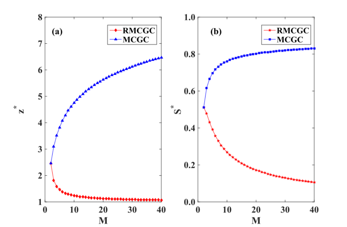
In Eq. (20), it is assumed that every replica node of a given node is damaged simultaneously (with probability ). On the contrary, in presence of redundant interdependencies it is natural to assume that the initial damage is inflicted to each replica node independently (with probability ). Therefore, in order to compare the robustness of the multiplex networks in presence and in absence of redundant interdependencies, we set , i.e., replica nodes are not initially damaged, and compare the critical value of the average degree at which the percolation transition occurs respectively for the RMCGC and for the MCGC. Additionally we will characterize also the size of the jump in the size of the RMCGC and the MCGC at the percolation transition. In Fig. 5, we display the values of and as a function of the number of layers for the RMCGC and the MCGC. For , the two models give the same results as they are identical. For , differences arise. In presence of redundant interdependencies, multiplex networks become increasingly more robust as the number of layers increases. This phenomenon is apparent from the fact that the RMCGC emerges for multiplex networks with an average degree of their layers which decreases as the number of layers increases. On the contrary, in ordinary percolation the value of for the emergence of the MCGC is an increasing function of . Additionally, the size of the discontinuous jumps at the transition point decreases with for the RMCGC, while increases with for the MCGC showing that the avalanches of failures have a reduced size for the RMCGC. We expect that the beneficial effect of the addition of new layers will extend also to the scenario in which the number of operating layers necessary for a node to be functional is assumed to be lager than two. Also, we believe that the same conclusion will apply to more general multilayer network structures where nodes have different number of interlinks (redundant interdependencies) such as a the topologies considered in Ref. [28] as long as the number of operating layers necessary for a node to be functional is the same for every node.
IV.3 Comparison with numerical simulations
In this section, we compare the results obtained with Eqs. (1), (2), (3), and (4) on a single instance of damage with the predictions the message-passing algorithm described in Eq. (13) characterizing the size of the RMCGC in an ensemble of networks. Specifically, we consider the case of a multilayer network with Poisson layers with the same average degree . In order to draw the percolation diagram for single instances of initial damage as a function of the probability of damage , we associate each replica node with a random variable drawn from a uniform distribution and we set
Fig. 6 displays the comparison between the two approaches, showing an almost perfect agreement between them.

Additionally in Fig. 7, we compare simulation results averaged over several realizations of the initial damage and several instances of the multiplex network model with the theoretical predictions given by the numerical solution of Eqs. (11)-(17), obtaining a very good agreement.

V MULTIPLEX NETWORKS WITH LINK OVERLAP
V.1 Link overlap, multilinks and multidegree
In isolated networks, two nodes can be either connected or not connected. In multiplex networks instead, the complexity of the structure greatly increases as the ways in which a generic pair of nodes can be connected is given by possibilities. A very convenient way of accounting for all the possibilities with a compact notation is to use the notion of multilink among pairs of nodes [16, 7]. Multilinks with , describe any of the possible patterns of connections between pairs of nodes in a multilayer network with layers. Specifically, indicates that a connection exists in layer , whereas indicates that the connection in layer does not exists. In particular, we can say that, in a multiplex network with layers, two nodes and are connected by the multilink
| (24) |
In order to distinguish the case in which two nodes are not connected in any layer with the case in which in at least one layer the nodes are connected, we distinguish between the trivial multilink and the nontrivial multilinks . The trivial multilink indicates the absence of any sort of link between the two nodes.
Using the concept of multilinks, one can define multiadjacency matrices whose element indicates whether () or not a node is connected to node by a multilink . The matrix elements of the multiadjacency matrix are given by
| (25) |
We note that multiadjacency matrices are essentially equivalent to rank-3 tensors as those considered in Ref. [15] for multiplex networks, and generalized to the case of arbitrary multilayer networks in Ref. [14]. Using multiadjacency matrices, it is straightforward to define multidegrees [16, 7]. The multidegree of node indicated as is the sum of rows (or columns) of the multiadjacency matrix , i.e.,
| (26) |
and indicates how many multilinks are incident to node .
Using a multidegree sequence , it is possible to build multiplex network ensembles that generalize the configuration model. This way, overlap of links is fully preserved by the randomization of the multiplex network. These ensembles are specified by the probability attributed to every multiplex network of the ensembles, where is given by
| (27) |
with normalization constant equal to the number of multiplex networks with given multidegree sequence.
V.2 General discussion of the message-passing equations for the RMCGC
Our goal here is to generalize the message-passing algorithm already given by Eqs. (1), (2), (3), and (4) for a generic single instance of a multiplex network and single realization of initial damage to the cases of (i) random multiplex networks with given multidegree sequence and/or (ii) random realizations of the initial damage. The extensions for both cases has been already considered for the case of multiplex networks without link overlap. In presence of link overlap, however, a more complex formalism is needed. For two nodes and in fact, the messages given by Eq. (1) and sent from node to node over the different layers are correlated because they all depend on the value of the variable given by Eq. (2). Such correlations require particular care when averaging the messages to treat the percolation transition for random initial damages. Similar technical challenges are also present in the treatment of the MCGC model where interdependencies are not redundant [37, 26]. In presence of redundant interdependencies there is an additional precaution that needs to be taken. In fact, the messages are explicitly dependent on the state of all replicas of node . This state is indicated by the variables where specifies whether the replica node is initially damaged or not. As a consequence of this property, when averaging over random realizations of initial damage, message-passing equations are written in terms of the messages explicitly accounting for the probability that node is sending to node the set of messages , given that node is in state and node and node are connected by a multilink . We have derived these equations for a general multiplex network with layers. However, the message-passing algorithm has a very long expression. To make the paper more readable, we decided to place the exact treatment of the general case in the SM, and consider here only the special case of ensembles of random multilayer networks with overlap. For these ensembles in fact, the message-passing equations are written in terms of average messages sent between nodes with given multilinks , i.e., , and the equations greatly simplify. Two specific cases of multilayer network ensembles are discussed below, for the cases of and layers.
V.3 Ensembles of multilayer networks link overlap and layers
In this case, every replica node is in the RMCGC if and only if also its interdependent node in the other layer is in the RMCGC. Therefore, the only messages that are different from zero are the messages sent to nodes in state . Specifically, we consider the case of a random multiplex network with Poisson multidegree distributions characterized by the averages
| (28) |
The messages only depend on the multiplicity of overlap of the multilinks and given respectively by
| (29) |
The fraction of replica nodes in the RMCGC is determined by the variables
| (30) |
where for example the value of indicates the probability that node to sends a message to its neighbor with connected by a multilink .
The values of the variables and are determined by the following set of equations (See Supplementary Material for details)
| (31) |
These equations are the same equations as those that determine the value of the MCGC as long we make the substitution [37, 26] taking into account that the damage in each replica node is independent in the present model. Notably in this case the percolation phase transition is discontinuous and hybrid been characterized by a square-root singularity above for approaching the percolation threshold from above.
V.4 Ensembles of multilayer networks link overlap and layers

We consider now the case of a random multiplex network with layers. The network has Poisson multidegree distributions and averages given by
| (32) |
In this case, the messages only depend on
| (33) |
Therefore the fraction of replica nodes in the RMCGC is determined by the variables
| (34) |
The equations that these variables need to satisfy can be described in a symbolic way by suitable diagrams (see the Supplementary Material for details in how to read these diagrams). Diagrams that describe the equations to determine the value of all the variables are presented in Fig. 8. These equations read as
| (35) |
where
| (36) |
We note that, in absence of overlap, i.e., for , and , Eqs. (SM38) reduce Eqs. (17).
By defining a suitable order of the variables , it is possible to introduce a vector whose elements are the variables , and rewrite the Eqs. (SM38) in a matrix form as
| (37) |
The hybrid discontinuous phase transition (characterized by a square root singularity) can be found by imposing that the system of Eqs. (37) is satisfied together with the condition that the determinant of the Jacobian of equals to zero, that is
| (38) |
Simulation results of the percolation process for multiplex networks in this ensemble are presented in Fig.9, and they provide clear evidence of a perfect agreement to the theoretical prediction.

VI Conclusions
In this paper, we introduced and fully characterized an alternative percolation model for multiplex networks. The model serves to quantify the robustness of networks with redundant interdependencies. According to the model, interdependencies make a system more fragile than it would be by considering each layer independently. This fact is consistent with the original model used to study percolation in multiplex networks [4, 23, 21], and it is apparent from the fact that the transition is abrupt for any number of network layers considered in the interdependent model. On the other hand, redundancy of interdependencies across multiple layers favors system robustness, as the height of the discontinuous jump and the location of the transition point decrease as the number of layers increases. This is a fundamental difference with respect to the model currently adopted to study the robustness of multiplex networks and multilayer network in general, where instead increasing the number of layers generates more and more fragile networks [23, 26, 27, 28].
To characterize the model, we deployed a comprehensive theoretical approach based on message passing. Our theory is valid for arbitrary multiplex network topologies as long as they are locally treelike. The theory is further developed in the context of ensembles of synthetic network models to analyze properties of the percolation transition emerging in the new model, and to perform systematic comparisons, and emphasize fundamental differences, with the percolation model introduced in Ref. [4].
We remark that ours is not a definitive model, but it represents only a good starting point towards a more realistic description of real multiplex systems. For instance, we do not expect to observe a qualitative change of the results if the redundancy is weaker and let us say a node is damaged only if less than two interdependent nodes are functioning. However, our approach is purely structural and in many situations, forgetting about intrinsic dynamical features may be not appropriate. The primary role of our model is to emphasize the importance of redundancy or complementarity in multilayer networks, an obvious-yet-neglected feature of many real systems. In several realistic settings in fact, system robustness is augmented by the addition of new layers of interactions, as these layers are indeed created to provide backup options. For example, adding a new mode of transportation in a preexisting multimodal transportation system should make the system more reliable against eventual failures. Similarly in a living organism, the development of new types of interactions among constituents should increase the stability of the same organism against possible mutations. In the current setting, the model assumes that the functioning of individual nodes requires that nodes are correctly operating on at least two interdependent layers. The model can be, however, generalized to deal with a variable number of minimal functioning layers to describe more realistic scenarios in specific situations of interest.
Acknowledgements.
F.R. acknowledges support from the National Science Foundation (CMMI-1552487) and the U.S. Army Research Office (W911NF-16-1-0104).References
- [1] S. Boccaletti, G. Bianconi, R. Criado, C. I. del Genio, J. Gómez-Gardeñes, M. Romance, I. Sendiña-Nadal, Z. Wang, and M. Zanin, The structure and dynamics of multilayer networks, Phys. Rep. 544, 1 (2014).
- [2] M. Kivelä, A. Arenas, M. Barthélemy, J. P. Gleeson, Y. Moreno, and M. A. Porter, Multilayer Networks, J. Complex Netw. 2, 203 (2014).
- [3] K.-M. Lee, B. Min, and K.-I. Goh, Towards real-world complexity: an introduction to multiplex networks, Eur. Phys. Jour. B 88, 1 (2015).
- [4] S. V. Buldyrev, R. Parshani, G. Paul, H. E. Stanley and S. Havlin, Catastrophic cascade of failures in interdependent networks, Nature 464, 1025 (2010).
- [5] J. Gao, S. V. Buldyrev, H. E. Stanley, and S. Havlin, Networks Formed from Interdependent Networks, Nat. Phys. 8, 40 (2012).
- [6] M. Szell, R. Lambiotte, and S. Thurner, Multirelational organization of large-scale social networks in an online world, Proc. Natl. Acad. Sci. USA 107, 13636 (2010).
- [7] G. Menichetti, D. Remondini, P. Panzarasa, R. J. Mondragón, and G. Bianconi, Weighted multiplex networks, PloS one 9, e97857 (2014).
- [8] A. Cardillo, J. Gómez-Gardeñes, M. Zanin, M. Romance, D. Papo, F. del Pozo, and S. Boccaletti, Emergence of network features from multiplexity, Sci. Rep. 3, 1344 (2013).
- [9] M. De Domenico, A. Solé-Ribalta, S. Gómez, and A. Arenas, Navigability of interconnected networks under random failures, Proc. Natl. Acad. Sci. USA 111, 8351(2014).
- [10] V. Nicosia and V. Latora, Measuring and modeling correlations in multiplex networks, Phys. Rev. E 92, 032805 (2015).
- [11] J. Menche, A. Sharma, M. Kitsak, S. D. Ghiassian, M. Vidal, J. Loscalzo and A.-L. Barabási, Uncovering disease-disease relationships through the incomplete interactome, Science 347, 1257601 (2015).
- [12] E. Bullmore and O. Sporns, Complex brain networks: graph theoretical analysis of structural and functional systems, Nat. Rev. Neurosci. 10, 186 (2009).
- [13] S. D. S. Reis, Y. Hu, A. Babino, J. S. Andrade Jr., S. Canals, M. Sigman and H. A. Makse, Avoiding catastrophic failure in correlated networks of networks, Nature Phys. 10, 762 (2014).
- [14] M. De Domenico, A. Solé-Ribalta, E. Cozzo, M. Kivelä, Y. Moreno, M. A. Porter, S. Gómez and A. Arenas, Mathematical formulation of multilayer networks, Phys. Rev. X 3, 041022 (2013).
- [15] P.J. Mucha, T. Richardson, K. Macon, M.A. Porter and J.P. Onnela, Community Structure in Time-Dependent, Multiscale, and Multiplex Networks, Science 328, 876 (2010).
- [16] G. Bianconi, Statistical mechanics of multiplex networks: Entropy and overlap, Phys. Rev. E 87, 062806 (2013).
- [17] N. Azimi-Tafreshi J. Gómez-Gardeñes and S. N. Dorogovtsev, k-core percolation on multiplex networks, Phys. Rev. E 90, 032816 (2014).
- [18] G.J. Baxter, S.N. Dorogovtsev, J.F. F. Mendes and D. Cellai, Weak percolation on multiplex networks, Phys. Rev. E 89, 042801 (2014).
- [19] A. Hackett, D. Cellai, S. Gómez, A. Arenas and J. P. Gleeson, Bond Percolation on Multiplex Networks, Phys. Rev. X 6, 021002 (2016).
- [20] S. Watanabe and Y. Kabashima, Cavity-based robustness analysis of interdependent networks: Influences of intranetwork and internetwork degree-degree correlations, Phys. Rev. E. 89, 012808 (2014).
- [21] G. J. Baxter, S. N. Dorogovtsev, A. V. Goltsev and J. F. F. Mendes, Avalanche collapse of interdependent networks, Phys. Rev. Lett. 109, 248701 (2012).
- [22] B. Min, S. D. Yi, K.-M. Lee and K.-I. Goh, Network robustness of multiplex networks with interlayer degree correlations, Phys. Rev. E 89, 042811 (2014).
- [23] S.-W. Son, G. Bizhani, C. Christensen, P. Grassberger and M. Paczuski, Percolation theory on interdependent networks based on epidemic spreading, EPL 97, 16006 (2012).
- [24] R. Parshani, C. Rozenblat, D. Ietri, C. Ducruet and S. Havlin, Inter-similarity between coupled networks, EPL 92, 68002 (2010).
- [25] R. Parshani, S. V. Buldyrev and S. Havlin, Interdependent networks: Reducing the coupling strength leads to a change from a first to second order percolation transition, Phys. Rev. Lett. 105, 048701 (2010).
- [26] D. Cellai, S.N. Dorogovtsev and G.Bianconi, Message passing theory for percolation models on multiplex networks with link overlap, Phys. Rev. E 94, 032301 (2016).
- [27] G. Bianconi, S. N. Dorogovtsev and J. F. F. Mendes, Mutually connected component of networks of networks with replica nodes, Phys. Rev. E 91, 012804 (2015).
- [28] G. Bianconi and S. N. Dorogovtsev, Multiple percolation transitions in a configuration model of a network of networks, Phys. Rev. E 89, 062814 (2014).
- [29] F. Radicchi and A. Arenas, Abrupt transition in the structural formation of interconnected networks, Nature Phys. 9, 717–720 (2013).
- [30] E. Leicht and R. D’Souza, Percolation on interacting networks, arXiv:0907.0894 (2009) .
- [31] K.-M. Lee, J.Y. Kim, W. Cho, K.-I. Goh and I-M. Kim, Correlated multiplexity and connectivity of multiplex random networks, New J. Phys. 14, 033027 (2012).
- [32] J. Shao, S. V. Buldyrev, S. Havlin, and H. E. Stanley, Cascade of Failures in Coupled Network Systems with Multiple Support-Dependence Relations, Phys. Rev. E 83, 036116 (2011).
- [33] S. N. Dorogovtsev, A. Goltsev and J. F. F. Mendes, Critical phenomena in complex networks, Rev. Mod. Phys. 80, 1275 (2008).
- [34] B. Karrer, M. E. J. Newman, and L. Zdeborová, Percolation on sparse networks, Phys. Rev. Lett. 113, 208702 (2014).
- [35] M. Mezard and A. Montanari, Information, Physics and Computation (Oxford University Press, Oxford, 2009).
- [36] A. K. Hartmann and M. Weigt, Phase Transitions in Combinatorial Optimization Problems, (WILEY-VCH, Weinheim, 2005).
- [37] G. J. Baxter, G. Bianconi, R. A. da Costa, S. N. Dorogovtsev and J. F. F. Mendes, Correlated link overlaps in Multiplex Networks, Phys. Rev. E 94, 012303 (2016).
- [38] D. Cellai, E. López, J. Zhou, J. P. Gleeson and G. Bianconi, Percolation in multiplex networks with overlap, Phys. Rev. E 88, 052811 (2013).
- [39] F. Radicchi, Percolation in real interdependent networks, Nature Phys. 11, 597 (2015).
- [40] B. Min, S. Lee, K.-M. Lee, and K-I. Goh, Link overlap, viability, and mutual percolation in multiplex networks, Chaos, Solitons & Fractals 72 49 (2015).
- [41] F. Radicchi and C. Castellano, Beyond the locally treelike approximation for percolation on real networks, Phys. Rev. E 93, 030302(R) (2016).
- [42] S. Gómez, A. Díaz-Guilera, J. Gómez-Gardeñes, C. J. Perez-Vicente, Y. Moreno and A. Arenas, Diffusion dynamics on multiplex networks, Phys. Rev. Lett. 110, 028701 (2013).
- [43] M. De Domenico, C. Granell, M. A. Porter and A. Arenas, The physics of spreading processes in multilayer networks, Nature Phys. 12, 901–906 (2016).
- [44] J. Gao, S. V. Buldyrev, S. Havlin, and H. E. Stanley, Robustness of a Network Formed by n Interdependent Networks with a One-to-One Correspondence of Dependent Nodes, Phys. Rev. E 85, 066134 (2012).
- [45] J. Gao, S. V. Buldyrev, S. Havlin, and H. E. Stanley, Robustness of a Network of Networks, Phys. Rev. Lett. 107, 195701 (2011).
SUPPLEMENTAL MATERIAL
SM0.1 Message passing for given multilayer network and given initial damage
Let us consider a given multilayer network with layers. Each layer of the multilayer network has adjacency matrix . In this multilayer network, each pair of nodes and is connected by a multilink
| (SM1) |
Any two nodes and are connected by a nontrivial multilink is implying that at least one link between the two nodes is present across the layers. We assume that the initial damage configuration is known and that it is given by the set of variables where indicates if a replica is initially damaged () or not (). The message-passing algorithm given in Sec. III of the main text allows us to determine for any given initial damage configuration, if any replica node is in the RMCGC () or not () as long as the multilayer network is locally treelike. Specifically the variables are determined in terms the set of messages
| (SM2) |
going from any node to any node joined by a nontrivial multilink .
The messages are determined according to the following recursive equation
| (SM3) |
where indicates the set of nodes that are neighbor of node in layer and where is the step function with values for and for . Here the variable indicates in how many layers node is connected to the RMCGC assuming that node also belongs to the RMCGC,
| (SM4) |
Finally the variables are expressed in terms of the messages and are given by
| (SM5) |
In many situations, however, the initial configuration of the damaged is not known, and instead it is only known the probability distribution of the initial damage configuration.
In this case, one aims to know the probability that a replica node is in the RMCGC for a random configuration of the initial damage. The value of , on a locally treelike multilayer network is determined by a distinct message-passing algorithm that can be derived from the message-passing algorithm valid for single realization of the initial damage, by performing a suitable average of the messages.
Particular care should be taken when one aims to perform this average. In fact depends on all the messages sent by node to node in all the layers . These messages are correlated and therefore they cannot be averaged independently.
An alternative formulation of the Eqs. provides the necessary framework for deriving in few steps the message-passing algorithm to predict . This alternative formulation is written terms of the variables indicating whether () or not () node send to node a message given that node is connected to node by a multilink .
Using Eqs. it is easy to see that the value of the variables is determined by the following equations:
- (a)
if and ,
(SM6) - (b)
if and ,
(SM7) - (c)
if and ,
(SM8)
where is determined in terms of the messages as
| (SM9) |
Finally a replica node is in the RMCGC () or not () depending on the messages it receives from its neighbors, i.e.
| (SM10) |
SM0.2 Message-passing algorithm for random damage
By averaging Eqs. we can derive the message-passing algorithm predicting the probability that a replica node is in the RMCGC when the initial damage is randomly drawn for the probability distribution . Assuming that each replica node is damaged independently the probability distribution is given by
| (SM11) |
The message-passing algorithm valid for a random distribution of the initial disorder, is written in terms of the messages . The messages take real values between zero and one. They indicate the probability that node send to node a message given that node is connected to node by a multilink and that node has initial damage configuration , i.e. .
Let us indicate with the probability of a local initial damage configuration given by
| (SM12) |
and let us indicate with the vector
| (SM13) |
of elements . Using this notation, the messages are determined by the following algorithm (see last section of this Supplementary Information for the derivation of these results):
- (a)
if and ,
(SM14) where
(SM15) - (b)
if , and ,
(SM16) - (c)
if and ,
(SM17)
Finally the probability that a replica node is in the RMCGC is given by
| (SM18) | |||||
SM0.3 Average over multilayer ensemble with give multidegree sequence
In order to derive the phase diagram of the percolation transition in presence of redundant interdependencies over given multilayer network ensembles, it is useful to consider a further average of the messages . To this end we consider the multilayer network ensemble that preserves the multidegree sequence . Every multilayer network in this ensemble has probability
| (SM19) |
where is a normalization constant equal to the number of multilayer networks with the given multidegree sequence.
In this multilayer network ensemble the average messages indicate the probability that a message is sent toward a node with initial damage configuration over a multilink . These average messages can be found by solving the following recursive equations:
- (a)
if
(SM20) where
(SM21) - (b)
if ,
(SM22) - (c)
if
(SM23)
Finally the probability that a replica node in layer is in the RMCGC in the multilayer network ensemble is given by
| (SM24) | |||||
SM0.4 Derivation of Eq.
In this section, we will discuss in detail the derivation of Eq. from Eq.(SM6). A similar derivation (that we omit here) can be performed to derive Eqs. from Eqs. .
We start from Eq. (SM6) written for the messages sent from a node to a node with satisfying and . This equation is rewritten here for convenience,
| (SM25) |
We given a set of variables we can use the following identity
| (SM26) |
where in the last expression we perform a sum over all the -dimensional vectors
| (SM27) |
with if and if . Using this expansion for the products in Eq. we obtain
| (SM28) |
where is given by Eq. . By using the fact that the messages take only values zero or one, that that out of all the messages from node to node only one is actually equal to one, and all the others are zero, we can rewrite Eq. as
| (SM29) |
Finally, averaging over the probability distribution of the configuration of the initial damage of node , in the locally treelike approximation we obtain for the messages the Eq. that we rewrite here for convenience,
| (SM30) | |||||
SM0.5 Ensembles of multilayer networks link overlap and layers
In the multilayer network case with and link overlap, every replica node is in the RMCGC if and only if also its interdependent node in the other layer is in the RMCGC. Therefore, the only messages that are different from zero are the messages sent to nodes in state . Specifically, we consider the case of a random multilayer network with Poisson multidegree distributions characterized by the averages
| (SM31) |
The messages only depend on the multiplicity of overlap of the multilinks and given respectively by
| (SM32) |
The fraction of replica nodes in the RMCGC is determined by the variables
| (SM33) |
The value of indicates the probability that node to sends a message to its neighbor with connected by a multilink . This fact occurs if and only if node has both replica nodes that are not initially damaged (which occurs with probability ) and if at least one positive message in each layer is reaching node from neighbors different from . The value of indicates the probability that node sends a message to its neighbor with connected by a multilink or equivalently sends a message to its neighbor with connected by a multilink . This fact occurs if and only if node has both replica nodes that are not initially damaged (which occurs with probability ) and if at least one positive message in each layer is reaching node from neighboring nodes different from . The latter is a necessary condition to have . The value indicates the probability that node is sending a message to its neighbor in state and connected by a multilink or equivalently sends a message to its neighbor in state and connected by a multilink . This fact occurs if only if node has both replica nodes that are not initially damaged (which occurs with probability ) and if at least one positive message is reaching node in the layer for which from neighbors different from and no positive message is reaching node in the layer where from neighboring nodes different from node . Finally, is the probability that a replica node is in the RMCGC which implies that (i) it is not initially damaged, (ii) its replica node in the other layer is not initially damaged, and (iii) at least one positive message reaches node in both layers.
The values of the variables and are therefore determined by the following set of equations
| (SM34) |
SM0.6 Ensembles of multilayer networks link overlap and layers
Let us consider the case of a random multilayer network with layers with Poisson multidegree distributions and averages given by
| (SM35) |
In this case, the messages only depend on the multiplicity of overlap of the multilinks and and the number of layers where and . Therefore, messages depend only on
| (SM36) |

The fraction of replica nodes in the RMCGC is determined by the variables
| (SM37) |

Let us explicitly describe the equations that one of these variables needs to satisfy, and introduce a symbolic way to describe the equations. Specifically, we consider as the probability that a node , connected to a node by a multilink , sends to node a message provided that node is in the state (see Fig. SM1). This probability is equal to the sum of (i) the probability that node is in the state [which occurs with probability ] and it sends the message to node and (ii) the probability that node is in the state (which occur with probability ) and sends the same message to node . Node sends the message only if the following conditions are met:
- (i)
if node is in the state , node must receive at least one positive message from nodes different from node in layers and .
- (ii)
if node is in the state , node must receive at least one positive message from nodes different from node in layers and and must not receive any positive message from nodes different from node in layer .
These requirements are summarized by the diagram of Fig. SM1. Diagrams that describe the equations to determine the value of all the other variables are presented in Fig. SM2. These equations read as
| (SM38) |
where
| (SM39) |
In the main text we compared the result of these equation with simulation results of the percolation process in this ensemble of multiplex networks averaged over different multiplex network realizations. Here for completeness we also show simulation results of the percolation process on a single instance of multiplex network and given initial damage in this ensemble with the results of the message-passing algorithm proposed in Sec. III of the main text (see figure SM3).
