The Final SDSS High-Redshift Quasar Sample of 52 Quasars at Facilities: Bok (90Prime), MMT (SWIRC, Red Channel Spectrograph), Hale (DBSP), LBT (MODS), Gemini:North (GNIRS), Magellan:Baade (FIRE), SDSS
Abstract
We present the discovery of nine quasars at identified in the Sloan Digital Sky Survey (SDSS) imaging data. This completes our survey of quasars in the SDSS footprint. Our final sample consists of 52 quasars at , including 29 quasars with mag selected from 11,240 deg2 of the SDSS single-epoch imaging survey (the main survey), 10 quasars with selected from 4223 deg2 of the SDSS overlap regions (regions with two or more imaging scans), and 13 quasars down to mag from the 277 deg2 in Stripe 82. They span a wide luminosity range of . This well-defined sample is used to derive the quasar luminosity function (QLF) at . After combining our SDSS sample with two faint ( mag) quasars from the literature, we obtain the parameters for a double power-law fit to the QLF. The bright-end slope of the QLF is well constrained to be . Due to the small number of low-luminosity quasars, the faint-end slope and the characteristic magnitude are less well constrained, with and mag. The spatial density of luminous quasars, parametrized as , drops rapidly from to 6, with . Based on our fitted QLF and assuming an IGM clumping factor of , we find that the observed quasar population cannot provide enough photons to ionize the IGM at % confidence. Quasars may still provide a significant fraction of the required photons, although much larger samples of faint quasars are needed for more stringent constraints on the quasar contribution to reionization.
Keywords:
galaxies: active — galaxies: high-redshift — quasars: general — quasars: emission linesI Introduction
High-redshift () quasars are a powerful tool to study the early universe. In recent years, more than 100 quasars at have been discovered. The Sloan Digital Sky Survey [120, SDSS;] pioneered the searches of quasars at these redshifts, followed by the Canada-France High-redshift Quasar Survey [111, CFHQS;], the UKIRT Infrared Deep Sky Survey [109, UKIDSS;], and the Panoramic Survey Telescope & Rapid Response System 1 [60, Pan-STARRS1;] survey. To date over 40 quasars have been discovered based on the SDSS imaging data [25, 27, 28, 29, 52, 53, 56, e.g.]. The UKIDSS has discovered several quasars [100, 79, 80], including the most distant quasar known at [80, 7]. The CFHQS found 20 quasars over deg2 of sky [111, 112, 114]. The Pan-STARRS1 covers 3 steradians of the sky, and is now producing a large number of high-redshift quasars [78, 4, 102, 6], including three quasars at [102]. Most recently, the VISTA Kilo-Degree Infrared Galaxy (VIKING) survey, the Dark Energy Survey (DES), the VST ATLAS survey, and the Subaru High- Exploration of Low-Luminosity Quasars (SHELLQ) project, have started to yield quasars [101, 17, 87, 71, e.g.]. The number of high-redshift quasar discoveries is increasing steadily.
Meanwhile, the sample of bright high-redshift quasars, especially luminous SDSS quasars, have been studied extensively in multiple wavelength bands from X-ray to radio. These quasars are very luminous with mag. Deep optical spectra have revealed strong or even complete absorption in the Ly forests, indicating that the redshift probed () is close to the epoch of cosmic reionization [8, 110, 30, 15, 12, 74, e.g.]. Their infrared spectroscopy show that these luminous quasars harbor billion-solar-mass black holes and emit near the Eddington limit, suggesting the rapid growth of central black holes at this early epoch [51, 63, 113, 21, 58, 116, e.g.]. The broad emission lines of these quasars exhibit solar or supersolar metallicity, implying that vigorous star formation and element enrichment have occurred in their broad-line regions [51, 57, 20, e.g.]. In addition, observations in the mid/far-IR, mm/sub-mm, and radio wavebands have provided rich information about the dust emission and star formation in the host galaxies [50, 54, 103, 35, 106, 107, 16, 82, 14, 65, 5, 67, e.g.]. Therefore, high-redshift quasars are a powerful probe for understanding black hole accretion, galaxy evolution, and the intergalactic medium (IGM) state in the first billion years of cosmic time.
In this paper, we present nine quasars newly found in the SDSS, including seven quasars in the SDSS main survey area, one quasar in the SDSS overlap regions, and one quasar in SDSS Stripe 82. The overlap regions are the regions with overlapping imaging in the SDSS, which results in multiple observations of individual sources within these regions. Stripe 82 covers deg2, and was repeatedly scanned 70–90 times by the SDSS imaging survey. We describe these regions in Section 2. With the discovery of these nine quasars, we have completed our survey of quasars in the SDSS footprint. We summarize our survey of SDSS quasars in the second half of the paper. With a total of 52 quasars, we derive the quasar luminosity function (QLF) at , and in particular, improve the measurement of the QLF at the bright end.
The layout of the paper is as follows. In Section 2, we review our survey of quasars in the SDSS. In Section 3, we present the nine new quasars. In Section 4, we summarize our complete sample of 52 SDSS quasars and calculate the QLF at . In Section 5, we discuss the evolution of luminous quasars at high redshift and the quasar contribution to cosmic reionization at . We summarize the paper in Section 6. Throughout the paper, SDSS magnitudes are expressed in the AB system. Near-IR and mid-IR magnitudes are in the Vega system. We use a -dominated flat cosmology with km s-1 Mpc-1, , and .
II Survey of quasars in the SDSS
In this section, we briefly review our survey of quasars selected in the SDSS. We will need this information for Sections 3 and 4. The SDSS is an imaging and spectroscopic survey of the sky using a dedicated wide-field 2.5 m telescope [42] at Apache Point Observatory. Imaging was carried out in drift-scan mode using a 142 mega-pixel camera [41] which gathered data in five broad bands, , spanning the range from 3000 to 10,000 Å [38], on moonless photometric [45] nights of good seeing. The effective exposure time was 54.1 seconds. An SDSS run (strip) consists of 6 parallel scanlines (camera columns) for each of the five bands. The scanlines are wide with gaps of roughly the same width, so two interleaving strips make a stripe. SDSS scanlines are divided into fields, and a field is the union of five frames covering the same region of sky. The images were processed using specialized software [66], and are photometrically [99, 48, 83] and astrometrically [85] calibrated using observations of a set of primary standard stars [97] on a neighboring 20-inch telescope.
II.1 Quasars in the SDSS Main Survey
The initial goal of the SDSS imaging survey was to scan 8500 deg2 of the north Galactic cap. The total unique area was expanded to 14,555 deg2, by adding 5000 deg2 in the south Galactic cap (SGC) [2]. Fan et al. [25], Fan et al. [27], Fan et al. [28], Fan et al. [29] discovered 19 quasars from the SDSS photometry, primarily in the north Galactic cap. Most of these quasars are bright ( mag), and were selected from single-epoch imaging data (hereafter referred to as the SDSS main survey). They represent the most luminous quasars at . However, there were main survey regions remaining unsearched, particularly in the SGC. In this paper we report on the discovery of additional quasars found in these regions.
The quasar selection procedure in the main survey has been discussed in detail in the papers mentioned above. Here we briefly review the procedure. Because of the rarity of high-redshift quasars and overwhelming number of contaminants, the procedure consists of four basic steps. The first step is to select -band dropout objects mainly in high galactic latitude . Sources with mag and -band error mag (roughly mag) that were not detected in the bands are selected as -dropout objects. The simple color cut is used to separate quasars (and cool brown dwarfs) from the majority of stellar objects [23, 98, e.g.]. Beyond the limit of mag, the number of contaminants increases dramatically. The second step is to remove false -dropout objects and improve photometry. All -dropout objects are visually inspected, and false detections such as cosmic rays are removed. If necessary, we also take deeper imaging data to improve the and -band photometry to reduce the number of contaminants. The third step is to take near-IR (usually band) photometry of -dropout objects with another telescope. In the versus color-color diagram, high-redshift quasar candidates are separated from brown dwarfs. Specifically, quasar candidates satisfy the criterion (see also Figure 1). The final step is to take spectroscopic observations and identify quasar candidates.

In addition to the above ‘standard’ survey to a limit of detections in the SDSS -band images, we also selected two small samples of quasar candidates using a ‘non-standard’ method. The first sample consisted of candidates down to in the -band images in part of the UKIDSS footprint. This is similar to the test done by Fan et al. [29]. We used a more stringent color cut mag to reduce the number of contaminants caused by larger photometric uncertainties. We further required that the candidates should be detected at a significance level of in the UKIDSS and bands. Two of the quasars in this paper were selected using this method. The second ‘non-standard’ sample consisted of several candidates with colors between 2.1 and 2.2 mag, slightly bluer than that used for the ‘standard’ survey. One quasar in this paper was selected using this method.
II.2 Quasars in the SDSS Stripe 82
In addition to the single-epoch main imaging survey, the SDSS also conducted a deep survey by repeatedly imaging a deg2 area on the Celestial Equator in the south Galactic cap [1, 3, 55]. This deep survey stripe, or Stripe 82, roughly spans and , and was scanned 70–90 times in total, depending on R.A. along the stripe. The multi-epoch data have been used to construct co-added images that can reach two magnitudes deeper than the SDSS single-epoch images [3, 55, 34, e.g.]. Using these co-added data, we have found 12 quasars in Stripe 82 [52, 53]. These quasars have mag, and are on average two magnitudes fainter than those found in the main survey. In this paper we present one new quasar found in Stripe 82. The quasar selection procedure for Stripe 82 is very similar to that for the main survey, except that the survey limit is mag ( mag) instead of mag.
II.3 Quasars in the SDSS Overlap Regions
We have also carried out searches of quasars in the SDSS overlap regions, the regions that were scanned by two or more SDSS imaging runs. The SDSS imaging runs generally overlap each other, due to the survey geometry and strategy. The imaging survey in drift-scan mode was along great circles, and had two common poles. The fields overlap more substantially when they approach the survey poles. In addition, the two interleaving strips that make any stripe overlap slightly, leading to repeat observations in a small area. Furthermore, if the quality of a run, or part of a run, did not meet the SDSS standard seeing and photometric criteria, the relevant region was re-observed, yielding duplicate observations in this region. The total area of the overlap regions is more than one-fourth of the SDSS footprint. These overlap regions provide a unique dataset that allows us to select high-redshift quasars more than 0.5 mag fainter (in the band) than those found with the SDSS single-epoch data. We have discovered eight quasars in the overlap regions [56].
The selection procedure of overlap-region quasars is slightly different from those described above. The image quality is usually different between the repeat runs. In the first step of the selection procedure, the magnitude limit for both ‘primary’ and ‘secondary’ detections is mag or mag ( detection). The candidates are actually fainter than detections, because otherwise they would have been selected in the main survey. We focused on high galactic latitude () regions. Using repeat observations ensures that most -dropout objects we select are physical sources, rather than artifacts or cosmic rays. In the second step, we take deeper and band images to improve photometry for -dropout objects. The rest of the selection procedure remains the same. The details are given in Jiang et al. [56].
III Discovery of nine new quasars
In this section we present the discovery of nine new quasars in the SDSS. The basic information of the quasars, including their coordinates, redshifts, and broad-band () photometry, is given in Table 1. One of them (SDSS J083525.76+321752.6; hereafter we use J0835+3217 for brevity) is found in the overlap regions, and another one SDSS J211951.89–004020.1 (hereafter J2119–0040) is found in Stripe 82. The other seven quasars were found based on the SDSS single-epoch data. The naming convention for SDSS sources is SDSS JHHMMSS.SSDDMMSS.S, and the positions are expressed in J2000.0 coordinates. For brevity, we use JHHMMDDMM in the following text.
| Quasar (SDSS) | Redshift | Notes | |||
|---|---|---|---|---|---|
| J081054.32+510540.1 | 5.80±0.03 | 21.52±0.13 | 19.34±0.07 | 18.77±0.06 | See also Bañados et al. [6] |
| J083525.76+321752.6 | 5.89±0.03 | ¿23.0 | 20.73±0.20 | 20.50±0.20 | Overlap regions |
| J114338.34+380828.7 | 5.81±0.03 | 21.97±0.19 | 19.76±0.09 | 18.98±0.09 | See also Bañados et al. [6] |
| J114803.28+070208.3 | 6.339±0.001 | 23.20±0.35 | 20.79±0.10 | 19.36±0.11 | See also S. Warren et al. (in prep.) |
| J124340.81+252923.9 | 5.85±0.03 | 23.08±0.29 | 20.22±0.10 | 19.21±0.12 | See also S. Warren et al. (in prep.) |
| J160937.27+304147.7 | 6.16±0.03 | ¿22.5 | 20.26±0.13 | 19.39±0.14 | See also S. Warren et al. (in prep.) |
| J162100.92+515548.8 | 5.71±0.03 | 21.86±0.13 | 19.70±0.07 | 19.11±0.20 | |
| J211951.89004020.1 | 5.87±0.03 | 23.99±0.27 | 21.68±0.10 | 20.87±0.12 | Stripe 82 |
| J231038.88+185519.7 | 6.003±0.001 | 21.66±0.25 | 19.21±0.09 | 17.94±0.05 |
III.1 Observations and Data Reduction
We first present the observations of quasar candidates in Stripe 82, which were done in 2009 and 2010. The -band photometry of -dropout objects (quasar selection procedure step 3) was made using the SAO Widefield InfraRed Camera [13, SWIRC;] on the MMT. The observing strategy is the same as that of Jiang et al. [52], Jiang et al. [53]. The observing conditions were typical, with relatively clear skies and seeing. The images were reduced using standard IRAF11 1 IRAF is distributed by the National Optical Astronomy Observatory, which is operated by the Association of Universities for Research in Astronomy (AURA) under cooperative agreement with the National Science Foundation. routines. We used bright UKIDSS or 2MASS [96] point sources in the same images for flux calibration. Based on the -band photometry, the final sample of quasar candidates was selected. We then used the MMT Red Channel Spectrograph [91, RCS;] to identify these candidates. The exposure time for each target was 20–30 minutes, depending on the object brightness and weather conditions. If a target was identified as a quasar, several further exposures were taken to improve the spectral quality. The MMT RCS data were reduced using standard IRAF routines.
The observations of quasar candidates in the SDSS overlap regions were conducted in 2015 and 2016. Deeper and -band photometry of -dropout objects (quasar selection procedure step 2) was made using the wide-field optical imager 90Prime on the 2.3m Bok telescope. The 90Prime images were reduced in a standard fashion using our own IDL routines. The details of the Bok observations and data reduction can be found in Jiang et al. [56]. For the -band photometry, we used the UKIDSS data for any candidates that have significant ( in ) detections in the UKIDSS. For the other candidates, we obtained their -band photometry using the MMT SWIRC. We used the MMT RCS and the Double Spectrograph (DBSP) on the Hale 5.1m telescope to identify quasar candidates and obtain high-quality optical spectra. The Hale DBSP data were reduced using standard IRAF routines as well.
The observations of quasar candidates in the SDSS main survey were done between 2010 and 2015, except for J1621+5155, which was observed in 2006. We used the Bok/90Prime to improve the and -band photometry for the sample of -dropout objects with mag. For the -dropout objects with mag, we simply used the SDSS data. The -band photometry was made using the MMT SWIRC, or from the UKIDSS archive for the objects detected at in the band. We then used the MMT RCS and the Hale DBSP to identify quasar candidates and obtain high-quality optical spectra, as we did for the candidates in the overlap regions. In addition, we took a deep optical spectrum for J2310+1855 in long slit mode using the Multi-Object Double Spectrograph (MODS) on the Large Binocular Telescope (LBT). The MODS spectra were reduced using standard IRAF routines.
We also obtained deep near-IR spectra for two quasars, J2310+1855 and J1148+0702, using Gemini GNIRS and Magellan FIRE, respectively. The GNIRS observation of J2310+1855 is part of our large Gemini GNIRS campaign of quasars (GN-2015B-LP-7). The GNIRS campaign is used to measure the rest-frame properties of a large sample of quasars, including UV continuum slopes, broad emission line properties, black hole masses and mass function, etc. Both GNIRS and FIRE (in echelle mode) provide a simultaneous wavelength coverage of m in cross-dispersion mode. The observing strategies for the two observations were the same. We used the standard ABBA nodding sequence between exposures. The exposure time at each nod position was 5 minutes, and the distance between the two positions was . Before or after the exposure of each quasar, a nearby A or F spectroscopic standard star was observed for flux calibration and to remove telluric atmosphere absorption. The GNIRS spectra were reduced using the IRAF Gemini package, and the details can be found in Jiang et al. [51]. The FIRE spectra were reduced using an IDL pipeline developed by the FIRE instrument team, and the details can be found in Simcoe et al. [95].
III.2 Results
From the above observations, we took spectra for about 30 candidates, and identified nine quasars, including one quasar (J0835+3217) in the SDSS overlap regions, one quasar (J2119–0040) in Stripe 82, and seven quasars in the main survey. Table 1 lists the coordinates, redshifts, and the broad-band photometry of the quasars. Column 1 shows the J2000 coordinates, or the source names. Column 2 shows the redshifts, which span the range . The redshifts were mostly measured from the Ly emission lines, or from the wavelength where the sharp flux decline occurs. The measurements can be slightly biased towards higher redshifts due to the Ly forest. The redshift error of 0.03 quoted in Column 2 is simply the scatter in the relation between Ly redshifts and systemic redshifts at low redshift [92, e.g.]. The uncertainties from our fitting process and wavelength calibration are negligible in comparison. The redshift of J1148+0702 is measured from its Mg ii emission line (see Section 3.2.1). The redshift of J2310+1855 is measured from the CO (6–5) observations by Wang et al. [107]. Columns 3 through 5 show the , , and -band photometry. The and -band photometry was taken from the SDSS, or improved by the Bok 90Prime. The -band photometry was taken from the UKIDSS, or obtained from the MMT SWIRC. These quasars span a brightness range of and a luminosity range of mag.
Among the seven quasars found in the main survey area, three quasars were selected using the ‘non-standard’ method mentioned in Section 2.1. J1148+0702 and J1609+3041 are fainter than a detection in the SDSS -band images, and J1621+5155 has an color slightly bluer than the 2.2 mag limit. Two quasars, J0810+5105 and J1143+3808, in Table 1, were independently discovered by the Pan-STARRS1 [6], as indicated in the last column. In addition, J1148+0702, J1243+2529, and J1609+3041 were independently discovered by the UKIDSS (S. Warren et al., in preparation; see also Mortlock [81]). We also recovered J0100+2802 at discovered by Wu et al. [116], and two quasars, J1545+6028 at and J2325+2628 at , found by F. Wang et al. [104]. We missed J2356–0622 at in F. Wang et al. [104], because this quasar has mag in the SDSS.
Figure 2 shows the optical spectra of the nine quasars. All spectra except J2310+1855 were observed with the MMT RCS. The total integration time per object except J2119–0040 was from 40 min to 80 min (20 min exposures), depending on the quasar brightness and observing conditions. The total integration time for the faintest quasar J2119–0040 was 150 min, composed of five 30 min exposures. The spectrum of J2310+1855 was obtained from the LBT MODS, and the total integration time was 60 min. Each spectrum in Figure 2 has been scaled to match the corresponding -band magnitude in Table 1, thereby roughly placing it on an absolute flux scale (although variability introduces uncertainty into this calibration).

The quasar rest-frame UV spectrum, from the Ly emission line to the Fe ii bump at Å, contains strong diagnostic emission lines and provides key information on the physical conditions and emission mechanisms of the broad-line region. The rest-frame UV band is redshifted to the near-IR range for quasars. As we mentioned earlier, we also obtained near-IR spectra for J1148+0702 (the highest-redshift quasar in our sample) and J2310+1855 (the most luminous quasar of the nine) using Magellan FIRE and Gemini GNIRS, respectively. Figure 3 shows the two near-IR spectra. The total on-source integration time for each object was 60 min, broken into 12 five-minute exposures. Each spectrum has been scaled to match the corresponding -band magnitude in Table 1.

III.2.1 Notes on individual objects
J0810+5105 (z=5.80), J1143+3808 (z=5.81), and J1243+2529 (z=5.85). These quasars were discovered in the SDSS main survey. They are at relatively low redshift . They all have prominent Ly emission. J0810+5105 has mag, making it one of the brightest quasars known.
J0835+3217 (z=5.89). J0835+3217 was discovered in the SDSS overlap regions. It is relatively faint ( mag) compared to those found in the main survey. J0835+3217 has a narrow Ly emission line. Jiang et al. [56] reported on the discovery of eight quasars in the overlap regions, and also recovered eight previously known quasars in the same area. J0835+3217 is the last one that we found in the overlap regions.
J1148+0702 (z=6.339) and J1609+3041 (z=6.16). J1148+0702 and J1609+3041 were selected in a ‘non-standard’ way, as mentioned in Section 2.1. They are fainter than detections in the SDSS -band images. J1148+0702 and J1609+3041 are the two highest-redshift quasars in this sample. J1148+0702 is the second highest-redshift quasar found in the SDSS. Using the near-IR spectrum in Figure 3, we estimate its central black hole mass based on the empirical scaling relations [93]. The masses from Mg ii and C iv are M☉ and M☉, respectively. The redshift estimated from Mg ii is .
J2119–0040 (z=5.87). J2119–0040 is the faintest quasar in our sample, found in the SDSS Stripe 82. It has strong Ly emission. We previously discovered 12 quasars in Stripe 82 [52, 53]. J2119–0040 is the last one that we found in this area. The quasars in Stripe 82 form a statistically complete sample down to mag.
J1621+5155 (z=5.71). J1621+5155 was selected in a ‘non-standard’ way, with mag. It thus has the lowest redshift in our sample. It is a weak line quasar without obvious Ly emission in Figure 2. It was not detected in moderate deep millimeter and radio observations [105].
J2310+1855 (z=6.003). J2310+1855 is the brightest quasar in our sample. It is also one of the most luminous quasars in the full SDSS quasar sample. It has very weak Ly emission. Weak line quasars seem to be common at [4, 56, e.g.]. This quasar has been studied extensively in the mm/submm and radio bands [107, e.g.]. Its strong detections of the [C ii] 158 m and CO (6–5) lines provide a redshift measurement of . The redshift calculated from it Mg ii emission line is . We estimate its central black hole mass from its near-IR spectrum shown in Figure 3, and the masses from Mg ii and C iv are M☉ and M☉, respectively.
| No. | Quasar (SDSS) | Redshift | aaThe upper limits for four quasars indicate upper limits. | Discovery paper | Regionbb‘M’: main survey, ‘O’: overlap regions, ‘S82’: Stripe 82, ‘M+O’: main survey and overlap regions. The details are explained in Section 4.1. | ||||||||
|---|---|---|---|---|---|---|---|---|---|---|---|---|---|
| 1 | J000239.40+255034.8 | 5.82 | 21.56 | 18.99 | … | ¿16.5 | … | … | 16.20 | 15.45 | -27.61 | Fan et al. [28] | M+O |
| 2 | J000552.33000655.7 | 5.850 | 23.09 | 20.50 | … | 19.87 | … | … | … | … | -25.86 | Fan et al. [28] | S82 |
| 3 | J000825.77062604.6 | 5.929 | 22.85 | 20.35 | … | 19.43 | … | … | 16.72 | 16.03 | -26.04 | Jiang et al. [56] | O |
| 4 | J002806.57+045725.3 | 6.04 | 24.00 | 20.49 | 19.59 | 19.16 | 19.05 | 18.32 | … | … | -26.38 | Jiang et al. [56] | O |
| 5 | J010013.02+280225.8 | 6.30 | 20.84 | 18.33 | … | 17.00 | 15.98 | 15.20 | 14.45 | 13.63 | -29.10 | Wu et al. [116] | M |
| 6 | J012958.51003539.7 | 5.779 | 24.48 | 22.13 | … | 21.78 | … | … | … | … | -24.39 | Jiang et al. [53] | S82 |
| 7 | J014837.64+060020.0 | 5.923 | 22.25 | 19.31 | 18.91 | 18.37 | 17.72 | 17.13 | 15.90 | 15.09 | -27.08 | Jiang et al. [56] | M+O |
| 8 | J020332.38+001229.4 | 5.72 | 23.76 | 20.75 | 19.85 | 19.05 | 17.75 | 17.32 | 16.35 | 16.06 | -25.74 | Jiang et al. [52] | S82 |
| 9 | J023930.24004505.3 | 5.82 | 24.51 | 22.08 | 21.62 | 21.15 | … | … | … | … | -24.50 | Jiang et al. [53] | S82 |
| 10 | J030331.41001912.9 | 6.078 | 24.17 | 20.97 | 20.60 | 20.44 | 19.78 | 18.95 | … | … | -25.31 | Jiang et al. [52] | S82 |
| 11 | J035349.73+010404.6 | 6.072 | 23.22 | 20.51 | 20.12 | 19.45 | 18.53 | 18.16 | … | … | -26.49 | Jiang et al. [52] | S82 |
| 12 | J081054.32+510540.1 | 5.80 | 21.52 | 19.34 | … | 18.77 | … | … | 16.94 | 15.87 | -26.98 | This paper | M |
| 13 | J081827.39+172251.8 | 6.02 | 22.62 | 19.67 | … | 18.54 | … | … | … | … | -27.37 | Fan et al. [29] | M |
| 14 | J083525.76+321752.6 | 5.89 | ¿23.0 | 20.73 | … | 20.50 | … | … | … | … | -25.76 | This paper | O |
| 15 | J083643.86+005453.2 | 5.810 | 20.97 | 18.71 | 18.27 | 17.70 | 17.02 | 16.18 | 15.23 | 14.46 | -27.86 | Fan et al. [25] | M |
| 16 | J084035.09+562419.9 | 5.844 | 22.43 | 19.76 | … | 19.00 | … | … | … | … | -26.64 | Fan et al. [29] | M |
| 17 | J084119.52+290504.4 | 5.98 | 22.47 | 19.86 | 19.74 | 19.08 | 18.62 | 17.84 | … | … | -27.08 | Goto [37] | O |
| 18 | J084229.43+121850.5 | 6.069 | 23.31 | 19.56 | … | 18.84 | … | … | 15.76 | 15.42 | -26.85 | Jiang et al. [56] | M+O |
| 19 | J085048.25+324647.9 | 5.867 | ¿22.5 | 19.95 | … | 18.90 | … | … | 16.39 | 15.18 | -26.74 | Jiang et al. [56] | O |
| 20 | J092721.82+200123.6 | 5.772 | 22.12 | 19.88 | … | 19.01 | … | … | 16.66 | 15.68 | -26.78 | Fan et al. [29] | M |
| 21 | J103027.09+052455.0 | 6.309 | 22.90 | 19.62 | 19.27 | 18.85 | 18.37 | 17.78 | 16.49 | 15.44 | -27.53 | Fan et al. [25] | M+O |
| 22 | J104433.04012502.1 | 5.778 | 21.68 | 19.07 | 18.87 | 18.31 | 17.92 | 17.03 | 16.36 | 15.56 | -27.61 | Fan et al. [24] | M+O |
| 23 | J104845.05+463718.4 | 6.198 | 22.43 | 19.85 | … | 18.40 | … | … | 16.26 | 16.24 | -27.51 | Fan et al. [27] | M |
| 24 | J113717.72+354956.9 | 6.03 | 22.55 | 19.54 | … | 18.41 | … | … | 16.29 | 15.78 | -27.08 | Fan et al. [29] | M |
| 25 | J114338.34+380828.7 | 5.81 | 21.97 | 19.76 | … | 18.98 | … | … | 16.93 | 16.03 | -26.76 | This paper | M |
| 26 | J114803.28+070208.3 | 6.339 | 23.20 | 20.80 | 19.74 | 19.36 | 18.39 | 17.51 | 16.39 | 15.48 | -26.41 | This paper | M |
| 27 | J114816.64+525150.3 | 6.419 | 23.18 | 19.98 | … | 18.25 | … | … | 15.66 | 15.18 | -27.80 | Fan et al. [27] | M |
| 28 | J120737.43+063010.1 | 6.040 | ¿23.5 | 20.39 | 19.51 | 19.35 | … | 17.50 | 16.53 | 14.82 | -26.60 | Jiang et al. [56] | O |
| 29 | J124340.81+252923.9 | 5.85 | 23.08 | 20.22 | 19.81 | 19.21 | 18.29 | 17.54 | 16.70 | 15.52 | -26.22 | This paper | M |
| 30 | J125051.93+313021.9 | 6.15 | 22.15 | 19.48 | 19.54 | 18.92 | 18.37 | 17.44 | … | … | -27.11 | Fan et al. [29] | M |
| 31 | J125757.47+634937.2 | 6.02 | 23.50 | 20.60 | 20.39 | 19.78 | … | … | 16.71 | 16.48 | -26.14 | Jiang et al. [56] | O |
| 32 | J130608.25+035626.3 | 6.016 | 22.35 | 19.29 | 19.24 | 18.86 | 18.69 | 17.34 | 15.99 | 15.52 | -27.32 | Fan et al. [25] | M |
| 33 | J131911.29+095051.3 | 6.132 | 22.55 | 19.99 | 19.10 | 18.76 | … | … | 16.73 | 15.71 | -27.12 | Mortlock et al. [79] | O |
| 34 | J133550.80+353315.8 | 5.901 | 22.67 | 20.10 | 19.38 | 18.90 | … | 17.61 | 16.81 | 16.13 | -26.81 | Fan et al. [29] | M |
| 35 | J140319.13+090250.9 | 5.86 | 22.73 | 20.48 | 19.70 | 19.17 | 18.59 | 17.93 | 17.09 | 15.95 | -26.27 | Jiang et al. [56] | O |
| 36 | J141111.27+121737.3 | 5.927 | 22.88 | 19.58 | 19.56 | 19.20 | 18.28 | 17.45 | 16.76 | 15.61 | -26.75 | Fan et al. [28] | M+O |
| 37 | J143611.73+500707.0 | 5.85 | 22.76 | 20.00 | … | 19.04 | … | … | … | … | -26.51 | Fan et al. [29] | M |
| 38 | J154552.08+602824.0 | 5.78 | 21.27 | 19.09 | … | … | … | … | 16.00 | 15.16 | -27.37 | F. Wang et al. [104] | M |
| 39 | J160253.98+422824.9 | 6.09 | 22.88 | 19.81 | … | 18.46 | … | … | 16.14 | 15.03 | -26.85 | Fan et al. [28] | M |
| 40 | J160937.27+304147.7 | 6.16 | ¿22.5 | 20.26 | 20.01 | 19.39 | 18.72 | 18.15 | 17.52 | 17.08 | -26.62 | This paper | M |
| 41 | J162100.92+515548.8 | 5.71 | 21.86 | 19.70 | … | 19.11 | … | … | 15.71 | 14.86 | -26.94 | This paper | M |
| 42 | J162331.80+311200.6 | 6.247 | 24.50 | 19.67 | 19.72 | 19.16 | 18.45 | 17.86 | 16.85 | 15.44 | -27.04 | Fan et al. [28] | M+O |
| 43 | J163033.89+401209.7 | 6.058 | 23.28 | 20.34 | … | 19.38 | … | … | … | … | -26.14 | Fan et al. [27] | O |
| 44 | J205321.77+004706.8 | 5.92 | 24.13 | 21.34 | … | 20.46 | … | … | … | … | -25.54 | Jiang et al. [53] | S82 |
| 45 | J205406.50000514.4 | 6.038 | 23.23 | 20.74 | … | 19.18 | … | … | … | … | -26.09 | Jiang et al. [52] | S82 |
| 46 | J211951.89004020.1 | 5.87 | 23.99 | 21.67 | … | 20.87 | … | … | … | … | -24.73 | This paper | S82 |
| 47 | J214755.42+010755.5 | 5.81 | 24.21 | 21.61 | 20.92 | 20.79 | … | … | … | … | -25.00 | Jiang et al. [53] | S82 |
| 48 | J230735.36+003149.3 | 5.87 | 25.16 | 21.91 | 20.99 | 20.43 | … | … | … | … | -24.71 | Jiang et al. [53] | S82 |
| 49 | J231038.88+185519.7 | 6.003 | 21.66 | 19.21 | … | 17.94 | … | … | 15.80 | 15.42 | -27.61 | This paper | M |
| 50 | J231546.58002357.9 | 6.117 | 23.80 | 20.85 | … | 19.94 | … | … | … | … | -25.41 | Jiang et al. [52] | S82 |
| 51 | J232514.25+262847.6 | 5.77 | 21.62 | 19.42 | … | … | … | … | 16.19 | 15.41 | -26.98 | F. Wang et al. [104] | M |
| 52 | J235651.58+002333.3 | 6.00 | 24.64 | 21.74 | … | 21.18 | … | … | … | … | -24.84 | Jiang et al. [53] | S82 |
IV A sample of 52 SDSS quasars at
In this section we summarize our survey of quasars in the SDSS, and present the final sample of 52 quasars discovered since 2000. We then calculate the survey area coverage and the quasar sample completeness. This information is used to derive the QLF at and the evolution of luminous quasars at high redshift.
IV.1 The Quasar Sample
Table 2 gives the basic data for the 52 SDSS quasars at . They are ordered by R.A. Column 2 lists the quasar coordinates determined by the SDSS. Column 3 shows the quasar redshifts, taken from different resources, including the quasar discovery papers or follow-up observation papers. The redshifts were mostly measured from emission lines, such as Ly in the (observed-frame) optical, Mg ii in the near-IR [51, 63, 64, 79, 20, e.g.], or CO in the radio [15, 106, 107, e.g.]. Some quasars have very weak emission lines in the optical and near-IR (i.e., the rest-frame UV), and their redshifts were measured from the onset of the Ly absorption. In Column 2, the redshifts measured from Ly emission or absorption features are accurate to the second decimal place, and the redshifts measured from Mg ii or CO lines are accurate to the third decimal place. Columns 4–9 shows the photometry in the bands, and Columns 10–11 shows the photometry in the first two Wide-field Infrared Survey Explorer [115, WISE;] bands W1 and W2 at 3.4 and 4.6 m, respectively. The optical magnitudes are expressed in the AB system, and the near-IR and mid-IR magnitudes are in the Vega system. Column 12 is the absolute AB magnitude of the continuum at rest-frame 1450 Å (). We have converted all published values to the cosmology used in this paper. Column 13 shows the references of the quasar discovery papers. Column 14 indicates if a quasar is in the SDSS main survey (‘M’), overlap region (‘O’), or Stripe 82 (‘S82’). Note that seven main-survey quasars are also located in overlap regions, and they are marked as ‘M+O’.
The majority of the 52 quasars were found by Fan et al. (2000–2006) and Jiang et al. (2008, 2009, 2015, and this paper). Three quasars in the sample, J0100+2802 (), J1545+6028 (), and J2325+2628 (), were reported by Wu et al. [116] and F. Wang et al. [104]. They were discovered using combination of the SDSS and WISE imaging data [11, 118, see also], and were also selected by our standard selection criteria mentioned in Section 2. We thus included these three quasars in our final sample. We also included J0841+2905 () found by Goto [37] and J1319+0950 () found by Mortlock et al. [79]. These two quasars do not meet our selection cut mag in the SDSS single-epoch images, but they are located in the overlap regions, and were recovered as overlap-region quasars by Jiang et al. [56].
We did not include three quasars reported by Cool et al. [19], McGreer et al. [72], and F. Wang et al. [104]. F. Wang et al. [104] presented three quasars, and two of them meet our selection criteria as mentioned above. The third one was not selected by us, because its is slightly larger than 0.1 mag. We did not include the quasar (at ) of Cool et al. [19], which is significantly fainter than our selection limit in the SDSS images. We did not include the radio-loud quasar (at ) of McGreer et al. [72], which was found from its radio emission. It is bright in the optical, but it is strongly blended with a much brighter neighbor in the SDSS images, and was not separately detected by the SDSS pipeline. We also did not include the radio-loud quasar (at ) of Zeimann et al. [121] found in Stripe 82, which is fainter than our selection limit in the co-added Stripe 82 images.

Figure 4 shows the redshift distribution of the 52 SDSS quasars. The number of quasars above our flux limits decreases rapidly from to . Figure 12 in the Appendix shows their optical spectra. Most of the spectra were taken from the quasar discovery papers listed in Column 13 of Table 2. The spectrum of J1319+0950 was presented in McGreer et al. [74]. The spectrum of J0841+2905 was obtained from the MMT. Note that there exist higher S/N optical spectra for some quasars [9, 10, e.g.] that are not shown in Figure 12.
Among the 52 quasars, 47 quasars belong to one of three statistically complete samples: the main survey sample, the overlap region sample, and the Stripe 82 sample. There are 24 quasars in the SDSS main survey, 17 in the overlap regions (7 of them also belong to the main survey), and 13 in Stripe 82. The other 5 quasars are beyond our standard selection criteria and not part of the complete samples. They are J1335+3533 and J1436+5007 from Fan et al. [29], and J1148+0702, J1609+3041, and J1621+5155 in this paper. We will now derive the QLF based on the 47 quasars.
IV.2 Area Coverage
In this subsection, we calculate the effective area coverage for our quasar samples. The calculation of effective area is not straightforward for several reasons, including the SDSS imaging survey geometry, possible missing data, existence of very bright stars (resulting in large ‘holes’ in object catalogs), and so on. We estimate the effective area using the Hierarchical Equal Area isoLatitude Pixelization [36, HEALPix;]. HEALPix hierarchically tessellates the spherical sky into a mesh of curvilinear quadrilaterals. The base resolution, or the lowest resolution level (we call it Level 0), consists of 12 pixels over the celestial sphere. The resolution level increases by dividing each pixel into 4 subpixels with identical area. At level higher than 1, each pixel has 8 neighboring pixels, except for 24 pixels (each of them has 7 neighboring pixels). The effective area of our samples is calculated by adding up the area of the pixels that cover our data points. Obviously, the accuracy depends on the resolution level of the HEALPix pixels and the spatial density of data points.
Our data points are drawn from the SDSS Query CasJobs online server. We use all SDSS ‘Primary’ objects with mag and mag for the main survey. We only remove a tiny fraction of objects with the SDSS processing flags ‘BRIGHT’, ‘EDGE’, and ‘SATUR’. For the overlap regions, we use all ‘Primary’ and ’Secondary’ objects down to mag and mag. The average density of the data points is about 5 objects per square arcminute. The data points for Stripe 82 are drawn from our stacked images/catalogs [55], and the number density is much higher than that for the other two regions.
For a given dataset, the starting resolution level is critical for area calculation. We have tried different starting resolution levels, and found that HEALPix Level 10 (i.e., the HEALPix base resolution is divided 10 times) is the best for the SDSS. Figure 5 shows an example that compares the results from three different starting resolution levels, Levels 9 (top panel), 10 (middle panel), and 11 (bottom panel). The added ‘holes’ from Level 9 to Level 10 are almost all real, primarily caused by missing data and very bright stars. On the contrary, the majority of the added ‘holes’ from Level 10 to Level 11 are not real, but represent relatively empty regions of the sky in the SDSS imaging. Therefore, we use HEALPix Level 10 as our base resolution or starting resolution, which is 11.8 square arcminutes per pixel.

Now we classify all pixels into three categories. In the first category are the pixels that do not cover any data points, and these regions are beyond the effective coverage of our survey. The pixels in the second category (hereafter boundary pixels) are the close neighbors to the pixels in the first category, i.e., each boundary pixel has at least one neighboring pixel in the first category. The boundary pixels include outer boundaries and inner boundaries (the edges of the inner ‘holes’, see Figure 5). The third category contains all remaining pixels (hereafter non-boundary pixels). All non-boundary pixels at Level 10 constitute the major part of the total effective coverage.
The accuracy of area calculation is now determined by boundary pixels. We refine boundary pixels by gradually increasing the resolution level, until the resolution roughly matches the average surface density of the data points. For the main survey and overlap regions, the boundary pixels are calculated to Level 13, at which the resolution is 0.18 square arcminutes per pixel or 5.5 pixels per square arcminute, matching the density of 5 objects per square arcminute. For Stripe 82, the boundary pixels are calculated to Level 14, at which the resolution is 0.046 square arcminutes per pixel.
The effective area of the main survey is deg2. The uncertainty quoted here is the contribution of the boundary pixels. As we mentioned earlier, we mainly focused on high galactic latitude deg (excluding ), which has an area of 10,371 deg2. We also include the lower galactic latitude region between 20 and 30 deg used by Fan et al. [29]. These SDSS images were taken before 2005 June, and their area is about 869 deg2. The main survey covers 24 luminous quasars at , and the spatial density of these quasars is very low (about 1 per 468 deg2).
The effective area of the overlap regions is deg2. The uncertainty, or the contribution of the boundary pixels, is relatively large, due to the more complex geometry of the overlap regions. For the overlap regions, we only considered high galactic latitude deg. A total of 17 quasars fall in the overlap regions, and 7 of them also belong to the main survey. In other words, 10 quasars are fainter than a detection in the SDSS single-epoch -band images.
The effective area of Stripe 82 is deg2. For Stripe 82, we did not use the region of deg. This region is at relatively low galactic latitude (). In addition, the coadded images in this region are significantly shallower than other regions, due to the smaller number of imaging runs covering this region. We found 13 quasars in Stripe 82. The spatial density is about 1 per 21 deg2, which is much higher than the density in the main survey.
IV.3 Sample Completeness
We use simulations to estimate the completeness of the quasar sample. The incompleteness comes from our quasar selection criteria, i.e., the color cuts and survey limits that we applied in Section 2. We describe the completeness as a selection function, the probability that a quasar with a given magnitude (), redshift (), and intrinsic spectral energy distribution (SED) meets our selection criteria. We generate a grid of model quasars using the simulations by McGreer et al. [73], which is an updated version of the simulations by Fan [23]. The model SEDs are designed to reproduce the colors of 60,000 quasars at from the SDSS BOSS survey [89]. Each model SED consists of a broken power-law continuum, a series of emission lines with Gaussian profiles, and a scaled Fe emission template. The distributions of spectral features such as the continuum spectral index, line EW, and line FWHM match those from the BOSS quasars. The model also incorporates the relations between spectral features and quasar luminosity, such as the Baldwin effect and blueshifted lines (see McGreer et al. [73] for details). The model does not take into account broad-absorption-line (BAL) quasars and quasars with weak emission lines [86]. These quasars have slightly different colors, but the overall impact on our calculation is negligible compared to the statistical uncertainties derived in the next subsections.
We extend the model to higher redshifts under the assumption that the shape of the quasar SED does not evolve with redshift. The only significant difference is the increasing neutral H absorption in Ly forests towards higher redshifts. Finally, photometry is derived from the SED models and photometric errors appropriate for each survey region are added. We draw a large representative sample of objects from the SDSS archive (or from our stacked images/catalogs for Stripe 82). From this sample, we obtain the relation between magnitude and error in the and bands in a 2D space, giving us an error distribution at each magnitude. The errors are added to the model quasars so that the error distributions match those from the real data above. The -band errors are added in the same way so that the error distributions for the model quasars match those from our -band data.

As we did in Fan et al. [25] and Jiang et al. [52], we compute the average selection probability, , as a function of and after photometric errors are properly incorporated. Figure 6 shows the selection function for the main survey sample (top panel), the Stripe 82 sample (middle panel), and the overlap-region sample (bottom panel). The filled circles indicate the locations of the quasars in the two samples. The probability decline at and is caused by the color cuts on the and colors, and the probability decline at the low luminosity end is due to the survey limit in the band. In the top panel, one quasar (J1243+2529 discovered in this paper) has a probability below 20%. The reason is that this quasar is relatively faint with mag, below the nominal limit of mag for mag in the SDSS. But its -band error ( mag) still satisfies our selection criteria. In the middle panel, the quasar (J0203+0012) has the lowest probability. This quasar was originally found to be at , and it appears to be a quasar in 12. It was later confirmed to be a BAL quasar at , and its Ly emission has been largely absorbed [79]. In the bottom panel, the contours are different from those for the other two samples. This is because the 10 quasars in the overlap regions were selected in a small magnitude range, i.e., to detections in the SDSS -band images. The three brightest quasars in this panel are brighter than the faintest quasars in the top panel. However, they are located in regions that are much shallower than the nominal depth of the SDSS single-epoch images, and thus were not selected in our main survey.
In Figure 1, we plot the SDSS quasars on the versus color-color diagram. The figure shows that the colors of the SDSS quasars are on average bluer than those of the simulated quasars (black dots). We check 10 quasars with the bluest colors in the figure, and find that most of them have very strong Ly emission that the model does not fully account for. Another likely reason is that quasars tend to have bluer rest-frame UV continuum colors compared to quasars at . Near-IR observations of a large sample of quasars are needed to confirm this hypothesis. Nevertheless, quasars with blue colors are well within our selection criteria, and have little impact on our sample completeness.
IV.4 Binned Luminosity Function at
We first derive the binned luminosity function from the three subsamples separately: the main survey sample with 24 quasars, the overlap region sample with 10 quasars, and the Stripe 82 sample with 13 quasars. The main survey and Stripe 82 samples are divided into 4 and 2 discrete luminosity bins, respectively. Redshift evolution is not considered here, but will be taken into account when we parametrize the QLF later. The volume densities of the quasars are calculated using the traditional method, with the selection function included.
The binned QLF is shown in Figure 7. The horizontal locations of the filled symbols represent the centers of the luminosity bins, and the horizontal bars indicate the luminosity ranges that the bins cover. In the main survey sample, the quasar of Wu et al. [116] is much brighter than the others, and is thus put in one luminosity bin. The other three bins have similar numbers of quasars. We show the median value of the quasar luminosities in each bin as the open symbols in the figure. The results are consistent with our previous results based on smaller samples, e.g., Figure 6 in Jiang et al. [52] and Figure 3 in Jiang et al. [53]. They also agree with the results from the CFHQS [114, gray crosses in the figure; see].
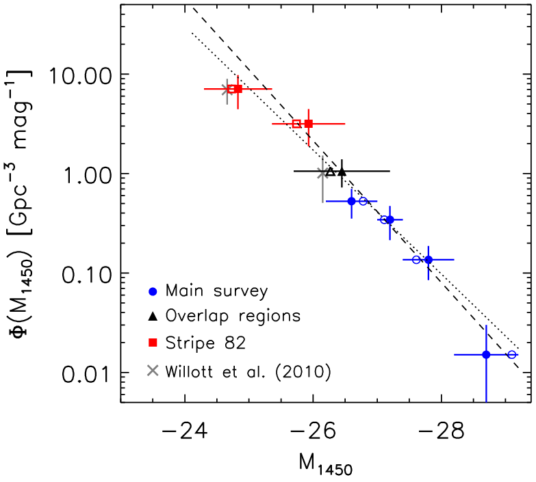
The binned QLF from our SDSS sample in Jiang et al. [52], Jiang et al. [53] is well fit by a single power law , or,
| (1) |
with a steep slope around –2.9. Figure 7 shows that the updated binned QLF can also be described as a power law. The best fit (the dotted line in Figure 7) to all SDSS data points results in a slope of . The fit is dependent on the luminosity bin sizes that we chose. In order to remove this dependence, we use a maximum likelihood analysis to find the best fit. The likelihood function [68, e.g.] is written as
| (2) |
where the sum is over all quasars in the sample, and the integral is over the full luminosity and redshift space of the sample. The best fit is , consistent with the above result.
At low redshift, QLFs are commonly characterized using a double power law,
| (3) |
where is the characteristic magnitude, and is the slope at the faint end. Our SDSS data are apparently not deep enough to reach . However, the recent discovery of much fainter high-redshift quasars [114, 61, 62, 71, e.g.] have suggested a flatter faint-end slope, and the faintest data point in our sample may be affected by the turnover. In order to better constrain the bright-end slope , we also fit a single power law to all SDSS density points but the faintest one in Figure 7, i.e., the luminosity range mag. The best fit is . This is slightly steeper than the slopes found above from the fit to all data points, but is consistent with the value reported by Willott et al. [114]. We thus conclude that the bright-end slope of the QLF is around , and we will adopt in the rest of the paper.
IV.5 Double power law fit to the z6 QLF
We now parametrize the double power law QLF (Equation 3) at . In order to constrain the slope , faint-end data points are required. However, only a small number of quasars discovered so far are fainter than mag [114, 61, 62, 71, e.g.]. In our analysis, we include two faint quasars from Willott et al. [114] and Kashikawa et al. [61]. They are represented as the two faintest data points in Figure 8. Their effective area coverage and sample completeness were carefully derived in the above papers, and have been incorporated into our calculation. We do not include an object in Kashikawa et al. [61] with a narrow Ly line. It is likely a Ly-emitter, not a type 1 quasar or AGN.
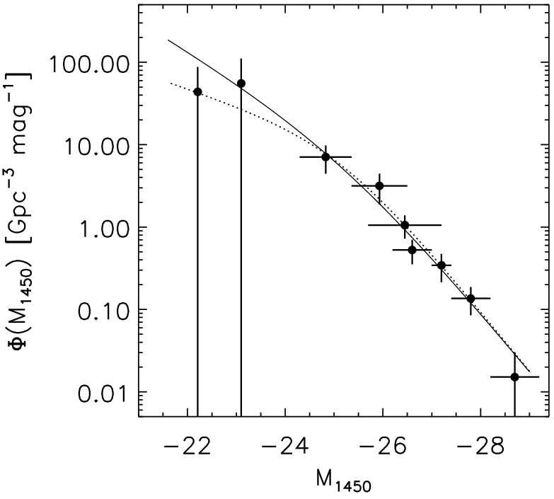
The combined sample is still not sufficient to simultaneously constrain all parameters in Equation 3, thus we choose to fix some of the parameters. We assume that is constant over our redshift range, i.e., . The steep decline of the quasar density at high redshift can be described as [26, 73, e.g.],
| (4) |
Here we assume , derived from the density evolution of luminous quasars from to 6 (see details in Section 5.1). Furthermore, we fix the value of to be , as measured in Section 4.4. We then estimate the faint-end slope and the characteristic magnitude by applying a maximum likelihood analysis to Equation 3. The results are and mag. The resultant from the best fit is 9.93 Gpc-3 mag-1. Thus the best-fit QLF at can be written as,
| (5) |
in units of Gpc-3 mag-1. Note that this is the observed QLF and does not take into account quasar intrinsic properties such as anisotropic emission and dust extinction [22, e.g.].
We perform two-dimensional Kolmogorov-Smirnov (K-S) tests to assess the derived QLF. We generate a large sample () of quasars drawn from the derived QLF (Equation 5), covering the full -redshift space shown in Figure 6. The sample is then convolved with each of the three selection functions to produce three samples of simulated objects. The resultant samples are compared with the three observed quasar samples using the K-S test [84, 31, e.g.]. The probability found in each of the three cases is greater than 0.2, which means that the hypothesis that two data sets are not significantly different is certainly correct. This indicates that the maximum likelihood analysis that we did above is reasonable.
The two free parameters and are poorly constrained as Figure 9 shows; the uncertainties are due to the small number (2) of quasars at the faint end and the degeneracy between and . The real uncertainties are likely to be larger; by fixing and we have not accounted for the uncertainties in those parameters. At low redshift (), the QLF has a very steep bright-end slope and a much flatter faint-end slope [88, 18, 90, e.g.]. The bright-end slope at is found to be quite steep () as well [73, 119, e.g.]. The steep bright-end slope at does not evolve much from those at relatively lower redshifts. On the other hand, the faint-end slope of the optical QLF at has not been well constrained [40, 46, 47, 33, e.g.]. Previous studies of the QLF at usually assumed a fixed slope as found for low-redshift quasars. For example, Willott et al. [114] fixed and found . Their QLF is consistent with ours at the bright end (Figure 8). Our results suggest that the faint-end slope at may be marginally steeper than –1.5 based on the faintest data points shown in Figure 8, as already pointed out by Kashikawa et al. [61] and Matsuoka et al. [71]. However, the large uncertainties on and will not be reduced before a sizable faint quasar sample is obtained.

V Discussion
V.1 Density Evolution of Luminous Quasars at High Redshift
In Section 4.5, we described the quasar density evolution using Equation 4, where . Here we explore in detail the density evolution of luminous quasars at . We work with the integral of the luminosity function from some fiducial lower luminosity to infinity,
| (6) |
In Figure 10, the blue circles show the results at for mag, together with the results at and 5 from McGreer et al. [73]. The slopes of the lines give from to 5, and from to 6. Fan et al. [26] found for quasars brighter than mag at . This value () has been frequently used in more recent papers [114, 73, e.g.]. McGreer et al. [73] noticed that the evolution from to is stronger for quasars brighter than mag, with . We update the density at and find for the same redshift range, which is the same as the value given by McGreer et al. [73].

Alternatively, we add the density evolution to Equation 1, and use the maximum likelihood analysis to find the best fit to a single power law. The result is , consistent with the above result. The large uncertainty is due to the limited sample size, short redshift baseline, and degeneracy between and . Therefore, we chose to use shown in Figure 10. The underlying assumption is that the density evolution at is similar to that at .
Figure 10 shows that the spatial density of luminous quasars from to 6 drops faster than that from to 5 [73, see also]. This trend seems to continue towards higher redshift. So far the QLF at has not been well explored. We estimate the spatial density of luminous quasars at as follows. The UKIDSS team reported a quasar with mag [80], and a quasar with mag [102]. The average effective area is roughly 3370 deg2 for the two quasars (private communication with D.J. Mortlock and S.J. Warren). In order to include the quasar, we integrate Equation 6 down to mag (instead of mag), which is roughly the limit of their quasar selection. Since the selection function for the two quasars has not been calculated, we assume that their selection probability is 1, which would slightly underestimate the density. Given the large statistical uncertainty, the assumption is reasonable for the luminosity regime considered here (brighter than mag). The results are shown in Figure 10. The slope derived for the density evolution between and 7 is .
In addition, we estimate the density evolution of less luminous quasars from to , using three quasars with from the VISTA VIKING survey [101]. The cumulative density is integrated down to mag, which is roughly their quasar survey limit. As shown in Figure 10, the slope is . The above estimate on the density evolution at is rough, based on two very small samples. Nevertheless, the trends seen in Figure 10 suggest a rapid density decline of luminous quasars from towards higher redshifts.
V.2 Quasar Contribution to Reionization
We estimate the quasar contribution to the ionizing background at . We first calculate the number of ionizing photons provided by quasars based on the QLF derived in Section 4. We assume a broken power-law quasar SED as follows [59],
| (7) |
The spectral index may vary with quasar luminosity and background ionization rate [117, e.g.], but we do not consider these complications here. We integrate the SED over an energy range of 1–4 ryd (photons above 4 ryd are consumed by He ii), and integrate the QLF over a luminosity range from to –18 mag. In Figure 11, the blue contours show the computed number of ionizing photons in units of Mpc-3 s-1 as a function of and .
The number of ionizing photons is related to the minimum luminosity that we use in the integral. We use –18 mag in the above calculation, a value which is often used in the literature [69, 39, 61, e.g.]. Giallongo et al. [39] found a sample of very faint AGN candidates with mag at , and estimated that the faint-end slope of the AGN luminosity function was roughly –1.81, consistent with our result of –1.9 at . Their faint AGN sample also suggests that we can integrate the QLF down to at least mag. If we integrate the QLF from to –16 mag, the number of ionizing photons increases by 17% for the best fits shown in Equation 5. AGN luminosities can be even lower [44, 43, e.g.]. In the above calculation, we have assumed that the escape fraction of ionizing photons is 1. In low-luminosity AGN, however, the escape fraction can be much lower [76, e.g.]. We did not take this into account for the luminosity range that we adopted ( mag).

The total photon emissivity per unit comoving volume required to ionize the universe is taken from Madau et al. [69], i.e., where is the clumping factor of the IGM, and we have assumed that the baryon density . The clumping factor is critical as it is closely related to the H recombination rate. Simulations have suggested [75, 32, 94, e.g.]. In Figure 11, we show the required photon emissivity (red dashed curves) for three representative values, 1.5, 3, and 5. The figure clearly shows the following.
- 1.
The significance of the quasar contribution to the ionizing background strongly depends on , , and .
- 2.
If , the quasar/AGN population cannot provide enough photons to ionize the IGM (at % confidence). We can also rule out at % confidence that the quasar/AGN population can provide 50% of the required photons.
- 3.
If , the quasar/AGN population can provide enough photons only if the faint-end slope is significantly steeper than –2 and/or the characteristic luminosity is very low.
The conclusion that a faint-end slope at the steep end of current observations is required for quasars to generate sufficient photons to ionize the Universe at is generally robust; however, it is worth restating some of the key assumptions that went into the above calculations. We assumed a constant , and fixed and when we calculated the QLF. These choices will underestimate the uncertainties in and . We chose a magnitude limit of mag, which extends well below current observations. We further assumed an escape fraction of unity for ionizing photons, independent of quasar luminosity. Finally, we assumed a relatively small range of clumping factors based on current theoretical models.
It is generally thought that low-luminosity star-forming galaxies may provide enough ionizing photons for cosmic reionization, while the contribution from quasars/AGN is probably negligible due to their low spatial density. Figure 11 shows that we cannot yet fully rule out the probability that UV light from AGN is responsible for ionizing the universe [39, 70, 77, see also e.g.,]; however, current observations do not favor this scenario. Future deep surveys of quasars at will provide a definitive answer.
VI Summary
In this paper, we have presented the discovery of nine quasars at identified in the SDSS, including seven quasars in the SDSS main survey, one quasar in the overlap regions, and one quasar in Stripe 82. One of the quasars in the main survey, J1148+0702 at , is the second highest-redshift quasar found in the SDSS. This completes our survey of quasars in the SDSS footprint. We summarized our final sample of 52 SDSS quasars at . In total, we have found (1) 29 quasars in 11,240 deg2 of the SDSS main survey; (2) 17 quasars in 4223 deg2 of the overlap regions (7 of which are in common with the main survey sample); (3) 13 quasars in 277 deg2 of Stripe 82. The main survey quasars are the most luminous quasars, with mag. The overlap region quasars are roughly 0.5 mag fainter, and the Stripe 82 quasars are 2 mag fainter. The quasars span a wide luminosity range of mag, and comprise a well-defined quasar sample at .
Based on the combination of our new quasar sample and two much fainter quasars in the literature, we obtained parameters for a double power-law fit to the QLF at using a maximum likelihood analysis. The bright end of the QLF is well constrained, and the slope is steep with . The best-fitting results for the faint-end slope and the characteristic magnitude are and mag, and the two quantities are strongly correlated. The large uncertainties are due to the small number of quasars at the faint end. We calculated the cumulative density of luminous quasars ( mag, mag, and mag) at and 7, and compared them with those at and 5. We found that the cumulative density at declines rapidly towards higher redshift. We estimated the quasar contribution to the ionizing background at using the derived QLF. Assuming an IGM clumping factor , the quasar population cannot provide enough photons to ionize the IGM (at % confidence). We found that quasars can provide enough photons only if the faint-end slope is steeper than –2 and/or if the characteristic luminosity is very low. A large sample of very faint quasars ( mag) is needed to provide a better constraint on the quasar contribution to cosmic reionization.
Many quasars in our sample have been extensively studied in multiple wavelength bands from X-ray to radio. More observations are being carried out and being planned. For example, we are carrying out deep near-IR spectroscopy of quasars at using Gemini GNIRS. When this program completes, we will have near-IR (or rest-frame UV) spectra for all the SDSS quasars. These spectra will allow us to measure various quasar properties, such as spectral index and emission line properties, metallicity in the broad-line region, central black-hole mass, and so on. The well-defined sample will enable us to derive the black-hole mass function at , and further constrain the birth and growth of the earliest massive black holes. We are also gathering mm/submm observations using ALMA, IRAM, and JCMT for our SDSS sample [107, 108, e.g.]. These observations provide rich information on dust emission, star formation, and dynamical properties of quasar host galaxies, in the context of galaxy – black hole co-evolution at the early epoch. Therefore, this unique SDSS sample will have a legacy value for exploring the distant universe in the future.
Meanwhile, ongoing and future large-area surveys are finding high-redshift quasars in large numbers. For example, Pan-STARRS1 has found more than 100 quasars [6], and will improve the constraint on the bright-end QLF at . Note that the measurement of the quasar density at the brightest end ( mag) will not be improved by more than a factor of two, since the SDSS already covers one fourth of the whole sky. With near-IR imaging, the VISTA VIKING survey is able to find higher redshift quasars. It has found 3 quasars at , and is expecting to find nearly 20 quasars at in the near future [101]. DES, with imaging data slightly deeper than Stripe 82 over deg2, has found its first quasar, and has claimed that it would find 50–100 quasars at , including 3–10 quasars at [87]. The Subaru SHELLQ survey is producing a large number of very faint quasars using deep Hyper Suprime-Cam imaging data [71]. These quasars will be used to constrain the faint end of the QLF at . The future LSST survey [49] will have an unprecedented power for searches of high-redshift quasars. It will eventually find thousands of quasars (assuming that there will be enough resources for follow-up identification), and fully constrain the QLF. The above surveys are providing a golden opportunity for studying high-redshift quasars and the distant universe.
Appendix A The optical spectra of the 52 SDSS quasars at
Figure 12 shows the optical spectra of the 52 SDSS quasars at , ordered by redshift. The numbers of the quasars correspond to the numbers in Column 1 of Table 2. Most of the spectra were taken from the quasar discovery papers listed in Column 13 of Table 2. All spectra have been binned to 10 Å per pixel. The figure can be downloaded from http://kiaa.pku.edu.cn/~jiang/SDSS52spectra.eps, or http://kiaa.pku.edu.cn/~jiang/SDSS52spectra2.eps.

References
- [1] Adelman-McCarthy, J. K., Agüeros, M. A., Allam, S. S., et al. 2007, ApJS, 172, 634
- [2] Aihara, H., Allende Prieto, C., An, D., et al. 2011, ApJS, 193, 29
- [3] Annis, J., Soares-Santos, M., Strauss, M. A., et al. 2014, ApJ, 794, 120
- [4] Bañados, E., Venemans, B. P., Morganson, E., et al. 2014, AJ, 148, 14
- [5] Bañados, E., Decarli, R., Walter, F., et al. 2015, ApJ, 805, L8
- [6] Bañados, E., et al. 2016, ApJS, in press (arXiv:1608.03279)
- [7] Barnett, R., Warren, S. J., Banerji, M., et al. 2015, A&A, 575, A31
- [8] Becker, R. H., Fan, X., White, R. L., et al. 2001, AJ, 122, 2850
- [9] Becker, G. D., Sargent, W. L. W., Rauch, M., & Calverley, A. P. 2011, ApJ, 735, 93
- [10] Becker, G. D., Bolton, J. S., Madau, P., et al. 2015, MNRAS, 447, 3402
- [11] Blain, A. W., Assef, R., Stern, D., et al. 2013, ApJ, 778, 113
- [12] Bolton, J. S., Haehnelt, M. G., Warren, S. J., et al. 2011, MNRAS, 416, L70
- [13] Brown, W. R., McLeod, B. A., Geary, J. C., & Bowsher, E. C. 2008, Proc. SPIE, 7014, 70142P
- [14] Calura, F., Gilli, R., Vignali, C., et al. 2014, MNRAS, 438, 2765
- [15] Carilli, C. L., Wang, R., Fan, X., et al. 2010, ApJ, 714, 834
- [16] Carilli, C. L., & Walter, F. 2013, ARA&A, 51, 105
- [17] Carnall, A. C., Shanks, T., Chehade, B., et al. 2015, MNRAS, 451, L16
- [18] Croom, S. M., Richards, G. T., Shanks, T., et al. 2009, MNRAS, 399, 1755
- [19] Cool, R. J., Kochanek, C. S., Eisenstein, D. J., et al. 2006, AJ, 132, 823
- [20] De Rosa, G., Decarli, R., Walter, F., et al. 2011, ApJ, 739, 56
- [21] De Rosa, G., Venemans, B. P., Decarli, R., et al. 2014, ApJ, 790, 145
- [22] DiPompeo, M. A., Myers, A. D., Brotherton, M. S., Runnoe, J. C., & Green, R. F. 2014, ApJ, 787, 73
- [23] Fan, X. 1999, AJ, 117, 2528
- [24] Fan, X., White, R. L., Davis, M., et al. 2000, AJ, 120, 1167
- [25] Fan, X., Narayanan, V. K., Lupton, R. H., et al. 2001, AJ, 122, 2833
- [26] Fan, X., Strauss, M. A., Schneider, D. P., et al. 2001, AJ, 121, 54
- [27] Fan, X., Strauss, M. A., Schneider, D. P., et al. 2003, AJ, 125, 1649
- [28] Fan, X., Hennawi, J. F., Richards, G. T., et al. 2004, AJ, 128, 515
- [29] Fan, X., Strauss, M. A., Richards, G. T., et al. 2006, AJ, 131, 1203
- [30] Fan, X., Strauss, M. A., Becker, R. H., et al. 2006, AJ, 132, 117
- [31] Fasano, G., & Franceschini, A. 1987, MNRAS, 225, 155
- [32] Finlator, K., Oh, S. P., Özel, F., & Davé, R. 2012, MNRAS, 427, 2464
- [33] Fiore, F., Puccetti, S., Grazian, A., et al. 2012, A&A, 537, A16
- [34] Fliri, J., & Trujillo, I. 2016, MNRAS, 456, 1359
- [35] Gallerani, S., Maiolino, R., Juarez, Y., et al. 2010, A&A, 523, A85
- [36] Górski, K. M., Hivon, E., Banday, A. J., et al. 2005, ApJ, 622, 759
- [37] Goto, T. 2006, MNRAS, 371, 769
- [38] Fukugita, M., Ichikawa, T., Gunn, J. E., et al. 1996, AJ, 111, 1748
- [39] Giallongo, E., Grazian, A., Fiore, F., et al. 2015, A&A, 578, A83
- [40] Glikman, E., Djorgovski, S. G., Stern, D., et al. 2011, ApJ, 728, L26
- [41] Gunn, J. E., Carr, M., Rockosi, C., et al. 1998, AJ, 116, 3040
- [42] Gunn, J. E., Siegmund, W. A., Mannery, E. J., et al. 2006, AJ, 131, 2332
- [43] Hao, L., Strauss, M. A., Fan, X., et al. 2005, AJ, 129, 1795
- [44] Ho, L. C., Filippenko, A. V., & Sargent, W. L. W. 1997, ApJS, 112, 315
- [45] Hogg, D. W., Finkbeiner, D. P., Schlegel, D. J., & Gunn, J. E. 2001, AJ, 122, 2129
- [46] Ikeda, H., Nagao, T., Matsuoka, K., et al. 2011, ApJ, 728, L25
- [47] Ikeda, H., Nagao, T., Matsuoka, K., et al. 2012, ApJ, 756, 160
- [48] Ivezić, Ž., Lupton, R. H., Schlegel, D., et al. 2004, Astronomische Nachrichten, 325, 583
- [49] Ivezic, Z., Axelrod, T., Brandt, W. N., et al. 2008, Serbian Astronomical Journal, 176, 1
- [50] Jiang, L., Fan, X., Hines, D. C., et al. 2006, AJ, 132, 2127
- [51] Jiang, L., Fan, X., Vestergaard, M., et al. 2007, AJ, 134, 1150
- [52] Jiang, L., Fan, X., Annis, J., et al. 2008, AJ, 135, 1057
- [53] Jiang, L., Fan, X., Bian, F., et al. 2009, AJ, 138, 305
- [54] Jiang, L., Fan, X., Brandt, W. N., et al. 2010, Nature, 464, 380
- [55] Jiang, L., Fan, X., Bian, F., et al. 2014, ApJS, 213, 12
- [56] Jiang, L., McGreer, I. D., Fan, X., et al. 2015, AJ, 149, 188
- [57] Juarez, Y., Maiolino, R., Mujica, R., et al. 2009, A&A, 494, L25
- [58] Jun, H. D., Im, M., Lee, H. M., et al. 2015, ApJ, 806, 109
- [59] Lusso, E., Worseck, G., Hennawi, J. F., et al. 2015, MNRAS, 449, 4204
- [60] Kaiser, N., Burgett, W., Chambers, K., et al. 2010, Proc. SPIE, 7733, 77330E
- [61] Kashikawa, N., Ishizaki, Y., Willott, C. J., et al. 2015, ApJ, 798, 28
- [62] Kim, Y., Im, M., Jeon, Y., et al. 2015, ApJ, 813, L35
- [63] Kurk, J. D., Walter, F., Fan, X., et al. 2007, ApJ, 669, 32
- [64] Kurk, J. D., Walter, F., Fan, X., et al. 2009, ApJ, 702, 833
- [65] Leipski, C., Meisenheimer, K., Walter, F., et al. 2014, ApJ, 785, 154
- [66] Lupton, R., Gunn, J. E., Ivezić, Z., Knapp, G. R., & Kent, S. 2001, Astronomical Data Analysis Software and Systems X, 238, 269
- [67] Lyu, J., Rieke, G. H., & Alberts, S. 2016, ApJ, 816, 85
- [68] Marshall, H. L., Avni, Y., Tananbaum, H., & Zamorani, G. 1983, ApJ, 269, 35
- [69] Madau, P., Haardt, F., & Rees, M. J. 1999, ApJ, 514, 648
- [70] Madau, P., & Haardt, F. 2015, ApJ, 813, L8
- [71] Matsuoka, Y., Onoue, M., Kashikawa, N., et al. 2016, ApJ, 828, 26
- [72] McGreer, I. D., Becker, R. H., Helfand, D. J., & White, R. L. 2006, ApJ, 652, 157
- [73] McGreer, I. D., Jiang, L., Fan, X., et al. 2013, ApJ, 768, 105
- [74] McGreer, I. D., Mesinger, A., & D’Odorico, V. 2015, MNRAS, 447, 499
- [75] McQuinn, M., Oh, S. P., & Faucher-Giguère, C.-A. 2011, ApJ, 743, 82
- [76] Micheva, G., Iwata, I., & Inoue, A. K. 2016, MNRAS, in press (arXiv:1604.00102)
- [77] Mitra, S., Choudhury, T. R., & Ferrara, A. 2016, MNRAS, summited (arXiv:1606.02719)
- [78] Morganson, E., De Rosa, G., Decarli, R., et al. 2012, AJ, 143, 142
- [79] Mortlock, D. J., Patel, M., Warren, S. J., et al. 2009, A&A, 505, 97
- [80] Mortlock, D. J., Warren, S. J., Venemans, B. P., et al. 2011, Nature, 474, 616
- [81] Mortlock, D. J. 2015, arXiv:1511.01107
- [82] Omont, A., Willott, C. J., Beelen, A., et al. 2013, A&A, 552, A43
- [83] Padmanabhan, N., Schlegel, D. J., Finkbeiner, D. P., et al. 2008, ApJ, 674, 1217
- [84] Peacock, J. A. 1983, MNRAS, 202, 615
- [85] Pier, J. R., Munn, J. A., Hindsley, R. B., et al. 2003, AJ, 125, 1559
- [86] Plotkin, R. M., Shemmer, O., Trakhtenbrot, B., et al. 2015, ApJ, 805, 123
- [87] Reed, S. L., McMahon, R. G., Banerji, M., et al. 2015, MNRAS, 454, 3952
- [88] Richards, G. T., Strauss, M. A., Fan, X., et al. 2006, AJ, 131, 2766
- [89] Ross, N. P., Myers, A. D., Sheldon, E. S., et al. 2012, ApJS, 199, 3
- [90] Ross, N. P., McGreer, I. D., White, M., et al. 2013, ApJ, 773, 14
- [91] Schmidt, G. D., Weymann, R. J., & Foltz, C. B. 1989, PASP, 101, 713
- [92] Shen, Y., Strauss, M. A., Oguri, M., et al. 2007, AJ, 133, 2222
- [93] Shen, Y., & Liu, X. 2012, ApJ, 753, 125
- [94] Shull, J. M., Harness, A., Trenti, M., & Smith, B. D. 2012, ApJ, 747, 100
- [95] Simcoe, R. A., Cooksey, K. L., Matejek, M., et al. 2011, ApJ, 743, 21
- [96] Skrutskie, M. F., Cutri, R. M., Stiening, R., et al. 2006, AJ, 131, 1163
- [97] Smith, J. A., Tucker, D. L., Kent, S., et al. 2002, AJ, 123, 2121
- [98] Strauss, M. A., Fan, X., Gunn, J. E., et al. 1999, ApJ, 522, L61
- [99] Tucker, D. L., Kent, S., Richmond, M. W., et al. 2006, Astronomische Nachrichten, 327, 821
- [100] Venemans, B. P., McMahon, R. G., Warren, S. J., et al. 2007, MNRAS, 376, L76
- [101] Venemans, B. P., Findlay, J. R., Sutherland, W. J., et al. 2013, ApJ, 779, 24
- [102] Venemans, B. P., Bañados, E., Decarli, R., et al. 2015, ApJ, 801, L11
- [103] Walter, F., Riechers, D., Cox, P., et al. 2009, Nature, 457, 699 et al. 2013, ApJ, 773, 44
- [104] Wang, F., Wu, X.-B., Fan, X., et al. 2016, ApJ, 819, 24
- [105] Wang, R., Carilli, C. L., Wagg, J., et al. 2008, ApJ, 687, 848-858
- [106] Wang, R., Wagg, J., Carilli, C. L., et al. 2011, AJ, 142, 101
- [107] Wang, R., Wagg, J., Carilli, C. L., et al. 2013, ApJ, 773, 44
- [108] Wang, R., Wu, X.-B., Neri, R., et al. 2016, ApJ, in press (arXiv:1606.09634)
- [109] Warren, S. J., Hambly, N. C., Dye, S., et al. 2007, MNRAS, 375, 213
- [110] White, R. L., Becker, R. H., Fan, X., & Strauss, M. A. 2003, AJ, 126, 1
- [111] Willott, C. J., Delorme, P., Omont, A., et al. 2007, AJ, 134, 2435
- [112] Willott, C. J., Delorme, P., Reylé, C., et al. 2009, AJ, 137, 3541
- [113] Willott, C. J., Albert, L., Arzoumanian, D., et al. 2010a, AJ, 140, 546
- [114] Willott, C. J., Delorme, P., Reylé, C., et al. 2010b, AJ, 139, 906
- [115] Wright, E. L., Eisenhardt, P. R. M., Mainzer, A. K., et al. 2010, AJ, 140, 1868-1881
- [116] Wu, X.-B., Wang, F., Fan, X., et al. 2015, Nature, 518, 512
- [117] Wyithe, J. S. B., & Bolton, J. S. 2011, MNRAS, 412, 1926
- [118] Yan, L., Donoso, E., Tsai, C.-W., et al. 2013, AJ, 145, 55
- [119] Yang, J., Wang, F., Wu, X., et al. 2016, ApJ, in press (arXiv:1607.04415)
- [120] York, D. G., Adelman, J., Anderson, J. E., Jr., et al. 2000, AJ, 120, 1579
- [121] Zeimann, G. R., White, R. L., Becker, R. H., et al. 2011, ApJ, 736, 57