Sensitivity of Complex Networks
Abstract.
The sensitivity (i.e. dynamic response) of complex networked systems has not been well understood, making difficult to predict whether new macroscopic dynamic behavior will emerge even if we know exactly how individual nodes behave and how they are coupled. Here we build a framework to quantify the sensitivity of complex networked system of coupled dynamic units. We characterize necessary and sufficient conditions for the emergence of new macroscopic dynamic behavior in the thermodynamic limit. We prove that these conditions are satisfied only for architectures with power-law degree distributions. Surprisingly, we find that highly connected nodes (i.e. hubs) only dominate the sensitivity of the network up to certain critical frequency.
1. Introduction
Understanding how macroscopic dynamic behavior can emerge from a networked system of many agents (or units) is a fundamental question in physics [1, 2]. Addressing this question also has implications in biology [3], engineering [4] and cognitive science [5]. Complex behavior can emerge purely from nonlinear dynamics —through bifurcations [6], catastrophes [7], strange attractors [8] and so on— but may also emerge due to the aggregation of a large number of agents with simple nodal dynamics in the so-called thermodynamic limit. A famous example is Boltzmann’s -theorem, where agents with time-reversible nodal dynamics give rise to macroscopic irreversible behavior [9]. However, it remains unclear how and when the properties of this aggregation —given by the network describing which agent interacts with whom— will lead to the emergence of new macroscopic dynamic behavior.
Here we introduce a framework to study the sensitivity (i.e. dynamic response) of networked systems and investigate the conditions for the emergence of new macroscopic behavior. We first analyze how the degree of a node in the network shape its contribution to the dynamic response of the system. We find that in systems with high-order nodal dynamics, the hubs (i.e., high-degree nodes) not always dominate the dynamic response of the system. In other words, nodes important from a network perspective are not as important from a dynamic perspective. Indeed, with second-order oscillatory dynamics, we find there is a transition point close to the resonant frequency of the dynamics where hubs lose their dominant role. Then we study how the interconnection topology of a system (i.e., the network topology) shapes its macroscopic or collective behavior, finding that the degree distribution of the network is sufficient to constraint the emergence of new behavior. We rigorously prove that new behavior emerges if and only if no eigenvector of the interconnection network aligns with the vector . In other words, new behavior emerges if and only if the system cannot fully synchronize. In particular, we show that new behavior cannot emerge in the thermodynamic limit using interconnection networks with Erdos-Renyi architecture, in the sense that their dynamic behavior can be reproduced by the dynamics of a single node. In contrast, we prove that new behavior emerges with degree distributions with heavy tails, e.g., power-law degree distributions in scale-free networks.
2. Model
In order to focus on the role of the aggregation, we assume that each node (agent) has a simple linear dynamics. Under this assumption, a broad class of dynamic systems describing interacting agents in an undirected network can be described by
| (1) |
where with the activity of node . The network underlying the system is encoded by the symmetric interaction matrix , representing the direct interactions between the agents: if nodes and directly interact (i.e., contains a link between nodes and ) and otherwise. The nonzero edge-weights are given by where represents the interaction strength between agents and . We assume the ’s follow a fixed distribution that we choose over the interval without loss of generality. The mean degree of the network acts as a scaling factor that is necessary to obtain a bounded mathematical object when we take the thermodynamic limit . Dynamics enter (1) through , where is a linear causal operator acting on the trajectory of each node and is the identity matrix of dimension . For example, if is the derivative operator then (1) is the first-order system usually found in diffusion or consensus [10]. In the case then (1) becomes , which represents coupled oscillators with damping and natural frequency often used for modeling the power-grid [11].
It is convenient to rewrite system (1) in the Laplace domain
| (2) |
where is the Laplace transform of , is the Laplace variable, and is a vector of initial conditions of the system11 1 Recall that in Laplace domain, the derivative operator is given by multiplication by . Therefore, when then and . But if then and . Then, equation (2) can be rewritten as
where maps initial conditions to trajectories, and thus is known as the transfer or sensitivity function of the system [12].
3. Results
To obtain the macroscopic behavior of the system, assume that all agents start from the same initial condition , , , where . Consequently, and the dynamic behavior of each agent in the system is , where
is an -dimensional vector containing the node sensitivity. This vector characterizes the dynamic response of each agent of the system. Similarly, the average or macroscopic behavior of the system is given by , where
is the mean sensitivity or mean transfer function of the system, characterizing its average dynamic behavior. With this notation the dynamic behavior of the isolated agents (i.e. ) is and the dynamic behavior of the system in the thermodynamic limit is .

With the above framework, new behavior emerges when cannot be approximated by . One method to quantify the difference between and is comparing their frequency responses or Fourier transforms. The frequency response is obtained from the Laplace transform by substituting , and letting the frequency vary from to . Then, is near if the complex number is near for . We can graphically read this more conveniently using Bode plots of magnitude and phase, Fig. 1.
3.1. Node-level sensitivity
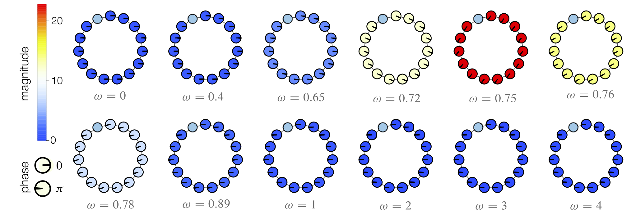
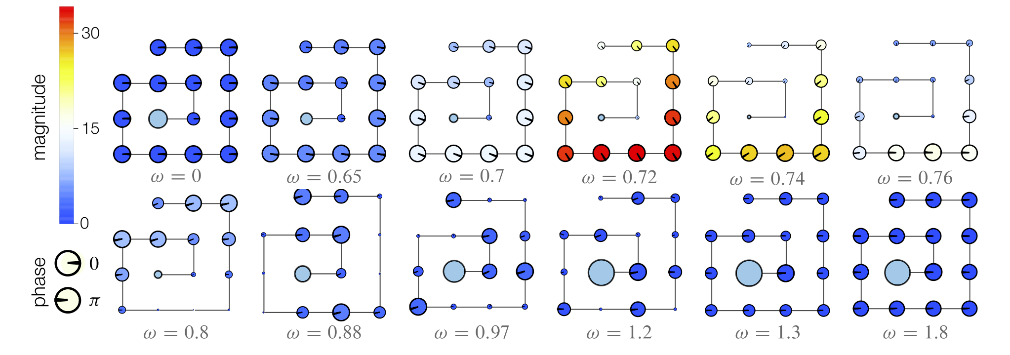
The node level sensitivity characterizes the nodes that are important from a dynamical viewpoint, assuming all agents start from the same initial condition. In this case, the dynamic response of node at frequency is the -th element of the vector . Naturally, the elements of with larger magnitude contribute more to the average behavior of the system at frequency . As shown in Fig. 2, for second-order dynamics, the hubs dot not always have the response with largest magnitude. For example, in the star network, the central hub has a larger magnitude than the leaf nodes at low frequencies, but smaller magnitude at high frequencies. Indeed, we observe that the leaf nodes are always synchronized (i.e., have equal phase), but they are not always synchronized with the hub. Since the response of each node is a weighted sum of its nearest neighbors (note that this is a sum of complex numbers), the contribution of the hub is maximal at because the leaves and hub synchronize. In contrast, at , the hub and the leaves are anti-synchronized (i.e., have opposite phases) and now the leaves inhibit the response of the hub.
We found a similar phenomenon in larger networks with second order dynamics —using networks either randomly generated or real ones such as a power grid— irrespectively of the distribution of the edge-weights, Fig.3. Nodes in a power grid correspond to generators, and a standard model for their dynamics is the so-called “swing dynamics”, which is linear and of second order [11]. When the dynamics are of first order, this phenomenon disappears. Real systems always contain high-order dynamics —in principle, any system can be modeled with arbitrary high precision by a linear model with sufficiently high order— and hence this result shows that the topological properties of the interconnection network do not determine completely the nodes that dominate the response of the system at all frequencies. In other words, if we are interested in understanding the low-frequency dynamics of a networked system it is enough to focus on the most connected agents such as the hubs. However, in order to understand the high-frequency dynamics of a networked system, we must consider the agents which are in the “periphery” of the network. This counterintuitive effect of weakly connected nodes illustrates the rich interplay between networks and dynamics in complex systems.



3.2. Network-level sensitivity
The network-level sensitivity characterizing the macroscopic dynamic behavior of the system depends on the network encoded in the interaction matrix . In principle, one expects that networks with different edge-weights or interconnection topologies (e.g., Erdos-Renyi or scale-free topologies) produce different mean sensitivities (Fig.2). In what follows we show this is not the case in the thermodynamic limit , and that there are two “sensitivity classes” —in the first, the mean behavior of the system equals the behavior of the isolated nodes, and in the second new behavior emerges— that depend on the heterogeneity of connections of the network only.
First rewrite in terms of the eigenvalues , and eigenvectors of , yielding
| (3) |
where . This equation shows that the average response of the system is a weighted sum of the functions . Hence new behavior emerges if and only if no eigenvector aligns with the vector . Since is symmetric, the eigenvectors can be chosen real, orthogonal and with unit norm, so they satisfy
| (4) |
where .
From equations (3) and (4), we conclude that can be approximated by if and only if one term in the sum (4) dominates as . We can prove that when the interconnection network is an Erdös-Renyi (ER) network then as (Theorem 1 in SI). Therefore, the weight associated to the first eigenvalue is dominant
where is the probability of connection in the ER random network model. This implies that the contribution of the residue vanishes in the thermodynamic limit, and that . Consequently, assuming the system is stable, these two results imply that
showing that new dynamic behavior cannot emerge in ER networks. For example, considering to be the oscillator dynamics then we have that
is again an oscillator with parameters , and . Numerical experiments show that several other interconnection topologies such as lattices, small-world or random geometric networks also belong to this first class in which new macroscopic behavior do not emerge (Fig. 5). Note also that, due to the law of large numbers, the thermodynamic limit of a network without structure (i.e., is the complete graph on nodes) also belongs this first class.
The situation is drastically different in networks with heavy-tailed degree distribution . In Theorem 2 of SI, we proved that if the contribution due to the first eigenvalue satisfies
where . This implies that and the dynamic behavior in thermodynamic limit is opposite to ER networks: the response due to the first term vanishes as and the residue dominates. Furthermore, the weight of all other eigenvectors remain approximately the same. This fundamental distinction of networks with heavy-tailed degree distribution becomes evident by comparing their frequency responses, Fig. 4. Only in these networks do we observe two peaks in their frequency response that cannot be approximated by the response of an isolated node (which has a single bump corresponding to the resonance peak). Thus, the thermodynamic limit of SF networks belong to a second sensitivity class in which new macroscopic behavior emerges.

4. Outlook and concluding remarks
Large systems can exhibit complex behavior due to their dynamics and/or due to the properties of its interconnection network. By focusing on linear dynamics, we have shown that very coarse properties of the interconnection network such as its degree sequence can determine the macroscopic behavior of the system. We found that homogenous interconnections (as cycles) tend to produce similar dynamic response in all nodes in the network. But heterogeneous interconnections (like stars or even paths) cause that each node contributes differently to the response and the system, with magnitude and phase depending on the specific frequency that is excited. We identified the mechanism through which the interconnection network favors the emergence of new behavior in the thermodynamic limit. New behavior emerges when the eigenvectors of the interconnection network do not align with the vector , which represents consensus. Furthermore, we showed there are two sensitivity classes, one in which new behavior does not emerge —containing unstructured, ER and several other topologies— and the other in which new behavior emerges —containing SF networks. A similar analysis for the case of directed graphs remains open, mainly due to the fact that the spectral theory of random directed graphs is not as developed as in the case of undirected graphs. Also, a better understanding of how nonlinearities and heterogeneities in the node dynamics may affect wether the system belongs to the first or second sensitivity class can provide further insights into the role of the interconnection network in the emergence of macroscopic behavior.
References
- [1] P. W. Anderson et al., “More is different,” Science, vol. 177, no. 4047, pp. 393–396, 1972.
- [2] M. Gu, C. Weedbrook, Á. Perales, and M. A. Nielsen, “More really is different,” Physica D: Nonlinear Phenomena, vol. 238, no. 9, pp. 835–839, 2009.
- [3] L. A. Amaral, A. Díaz-Guilera, A. A. Moreira, A. L. Goldberger, and L. A. Lipsitz, “Emergence of complex dynamics in a simple model of signaling networks,” Proceedings of the National Academy of Sciences of the United States of America, vol. 101, no. 44, pp. 15551–15555, 2004.
- [4] M. Niazi, A. Hussain, et al., “Sensing emergence in complex systems,” Sensors Journal, IEEE, vol. 11, no. 10, pp. 2479–2480, 2011.
- [5] E. Thompson and F. J. Varela, “Radical embodiment: neural dynamics and consciousness,” Trends in cognitive sciences, vol. 5, no. 10, pp. 418–425, 2001.
- [6] C. Sparrow, The Lorenz equations: bifurcations, chaos, and strange attractors, vol. 41. Springer Science & Business Media, 2012.
- [7] V. I. Arnol’d, Catastrophe theory. Springer Science & Business Media, 1992.
- [8] S. H. Strogatz, Nonlinear dynamics and chaos: with applications to physics, biology, chemistry, and engineering. Westview press, 2014.
- [9] C. Villani, H-Theorem and beyond: Boltzmann’s entropy in today’s mathematics. na, 2008.
- [10] J.-C. Delvenne, R. Lambiotte, and L. E. Rocha, “Diffusion on networked systems is a question of time or structure,” Nature communications, vol. 6, 2015.
- [11] P. Kundur, N. J. Balu, and M. G. Lauby, Power system stability and control, vol. 7. McGraw-hill New York, 1994.
- [12] K. J. Aström and R. M. Murray, Feedback systems: an introduction for scientists and engineers. Princeton university press, 2010.