On Finding Small Sets that Influence
Large Networks Thanks: A preliminary version of this paper was presented at the 1st International Workshop on Dynamics in Networks (DyNo 2015) in conjunction with the 2016 IEEE/ACM International Conference ASONAM, Paris, France, August 25-28, 2015. [21]

Gennaro Cordasco Affiliation: Dept. of Psychology Affiliation: Second University of Naples, Italy Luisa Gargano Affiliation: Dept. of Computer Science Affiliation: University of Salerno, Italy Adele Anna Rescigno Affiliation: Dept. of Computer Science Affiliation: University of Salerno, Italy

Abstract

We consider the problem of selecting a minimum size subset of nodes in a network, that allows to activate all the nodes of the network. We present a fast and simple algorithm that, in real-life networks, produces solutions that outperform the ones obtained by using the best algorithms in the literature. We also investigate the theoretical performances of our algorithm and give proofs of optimality for some classes of graphs. From an experimental perspective, experiments also show that the performance of the algorithms correlates with the modularity of the analyzed network. Moreover, the more the influence among communities is hard to propagate, the less the performances of the algorithms differ. On the other hand, when the network allows some propagation of influence between different communities, the gap between the solutions returned by the proposed algorithm and by the previous algorithms in the literature increases.

1 Introduction

The study of networked phenomena has experienced a particular surge of interest over the past decade, thanks to the large diffusion of social networks which led to increasing availability of huge amounts of data in terms of static network topology as well as the dynamic of interactions among users [41].
A large part of such studies deals with the analysis of influence spreading in social networks. Social influence is the process by which individuals, interacting with other people, change or adapt their attitude, belief or behavior in order to fit in with a group [13]. Commercial companies, as well as politician, have soon recognized that they can benefit from a social influence process which advertises their product (or belief) from one person to another [4, 32, 40, 38] . This advertising process is well known as viral marketing [33]. A key research question in the area of viral marketing is how to efficiently identify a set of users which are able to widely disseminate a certain information within the network. This matter suggests several optimization problems. Some of them were first articulated in the seminal papers [23, 29, 30], under various influence propagation models. A description of the area can be found in the recent monograph [7].

In this paper we consider the Minimum Target Set problem which, roughly speaking, asks for selecting a minimum size subset of nodes in a network that once active are able to activate all the nodes of the network under the Linear Threshold (LT) influence propagation model. According to the LT model, a user $v$ becomes active when the sum of influences of its neighbors in the networks reaches a certain threshold $t(v)$ [28]. The formal definition of the Minimum Target Set problem is given in Section 2.
Chen [6] studied the Minimum Target Set problem under the LT model and proved a strong inapproximability result that makes unlikely the existence of an algorithm with approximation factor better than $O(2^{\log^{1-\epsilon}n})$ , where $n$ is the number of nodes in the network. Chen’s result stimulated a series of papers that isolated interesting cases in which the problem (and variants thereof) becomes tractable [1, 2, 3, 5, 10, 11, 12, 14, 15, 16, 18, 19, 20, 26, 36, 37, 43].
In the case of general networks, some efficient heuristics for the Minimum Target Set problem have been proposed in the literature [17, 22, 39]. In particular, Shakarian et al. [39] introduced a deprecation based approach where the algorithm iteratively deprecates (i.e., removes from the network) the less influencing nodes. The output set is determined, in this case, by the nodes that remain in the network. Subsequently, the authors of [17] proposed a novel deprecation-like approach which, from the theoretically point of view, always produces optimal solution (i.e, a minimum size subset of nodes that influence the whole network) for trees, cycles and cliques and on real life networks produces solutions that outperform the ones obtained using previous algorithms [22, 39].

1.1 Our Results

In this paper we present an evolution of the heuristics in [17]. It is an extension from undirected to directed networks that allows the additional feature of taking into account the influence that a deprecated node may apply on his outgoing neighbors. This extension allows to strongly improve the quality of the obtained solution. Indeed, in the previous deprecation-based algorithms for the Minimum Target Set problem, once a node was determined as irrelevant, it was immediately pruned from the network and so its potential influence was lost. This novel approach has been first introduced and experimentally evaluated in [21]. Here we present a theoretical analysis of this approach together with a deeper experimental analysis. We will show that although the new heuristic is not always better than the one in [17] (an example of such a rare case is provided in Section 4), the novel approach has the following properties:

$\bullet$

It always produces an optimal solution for several classes of networks;
$\bullet$

it always produces a solution $S$ of bounded cardinality matching the upper bound given in [1] and [17].

From a practical point of view, in real-life networks, experiments show that:

$\bullet$

The proposed algorithm produces solutions that always outperform the ones obtained using the known algorithms which have a comparable running time [17, 39];
$\bullet$

the performance of algorithms for the Minimum Target Set problem correlates with the network modularity, which measures the strength of the network subdivision into communities. If the modularity is high then the influence is hard to propagate among communities; on the other hand, when the network allows the propagation of influence between different communities, the performance of the algorithms increases. This correlation becomes stronger for the algorithm proposed in this paper. Such a result is probably due to the capability of our algorithm to better exploit situations where the community structure of the networks allows some influence propagation between different communities.

2 The Minimum Target Set Problem

We represent a social network by means of a directed graph $G=(V,E)$ where an arc $(u,v)$ represents the capability of $u$ of influencing $v$ .
A threshold function $t:V\to{\mathbb{N}}=\{0,1,2,\ldots\}$ assigns non negative integers to the nodes of $G$ : For each node $v\in V$ , the value $t(v)$ measures the conformity of node $v$ , in the sense that an easy-to-conform element $v$ of the network has “low” threshold value $t(v)$ while a hard-to-conform element $u$ has “high” threshold value [27].
We denote by $\Gamma_{G}^{{in}}(v)=\{u|\ (u,v)\in E\}$ and by $\Gamma_{G}^{{out}}(v)=\{u|\ (v,u)\in E\}$ , respectively, the incoming and outgoing neighborhood of the node $v$ in $G$ . Similarly, $d^{{in}}_{G}(v)=|\Gamma_{G}^{{in}}(v)|$ and $d^{{out}}_{G}(v)=|\Gamma_{G}^{{out}}(v)|$ denote the incoming and outgoing degree of the node $v$ in $G$ .

When dealing with undirected graphs, as usual, we represent them by the corresponding bidirected digraph where each edge is replaced by a pair of opposite arcs. In such a case, we denote by $d_{G}(v)=d_{G}^{in}(v)=d_{G}^{out}(v)$ the degree of $v$ and by $\Gamma_{G}(v)=\Gamma_{G}^{{in}}(v)=\Gamma_{G}^{{out}}(v)$ the neighborhood of $v$ in $G$ .
Given a subset $V^{\prime}\subseteq V$ of nodes of $G$ , we denote by $G[V^{\prime}]$ the subgraph of $G$ induced by nodes in $V^{\prime}$ .

Let $G=(V,E)$ be a digraph with threshold function $t:V\rightarrow{\mathbb{N}}$ and $S\subseteq V$ . An activation process in $G$ starting at $S$ is a sequence¹¹ 1 In the rest of the paper we will omit the subscript $G$ whenever the graph $G$ is clear from the context.

{{\sf Active}}_{G}[S,0]\subseteq{{\sf Active}}_{G}[S,1]\subseteq\ldots\subseteq{{\sf Active}}_{G}[S,\ell]\subseteq\ldots\subseteq V

of node subsets, with ${{\sf Active}}_{G}[S,0]=S$ and, for $\ell\geq 1$

{{\sf Active}}_{G}[S,\ell]={{\sf Active}}_{G}[S,\ell{-}1]\cup\Big\{u:\,\big|\Gamma_{G}^{{in}}(u)\cap{{\sf Active}}_{G}[S,\ell{-}1]\big|\geq t(u)\Big\}.

In words, at each round $\ell\geq 1$ the set of active nodes is augmented by all the nodes $u$ for which the number of already active incoming neighbors is at least equal to $u$ ’s threshold $t(u)$ . The node $v$ is said to get active at round $\ell>0$ if $v\in{{\sf Active}}[S,\ell]-{{\sf Active}}[S,\ell-1]$ .

A target set for $G$ is a set $S\subseteq V$ such that ${{\sf Active}}_{G}[S,\lambda]=V$ for some $\lambda\geq 0$ . The problem we study in this paper is defined as follows:

MINIMUM TARGET SET (MTS).
Instance: A digraph $G=(V,E)$ , thresholds $t:V\rightarrow{\mathbb{N}}$ .
Problem: Find a target set $S\subseteq V$ of minimum size for $G$ .

3 The MTS algorithm

We first present our algorithm for the MTS problem. The algorithm MTS( $G$ , $t$ ), given in Algorithm 1, works by iteratively deprecating nodes from the input digraph unless a certain condition occurs which makes a node be added to the output target set.

We illustrate the logic of the algorithm MTS( $G$ , $t$ ) on the example digraph $G$ in Fig. 1(a). The number inside each circle represents the node threshold. At each iteration, the algorithm selects a node and possibly deletes it from the graph. Fig. 1 shows the evolution of $G$ (and of the node thresholds) at the beginning of each iteration of the algorithm.
The execution of the algorithm MTS on the graph in Fig. 1(a) is described below and summarized in table 1.

Algorithm 1 Algorithm MTS(

G

t

)

Input: A digraph

G=(V,E)

with thresholds

t(v)

for

v\in V

S=\emptyset

;

L=\emptyset

;

U=V

2 foreach $v\in V$ do

k(v)=t(v)

{\delta}(v)=|\Gamma^{{in}}(v)|

5 while $U\neq\emptyset$ do

6 if there exists $v\in U$ s.t. $k(v)=0$ then // Case 1:

v

gets active by the influence of its incoming neighbors in

V-U

only; it can then influence its outgoing neighbors in

U

7 foreach $u\in\Gamma^{{out}}(v)\cap U$ do

k(u)=\max(k(u)-1,0)

9 if $v\notin L$ then

{\delta}(u)={\delta}(u)-1

U=U-\{v\}

11 else

12 if there exists $v\in U{-}L$ s.t. ${\delta}(v)<k(v)$ then // Case 2:

v

is added to

S

, since no sufficient incoming neighbors remain in

U

to activate it;

v

can then influence its outgoing neighbors in

U

S=S\cup\{v\}

14 foreach $u\in\Gamma^{{out}}(v)\cap U$ do

k(u)=k(u)-1

{\delta}(u)={\delta}(u)-1

U=U-\{v\}

18 else // Case 3: Node

v

will be activated by its incoming neighbors in

U

v={\tt argmax}_{u\in U-L}\left\{\frac{k(u)}{{\delta}(u)({\delta}(u)+1)}\right\}

20 foreach $u\in\Gamma^{{out}}(v)\cap U$ do

{\delta}(u)={\delta}(u)-1

L=L\cup\{v\}

22 return

S

The algorithm initializes the target set $S$ to the empty set and a set $U$ (used to keep the surviving nodes of $G$ ) to $V$ . It then proceeds as follows:
Iteration 1. If no node in $G$ has threshold either equal to $0$ or larger than the indegree, then Case 3 of the algorithm occurs and a node is selected according to the function at line 19 of the algorithm. This function is based on the idea that nodes having low threshold and/or large degree are the less useful to start the activation process. Both nodes $v_{2}$ and $v_{3}$ of the graph in Fig. 1(a) satisfy the function, then the algorithm arbitrary chooses one of them²² 2 Notice that in each of Cases 1, 2, and 3 ties are broken at random.. Let $v_{2}$ be selected. Hence, $v_{2}$ is moved into a limbo state, represented by the set $L$ . As a consequence of being in $L$ , the outgoing neighbor $v_{1}$ of $v_{2}$ will not count on $v_{2}$ for being influenced (the value $\delta(v_{1})$ , which denotes the incoming degree of $v_{1}$ restricted to the nodes that belongs to the residual graph but not to $L$ , is reduced by 1). In Fig. 1(b), the circle of $v_{2}$ and the arrow to its outgoing neighbor $v_{1}$ are dashed to represent this situation.
Iteration 2. Due to this update, node $v_{1}$ in the residual digraph in Fig. 1(b) remains with fewer “usable” incoming neighbors than its threshold (i.e., $\delta(v_{1})=1<2=k(v_{1})=t(v_{1})$ ). Hence, at the second iteration Case 2 occurs (note that no node has threshold equal to $0$ ) and $v_{1}$ is selected and added to the target set $S$ . As a consequence, $v_{1}$ is deleted from $U$ (i.e., $v_{1}$ is removed from the residual digraph - see Fig. 1(c)) and the thresholds of its outgoing neighbors are decreased by 1 (since they can receive $v_{1}$ ’s influence).
Iteration 3. If the residual digraph contains a node $v$ whose threshold has become 0 (e.g. the nodes which are already in $S$ – see Case 2 – suffice to activate $v$ ) then Case 1 occurs and the node $v$ is selected and deleted from the digraph. This case occurs for the graph in Fig. 1(c), to nodes $v_{2}$ and $v_{4}$ with $k(v_{2})=k(v_{4})=0$ . The algorithm arbitrary chooses one of them; say $v_{4}$ . Hence, $v_{4}$ is selected and removed from $U$ (and from the residual digraph) and the threshold of its outgoing neighbor $v_{5}$ is decreased by 1 (since once $v_{4}$ activates then $v_{5}$ will receive its influence). See Fig. 1(d).
Iteration 4. Case 1 can also apply to a node $v\in L$ . In such a case the value of $\delta(u)$ , for each outgoing neighbor $u$ of the selected node $v$ , were already reduced by $1$ —when $v$ was added to $L$ —and, therefore, it is not reduced further.
In our example, at the fourth iteration $k(v_{2})=0$ and Case 1 occurs. Hence, $v_{2}$ is selected and deleted from $U$ - see Fig. 1(e).
Iteration 5. Now, Case 3 occurs. Both nodes $v_{3}$ and $v_{5}$ maximize the function at line 19. Let $v_{3}$ be the selected node. Hence, $v_{3}$ is added to $L$ and all its outgoing neighbors, $v_{5}$ and $v_{6}$ , have the $\delta()$ value reduced by 1. See Fig.1(f).
Iteration 6. Case 2 occurs since $\delta(v_{6})=1<2=k(v_{6})$ . Hence, $v_{6}$ is selected and added to $S$ (since no sufficient incoming neighbors remain in the residual digraph to activate it), the threshold of its outgoing neighbor $v_{3}$ is decreased by 1 (i.e., $v_{3}$ is influenced by $v_{6}$ ) and $v_{6}$ is removed from $U$ and so from the residual digraph. See Fig. 1(g).
Iteration 7. Case 1 occurs since $k(v_{3})=0$ . Hence, $v_{3}$ is selected and removed from $U$ . Its outgoing neighbor $v_{5}$ has the threshold decreased by 1, since it receive the influence of $v_{3}$ that can be considered active. See Fig. 1(h).
Iteration 8. Finally, the last node $v_{5}$ in the residual digraph is selected (i.e., Case 1 occurs) and removed. The set $U$ is now empty and the algorithm stops returning the target set $S$ .

Remark 1.

We notice that if a node is added to the set $L$ , it will never belong to the target set. Indeed a node $v$ is added to $S$ only if Case 2 occurs for $v$ . However, Case 2 is restricted to nodes outside $L$ (see line 12 of the algorithm).
Hence, the condition of the while loop at line 5 could be changed to $U-L\neq\emptyset$ thus shortening the execution of the algorithm. We decided to use the $U\neq\emptyset$ condition because this results in simplified proofs without affecting the theoretical upper bound on the running time.

Refer to caption — Figure 1: The evolution of a digraph $G$ during the execution of algorithm MTS( $G,t$ ); dashed circles and dashed arrows represent nodes moved in the set $L$ and their outgoing arcs, respectively. The values inside circles represent the residual thresholds.

i	$U$	$L{\cap}U$	$S$	Selected node	Case
1	$\{v_{1},v_{2},v_{3},v_{4},v_{5},v_{6}\}$	$\emptyset$	$\emptyset$	$v_{2}$	3
2	$\{v_{1},v_{2},v_{3},v_{4},v_{5},v_{6}\}$	$v_{2}$	$\emptyset$	$v_{1}$	2
3	$\{v_{2},v_{3},v_{4},v_{5},v_{6}\}$	$v_{2}$	$v_{1}$	$v_{4}$	1
4	$\{v_{2},v_{3},v_{5},v_{6}\}$	$v_{2}$	$v_{1}$	$v_{2}$	1
5	$\{v_{3},v_{5},v_{6}\}$	$\emptyset$	$v_{1}$	$v_{3}$	3
6	$\{v_{3},v_{5},v_{6}\}$	$v_{3}$	$v_{1}$	$v_{6}$	2
7	$\{v_{3},v_{5}\}$	$v_{3}$	$v_{1},v_{6}$	$v_{3}$	1
8	$\{v_{5}\}$	$\emptyset$	$v_{1},v_{6}$	$v_{5}$	1

Table 1: The execution of the algorithm MTS(

G

t

) for the graph in Fig. 1(a). For each iteration of the while loop, the tables provides the content of the sets

U

L{\cap}U

S

at the begin of iteration, the selected node and whether Cases 1, 2 or 3 applies.

3.1 Algorithm Correctness

We prove now that the proposed algorithm always outputs a target set for the input graph and evaluate its running time. To this aim, we first introduce some notation and properties of the algorithm MTS that will be used in the sequel of the paper.

We denote by $n$ the number of nodes in $G$ , that is $n=|V|$ , and by $\lambda$ the number of iterations of the while loop of algorithm MTS( $G$ , $t$ ). Moreover, we denote:

•

by $v_{i}$ the node that is selected during the $i$ -th iteration of the while loop in MTS( $G$ , $t$ ), for $i=1,\ldots,\lambda$ ;
•

by $U_{i},L_{i},S_{i},{\delta}_{i}(u),$ and $k_{i}(u)$ , the sets $U,L,S$ and the values of ${\delta}(u),k(u)$ , respectively, as updated at the beginning of the $i$ -th iteration of the while loop in MTS( $G$ , $t$ ).

For the initial value $i=1$ , the above values are those of the input graph $G$ , that is: $U_{1}=V$ , $G[U_{1}]=G$ and $\delta_{1}(v)=d^{in}(v)$ , $k_{1}(v)=t(v)$ , for each $v$ in $G$ .
The properties stated below will be useful in the rest of the paper.

Fact 1.

For each iteration $i$ of the while loop in MTS( $G$ , $t$ ) and for each $u\in U_{i}$ ,

\delta_{i}(u)=|\Gamma^{{in}}(u)\cap(U_{i}-L_{i})|\leq d^{{in}}_{G[U_{i}]}(u).

Furthermore, if $G$ is bidirectional then

\delta_{i}(u)=|\Gamma^{{in}}(u)\cap(U_{i}-L_{i})|=|\Gamma^{{out}}(u)\cap(U_{i}-L_{i})|.

Fact 2.

For each iteration $1\leq i<\lambda$ , let $v_{i}$ be the node that is selected during the $i$ -th iteration of the while loop in MTS( $G$ , $t$ ). We have that

U_{i+1}-L_{i+1}=\begin{cases}U_{i}-L_{i}&\mbox{ if $v_{i}\in L_{i}$;}\\ U_{i}-L_{i}-\{v_{i}\}&\mbox{ otherwise.}\end{cases}

The following Lemma establishes an upper bound on the number of iterations of the while loop of the algorithm. This result, a part telling us that the algorithm ends on any input graph, will be useful for the running time evaluation.

Lemma 1.

The number of iterations of the while loop of algorithm MTS( $G$ , $t$ ) is at most $2n$ (i.e., ${\lambda}\leq 2n$ ).

Proof.

First of all we prove that, at each iteration $i\geq 1$ of the while loop of MTS( $G$ , $t$ ), a node $v_{i}\in U_{i}$ is selected. If $U_{i}-L_{i}\neq\emptyset$ then there obviously exists a node $u\in U_{i}$ for which one of the three cases in the while loop of MTS holds. Now, we show that for any $i\geq 1,$ it holds

\mbox{{If} }U_{i}-L_{i}=\emptyset\mbox{ {then} there exists}\ u\in U_{i}\ \mbox{with}\ k_{i}(u){=}0.

(1)

Assume that there exists an iteration $i\geq 1$ such that $U_{i}-L_{i}=\emptyset$ . Let $u$ be the node, among the nodes in $L_{i}$ , that is inserted last in $L$ at some iteration $j<i$ . Since Case 3 holds for $u$ at iteration $j$ we have $0<k_{j}(u)\leq{\delta}_{j}(u)$ . As a consequence, all the nodes eventually selected at iterations $j+1,\ldots,i-1,$ are nodes for which either Case 1 or Case 2 holds. Since by the algorithm once a node is moved into the set $L$ , the value ${\delta}$ of each of its outgoing neighbors is decreased by $1$ (cfr. lines 21–22), we have that

|U_{j}-L_{j}|\geq{\delta}_{j}(u).

Recalling that ${\delta}_{j}(u)\geq k_{j}(u)>0$ we get that at least $k_{j}(u)$ among the incoming neighbors of $u$ in $G[U_{j}]$ are selected during iterations $j+1,\ldots,i-1$ and for each of them the residual threshold of $u$ is decreased by one (cfr. lines 8 and 16). This leads to $k_{i}(u)=0$ and (1) holds.

We conclude the proof noticing each $v\in V$ can be selected at most twice: Once $v$ is eventually inserted in $L$ (if Case 3 applies) and once $v$ is removed from $U$ (if either Case 1 or Case 2 apply). ∎∎

We are now ready to prove the correctness of the proposed algorithm, namely that the algorithm MTS( $G$ , $t$ ) always returns a target set for the input digraph with the given thresholds.

Theorem 1.

For any graph $G$ and threshold function $t$ , the algorithm MTS( $G$ , $t$ ) outputs a target set for $G$ .

Proof.

We show that for each $i=1,\ldots,{\lambda}$ the set $S_{i}$ is a target set for the digraph $G[U_{i}]$ , assuming that each node $u$ in $G[U_{i}]$ has threshold $k_{i}(u)$ . The proof is by induction on $i$ , with $i$ going from ${\lambda}$ down to $1$ .
Consider first $i={\lambda}$ . The unique node $v_{\lambda}$ in $G({\lambda})$ either has threshold $k_{\lambda}(v_{\lambda})=0$ and $S_{\lambda}=\emptyset$ or the node has positive threshold $k_{\lambda}(v_{\lambda})>{\delta}_{\lambda}(v_{\lambda})=0$ and $S_{\lambda}=\{v_{\lambda}\}$ .

Consider now $i<{\lambda}$ and suppose the algorithm be correct on $G[U_{i+1}]$ , that is, $S_{i+1}$ is a target set for $G[U_{i+1}]$ with thresholds $k_{i+1}(u)$ for $u\in U_{i+1}$ . We show that the algorithm is correct on $G[U_{i}]$ with thresholds $k_{i}(u)$ for $u\in U_{i}$ .
By the algorithm MTS, for each $u\in U_{i}$ we have

k_{i+1}(u){=}\begin{cases}\max(k_{i}(u){-}1,0)&\mbox{if }u\in\Gamma^{out}(v_{i})\cap U_{i}\mbox{ and }(k_{i}(v_{i}){=}0\mbox{ or }k_{i}(v_{i})>{\delta}_{i}(v_{i}))\\ k_{i}(u)&\mbox{otherwise.}\end{cases}

(2)

We distinguish three cases on the selected node $v_{i}$ .

•

$1\leq k_{i}(v_{i})\leq{\delta}_{i}(v_{i})$ (Case 3 holds). In this case $U_{i}=U_{i+1}$ . Moreover by (2), $k_{i+1}(u)=k_{i}(u)$ for $u\in U_{i+1}$ . Hence the target set $S_{i+1}=S_{i}$ for $G[U_{i+1}]$ is also a target set for $G[U_{i}]$ .

•

$k_{i}(v_{i})>{\delta}_{i}(v_{i})$ (Case 2 holds). In this case $U_{i+1}=U_{i}-\{v_{i}\}$ and $S_{i}=S_{i+1}\cup\{v_{i}\}$ . By (2) it follows that for any $\ell\geq 0$ ,

{{\sf Active}}_{G[U_{i}]}[S_{i+1}\cup\{v_{i}\},\ell]-\{v_{i}\}={{\sf Active}}_{G[U_{i+1}]}[S_{i+1},\ell].

Hence, ${{\sf Active}}_{G[U_{i}]}[S_{i},\ell]={{\sf Active}}_{G[U_{i+1}]}[S_{i+1},\ell]\cup\{v_{i}\}$ and $S_{i}$ is a target set for $G[U_{i}]$ .

•

$k_{i}(v_{i})=0$ (Case 1 holds). Since $k_{i}(v_{i})=0$ , node $v_{i}$ is immediately active in $G[U_{i}]$ . Hence by (2), each outgoing neighbor $u$ of $v_{i}$ in $G[U_{i}]$ is influenced by $v_{i}$ and its threshold is updated according to (2). Therefore, since $S_{i+1}$ is a target set for $G[U_{i+1}]$ , we have that $S_{i}=S_{i+1}$ is a target set for $G[U_{i}]$ .

The theorem follows since $G[U_{1}]=G$ . ∎

3.2 Running Time

The MTS algorithm can be implemented to run in $O(|E|\log|V|)$ time. Indeed we need to process the nodes $v\in V$ –each one at most two times (see Lemma 1)–according to the metric $k(v)/({\delta}(v)({\delta}(v)+1))$ , and the updates, that follows each processed node $v\in V$ involve at most $d^{{out}}(v)$ outgoing neighbors of $v$ .
It is worth to mention that the MTS algorithm running time is comparable with the running time of the state of the art strategies for the MTS problem. Indeed, also these strategies usually need to sort the nodes according to some metric and to keep them sorted after a change in the graph.

4 Undirected graphs

Recall that here $\Gamma(v)=\Gamma^{{in}}(v)=\Gamma^{{out}}(v)$ and $\delta_{i}(v)=|\Gamma(v)\cap(U_{i}-L_{i})|$ for each $v\in U_{i}$ and $i=1,\ldots\lambda$ .

4.1 Optimality on Trees, Cycles and Cliques

The main result of this section is the following Theorem.

Theorem 2.

The algorithm MTS( $G$ , $t$ ) returns an optimal solution whenever the input graph is either a tree, a cycle, or a clique.

In Theorem 3 we will prove that our MTS algorithm provides an optimal solution for a family of graphs whenever the TSS algorithm, designed in [17] and shown in Algorithm 2, does. This and the results in [17] imply, in particular, the optimality of the MTS algorithm in case of trees, cycles and cliques.

The MTS algorithm is an improvement of the TSS algorithm. The main difference between the two algorithms is that the MTS algorithm takes also into account the potential influence that a deprecated node (i.e., a node selected in Case 3) may apply on his outgoing neighbors. For this reasons such nodes are moved into a limbo state (that is the node has been discarded but not removed) while in the original TSS algorithm, once a node was selected in Case 3, it was immediately pruned from the graph and so its potential influence was lost.

Even though the MTS algorithm usually performs better than the TSS algorithm—as it is also shown by the experiments in the Section 3 —the following example gives a rare case in which the TSS algorithm outperforms the MTS algorithm.

Example 1.

Consider the graph $G$ in Fig. 2. The number inside each circle is the node threshold. A possible execution of the two algorithms MTS and TSS on $G$ is summarized in tables 2 and 3. For each iteration $i$ of the while loop, the tables provides the content of the sets $U_{i}$ , $L_{i}{\cap}U_{i}$ , $S_{i}$ , the selected node and whether Cases 1, 2 or 3 applies. Analyzing the tables one can observe that the algorithm TSS provides a target set of cardinality $2$ (which is optimal in this case) while the algorithm MTS provides a target set of cardinality $3$ . It is worth to mention that the two algorithms performs very similarly. For instance the two graphs obtained at the begin of round $4$ of the MTS algorithm and round $3$ of the TSS algorithm are identical except for the threshold of the node $v_{2}$ which in the MTS algorithm is reduced to $3$ thanks to the contribution of the node $v_{1}$ (see Fig. 2(bottom-left)). Indeed node $v_{1}$ is first placed in $L$ at iteration $1$ and it is removed from the graph at iteration $3$ as its residual threshold becomes $0$ . In the TSS algorithm, node $v_{1}$ is directly removed from the graph at iteration $1$ and the threshold of $v_{2}$ remains $4$ (see Fig. 2(bottom-right)).

Algorithm 2 Algorithm TSS(

G

t

) [17]

Input: A graph

G=(V,E)

with thresholds

t(v)

for

v\in V

S=\emptyset

;

U=V

;

2 foreach $v\in V$ do

k(v)=t(v)

;

{\delta}(v)=|\Gamma(v)|

;

5 while $U\neq\emptyset$ do // Select one node and eliminate it from the graph.

6 if there exists $v\in U$ s.t. $k(v)=0$ then // Case 1.

7 foreach $u\in\Gamma(v)\cap U$ do

k(u)=\max(k(u)-1,0)

;

8 else

9 if there exists $v\in U$ s.t. ${\delta}(v)<k(v)$ then // Case 2.

S=S\cup\{v\}

;

11 foreach $u\in\Gamma(v)\cap U$ do

k(u)=k(u)-1

;

12 else // Case 3.

v={\tt argmax}_{u\in U}\left\{\frac{k(u)}{\delta(u)(\delta(u)+1)}\right\}

;

14 foreach $u\in\Gamma(v)\cap U$ do

{\delta}(u)={\delta}(u)-1

;

15 // Remove

v

U=U-\{v\}

;

16 return

S

Figure 2: A example of graph where the TSS algorithm provides a better solution. (Top) the initial graph

G

. (Bottom-left) The residual graph at the beginning of round

4

of the algorithm MTS. (Bottom-right) The residual graph at the beginning of round

3

for of the algorithm TSS.

$i$	$U_{i}$	$L_{i}{\cap}U_{i}$	$S_{i}$	Selected	Case
				node
1	$\{v_{0},v_{1},v_{2},v_{3},v_{4},v_{5},v_{6},v_{7},v_{8},v_{9},v_{10}\}$	$\emptyset$	$\emptyset$	$v_{1}$	3
2	$\{v_{0},v_{1},v_{2},v_{3},v_{4},v_{5},v_{6},v_{7},v_{8},v_{9},v_{10}\}$	$\{v_{1}\}$	$\emptyset$	$v_{0}$	2
3	$\{v_{1},v_{2},v_{3},v_{4},v_{5},v_{6},v_{7},v_{8},v_{9},v_{10}\}$	$\{v_{1}\}$	$\{v_{0}\}$	$v_{1}$	1
4	$\{v_{2},v_{3},v_{4},v_{5},v_{6},v_{7},v_{8},v_{9},v_{10}\}$	$\emptyset$	$\{v_{0}\}$	$v_{10}$	3
5	$\{v_{2},v_{3},v_{4},v_{5},v_{6},v_{7},v_{8},v_{9},v_{10}\}$	$\{v_{10}\}$	$\{v_{0}\}$	$v_{2}$	3
6	$\{v_{2},v_{3},v_{4},v_{5},v_{6},v_{7},v_{8},v_{9},v_{10}\}$	$\{v_{2},v_{10}\}$	$\{v_{0}\}$	$v_{5}$	3
7	$\{v_{2},v_{3},v_{4},v_{5},v_{6},v_{7},v_{8},v_{9},v_{10}\}$	$\{v_{2},v_{5},v_{10}\}$	$\{v_{0}\}$	$v_{9}$	3
8	$\{v_{2},v_{3},v_{4},v_{5},v_{6},v_{7},v_{8},v_{9},v_{10}\}$	$\{v_{2},v_{5},v_{9},v_{10}\}$	$\{v_{0}\}$	$v_{4}$	2
9	$\{v_{2},v_{3},v_{5},v_{6},v_{7},v_{8},v_{9},v_{10}\}$	$\{v_{2},v_{5},v_{9},v_{10}\}$	$\{v_{0},v_{4}\}$	$v_{6}$	1
10	$\{v_{2},v_{3},v_{5},v_{7},v_{8},v_{9},v_{10}\}$	$\{v_{2},v_{5},v_{9},v_{10}\}$	$\{v_{0},v_{4}\}$	$v_{7}$	1
11	$\{v_{2},v_{3},v_{5},v_{8},v_{9},v_{10}\}$	$\{v_{2},v_{5},v_{9},v_{10}\}$	$\{v_{0},v_{4}\}$	$v_{9}$	1
12	$\{v_{2},v_{3},v_{5},v_{8},v_{10}\}$	$\{v_{2},v_{5},v_{10}\}$	$\{v_{0},v_{4}\}$	$v_{3}$	3
13	$\{v_{2},v_{3},v_{5},v_{8},v_{10}\}$	$\{v_{2},v_{3},v_{5},v_{10}\}$	$\{v_{0},v_{4}\}$	$v_{8}$	2
14	$\{v_{2},v_{3},v_{5},v_{10}\}$	$\{v_{2},v_{3},v_{5},v_{10}\}$	$\{v_{0},v_{4},v_{8}\}$	$v_{3}$	1
15	$\{v_{2},v_{5},v_{10}\}$	$\{v_{2},v_{5},v_{10}\}$	$\{v_{0},v_{4},v_{8}\}$	$v_{5}$	1
16	$\{v_{2},v_{10}\}$	$\{v_{2},v_{10}\}$	$\{v_{0},v_{4},v_{8}\}$	$v_{2}$	1
17	$\{v_{10}\}$	$\{v_{10}\}$	$\{v_{0},v_{4},v_{8}\}$	$v_{10}$	1

Table 2: An example of execution of MTS(

G

t

) on the graph

G

in Fig. 2 (top).

$i$	$U_{i}$	$S_{i}$	Selected	Case
			node
1	$\{v_{0},v_{1},v_{2},v_{3},v_{4},v_{5},v_{6},v_{7},v_{8},v_{9},v_{10}\}$	$\emptyset$	$v_{1}$	3
2	$\{v_{0},v_{2},v_{3},v_{4},v_{5},v_{6},v_{7},v_{8},v_{9},v_{10}\}$	$\emptyset$	$v_{0}$	2
3	$\{v_{2},v_{3},v_{4},v_{5},v_{6},v_{7},v_{8},v_{9},v_{10}\}$	$\{v_{0}\}$	$v_{2}$	3
4	$\{v_{3},v_{4},v_{5},v_{6},v_{7},v_{8},v_{9},v_{10}\}$	$\{v_{0}\}$	$v_{10}$	2
5	$\{v_{3},v_{4},v_{5},v_{6},v_{7},v_{8},v_{9}\}$	$\{v_{0},v_{10}\}$	$v_{9}$	1
6	$\{v_{3},v_{4},v_{5},v_{6},v_{7},v_{8}\}$	$\{v_{0},v_{10}\}$	$v_{8}$	1
7	$\{v_{3},v_{4},v_{5},v_{6},v_{7}\}$	$\{v_{0},v_{10}\}$	$v_{7}$	1
8	$\{v_{3},v_{4},v_{5},v_{6}\}$	$\{v_{0},v_{10}\}$	$v_{6}$	1
9	$\{v_{3},v_{4},v_{5}\}$	$\{v_{0},v_{10}\}$	$v_{5}$	1
10	$\{v_{3},v_{4}\}$	$\{v_{0},v_{10}\}$	$v_{4}$	1
11	$\{v_{3}\}$	$\{v_{0},v_{10}\}$	$v_{3}$	1

Table 3: An example of execution of TSS(

G

t

) on the graph

G

in Fig. 2 (top).

In order to prove Theorem 3, we first need an intermediate result.

Lemma 2.

Let $G=(V,E)$ be a graph. Let $S^{*}(G,t)$ denote an optimal target set for $G$ with threshold function $t$ . Then for every pair of functions $t_{1}$ and $t_{2}$ such that $t_{1}(v)\leq t_{2}(v)$ for each $v\in V$ , it holds $|S^{*}(G,t_{1})|\leq|S^{*}(G,t_{2})|$ .

Proof.

It is enough to observe that since $t_{1}(v)\leq t_{2}(v)$ for each $v\in V$ , the target set $S^{*}(G,t_{2})$ for $G$ with threshold function $t_{2}$ is also a target set for $G$ with threshold function $t_{1}$ . ∎

A graph family is called hereditary if it is closed under induced subgraphs. Let $\cal{G}$ be a hereditary graph family. We say that an algorithm is optimal for $\cal{G}$ if it returns an optimal target set for any $G\in\cal{G}$ (for any threshold function on the nodes of $G$ ).

Theorem 3.

Let $\cal{G}$ be any hereditary family of graphs. If the algorithm TSS is optimal for $\cal{G},$ then the algorithm MTS is optimal for $\cal{G}$ .

Proof.

Let $G=(V,E)\in\cal{G}$ and $t:V\to{\mathbb{N}}$ . We recall that $\lambda$ denotes the last iteration of algorithm MTS( $G$ , $t$ ) and that for $i=1,\ldots,\lambda$ :

•

$v_{i}$ denotes the node that is selected during the $i$ -th iteration of the while loop in MTS( $G$ , $t$ );
•

$U_{i},L_{i},S_{i},{\delta}_{i}(u),$ and $k_{i}(u)$ , respectively, denote the sets $U,L,S$ and the values of ${\delta}(u)$ and $k(u)$ , as updated at the beginning of the $i$ -th iteration of the while loop in MTS( $G$ , $t$ ).

Moreover, we denote by ${S_{Alg}(G,t)}$ the solution obtained by the algorithm $Alg$ when the input is $G$ with threshold function $t$ . We prove that

|{S_{MTS}(G,t)}|=|{S_{TSS}(G,t)}|.

We prove that at any iteration $i$ of the while loop in MTS( $G$ , $t$ ) such that $v_{i}\notin L_{i}$ it holds $|{S_{MTS}(G[U_{i}],k_{i})}|=|{S_{TSS}(G[U_{i}-L_{i}],k_{i})}|$ .
Let $\lambda^{\prime}\leq\lambda$ be the last iteration of the while loop in MTS( $G$ , $t$ ) for which $v_{\lambda^{\prime}}\notin L_{\lambda^{\prime}}$ . The proof proceeds by induction on $i$ going from $\lambda^{\prime}$ down to $1$ . The theorem follows since for $i=1$ we get $L_{1}=\emptyset$ (and therefore $v_{1}\not\in L_{1}$ ), $U_{1}=U_{1}-L_{1}=V$ , and $k_{1}(v)=t(v)$ for each node $v\in V$ .

Since $U_{\lambda^{\prime}}-L_{\lambda^{\prime}}=\{v_{\lambda^{\prime}}\}$ , by Fact 1 we get $\delta_{\lambda^{\prime}}(v_{\lambda^{\prime}})=|\Gamma(v_{\lambda^{\prime}})\cap(U_{\lambda^{\prime}}-L_{\lambda^{\prime}})|=0$ . Hence, by the algorithm and recalling Remark 1 we have

{S_{MTS}(G[U_{\lambda^{\prime}}],k_{\lambda^{\prime}})}=\begin{cases}\emptyset&\mbox{if $k_{\lambda^{\prime}}(v_{\lambda^{\prime}})=0$;}\\ \{v_{\lambda^{\prime}}\}&\mbox{otherwise,}\end{cases}

that matches ${S_{TSS}(G[U_{\lambda^{\prime}}-L_{\lambda^{\prime}}],k_{\lambda^{\prime}})}$ .

Let $\ell$ be any iteration of the while loop in MTS( $G$ , $t$ ) such that $v_{\ell}\notin L_{\ell}$ . Assume that

|{S_{MTS}(G[U_{\ell}],k_{\ell})}|=|{S_{TSS}(G[U_{\ell}-L_{\ell}],k_{\ell})}|.

(3)

Let $i\in\{1,\ldots,\ell-1\}$ be the unique iteration for which $v_{i}\notin L_{i}$ and $v_{j}\in L_{j}$ for each $j=i+1,\ldots,\ell-1$ .
By the algorithm MTS we have that

a) $k(v_{i+1})=\ldots=k(v_{\ell-1})=0$ ,

b) $U_{i}-L_{i}-\{v_{i}\}=U_{i+1}-L_{i+1}=\ldots=U_{\ell}-L_{\ell}$ ,

c) $k_{\ell}(v)\leq k_{i+1}(v)$ , for all $v\in U_{\ell}-L_{\ell}$ .

By a), Case 1 of the algorithm MTS occurs at each of the iterations from $i+1$ to $\ell-1$ . As a consequence, we clearly have

{S_{MTS}(G[U_{i+1}],k_{i+1})}=\ldots={S_{MTS}(G[U_{\ell}],k_{\ell})}.

(4)

By (4), (3), b), c) and Lemma 2 (in this specific order), we get

$\displaystyle\|{S_{MTS}(G[U_{i+1}],k_{i+1})}\|$	$\displaystyle=$	$\displaystyle\|{S_{MTS}(G[U_{\ell}],k_{\ell})}\|$	(5)
	$\displaystyle=$	$\displaystyle\|{S_{TSS}(G[U_{\ell}-L_{\ell}],k_{\ell})}\|$
	$\displaystyle=$	$\displaystyle\|{S_{TSS}(G[U_{i+1}-L_{i+1}],k_{\ell})}\|$
	$\displaystyle\leq$	$\displaystyle\|{S_{TSS}(G[U_{i+1}-L_{i+1}],k_{i+1})}\|.$

We now notice that if the algorithm MTS( $G[U_{i}]$ , $k_{i}$ ) adds the node $v_{i}$ to the target set, it does so because $k_{i}(v_{i})>{\delta}_{i}(v_{i})$ . In this case, it is not difficult to see that there exists an execution of the algorithm TSS( $G[U_{i}-L_{i}]$ , $k_{i}$ ) that similarly adds the node $v_{i}$ to the target set. Therefore, if

|{S_{MTS}(G[U_{i}],k_{i})}|=|{S_{MTS}(G[U_{i+1}],k_{i+1})}|+1

then

|{S_{TSS}(G[U_{i}-L_{i}],k_{i})}|=|{S_{TSS}(G[U_{i+1}-L_{i+1}],k_{i+1})}|+1.

Hence, by (5) we have

|{S_{MTS}(G[U_{i}],k_{i})}|\leq|{S_{TSS}(G[U_{i}-L_{i}],k_{i})}|.

The optimality of TSS implies $|{S_{MTS}(G[U_{i}],k_{i})}|=|{S_{TSS}(G[U_{i}-L_{i}],k_{i})}|.$ ∎

4.2 Optimality on Dense graphs

We prove the optimality of algorithm $MTS$ for a class of dense graphs known as Ore graphs, whenever the threshold of each node is equal to 2.
An Ore graph $G=(V,E)$ has the property that for $u,v\in V$

(v,u)\not\in E

then

|\Gamma(u)|+|\Gamma(v)|\geq n.

It was proved in [25] that any Ore graph $G$ with $t(u)=2$ for each $u\in V$ , admits an optimal target set of size two. We will prove that algorithm $MTS$ works optimally on $G$ .

Theorem 4.

The algorithm MTS( $G$ , $t$ ) outputs an optimal solution whenever $G=(V,E)$ is an Ore graph and $t(u)=2$ , for each $u\in V$ .

Proof.

First we prove some claims that will be useful in the sequel.
Since each node in $G$ has threshold equal to 2 then the algorithm MTS selects and adds to the solution $S$ at least two nodes. Let $u_{1}$ and $u_{2}$ be the first and the second node that the algorithm MTS selects and adds to $S$ and let $\tau_{1}$ and $\tau_{2}$ be the iterations in which such nodes are selected, respectively. Furthermore, let $X\subseteq V$ be such that $|\Gamma(x)|<n/2$ for each $x\in X$ and let $Y\subseteq V$ be such that $|\Gamma(y)|\geq n/2$ for each $y\in Y$ (i.e., $X$ and $Y$ are a partition for $V$ ).

(a1)

All the nodes in $X$ form a clique.
Any pair of nodes in $X$ are neighbors since otherwise the sum of their degrees should be at least $n$ (by the definition of the Ore graph $G$ ) and this is not possible by the definition of set $X$ .
(a2)

$|X|<|Y|$ .
Assume that $|X|\geq|Y|$ . Since $|Y|=n-|X|$ we have $|X|\geq n/2$ . By (a1) the degree of each node in $X$ is at least $n/2-1$ . Moreover since each Ore graph is connected, there is at least an edge between the sets $X$ and $Y$ . Hence there is a node $x\in X$ having degree $n/2-1+1=n/2$ which contradicts the definition of $X$ .
(a3)

MTS( $G$ , $t$ ) first selects all the nodes in $X$ and then the ones in $Y$ .
If $|X|=0$ the claim is obvious. Assume now that $|X|\geq 1$ . Since all the nodes of $G$ have threshold equal to 2, the argmax condition of Case 3 assures that the first selected node is a node in $X$ . Case 3 also occurs for each other node selected before the first node $u_{1}$ added to the target set (recall that in each iteration before $\tau_{1}$ the nodes in the residual graphs have threshold equal to 2); by (a1) such nodes are in $X$ as long as there are nodes in $X$ in the residual graphs.
(a4)

If $u_{1}$ and $u_{2}$ are not neighbors then
(A) $u_{1}$ and $u_{2}$ have $b\geq 2$ common neighbors in $G$ ,
(B) $u_{1}\in Y$ and $u_{2}\in Y$ .
Let $|\Gamma(u_{1})|=b+a_{1}$ and $|\Gamma(u_{2})|=b+a_{2}$ where $b$ is the number of the common neighbors of $u_{1}$ and $u_{2}$ . Since $u_{1}$ , $u_{2}$ and their neighbors are nodes of $G$ (that is $n\geq 2+a_{1}+a_{2}+b$ ), and since $u_{1}$ and $u_{2}$ are not neighbors, by the definition of Ore graph we have

$(a_{1}+b)+(a_{2}+b)\geq n\geq 2+a_{1}+a_{2}+b,$

that leads to have $b\geq 2$ proving (A).
We now prove (B). Since $u_{1}$ and $u_{2}$ are not neighbors and $G$ is an Ore graph we have $|\Gamma(u_{1})|+|\Gamma(u_{2})|\geq n$ . Hence, by the definition of set $Y$ , at least one between $u_{1}$ and $u_{2}$ is a node in $Y$ . By (a3) the claim is proved if $u_{1}\in Y$ . By contradiction, assume that $u_{1}\in X$ . In this case only nodes in $X$ are selected by the algorithm MTS in iterations up to ${\tau_{1}}$ (recall (a3)). Furthermore, when node $u_{1}$ is selected (Case 2 occurs in ${\tau_{1}}$ ), ${\delta}_{\tau_{1}}(u_{1})=1$ . Hence exactly one neighbor $w$ of $u_{1}$ is in $Y$ (note that at the iteration ${\tau_{1}}$ node $w$ cannot be in $X$ since $Y\neq\emptyset$ and $G$ is a connected graph). By (a1) this implies that $|\Gamma(u_{1})|=|X|$ . Furthermore, since each $x\in X$ has been selected before $u_{1}$ we have $|\Gamma(x)|\leq|X|$ . Hence,

each $x\in X$ has at most one neighbor in $Y$ . (6)

On the other hand, since $|\Gamma(y)|\geq n-|X|$ (recall that $|\Gamma(u_{1})|+|\Gamma(y)|\geq n$ , for each $y\in Y-\{w\}$ , and $|\Gamma(u_{1})|=|X|$ ) and $y$ can have at most $|Y|-1=n-|X|-1$ neighbors in $Y$ , we have that

each $y\in Y$ has at least one neighbor in $X$ , (7)

By (6) and (7) we have $|X|\geq|Y|$ which contradicts (a2).
(a5)

Assume that $u_{1}$ and $u_{2}$ are not neighbors in $G$ and there exists a node $v\in Y$ such that at an iteration $\tau>\tau_{2}$ it holds $k_{\tau}(v)=0$ . Then each node $y\in Y\cap U_{\tau}$ is removed from the residual graph when its residual threshold is 0, that is, there exists an iteration $\tau^{\prime}>\tau$ such that $k_{\tau^{\prime}}(y)=0$ (i.e. Case 1 occurs for $y$ ).
Since $u_{1}$ and $u_{2}$ are not neighbors in $G$ and by (a4) $u_{1}\in Y$ and $u_{2}\in Y$ , we get that both $u_{1}$ and $u_{2}$ have at least $n/2-1$ neighbors in $V-\{u_{1},u_{2},v\}$ , while $v$ has at least $n/2-2$ neighbors in $V-\{u_{1},u_{2},v\}$ . Hence, there exists a set $W\subseteq V-\{u_{1},u_{2},v\}$ such that $|W|\geq n/2-2$ and each $w\in W$ has at least two neighbors in $\{u_{1},u_{2},v\}$ . By the algorithm this means that the residual threshold of $w$ is $0$ for each $w\in W$ (i.e., there is an iteration $\tau^{\prime}>\tau$ such that $k_{\tau^{\prime}}(w)=0$ ). Now, we note that $|\{u_{1},u_{2},v\}\cup W|\geq n/2+1$ and $|V-(\{u_{1},u_{2},v\}\cup W)|\leq n/2-1$ . Hence, since $|\Gamma(y)|\geq n/2$ for each $y\in Y\cap[V-(\{u_{1},u_{2},v\}\cup W)]$ we have that $y$ has at least $2$ neighbors in $\{u_{1},u_{2},v\}\cup W$ , then by the algorithm its residual threshold is equal to 0.

We are ready to prove the theorem. We will prove that $S=\{u_{1},u_{2}\}$ at the end of algorithm MTS. Recall that $u_{1}$ and $u_{2}$ are selected and added to $S$ at iterations $\tau_{1}$ and $\tau_{2}$ , respectively. We distinguish two cases depending whether $u_{1}$ and $u_{2}$ are neighbors in $G$ or not.
$\bullet$ Let $u_{1}$ and $u_{2}$ be neighbors in $G$ . Since $u_{1}$ is the first node selected and put in $S$ , algorithm MTS implies that Case 2 occurs for the first time at the iteration $\tau_{1}$ (i.e. Case 3 has occurred in each iteration previous $\tau_{1}$ ), that is ${\delta}_{\tau_{1}}(u_{1})=1$ and $k_{\tau_{1}}(u_{1})=2$ . Hence, the only neighbor of $u_{1}$ in $U_{\tau_{1}}-L_{\tau_{1}}$ is $u_{2}$ . To complete the proof in this case we prove that $U_{\tau_{1}}-L_{\tau_{1}}=\{u_{1},u_{2}\}$ (i.e., $\tau_{2}=\tau_{1}+1$ , $U_{\tau_{2}+1}-L_{\tau_{2}+1}=\emptyset$ ). By contradiction, assume that $\{u_{1},u_{2}\}\subset U_{\tau_{1}}-L_{\tau_{1}}$ . Since $G$ is a connected graph, there exists at least one neighbor of $u_{2}$ in $U_{\tau_{1}+1}-L_{\tau_{1}+1}$ . Furthermore, by the algorithm $k_{{\tau_{1}}+1}(u_{2})=1$ and at some iteration $\tau$ , with $\tau_{1}+1\leq\tau<\tau_{2}$ , the last neighbor of $u_{2}$ in $U_{\tau}-L_{\tau}$ , say $v$ , is selected and Case 3 occurs for it. Recalling that $k_{\tau}(v)=2$ and that ${\delta}_{\tau}(u_{2})=1$ , $k_{\tau}(u_{2})=1$ , the argmax condition of Case 3 should imply that ${\delta}_{\tau}(v)=1$ (since $v$ has been selected instead of $u_{2}$ at iteration $\tau$ ). This leads to a contradiction since these conditions would imply Case 2 for $v$ .
$\bullet$ Let $u_{1}$ and $u_{2}$ be independent in $G$ . In this case we will prove that each node $v\in V-\{u_{1},u_{2}\}$ is removed from the residual graph when its residual threshold is 0, that is there exists an iteration $\tau>\tau_{2}$ such that $k_{\tau}(v)=0$ (i.e. Case 1 occurs for $v$ ).
By (a4) both $u_{1}\in Y$ and $u_{2}\in Y$ ; furthermore, they have $b\geq 2$ common neighbors. Denote by $Y_{1}$ and $Y_{2}$ the sets of neighbors of $u_{1}$ and $u_{2}$ in $Y$ , respectively, and $Y_{3}=Y-(Y_{1}\cup Y_{2}\cup\{u_{1},u_{2}\})$ .

– If $|Y_{1}\cap Y_{2}|\geq 1$ then among the $b\geq 2$ common neighbors of $u_{1}$ and $u_{2}$ there is a node $v\in Y$ . This means that $k_{\tau_{2}+1}(v)=0$ . By (a5) it holds that each node $y\in Y$ is removed from the residual graph when its residual threshold is 0, that is there is an iteration $\tau>\tau_{2}$ such that $k_{\tau}(y)=0$ . Now, we prove that also at least two nodes in $X$ are removed from the residual graph since their residual threshold is 0. By (a1) this would imply that within an iteration $\tau^{\prime}>\tau$ each node in $X$ has residual threshold equal to 0. Let $A$ be the set including nodes $u_{1},u_{2}$ and $v$ and all the nodes that have the residual threshold equal to 0 by iteration $\tau$ (recall that $Y\subseteq A$ by (a5)). We distinguish three cases according to the size of $X\cap A$ .
If $|X\cap A|\geq 2$ then the claim trivially follows.
If $|X\cap A|=1$ . Let $x^{\prime}\in X\cap A$ . We prove that there exists $x\in X-\{x^{\prime}\}$ that has a neighbor in $Y$ (recall that $x^{\prime}$ is a neighbor of $x$ by (a1)); hence $x$ and $x^{\prime}$ are the two nodes of $X$ we are looking for. By contradiction assume that each $x\in X-\{x^{\prime}\}$ has no neighbors in $Y$ . Hence, $|\Gamma(x)|=|X|-1$ and $|\Gamma(x)|+|\Gamma(y)|\geq n$ for each $y\in Y$ . Then it holds $|\Gamma(y)|\geq|Y|+1$ , implying that $y$ has at least a neighbor in $X$ and thus a contradiction.
Finally, let $|X\cap A|=0$ . By contradiction assume that each node $x\in X$ has at most one neighbor in $Y$ . This and the fact that $|X|<|Y|$ (by (a2)) imply that there exists $y^{\prime}\in Y$ that has no neighbor in $X$ . Hence, $|\Gamma(x)|+|\Gamma(y^{\prime})|\geq n$ for each $x\in X$ . Then it holds $|\Gamma(y^{\prime})|\geq|Y|+1$ , implying that $y^{\prime}$ has at least a neighbor in $X$ and thus a contradiction.

– If $|Y_{1}\cap Y_{2}|=0$ then the $b\geq 2$ common neighbors of $u_{1}$ and $u_{2}$ are nodes in $X$ . Let $X_{b}\subseteq X$ be the set of the $b$ common neighbors of $u_{1}$ and $u_{2}$ . By the algorithm, $k_{\tau_{2}+1}(x)=0$ for each $x\in X_{b}$ . By (a1) we have that by an iteration $\tau>\tau_{2}$ each node in $x\in X$ has residual threshold equal to 0. Now, we prove that there exists a node $y\in Y-\{u_{1},u_{2}\}$ that has residual threshold equal to 0 within an iteration $\tau^{\prime}\geq\tau$ . By (a5), this implies that also each other node in $Y$ has residual threshold equal to 0 within the end of the algorithm. First notice that $n/2\leq|\Gamma(u_{1})|\leq|X|+|Y_{1}|$ , $n/2\leq|\Gamma(u_{2})|\leq|X|+|Y_{2}|$ ; hence, $|Y_{1}|\geq n/2-|X|$ , $|Y_{2}|\geq n/2-|X|$ and

|Y_{3}|=n{-}|X|{-}2{-}|Y_{1}|{-}|Y_{2}|\leq n{-}|X|{-}2{-}(n/2{-}|X|){-}(n/2{-}|X|)<|X|.

(8)

Now, by contradiction suppose that each $y\in Y_{1}\cup Y_{2}$ has no neighbor in $X$ and that each $z\in Y_{3}$ has at most one neighbor in $X$ . Hence, $|\Gamma(y)|\leq n-|X|-2$ and $n\leq|\Gamma(y)|+|\Gamma(x)|$ for each $x\in X$ . This implies that $|\Gamma(x)|\geq|X|+2$ ; that is, each node $x\in X$ has at least a neighbor in $Y_{3}$ . By the absurd hypothesis we know also that each node in $Y_{3}$ has at most one neighbor in $X$ . Hence $|X|\leq|Y_{3}|$ , that contradicts (8). ∎

A Dirac graph $G=(V,E)$ is a graph with minimum degree $n/2$ . Since Dirac graphs are a subfamily of the more general class of Ore graph, Theorem 4 also holds for Dirac graphs.

Corollary 1.

Let $G$ be a Dirac graph. The algorithm MTS( $G$ , $t$ ) outputs an optimal solution whenever the threshold is identical for all nodes and it is equal to 2.

4.3 Estimating the size of the solution for general graphs

We show that, although the new algorithm in some rare cases can lead to worse solutions compared to the TSS algorithm in [17], we are still able upper bound the size of the target set obtained by MTS( $G$ , $t$ ) for any graph $G$ . Our bound matches the one given in [17, 1].

Theorem 5.

For any graph $G$ , the algorithm MTS( $G$ , $t$ ) outputs a target set $S$ of size

|S|\leq\sum_{v\in V}\min\left(1,\frac{t(v)}{d(v)+1}\right).

(9)

Proof.

Let $W(G[U_{i}])=\sum_{v\in(U_{i}-L_{i})}\min\left(1,\frac{k_{i}(v)}{\delta_{i}(v)+1}\right)$ . We prove by induction on $i$ , with $i$ going from $\lambda$ down to $1$ , that

|S\cap U_{i}|\leq W(G[U_{i}]).

(10)

The bound (9) on $S$ follows recalling that $G[U_{1}]=G$ and $L_{1}=\emptyset.$
If $i=\lambda$ then the unique node $v_{\lambda}$ in $G[U_{\lambda}]$ either has threshold $k_{\lambda}(v_{\lambda})=0$ and $S_{\lambda}=\emptyset$ or the node has positive threshold $k_{\lambda}(v_{\lambda})>{\delta}_{\lambda}(v_{\lambda})=0$ and $S_{\lambda}=\{v_{\lambda}\}$ . Hence, we have $|S\cap\{v_{\lambda}\}|=\min\left(1,\frac{k_{\lambda}(v_{\lambda})}{\delta_{\lambda}(v_{\lambda})+1}\right)=W(G[U_{\lambda}])$ .
Assume now that (10) holds for $1<i+1\leq\lambda$ . Consider then $G[U_{i}]$ and the node $v_{i}$ . We have

|S\cap U_{i}|\leq|S\cap\{v_{i}\}|+|S\cap U_{i+1}|\leq|S\cap\{v_{i}\}|+W(G[U_{i+1}]).

We show now that $W(G[U_{i}])\geq W(G[U_{i+1}])+|S\cap\{v_{i}\}|$ . We distinguish three cases according to the cases in the algorithm MTS( $G$ , $t$ ).

Case 1: Suppose that Case 1 of the Algorithm MTS holds; i.e. $k_{i}(v_{i})=0$ . In this case we have that for each $u\in\Gamma(v_{i})\cap U_{i}$ ,

k_{i+1}(u)=\max(k_{i}(u)-1,0)\quad\mbox{ and }\quad\delta_{i+1}(u)=\begin{cases}\delta_{i}(u)&\mbox{if $v_{i}\in L_{i}$;}\\ \delta_{i}(u)-1&\mbox{otherwise.}\end{cases}

We have,

	$\displaystyle W(G[U_{i}]){-}W(G[U_{i+1}])=$
		$\displaystyle=$	$\displaystyle\sum_{v\in(U_{i}-L_{i})}\min\left(1,\frac{k_{i}(v)}{\delta_{i}(v)+1}\right)-\sum_{v\in(U_{i+1}-L_{i+1})}\min\left(1,\frac{k_{i+1}(v)}{\delta_{i+1}(v)+1}\right).$

By Fact 2, if $v_{i}\in L_{i}$ we have $U_{i+1}{-}L_{i+1}=U_{i}{-}L_{i}$ . Hence,

$\displaystyle W(G[U_{i}]){-}W(G[U_{i+1}])=$
	$\displaystyle=$	$\displaystyle\sum_{v\in(U_{i+1}-L_{i+1})}\left[\min\left(1,\frac{k_{i}(v)}{\delta_{i}(v)+1}\right)-\min\left(1,\frac{k_{i+1}(v)}{\delta_{i+1}(v)+1}\right)\right]$
	$\displaystyle=$	$\displaystyle\sum_{v\in\Gamma(v_{i})\cap(U_{i+1}-L_{i+1})\atop 0<k_{i}(v)\leq\delta_{i}(v)}\left[\frac{k_{i}(v)}{\delta_{i}(v)+1}-\frac{k_{i}(v)-1}{\delta_{i}(v)+1}\right]$

Otherwise ( $v_{i}\notin L_{i}$ ), we have $U_{i+1}{-}L_{i+1}=(U_{i}{-}L_{i})-\{v_{i}\}$ and

$\displaystyle W(G[U_{i}]){-}W(G[U_{i+1}])=$
	$\displaystyle=$	$\displaystyle\sum_{v\in(U_{i+1}-L_{i+1})}\left[\min\left(1,\frac{k_{i}(v)}{\delta_{i}(v){+}1}\right)-\min\left(1,\frac{k_{i+1}(v)}{\delta_{i+1}(v){+}1}\right)\right]$
		$\displaystyle+\min\left(1,\frac{k_{i}(v_{i})}{\delta_{i}(v_{i}){+}1}\right)$
	$\displaystyle=$	$\displaystyle\sum_{v\in\Gamma(v_{i})\cap(U_{i+1}-L_{i+1})\atop 0<k_{i}(v)\leq\delta_{i}(v)}\left[\frac{k_{i}(v)}{\delta_{i}(v)+1}-\frac{k_{i}(v){-}1}{\delta_{i}(v)}\right]+\min\left(1,\frac{k_{i}(v_{i})}{\delta_{i}(v_{i}){+}1}\right)$

In both cases we have

\displaystyle W(G[U_{i}]){-}W(G[U_{i+1}])

\displaystyle\geq

\displaystyle\sum\left[\frac{k_{i}(v)}{\delta_{i}(v)+1}-\frac{k_{i}(v)-1}{\delta_{i}(v)}\right]\geq 0=|S\cap\{v_{i}\}|,

where the summ is over all $v\in\Gamma(v_{i})\cap(U_{i+1}-L_{i+1})$ s.t. $0<k_{i}(v)\leq\delta_{i}(v)$ .

Case 2: Suppose that Case 2 of the algorithm holds; i.e. $k_{i}(v_{i})\geq\delta_{i}(v_{i})+1$ . In this case we know that for each $v\in U_{i}$ , $k_{i}(v)>0$ and we have that for each $u\in\Gamma(v_{i})\cap U_{i}$ , $k_{i+1}(u)=k_{i}(u)-1$ and $\delta_{i+1}(u)=\delta_{i}(u)-1.$ Furthermore, by Fact 2 $U_{i+1}-L_{i+1}=(U_{i}-L_{i})-\{v_{i}\}.$ Then,

$\displaystyle W(G[U_{i}])-W(G[U_{i+1}])=$
	$\displaystyle=$	$\displaystyle\sum_{v\in(U_{i}-L_{i})}\min\left(1,\frac{k_{i}(v)}{\delta_{i}(v)+1}\right)-\sum_{v\in(U_{i+1}-L_{i+1})}\min\left(1,\frac{k_{i+1}(v)}{\delta_{i+1}(v)+1}\right)$
	$\displaystyle=$	$\displaystyle\sum_{v\in(U_{i+1}-L_{i+1})}\left[\min\left(1,\frac{k_{i}(v)}{\delta_{i}(v)+1}\right)-\min\left(1,\frac{k_{i+1}(v)}{\delta_{i+1}(v)+1}\right)\right]$
		$\displaystyle+\min\left(1,\frac{k_{i}(v_{i})}{\delta_{i}(v_{i})+1}\right)$
	$\displaystyle=$	$\displaystyle\sum_{\genfrac{}{}{0.0pt}{}{v \in\Gamma(v_i) \cap(U_{i+1}-L_{i+1})}{k_i(v)\leq\delta_i(v)}}\left[\frac{k_{i}(v)}{\delta_{i}(v)+1}-\frac{k_{i}(v)-1}{\delta_{i}(v)}\right]+1\geq 1=\|S\cap\{v_{i}\}\|.$

Case 3: Suppose that Case 3 holds; i.e. $k_{i}(v_{i})\leq\delta_{i}(v_{i})$ . We know that

i)

$0<k_{i}(v)\leq\delta_{i}(v)$ for each $v\in U_{i}$ ,
ii)

$\frac{k_{i}(v)}{\delta_{i}(v)(\delta_{i}(v)+1)}\leq\frac{k_{i}(v_{i})}{\delta_{i}(v_{i})(\delta_{i}(v_{i})+1)}$ , for each $v\in(U_{i}-L_{i})$ , and
iii)

$S\cap\{v_{i}\}=\emptyset$ .

For each $u\in\Gamma(v_{i})\cap U_{i}$ , it holds $k_{i+1}(u)=k_{i}(u)$ and $\delta_{i+1}(u)=\delta_{i}(u)-1$ . Furthermore, by Fact 2 $U_{i+1}-L_{i+1}=U_{i}-L_{i}-\{v_{i}\}.$ Hence, we get that the difference $W(G[U_{i}])-W(G[U_{i+1}])$ is equal to

	$\displaystyle{\sum_{v\in(U_{i}-L_{i})}\min\left(1,\frac{k_{i}(v)}{\delta_{i}(v)+1}\right)-\sum_{v\in(U_{i+1}-L_{i+1})}\min\left(1,\frac{k_{i+1}(v)}{\delta_{i+1}(v)+1}\right)}$
	$\displaystyle=\frac{k_{i}(v_{i})}{\delta_{i}(v_{i})+1}+\sum_{\genfrac{}{}{0.0pt}{}{v \in\Gamma(v_i) \cap(U_{i+1}-L_{i+1})}{k_i(v)\leq\delta_i(v)}}\left[\frac{k_{i}(v)}{\delta_{i}(v)+1}-\frac{k_{i}(v)}{\delta_{i}(v)}\right]$
	$\displaystyle=\frac{k_{i}(v_{i})}{\delta_{i}(v_{i})+1}-\sum_{\genfrac{}{}{0.0pt}{}{v \in\Gamma(v_i) \cap(U_{i+1}-L_{i+1})}{k_i(v)\leq\delta_i(v)}}\frac{k_{i}(v)}{\delta_{i}(v)(\delta_{i}(v)+1)}$

From which we get

W(G[U_{i}])-W(G[U_{i+1}])\geq\frac{k_{i}(v_{i})}{\delta_{i}(v_{i})+1}-\frac{|\Gamma(v_{i})\cap(U_{i+1}-L_{i+1})|\times k_{i}(v_{i})}{\delta_{i}(v_{i})(\delta_{i}(v_{i})+1)}.

Using Facts 1 and 2, we have that $\delta_{i}(v_{i})=|\Gamma(v_{i})\cap(U_{i+1}-L_{i+1})|$ and consequently

W(G[U_{i}])-W(G[U_{i+1}])\geq 0=|S\cap\{v_{i}\}|.

∎

5 Directed graphs

5.1 DAGs

A directed acyclic graph (DAG), is a digraph with no directed cycles. When the underlying graph $G=(V,E)$ is a DAG, the Minumum Target Set problem can be solved in polynomial time. Indeed the optimal target set solution consists of the nodes having threshold larger than the incoming degree, e.g. $S^{*}=\{v\in V\mbox{ such that }t(v)>d^{in}(v)\}$ . Since the graph is a DAG, there is at least one node $v$ that has no incoming edges. If the node $v$ has threshold $0$ then clearly $v\notin S^{*}$ for any optimal solution $S^{*}$ . Otherwise, $t(v)>0$ and clearly $v\in S^{*}$ for any optimal solution $S^{*}$ . In both cases $v\in{{\sf Active}}[S^{*},1]$ and its outgoing neighbors can use $v$ ’s influence. Considering the nodes according to a topological ordering, once a node is considered we already know that all its incoming neighbors have been considered and will be influenced. As a consequence, if $t(v_{i})\leq d^{in}(v_{i})$ then clearly $v_{i}\notin S^{*}$ for any optimal solution $S^{*}$ . Otherwise, if $t(v_{i})>d^{in}(v_{i})$ then clearly $v\in S^{*}$ for any optimal solution $S^{*}$ .

Theorem 6.

The algorithm MTS( $D$ , $t$ ) returns an optimal solution for any DAG $D$ and threshold function $t$ .

Proof.

The key observation is that if the algorithm MTS is executed on a DAG $D=(V,E)$ then Case $3$ never occurs. Indeed, since $D$ is a DAG, there is at least one node $s$ having no incoming neighbours. A node $s$ that has no incoming neighbours is selected applying Case 1 or 2 depending whether its residual threshold $k_{i}(s)=0$ or not. In both cases the node is removed from the graph and the remaining graph is still a DAG. As a consequence, the Case 3 never happens. Now since Case 3 never occurs, the set $L$ will remain empty and consequently each time a node $v$ is selected, either by Case 1 or 2, the node is removed from $U$ and both the values $k(w)$ and $\delta(w)$ for each $w\in\Gamma^{{out}}(v)\cap U_{i}$ are decreased by one. Recalling that at the beginning $t(v)=k(v)$ and $\delta(v)=d^{in}(v)$ , for each $v\in V$ , we have that Case 2 happens for a node $v$ if and only if at the beginning $t(v)>d^{in}(v).$ The proof is completed by observing that the target set identified by the algorithm MTS consists of the nodes selected by Case 2.

5.2 Directed Trees.

A directed tree is a directed graph which would be a tree if the directions on the edges were ignored, i.e. a polytree.

In the following we briefly provide a simple construction that shows how the MTS problem on directed tree can easily be reduced to an MTS problem on a forest of bidirectional trees. Consider an MTS problem on a directed tree $T=(V,E)$ . Each time there is a directed edge $(u,v)\in E$ while $(v,u)\notin E$ , we can split the tree in two components $T_{1}$ and $T_{2}$ which corresponds to the nodes reachable by $u$ (resp. $v$ ) using $E\setminus{(u,v)}$ (ignoring directions). In $T_{2}$ the threshold of $v$ is decreased by $1$ , all the other thresholds remain unchanged. It is easy to see that $S$ is a target set for $T$ if and only if $S$ is a target set for $T_{1}$ and $T_{2}$ . By recursively applying the above rule, we remove from $T$ all the edges $(u,v)\in E$ such that $(v,u)\notin E$ and end up with a forest of bidirectional trees $T_{1},T_{2},\ldots,T_{r}$ .

Corollary 2.

The algorithm MTS( $T$ , $t$ ) can be used to obtain an optimal solution for any directed tree $T$ .

5.3 Directed Cycles.

Theorem 7.

The algorithm MTS( $C$ , $t$ ) outputs an optimal solution if $C$ is a directed cycle.

Proof.

If the first selected node $v_{1}$ has threshold 0 then clearly $v_{1}\not\in S^{*}$ for any optimal solution $S^{*}$ .
If the threshold of $v_{1}$ is larger than its incoming degree then clearly $v_{1}\in S^{*}$ for any optimal solution $S^{*}$ . In both cases $v_{1}\in{{\sf Active}}[S^{*},1]$ and its outgoing neighbors can use $v_{1}$ ’s influence; that is, the algorithm correctly sets $k_{1}=\max(k_{1}-1,0)$ for the outgoing neighbours of $v_{1}$ .
If threshold of each node $v\in V$ is $1\leq t(v)\leq d^{in}(v)$ , we get that during the first iteration of the algorithm MTS( $C$ , $t$ ), the selected node $v_{1}$ satisfies Case 3. If there exist a node having incoming degree $1$ , then the selected node will have both incoming degree and threshold equal to $1$ . In this case there is always an optimal solution $S^{*}$ for $C$ such that $S^{*}\cap\{v_{1}\}=\emptyset$ . Indeed considering any optimal solution $\overline{S^{*}}$ . If $v_{1}\in\overline{S^{*}}$ , then let $u$ be the parent of $v_{1}$ ; we have that $S^{*}=S-\{v_{1}\}\cup\{u\}$ is another optimal solution and $S^{*}\cap\{v_{1}\}=\emptyset$ .
Otherwise the cycle is bidirectional and the selected node $v_{1}$ has $t(v_{1})=2$ if at least one of the nodes in $C$ has threshold $2$ , otherwise $t(v_{1})=1$ . Moreover, it is not difficult to see that there exists an optimal solution $S^{*}$ for $C$ such that $S^{*}\cap\{v_{1}\}=\emptyset$ .
In each case, the result follows by Theorem 2, since the remaining graph is a path (ignoring arc direction) on $U_{2}-L_{2}$ .

6 Experimental results

We have experimentally evaluated our algorithm MTS on real-world data sets and found that it performs surprisingly well. We conducted tests on several real networks of various sizes from the Stanford Large Network Data set Collection (SNAP) [34], the Social Computing Data Repository at Arizona State University [42], and the Newman’s Network data [35]. The data sets we considered include both networks for which a small target set exists and networks needing a large target set, due to a community structure that appears to block the activation process (see Section 6.2).

Test Networks. The main characteristics of the studied networks, namely being directed/undirected, number of nodes, number of edges, max degree, size of the largest connected component, clustering coefficient and modularity, are shown in Table 4.

Name	Type	# of nodes	# of edges	Max	Size of	Clust.	Modularity
				degree	the LCC	Coeff.
Amazon0302 [34]	D	262111	1234877	420	262111	0.4198	0.6697
BlogCatalog [42]	U	88784	4186390	9444	88784	0.4578	0.3182
BlogCatalog2 [42]	U	97884	2043701	27849	97884	0.6857	0.3282
BlogCatalog3 [42]	U	10312	333983	3992	10312	0.4756	0.2374
BuzzNet [42]	U	101168	4284534	64289	101163	0.2508	0.3161
Ca-AstroPh [34]	U	18772	198110	504	17903	0.6768	0.3072
Ca-CondMath [34]	U	23133	93497	279	21363	0.7058	0.5809
Ca-GrQc [34]	U	5242	14496	81	4158	0.6865	0.7433
Ca-HepPh [34]	U	10008	118521	491	11204	0.6115	0.5085
Ca-HepTh [34]	U	9877	25998	65	8638	0.5994	0.6128
Cit-HepTh [34]	D	27770	352807	64	24700	0.3120	0.7203
Delicious [34]	D	103144	1419519	3216	536108	0.0731	0.602
Douban [42]	U	154907	327162	287	154908	0.048	0.5773
Facebook [34]	U	4039	88234	1045	4039	0.6055	0.8093
Flikr [42]	U	80513	5899822	5706	80513	0.1652	0.1652
Higgs-twitter [34]	D	456626	14855842	51386	456290	0.1887	0.5046
Last.fm [42]	U	1191812	5115300	5140	1191805	0.1378	0.1378
Livemocha [42]	U	104438	2196188	2980	104103	0.0582	0.36
Power grid [35]	U	4941	6594	19	4941	0.1065	0.6105
Youtube2 [42]	U	1138499	2990443	28754	1134890	0.1723	0.6506

Table 4: Networks. (D = Directed, U = Undirected)

The competing algorithms. Several heuristics devoted to compute small size target sets have been proposed in the literature; they are typically classified in: additive algorithms [8, 9, 29] and subtractive algorithms [17, 39, 31] (depending on whether they focus on the addition of nodes to the target set or removal of nodes from the network). Additive algorithms typically follow a greedy strategy which adds iteratively a node to a set $S$ until $S$ becomes a target set. Among them we compare our algorithm to an (enhanced) Greedy strategy, in which nodes of maximum degree are iteratively inserted in the set $S$ and pruned from the graph. Nodes that remains with zero threshold are simply eliminated from the graph, until no node remains. Subtractive algorithms, on the other hand, continuously prune the graph, according to a specific rule. The target set is determined, in this case, by the remaining nodes or by nodes that, during the pruning stage, cannot be influenced by the remaining nodes. Among subtractive algorithms we evaluated two algorithms: TIP_DECOMP recently presented in [39], in which nodes minimizing the difference between degree and threshold are pruned from the graph until a “core” set is produced; TSS [17] which is a preliminary version of the algorithm MTS presented in this paper. TSS, TIP_DECOMP and Greedy represent the state of the art strategies for the Minimum Target Set problem.

Thresholds values. We tested the algorithms using three categories of threshold function:

•

Random thresholds where for each node $v$ the threshold $t(v)$ is chosen uniformly at random in the interval $[1,d(v)]$ ;
•

Constant thresholds where the thresholds, according to the scenario considered in [39], are constant among all nodes. Formally, for each node $v$ the threshold $t(v)$ is set as $min(t,d(v))$ where $t=2,3,\ldots,10$ (nine configurations overall);
•

Proportional thresholds where for each node $v$ the threshold $t(v)$ is set as $\alpha\times d(v)$ with $\alpha=0.1,0.2,\ldots,0.9$ (nine configurations overall). Notice that for $\alpha=0.5$ we are considering a particular version of the activation process named “majority” [24]. It is worth to mention that when $\alpha$ is either quite close to $0$ or $1$ , the Minimum Target Set problem is much easier to solve. Indeed, for very small values of $\alpha$ , a random small set of nodes is likely able to activate all the nodes, while when $\alpha$ is large, the target set must necessarily contain almost all of the nodes in $V$ . On the other hand, for intermediate value of $\alpha$ , the algorithm must necessarily operate many choices and consequently the differences in performance between different algorithms are larger.

Summarizing our experiments compare the size of the target set generated by $4$ algorithms (MTS, TSS, TIP_DECOMP, Greedy) on $20$ networks (see Table 4), fixing the thresholds in $19$ different ways (Randomly, Steadily with $t=2,3,\ldots,10$ and Proportionally with $\alpha=0.1,0.2,\ldots,0.9$ ). Overall we performed $4\times 20\times 19=1,520$ tests. Since the random thresholds test settings involve some randomization, we executed each test $10$ times. The results were compared using means of target set sizes (the observed variance was negligible).

6.1 Results

Random Thresholds.

Table 5 depicts the results of the Random threshold test setting. Each number represents the average size of the target set generated by each algorithm on each network using random thresholds (for each test, first the random thresholds have been generated and then the same thresholds values have been used for all the algorithms). The value in bracket represents the overhead percentage compared to the MTS algorithm. Results shows that the MTS algorithm always outperforms its competitors. The improvement depends on some structural characteristics of the network. A detailed discussion of the MTS algorithm performances on different networks will be presented in section 6.2.

Name	MTS	TSS	Greedy	TIP_DECOMP
Amazon0302 [34]	14246	17312 (122%)	84139 (591%)	23657 (166%)
BlogCatalog [42]	157	222 (141%)	4507 (2871%)	894 (569%)
BlogCatalog2 [42]	33	60 (182%)	1842 (5582%)	523 (1585%)
BlogCatalog3 [42]	6	10 (167%)	10 (167%)	44 (733%)
BuzzNet [42]	154	277 (180%)	4742 (3079%)	712 (462%)
Ca-AstroPh [34]	845	978 (116%)	4555 (539%)	1236 (146%)
Ca-CondMath [34]	1657	1829 (110%)	5584 (337%)	2488 (150%)
Ca-GrQc [34]	638	659 (103%)	1408 (221%)	811 (127%)
Ca-HepPh [34]	808	878 (109%)	2926 (362%)	1060 (131%)
Ca-HepTh [34]	869	935 (108%)	2446 (281%)	1236 (142%)
Cit-HepTh [34]	2443	2510 (103%)	4257 (174%)	2960 (121%)
Delicious [34]	10615	10882 (103%)	51843 (488%)	38493 (363%)
Douban [42]	2405	2407 (100%)	6868 (286%)	12365 (514%)
Facebook [34]	165	189 (115%)	1200 (727%)	169 (102%)
Flikr [42]	499	785 (157%)	13104 (2626%)	582 (117%)
Higgs-twitter [34]	935	1575 (168%)	55532 (5938%)	2928 (313%)
Last.fm [42]	8583	8671 (101%)	54125 (631%)	42852 (499%)
Livemocha [42]	213	424 (199%)	12568 (5900%)	529 (248%)
Power grid [35]	307	321 (105%)	1337 (436%)	516 (168%)
Youtube2 [42]	34790	34935 (101%)	142065 (408%)	89596 (258%)

Table 5: Random Thresholds Results: For each network and each algorithm, the average size of the target set is depicted.

Constant and Proportional thresholds.

Figures 3-6 depict the results of Constant and Proportional thresholds settings. For each network the results are reported in two separated charts:

•

Proportional thresholds (left-side), each plot depicts the size of the target set (Y-axis), for each value of $\alpha=0.1,0.2,\ldots,0.9$ (X-axis) and for each algorithm (series);
•

Constant thresholds (right-side), each plot depicts the size of the target set (Y-axis), for each value of $t=2,3,\ldots,10$ (X-axis) and for each algorithm (series);

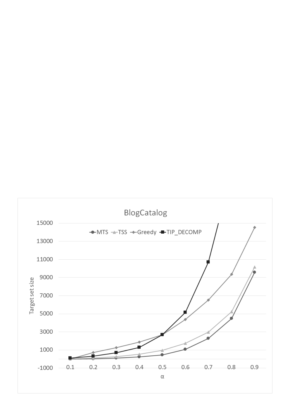
We present the results only for $10$ networks ( $4$ Directed and $6$ Undirected); the experiments performed on the other networks exhibit similar behaviors.

Analyzing the results from Figures 3-6, we notice that in all the considered cases our MTS algorithm always outperforms its competitors. The improvement is consistent with the results for random thresholds presented in the table 5. The differences in terms of performance of the algorithms, in this case, depend on two factors: the structural characteristics of the network and the thresholds. As noted previously, the largest differences are observed for intermediate values of the $\alpha$ parameter (for proportional thresholds) and for large values of the parameter $t$ , when these do not exceed the average degree of the nodes (for constant thresholds). In general, we provide the following observations:

•

the TSS algorithm provides performance close to MTS but the gap increases in the proportional threshold case, especially for intermediate values of the parameter $\alpha$ (see Fig. 7);
•

the Greedy algorithm performance improves with increasing thresholds;
•

the TIP_DECOMP performances worsen dramatically with increasing thresholds.

6.2 Correlation between Network Modularity and Normalized Target Set Size

Analyzing the results from Figures 3 to 6, we observe that the performance of the algorithms on different networks are influenced by the strength of communities of a network, measured by the modularity. Modularity is one measure of the structure of networks. Networks with high modularity have dense connections between the nodes within communities but sparse connections between nodes in different communities. In order to better evaluate the correlation between the modularity and the performances of the algorithms (measured considering the normalized target set size, which corresponds to the size of the target set, provided by the algorithm, divided by the number of nodes in the network), we measured the correlation using a statistical metric: the Pearson product-moment Correlation Coefficient (PCC). PCC is one of the measures of correlation which quantifies the strength as well as direction of the relationship between two variables. The correlation coefficient ranges from $-1$ (strong negative correlation) to $1$ (strong positive correlation). A value equal to $0$ implies that there is no correlation between the variables. We computed the correlation PCC between network modularity and normalized target set size, both with random and majority ( $\alpha=0.5$ ) thresholds. In particular, we considered two variables that are parametrized by the class N of Networks (see Table 4), the algorithm $A\in\{$ MTS, TSS, Greedy, TIP_DECOMP $\}$ , and the threshold function $F\in\{$ Random, Majority $\}$ . The variable $M(N)$ denotes the network modularity; the variable $T(N,A,F)$ denotes the normalized target set size. We observed that, in all the considered cases, there is a moderate positive correlation between modularity and normalized target set size (the PCC is between $0.5$ and $0.7$ ). Figure 8 presents the correlation values obtained. The reasoning behind those results is that when the network is composed by strongly connected components (high modularity), the influence hardly propagates from one community to another, thus the size of the target set increases. Figure 8 also shows that the correlation does not depend on the threshold function, while it is more sensible on the results provided by the algorithms TSS and MTS. This results is probably due to the fact that the algorithms TSS and MTS are able to better exploit situations where the community structure of the networks allows a certain influence between different communities.

We also performed similar analysis evaluating the correlation between the normalized target set size and the other network properties depicted in Table 4. Results show only a weak (the PCC is between $-0.5$ and $-0.3$ ) negative correlation between the average degree and the normalized target set size. In all the other cases the PCC is between $-0.3$ and $+0.3$ (there is none or very weak correlation).

7 Conclusion

We considered the problem of selecting a minimum size subset of nodes of a network which can start an activation process that spreads to all the nodes of the network. We presented a fast and simple algorithm that is optimal for several classes of graphs and matches the general upper bound given in [1, 17] on the cardinality of a minimum target set. Moreover, on real life networks, it outperforms the other known heuristics for the same problem. Experimental results show that the performance of all the analyzed algorithms correlates with the modularity of the analyzed network. This correlation is more sensible on the results provided by the MTS algorithm. This results is probably due to the fact that the proposed algorithms is able to better exploit situations when the community structure of the networks allows a certain influence between different communities.

There are many possible ways of extending our work. We would be especially interested in discovering additional interesting classes of graphs for which our algorithm is optimal or approximable within a small factor (with respect to the general $O(2^{\log^{1-\epsilon}|V|})$ inapproximability factor proved in [6]).

References

[1] Eyal Ackerman, Oren Ben-Zwi, and Guy Wolfovitz. Combinatorial model and bounds for target set selection. Theoretical Computer Science, 411(44–46):4017–4022, 2010.
[2] Cristina Bazgan, Morgan Chopin, André Nichterlein, and Florian Sikora. Parameterized approximability of maximizing the spread of influence in networks. Journal of Discrete Algorithms, 27:54–65, 2014.
[3] Oren Ben-Zwi, Danny Hermelin, Daniel Lokshtanov, and Ilan Newman. Treewidth governs the complexity of target set selection. Discrete Optimization, 8(1):87–96, 2011.
[4] Robert M. Bond, Christopher J. Fariss, Jason J. Jones, Adam D. I. Kramer, Cameron Marlow, Jaime E. Settle, and James H. Fowler. A 61-million-person experiment in social influence and political mobilization. Nature, 489:295–298, 2012.
[5] Carmen C. Centeno, Mitre C. Dourado, Lucia Draque Penso, Dieter Rautenbach, and Jayme L. Szwarcfiter. Irreversible conversion of graphs. Theoretical Computer Science, 412(29):3693–3700, 2011.
[6] Ning Chen. On the approximability of influence in social networks. SIAM Journal on Discrete Mathematics, 23(3):1400–1415, 2009.
[7] Wei Chen, Carlos Castillo, and Laks Lakshmanan. Information and Influence Propagation in Social Networks. Morgan & Claypool, 2013.
[8] Wei Chen, Chi Wang, and Yajun Wang. Scalable influence maximization for prevalent viral marketing in large-scale social networks. In Proceedings of the 16th ACM SIGKDD International Conference on Knowledge Discovery and Data Mining, pages 1029–1038, 2010.
[9] Wei Chen, Yajun Wang, and Siyu Yang. Efficient influence maximization in social networks. In Proceedings of the 15th ACM SIGKDD International Conference on Knowledge Discovery and Data Mining, KDD ’09, pages 199–208, New York, NY, USA, 2009.
[10] Chun-Ying Chiang, Liang-Hao Huang, Bo-Jr Li, Jiaojiao Wu, and Hong-Gwa Yeh. Some results on the target set selection problem. Journal of Combinatorial Optimization, 25(4):702–715, 2013.
[11] Chun-Ying Chiang, Liang-Hao Huang, and Hong-Gwa Yeh. Target set selection problem for honeycomb networks. SIAM Journal on Discrete Mathematics, 27(1):310–328, 2013.
[12] Morgan Chopin, André Nichterlein, Rolf Niedermeier, and Mathias Weller. Constant thresholds can make target set selection tractable. Theory of Computing Systems, 55(1):61–83, 2014.
[13] Nicholas A. Christakis and James H. Fowler. Connected: The Surprising Power of Our Social Networks and How They Shape Our Lives – How Your Friends’ Friends’ Friends Affect Everything You Feel, Think, and Do. Back Bay Books, reprint edition, January 2011.
[14] Ferdinando Cicalese, Gennaro Cordasco, Luisa Gargano, Martin Milanič, Joseph Peters, and Ugo Vaccaro. Spread of influence in weighted networks under time and budget constraints. Theoretical Computer Science, 586:40–58, 2015.
[15] Ferdinando Cicalese, Gennaro Cordasco, Luisa Gargano, Martin Milanič, and Ugo Vaccaro. Latency-bounded target set selection in social networks. Theoretical Computer Science, 535:1 – 15, 2014.
[16] Amin Coja-Oghlan, Uriel Feige, Michael Krivelevich, and Daniel Reichman. Contagious sets in expanders. In Proceedings of the Twenty-Sixth Annual ACM-SIAM Symposium on Discrete Algorithms, pages 1953–1987, 2015.
[17] Gennaro Cordasco, Luisa Gargano, Marco Mecchia, Adele A. Rescigno, and Ugo Vaccaro. A fast and effective heuristic for discovering small target sets in social networks. In Proc. of COCOA 2015, volume 9486, pages 193–208, 2015.
[18] Gennaro Cordasco, Luisa Gargano, Adele A. Rescigno, and Ugo Vaccaro. Optimizing Spread of Influence in Social Networks via Partial Incentives. In Structural Information and Communication Complexity: 22nd International Colloquium, SIROCCO 2015, pages 119–134. Springer International Publishing, 2015.
[19] Gennaro Cordasco, Luisa Gargano, Adele A. Rescigno, and Ugo Vaccaro. Brief announcement: Active information spread in networks. In Proceedings of the 2016 ACM Symposium on Principles of Distributed Computing, PODC ’16, pages 435–437, New York, NY, USA, 2016. ACM.
[20] Gennaro Cordasco, Luisa Gargano, Adele A. Rescigno, and Ugo Vaccaro. Evangelism in social networks. In Combinatorial Algorithms - 27th International Workshop, IWOCA 2016, Helsinki, Finland, August 17-19, 2016, Proceedings, pages 96–108, 2016.
[21] Gennaro Cordasco, Luisa Gargano, and Adele Anna Rescigno. Influence propagation over large scale social networks. In Proceedings of the 2015 IEEE/ACM International Conference on Advances in Social Networks Analysis and Mining, ASONAM 2015, Paris, France, pages 1531–1538, 2015.
[22] Thang N. Dinh, Huiyuan Zhang, Dzung T. Nguyen, and My T. Thai. Cost-effective viral marketing for time-critical campaigns in large-scale social networks. IEEE/ACM Trans. Netw., 22(6):2001–2011, December 2014.
[23] Pedro Domingos and Matt Richardson. Mining the network value of customers. In Proceedings of the Seventh ACM SIGKDD International Conference on Knowledge Discovery and Data Mining, KDD ’01, pages 57–66, New York, NY, USA, 2001.
[24] Paola Flocchini, Rastislav Královic, Peter Ruzicka, Alessandro Roncato, and Nicola Santoro. On time versus size for monotone dynamic monopolies in regular topologies. Journal of Discrete Algorithms, 1(2):129–150, 2003.
[25] Daniel Freund, Matthias Poloczek, and Daniel Reichman. Contagious sets in dense graphs. In Proceedings of 26th Int’l Workshop on Combinatorial Algorithms (IWOCA2015), 2015.
[26] Luisa Gargano, Pavol Hell, Joseph G. Peters, and Ugo Vaccaro. Influence diffusion in social networks under time window constraints. Theor. Comput. Sci., 584(C):53–66, 2015.
[27] Mark Granovetter. Threshold models of collective behavior. The American Journal of Sociology, 83(6):1420–1443, 1978.
[28] David Kempe, Jon Kleinberg, and Éva Tardos. Maximizing the spread of influence through a social network. Theory of Computing, 11(4):105–147, 2015.
[29] David Kempe, Jon Kleinberg, and Éva Tardos. Maximizing the spread of influence through a social network. In Proceedings of the Ninth ACM SIGKDD International Conference on Knowledge Discovery and Data Mining, KDD ’03, pages 137–146, New York, NY, USA, 2003.
[30] David Kempe, Jon Kleinberg, and Éva Tardos. Influential nodes in a diffusion model for social networks. In Proceedings of the 32Nd International Conference on Automata, Languages and Programming, ICALP’05, pages 1127–1138, Berlin, Heidelberg, 2005.
[31] Suman Kundu and Sankar K. Pal. Deprecation based greedy strategy for target set selection in large scale social networks. Information Sciences, 316:107–122, 2015.
[32] Matti Leppaniemi, Heikki Karjaluoto, Heikki Lehto, and Anni Goman. Targeting young voters in a political campaign: Empirical insights into an interactive digital marketing campaign in the 2007 finnish general election. Journal of Nonprofit & Public Sector Marketing, 22(1):14–37, 2010.
[33] Jure Leskovec, Lada A. Adamic, and Bernardo A. Huberman. The dynamics of viral marketing. ACM Trans. Web, 1(1), May 2007.
[34] Jure Leskovec and Andrej Krevl. SNAP Datasets: Stanford large network dataset collection. http://snap.stanford.edu/data, 2015.
[35] Mark Newman. Network data, http://www-personal.umich.edu/~mejn/netdata/, 2015.
[36] André Nichterlein, Rolf Niedermeier, Johannes Uhlmann, and Mathias Weller. On tractable cases of target set selection. Social Network Analysis and Mining, 3(2):233–256, 2013.
[37] T. V. Thirumala Reddy and C. Pandu Rangan. Variants of spreading messages. J. Graph Algorithms Appl., 15(5):683–699, 2011.
[38] Jean-Baptiste Rival and Joey Walach. The use of viral marketing in politics: A case study of the 2007 french presidential election. Master Thesis, Jönköping University, Jönköping International Business School.
[39] Paulo Shakarian, Sean Eyre, and Damon Paulo. A scalable heuristic for viral marketing under the tipping model. Social Network Analysis and Mining, 3(4):1225–1248, 2013.
[40] K. Tumulty. Obama’s viral marketing campaign. TIME Magazine, July 2007.
[41] Stanley Wasserman and Katherine Faust. Social Network analysis: Methods and Applications. Cambridge University Press, 1994.
[42] Reza Zafarani and Huan Liu. Social computing data repository at ASU. http://socialcomputing.asu.edu, 2009.
[43] Manouchehr Zaker. On dynamic monopolies of graphs with general thresholds. Discrete Mathematics, 312(6):1136–1143, 2012.

On Finding Small Sets that Influence Large Networks Thanks: A preliminary version of this paper was presented at the 1st International Workshop on Dynamics in Networks (DyNo 2015) in conjunction with the 2016 IEEE/ACM International Conference ASONAM, Paris, France, August 25-28, 2015. [21]

Abstract

1 Introduction

1.1 Our Results

2 The Minimum Target Set Problem

3 The MTS algorithm

Remark 1.

3.1 Algorithm Correctness

Fact 1.

Fact 2.

Lemma 1.

Proof.

Theorem 1.

Proof.

3.2 Running Time

4 Undirected graphs

4.1 Optimality on Trees, Cycles and Cliques

Theorem 2.

Example 1.

Lemma 2.

Proof.

Theorem 3.

Proof.

4.2 Optimality on Dense graphs

Theorem 4.

Proof.

Corollary 1.

4.3 Estimating the size of the solution for general graphs

Theorem 5.

Proof.

5 Directed graphs

5.1 DAGs

Theorem 6.

Proof.

5.2 Directed Trees.

Corollary 2.

5.3 Directed Cycles.

Theorem 7.

Proof.

6 Experimental results

6.1 Results

Random Thresholds.

Constant and Proportional thresholds.

6.2 Correlation between Network Modularity and Normalized Target Set Size

7 Conclusion

References

On Finding Small Sets that Influence
Large Networks Thanks: A preliminary version of this paper was presented at the 1st International Workshop on Dynamics in Networks (DyNo 2015) in conjunction with the 2016 IEEE/ACM International Conference ASONAM, Paris, France, August 25-28, 2015. [21]