Effective-one-body waveforms for binary neutron stars using surrogate models

In this work, we use the tidal EOB (TEOB) model developed in [47] and called $\text{TEOB}_{\text{Resum}}$. $\text{TEOB}_{\text{Resum}}$ incorporates an enhanced (resummed) attractive tidal potential derived from recent analytical advances in the PN and gravitational self-force description of relativistic tidal interactions [51, 52]. The resummed tidal potential of $\text{TEOB}_{\text{Resum}}$ significantly improves the description of tidal interactions near the merger over the previous next-next-to-leading-order (NNLO) TEOB model [53, 54] and over the conventional PN models. In particular, $\text{TEOB}_{\text{Resum}}$ predicts high-resolution, multi-orbit numerical relativity results within their uncertainties and without fitting parameters to BNS numerical waveforms [47].

The main features of $\text{TEOB}_{\text{Resum}}$ are summarised in what follows. The Hamiltonian is $H_{\rm EOB}=M\sqrt{1+2\nu(\hat{H}_{\rm eff}-1)}$ with

where the binary mass is $M=M_{A}+M_{B}$, the symmetric mass-ratio is $\nu=M_{A}M_{B}/M^{2}$, $u\equiv 1/r$, $r$ is the EOB radial coordinate, and $p_{\varphi}$ and $p_{r_{*}}$ are the conjugate momenta (see e.g. [53]). The EOB potential

is the sum of a point-mass term and a tidal term. $A_{0}(u;\nu)$ is defined as the $(1,5)$ Padé approximant of the formal 5PN expression $A_{0}^{\rm 5PN}(u;\nu)=1-2u+a_{3}u^{3}+a_{4}u^{4}+(a_{5}^{c}(\nu)+a_{5}^{\ln}\ln u)u^{5}+(a_{6}^{c}(\nu)+a_{6}^{\ln}\ln u)u^{6}$. The coefficients up to 4PN, i.e. $(a_{3},a_{4},a_{5}^{c}(\nu),a_{5}^{\ln})$, are analytically known [55]. Although the 5PN term $a_{6}^{\ln}$ and the linear-in-$\nu$ part of $a_{6}^{c}(\nu)$ are analytically known [56, 57], we use the value $a_{6}^{c}(\nu)=3097.3\nu^{2}-1330.6\nu+81.38$ fit to NR data in [58]. The tidal term,

models the gravito-electric sector of the interaction ¹¹ 1 The tidal interactions of a star (e.g. star A, we omit the labels in this footnote) in an external field are in general parametrized by (i) gravito-electric coefficients $G\mu_{\ell}$ $[length]^{2\ell+1}$ measuring the $\ell$th-order mass multipolar moment induced in the star by the external $\ell$th-order gravito-electric field; (ii) gravito-magnetic coefficients $G\sigma_{\ell}$ $[length]^{2\ell+1}$ measuring the $\ell$th-order spin multipolar moment induced in the star by the external $\ell$th-order gravito-magnetic field; (iii) shape coefficients $h_{\ell}$ measuring the distorsion of the surface of the star by an external $\ell$th-order gravito-electric field. In the literature, it is customary to consider only the dominant gravito-electric interactions (i) and, in most of the cases, only the leading order term $\ell=2$. The dimensionless Love numbers are defined as $k_{\ell}=(2\ell-1)!!G\mu_{\ell}/(2R^{2\ell+1})$, with $R$ the star radius. $\mu_{2}$ is simply called $\lambda$ in [96, 62, 65]. Other notations are employed in [65] ($\lambda\to\Lambda$) and in [67]., where

are the $\ell=2,3,4$ tidal polarizability paramaters (or tidal coupling constants) [51]. Labels $A,B$ refer to the stars, $M_{A}$ is the gravitational mass of star $A$, $R_{A}$ the areal radius, $C_{A}=M_{A}/R_{A}$, $X_{A}=M_{A}/M$, and $k_{\ell}^{A}$ are the dimensionless Love numbers [60, 53, 61, 62]. The expressions above assume $M_{A}\geq M_{B}$, so that $Q=M_{A}/M_{B}\geq 1$. In the equal-mass case, the tidal interaction and EOS information are fully encoded at leading order (LO) in the total dimensionless quadrupolar tidal coupling constant

The relativistic correction factors $\hat{A}^{(\ell^{+})}_{A}$ formally include all the high PN corrections to the leading-order. The particular choice of $\hat{A}^{(\ell^{+})}_{A}$ defines the TEOB model considered in this paper. The PN-expanded NNLO, fractionally 2PN accurate, expression is

with $\alpha^{(2),(3)}_{1,2}\neq 0$ computed analytically and $\alpha^{(4)}_{1,2}=0$ [63]. This $\text{TEOB}_{\text{NNLO}}$ model has been compared against NR simulations in [54, 47], significant deviations are observed at dimensionless GW frequencies $M\omega_{22}\gtrsim 0.8$, i.e. after contact and during the last 2-3 orbits to merger. The $\text{TEOB}_{\text{Resum}}$ model is defined from $\text{TEOB}_{\text{NNLO}}$ by substituting the $\ell=2$ term in (6) with the expression

where the functions $\tilde{A}_{1}^{(2^{+})\rm 1SF}(u)$ and $\tilde{A}_{2}^{(2^{+})\rm 2SF}(u)$ are given in [52] and $p=4$. The key idea of $\text{TEOB}_{\text{Resum}}$ is to use as pole location in Eq. (7) the light ring $r_{\rm LR}(\nu;\kappa_{A}^{(\ell)})\,$ of the $\text{TEOB}_{\text{NNLO}}$ model, i.e., the location of the maximum of $A^{\rm NNLO}(r;\,\nu;\,\kappa_{A}^{(\ell)})/r^{2}$. $\text{TEOB}_{\text{Resum}}$ is completed with a resummed waveform [64] that includes the NLO tidal contributions computed in [51, 65, 66].

A black hole limit of $\text{TEOB}_{\text{Resum}}$ is given by setting $\kappa^{(\ell)}_{A,B}\to 0$. Waveforms obtained this way, however, do not accurately represent BBH ones because the model does not include next-to-quasicircular corrections tuned to BBH NR data (so it actually differs from the model of [58]). For this reason we exclude the $\kappa^{(\ell)}_{A,B}=0$ configurations from the surrogate model. That is not a serious limitation because BBH waveform models are independently available, and because BBH sources are not expected in the mass range covered by our surrogate. Additionally, including the correct BBH limit would introduce a discontinuity in the waveform’s parameters space that would affect the overall accuracy of the surrogate. In a similar way, configurations with $\kappa^{(\ell)}_{B}\to 0$ approximate black hole-neutron star binaries, but with an astrophysically unexpected small mass ratio $Q$.

The $\text{TEOB}_{\text{Resum}}$ waveform model is determined by seven input parameters (7D parameter space): the binary mass-ratio $Q$ and the $\ell=2,3,4$ tidal polarizability paramaters (or tidal coupling constants) $\kappa^{A,B}_{\ell}$. The latter are linked to the usual multipolar dimensionless tidal parameters, e.g. [51, 67]. For each star we define

which are proportional to the $Q$-independent part of $\kappa^{A}_{\ell}$, and correspond to the multipolar quantities called $\bar{\lambda}_{\ell}$ in [67].

In constructing a surrogate, it is extremely important to reduce the dimensionality of the parameter space as much as possible in order to avoid high-dimensional interpolation which is often inaccurate and computationally demanding. Fortunately, Yagi has found tight correlations between the $\ell=2$ tidal parameter and the $\ell=3$ and $\ell=4$ tidal parameters that are nearly independent of the choice of EOS for plausible NS EOS models [67]. Yagi then constructed fits $\Lambda_{3}^{\rm fit}(\Lambda_{2})$ and $\Lambda_{4}^{\rm fit}(\Lambda_{2})$ for the $\ell=3$ and 4 tidal parameters in terms of the $\ell=2$ tidal parameter. This reduces the 7D parameter space

where $q=M_{B}/M_{A}\leq 1$ to the 3D parameter space

We evaluate the systematic uncertainty from these fits for 14 different EOS and for NS masses in the range $M\in[0.9M_{\odot},M_{\text{max}}]$, where $M_{\text{max}}$ is the maximum mass. For these EOS and masses, we find the $\ell=3$ fit $\Lambda_{3}^{\rm fit}(\Lambda_{2})$ results in fractional errors in the range $-0.098\leq\Delta\Lambda_{3}/\Lambda_{3}\leq 0.17$ with an average absolute fractional error of $\langle|\Delta\Lambda_{3}/\Lambda_{3}|\rangle=0.04$. The $\ell=4$ fit $\Lambda_{4}^{\rm fit}(\Lambda_{2})$ results in fractional errors in the range $-0.22\leq\Delta\Lambda_{4}/\Lambda_{4}\leq 0.28$ with an average absolute fractional error of $\langle|\Delta\Lambda_{4}/\Lambda_{4}|\rangle=0.08$. Details are given in the Appendix.

In Fig. 1, we show the contribution of each tidal effect to the phase evolution of the waveform for both the soft EOS SLY [68] and the stiff EOS MS1b [69]. (See [70] for the naming convention.) The phase shift due to the tidal interactions is usually $\sim 10$ radian for the $\ell=2$ interaction, $\sim 1$ radian for the $\ell=3$ interaction, and $\sim 0.1$ radian for the $\ell=4$ interaction for frequencies up to the maximum amplitude. Also shown is the typical error expected in the phase that results from using the fits $\Lambda_{3}^{\rm fit}(\Lambda_{2})$ and $\Lambda_{4}^{\rm fit}(\Lambda_{2})$ instead of the true values of $\Lambda_{3}$ and $\Lambda_{4}$ determined by the EOS. This error is smaller than the $\ell=4$ tidal effect with an overall error of $\lesssim 0.01$ radian.

When constructing a training set, significant care is required in choosing the waveform parameters as the choice made can impact the accuracy (and sometimes the ability) to accurately estimate or fit the waveform data in Step 3 above. We work in units for the mass parameters where the waveform amplitude and time samples are rescaled by the total mass $M=M_{A}+M_{B}$ so that a mass-ratio parameter is the only mass parameter needed for the surrogate. Three common choices are $q=M_{B}/M_{A}\leq 1$, $Q=M_{A}/M_{B}\geq 1$, and the symmetric mass ratio $\nu=M_{A}M_{B}/M^{2}\leq 1/4$. We have found that the symmetric mass ratio $\nu$ is a poor choice for $\text{TEOB}_{\text{Resum}}$ waveforms since the amplitude and phase at fixed times can sometimes change rapidly between grid points in the training set of parameters, which will make fitting for the parametric variation (see Step 3 above) difficult. The amplitude and phase vary less rapidly as functions of $q$ and $Q$, and we find that $q$ provides slightly better accuracy of the final surrogate model. We choose $q\in[0.5,1]$ as the mass ratio parameter.

For the tidal parameters, we use a rectangular grid of $\Lambda_{2}^{A}\in[50,5000]$ for the more massive NS and $\Lambda_{2}^{B}\in[50,5000]$ for the less massive NS. For any realistic EOS, $\Lambda_{2}^{B}\geq\Lambda_{2}^{A}$, so only a triangular half of this rectangular grid is physically plausible. However, because most implementations of accurate interpolation algorithms for multi-dimensional data require rectangular grids, we will sample the entire rectangular grid. Other choices for the two tidal parameters include $\kappa_{2}^{A}$ and $\kappa_{2}^{B}$ (defined in Eq. (4)), as well as $\tilde{\Lambda}$ and $\delta\tilde{\Lambda}$, which are another linear combination of $\Lambda_{2}^{A}$ and $\Lambda_{2}^{B}$ used in parameter estimation [14, 6]. Both of these alternative choices suffer from the same problem. In particular, mapping a rectangular grid of $\{\kappa_{2}^{A},\kappa_{2}^{B}\}$ or $\{\tilde{\Lambda},\delta\tilde{\Lambda}\}$ to the corresponding values of $\{\Lambda_{2}^{A},\Lambda_{2}^{B}\}$ can take $\Lambda_{2}$ outside the domain where the fits $\Lambda_{3}^{\rm fit}(\Lambda_{2})$ and $\Lambda_{4}^{\rm fit}(\Lambda_{2})$ (Eq. (31)) are valid. This makes it impossible to evaluate the $\ell=3,4$ tidal parameters.

With this choice of parameters,

we next choose a discretization of the parameter space to define the training set that will be used in Step 1. As discussed in Sec. III.4 below, we will use Chebyshev interpolation to fit for the variation of the amplitude and phase in terms of the waveform parameters ${\bm{\theta}}$. So, in constructing our training set, we choose waveform parameters at Chebyshev-Gauss-Lobatto nodes [72]. For each parameter, after linearly rescaling the range to $x\in[-1,1]$, the location of the $M$ nodes are given by

where $k=0,\dots,M-1$. We have found that a grid of $16\times 16\times 16=4096$ parameters, shown in Fig. 2, is sufficient to reach the desired accuracy of the final model. These $N=4096$ points define our training set of parameters, ${\cal T}_{N}:=\{{\bm{\theta}}_{i}\}_{i=1}^{N}$, that is used in building our surrogate model. This grid is more densely sampled at the edges of the parameter space, which is convenient because the algorithm we use for constructing the reduced basis (see Step 1) tends to choose parameters near the boundary of the training set. We then run the $\text{TEOB}_{\text{Resum}}$ code to generate 4096 waveforms at these training set parameter values with a starting frequency that is less than 10 Hz for any combination of parameters with $M_{A}\geq M_{B}\geq 1M_{\odot}$, which corresponds to a length of $\sim 2\times 10^{8}M$ in dimensionless units. This collection of waveforms constitutes our training data.

As discussed in Appendix E of Ref. [24], it is very helpful that the training set waveforms be accurately aligned at maximum amplitude. Otherwise, the amplitude and phase will not be smooth functions of the waveform parameters and the resulting surrogate model may not have a compact size, which automatically results in a loss of evaluation speed. We do this alignment by (i) densely sampling a waveform near the time of maximum amplitude, (ii) interpolating the amplitude with cubic splines, (iii) numerically finding the maximum of the interpolated amplitude, and (iv) shifting the waveform such that $t=0$ corresponds to the maximum amplitude. We then set the phase to zero at the common starting time for the shifted waveform. This alignment procedure is performed for all waveforms in the training data set.

Finally, we resample all of the training data waveforms to reduce the physical memory storage requirements. Before $t=-10^{3}M$, we sample the amplitude and phase uniformly in phase with a spacing of $\Delta\Phi=\pi$. After this time we use a uniform in time sampling with a spacing of $\Delta t=0.1M$ to capture the more complicated behavior near merger. This leads to waveforms that only require $\sim 7\times 10^{4}$ samples compared to $\gtrsim 10^{8}$ samples if we had sampled uniformly in time with sufficient accuracy to capture the behavior near merger. Our nonuniform downsampling allows us to store the entire waveform training data in $\sim 7$GB instead of many TB. More elaborate downsampling strategies exist including one that uses theoretically derived bounds on cubic spline errors to estimate the largest spacing between data points [30] and one that uses a greedy algorithm to select only those data points that are sufficient to recover the full data set up to a requested accuracy by a spline of a given, arbitrary degree [73, 74].

With the training set of waveforms in hand we now focus on reducing the data to its essential components in both parameters (this subsection) and time (in the next subsection). The reduction to a compact set of parameters can be achieved by building a reduced basis such that the projection ${\cal P}$ of any training set waveform onto the basis will be indistinguishable from the original waveform up to some tolerance that is specified. We build a reduced basis using a greedy algorithm [25, 26, 27, 28], which exposes the most relevant parameters in the training set that capture the salient features of the waveform training data.

The greedy algorithm we use is given in [24], to which we refer the reader for further details, and shown in Alg. 1. The algorithm terminates after $n$ iterations when the projection error is smaller than a specified tolerance $\epsilon$. The output of the greedy algorithm includes a set of parameter tuples $\{{\bm{\mu}}_{i}\}_{i=1}^{n}$, sometimes called greedy parameters or greedy points, and a reduced basis $\{e_{i}(t)\}_{i=1}^{n}$. We use the symbol $X$ as a place holder for a waveform variable. In Alg. 1 and throughout, $||\cdot||^{2}=\langle\cdot,\cdot\rangle$ is the squared $L_{2}$ norm where

is the integral of the product of two generally complex functions $f(t)$ and $g(t)$ and is sometimes called an inner product.

To make the reduced basis as compact as possible, we follow [24, 30, 34, 31] and represent the complex waveforms by their amplitudes and phases instead of real and imaginary parts. We then build a separate reduced basis for each of the amplitude and phase training data. This decomposition is made because the amplitude and phase of a waveform have less variation and features in both time and parameters than do the real and imaginary parts of the waveform, which have many oscillations. The greedy algorithm is sensitive to waveform morphologies and will tend to increase the size of the reduced basis in order to resolve these structures. As a result, using an amplitude and phase representation for the waveform allows, in our case, for an extremely compact pair of bases.

We executed the greedy algorithm separately on the amplitudes and the phases of the training set waveforms. In practice, we use an iterated, modified Gram-Schmidt process [75], which is known to be robust against the accumulation of numerical round-off, to generate the orthogonal basis vectors in line 9 of Alg. 1. We chose relative tolerances of $\epsilon=10^{-10}$ and $10^{-15}$ for the amplitude and phase, respectively. We found that this resulted in extremely compact reduced basis sizes of $n_{A}=12$ for amplitudes and $n_{\Phi}=7$ for phases. These 12 and 7 greedy parameters are the minimal amount of information needed to represent the entire training set of $\text{TEOB}_{\text{Resum}}$ waveform amplitudes and phases, respectively, to within our chosen tolerances, as measured with the squared $L_{2}$ norm. Mathematically, if $A$ and $\Phi$ denote the amplitude and phase of a waveform and if $\{e_{i}^{A}(t)\}_{i=1}^{12}$ and $\{e_{i}^{\Phi}(t)\}_{i=1}^{7}$ are their corresponding reduced bases then

where the coefficients are

The orthonormal reduced basis elements for the phase are shown in Fig. 3. For comparison, if we had constructed a reduced basis for the complex waveform itself then the basis size would be several hundred to reach a maximum projection error of $10^{-10}$ across the entire training set of waveforms. The choice to decompose the waveforms into amplitude and phase is thus justified here.

The reduced basis greedy algorithm depends on a choice of seed, which is arbitrarily selected. The resulting sequence of parameter tuples selected by the greedy algorithm will depend on that choice of seed. A different choice still produces a reduced basis that represents all of the training data to within the specified tolerance, by construction. However, the sizes of the reduced bases built from different seeds tend to vary but will often lie within a few percent of each other so that the seed choice is immaterial [29, 73]. What matters is that we have a compact reduced basis to represent accurately the waveform amplitude and phase training data.

Greedy algorithms are extremely flexible for incorporating many decisions and choices for building a reduced-order model. For example, in a greedy algorithm one can measure the projection errors with the $L_{2}$ norm, as we did here, or with the $L_{\infty}$ norm to provide a more stringent requirement of the reduced basis to represent the data in a point-wise sense. Other problem-specific error measures may be more appropriate (e.g., see [40]). One may also implement different greedy algorithms strategies for very large training spaces. For example, the training set can be randomly resampled at every iteration of the greedy algorithm, as described in [40]. Yet another strategy is to parallelize the computation of the inner product integrals used to compute the projections onto the reduced basis [76].

The reduced basis representations of the amplitude and phase in (14) require knowing the coefficients in (15) or, equivalently, the data $A(t;{\bm{\theta}})$ and $\Phi(t;{\bm{\theta}})$ that one is projecting onto the basis. We wish to predict these coefficients in the linear representations. One way to do this is to simply fit for the parametric dependence (i.e., ${\bm{\theta}}$) of the coefficients themselves [30, 31]. However, the ${\bm{\theta}}$ dependence of the coefficients can become increasingly noisy as the index $i$ increases, which can make the fits unreliable and the ensuing surrogate model evaluations not meet stringent accuracy requirements at new parameter values [77, 24].

The second step of surrogate building aims to provide a sparse subset of times from which it is possible to reconstruct the waveform at any other time by using an empirical interpolant [32], which is informed by the structure and features of $\text{TEOB}_{\text{Resum}}$ waveforms via the reduced basis found in Step 1. As we will discuss in the next subsection, fitting for the ${\bm{\theta}}$ dependence of the coefficients is done at each of these time subsamples, which are called empirical interpolation nodes. The data being fitted turn out to be robust to the gradual appearance of round-off noise, unlike fitting directly for the projection coefficients mentioned in the previous paragraph [24].

The algorithm for building an empirical interpolant is given in [24], to which we refer the reader for further details, and shown in Alg. 2. The empirical interpolant is built from a second greedy algorithm and proceeds as follows [33]. (We focus the presentation on the waveform amplitude for clarity but the same steps are taken for the phase.) First, we choose a value of time $\tau_{1}$ from the discrete set of available time samples $t:=\{t_{i}\}_{i=1}^{L}$ where $L$ is the number of samples. In our case, we mentioned in Sec. III.1 that our data have $L=7\times 10^{4}$ time samples that are nonuniformly distributed. This first time subsample $\tau_{1}$ is a seed for this greedy algorithm. In practice, for reasons of conditioning, one chooses the seed to be the time sample at which the first reduced basis function $e_{1}(t)$ is a maximum in absolute value so that $\tau_{1}={\rm arg~max}_{t}|e_{1}(t)|$. We follow this convention here.

For the next step, we build an empirical interpolant. We label the empirical interpolant ${\cal I}$ of a function $A(t;{\bm{\theta}})$ by the number $m$ of time subsamples we currently have, namely, ${\cal I}_{m}[A](t;{\bm{\theta}})$. The notation here is to indicate that ${\cal I}_{m}$ is an operator that acts on a function $A(t;{\bm{\theta}})$. If the function is independent of ${\bm{\theta}}$ then so will the interpolant’s operation on that function.

Currently, $m=1$ and we represent the interpolant as a linear combination of the first $m$ reduced basis elements so that

We assume that the empirical interpolant can always be written in affine form where the dependence on parameters ${\bm{\theta}}$ and time $t$ is factorized. To solve for the unknown coefficient $C_{1}({\bm{\theta}})$ in (16) we demand that the interpolant reproduce the data at $t=\tau_{1}$ so that ${\cal I}_{1}[A](t;{\bm{\theta}})=A(t;{\bm{\theta}})$. The solution is easily found and given by $C_{1}({\bm{\theta}})=A(\tau_{1};{\bm{\theta}})/e_{1}(\tau_{1})$ and the empirical interpolant so far is given by

where $B_{1}(t)=e_{1}(t)/e_{1}(\tau_{1})$. In operator form, the $m=1$ empirical interpolant is ${\cal I}_{1}[\cdot]=B_{1}(t)(\,\cdot\,|_{t=\tau_{1}})$.

The second empirical interpolant node $\tau_{2}$ is the time subsample at which the next reduced basis element $e_{2}(t)$ and its interpolation with the current interpolant ${\cal I}_{1}[e_{2}](t)$ is largest in absolute value,

Notice that we are choosing the next time subsample in an effort to improve the empirical interpolant’s point-wise representation of the reduced basis elements themselves. Recall that the reduced basis is all that is needed to accurately span the (training set of) waveforms. The set of nodes is now $\{\tau_{1},\tau_{2}\}$ and

is the empirical interpolant at this step. The coefficients are found as in usual interpolation problems. At the interpolation nodes $\{\tau_{1},\tau_{2}\}$ we require that (19) equals to the data $A(\tau_{i};{\bm{\theta}})$ and then solve the linear equation

where $V_{ji}:=e_{i}(\tau_{j})$, which are the elements of a Vandermonde matrix. After finding the solution, the $m=2$ empirical interpolant is

where $B_{j}(t)=\sum_{j=1}^{2}e_{i}(t)(V^{-1})_{ij}$ for $i=1,2$.

This process is repeated until we have used all $n$ of the reduced basis elements to build the final empirical interpolant,

where

is the $j^{\rm th}$ element of the empirical interpolation operator ${\bm{B}}$. In operator form, the empirical interpolant is

Notice that ${\bm{B}}$ in (23) is independent of the parameter ${\bm{\theta}}$ and can be computed off-line once the reduced basis is built in Step 1. The quantities $\{\tau_{j}\}_{j=1}^{n}$ are the corresponding interpolation nodes. In addition, the parameter dependence of the empirical interpolant depends on how the function $A$ varies only at the nodes $\{\tau_{j}\}_{j=1}^{n}$. Finally, notice that, given a parameter tuple ${\bm{\theta}}$, one still needs to know the actual values of the $\{A(\tau_{j};{\bm{\theta}})\}_{j=1}^{n}$ in order to compute the empirical interpolant in (22). We will show how surrogate modeling addresses this issue in Sec. III.4.

We applied this greedy algorithm to build an empirical interpolant separately for the waveform amplitude and phase, which are given by

The interpolating functions for the phase are shown in Fig. 4. The empirical interpolation nodes $\{\tau^{\Phi}_{j}\}_{j=1}^{7}$ are not uniformly spaced because they depend on the underlying features of the $\text{TEOB}_{\text{Resum}}$ waveform family.

The empirical interpolation greedy algorithm we just described and used in this paper is not optimized for speed. As discussed in Appendix B of [45], the original (discrete) empirical interpolation method algorithm proposed in [33], which is the one we discussed above, has a computational cost at the $m^{\rm th}$ step of the greedy algorithm that scales as ${\cal O}(m^{4})$. However, this relatively slow evaluation time is immaterial for our surrogate since the sizes of the amplitude ($n_{A}=12)$ and phase ($n_{\Phi}=7$) reduced bases are very small. A faster algorithm was put forward in [45] (see Algorithm 5 in their Appendix A) and was used in describing the reduced-order surrogate modeling strategy in [24]. This faster implementation has a cost that scales as ${\cal O}(m^{3})$ [45]. The computational savings with this faster algorithm is particularly useful for problems involving a large reduced basis, such as the reduced-order model built in [44] for the IMRPhenomPv2 waveform family [78] that contained at most $1253$ basis elements.

The last step in building the surrogate model is to estimate the ${\bm{\theta}}$ dependence at each of the empirical interpolation nodes for both the waveform amplitude and phase data. Because the parameter space is three dimensional, we intentionally selected our training points in Sec. III.1 to correspond to the nodes of Chebyshev interpolation in three dimensions. Chebyshev interpolation, which for smooth $C^{\infty}$ functions, has errors that converge exponentially with the number of Chebyshev polynomials $T_{n}(x)$ [72]. The amplitude and phase at each empirical interpolation node are approximated as a tensor product of Chebyshev polynomials,

for $j=1,\ldots n_{X}$ and $X=\{A,\Phi\}$. Although it would be possible to optimize the number of coefficients for each node $\tau_{j}$, for simplicity we use all $16\times 16\times 16$ coefficients at each node. The summations are efficiently performed using Clenshaw summation [79]. The coefficients $a_{j,lmn}$ and $b_{j,lmn}$ of the Chebyshev series are precomputed from the known amplitudes and phases on the training set grid using Gaussian quadrature [72]. This quadrature is efficiently performed using a type-I discrete cosine transform [80].

The required fractional accuracy of the interpolation is the maximum allowed amplitude or phase error divided by the range of values that the amplitude or phase takes at each empirical node $\tau_{j}$ over the training set. This is most stringent for the phase where, near the merger, we would like the error to be $\lesssim 0.1$ radians but the spread is $\sim 10^{3}$ radians over the considered parameter space. This requires a fractional accuracy of $\sim 10^{-4}$ for the interpolation. We assess the errors in the surrogate model due to interpolation in Sec. IV.1.

A distinct advantage of reduced-order surrogate models is that the data output from a simulation or code is used directly for building the model. The first steps (building a reduced basis and and empirical interpolant) are accomplished off-line using only the training data generated by the $\text{TEOB}_{\text{Resum}}$ code. The only model inputs come in the last step when we estimate the parameter dependence of the data at the empirical interpolation nodes because we implement a choice of fitting functions that can affect the resulting quality of the surrogate predictions. This often results in a surrogate that nearly retains the accuracy of the underlying training data used to build the model. In addition, propagating the training data uncertainties and assessing the surrogate errors is fairly straightforward because of the minimal amount of modeling inputs, which are isolated to Step 3. An example of this is given in [34] where a reduced-order surrogate model is built for the gravitational waveforms of non-spinning BBH coalescences produced by numerical relativity simulations.

After Step 3, the surrogate model for the amplitude and phase is defined by evaluating the corresponding empirical interpolant in (25) using the parametric estimations in (26) to predict the values at any new parameter values,

The surrogate evaluation is performed online once a parameter tuple $(q,\Lambda_{2}^{A},\Lambda_{2}^{B})$ is given.

In practical gravitational wave data analysis applications, one rescales from geometric units to physical units of time and amplitude. This rescaling also depends on the total mass $M$ of the compact binary. In addition, one specifies a starting frequency $f_{\rm start}$. The starting time $t_{\rm start}$ corresponding to $f_{\rm start}$ is calculated by numerically solving $f_{\rm start}=f(t_{\rm start})$, where $f(t)=(d\Phi_{S}/dt)/(2\pi)$ is the frequency once given a tuple of parameter values $(q,\Lambda_{2}^{A},\Lambda_{2}^{B})$. We then perform the necessary time and phase shifts and resample the amplitude and phase surrogate predictions in (27). The final expression for the surrogate model waveforms takes the form

where $\iota$ is the binary inclination angle and $d$ is the distance to the gravitational wave source.

In this paper, we have built a surrogate model for the amplitude and phase of $\text{TEOB}_{\text{Resum}}$ waveforms in the time domain. This surrogate approximates the waveform in a nonlinear representation (because the dependence on phase is nonlinear) and, as such, cannot be used directly for speeding up likelihood computations in parameter estimation studies [42, 43, 44] that use reduced-order quadratures [45]. However, it is straightforward to use our surrogate to build a new surrogate for this purpose in the following way. As we will discuss in the next section, our surrogate accurately predicts waveforms output by the TEOBresum code. As such, we may use the surrogate above to generate a new training set in $h_{+}$ and $h_{\times}$ form, which is a linear representation. Then, one can repeat the surrogate building Steps 1–3 for the two waveform polarizations directly. As mentioned earlier, this would generate reduced basis sizes that contain a few hundred elements and so would be somewhat larger in physical memory size and slower to evaluate the resulting surrogate. Furthermore, one could do this in the frequency domain by computing Fourier transforms of the time-domain training waveforms generated by the surrogate in (28) so that the transformation is part of the offline stage. One may still use our time domain surrogate presented here for parameter estimation studies but we expect significant speed-ups could be obtained by following the strategy just outlined for likelihood computations.

The required accuracy of the surrogate is determined by the smallest effect that we want to model. For BNS systems, this is the tidal interaction that effects the waveform by $\sim 10$ radians up to merger for typical EOSs. This means that we will require the waveform error to be significantly smaller than $\sim 10$ radians.

The accuracy of the surrogate can be assessed by comparing it to the training set used to construct the reduced basis as well as to a large set of waveforms with randomly sampled parameters. Fig. 5 shows the fractional error in the amplitude as well as the error in the phase between the surrogate waveform and each of the 4096 training set waveforms. The difference between the surrogate and each training set waveform is maximized over all times. For clarity we suppress the third paramater $\Lambda_{2}^{B}$ and only show the maximum error for the 16 values of $\Lambda_{2}^{B}$ at each grid point. The maximum fractional error in amplitude is $\Delta A/A=7.7\times 10^{-5}$, and the maximum error in phase is $\Delta\Phi=0.014$ radians. Because the interpolated values of $A$ and $\Phi$ exactly match the training set at each grid point at the empirical nodes $\tau_{j}$, we see from  (27) that the error in reproducing each training set waveform is due almost entirely to the finite number of reduced bases.

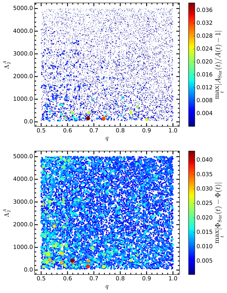
To determine how well the surrogate reproduces a generic waveform within the parameter space, we produce $10^{4}$ waveforms with parameters randomly sampled in the range $q\in[0.5,1]$, $\Lambda_{2}^{A}\in[50,5000]$, and $\Lambda_{2}^{B}\in[50,5000]$. The fractional amplitude and phase errors in reproducing the generic waveforms are shown in Fig. 6. The errors are maximized over time for each waveform. We find a maximum fractional amplitude error of $\Delta A/A=0.038$, but note that, prior to the last $100M$ before merger, the maximum error is $\Delta A/A=4\times 10^{-4}$, about two orders of magnitude smaller. The maximum phase error is $\Delta\Phi=0.043$ radians. For both the amplitude and phase, the error is largest for small values of the parameters. This results because both the amplitude and phase vary most rapidly for small values of the waveform parameters, so the interpolation of the amplitude $A(\tau^{A}_{j};q,\Lambda_{2}^{A},\Lambda_{2}^{B})$ and phase $\Phi(\tau^{\Phi}_{j};q,\Lambda_{2}^{A},\Lambda_{2}^{B})$ at each empirical node $\tau_{j}$ is least accurate there.

In Fig. 7, we show the last $10^{3}M$ of the $\sim 10^{8}M$ long waveform that is reproduced by the surrogate with the largest phase error. The phase error typically increases gradually with time. On the other hand, the amplitude error increases dramatically during the last cycle, and is typically two orders of magnitude smaller before the last cycle. This increase in error near the maximum amplitude likely results from the finite accuracy with which the training set waveforms are numerically aligned at maximum amplitude where the amplitude changes more rapidly with time, making accurate interpolation more difficult.

As a final check of the surrogate model accuracy, we examine the mismatch between the surrogate model and the original EOB waveform. The mismatch represents the loss in signal-to-noise ratio that would result from using the surrogate model instead of the original EOB waveform. It is defined by the deviation from a perfect overlap after aligning the two waveforms using the time and phase free parameters $t_{0}$ and $\phi_{0}$:

The inner product here is the integral of the Fourier transformed waveforms $\tilde{h}(f)$ weighted by the noise power spectral density (PSD) $S_{n}(f)$ of the detector:

In Fig. 8, we show the distribution of mismatch $\mathcal{M}$ between our surrogate and the $10^{4}$ randomly sampled EOB waveforms. We use the design sensitivity aLIGO PSD [81] and a sampling rate of 4096 Hz. Our integration bounds are $f_{\rm low}=30$ Hz and the Nyquist frequency $f_{\rm high}=2048$ Hz. Because the surrogate can be rescaled with mass, we show results for the smaller mass $M_{B}$ fixed at $1M_{\odot}$ or fixed at $2M_{\odot}$. The mismatch is larger for the higher mass systems because the frequency where the waveform ends scales inversely with the total mass, resulting in the less accurate end of the waveform occurring at smaller frequencies where the detector is more sensitive. Overall, the mismatch is typically smaller than $\sim 10^{-4}$ except for systems with large component masses, and the mismatch never exceeds $7\times 10^{-4}$.

One of the main purposes for generating a surrogate is to make parameter estimation more computationally efficient. In particular, parameter estimation codes, usually based on Markov Chain Monte Carlo or Nested Sampling, typically require $10^{7}$–$10^{8}$ sequential waveform evaluations, and the computational time is dominated by the waveform evaluation time even for PN waveforms [82, 83]. Recently, a few parallel algorithms have become available [84, 85]. However, the performance of these algorithms still scales linearly with the performance of the waveform generator.

We have produced a prototype Python implementation of our surrogate and a C implementation in the LIGO Algorithm Library (LAL) [86] under the name $\text{TEOB}_{\text{Resum}}$_ROM which is about 2 times faster than the Python version. The performance of the LAL implementation is shown in Fig. 9. For each waveform evaluation, there is a flat cost of $\sim 0.04$ s to calculate the amplitude and phase of the waveform at the $\sim 7\times 10^{4}$ samples using Eq. (27). The difference in evaluation time as the starting frequency $f_{\rm start}$ is varied results from the resampling of the amplitude and phase at evenly spaced times in Eq. (28). The number of these samples increases rapidly as the starting frequency is decreased. Most parameter estimation is done at 4096 Hz with a starting frequency of 30 Hz down to 10 Hz. The total waveform evaluation time will therefore be about 0.07 s up to 0.8 s. If necessary, the resampling of the amplitude and phase, which is the bottleneck for low starting frequencies, can be parallelized. The original implementation of the EOB code in Matlab can take $\sim 20$ minutes to evaluate, so this represents a speed-up factor of $10^{3}$–$10^{4}$ in some cases. However, it is not possible to make a direct comparison since the original Matlab code calculates a non-uniformly sampled waveform with units rescaled by the distance and mass.

As an end-to-end test of the surrogate, we inject a waveform into simulated aLIGO data and estimate its parameters using a Nested Sampling algorithm as implemented in LAL [87, 88, 89, 90]. Although EOB waveforms have been used in Bayesian parameter estimation for BBH systems which have significantly fewer cycles (e.g. [91]), this is one of the first times EOB waveforms have been used in a Bayesian analysis for BNS systems. Another analysis using a parallelized algorithm [85] is in progress [92].

The synthetic data are taken to be stationary and Gaussian, with a PSD corresponding to the aLIGO final design sensitivity [81]; two detectors are assumed, located at the Hanford and Livingston sites. For the simulated signal we choose an arbitrary sky position and orientation, a distance of 87 Mpc, and component masses $(M_{A},M_{B})=(1.4,1.4)\,M_{\odot}$. The EOS is taken to be MS1b, so that for the given masses one has $\Lambda_{2}^{A}=\Lambda_{2}^{B}=1286$ [7]. For the parameter choices made, the optimal signal-to-noise ratio is 26.28.

For the parameter estimation, the prior densities for sky position as well as orientation are chosen to be uniform on the sphere, and the distance prior is uniform in co-moving volume with an upper cut-off at 100 Mpc. Component masses are uniform in the interval $[1,2]\,M_{\odot}$, and we take $\Lambda_{2}^{A}$, $\Lambda_{2}^{B}$ to be uniform in the interval $[50,5000]$. In the Nested Sampling we use 512 live points and up to 5000 MCMC points [89], leading to $10^{7}-10^{8}$ likelihood evaluations; results from 4 different sampling chains are combined. Since the tidal effects we are interested in manifest themselves predominantly at high frequency, for this first exploration we use a lower cut-off frequency of 40 Hz; the sampling rate is 4096 Hz.

Since $\Lambda_{2}^{A}$ and $\Lambda_{2}^{B}$ are highly correlated, after the Nested Sampling algorithm has finished we change parameters to the $\tilde{\Lambda}$, $\delta\tilde{\Lambda}$ introduced in [6], which depend on $(q,\Lambda_{2}^{A},\Lambda_{2}^{B})$; note that these have the convenient properties $\tilde{\Lambda}(q=1,\Lambda_{2}^{A}=\Lambda_{2}^{B}=\Lambda)=\Lambda$ and $\delta\tilde{\Lambda}(q=1,\Lambda_{2}^{A}=\Lambda_{2}^{B}=\Lambda)=0$.

Posterior density functions for $\tilde{\Lambda}$ and $\delta\tilde{\Lambda}$ are shown in Fig. 10; both these parameters are recovered quite well. The parameter estimation code ran for 15 days; without a surrogate it would have taken well over a year.

Finally, as shown in [5, 8, 7], if the functional dependence of $\Lambda_{2}^{A}$, $\Lambda_{2}^{B}$ on component masses is expressed in terms of observables that can be expected to take approximately the same values for all sources, then posterior density functions for the latter can be trivially combined across detections to arrive at a more accurate measurement. These observables could be coefficients in a Taylor expansion [5, 8], or the parameters in a representation of the EOS in terms of piecewise polytropes [7]. An implementation for the surrogate model presented in this paper is left for future work.

References

- [1] G. M. Harry and LIGO Scientific Collaboration, Class. Quantum Grav. 27, 084006 (2010).
- [2] F. Acernese, et al. (Virgo Collaboration), “Advanced virgo baseline design, VIR-027A-09,” (2009).
- [3] K. Somiya, Class. Quantum Grav. 29, 124007 (2012), arXiv:1111.7185 [gr-qc] .
- [4] B. Iyer, T. Souradeep, C. S. Unnikrishnan, S. Dhurandhar, S. Raja, and A. Sengupta, LIGO Document M1100296-v2 (2011).
- [5] W. Del Pozzo, T. G. F. Li, M. Agathos, C. Van Den Broeck, and S. Vitale, Phys. Rev. Lett. 111, 071101 (2013), arXiv:1307.8338 [gr-qc] .
- [6] L. Wade, J. D. E. Creighton, E. Ochsner, B. D. Lackey, B. F. Farr, T. B. Littenberg, and V. Raymond, Phys. Rev. D 89, 103012 (2014).
- [7] B. D. Lackey and L. Wade, Phys. Rev. D 91, 043002 (2015), arXiv:1410.8866 [gr-qc] .
- [8] M. Agathos, J. Meidam, W. Del Pozzo, T. G. F. Li, M. Tompitak, J. Veitch, S. Vitale, and C. Van Den Broeck, Phys. Rev. D 92, 023012 (2015), arXiv:1503.05405 [gr-qc] .
- [9] K. Chatziioannou, N. Cornish, A. Klein, and N. Yunes, Astrophys. J. Lett. 798, L17 (2015), arXiv:1402.3581 [gr-qc] .
- [10] T. Damour, B. R. Iyer, and B. S. Sathyaprakash, Phys. Rev. D 63, 044023 (2001), gr-qc/0010009 .
- [11] A. Buonanno, B. R. Iyer, E. Ochsner, Y. Pan, and B. S. Sathyaprakash, Phys. Rev. D 80, 084043 (2009), arXiv:0907.0700 [gr-qc] .
- [12] J. Veitch, V. Raymond, B. Farr, W. Farr, P. Graff, S. Vitale, B. Aylott, K. Blackburn, N. Christensen, M. Coughlin, W. Del Pozzo, F. Feroz, J. Gair, C.-J. Haster, V. Kalogera, T. Littenberg, I. Mandel, R. O’Shaughnessy, M. Pitkin, C. Rodriguez, C. Röver, T. Sidery, R. Smith, M. Van Der Sluys, A. Vecchio, W. Vousden, and L. Wade, Phys. Rev. D 91, 042003 (2015), arXiv:1409.7215 [gr-qc] .
- [13] T. Hinderer, B. D. Lackey, R. N. Lang, and J. S. Read, Phys. Rev. D 81, 123016 (2010), arXiv:0911.3535 [astro-ph.HE] .
- [14] M. Favata, Phys. Rev. Lett. 112, 101101 (2014), arXiv:1310.8288 [gr-qc] .
- [15] K. Yagi and N. Yunes, Phys. Rev. D 89, 021303 (2014), arXiv:1310.8358 [gr-qc] .
- [16] A. Buonanno and T. Damour, Phys. Rev. D 59, 084006 (1999), arXiv:gr-qc/9811091 .
- [17] T. Damour and A. Nagar, Phys. Rev. D 81, 084016 (2010), arXiv:0911.5041 [gr-qc] .
- [18] Y. Pan, A. Buonanno, M. Boyle, L. T. Buchman, L. E. Kidder, H. P. Pfeiffer, and M. A. Scheel, Phys. Rev. D 84, 124052 (2011), arXiv:1106.1021 [gr-qc] .
- [19] A. Taracchini, Y. Pan, A. Buonanno, E. Barausse, M. Boyle, T. Chu, G. Lovelace, H. P. Pfeiffer, and M. A. Scheel, Phys. Rev. D 86, 024011 (2012), arXiv:1202.0790 [gr-qc] .
- [20] A. Taracchini, A. Buonanno, Y. Pan, T. Hinderer, M. Boyle, D. A. Hemberger, L. E. Kidder, G. Lovelace, A. H. Mroué, H. P. Pfeiffer, M. A. Scheel, B. Szilágyi, N. W. Taylor, and A. Zenginoglu, Phys. Rev. D 89, 061502 (2014), arXiv:1311.2544 [gr-qc] .
- [21] T. Damour, A. Nagar, and S. Bernuzzi, Phys. Rev. D 87, 084035 (2013), arXiv:1212.4357 [gr-qc] .
- [22] A. Nagar, T. Damour, C. Reisswig, and D. Pollney, Phys. Rev. D 93, 044046 (2016), arXiv:1506.08457 [gr-qc] .
- [23] C. Devine, Z. B. Etienne, and S. T. McWilliams, Classical and Quantum Gravity 33, 125025 (2016), arXiv:1601.03393 [astro-ph.HE] .
- [24] S. E. Field, C. R. Galley, J. S. Hesthaven, J. Kaye, and M. Tiglio, Phys. Rev. X 4, 031006 (2014), arXiv:1308.3565 [gr-qc] .
- [25] T. H. Cormen, C. Stein, R. L. Rivest, and C. E. Leiserson, Introduction to Algorithms, 2nd ed. (McGraw-Hill Higher Education, 2001).
- [26] P. Binev, A. Cohen, W. Dahmen, R. DeVore, G. Petrova, and P. Wojtaszczyk, SIAM Journal on Mathematical Analysis 43, 1457 (2011).
- [27] R. DeVore, G. Petrova, and P. Wojtaszczyk, (2012), 1204.2290 [math.FA] .
- [28] J. S. Hesthaven, B. Stamm, and S. Zhang, ESAIM: Mathematical Modelling and Numerical Analysis 48, 259 (2014).
- [29] S. E. Field, C. R. Galley, F. Herrmann, J. S. Hesthaven, E. Ochsner, et al., Phys. Rev. Lett. 106, 221102 (2011), arXiv:1101.3765 [gr-qc] .
- [30] M. Pürrer, Class. Quantum Grav. 31, 195010 (2014), arXiv:1402.4146 [gr-qc] .
- [31] M. Pürrer, Phys. Rev. D 93, 064041 (2016), arXiv:1512.02248 [gr-qc] .
- [32] M. Barrault, Y. Maday, N. C. Nguyen, and A. T. Patera, Comptes Rendus Mathematique 339, 667 (2004).
- [33] S. Chaturantabut and D. C. Sorensen, SIAM Journal on Scientific Computing 32, 2737 (2010).
- [34] J. Blackman, S. E. Field, C. R. Galley, B. Szilágyi, M. A. Scheel, M. Tiglio, and D. A. Hemberger, Phys. Rev. Lett. 115, 121102 (2015), arXiv:1502.07758 [gr-qc] .
- [35] C. R. Galley, F. Herrmann, J. Silberholz, M. Tiglio, and G. Guerberoff, Class. Quantum Grav. 27, 245007 (2010), arXiv:1005.5560 [gr-qc] .
- [36] K. Cannon, A. Chapman, C. Hanna, D. Keppel, A. C. Searle, and A. J. Weinstein, Phys. Rev. D 82, 044025 (2010), arXiv:1005.0012 [gr-qc] .
- [37] K. Cannon, C. Hanna, and D. Keppel, Phys. Rev. D 84, 084003 (2011), arXiv:1101.4939 [gr-qc] .
- [38] S. E. Field, C. Galley, and E. Ochsner, Phys. Rev. D 86, 084046 (2012), arXiv:1205.6009 [gr-qc] .
- [39] S. Caudill, S. E. Field, C. R. Galley, F. Herrmann, and M. Tiglio, Class. Quantum Grav. 29, 095016 (2012), arXiv:1109.5642 [gr-qc] .
- [40] J. Blackman, B. Szilagyi, C. R. Galley, and M. Tiglio, Phys. Rev. Lett. 113, 021101 (2014), arXiv:1401.7038 [gr-qc] .
- [41] K. Cannon, J. D. Emberson, C. Hanna, D. Keppel, and H. Pfeiffer, Phys. Rev. D 87, 044008 (2013), arXiv:1211.7095 [gr-qc] .
- [42] P. Canizares, S. E. Field, J. R. Gair, and M. Tiglio, Phys. Rev. D 87, 124005 (2013), arXiv:1304.0462 [gr-qc] .
- [43] P. Canizares, S. E. Field, J. Gair, V. Raymond, R. Smith, and M. Tiglio, Physical Review Letters 114, 071104 (2015), arXiv:1404.6284 [gr-qc] .
- [44] R. Smith, S. E. Field, K. Blackburn, C.-J. Haster, M. Pürrer, V. Raymond, and P. Schmidt, Phys. Rev. D 94, 044031 (2016), arXiv:1604.08253 [gr-qc] .
- [45] H. Antil, S. E. Field, F. Herrmann, R. H. Nochetto, and M. Tiglio, Journal of Scientific Computing 57, 604 (2013).
- [46] K. Cannon et al., Astrophys. J. 748, 136 (2012), arXiv:1107.2665 [astro-ph.IM] .
- [47] S. Bernuzzi, A. Nagar, T. Dietrich, and T. Damour, Physical Review Letters 114, 161103 (2015), arXiv:1412.4553 [gr-qc] .
- [48] T. Hinderer, A. Taracchini, F. Foucart, A. Buonanno, J. Steinhoff, M. Duez, L. E. Kidder, H. P. Pfeiffer, M. A. Scheel, B. Szilagyi, K. Hotokezaka, K. Kyutoku, M. Shibata, and C. W. Carpenter, Phys. Rev. Lett. 116, 181101 (2016a), arXiv:1602.00599 [gr-qc] .
- [49] M. Kramer and N. Wex, Class. Quantum Grav. 26, 073001 (2009).
- [50] R. S. Lynch, P. C. C. Freire, S. M. Ransom, and B. A. Jacoby, Astrophys. J. 745, 109 (2012), arXiv:1112.2612 [astro-ph.HE] .
- [51] T. Damour and A. Nagar, Phys. Rev. D81, 084016 (2010), arXiv:0911.5041 [gr-qc] .
- [52] D. Bini and T. Damour, Phys. Rev. D90, 124037 (2014a), arXiv:1409.6933 [gr-qc] .
- [53] T. Damour and A. Nagar, Phys. Rev. D80, 084035 (2009), arXiv:0906.0096 [gr-qc] .
- [54] S. Bernuzzi, A. Nagar, M. Thierfelder, and B. Brugmann, Phys. Rev. D86, 044030 (2012), arXiv:1205.3403 [gr-qc] .
- [55] D. Bini and T. Damour, Phys. Rev. D87, 121501 (2013), arXiv:1305.4884 [gr-qc] .
- [56] E. Barausse, A. Buonanno, and A. Le Tiec, Phys. Rev. D85, 064010 (2012), arXiv:1111.5610 [gr-qc] .
- [57] D. Bini and T. Damour, Phys. Rev. D89, 064063 (2014b), arXiv:1312.2503 [gr-qc] .
- [58] A. Nagar, T. Damour, C. Reisswig, and D. Pollney, Phys. Rev. D93, 044046 (2016), arXiv:1506.08457 [gr-qc] .
- [59] The tidal interactions of a star (e.g. star A, we omit the labels in this footnote) in an external field are in general parametrized by (i) gravito-electric coefficients measuring the th-order mass multipolar moment induced in the star by the external th-order gravito-electric field; (ii) gravito-magnetic coefficients measuring the th-order spin multipolar moment induced in the star by the external th-order gravito-magnetic field; (iii) shape coefficients measuring the distorsion of the surface of the star by an external th-order gravito-electric field. In the literature, it is customary to consider only the dominant gravito-electric interactions (i) and, in most of the cases, only the leading order term . The dimensionless Love numbers are defined as , with the star radius. is simply called in [96, 62, 65]. Other notations are employed in [65] () and in [67].
- [60] T. Hinderer, Astrophys. J. 677, 1216 (2008), arXiv:0711.2420 [astro-ph] .
- [61] T. Binnington and E. Poisson, Phys. Rev. D80, 084018 (2009), arXiv:0906.1366 [gr-qc] .
- [62] T. Hinderer, B. D. Lackey, R. N. Lang, and J. S. Read, Phys. Rev. D81, 123016 (2010), arXiv:0911.3535 [astro-ph.HE] .
- [63] D. Bini, T. Damour, and G. Faye, Phys. Rev. D85, 124034 (2012), arXiv:1202.3565 [gr-qc] .
- [64] T. Damour, B. R. Iyer, and A. Nagar, Phys. Rev. D79, 064004 (2009), arXiv:0811.2069 [gr-qc] .
- [65] J. E. Vines and E. E. Flanagan, Phys. Rev. D88, 024046 (2013), arXiv:1009.4919 [gr-qc] .
- [66] T. Damour, A. Nagar, and L. Villain, Phys. Rev. D85, 123007 (2012), arXiv:1203.4352 [gr-qc] .
- [67] K. Yagi, Phys. Rev. D89, 043011 (2014), arXiv:1311.0872 [gr-qc] .
- [68] F. Douchin and P. Haensel, Astron. Astrophys. 380, 151 (2001), arXiv:astro-ph/0111092 .
- [69] H. Müller and B. D. Serot, Nuclear Physics A 606, 508 (1996), arXiv:nucl-th/9603037 .
- [70] J. S. Read, B. D. Lackey, B. J. Owen, and J. L. Friedman, Phys. Rev. D 79, 124032 (2009), arXiv:0812.2163 .
- [71] Effective-one-body (EOB) code developed at IHES: https://eob.ihes.fr/.
- [72] J. P. Boyd, Chebyshev and fourier spectral methods (Dover Publications, Inc., New York, 2000).
- [73] C. R. Galley and P. Schmidt, (in preparation).
- [74] https://bitbucket.org/chadgalley/romspline.
- [75] W. Hoffmann, Computing 41, 335 (1989).
- [76] https://bitbucket.org/sfield83/greedycpp.
- [77] J. Kaye, The interpolation of gravitational waveforms, Thesis, Brown University, 2012, www.dam.brown.edu/scicomp/reports/2013-8/.
- [78] M. Hannam, P. Schmidt, A. Bohé, L. Haegel, S. Husa, F. Ohme, G. Pratten, and M. Pürrer, Phys. Rev. Lett. 113, 151101 (2014), arXiv:1308.3271 [gr-qc] .
- [79] W. H. Press, S. A. Teukolsky, W. T. Vetterling, and B. P. Flannery, Numerical recipes: the art of scientific computing (Cambridge University Press, Cambridge, UK, 2007).
- [80] “scipy.fftpack.dct,” Accessed 14 September 2016, http://docs.scipy.org/doc/scipy/reference/generated/scipy.fftpack.dct.html#scipy.fftpack.dct.
- [81] J. Aasi et al. (VIRGO, LIGO Scientific), (2013), 10.1007/lrr-2016-1, [Living Rev. Rel.19,1(2016)], arXiv:1304.0670 [gr-qc] .
- [82] C. P. L. Berry, I. Mandel, H. Middleton, L. P. Singer, A. L. Urban, A. Vecchio, S. Vitale, K. Cannon, B. Farr, W. M. Farr, P. B. Graff, C. Hanna, C.-J. Haster, S. Mohapatra, C. Pankow, L. R. Price, T. Sidery, and J. Veitch, Astrophys. J. 804, 114 (2015), arXiv:1411.6934 [astro-ph.HE] .
- [83] B. Farr, C. P. L. Berry, W. M. Farr, C.-J. Haster, H. Middleton, K. Cannon, P. B. Graff, C. Hanna, I. Mandel, C. Pankow, L. R. Price, T. Sidery, L. P. Singer, A. L. Urban, A. Vecchio, J. Veitch, and S. Vitale, Astrophys. J. 825, 116 (2016), arXiv:1508.05336 [astro-ph.HE] .
- [84] D. Foreman-Mackey, D. W. Hogg, D. Lang, and J. Goodman, Publications of the Astronomical Society of the Pacific 125, 306 (2013), arXiv:1202.3665 [astro-ph.IM] .
- [85] C. Pankow, P. Brady, E. Ochsner, and R. O’Shaughnessy, Phys. Rev. D 92, 023002 (2015), arXiv:1502.04370 [gr-qc] .
- [86] “LSC algorithm library,” http://www.lsc-group.phys.uwm.edu/lal.
- [87] J. Veitch and A. Vecchio, Phys. Rev. D78, 022001 (2008a), arXiv:0801.4313 [gr-qc] .
- [88] J. Veitch and A. Vecchio, Proceedings, 12th Workshop on Gravitational wave data analysis (GWDAW-12): Cambridge, USA, December 13-16, 2007, Class. Quant. Grav. 25, 184010 (2008b), arXiv:0807.4483 [gr-qc] .
- [89] J. Veitch and A. Vecchio, Phys. Rev. D81, 062003 (2010), arXiv:0911.3820 [astro-ph.CO] .
- [90] J. Veitch et al., Phys. Rev. D91, 042003 (2015), arXiv:1409.7215 [gr-qc] .
- [91] The LIGO Scientific Collaboration, the Virgo Collaboration, B. P. Abbott, R. Abbott, T. D. Abbott, M. R. Abernathy, F. Acernese, K. Ackley, C. Adams, T. Adams, and et al., ArXiv e-prints (2016), arXiv:1606.01210 [gr-qc] .
- [92] R. O’Shaughnessy and M. Rizzo, In progress (2016).
- [93] S. Bernuzzi and et al, In preparation (2016).
- [94] T. Hinderer, J. Steinhoff, and A. Taracchini, In progress (2016b).
- [95] J. A. Clark, A. Bauswein, N. Stergioulas, and D. Shoemaker, Classical and Quantum Gravity 33, 085003 (2016), arXiv:1509.08522 [astro-ph.HE] .
- [96] E. E. Flanagan and T. Hinderer, Phys. Rev. D77, 021502 (2008), arXiv:0709.1915 [astro-ph] .