Dynamics of piecewise translation maps

The goal of this paper is to study the dynamics of piecewise translation maps. These maps are special types of piecewise isometries on a region $\Omega$ in the Euclidean space. To define piecewise isometries, we partition $\Omega$ into smaller regions $P_{0},\cdots,P_{m}$ such that these pieces intersect only at their boundaries. We also assume that the boundary of each piece has zero Lebesgue measure. A map $f:\Omega\to\Omega$ is called a piecewise isometry if the restriction of $f$ to any piece $P_{i}$ is an isometry, i.e. it preserves distance on each piece. Piecewise isometries, especially piecewise translation maps, serve as models for many engineering applications, such as the second order digital filter [6, 7], the sigma-delta modulator [3, 8, 10], the buck converter [7, 9], the three-capacitance model [16], error diffusion in digital printing [1, 2], and machine learning.

One of the simplest examples of such piecewise translation can be formed using interval exchange transformations (IET). These transformations are a generalization of a classical dynamical system – circle rotation. To define an IET, let $\Omega=[0,1)\subseteq\mathbb{R}$ be partitioned into a finite number of distinct intervals. The map $f:\Omega\to\Omega$ that permutes the intervals defines a piecewise isometry.

Several nice properties of IET have been discovered. In particular, M. Kean [14] showed that every orbit of $f$ is dense in $[0,1)$. He also proved that if the partition has only two or three intervals, then all minimal IETs are also uniquely ergodic. The statement is not necessarily true if the number of intervals exceeds 3. However, it was proven by Masur [15] and Veech [20] that almost every interval exchange transformation is uniquely ergodic. This motivates a generalized conjecture that most piecewise isometries (restriction to the attractors) are also uniquely ergodic.

We can also consider a variation of interval exchange transformations, namely interval translation mappings (ITM). These mappings are introduced by M. Boshernitzan and I. Kornfeld in 1995 [5]. For ITM, the images of the intervals are not required to be disjoint. We classify ITM into two types: finite and infinite. In the case $f(\Omega)\neq\Omega$, consider the sequence $\Omega_{0}=\Omega,\;\Omega_{1}=f(\Omega_{0}),\ldots$. From this, we get the nested chain $\Omega_{0}\supseteq\Omega_{1}\supseteq\ldots$. If this chain stabilizes we say the map $f:\Omega\to\Omega$ is of finite type; otherwise, $f$ is of infinite type. We see that the map can only be of infinite type if there are more than two elements in the partition. In particular, Boshernitzan and Kornfield constructed an ITM of infinite type with three branches [5].

Another class of one dimensional piecewise isometries is the double rotations of the circle. Let $\Omega=S^{1}=[0,1]/_{\{0\,\sim\,1\}}$ be partitioned into two arcs $P_{0}$ and $P_{1}$. We define the double rotation map $f:S^{1}\to S^{1}$ as following:

Almost all double rotations of the circle are uniquely ergodic, even most of those of infinite type [4]. We would like to emphasize that this text is the result of an undergraduate research project under the guidance of Prof. Gorodetski, based on the original ideas and results from [13] and [19]. The pictures were inspired by those from [13] and [19], but were recreated by independent reproduction of their numerical experiments.

Let $\Omega$ be a compact set in the Euclidean space $\mathbb{R}^{d}$. Suppose $\Omega=\bigcup_{i=0}^{m-1}B_{i}$ where $B_{i}$’s are compact for all $i=0,1,\ldots,m-1$. Here we allow the subsets $B_{i}$’s to have non-trivial intersections. We define a translation map on each $B_{i}$’s by $T_{i}(x)=x+v_{i}$, where $v_{i}$ is a vector in $\mathbb{R}^{d}$. Let $\mathcal{X}$ be the space of all compact subsets of $\Omega$.

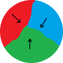
Each $B_{i}$ is called a branch of $\Omega$. Locally, if $x$ is in both $B_{i}$ and $B_{j}$, then $x$ will be translated by both $v_{i}$ and $v_{j}$. Figure 2 represents a piecewise translation of 3 branches on a 2-dimensional disk. These three branches intersect only at their boundaries, which have zero Lebesgue measure. Figure 2 is a simplified model of machine learning. In order for the machine to learn, we need multiple inputs from the environment. Each input is represented by a translation vector. The process of machine learning is modeled by the dynamics of applying the piecewise translation map many times. Therefore, it is natural to define what we get after applying the map over and over again, which we will call the attractor.

Because $\{F^{n}(\Omega)\}_{n=1}^{\infty}$ is a non-increasing sequence of non-empty compact sets, it has a non-empty intersection. Therefore, the attractor is always non-empty and compact. Moreover, the attractor should be invariant under the map $F$. This expected property is a direct consequence of the following lemma.

In some cases, a small change in the translation vectors $v_{0},\,v_{1},\ldots,\,v_{m-1}$ leads to a huge change in the geometry of $A$. In other words, $A$ is not “continuous” in the parameter space. It is convenient to introduce the Hausdorff metric on $\mathcal{X}$ to study the continuity of $A$. Here we denote the $\varepsilon$-neighborhood of a set $X$ with the standard Euclidean metric by $X_{\varepsilon}$. We will show that the orbit of $\Omega$ gets arbitrarily close to the attractor with respect to the Hausdorff metric.

In this section, we are interested in piecewise translation maps of $m=d+1$ branches in $\mathbb{R}^{d}$. We assume that $\text{rank}\{v_{0},v_{1},\ldots,v_{m-1}\}=d$; that is, the vectors in $\mathcal{B}=\{v_{1}-v_{0},v_{2}-v_{0},\ldots,v_{m-1}-v_{0}\}$ form a basis for $\mathbb{R}^{d}$. Let $\mathcal{L}$ be the lattice generated by $\mathcal{B}$, then $\mathbb{T}=\mathbb{R}^{d}/\mathcal{L}$ is a d-dimensional torus. In this case, $v_{0}$ serves as the translation vector in $\mathbb{T}$; i.e. we have the torus rotation map $R:\mathbb{T}\to\mathbb{T},\,R(x+\mathcal{L})=x+v_{0}+\mathcal{L}$. Atom-wise, the action of $F$ is the same as the action of $R$ on $\mathbb{T}$. Globally, it is also true and can be seen through the canonical projection $\pi:\mathbb{R}^{d}\to\mathbb{T},\,\pi(x)=x+\mathcal{L}$.

It was proven that any piecewise translation of an interval with 2 branches is of finite type [18]. However, this does not hold for dimension 2 or higher. Indeed, not all double rotation on a torus is of finite type. In the case where $m=d+1$, there is a space of parameters (translation vectors) where we will get finite type attractors. We assume that the translation vectors $v_{0},\,v_{1},\ldots,v_{m-1}$ are rationally independent, i.e. they are linearly independent in $\mathbb{Q}$-vector space. This is equivalent for the toral map $R$ to be ergodic. In this case, we say that the translation vectors are minimal. With this assumption, the map $F$ is necessarily of finite type. We start with some definitions that will be used in the proof.

In general, it is not true that the attractor is continuous with respect to Hausdorff metric in the parameter space. Even in the case $m=d+1$, we observed that sometimes the two separate pieces of the attractor reglue to each other. One of our concerns has not been proven yet.

However, in the case $m=d+1$, the question of semi-continuity of the attractor is easier to answer. We will show that for a particular family of partitions, finite type attractors are semi-continuous on the translation vectors. Before showing the proof for this, we need a formal definition for semi-continuity of the attractors.

Note that the semi-continuity of the attractor corresponds to the pseudo-Hausdorff metric $d(X,Y)=\sup\{d(x,Y)\mid x\in X\}$. It is clear that

In this section, we discuss a special class of piecewise translations of two branches on a two dimensional torus called double rotations. Double rotations were discussed in [17] and [11]. Synchronization properties of random double rotations on tori were studied in [12]. Here we will show some pictures of double rotations with finite and infinite types.

In Figure 4, the torus is partitioned into two regions - green and blue. We assign a different translation vector to each region. After applying the map, we see that a region from the torus is lost (the red region). In this case, it is the translational image of the green region. Applying the map one more time, we get an additional lost region. Again, this is a translational image of the previous red region. After 500 times, we no longer get any additional lost region. The map is of finite type and its attractor is the blue part in Figure 5. On the other hands, in Figure 6, we do not get the attractor even after 5000 iterates. The map seems to be of infinite type.

Let $\mathcal{V}$ be the space of parameters $\{v_{0},v_{1}\}$ with a fixed partition such that the double rotation map $f_{v_{0},v_{1}}$ is of finite type. By computer simulation, we conjecture that the map is of finite type for almost every parameter. If the map is finite, we also expect the attractor is semi-continuous with respect to Hausdorff distance. This behavior has already been seen in the previous section.

I would like to thank my advisor, Prof. Anton Gorodetski for the patient guidance, encouragement, and advice he provided during my research. I also want to thank UCI UROP for funding me during the summer of 2016 to finish this project.

References

- [1] R. Adler, B. Kitchens, M. Martens, C. Pugh, M. Shub, C. Tresser, Convex dynamics and applications, Ergodic Theory Dynam. Systems, 25 (2005), no. 2, pp. 321–352.
- [2] R. Adler, T. Nowicki, G. Świrszcz, C. Tresser, and S. Winograd, Error diffusion on simplices: Invariant regions, tessellations and acuteness, Preprint, 2012.
- [3] P. Ashwin, J. Deane, X.-C. Fu, Dynamics of a Bandpass Sigma-Delta Modulator as a Piecewise Isometry, Proc. - IEEE Int. Symp. on Circuits and Sys., 3 (2001), pp. 811–814.
- [4] H. Bruin, G. Clack, Inducing and Unique Ergodicity of Double Rotations, Discrete Contin. Dyn. Sys., 32 (2012), pp. 4133–4147.
- [5] M. Boshernitzan, I. Kornfeld, Interval translation mappings, Ergodic Theory Dynam. Systems, 15 (1995), no. 5, pp. 821–832.
- [6] L. Chua, T. Lin, Chaos in digital filters, IEEE Trans. Circuits Syst., vol. CAS-35 (1988), pp. 648–658. 648?58.
- [7] J. Deane, Piecewise Isometries: Applications in Engineering, Meccanica, 41 (2006), pp. 241–252.
- [8] J. Deane, Global attraction in the sigma-delta piecewise isometry, Dynamical Systems 17 (2002), pp. 377–388.
- [9] J. Deane, The buck converter planar piecewise isometry, preprint.
- [10] O. Feely, Nonlinear dynamics of bandpass sigma?elta modulation, Proceedings of NDES, Dublin (1995), pp. 33–36.
- [11] C. Gregory, Double Rotations, Doctoral Thesis, (2013), pp. 20–69.
- [12] A. Gorodetski, V. Kleptsyn, Synchronization properties of random piecewise isometries. Comm. Math. Phys. 345 (2016), no.3, pp. 781–796.
- [13] A. Gorodetski, D. Volk, M. Welling, Some remarks on piecewise translation maps, Print., (2015), pp. 01–16.
- [14] M. Keane, Interval Exchange Transformations, Math. Z. 141 (1975), pp. 25–31.
- [15] H. Masur, Interval Exchange Transformations and Measured Foliations, Ann. of Math., 115 (1982), pp. 169–200.
- [16] H. Suzuki, K. Aihara, T. Okamoto, Complex behaviour of a simple partial discharge model, Europhys. Lett., 66 (2004), pp. 28–34.
- [17] H. Suzuki, S. Ito, K. Aihara, Double rotations. (English summary) Discrete Contin. Dyn. Syst. 13 (2005), no. 2, pp. 515–532.
- [18] D. Volk, Almost every interval translation map of three intervals is finite type. Discrete Contin. Dyn. Syst. 34 (2014), no. 5, pp. 2307–2314.
- [19] D. Volk, Attractors of Piecewise Translation Maps, Preprint., (2017).
- [20] W. Veech, Gauss measures for transformations on the space of interval exchange maps, Ann. of Math., 115 (1982), pp. 201–242.