Observed periodicity related to the four-strand Burau representation

Artin’s braid group $B_{n}$ appears throughout mathematics in many guises, in large part due to its fundamental connection to the motion of sets of particles in the plane. The group $B_{n}$ enjoys many desirable properties, such as finite-presentability and linearity. The latter was established via the faithful Lawrence–Krammer representation of $B_{n}$; however, a long-standing open problem is for which values of $n$ the related Burau representation $\Psi_{n}$ of the braid group is faithful. It is known to be faithful for $n\leq 3$ and not faithful for $n\geq 5$. In this paper, we are concerned with the question of faithfulness when $n=4$, the remaining open case. A non-trivial element in the kernel of $\Psi_{4}$ would give a likely candidate for showing that the Jones polynomial cannot detect the unknot, as noted by Bigelow [2].

The Burau representation’s lack of faithfulness for large $n$ was shown by Moody [6], Long–Paton [5], and Bigelow [1], using related criteria involving combinatorics of pairs of arcs in the $n$-punctured disk $D_{n}$. To each pair of arcs in $D_{n}$ we associate a polynomial called its Burau polynomial. One criterion states that $\Psi_{n}$ is not faithful if and only if there exists a pair of intersecting arcs in an explicit set $\mathcal{A}$ whose Burau polynomial is zero. Ordering arc-pairs by their geometric intersection number, the first main theorem of this paper certifies the faithfulness of the Burau representation $\Psi_{4}$ up to arc-pairs with intersection number 2000.

We prove Theorem A by computer search, identifying then testing a finite yet sufficient collection of arc-pair representatives for each intersection number. We describe the arcs using weighted train tracks, with linear inequalities between the weights being used to ‘steer’ the arcs around the disk $D_{n}$.

Computation of Burau polynomials has been carried out previously. Working with a different collection of arcs in $D_{n}$ referred to as ‘noodles’ and ‘forks’, Bigelow [2] certified the faithfulness of $\Psi_{4}$ up to noodles and forks intersecting 2000 times. Translating this into the language used here, this corresponds to a set of arc-pairs intersecting at most 1000 times. The bound obtained in Theorem A is thus of notable increase. Also, the collection of arcs in [2] and those in Theorem A are of entirely different types. While either collection may be used to certify faithfulness, we are unaware of any way to compare the two. Our approach benefited from decreased computation time, due to several short-cuts we were able to make. These are discussed in detail in Section 4.

One by-product of the proof of Theorem A is the means to list a slew of Burau polynomials. In doing so, a striking periodicity is observed, as we now describe. We define the norm of a Burau polynomial to be the sum of the absolute values of its coefficients. For reasons apparent in the calculation of these polynomials, if seeking the zero polynomial, we need only check arc-pairs with even intersection number. The following theorem records a repetitive structure observed in the minimum norm for such intersection numbers.

The upper bound of 500 was imposed by limits on computation time; this periodicity almost certainly persists longer. Immediately, we observe that if $\Psi_{4}$ is not faithful, there must be some large intersection number at which the periodicity breaks.

We remark that the largest intersection numbers checked in Theorems A and B are of different magnitudes. Both were pushed as high as possible, using hundreds of hours of computation time. However, the former only required testing whether the given polynomials equaled zero, whereas the latter demanded that we form a complete list of Burau polynomials to examine. For a given geometric intersection number, the latter case is more computationally laborious.

A strong relationship is observed between the arcs of minimum norm that appear in Theorem B. Every such arc falls into a family, where within a single family, the train track weights lie in an arithmetic progression and the ordered sets of coefficients of their Burau polynomials are all the same. Attempting to see the behavior of Burau polynomials across all arc-pairs, these ‘minimum norm families’ obscure our view. By grouping all arcs into similar families, we are able to see through the minimum norms obtained for each intersection number and give numerical evidence that suggests $\Psi_{4}$ is faithful. This is discussed further in Section 5.

Outline of paper. In Section 2, we recall the definition of the Burau representation, and state criteria for its faithfulness. Section 3 explains how we use weighted train tracks to describe arcs in the disk $D_{n}$, and how we are able to reduce to only checking arc-pairs of a certain form. Section 4 details the algorithm we constructed, and in Section 5 we report on our observations and numerical evidence.

Acknowledgements. The authors would like to thank Stephen Bigelow, Dan Margalit, and Balázs Strenner for helpful conversations. Part of this work was completed while the first author was in residence at the Mathematical Sciences Research Institute in Berkeley, California, during the Fall 2016 semester.

Let $n\geq 2$. We begin this section by reviewing the definition of the Burau representation

Then we discuss the criterion for faithfulness introduced by Moody and refined by Long–Paton and Bigelow.

Our ultimate aim is to use Theorem 2.1 to certify the faithfulness of $\Psi_{4}$ up to some large number of intersections between the pairs of arcs appearing in the theorem. Given that the existence of a pair $(\alpha,\beta)$ with $\beta$ of type $(3,4)$ and zero Burau polynomial is equivalent to the existence of some pair $(\alpha^{\prime},\beta^{\prime})$ with $\beta^{\prime}$ of type $(0,3)$ and zero Burau polynomial, we limit our search to those of the former type. Thus we will show that, up to some large bound $N$, any arcs $\alpha$ of type $(1,2)$ and $\beta$ of type $(3,4)$ intersecting $N$ times or fewer have non-zero Burau polynomial.

In practice, the techniques we use could be implemented to approach pairs of the latter type. Bigelow carried out a computer search on this latter type using different methods [2]. There, his ‘noodles’ and ‘forks’ are equivalent to arc-pairs of types $(1,2)$ and $(0,3)$: the fork’s tine is an arc of type $(1,2)$, while a noodle $N$ gives rise to an arc of type $(0,i)$, by joining $p_{0}$ to the puncture $p_{i}$ separated from the rest by $N$. We note that passing from a noodle to its arc halves the intersection number with the fork’s tine, resulting in the halving from 2000 to 1000 stated in this paper’s introduction.

Since our focus will be on arc pairs $(\alpha,\beta)$ of types $(1,2)$ and $(3,4)$, we will call any such pair a Burau pair.

Let $\beta$ be an arc belonging to a Burau pair $(\alpha,\beta)$ subject to the reductions of Section 3.3. The boundary of a regular neighborhood of $\beta$ is a loop $\gamma$ supported on $\mu$, and thus we can get a set of weights for $\gamma$. In this section we go the opposite direction, finding necessary and sufficient conditions that a set of weights produces a multicurve $\gamma$, one component of which is a regular neighborhood of an arc $\beta$ belonging to a Burau pair $(\alpha,\beta)$ subject to the reductions of Section 3.3. Not being able to give conditions on the weights to prevent proper multicurves from arising, we instead detect proper multicurves by performing a preliminary computation on a given weight set. Details on this as well as our algorithm are given at the end of this section.

With $\mathbb{N}$ the nonnegative integers, let $(w_{i})_{i=0}^{14}\in\mathbb{N}^{15}$ where $w_{i}$ is the weight of the $i$th rail of $\mu$ as labeled in Figure 5. The switch conditions are expressed by the following equations.

As every weight is freely determined by $w_{0}$, $w_{1}$, $w_{2}$, $w_{3}$, and $w_{14}$, we focus our attention on the tuple $(w_{0},w_{1},w_{2},w_{3},w_{14})$.

Divisibility: The arc $\beta$ starts on rail $6$ and ends on rail $7$, so weights $w_{0}$ and $w_{1}$ are even and weights $w_{2}$ and $w_{3}$ are odd.

Nonnegativity: The weights $w_{8},\ w_{9},\ w_{10},\ w_{11},\ w_{12},$ and $w_{13}$ must be nonnegative.

In the next two groups of conditions, we “steer” the initial and terminal segments as dictated by the reductions in Section 3.3. Consider the track segment seen in Figure 6. Which rail the arc follows is determined by the number of lines $\ell$ that are to the left of the arc as it approaches a switch. Beginning at the switch of $r_{0}$ and $r_{1}$ traveling left, $\ell=w_{0}$. The arc is steered left if and only if $w_{0}<w_{2}$. Assuming this is the case, after passing through the switch of $r_{2}$ and $r_{4}$ we still have $\ell=w_{0}$. On the other hand if the arc is steered right, then after passing through the switch of $r_{3}$ and $r_{4}$ we now have $\ell=w_{0}-w_{2}+w_{4}$. As the notions “initial” and “terminal” are merely a choice of orientation, these remarks equally apply to the terminal segment of the arc.

Initial segment: The arc $\beta$ starts on rail $6$ and then travels on rail $11$, meaning $w_{2}<w_{11}$. After this, $\beta$ intersects the arc $\alpha$ from the top along rail $0$ or $1$, or from the bottom along rail $0$, meaning $w_{9}<w_{2}$ or $w_{1}<w_{2}$. In the case where $\beta$ intersects $\alpha$ from the bottom while traveling along rail $0$, we must enforce that $\beta$ does not then undo this intersection by traveling along rail $8$ and intersecting $\alpha$ from the top, as seen in Figure 7.

Therefore, if $w_{9}<w_{2}$ and $w_{0}<w_{2}-w_{9}+w_{8}$, then $w_{2}-w_{9}+w_{8}<w_{10}$ or $w_{2}+w_{8}-w_{10}<w_{1}$. Using the switch conditions, we translate these into conditions on $w_{0}$, $w_{1}$, $w_{2}$, $w_{3}$, and $w_{14}$.

1. 1.

   $w_{3}<\frac{w_{14}}{2}$

2. 2.

   $w_{1}+\frac{w_{14}}{2}<w_{0}+w_{2}$  or  $w_{1}<w_{2}$

3. 3.

   $w_{0}+w_{2}<w_{1}+\frac{w_{14}}{2}$  or  $w_{0}+w_{2}<w_{14}$  or  $w_{0}+w_{1}+w_{2}<3\frac{w_{14}}{2}$  or  $w_{1}+w_{2}<w_{14}$

Terminal segment: The terminal segment of $\beta$ is seen in Figure 8.

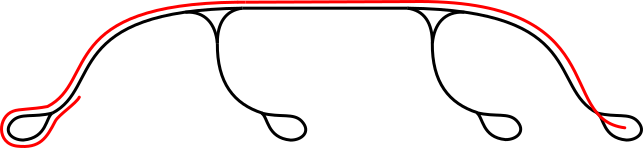
This translates into the conditions $w_{12}<w_{3}$, $w_{9}<w_{3}-w_{12}+w_{11}$, and $w_{0}<w_{3}-w_{12}+w_{11}-w_{9}+w_{8}$. Immediately prior to taking this path, the arc cannot travel on rail $1$ intersecting $\alpha$ from below. This gives the fourth condition

Again using the switch conditions, we express these in terms of $w_{0}$, $w_{1}$, $w_{2}$, $w_{3}$, and $w_{14}$.

In order to prove that the conditions we have given are sufficient, we will use the following lemma.

There are two ways we can prevent certain proper multicurves from arising. The first is to insist that $\gcd(w_{0},w_{1},w_{2},w_{3})=1$, as otherwise all weights will share a non-trivial common factor and give rise to multiple copies of a single, simple closed curve. The second is to insist that some weight is zero, as otherwise the resulting multicurve will have a loop encompassing the entire train track and thus be a proper multicurve. The paths of the initial and terminal segments of the corresponding arc imply that all weights except for $w_{1}$, $w_{8}$, $w_{9}$, and $w_{12}$ are non-zero. Since $w_{1}$ being zero implies that $w_{8}$ and $w_{9}$ are zero, we have three cases.

1. 1.

   $w_{8}=0$, meaning $\frac{w_{14}}{2}=w_{0}+w_{1}$

2. 2.

   $w_{9}=0$, meaning $\frac{w_{14}}{2}=w_{0}-w_{1}$

3. 3.

   $w_{12}=0$, meaning $\frac{w_{14}}{2}=w_{2}+w_{3}$

All three cases can occur simultaneously. In each case, many of the above conditions become satisfied or simplified. The conditions D1-D4 remain in all cases, and the other conditions become the following.

Case I.

N1. $w_{0}+w_{1}\leq w_{2}+w_{3}$   I2. $w_{1}<w_{2}$   T1. $w_{2}<w_{0}+w_{1}$   T3. $w_{3}<w_{0}$

When traveling on rail $14$ either moving left or right, the conditions on the initial and terminal segments imply that there are only a finite number of possible paths one may take before returning to rail $14$. These paths are enumerated in Figure 11.

Let $\ell$ denote the number of lines to the left of the arc as it travels on rail 14. Which of the enumerated paths is taken, along with the direction this path is traversed, is determined by comparing $\ell$ to the train track weights. When traveling to the left, the path and direction are determined by the position of the first number that $\ell$ is smaller than in the following list.

Likewise when traveling to the right, the path and direction are determined by the position of the first number that $\ell$ is smaller than in the following list.

Note that for a given set of weights, it may be that either of the lists are not ascending. This can occur when an arc never takes one of the paths enumerated in Figure 9 and Figure 10.

To compute the resulting Burau polynomial, our algorithm begins with $\ell=w_{2}$ and the Burau polynomial being $0$. We then alternate traveling left and right on rail $14$. Each time a path is taken, we update $\ell$ and the Burau polynomial accordingly. We end the computation when the arc reaches rail $7$ with $\ell=w_{3}$. While traveling right on rail 14, this is precisely when we have either $\ell=w_{3}$ and $\ell<\ w_{13}$, or $\ell$ is greater than all the numbers in the list above and $\ell=3w_{3}+w_{14}$. Along with being computationally efficient, this allows us to concisely describe the path of an arc. Each time we return to rail 14, using the appropriate list we record the position of the first number that $\ell$ is smaller than, $1-8$ and $1-6$ respectively. We call the resulting list the record of the arc $\beta$.

We achieve a significant speedup by doing a preliminary run on each arc, recording the number of positive and negative crossings. We discard the weight set if a proper multicurve is ever detected, which by Corollary 4.3 is the case if and only if the number of crossings is less than $\frac{w_{0}}{2}+\frac{w_{1}}{2}-\min(w_{1},w_{8})$. During the preliminary run, we also use a static array of size $2^{m}$ to compute the Burau polynomial where the powers of $t$ are treated modulo $2^{m}$. On our system, $m=7$ appears to be optimal. When we are solely searching for the zero polynomial, we short-circuit the computation if the array is not all zero.

For an arc $\beta$ belonging to a Burau pair $(\alpha,\beta)$, we denote by $\vec{w}_{\beta}$ the corresponding weights on $\mu$, $c(\beta)$ the number of crossings with $\alpha$, and $p_{\beta}(t)$ the resulting Burau polynomial. For each $k\in\mathbb{N}$, the arcs of level $2k$ are $\left\{\beta:c(\beta)=2k\right\}$. Our implementation has resulted in the following theorem.

Finding no arc-pair asserting the unfaithfulness of $\Psi_{4}$, we proceed with a more qualitative analysis. Define the minimum norm and multiplicity of a level $2k$ to be

The initial levels have erratic behavior.

However after this appears remarkable periodicity.

The periodic behavior in Theorem 5.2 is a result of the arcs falling into into families.

Our computations have shown that all arcs $\beta$ with $c(\beta)\in[44,500]$ and $|p_{\beta}(t)|=\minnorm(c(\beta))$ fall into $6+18+18$ families whose weights are in an arithmetic progression and whose ordered set of coefficients of the resulting Burau polynomials are constant.

There are a variety of ways that these families arise, the simplest is as follows. Let $\beta$ be an arc, $p$ a point on $\beta$, and $\gamma$ a loop that only intersects itself or $\beta$ at $p$. Then with some perturbations one can construct new arcs by repeatedly inserting $\gamma$ into $\beta$. An example of this form is seen in Figure 12. Note that doing this does not guarantee that the resulting Burau polynomial norms will all be equal, nor that the resulting polynomials themselves will all be of a similar form. More complicated patterns also give rise to families, as seen in Figure 13 where there are two loops inserted in an interleaving fashion.

The families in Figure 12 and Figure 13 are not one of the $6+18+18$ families in Theorem 5.2. Indeed, the families in Theorem 5.2 would be quite difficult to draw. In order to see their behavior, we can look at records of the arcs. Consider Example 5.3 above, but now with $m=\frac{2k-6}{6}$ where $2k\equiv 0\ (\text{mod }6)$ and $2k\in[6,500]$. The records of the first three members of this family are as follows.

The $m$th member is achieved by inserting the arc with record $4,1,2,4,2,4,2,5,3,5,3,5$ $m$-times. Another family of arcs that gives rise to the minimum norms of Theorem 5.2 has the following records.

Here the arcs $3,5,3,5,3$ and $6,5,4,2,4,2,4$ are interleaved. In each of these examples, the initial members of the family do not give rise to Burau polynomials with the same ordered set of coefficients. It is only the later members that have this behavior.

Grouping the arcs into families, the periodicity observed in Theorem 5.2 is recast into an observation about $6+18+18$ families. These families always being of minimal norm block us from seeing the behavior of other arcs. In order to see through this obstruction, we group all arcs into “tightly-knit” families and study the minimum norm where we ignore any noninitial member of such a family.

Let $\mathcal{F}=\left\{\beta_{i}\right\}_{i=0}^{\infty}$ be a collection of arcs and set $\vec{d}=\vec{w}_{\beta_{1}}-\vec{w}_{\beta_{0}}$. We say that $\mathcal{F}$ is a tightly-knit family if for all $i\in\mathbb{N}$, $\vec{w}_{\beta_{i}}=\vec{w}_{\beta_{0}}+i\cdot\vec{d}$ and $p_{\beta_{i}}(t)$ has the same ordered set of coefficients as $p_{\beta_{0}}(t)$. We call this the tightly-knit family generated by $\beta_{0}$ and $\beta_{1}$. For such a family we define $c(\mathcal{F})=c(\beta_{0})$.

Note that any given arc can lie in many tightly-knit families. Let $\beta$ and $\beta^{\prime}$ be two distinct arcs with the entries of $\vec{w}_{\beta^{\prime}}-\vec{w}_{\beta}$ all nonnegative. Then $\beta$ and $\beta^{\prime}$ lie in a tightly-knit family if and only if $\beta_{0}=\beta$ and $\beta_{1}=\beta^{\prime}$ themselves generate a tightly-knit family. To check that $\beta$ and $\beta^{\prime}$ belong to the same family in computations, we must restrict ourselves to testing the first $m\in\mathbb{N}$ members generated by $\beta$ and $\beta^{\prime}$. In the results below, we first used $m=100$ and then $m=1000$. In each case, the results remain unchanged.

For $k\in\mathbb{N}$ we define

Note that there exists a positive $k\in\mathbb{N}$ such that $\min(2k)=0$ if and only if $\Psi_{4}$ is unfaithful. We emphasize that in computing $\min(2k)$ for $2k\in[2,200]$, seen in Figure 14(a), we only test the first $100$, and then $1000$, members to determine if a collection forms a tightly-knit family.

By weakening the definition of a tightly-knit family while maintaining the property that there exists a positive $k\in\mathbb{N}$ such that $\min(2k)=0$ if and only if $\Psi_{4}$ is unfaithful, we can seek different ways to group the arcs into families, studying their behavior as the number of intersections increase. With this in mind, we say that $\mathcal{F}=\left\{\beta_{i}\right\}_{i=0}^{\infty}$ is a loosely-knit family if for all $i\in\mathbb{N}$, $\vec{w}_{\beta_{i}}=\vec{w}_{\beta_{0}}+i\cdot(\vec{w}_{\beta_{1}}-\vec{w}_{\beta_{0}})$ and $|p_{\beta_{i}}(t)|\geq|p_{\beta_{0}}(t)|$ for all $i\in\mathbb{N}$. The result of computing $\min(2k)$ for $2k\in[2,200]$ using loosely-knit families is seen in Figure 14, again with the computational limitations as mentioned above.

We interpret the upward trend of these graphs as being suggestive that $\Psi_{4}$ is faithful.

References

- [1] Stephen Bigelow. The Burau representation is not faithful for . Geom. Topol., 3:397–404, 1999.
- [2] Stephen Bigelow. Does the Jones polynomial detect the unknot? J. Knot Theory Ramifications, 11(4):493–505, 2002. Knots 2000 Korea, Vol. 2 (Yongpyong).
- [3] Joan S. Birman. Braids, links, and mapping class groups. Princeton University Press, Princeton, N.J.; University of Tokyo Press, Tokyo, 1974. Annals of Mathematics Studies, No. 82.
- [4] Benson Farb and Dan Margalit. A primer on mapping class groups, volume 49 of Princeton Mathematical Series. Princeton University Press, Princeton, NJ, 2012.
- [5] D. D. Long and M. Paton. The Burau representation is not faithful for . Topology, 32(2):439–447, 1993.
- [6] John Atwell Moody. The Burau representation of the braid group is unfaithful for large . Bull. Amer. Math. Soc. (N.S.), 25(2):379–384, 1991.