跳到论文正文
W Papers独立论文阅读器 arXiv:1610.04454 论文正文 计算阅读时间 · 0%
引用这篇论文根据当前论文元数据生成,正式投稿前建议核对。


License: arXiv.org perpetual non-exclusive license
arXiv:1610.04454v3 [cs.GT] 14 Feb 2018

A Budget Feasible Mechanism for Hiring Doctors in E-Healthcare

Vikash Kumar Singh Affiliation: Dept. of Computer Science and Engineering
National Institute of Technology
Durgapur 713209, India
vikas.1688@gmail.com
   Sajal Mukhopadhyay Affiliation: Dept. of Computer Science and Engineering
National Institute of Technology
Durgapur 713209, India
sajal@cse.nitdgp.ac.in
   Fatos Xhafa Affiliation: Dept. of Computer Science
Universitat Polite`\grave{e}cnica de Catalunya
Barcelona 08034, Spain
fatos@cs.upc.edu
   Aniruddh Sharma Affiliation: Dept. of Computer Science and Engineering
National Institute of Technology
Durgapur 713209, India
aniruddhsharma189@gmail.com
Abstract

Throughout the past decade, there has been an extensive research on scheduling the hospital resources such as the operation theatre(s) (OTs) and the experts (such as nurses, doctors etc.) inside the hospitals. With the technological growth, mainly advancement in communication media (such as smart phones, video conferencing, smart watches etc.) one may think of taking the expertise by the doctors (distributed around the globe) from outside the in-house hospitals. Earlier this interesting situation of hiring doctors from outside the hospitals has been studied from monetary (with patient having infinite budget) and non-monetary perspectives in strategic setting. In this paper, the more realistic situation is studied in terms of hiring the doctors from outside the hospital when a patient is constrained by budget. Our proposed mechanisms follow the two pass mechanism design framework each consisting of allocation rule and payment rule. Through simulations, we evaluate the performance and validate our proposed mechanisms.

Index Terms: 
e-healthcare; hiring doctors; budget; truthful

I Introduction

Substantial literatures are available to schedule resources inside the hospitals in healthcare system [1][2][3][4]. However, how to hire (to schedule) resources (expert consultants (ECs) etc.) along with their pricing schemes from outside the hospitals are mostly unaddressed [5][6][7][8]. It is observed that, with the prodigious growth of the communication media (say video conferencing, Internet, smart phones etc.), it may be an usual phenomena to have the consultancies by the experts (especially doctors) from outside the hospital(s). It is to be noted that the doctors can provide consultancies by being present at the consultancy spot (where the patient is admitted) particularly virtually (using video conferencing, Internet, smart phones etc.) etc. making them pervasive. In our future references ECs and doctors will be used interchangeably. In this paper, an attempt is made to hire expert consultants from outside the hospital when a patient is budget limited. The detailing of the hiring concept in this paper is shown in Figure 1. In our model, the hiring concept is shown as a two fold process. In the first fold, the accumulated hospital’s budget can be utilized to detect the leaders in the social graph (representing ECs professional connections) to inform about the hiring concept to the substantial number of doctors.

Refer to caption
Fig. 1: System model

In the second fold, the subset of doctors will be selected from the set consisting of doctors as leaders and the informed doctors for the consultancy process, such that the total payment made to the doctors is within patient’s budget.
The remainder of the paper is structured as follows. Section II elucidates the related works. Section III describes our proposed model. The proposed mechanisms are illustrated in section IV. The analysis of the proposed mechanisms are illustrated in section V. In section VI experiments and results are shown. Finally, conclusions are drawn in Section VII.

II Related prior work

In past the handful of works have been done, focusing on scheduling inside the hospitals (or internal scheduling) in terms of operation theatres (OTs) scheduling [9][1][2][10] and internal staffs (such as nurses [3][11], physicians [12][4] etc.) scheduling. In [13][10] the works have been done for allocating OTs on time to increase OTs efficiency. In our future references, hospital(s), medical unit(s), organization(s) will be used interchangeably. As with the enhancement in the technologies, mainly communication media (say video conferencing, Internet, smart phones etc.), it may be an usual phenomena to think of the scheduling of medical staffs (mainly doctors) outside the in-house hospital [5][6][14]. In [5] a doctor is providing the expertise through video conferencing to a patient admitted to other hospital with prior contact. In [15] the context of the patient (such as age, sex, medical report etc.) is utilized to take the expertise of the doctors from outside the admitted hospitals in non-strategic setting. In [6] the strategic case is considered and is solved using mechanism design with money and in [7][8] mechanism design without money is utilized. Despite some progress in the scenario of hiring ECs from outside the hospital(s), the patients with budget constraints case has been largely overlooked. In this paper, the problem of hiring doctors from outside the hospital is studied in this setting.

III System model

III-A Notation and Preliminaries

In this section, we formalize the doctors hiring problem where the multiple doctors are hired from outside of the hospital, for a patient having budget 𝓑′\boldsymbol{\mathcal{B}^{\prime}}. The patient’s budget 𝓑′\boldsymbol{\mathcal{B}^{\prime}} is a public information. The hospital to which a patient is admitted is having an accumulated, publicly known budget 𝓑\boldsymbol{\mathcal{B}}, which will be utilized to inform about the hiring concept to the substantial number of ECs. The set of ECs is given as 𝒮={s1,s2,…,sm}\mathcal{S}=\{s_{1},s_{2},\ldots,s_{m}\}; where each EC si∈𝒮s_{i}\in\mathcal{S} is assumed to be professionally connected with some χi⊆𝒮\chi_{i}\subseteq\mathcal{S}∖\setminus{si}\{s_{i}\}. The professional connections are given by a social graph 𝒢⁡(𝒱,ℰ)\mathcal{\mathcal{G}(\mathcal{V},\mathcal{E})}, where 𝒱\mathcal{V} is the set of nodes representing ECs and ℰ\mathcal{E} is the set of edges representing their professional connections in the social graph. Each sis_{i} is associated with a hospital ℏi∈𝓗\hbar_{i}\in\boldsymbol{\mathcal{H}}. Our model consists of two fold process. In the first fold, there is a social graph that is represented as 𝒢⁡(𝒱,ℰ)\mathcal{\mathcal{G}(\mathcal{V},\mathcal{E})} and publicly known expert consultant activation function given as 𝓘:2𝒮→𝓡≥𝟎\boldsymbol{\mathcal{I}}:2^{\mathcal{S}}\rightarrow\boldsymbol{\mathcal{R}_{\geq 0}}. Given the subset Γ⊆𝒮\varGamma\subseteq\mathcal{S} the value ℐ⁡(Γ)\mathcal{I}(\varGamma) represents the expected number of doctors that are made aware about the hiring concept i.e.i.e. I⁡(Γ)=|⋃i∈Γ​χi|I(\varGamma)=|\underset{i\in\varGamma}{\bigcup}\chi_{i}|. Each node in the graph represents a doctor sis_{i} that has a private cost (aka bid) cic_{i} of being an initial adapter or the cost for spreading awareness about the hiring concept to other doctors. The cost vector of all the mm doctors is given as: 𝓒={c1,c2,…,cm}\boldsymbol{\mathcal{C}}=\{c_{1},c_{2},\ldots,c_{m}\}. It is to be noted that, the ECs are rational and strategic in nature. It means that, the ECs can gain by misreporting their private cost. As the ECs are strategic; so each si∈𝒮s_{i}\in\mathcal{S} may report their cost for being an initial adapter as ci′c^{\prime}_{i} instead of cic_{i} in order to gain; where ci′≠cic^{\prime}_{i}\neq c_{i}. The payment vector for the set Γ\varGamma is given as 𝓟Γ\boldsymbol{\mathcal{P}}_{\varGamma} = {𝓟Γ1,𝓟Γ2,…,𝓟Γk}\{\boldsymbol{\mathcal{P}}_{\varGamma_{1}},\boldsymbol{\mathcal{P}}_{\varGamma_{2}},\ldots,\boldsymbol{\mathcal{P}}_{\varGamma_{k}}\}; where 𝓟Γi\boldsymbol{\mathcal{P}}_{\varGamma_{i}} is the payment of si∈Γs_{i}\in\varGamma. The objective of the first fold is to maximize the expert consultant activation function while the total payment is at most hospital’s budget 𝓑\boldsymbol{\mathcal{B}}. In the second fold, we have a set of doctors consisting of doctors acted as leaders in the first fold and the aware doctors given as 𝒮^={s1,s2,…,si−1,si,…,sn}\hat{\mathcal{S}}=\{s_{1},s_{2},\ldots,s_{i-1},s_{i},\ldots,s_{n}\} such that n≤mn\leq m. The quality vector of all the mm ECs is given as 𝓠={𝒬1,𝒬2,…,𝒬m}\boldsymbol{\mathcal{Q}}=\{\mathcal{Q}_{1},\mathcal{Q}_{2},\ldots,\mathcal{Q}_{m}\}, where 𝒬i∈𝓠\mathcal{Q}_{i}\in\boldsymbol{\mathcal{Q}} is the quality of it​hi^{th} doctor. In general, the quality 𝒬i\mathcal{Q}_{i} of a doctor sis_{i} can be estimated using various parameters calculated later in the section. The publicly known quality function is given as 𝓓:2𝒮^→𝓡≥𝟎\boldsymbol{\mathcal{D}}:2^{\hat{\mathcal{S}}}\rightarrow\boldsymbol{\mathcal{R}_{\geq 0}}. Given a subset Υ⊆𝒮^\varUpsilon\subseteq\hat{\mathcal{S}}, the value 𝓓⁡(Υ)\boldsymbol{\mathcal{D}}(\varUpsilon) denotes the sum of the qualities of all the doctors in Υ\varUpsilon i.e.i.e. 𝓓⁡(Υ)=∑i∈Υ𝒬i\boldsymbol{\mathcal{D}}(\varUpsilon)=\sum_{i\in\varUpsilon}\mathcal{Q}_{i}. For this fold, each doctor si∈𝒮^s_{i}\in\hat{\mathcal{S}} will bid afresh their cost (private) for providing consultancy to the patient and is given as c¯i\bar{c}_{i}. The cost vector of all the n doctors is given as: 𝓒¯={c¯1,c¯2,…,c¯n}\boldsymbol{\mathcal{\bar{C}}}=\{\bar{c}_{1},\bar{c}_{2},\ldots,\bar{c}_{n}\}. The strategic behaviour of the doctors is continued in this fold also; so each si∈𝒮^s_{i}\in\hat{\mathcal{S}} may report their cost of consultancy as c¯i′\bar{c}^{\prime}_{i} instead of c¯i\bar{c}_{i} in order to gain; where c¯i′≠c¯i\bar{c}^{\prime}_{i}\neq\bar{c}_{i}. Our objective is to determine the subset Υ∈{ξ|∑i∈ξc¯i≤𝓑′}\varUpsilon\in\{\xi|\sum_{i\in\xi}\bar{c}_{i}\leq\boldsymbol{\mathcal{B}}^{\prime}\} for which 𝓓⁡(Υ)\boldsymbol{\mathcal{D}}(\varUpsilon) is maximized and the total payment should not exceed the patient’s budget 𝓑′\boldsymbol{\mathcal{B}}^{\prime}. The payment vector of the set Υ\varUpsilon is given as 𝓟^\hat{\boldsymbol{\mathcal{P}}} = {𝓟^1\{\hat{\boldsymbol{\mathcal{P}}}_{1}, 𝓟^2\hat{\boldsymbol{\mathcal{P}}}_{2}, …, 𝓟^r}\hat{\boldsymbol{\mathcal{P}}}_{r}\}.

III-B Quality determination

The parameters that determine the quality of each doctor sis_{i} are: (1) qualification of sis_{i} given as qiq_{i} (2) success rate of sis_{i} given as s​risr_{i} (3) experience of sis_{i} given as eie_{i} (4) hospital to which sis_{i} belong given as ℏi\hbar_{i}. So, the quality of doctor sis_{i} is given as: 𝒬i=(w1⋅qi+w2⋅s​ri+w3⋅ei+w4⋅ℏi)\mathcal{Q}_{i}=\left(w_{1}\cdot q_{i}+w_{2}\cdot sr_{i}+w_{3}\cdot e_{i}+w_{4}\cdot\hbar_{i}\right); where, wi∈[0,1]w_{i}\in[0,1] such that ∑iwi=1\sum_{i}w_{i}=1. The weighted sum of the some of the parameters considered in our case will result in the quality of the doctors.

III-C Budget distribution and utilization

In our scenario, each fold is utilizing the budget from two independent sources. Firstly, talking about the hospital’s budget it can be thought of as 1) the accumulated fund from the previously admitted patients say adding 5-6% of the total fees of each patients to the hospital fund. 2) Donation to the hospital by high profile persons or communities. Next, the source of the budget utilized in the second phase is the patient itself.

Definition 1 (Marginal Contribution [16]).

The marginal contribution of an EC si∈𝒮s_{i}\in\mathcal{S} is the number of ECs informed about the hiring concept by the EC sis_{i} given the set of i−1i-1 ECs i.e.i.e. Γi−1\varGamma_{i-1} already selected as the leaders. Mathematically, the marginal contribution of it​hi^{th} EC given Γi−1\varGamma_{i-1} is defined as: 𝓜𝓒i​(Γi−1)=𝓘⁡(Γi−1∪{si})−𝓘⁡(Γi−1)\boldsymbol{\mathcal{M}}_{\boldsymbol{\mathcal{C}}_{i}}(\varGamma_{i-1})=\boldsymbol{\mathcal{I}}(\varGamma_{i-1}\cup\{s_{i}\})-\boldsymbol{\mathcal{I}}(\varGamma_{i-1})

Definition 2 (Quality Contribution [17]).

The quality contribution of an EC si∈𝒮s_{i}\in\mathcal{S} given a subset Υi−1\varUpsilon_{i-1} of ECs already been selected is given as: 𝓓i​(Υi−1)=𝓓⁡(Υi−1∪{si})−𝓓⁡(Υi−1)\boldsymbol{\mathcal{D}}_{i}(\varUpsilon_{i-1})=\boldsymbol{\mathcal{D}}(\varUpsilon_{i-1}\cup\{s_{i}\})-\boldsymbol{\mathcal{D}}(\varUpsilon_{i-1}) where 𝓓⁡(Υi)\boldsymbol{\mathcal{D}}(\varUpsilon_{i}) denotes the sum of the qualities of all the doctors in Υi\varUpsilon_{i} i.e.i.e. 𝓓⁡(Υi)=∑i𝒬i\boldsymbol{\mathcal{D}}(\varUpsilon_{i})=\sum_{i}\mathcal{Q}_{i} given Υi={1,…,i}\varUpsilon_{i}=\{1,\ldots,i\} and 𝓓⁡(Υ0)=0\boldsymbol{\mathcal{D}}(\varUpsilon_{0})=0 as Υ0=ϕ\varUpsilon_{0}=\phi.

IV Proposed mechanisms

In this section, we present proposed mechanisms: Non-truthful budget constraint (NoTBC) mechanism motivated by [18] and Truthful budget constraint (TBC) mechanism motivated by [16][17].

IV-A NoTBC mechanism

It is a two pass mechanism consisting of Non-truthful budget constraint leader identification (NoTBC-LI) mechanism and Non-truthful budget constraint doctor selection (NoTBC-DS) mechanism.

IV-A1 NoTBC-LI mechanism

In each iteration of while loop, a doctor with maximum marginal contribution per cost among the available doctors is considered and is selected only if its cost for being an initial adapter is less than the hospital’s available budget. The payment of each doctors as a leader is their revealed cost.

Algorithm 1 NoTBC-LI mechanism (𝒢\mathcal{G}, 𝒮\mathcal{S}, 𝓑\boldsymbol{\mathcal{B}}, 𝓒\boldsymbol{\mathcal{C}})
1: 𝒮^\hat{\mathcal{S}} ←\leftarrow ϕ\phi, 𝓟Γ←ϕ\boldsymbol{\mathcal{P}}_{\varGamma}\leftarrow\phi
2: 𝒮¯\bar{\mathcal{S}} ←\leftarrow ϕ\phi ⊳\triangleright Set containing all the informed doctors.
3: while 𝒮≠ϕ\mathcal{S}\neq\phi do
4:   sis_{i} ←\leftarrow a​r​g​m​a​xj∈𝒮argmax_{j\in\mathcal{S}} [𝓜𝓒j​(Γj−1)cj]\left[\frac{\boldsymbol{\mathcal{M}}_{\boldsymbol{\mathcal{C}}_{j}}(\varGamma_{j-1})}{c_{j}}\right]
5:   if ci≤𝓑c_{i}\leq\boldsymbol{\mathcal{B}} then
6:    Γ\varGamma ←\leftarrow Γ\varGamma ∪\cup {si}\{s_{i}\}; 𝒮¯\bar{\mathcal{S}} ←\leftarrow 𝒮¯\bar{\mathcal{S}} ∪\cup {χi}\{\chi_{i}\}; 𝓑←𝓑−ci\boldsymbol{\mathcal{B}}\leftarrow\boldsymbol{\mathcal{B}}-c_{i}
7:   end if
8:   𝒮←𝒮∖{si}\mathcal{S}\leftarrow\mathcal{S}\setminus\{s_{i}\}
9: end while
10: 𝒮^=Γ∪𝒮¯\hat{\mathcal{S}}=\varGamma\cup\bar{\mathcal{S}}
11: for e​a​c​heach sis_{i} ∈\in Γ\varGamma do
12:   𝓟Γi←ci\boldsymbol{\mathcal{P}}_{\varGamma_{i}}\leftarrow c_{i}; 𝓟Γ←𝓟Γ∪{𝓟Γi}\boldsymbol{\mathcal{P}}_{\varGamma}\leftarrow\boldsymbol{\mathcal{P}}_{\varGamma}\cup\{\boldsymbol{\mathcal{P}}_{\varGamma_{i}}\}
13: end for
14: return 𝒮^\hat{\mathcal{S}}, 𝓟Γ\boldsymbol{\mathcal{P}}_{\varGamma}

IV-A2 NoTBC-DS mechanism

In each iteration of while loop, a doctor with maximum quality contribution per cost among the selected doctors by NoTBC-LI mechanism is considered and is hired only if its cost for the consultancy is less than the patient’s available budget. The payment of each hired doctors is their revealed cost of consultancy.

Lemma 1.

The NoTBC mechanism is computationally efficient.

Proof.

In NoTBC-LI, for m iteration of while loop we have O⁡(m2)O(m^{2}). Thus, the running time of NoTBC-LI is O⁡(m2)O(m^{2}). In NoTBC-DS, for mm iteration (in worst case) of while loop we have O⁡(m2)O(m^{2}). Thus, the running time of NoTBC-DS is O⁡(m2)O(m^{2}). In both the cases, the payment determination will be linear in m. Thus, the computational complexity of NoTBC is given as O⁡(m2)O(m^{2}). ∎

Algorithm 2 NoTBC-DS mechanism (𝒮^\hat{\mathcal{S}}, 𝓑′\boldsymbol{\mathcal{B}}^{\prime}, 𝓒¯\boldsymbol{\mathcal{\bar{C}}})
1: Υ\varUpsilon ←\leftarrow ϕ\phi, 𝓟^←ϕ\hat{\boldsymbol{\mathcal{P}}}\leftarrow\phi
2: while 𝒮^≠ϕ\hat{\mathcal{S}}\neq\phi do
3:   sis_{i} ←\leftarrow a​r​g​m​a​xj∈𝒮^argmax_{j\in\hat{\mathcal{S}}} 𝓓j​(Υj−1)c¯j\frac{\boldsymbol{\mathcal{D}}_{j}(\varUpsilon_{j-1})}{\bar{c}_{j}}
4:   if c¯i≤𝓑′\bar{c}_{i}\leq\boldsymbol{\mathcal{B}^{\prime}} then
5:    Υ\varUpsilon ←\leftarrow Υ\varUpsilon ∪\cup {si}\{s_{i}\}; 𝓑′←𝓑′−c¯i\boldsymbol{\mathcal{B}^{\prime}}\leftarrow\boldsymbol{\mathcal{B}^{\prime}}-\bar{c}_{i}
6:   end if
7:   𝒮^←𝒮^∖{si}\hat{\mathcal{S}}\leftarrow\hat{\mathcal{S}}\setminus\{s_{i}\}
8: end while
9: for e​a​c​heach sis_{i} ∈\in Υ\varUpsilon do
10:   𝓟^i←c¯i\hat{\boldsymbol{\mathcal{P}}}_{i}\leftarrow\bar{c}_{i}; 𝓟^←𝓟^∪{𝓟^i}\hat{\boldsymbol{\mathcal{P}}}\leftarrow\hat{\boldsymbol{\mathcal{P}}}\cup\{\hat{\boldsymbol{\mathcal{P}}}_{i}\}
11: end for
12: return Υ\varUpsilon, 𝓟^\hat{\boldsymbol{\mathcal{P}}}
Lemma 2.

The NoTBC mechanism is individually rational.

Proof.

From line 11 of Algorithm 1, we can see 𝓟Γi\boldsymbol{\mathcal{P}}_{\varGamma_{i}} = cic_{i} for each si∈Γs_{i}\in\varGamma. Line 9 in Algorithm 2 shows that 𝓟^i\hat{\boldsymbol{\mathcal{P}}}_{i} = c¯i\bar{c}_{i}. Therefore, we have payment for any winner is its cost. Hence, NoTBC mechanism is individually rational. ∎

Lemma 3.

The NoTBC mechanism is budget feasible.

Proof.

As it is clear that a doctor is included in the winning set only when the given condition in line 4 of Algorithm 1 and line 3 of Algorithm 2 is satisfied. As the payment in case of NoTBC is equal to the cost; the total payment will be at most the budget. Hence, NoTBC mechanism is budget feasible. ∎

IV-B TBC mechanism

It is a two pass mechanism consisting of Truthful budget constraint leader identification (TBC-LI) and Truthful budget constraint doctor selection (TBC-DS) mechanisms.

IV-B1 TBC-LI mechanism

For first fold of hiring problem, we propose a TBC-LI mechanism motivated by [16][17].

Allocation rule

In this, a doctor with maximum marginal contribution per cost among the available doctors

Algorithm 3 TBC-LI allocation mechanism (𝒢\mathcal{G}, 𝒮\mathcal{S}, 𝓑\boldsymbol{\mathcal{B}}, 𝓒\boldsymbol{\mathcal{C}})
1: Γ←ϕ\varGamma\leftarrow\phi, 𝒮^\hat{\mathcal{S}} ←\leftarrow ϕ\phi
2: 𝒮¯←ϕ\bar{\mathcal{S}}\leftarrow\phi; sis_{i} ←\leftarrow a​r​g​m​a​xj∈𝒮argmax_{j\in\mathcal{S}} [𝓜𝓒j​(Γj−1)cj]\left[\frac{\boldsymbol{\mathcal{M}}_{\boldsymbol{\mathcal{C}}_{j}}(\varGamma_{j-1})}{c_{j}}\right]
3: while cic_{i} ≤\leq 𝓑2\frac{\boldsymbol{\mathcal{B}}}{2} (𝓜𝓒i​(Γi−1)𝓜𝓒i​(Γi−1)+𝓘⁡(Γi−1))\left(\frac{\boldsymbol{\mathcal{M}}_{\boldsymbol{\mathcal{C}}_{i}}(\varGamma_{i-1})}{\boldsymbol{\mathcal{M}}_{\boldsymbol{\mathcal{C}}_{i}}(\varGamma_{i-1})+\boldsymbol{\mathcal{I}}(\varGamma_{i-1})}\right) do
4:   Γ\varGamma ←\leftarrow Γ\varGamma ∪\cup {si}\{s_{i}\}; 𝒮¯\bar{\mathcal{S}} ←\leftarrow 𝒮¯\bar{\mathcal{S}} ∪\cup {χi}\{\chi_{i}\}
5:   sis_{i} ←\leftarrow a​r​g​m​a​xj∈𝒮∖Γ​[𝓜𝓒j​(Γj−1)cj]argmax_{j\in\mathcal{S}\setminus\varGamma}\left[\frac{\boldsymbol{\mathcal{M}}_{\boldsymbol{\mathcal{C}}_{j}}(\varGamma_{j-1})}{c_{j}}\right]
6: end while
7: 𝒮^=Γ∪𝒮¯\hat{\mathcal{S}}=\varGamma\cup\bar{\mathcal{S}}
8: return Γ\varGamma and 𝒮^\hat{\mathcal{S}}

is considered. But the doctor is selected as the leader only when the ratio between their cost as the initial adapter and budget is less than or equal to half of the ratio between their marginal contribution and the value of the selected subset.
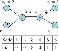
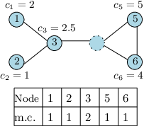
Example 1(a): Figure 2(a) show the initial configuration of the social graph along with cost distribution, and marginal contribution (m.c.). The quality vector of the nodes is given as: 𝓠={5,1,3,5,4,5}\boldsymbol{\mathcal{Q}}=\{5,~1,~3,~5,~4,~5\}. Higher the value, higher will be the quality. For understanding purpose we are taking the quality of the doctors as an integer value but in general it may not be the case. It is to be noted that the unit of cost and budget is taken as $. We have considered hospital’s budget to be 10. Using line 1 of the Algorithm 3 the node 4 is considered.

Refer to caption
(a) Initial configuration
Refer to caption
(b) Intermediate configuration
Fig. 2: Detailed functioning of Algorithm 3

The condition 2≤5⋅(33+0)2\leq 5\cdotp(\frac{3}{3+0}) for node 4 is satisfied. So, Γ={4}\varGamma=\{4\} and 𝒮¯={3,5,6}\bar{\mathcal{S}}=\{3,~5,~6\}. Next, node 3 will be considered and 2.5≤5⋅(33+3)2.5\leq 5\cdotp(\frac{3}{3+3}) for node 3 is satisfied. So, Γ={4,3}\varGamma=\{4,~3\} and 𝒮¯={3,5,6,1,2,4}\bar{\mathcal{S}}=\{3,~5,~6,~1,~2,~4\}. So, we have 𝒮^={3,5,6,1,2,4}\hat{\mathcal{S}}=\{3,~5,~6,~1,~2,~4\}.

Payment rule

The payment rule is motivated by [17].

Algorithm 4 TBC-LI pricing mechanism (Γ\varGamma, 𝓑\boldsymbol{\mathcal{B}}, 𝓒\boldsymbol{\mathcal{C}})
1: 𝓟Γ\boldsymbol{\mathcal{P}}_{\varGamma} ←\leftarrow ϕ\phi.
2: Γ′←ϕ\varGamma^{\prime}\leftarrow\phi, 𝒮′←ϕ\mathcal{S}^{\prime}\leftarrow\phi
3: for e​a​c​heach sis_{i} ∈\in Γ\varGamma do
4:   𝒮′\mathcal{S}^{\prime} ←\leftarrow 𝒮∖{si}\mathcal{S}\setminus\{s_{i}\}
5:   sjs_{j} ←\leftarrow a​r​g​m​a​xk∈𝒮′argmax_{k\in\mathcal{S}^{\prime}} [𝓜𝓒k​(Γk−1′)ck]\left[\frac{\boldsymbol{\mathcal{M}}_{\boldsymbol{\mathcal{C}}_{k}}(\varGamma_{k-1}^{\prime})}{c_{k}}\right]
6:   while cjc_{j} ≤\leq 𝓑⁡(𝓜𝓒j​(Γj−1′)𝓜𝓒j​(Γj−1′)+𝓘⁡(Γj−1′))\boldsymbol{\mathcal{B}}\left(\frac{\boldsymbol{\mathcal{M}}_{\boldsymbol{\mathcal{C}}_{j}}(\varGamma_{j-1}^{\prime})}{\boldsymbol{\mathcal{M}}_{\boldsymbol{\mathcal{C}}_{j}}(\varGamma_{j-1}^{\prime})+\boldsymbol{\mathcal{I}}(\varGamma_{j-1}^{\prime})}\right) do
7:    Γ′\varGamma^{\prime} ←\leftarrow Γ′\varGamma^{\prime} ∪\cup {sj}\{s_{j}\} ⊳\triangleright Γ′\varGamma^{\prime} is the set of leaders when sis_{i} is not in the market.
8:    𝒮′\mathcal{S}^{\prime} ←\leftarrow 𝒮′∖{sj}\mathcal{S}^{\prime}\setminus\{s_{j}\}
9:    sjs_{j} ←\leftarrow a​r​g​m​a​xk∈𝒮′argmax_{k\in\mathcal{S}^{\prime}} [𝓜𝓒k​(Γk−1′)ck]\left[\frac{\boldsymbol{\mathcal{M}}_{\boldsymbol{\mathcal{C}}_{k}}(\varGamma_{k-1}^{\prime})}{c_{k}}\right]
10:   end while
11:   Γ′←Γ′∪{sj}\varGamma^{\prime}\leftarrow\varGamma^{\prime}\cup\{s_{j}\}
12:   for e​a​c​heach sjs_{j} ∈\in Γ′\varGamma^{\prime} do
13:    Calculate 𝓒ij\boldsymbol{\mathcal{C}}_{i}^{j} = 𝓜𝓒ij​(Γj−1′)⋅cj𝓜𝓒j​(Γj−1′)\frac{\boldsymbol{\mathcal{M}}_{\boldsymbol{\mathcal{C}}_{i}}^{j}(\varGamma_{j-1}^{\prime})\cdot c_{j}}{\boldsymbol{\mathcal{M}}_{\boldsymbol{\mathcal{C}}_{j}}(\varGamma_{j-1}^{\prime})} and 𝚷ij=𝓑⋅𝓜𝓒ij​(Γj−1′)𝓘⁡(Γj−1′∪{si})\boldsymbol{\Pi}_{i}^{j}=\frac{\boldsymbol{\mathcal{B}}\cdot\boldsymbol{\mathcal{M}}_{\boldsymbol{\boldsymbol{\mathcal{C}}}_{i}}^{j}(\varGamma_{j-1}^{\prime})}{\boldsymbol{\mathcal{I}}(\varGamma_{j-1}^{\prime}\cup\{s_{i}\})}
14:   end for
15:   𝓟Γi←maxj∈[1..ℓ+1]{min{𝓒ij,𝚷ij}}\boldsymbol{\mathcal{P}}_{\varGamma_{i}}\leftarrow max_{j\in[1\ldotp\ldotp\ell+1]}\{min\{\boldsymbol{\mathcal{C}}_{i}^{j},\boldsymbol{\Pi}_{i}^{j}\}\}; 𝓟Γ\boldsymbol{\mathcal{P}}_{\varGamma} ←\leftarrow 𝓟Γ∪{𝓟Γi}\boldsymbol{\mathcal{P}}_{\varGamma}\cup\{\boldsymbol{\mathcal{P}}_{\varGamma_{i}}\}
16: end for
17: return 𝓟Γ\boldsymbol{\mathcal{P}}_{\varGamma}

In this, for each doctor si∈Γs_{i}\in\varGamma consider running line 3−93-9. Next, determine the largest index ℓ\ell in the sorting of |Γ′||\varGamma^{\prime}| doctors (determined without sis_{i}) such that the ratio between their cost as the initial adapter and budget is less than or equal to the ratio between their marginal contribution and the value of the selected subset. Now for each point j∈[1..ℓ+1]j\in[1\ldotp\ldotp\ell+1] find the maximal cost 𝓒ij=𝓜𝓒ij​(Γj−1′)⋅(cj𝓜𝓒j​(Γj−1′))\boldsymbol{\mathcal{C}}_{i}^{j}=\boldsymbol{\mathcal{M}}_{\boldsymbol{\mathcal{C}}_{i}}^{j}(\varGamma_{j-1}^{\prime})\cdot\bigg(\frac{c_{j}}{\boldsymbol{\mathcal{M}}_{\boldsymbol{\mathcal{C}}_{j}}(\varGamma_{j-1}^{\prime})}\bigg) that doctor sis_{i} can declare in order to be allocated instead of the doctor in the jt​hj^{th} place in the sorting; where 𝓜𝓒ij​(Γj−1′)\boldsymbol{\mathcal{M}}_{\boldsymbol{\mathcal{C}}_{i}}^{j}(\varGamma_{j-1}^{\prime}) is the marginal contribution of doctor sis_{i} when considered on jt​hj^{th} place is given as: 𝓜𝓒ij​(Γj−1′)=𝓘⁡(Γj−1′∪{si})−𝓘⁡(Γj−1′)\boldsymbol{\mathcal{M}}_{\boldsymbol{\mathcal{C}}_{i}}^{j}(\varGamma_{j-1}^{\prime})=\boldsymbol{\mathcal{I}}(\varGamma_{j-1}^{\prime}\cup\{s_{i}\})-\boldsymbol{\mathcal{I}}(\varGamma_{j-1}^{\prime}). Now, if this cost does not exceed the threshold payment 𝚷ij=𝓑⋅𝓜𝓒ij​(Γj−1′)𝓘⁡(Γj−1′∪{si})\boldsymbol{\Pi}_{i}^{j}=\boldsymbol{\mathcal{B}}\cdot\frac{\boldsymbol{\mathcal{M}}_{\boldsymbol{\boldsymbol{\mathcal{C}}}_{i}}^{j}(\varGamma_{j-1}^{\prime})}{\boldsymbol{\mathcal{I}}(\varGamma_{j-1}^{\prime}\cup\{s_{i}\})} then the mechanism will declare sis_{i} as the leader. Considering the maximum of the values at j∈[1..ℓ+1]j\in[1\ldotp\ldotp\ell+1] results in the payment of sis_{i}.
Example 1(b): Figure 3 shows the payment calculation of node 4. So, placing node 4 outside the market and utilizing line 3−93-9 of Algorithm 4 on the configurations shown in Figure 3(a), Figure 3(b), and Figure 3(c) we find the critical point as ℓ=2\ell=2 (index of node 3).

Refer to caption
(a) Initial configuration
Refer to caption
(b) Intermediate configuration
Refer to caption
(c) Intermediate configuration
Refer to caption
(d) Payment determination
Fig. 3: Payment calculation of node 4

Following Figure 3(d) at point 1 (index of node 2) the value 𝓒41=3⋅(11)=3\boldsymbol{\mathcal{C}}_{4}^{1}=3\cdot(\frac{1}{1})=3, and 𝚷41=10⋅(33)=10\boldsymbol{\Pi}_{4}^{1}=10\cdot(\frac{3}{3})=10. So, min⁡{3,10}=3\min\{3,10\}=3. Similarly, at point 2 (index of node 3) the value 𝓒42=2⋅(2.52)=2.5\boldsymbol{\mathcal{C}}_{4}^{2}=2\cdot(\frac{2.5}{2})=2.5, and 𝚷42=10⋅(23)=6.66\boldsymbol{\Pi}_{4}^{2}=10\cdot(\frac{2}{3})=6.66. So, min⁡{2.5,6.66}=2.5\min\{2.5,6.66\}=2.5. Considering point 3 (index of the first loser node i.ei.e node 6) we get 𝓒43=2⋅(41)=8\boldsymbol{\mathcal{C}}_{4}^{3}=2\cdot(\frac{4}{1})=8, and 𝚷43=10⋅(25)=4\boldsymbol{\Pi}_{4}^{3}=10\cdot(\frac{2}{5})=4. So, min⁡{8,4}=4\min\{8,~4\}=4. The payment of node 4 is max⁡{3,2.5,4}=4\max\{3,~2.5,~4\}=4.

IV-B2 TBC-DS mechanism

For the second fold of the doctors hiring problem, we propose a TBC-DS mechanism motivated by [16][17].

Allocation rule

In this, firstly the available doctors are sorted in decreasing order based on quality contribution by cost. Now, the doctors are greedily selected but will be hired only when the ratio of the selected doctor’s cost of consultation and the patient’s budget is less than or equal to the ratio between the quality contribution by the selected doctor and the value of the quality of the selected subset.

Algorithm 5 TBC-DS allocation mechanism (𝒮^\hat{\mathcal{S}}, 𝓑′\boldsymbol{\mathcal{B}}^{\prime}, 𝓒¯\bar{\boldsymbol{\mathcal{C}}})
1: Υ\varUpsilon ←\leftarrow ϕ\phi.
2: S​o​r​t​(𝒮^)Sort(\hat{\mathcal{S}}) ⊳\triangleright Sorting based on 𝓓i​(Υi−1)c¯i\frac{\boldsymbol{\mathcal{D}}_{i}(\varUpsilon_{i-1})}{\bar{c}_{i}} for all si∈𝒮^s_{i}\in\hat{\mathcal{S}}
3: for e​a​c​heach si∈𝒮^s_{i}\in\hat{\mathcal{S}} do
4:   if c¯i𝓑′≤(𝓓i​(Υi−1)𝓓i​(Υi−1)+𝓓⁡(Υi−1))\frac{\bar{c}_{i}}{\boldsymbol{\mathcal{B}}^{\prime}}\leq\left(\frac{\boldsymbol{\mathcal{D}}_{i}(\varUpsilon_{i-1})}{\boldsymbol{\mathcal{D}}_{i}(\varUpsilon_{i-1})+\boldsymbol{\mathcal{D}}(\varUpsilon_{i-1})}\right) then
5:    Υ\varUpsilon ←\leftarrow Υ\varUpsilon ∪\cup {si}\{s_{i}\}
6:   end if
7: end for
8: return Υ\varUpsilon

Example 1(c): Considering the set-up shown in Figure 2(a). We have utilized the same cost vector as given in Figure 2. The patient’s budget is given as 8. The quality vector is given as 𝓠={5,1,3,5,4,5}\boldsymbol{\mathcal{Q}}=\{5,~1,~3,~5,~4,~5\}. The set of nodes informed by the leaders {4,3}\{4,~3\} is given as {3,5,6,4,1,2}\{3,~5,~6,~4,~1,~2\}. So, the nodes 3, 5, 6, 4, 1, and 2 are sorted based on quality contribution per cost and is given as: {1,4,6,3,2,5}\{1,4,6,3,2,5\}. First node 1 is considered and the condition 2≤8⋅(55)2\leq 8\cdotp(\frac{5}{5}) for node 1 is satisfied. So, Υ={1}\varUpsilon=\{1\}. Next, node 4 will be considered and the condition 2≤8⋅(510)2\leq 8\cdotp(\frac{5}{10}) for node 4 is satisfied. So, Υ={1,4}\varUpsilon=\{1,~4\}.

Payment rule

The Payment rule is motivated by [17]. For each sis_{i}, it is defined as the minimum of the doctor’s proportional share and the threshold payment. ℓ\ell is the largest index that satisfies the condition in line 2 of Algorithm 3.

Algorithm 6 TBC-DS Pricing Mechanism (Υ\varUpsilon, 𝓑′\boldsymbol{\mathcal{B}}^{\prime}, 𝓒¯\bar{\boldsymbol{\mathcal{C}}})
1: 𝓟^\hat{\boldsymbol{\mathcal{P}}} ←\leftarrow ϕ\phi
2: for e​a​c​heach sis_{i} ∈\in Υ\varUpsilon do
3:   𝓟^i←m​i​n​{𝓓i​(Υi−1)⋅𝓑′∑i∈Υ𝓓⁡(Υi),𝓓i​(Υi−1)⋅c¯ℓ+1𝓓ℓ+1​(Υℓ)}\hat{\boldsymbol{\mathcal{P}}}_{i}\leftarrow min\left\{\frac{\boldsymbol{\mathcal{D}}_{i}(\varUpsilon_{i-1})\cdot\boldsymbol{\mathcal{B}}^{\prime}}{\sum_{i\in\varUpsilon}\boldsymbol{\mathcal{D}}(\varUpsilon_{i})},\frac{\boldsymbol{\mathcal{D}}_{i}(\varUpsilon_{i-1})\cdot\bar{c}_{\ell+1}}{\boldsymbol{\mathcal{D}}_{\ell+1}(\varUpsilon_{\ell})}\right\}; 𝓟^←𝓟^∪𝓟^i\hat{\boldsymbol{\mathcal{P}}}\leftarrow\hat{\boldsymbol{\mathcal{P}}}\cup\hat{\boldsymbol{\mathcal{P}}}_{i}
4: end for
5: return 𝓟^\hat{\boldsymbol{\mathcal{P}}}

Example 1(d): The payment of doctors in Υ={1,4}\varUpsilon=\{1,~4\} is: 𝓟^1\hat{\boldsymbol{\mathcal{P}}}_{1} = m​i​n​{5×810,5×45}=4min\left\{\frac{5\times 8}{10},\frac{5\times 4}{5}\right\}=4 and 𝓟^2\hat{\boldsymbol{\mathcal{P}}}_{2} = m​i​n​{5×810,5×45}=4min\left\{\frac{5\times 8}{10},\frac{5\times 4}{5}\right\}=4.

Lemma 4.

The TBC mechanism is computationally efficient.

Proof.

In TBC-LI, line 1−51-5 of Algorithm 3 is bounded above by m. In Algorithm 4, for each iteration of for loop line 3−143-14 is bounded above by m. As we have m iterations in worst case, we have O⁡(m2)O(m^{2}). Thus, the running time of TBC-LI mechanism is O⁡(m2)O(m^{2}). In TBC-DS, line 1 of Algotrithm 5 takes O⁡(m​lg⁡m)O(m\lg m) time. Line 2−62-6 takes O⁡(m)O(m) time. So, overall running time of Algorithm 5 is O⁡(m​lg⁡m)+O⁡(m)=O⁡(m​lg⁡m)O(m\lg m)+O(m)=O(m\lg m). Line 1−31-3 of Algorithm 6 takes time O⁡(m)O(m). Thus, running time of TBC-DS mechanism is O⁡(m​lg⁡m)O(m\lg m). The computational complexity of TBC mechanism is given as O⁡(m2)+O⁡(m​lg⁡m)=O⁡(m2)O(m^{2})+O(m\lg m)=O(m^{2}). ∎

V Analysis of TBC-LI and TBC-DS

Lemma 5.

In TBC-LI, the total payment made to the doctors are within hospital’s budget 𝓑\boldsymbol{\mathcal{B}}.

Proof.

The proof is motivated by [16]. As the maximum payment that any winning EC i can be paid is 𝚷ik\boldsymbol{\Pi}_{i}^{k} = 𝓑⋅𝓜𝓒k​(Γi−1)𝓘⁡(Γi−1∪{i})\frac{\boldsymbol{\mathcal{B}}\cdot\boldsymbol{\mathcal{M}}_{\boldsymbol{\mathcal{C}}_{k}}(\varGamma_{i-1})}{\boldsymbol{\mathcal{I}}(\varGamma_{i-1}\cup\{i\})}. The total payment of the ECs as leaders i.e.i.e. 𝒯ℐ𝒫\mathcal{T}_{\mathcal{I}}^{\mathcal{P}} is given as:

𝒯ℐ𝒫=∑i∈𝒮^𝒫i=∑i=1k𝓑⋅𝓜𝓒i​(Γi−1)𝓘⁡(Γi−1∪{si})=∑i=1k𝓑⋅𝓜𝓒i​(Γi−1)𝓘⁡(Γi)\mathcal{T}_{\mathcal{I}}^{\mathcal{P}}=\sum_{i\in\hat{\mathcal{S}}}\mathcal{P}_{i}=\sum_{i=1}^{k}\boldsymbol{\mathcal{B}}\cdot\frac{\boldsymbol{\mathcal{M}}_{\boldsymbol{\mathcal{C}}_{i}}(\varGamma_{i-1})}{\boldsymbol{\mathcal{I}}(\varGamma_{i-1}\cup\{s_{i}\})}=\sum_{i=1}^{k}\boldsymbol{\mathcal{B}}\cdot\frac{\boldsymbol{\mathcal{M}}_{\boldsymbol{\mathcal{C}}_{i}}(\varGamma_{i-1})}{\boldsymbol{\mathcal{I}}(\varGamma_{i})}
≤𝓑ℐ⁡(Γk)⋅∑i=1k𝓜𝓒i​(Γi−1)=𝓑𝓘⁡(Γk)⋅∑i=1k𝓘⁡(Γi−1∪{si})⏟Informed ECsby set Γi−𝓘⁡(Γi−1)⏟Informed ECs by set Γi−1\leq\frac{\boldsymbol{\mathcal{B}}}{\mathcal{I}(\varGamma_{k})}\cdot\sum_{i=1}^{k}\boldsymbol{\mathcal{M}}_{\boldsymbol{\mathcal{C}}_{i}}(\varGamma_{i-1})=\frac{\boldsymbol{\mathcal{B}}}{\boldsymbol{\mathcal{I}}(\varGamma_{k})}\cdot\sum_{i=1}^{k}\underbrace{\boldsymbol{\mathcal{I}}(\varGamma_{i-1}\cup\{s_{i}\})}_{\begin{subarray}{c}\text{Informed ECs}\\ \text{by set $\varGamma_{i}$}\end{subarray}}-\underbrace{\boldsymbol{\mathcal{I}}(\varGamma_{i-1})}_{\begin{subarray}{c}\text{Informed ECs}\\ \text{ by set $\varGamma_{i-1}$}\end{subarray}}
=𝓑𝓘⁡(Γk)⋅∑i=1k𝓘⁡(Γi)⏟InformedECs byset Γi−𝓘⁡(Γi−1)⏟Informed ECs by set Γi−1⇒𝒯ℐ𝒫≤𝓑=\frac{\boldsymbol{\mathcal{B}}}{\boldsymbol{\mathcal{I}}(\varGamma_{k})}\cdot\sum_{i=1}^{k}\underbrace{\boldsymbol{\mathcal{I}}(\varGamma_{i})}_{\begin{subarray}{c}\text{Informed}\\ \text{ECs by}\\ \text{set $\varGamma_{i}$}\end{subarray}}-\underbrace{\boldsymbol{\mathcal{I}}(\varGamma_{i-1})}_{\begin{subarray}{c}\text{Informed ECs}\\ \text{ by set $\varGamma_{i-1}$}\end{subarray}}\Rightarrow\mathcal{T}_{\mathcal{I}}^{\mathcal{P}}\leq\boldsymbol{\mathcal{B}}

Hence, it is proved that the incentive compatible total payment do not exceed the budget. ∎

Lemma 6.

In TBC-LI mechanism, if any doctor sis_{i} comes ahead of its current position say i′<ii^{\prime}<i by declaring a cost ci′<cic_{i^{\prime}}<c_{i} then,

𝓑2​(𝓜𝓒i′​(Γi′−1)𝓜𝓒i′​(Γi′−1)+𝓘⁡(Γi′−1))>𝓑2​(𝓜𝓒i​(Γi−1)𝓜𝓒i​(Γi−1)+ℐ⁡(Γi−1))\small\frac{\boldsymbol{\mathcal{B}}}{2}\left(\frac{\boldsymbol{\mathcal{M}}_{\boldsymbol{\mathcal{C}}_{i^{\prime}}}(\varGamma_{i^{\prime}-1})}{\boldsymbol{\mathcal{M}}_{\boldsymbol{\mathcal{C}}_{i^{\prime}}}(\varGamma_{i^{\prime}-1})+\boldsymbol{\mathcal{I}}(\varGamma_{i^{\prime}-1})}\right)>\frac{\boldsymbol{\mathcal{B}}}{2}\left(\frac{\boldsymbol{\mathcal{M}}_{\boldsymbol{\mathcal{C}}_{i}}(\varGamma_{i-1})}{\boldsymbol{\mathcal{M}}_{\boldsymbol{\mathcal{C}}_{i}}(\varGamma_{i-1})+\mathcal{I}(\varGamma_{i-1})}\right)
Proof.

If the EC i by reporting ci′c_{i^{\prime}} moves at position i′i^{\prime} such that i′<ii^{\prime}<i as depicted in Figure 4 below:

i - i 1 i ′ - i ′ 1 c i c - i 1 c i ′ c - i ′ 1
Fig. 4: Pictorial representation

From the definition of ℐ⁡(⋅)\mathcal{I}(\cdot) we can say: ℐ⁡(Γi′−1)<ℐ⁡(Γi−1)\mathcal{I}(\varGamma_{i^{\prime}-1})<\mathcal{I}(\varGamma_{i-1}). As the set Γi′−1\varGamma_{i^{\prime}-1} is smaller as compared to the set Γi−1\varGamma_{i-1}, so from the definition of the monotone sub-modular marginal contribution property, it can be said:

𝓜𝓒i′​(Γi′−1)⏟Marginal contributionof i′ given Γi′−1>𝓜𝓒i​(Γi−1)⏟Marginal contributionof i given Γi−1\small{\underbrace{\boldsymbol{\mathcal{M}}_{\boldsymbol{\mathcal{C}}_{i^{\prime}}}(\varGamma_{i^{\prime}-1})}_{\begin{subarray}{c}\text{Marginal contribution}\\ \text{of $i^{\prime}$ given $\varGamma_{i^{\prime}-1}$}\end{subarray}}>\underbrace{\boldsymbol{\mathcal{M}}_{\boldsymbol{\mathcal{C}}_{i}}(\varGamma_{i-1})}_{\begin{subarray}{c}\text{Marginal contribution}\\ \text{of $i$ given $\varGamma_{i-1}$}\end{subarray}}} (1)

The number of ECs leaders by the set Γi′\varGamma_{i^{\prime}} will be less than the number of ECs leaders by Γi\varGamma_{i}. Mathematically,

𝓜𝓒i′​(Γi′−1)⏟Marginal contributionof i′ given Γi′−1+ℐ⁡(Γi′−1)<𝓜𝓒i​(Γi−1)⏟Marginal contributionof i given Γi−1+ℐ⁡(Γi−1)\small{\underbrace{\boldsymbol{\mathcal{M}}_{\boldsymbol{\mathcal{C}}_{i^{\prime}}}(\varGamma_{i^{\prime}-1})}_{\begin{subarray}{c}\text{Marginal contribution}\\ \text{of $i^{\prime}$ given $\varGamma_{i^{\prime}-1}$}\end{subarray}}+\mathcal{I}(\varGamma_{i^{\prime}-1})<\underbrace{\boldsymbol{\mathcal{M}}_{\boldsymbol{\mathcal{C}}_{i}}(\varGamma_{i-1})}_{\begin{subarray}{c}\text{Marginal contribution}\\ \text{of $i$ given $\varGamma_{i-1}$}\end{subarray}}+\mathcal{I}(\varGamma_{i-1})}
1𝓜𝓒i′​(Γi′−1)+ℐ⁡(Γi′−1)>1𝓜𝓒i​(Γi−1)+𝓘⁡(Γi−1)\small{\frac{1}{\boldsymbol{\mathcal{M}}_{\boldsymbol{\mathcal{C}}_{i^{\prime}}}(\varGamma_{i^{\prime}-1})+\mathcal{I}(\varGamma_{i^{\prime}-1})}>\frac{1}{\boldsymbol{\mathcal{M}}_{\boldsymbol{\mathcal{C}}_{i}}(\varGamma_{i-1})+\boldsymbol{\mathcal{I}}(\varGamma_{i-1})}} (2)

Combining equation 1, equation 2 and multiplying both side by 𝓑2\frac{\boldsymbol{\mathcal{B}}}{2}, we get

𝓑2​(𝓜𝓒i′​(Γi′−1)𝓜𝓒i′​(Γi′−1)+ℐ⁡(Γi′−1))>𝓑2​(𝓜𝓒i​(Γi−1)𝓜𝓒i​(Γi−1)+𝓘⁡(Γi−1))\small{\frac{\boldsymbol{\mathcal{B}}}{2}\left(\frac{\boldsymbol{\mathcal{M}}_{\boldsymbol{\mathcal{C}}_{i^{\prime}}}(\varGamma_{i^{\prime}-1})}{\boldsymbol{\mathcal{M}}_{\boldsymbol{\mathcal{C}}_{i^{\prime}}}(\varGamma_{i^{\prime}-1})+\mathcal{I}(\varGamma_{i^{\prime}-1})}\right)>\frac{\boldsymbol{\mathcal{B}}}{2}\left(\frac{\boldsymbol{\mathcal{M}}_{\boldsymbol{\mathcal{C}}_{i}}(\varGamma_{i-1})}{\boldsymbol{\mathcal{M}}_{\boldsymbol{\mathcal{C}}_{i}}(\varGamma_{i-1})+\boldsymbol{\mathcal{I}}(\varGamma_{i-1})}\right)}

Hence, it is proved. ∎

Theorem 1.

TBC-LI mechanism is monotone.

Proof.

Fix i, c−ic_{-i}, cic_{i}, and ci′c_{i^{\prime}}. For mechanism TBC-LI mechanism to be monotone, we need to show that, any winning EC i with private cost cic_{i} will still be considered in the winning set of ECs when declaring ci′c_{i^{\prime}} such that ci′<cic_{i^{\prime}}<c_{i} or any losing EC i with private cost cic_{i} will still be considered in the losing set of ECs when declaring ci′c_{i^{\prime}} such that ci′>cic_{i^{\prime}}>c_{i}. The proof is divided into two cases.

Case 1.

In this case, the it​hi^{th} winning EC deviates and reveals a cost of consultation ci′c_{i^{\prime}} << cic_{i}. Again two cases can happen. If the EC i shows a small deviation in his/her (henceforth his) cost cic_{i} i.e.i.e. ci′c_{i^{\prime}} such that ci′<cic_{i^{\prime}}<c_{i} and the current position of the EC i remains unchanged. In this situation, it can still be considered in the winning set. It is to be noted that, if the EC i reports a large deviation in his cost cic_{i} i.e.i.e. ci′c_{i^{\prime}} such that ci′<cic_{i^{\prime}}<c_{i}, then in this case by definition:

𝓜𝓒1​(Γ0)c1≥𝓜𝓒2​(Γ1)c2≥𝓜𝓒3​(Γ2)c3≥…≥𝓜𝓒n​(Γn−1)cn\small{\frac{\boldsymbol{\mathcal{M}}_{\boldsymbol{\mathcal{C}}_{1}}(\varGamma_{0})}{c_{1}}\geq\frac{\boldsymbol{\mathcal{M}}_{\boldsymbol{\mathcal{C}}_{2}}(\varGamma_{1})}{c_{2}}\geq\frac{\boldsymbol{\mathcal{M}}_{\boldsymbol{\mathcal{C}}_{3}}(\varGamma_{2})}{c_{3}}\geq\ldots\geq\frac{\boldsymbol{\mathcal{M}}_{\boldsymbol{\mathcal{C}}_{n}}(\varGamma_{n-1})}{c_{n}}}

EC i will be placed some position ahead (say i′i^{\prime}) of its current position say ii i.e.i.e. i′<ii^{\prime}<i. This scenario is depicted in Figure 5 below.

i - i 1 i ′ - i ′ 1 c i c - i 1 c i ′ c - i ′ 1
Fig. 5: Pictorial representation

From Lemma 6 it can be said that if EC ii is placed some position ahead by revealing a cost ci′<cic_{i^{\prime}}<c_{i} then it must satisfy

𝓜𝓒i′​(Γi′−1)𝓜𝓒i′​(Γi′−1)+𝓘⁡(Γi′−1)>𝓜𝓒i​(Γi−1)𝓜𝓒i​(Γi−1)+𝓘⁡(Γi−1)\small{\frac{\boldsymbol{\mathcal{M}}_{\boldsymbol{\mathcal{C}}_{i^{\prime}}}(\varGamma_{i^{\prime}-1})}{\boldsymbol{\mathcal{M}}_{\boldsymbol{\mathcal{C}}_{i^{\prime}}}(\varGamma_{i^{\prime}-1})+\boldsymbol{\mathcal{I}}(\varGamma_{i^{\prime}-1})}>\frac{\boldsymbol{\mathcal{M}}_{\boldsymbol{\mathcal{C}}_{i}}(\varGamma_{i-1})}{\boldsymbol{\mathcal{M}}_{\boldsymbol{\mathcal{C}}_{i}}(\varGamma_{i-1})+\boldsymbol{\mathcal{I}}(\varGamma_{i-1})}} (3)

Let us suppose for the sake of contradiction that, when the EC i∈𝒮i\in\mathcal{S} comes ahead in ordering say at some position i′i^{\prime} such that ci′<cic_{i^{\prime}}<c_{i}, then it is not considered in the winning set of the EC because it is not satisfying the given budget. If this is the case, then it means that:

ci′>𝓑2​(𝓜𝓒i′​(Γi′−1)𝓜𝓒i′​(Γi′−1)+𝓘⁡(Γi′−1))\small{c_{i^{\prime}}>\frac{\boldsymbol{\mathcal{B}}}{2}\left(\frac{\boldsymbol{\mathcal{M}}_{\boldsymbol{\mathcal{C}}_{i^{\prime}}}(\varGamma_{i^{\prime}-1})}{\boldsymbol{\mathcal{M}}_{\boldsymbol{\mathcal{C}}_{i^{\prime}}}(\varGamma_{i^{\prime}-1})+\boldsymbol{\mathcal{I}}(\varGamma_{i^{\prime}-1})}\right)} (4)

Combining our assumption ci′<cic_{i^{\prime}}<c_{i} and equation 4 it can be concluded that:

𝓑2​(𝓜𝓒i′​(Γi′−1)𝓜𝓒i′​(Γi′−1)+ℐ⁡(Γi′−1))<ci′<ci\small{\frac{\boldsymbol{\mathcal{B}}}{2}\left(\frac{\boldsymbol{\mathcal{M}}_{\boldsymbol{\mathcal{C}}_{i^{\prime}}}(\varGamma_{i^{\prime}-1})}{\boldsymbol{\mathcal{M}}_{\boldsymbol{\mathcal{C}}_{i^{\prime}}}(\varGamma_{i^{\prime}-1})+\mathcal{I}(\varGamma_{i^{\prime}-1})}\right)<c_{i^{\prime}}<c_{i}} (5)

Using condition in line 2 of Algorithm 3 and equation 5, we can say that:

𝓑2​(𝓜𝓒i′​(Γi′−1)𝓜𝓒i′​(Γi′−1)+ℐ⁡(Γi′−1))<ci′<ci<𝓑2​(𝓜𝓒i​(Γi−1)𝓜𝓒i​(Γi−1)+ℐ⁡(Γi−1))\frac{\boldsymbol{\mathcal{B}}}{2}\left(\frac{\boldsymbol{\mathcal{M}}_{\boldsymbol{\mathcal{C}}_{i^{\prime}}}(\varGamma_{i^{\prime}-1})}{\boldsymbol{\mathcal{M}}_{\boldsymbol{\mathcal{C}}_{i^{\prime}}}(\varGamma_{i^{\prime}-1})+\mathcal{I}(\varGamma_{i^{\prime}-1})}\right)<c_{i^{\prime}}<c_{i}<\frac{\boldsymbol{\mathcal{B}}}{2}\left(\frac{\boldsymbol{\mathcal{M}}_{\boldsymbol{\mathcal{C}}_{i}}(\varGamma_{i-1})}{\boldsymbol{\mathcal{M}}_{\boldsymbol{\mathcal{C}}_{i}}(\varGamma_{i-1})+\mathcal{I}(\varGamma_{i-1})}\right)
              
⇒𝓑2​(𝓜𝓒i′​(Γi′−1)𝓜𝓒i′​(Γi′−1)+ℐ⁡(Γi′−1))<𝓑2​(𝓜𝓒i​(Γi−1)𝓜𝓒i​(Γi−1)+ℐ⁡(Γi−1))\small{\Rightarrow\frac{\boldsymbol{\mathcal{B}}}{2}\left(\frac{\boldsymbol{\mathcal{M}}_{\boldsymbol{\mathcal{C}}_{i^{\prime}}}(\varGamma_{i^{\prime}-1})}{\boldsymbol{\mathcal{M}}_{\boldsymbol{\mathcal{C}}_{i^{\prime}}}(\varGamma_{i^{\prime}-1})+\mathcal{I}(\varGamma_{i^{\prime}-1})}\right)<\frac{\boldsymbol{\mathcal{B}}}{2}\left(\frac{\boldsymbol{\mathcal{M}}_{\boldsymbol{\mathcal{C}}_{i}}(\varGamma_{i-1})}{\boldsymbol{\mathcal{M}}_{\boldsymbol{\mathcal{C}}_{i}}(\varGamma_{i-1})+\mathcal{I}(\varGamma_{i-1})}\right)}
⇒𝓜𝓒i′​(Γi′−1)𝓜𝓒i′​(Γi′−1)+𝓘⁡(Γi′−1)<𝓜𝓒i​(Γi−1)𝓜𝓒i​(Γi−1)+𝓘⁡(Γi−1)\small{\Rightarrow\frac{\boldsymbol{\mathcal{M}}_{\boldsymbol{\mathcal{C}}_{i^{\prime}}}(\varGamma_{i^{\prime}-1})}{\boldsymbol{\mathcal{M}}_{\boldsymbol{\mathcal{C}}_{i^{\prime}}}(\varGamma_{i^{\prime}-1})+\boldsymbol{\mathcal{I}}(\varGamma_{i^{\prime}-1})}<\frac{\boldsymbol{\mathcal{M}}_{\boldsymbol{\mathcal{C}}_{i}}(\varGamma_{i-1})}{\boldsymbol{\mathcal{M}}_{\boldsymbol{\mathcal{C}}_{i}}(\varGamma_{i-1})+\boldsymbol{\mathcal{I}}(\varGamma_{i-1})}}

So, it is a contradiction.

Case 2.

In this case, the it​hi^{th} losing EC deviates and reveals a cost of consultation ci′c_{i^{\prime}} >> cic_{i}. Again two cases can happen. If the EC i shows a small deviation in his/her (henceforth his) cost cic_{i} i.e.i.e. ci′c_{i^{\prime}} such that ci′>cic_{i^{\prime}}>c_{i} and the current position of the EC i remains unchanged. In this situation, it will be considered in the losing set. It is to be noted that, if the EC i reports a large deviation in his cost cic_{i} i.e.i.e. ci′c_{i^{\prime}} such that ci′>cic_{i^{\prime}}>c_{i}, then in this case by definition:

𝓜𝓒1​(Γ0)c1≥𝓜𝓒2​(Γ1)c2≥𝓜𝓒3​(Γ2)c3≥…≥𝓜𝓒n​(Γn−1)cn\frac{\boldsymbol{\mathcal{M}}_{\boldsymbol{\mathcal{C}}_{1}}(\varGamma_{0})}{c_{1}}\geq\frac{\boldsymbol{\mathcal{M}}_{\boldsymbol{\mathcal{C}}_{2}}(\varGamma_{1})}{c_{2}}\geq\frac{\boldsymbol{\mathcal{M}}_{\boldsymbol{\mathcal{C}}_{3}}(\varGamma_{2})}{c_{3}}\geq\ldots\geq\frac{\boldsymbol{\mathcal{M}}_{\boldsymbol{\mathcal{C}}_{n}}(\varGamma_{n-1})}{c_{n}}

EC i will be placed some position ahead (say i′i^{\prime}) of its current position say ii i.e.i.e. i′>ii^{\prime}>i. This scenario is depicted in Figure 6 below.

i - i ′ 1 i - i 1 c i ′ c - i ′ 1 c i c - i 1
Fig. 6: Pictorial representation

Analogous to the statement given in Lemma 6 it can be said that if EC ii is placed some position ahead by revealing a cost ci′>cic_{i^{\prime}}>c_{i} then it must satisfy

𝓜𝓒i′​(Γi′−1)𝓜𝓒i′​(Γi′−1)+𝓘⁡(Γi′−1)<𝓜𝓒i​(Γi−1)𝓜𝓒i​(Γi−1)+𝓘⁡(Γi−1)\frac{\boldsymbol{\mathcal{M}}_{\boldsymbol{\mathcal{C}}_{i^{\prime}}}(\varGamma_{i^{\prime}-1})}{\boldsymbol{\mathcal{M}}_{\boldsymbol{\mathcal{C}}_{i^{\prime}}}(\varGamma_{i^{\prime}-1})+\boldsymbol{\mathcal{I}}(\varGamma_{i^{\prime}-1})}<\frac{\boldsymbol{\mathcal{M}}_{\boldsymbol{\mathcal{C}}_{i}}(\varGamma_{i-1})}{\boldsymbol{\mathcal{M}}_{\boldsymbol{\mathcal{C}}_{i}}(\varGamma_{i-1})+\boldsymbol{\mathcal{I}}(\varGamma_{i-1})} (6)

Let us suppose for the sake of contradiction that, when the EC i∈𝒮i\in\mathcal{S} comes ahead in ordering say at some position i′i^{\prime} such that ci′>cic_{i}^{\prime}>c_{i}, then it is not considered in the losing set of the EC because it is satisfying the given budget. If this is the case, then it means that:

ci′<𝓑2​(𝓜𝓒i′​(Γi′−1)𝓜𝓒i′​(Γi′−1)+ℐ⁡(Γi′−1))c_{i^{\prime}}<\frac{\boldsymbol{\mathcal{B}}}{2}\left(\frac{\boldsymbol{\mathcal{M}}_{\boldsymbol{\mathcal{C}}_{i^{\prime}}}(\varGamma_{i^{\prime}-1})}{\boldsymbol{\mathcal{M}}_{\boldsymbol{\mathcal{C}}_{i^{\prime}}}(\varGamma_{i^{\prime}-1})+\mathcal{I}(\varGamma_{i^{\prime}-1})}\right) (7)

Combining our assumption ci′>cic_{i^{\prime}}>c_{i} and equation 7 it can be concluded that:

𝓑2​(𝓜𝓒i′​(Γi′−1)𝓜𝓒i′​(Γi′−1)+ℐ⁡(Γi′−1))>ci′>ci\frac{\boldsymbol{\mathcal{B}}}{2}\left(\frac{\boldsymbol{\mathcal{M}}_{\boldsymbol{\mathcal{C}}_{i^{\prime}}}(\varGamma_{i^{\prime}-1})}{\boldsymbol{\mathcal{M}}_{\boldsymbol{\mathcal{C}}_{i^{\prime}}}(\varGamma_{i^{\prime}-1})+\mathcal{I}(\varGamma_{i^{\prime}-1})}\right)>c_{i^{\prime}}>c_{i} (8)

Using condition in line 2 of Algorithm 3 and equation 8, we can say that:

𝓑2​(𝓜𝓒i′​(Γi′−1)𝓜𝓒i′​(Γi′−1)+ℐ⁡(Γi′−1))>ci′>ci>𝓑2​(𝓜𝓒i​(Γi−1)𝓜𝓒i​(Γi−1)+ℐ⁡(Γi−1))\frac{\boldsymbol{\mathcal{B}}}{2}\left(\frac{\boldsymbol{\mathcal{M}}_{\boldsymbol{\mathcal{C}}_{i^{\prime}}}(\varGamma_{i^{\prime}-1})}{\boldsymbol{\mathcal{M}}_{\boldsymbol{\mathcal{C}}_{i^{\prime}}}(\varGamma_{i^{\prime}-1})+\mathcal{I}(\varGamma_{i^{\prime}-1})}\right)>c_{i^{\prime}}>c_{i}>\frac{\boldsymbol{\mathcal{B}}}{2}\left(\frac{\boldsymbol{\mathcal{M}}_{\boldsymbol{\mathcal{C}}_{i}}(\varGamma_{i-1})}{\boldsymbol{\mathcal{M}}_{\boldsymbol{\mathcal{C}}_{i}}(\varGamma_{i-1})+\mathcal{I}(\varGamma_{i-1})}\right)
              
⇒𝓑2​(𝓜𝓒i′​(Γi′−1)𝓜𝓒i′​(Γi′−1)+ℐ⁡(Γi′−1))>𝓑2​(𝓜𝓒i​(Γi−1)𝓜𝓒i​(Γi−1)+ℐ⁡(Γi−1))\Rightarrow\frac{\boldsymbol{\mathcal{B}}}{2}\left(\frac{\boldsymbol{\mathcal{M}}_{\boldsymbol{\mathcal{C}}_{i^{\prime}}}(\varGamma_{i^{\prime}-1})}{\boldsymbol{\mathcal{M}}_{\boldsymbol{\mathcal{C}}_{i^{\prime}}}(\varGamma_{i^{\prime}-1})+\mathcal{I}(\varGamma_{i^{\prime}-1})}\right)>\frac{\boldsymbol{\mathcal{B}}}{2}\left(\frac{\boldsymbol{\mathcal{M}}_{\boldsymbol{\mathcal{C}}_{i}}(\varGamma_{i-1})}{\boldsymbol{\mathcal{M}}_{\boldsymbol{\mathcal{C}}_{i}}(\varGamma_{i-1})+\mathcal{I}(\varGamma_{i-1})}\right)
⇒𝓜𝓒i′​(Γi′−1)𝓜𝓒i′​(Γi′−1)+𝓘⁡(Γi′−1)>𝓜𝓒i​(Γi−1)𝓜𝓒i​(Γi−1)+𝓘⁡(Γi−1)\Rightarrow\frac{\boldsymbol{\mathcal{M}}_{\boldsymbol{\mathcal{C}}_{i^{\prime}}}(\varGamma_{i^{\prime}-1})}{\boldsymbol{\mathcal{M}}_{\boldsymbol{\mathcal{C}}_{i^{\prime}}}(\varGamma_{i^{\prime}-1})+\boldsymbol{\mathcal{I}}(\varGamma_{i^{\prime}-1})}>\frac{\boldsymbol{\mathcal{M}}_{\boldsymbol{\mathcal{C}}_{i}}(\varGamma_{i-1})}{\boldsymbol{\mathcal{M}}_{\boldsymbol{\mathcal{C}}_{i}}(\varGamma_{i-1})+\boldsymbol{\mathcal{I}}(\varGamma_{i-1})}

So, it is a contradiction.

Hence, the theorem is proved. ∎

Theorem 2.

In TBC-DS, the function 𝓓:2𝒮⇒ℛ≥0\boldsymbol{\mathcal{D}}:2^{\mathcal{S}}\Rightarrow\mathcal{R}_{\geq 0} is:

  • (a)

    monotone: If 𝒮⊆ℱ\mathcal{S}\subseteq\mathcal{F} then 𝓓⁡(𝒮)≤𝓓⁡(ℱ)\boldsymbol{\mathcal{D}}(\mathcal{S})\leq\boldsymbol{\mathcal{D}}(\mathcal{F}), and

  • (b)

    submodular: If 𝓓⁡(𝒮∪{i})−𝓓⁡(𝒮)≥𝓓⁡(ℱ∪{i})−𝓓⁡(ℱ)\boldsymbol{\mathcal{D}}(\mathcal{S}\cup\{i\})-\boldsymbol{\mathcal{D}}(\mathcal{S})\geq\boldsymbol{\mathcal{D}}(\mathcal{F}\cup\{i\})-\boldsymbol{\mathcal{D}}(\mathcal{F}) ∀𝒮⊆ℱ\forall\mathcal{S}\subseteq\mathcal{F}.

Proof.

To prove that the function is indeed monotone, let us suppose for the sake of contradiction that, if 𝒮⊆ℱ\mathcal{S}\subseteq\mathcal{F} then 𝓓⁡(𝒮)>𝓓⁡(ℱ)\boldsymbol{\mathcal{D}}(\mathcal{S})>\boldsymbol{\mathcal{D}}(\mathcal{F}). From the definition of quality function, we can say 𝓓⁡(𝒮)>𝓓⁡(ℱ)\boldsymbol{\mathcal{D}}(\mathcal{S})>\boldsymbol{\mathcal{D}}(\mathcal{F})=∑i∈𝒮𝒬i>∑i∈ℱ𝒬i\sum_{i\in\mathcal{S}}\mathcal{Q}_{i}>\sum_{i\in\mathcal{F}}\mathcal{Q}_{i}. It is to be noted that under the given condition 𝒮⊆ℱ\mathcal{S}\subseteq\mathcal{F}, the sum of all the 𝒬i′​s\mathcal{Q}_{i}^{\prime}s over the set ℱ\mathcal{F} will be greater than the sum of all the 𝒬i′​s\mathcal{Q}_{i}^{\prime}s over the set 𝒮\mathcal{S} i.e.i.e. ∑i∈𝒮𝒬i≤∑i∈ℱ𝒬i\sum_{i\in\mathcal{S}}\mathcal{Q}_{i}\leq\sum_{i\in\mathcal{F}}\mathcal{Q}_{i}. So, the inequality 𝓓⁡(𝒮)>𝓓⁡(ℱ)\boldsymbol{\mathcal{D}}(\mathcal{S})>\boldsymbol{\mathcal{D}}(\mathcal{F}) = ∑i∈𝒮𝒬i>∑i∈ℱ𝒬i\sum_{i\in\mathcal{S}}\mathcal{Q}_{i}>\sum_{i\in\mathcal{F}}\mathcal{Q}_{i} cannot be true. Our assumption contradicts. Hence, the inequality if 𝒮⊆ℱ\mathcal{S}\subseteq\mathcal{F} then 𝓓⁡(𝒮)≤𝓓⁡(ℱ)\boldsymbol{\mathcal{D}}(\mathcal{S})\leq\boldsymbol{\mathcal{D}}(\mathcal{F}) holds and the given function is monotone.
To prove that the function is submodular, as a thought experiment one can say that adding the same quantity i.e.i.e. in this case the quality value of any agent sis_{i} to the sets having relation 𝒮⊆ℱ\mathcal{S}\subseteq\mathcal{F} will reflect the contribution by any agent sis_{i} more in 𝒮\mathcal{S} than in ℱ\mathcal{F}. This completes the proof. ∎

Theorem 3.

TBC-LI is truthful.

Proof.

Fix EC j, c−jc_{-j}, cjc_{j}, and cj′c_{j^{\prime}}. For TBC-LI mechanism to be truthful, we need to show that, it is not beneficial for any EC j to underbid or overbid say cj′c_{j^{\prime}} such that cj′<cjc_{j^{\prime}}<c_{j} or cj′>cjc_{j^{\prime}}>c_{j} respectively. For each of the above possible scenarios, the proof is divided into two cases. Before going into the different cases let’s consider the case where the EC j is reporting his true cost cjc_{j}. The pictorial representation of the possible set-up with n ECs are shown in Figure 7.

Refer to caption
Fig. 7: Pictorial representation

The values from 1 to n represents the position (or index). Currently, our analysis lies around the index kk and k+1k+1; where kk denote the index of the last EC ℓ\ell that respects the allocation condition given in line 2 of Algorithm 3. As the ECs are sorted based on the marginal contribution per cost, so we can write

𝓜𝓒i​(Γi−1)ci≥𝓜𝓒j​(Γi−1)cj⇒cj≥𝓜𝓒j​(Γi−1)⋅ci𝓜𝓒i​(Γi−1)\frac{\boldsymbol{\mathcal{M}}_{\boldsymbol{\mathcal{C}}_{i}}(\varGamma_{i-1})}{c_{i}}\geq\frac{\boldsymbol{\mathcal{M}}_{\boldsymbol{\mathcal{C}}_{j}}(\varGamma_{i-1})}{c_{j}}\Rightarrow c_{j}\geq\frac{\boldsymbol{\mathcal{M}}_{\boldsymbol{\mathcal{C}}_{j}}(\varGamma_{i-1})\cdot c_{i}}{\boldsymbol{\mathcal{M}}_{\boldsymbol{\mathcal{C}}_{i}}(\varGamma_{i-1})} (9)

By using line 12 of algorithm 4 and equation 9 it can be easily seen that, cj≥𝓒jic_{j}\geq\boldsymbol{\mathcal{C}}_{j}^{i}. If this is the case then we can say cj≥𝚷jic_{j}\geq\boldsymbol{\Pi}_{j}^{i}. In order to be allocated EC j must satisfy 𝓒ji≤𝚷ji\boldsymbol{\mathcal{C}}_{j}^{i}\leq\boldsymbol{\Pi}_{j}^{i} otherwise 𝓒ji>𝚷ji\boldsymbol{\mathcal{C}}_{j}^{i}>\boldsymbol{\Pi}_{j}^{i} means not allocated. As we are taking the payment as:

  • •

    If 𝓒ji=𝚷ji\boldsymbol{\mathcal{C}}_{j}^{i}=\boldsymbol{\Pi}_{j}^{i} ⇒\Rightarrow 𝓟Γj=min⁡{𝓒ji,𝚷ji}\boldsymbol{\mathcal{P}}_{\Gamma_{j}}=\min\{\boldsymbol{\mathcal{C}}_{j}^{i},\boldsymbol{\Pi}_{j}^{i}\} = 𝚷ji\boldsymbol{\Pi}_{j}^{i} = 𝓒ji\boldsymbol{\mathcal{C}}_{j}^{i} ≤\leq cjc_{j}

  • •

    If 𝓒ji>𝚷ji\boldsymbol{\mathcal{C}}_{j}^{i}>\boldsymbol{\Pi}_{j}^{i} ⇒\Rightarrow 𝓟Γj=min⁡{𝓒ji,𝚷ji}\boldsymbol{\mathcal{P}}_{\Gamma_{j}}=\min\{\boldsymbol{\mathcal{C}}_{j}^{i},\boldsymbol{\Pi}_{j}^{i}\} = 𝚷ji\boldsymbol{\Pi}_{j}^{i} = 𝚷ji\boldsymbol{\Pi}_{j}^{i} ≤\leq cjc_{j}

  • •

    If 𝓒ji<𝚷ji\boldsymbol{\mathcal{C}}_{j}^{i}<\boldsymbol{\Pi}_{j}^{i} ⇒\Rightarrow 𝓟Γj=min⁡{𝓒ji,𝚷ji}\boldsymbol{\mathcal{P}}_{\Gamma_{j}}=\min\{\boldsymbol{\mathcal{C}}_{j}^{i},\boldsymbol{\Pi}_{j}^{i}\} = 𝓒ji\boldsymbol{\mathcal{C}}_{j}^{i} ≤\leq cjc_{j}

If this is the case, then it can be concluded that 𝓒ji≤cj\boldsymbol{\mathcal{C}}_{j}^{i}\leq c_{j} or 𝚷ji≤cj\boldsymbol{\Pi}_{j}^{i}\leq c_{j}. As the payment is less than the actual cost. Hence not allocated. Coming back to our underbid and overbid cases.

Scenario 1: Underbidding (cj′<cjc_{j^{\prime}}<c_{j})

In this case, the jt​hj^{th} EC deviates and reveals a cost of consultation cj′c_{j^{\prime}} << cjc_{j}. This scenario give rise to two cases.

Case 1:When EC j is in losing set.

If the EC j shows a small deviation in his/her (henceforth his) cost i.e.i.e. cj′c_{j^{\prime}} such

Refer to caption
Fig. 8: Pictorial representation

that cj′<cjc_{j^{\prime}}<c_{j} and the current position of the EC j remains unchanged. In this situation, it can still be considered in the losing set. It is to be noted that, if the EC j reports a large deviation in his cost cjc_{j} i.e.i.e. cj′c_{j^{\prime}} in this case it will belong to winning set and will appear before EC i as shown in Figure 8. As the ECs are sorted based on the marginal contribution per cost, so we can write:

𝓜𝓒j​(Γi−1)cj′≥𝓜𝓒i​(Γi−1)ci⇒cj′≤𝓜𝓒j​(Γi−1)⋅ci𝓜𝓒i​(Γi−1)\frac{\boldsymbol{\mathcal{M}}_{\boldsymbol{\mathcal{C}}_{j}}(\varGamma_{i-1})}{c_{j^{\prime}}}\geq\frac{\boldsymbol{\mathcal{M}}_{\boldsymbol{\mathcal{C}}_{i}}(\varGamma_{i-1})}{c_{i}}\Rightarrow c_{j^{\prime}}\leq\frac{\boldsymbol{\mathcal{M}}_{\boldsymbol{\mathcal{C}}_{j}}(\varGamma_{i-1})\cdot c_{i}}{\boldsymbol{\mathcal{M}}_{\boldsymbol{\mathcal{C}}_{i}}(\varGamma_{i-1})}

and cj′≤𝓜𝓒j​(Γi−1)⋅ci𝓜𝓒i​(Γi−1)=𝓒jic_{j^{\prime}}\leq\frac{\boldsymbol{\mathcal{M}}_{\boldsymbol{\mathcal{C}}_{j}}(\varGamma_{i-1})\cdot c_{i}}{\boldsymbol{\mathcal{M}}_{\boldsymbol{\mathcal{C}}_{i}}(\varGamma_{i-1})}=\boldsymbol{\mathcal{C}}_{j}^{i} because from above we have got the relation 𝓒ji≤cj\boldsymbol{\mathcal{C}}_{j}^{i}\leq c_{j}. This will lead to cj′≤𝓒ji≤cjc_{j^{\prime}}\leq\boldsymbol{\mathcal{C}}_{j}^{i}\leq c_{j}. The EC j is paid less than the actual cost.

Case 2: When EC j is in winning set.

If the EC j shows a deviation in his cost such that cj′<cjc_{j^{\prime}}<c_{j} it will still belong to winning set and will appear before EC i as shown in Figure 9. As the ECs are sorted based on the marginal contribution per cost, so we can write:

𝓜𝓒j​(Γl−1)cj≥𝓜𝓒i​(Γi−1)ci⇒cj≤𝓜𝓒j​(Γl−1)⋅ci𝓜𝓒i​(Γi−1)=𝓒jl\frac{\boldsymbol{\mathcal{M}}_{\boldsymbol{\mathcal{C}}_{j}}(\varGamma_{l-1})}{c_{j}}\geq\frac{\boldsymbol{\mathcal{M}}_{\boldsymbol{\mathcal{C}}_{i}}(\varGamma_{i-1})}{c_{i}}\Rightarrow c_{j}\leq\frac{\boldsymbol{\mathcal{M}}_{\boldsymbol{\mathcal{C}}_{j}}(\varGamma_{l-1})\cdot c_{i}}{\boldsymbol{\mathcal{M}}_{\boldsymbol{\mathcal{C}}_{i}}(\varGamma_{i-1})}=\boldsymbol{\mathcal{C}}_{j}^{l}

and for the case when the EC j deviates, then

𝓜𝓒j​(Γt−1)cj′≥𝓜𝓒i​(Γi−1)ci⇒cj′≤𝓜𝓒j​(Γt−1)⋅ci𝓜𝓒i​(Γi−1)=𝓒jl\frac{\boldsymbol{\mathcal{M}}_{\boldsymbol{\mathcal{C}}_{j}}(\varGamma_{t-1})}{c_{j^{\prime}}}\geq\frac{\boldsymbol{\mathcal{M}}_{\boldsymbol{\mathcal{C}}_{i}}(\varGamma_{i-1})}{c_{i}}\Rightarrow c_{j^{\prime}}\leq\frac{\boldsymbol{\mathcal{M}}_{\boldsymbol{\mathcal{C}}_{j}}(\varGamma_{t-1})\cdot c_{i}}{\boldsymbol{\mathcal{M}}_{\boldsymbol{\mathcal{C}}_{i}}(\varGamma_{i-1})}=\boldsymbol{\mathcal{C}}_{j}^{l}

From above two equations it is clear that no matter what cost EC j is bidding, he will still be winning and be paid an amount 𝓒jl\boldsymbol{\mathcal{C}}_{j}^{l}. Hence, considering Case 1 and Case 2 it can be concluded that EC jj does not gain by underbidding there true cost. In similar fashion, we can write the above mentioned equation for any position i before k and in the same way we can prove that 𝓒ji≤cj\boldsymbol{\mathcal{C}}_{j}^{i}\leq c_{j}.

Refer to caption
Fig. 9: Pictorial representation
Scenario 2: Overbidding (cj′>cjc_{j^{\prime}}>c_{j})

In this case, the jt​hj^{th} EC deviates and reveals a cost of consultation cj′c_{j^{\prime}} >> cjc_{j}. This scenario gives rise to two cases.

Case 1: When EC j is in losing set.

If the EC j shows a small deviation in his/her (henceforth his) cost i.e.i.e. cj′c_{j^{\prime}} such that cj′>cjc_{j^{\prime}}>c_{j} and the current position of the EC j remains unchanged. In this situation, it can still be considered in the losing set.
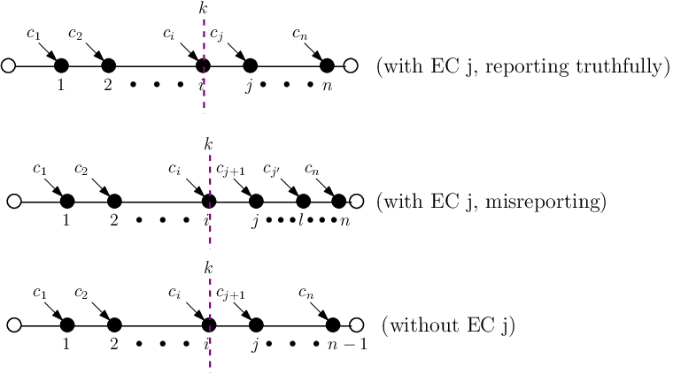
Refer to caption
Fig. 10: Pictorial representation

It is to be noted that, if the EC j reports a large deviation in his cost cjc_{j} i.e.i.e. cj′c_{j^{\prime}} in this case it will belong to losing set and will still appear after EC i as shown in Figure 10. As the ECs are sorted based on the marginal contribution per cost, so we can write:

𝓜𝓒i​(Γi−1)ci≥𝓜𝓒j​(Γi−1)ci⇒cj′≤𝓜𝓒j​(Γi−1)⋅ci𝓜𝓒i​(Γi−1)\frac{\boldsymbol{\mathcal{M}}_{\boldsymbol{\mathcal{C}}_{i}}(\varGamma_{i-1})}{c_{i}}\geq\frac{\boldsymbol{\mathcal{M}}_{\boldsymbol{\mathcal{C}}_{j}}(\varGamma_{i-1})}{c_{i}}\Rightarrow c_{j^{\prime}}\leq\frac{\boldsymbol{\mathcal{M}}_{\boldsymbol{\mathcal{C}}_{j}}(\varGamma_{i-1})\cdot c_{i}}{\boldsymbol{\mathcal{M}}_{\boldsymbol{\mathcal{C}}_{i}}(\varGamma_{i-1})}

and cj′≤𝓜𝓒j​(Γi−1)⋅ci𝓜𝓒i​(Γi−1)=𝓒jic_{j^{\prime}}\leq\frac{\boldsymbol{\mathcal{M}}_{\boldsymbol{\mathcal{C}}_{j}}(\varGamma_{i-1})\cdot c_{i}}{\boldsymbol{\mathcal{M}}_{\boldsymbol{\mathcal{C}}_{i}}(\varGamma_{i-1})}=\boldsymbol{\mathcal{C}}_{j}^{i}. From above we have got the relation 𝓒ji≤cj\boldsymbol{\mathcal{C}}_{j}^{i}\leq c_{j}. This will lead to cj′≤𝓒ji≤cjc_{j^{\prime}}\leq\boldsymbol{\mathcal{C}}_{j}^{i}\leq c_{j}. The EC j is paid less than the actual cost.

Case 2: When EC j is in winning set.

If the EC j shows a deviation in his cost such that cj′>cjc_{j^{\prime}}>c_{j} and the current position of the EC j remains unchanged. In this situation, it can still be considered in the winning set. It is to be noted that, if the EC j reports a large deviation in his cost cjc_{j} i.e.i.e. cj′c_{j^{\prime}} in this case it will belong to losing set and will appear after EC i as shown in Figure 11. Utilizing the definition of the marginal contribution per cost sorting and figure above:

𝓜𝓒j​(Γl−1)cj≥𝓜𝓒i​(Γi−1)ci⇒cj≤𝓜𝓒j​(Γl−1)⋅ci𝓜𝓒i​(Γi−1)=𝓒jl\frac{\boldsymbol{\mathcal{M}}_{\boldsymbol{\mathcal{C}}_{j}}(\varGamma_{l-1})}{c_{j}}\geq\frac{\boldsymbol{\mathcal{M}}_{\boldsymbol{\mathcal{C}}_{i}}(\varGamma_{i-1})}{c_{i}}\Rightarrow c_{j}\leq\frac{\boldsymbol{\mathcal{M}}_{\boldsymbol{\mathcal{C}}_{j}}(\varGamma_{l-1})\cdot c_{i}}{\boldsymbol{\mathcal{M}}_{\boldsymbol{\mathcal{C}}_{i}}(\varGamma_{i-1})}=\boldsymbol{\mathcal{C}}_{j}^{l}

and for the case when the EC j deviates, then

𝓜𝓒i​(Γi−1)ci≥𝓜𝓒j​(Γt−1)cj′⇒cj′≥𝓜𝓒j​(Γt−1)⋅ci𝓜𝓒i​(Γi−1)=𝓒jl\frac{\boldsymbol{\mathcal{M}}_{\boldsymbol{\mathcal{C}}_{i}}(\varGamma_{i-1})}{c_{i}}\geq\frac{\boldsymbol{\mathcal{M}}_{\boldsymbol{\mathcal{C}}_{j}}(\varGamma_{t-1})}{c_{j^{\prime}}}\Rightarrow c_{j^{\prime}}\geq\frac{\boldsymbol{\mathcal{M}}_{\boldsymbol{\mathcal{C}}_{j}}(\varGamma_{t-1})\cdot c_{i}}{\boldsymbol{\mathcal{M}}_{\boldsymbol{\mathcal{C}}_{i}}(\varGamma_{i-1})}=\boldsymbol{\mathcal{C}}_{j}^{l}

Now, if EC j deviates by large amount then it will belong to the losing set. From above two equations it is clear that no matter what cost EC j is bidding, he will be paid 𝓒jl\boldsymbol{\mathcal{C}}_{j}^{l}.

Refer to caption
Fig. 11: Pictorial representation

Hence, considering Case 1 and Case 2 it can be concluded that EC jj does not gain by overbidding there true cost. In similar fashion, we can write the above mentioned equation for any position i before k and in the same way we can prove that 𝓒ji≤cj\boldsymbol{\mathcal{C}}_{j}^{i}\leq c_{j}. Hence, max\max operator will still endure that if any agent jj deviates and wins, then his payment will be less than the true cost and hence deviation may not give any gain.

Hence, the theorem is proved. ∎

VI Performance Evaluation

We compared our proposed mechanisms against the benchmark mechanism (random mechanism). In this, the doctors are selected randomly and are paid their declared cost. We have utilized the coverage model for the first fold of our hiring problem. The performance metric includes the Interested doctors set size, and Number of doctors hired. The unit of cost and budget is $.

VI-A Simulation set-up

For our simulation purpose, a social graph is generated randomly using Networkx package of python. It consists of 1000 nodes (doctors) and approximately 28,250 edges. The maximum and minimum degree a node can have is 10% and 1% of the total available nodes respectively. The cost of each node as initial adapter is uniformly distributed over [30,50][30,50], the cost of consultancy is uniformly distributed over [35,50][35,50], and quality is uniformly distributed over [20,50][20,50]. The budget is considered in range [100,1000][100,1000].

VI-B Result analysis

The simulation results shown in Figure 13 shows the comparison of the interested doctors set size i.e.i.e. the number of doctors acting as leaders and the number of doctors informed by the leaders about the hiring concept.

Refer to caption
Fig. 12: Interested doctors set size with budget 𝓑∈[100,1000]\boldsymbol{\mathcal{B}}\in[100,~1000]
Refer to caption
Fig. 13: Hired doctors with budget 𝓑′∈[100,1000]\boldsymbol{\mathcal{B}^{\prime}}\in[100,~1000]

It is seen in Figure 13 that the interested doctors set size in case of NoTBC mechanism is higher than TBC mechanism and random mechanism. This nature of NoTBC mechanism is obvious due to the fact that the mechanisms (NoTBC-LI and NoTBC-DS) are utilizing almost the complete quota of the available budgets whereas TBC mechanism is utilizing only a part of total budget. With the increase in budget, one can easily see the increasing gap between NoTBC mechanism and TBC mechanism. It can be seen evidently in Figure 13 that the number of doctors hired in case of NoTBC mechanism is higher than TBC mechanism and random mechanism. Similar reasoning can be given as above.

VII Conclusions and future works

In this paper, we have addressed the problem of hiring the doctors from outside of the hospital when a patient is constrained by budget. Designing a more general mechanism in this environment for the set-up consisting of multiple patients say n (each patient is associated to different hospitals) and m doctors can be thought of as the future work.

Acknowledgment

We would like to thank Prof. Y. Narahari and members of the Game Theory Lab. at IISc Bangalore; Ministry of Electronics and Information Technology (MeitY) Government of India and Media Lab Asia (YFR fellowship grant under Vivsvesvaraya PhD scheme), and Government of India Ministry of Human Resource Development (Institute scholarship).

References

  • [1] F. Guerriero and R. Guido, “Operational research in the management of the operating theatre: A survey,” Journal of health care management science, vol. 14, no. 1, pp. 89–114, March 2011.
  • [2] B. Cardoen, E. Demeulemeester, and J. Belien, “Operating room planning and scheduling: A literature review,” European journal of operational research, vol. 201, no. 3, pp. 921–932, March 2010.
  • [3] I. Berrada, J. A. Ferland, and P. Michelon, “A multi-objective approach to nurse scheduling with both hard and soft constraints,” Socio-economic planning sciences, vol. 30, no. 3, pp. 183–193, 1996.
  • [4] C. V. Huele and M. Vanhoucke, “Analysis of the integration of the physician rostering problem and the surgery scheduling problem,” Journal of medical systems, vol. 38, no. 6, pp. 1–16, May 2014.
  • [5] J. B. Starren, T. S. Nesbitt, and M. F. Chiang, “Telehealth,” Journal of biomedical informatics, pp. 541–560, 2014.
  • [6] V. K. Singh, S. Mukhopadhyay, N. Debnath, and A. M. Chowdary, “Auction aware selection of doctors in e-healthcare,” in Proceeding of 17t​h17^{th} Annual International Conference on E-health Networking, Application and services (HealthCom). Boston, USA: IEEE, 2015, pp. 363–368.
  • [7] V. K. Singh, S. Mukhopadhyay, and R. Das, “Hiring doctors in e-healthcare with zero budget,” in Advances on P2P, Parallel, Grid, Cloud and Internet Computing: Proceedings of the 12t​h12^{th} International Conference on P2P, Parallel, Grid, Cloud and Internet Computing (3PGCIC-2017), F. Xhafa, S. Caballé, and L. Barolli, Eds. Cham: Springer International Publishing, 2018, pp. 379–390.
  • [8] V. K. Singh, S. Mukhopadhyay, A. Sharma, and A. Roy, “Hiring expert consultants in e-healthcare: A two sided matching approach,” CoRR, vol. abs/1703.08698, 2017.
  • [9] H. Chan and J. Chen, “Provision-after-wait with common preferences,” in Proceedings of the International Conference on Autonomous Agents and Multiagent Systems, ser. AAMAS ’16. Richland, SC: IFAAMAS, 2016, pp. 278–286.
  • [10] B. Cardoen, E. Demeulemeester, and E. Frank, “Operating room planning and scheduling problems: A classification scheme,” International journal of health management and information, vol. 1, no. 1, pp. 71–83, 2010.
  • [11] Y. W. Ko, D. H. Kim, S. Uhmn, and J. Kim, “Nurse scheduling problem using backtracking,” Advanced science letters, vol. 23, no. 4, pp. 3792–3795, April 2017.
  • [12] M. W. Carter and S. D. Lapiere, “Scheduling emergency room physicians,” Health care management science, vol. 4, no. 4, pp. 347–360, December 2001.
  • [13] F. Dexter and A. Macario, “When to release allocated operating room time to increase operating room efficiency,” Anesthesia and analgesia, vol. 98, no. 3, pp. 758–762, March 2004.
  • [14] R. M. Pottayya, J. C. Lapayre, and E. Garcia, “An adaptive videoconferencing framework for collaborative telemedicine,” in Proceedings 31s​t31^{st} International Conference on Advanced Information Networking and Applications (AINA), Taipei, Taiwan, March 2017, pp. 197–204.
  • [15] C. Tekin, O. Atan, and M. V. D. Schaar, “Discover the expert: Context-adaptive expert selection for medical diagnosis,” IEEE transactions on emerging topics in computing, vol. 3, no. 2, pp. 220–234, June 2015.
  • [16] Y. Singer, “How to win friends and influence people, truthfully: Influence maximization mechanisms for social networks,” in Proceedings of the 5t​h5^{th} International Conference on Web Search and Data Mining, ser. WSDM ’12. New York, NY, USA: ACM, 2012, pp. 733–742.
  • [17] ——, “Budget feasible mechanisms,” in Proceedings of 51s​t51^{st} Annual Symposium on Foundations of Computer Science (FOCS), Oct 2010, pp. 765–774.
  • [18] S. Khuller, A. Moss, and J. S. Naor, “The budgeted maximum coverage problem,” Information processing letters, vol. 70, no. 1, pp. 39–45, April 1999.