Notes on Anomaly Induced TransportThanks: Based on lectures presented at 56. Cracow School on Theoretical Physics, May 24 - June 1 2016, Zakopane, Poland and the APCTP focus workshop on Holography and Topology of Quantum Matter, August 22 - August 29, 2016, Pohang, Korea.
Abstract
Chiral anomalies give rise to dissipationless transport phenomena such as the chiral magnetic and vortical effects. In these notes I review the theory from a quantum field theoretic, hydrodynamic and holographic perspective. A physical interpretation of the otherwise somewhat obscure concepts of consistent and covariant anomalies will be given. Vanishing of the CME in strict equilibrium will be connected to the boundary conditions in momentum space imposed by the regularization. The role of the gravitational anomaly will be explained. That it contributes to transport in an unexpectedly low order in the derivative expansion can be easiest understood via holography. Anomalous transport is supposed to play also a key role in understanding the electronics of advanced materials, the Dirac- and Weyl (semi)metals. Anomaly related phenomena such as negative magnetoresistivity, anomalous Hall effect, thermal anomalous Hall effect and Fermi arcs can be understood via anomalous transport. Finally I briefly review a holographic model of Weyl semimetal which allows to infer a new phenomenon related to the gravitational anomaly: the presence of odd viscosity.
1 Introduction
Symmetries are one of the most fundamental concepts of modern physics. The same is true for quantum theory. However, sometimes these two are in conflict with each other. More precisely a symmetry present on the level of classical Lagrangian might not be compatible with quantum theory. When this happens we speak of a quantum anomaly [1, 2, 3].
What shall concern us here specifically are chiral anomalies. These are intimately related to the fact that in even space-time dimensions the Lorentz group has two unitarily inequivalent spinor representations giving rise to left- and right-handed spinors. For massless fermions independent phase rotations of left- and right-handed spinors are symmetries of the classical theory. On the quantum level at best one linear combination of these two symmetries can be preserved.
In the realm of high energy physics the prime example of a physical phenomenon induced by the incompatibility of chiral symmetries with quantum theory is the decay of the neutral pion into two photons. Besides explaining such otherwise forbidden (or strongly suppressed) processes in particle physics anomalies also place very stringent consistency conditions on gauge theories. Gauging an anomalous symmetry leads to violation of unitarity. The divergence of the current couples to the longitudinal gauge degrees which normally corresponds to zero norm states. Anomalies lead to scattering of physical states into zero norm states and therefore destroy unitarity. Alternatively one can allow a mass term for the gauge field, then however renormalizability is lost [4]. Even when the symmetries are not gauged anomalies do place very stringent conditions on the strong dynamics of gauge theories. ’t-Hooft [5] argued that the spectrum of chiral fermions in a gauge theory is protected by this type of anomalies appearing in global symmetries. These constraints of “anomaly matching” between (weakly coupled) high energy theories and (strongly coupled) low energy effective theories can be exploited to get a handle on otherwise difficult to understand strong gauge dynamics. The power of anomalies lies in the fact that they are subject to a non-renormalization theorem [6] stating that the anomaly is exact as an operator relation at one loop.
In the recent years anomalies have also emerged as the leading concept that allows to understand (and discover) unusual transport phenomena of quantum many body physics involving chiral fermions. In high energy physics this is relevant to the physics of the quark gluon plasma as created in heavy ion collisions at RHIC and LHC. Anomalies have been invoked to predict charge asymmetries in the final state of a heavy ion collision [7, 8, 9] and indeed charge asymmetries consistent with the prediction of anomalous transport theory have been detected in experiments at RHIC and LHC [10, 11]. In astrophysics anomalous transport phenomena have been suggested to explain the sudden acceleration suffered by neutron stars at birth (neutron star kicks) [12] in cosmology as origin of primordial magnetic fields [13].
But (and probably somewhat surprisingly) anomalous transport phenomena are about to play also a lead role in condensed matter physics. It is already well established that quantum Hall physics (see [14] for a recent review) can be described in a quantum field theory language via anomaly inflow [15] from bulk to boundary of a topologically nontrivial insulator. More recently also the bulk physics of three (space) dimensional metals has been argued to be governed by chiral anomalies, e.g. via the phenomenon of negative magnetoresistivity. Of course these are not ordinary metals but very special ones in which the Fermi surface lies at or very near linear band touching points [16, 17, 18]. In these cases the effective low energy electronic excitations near the band touching points are chiral fermions and the theory of anomalous transport can be applied to infer and describe a variety of exotic transport phenomena.
The aim of these lectures is to give an introduction to the subject with emphasis on making the underlying quantum field theoretical concepts as clear as possible. If one understands as a quantum field theory a prescription of how to compute correlation functions of (gauge invariant) operators then string theory derived holography needs also to be taken into account. Indeed holography has played a major role in the modern area of anomalous transport and many subtleties arising when dealing with anomalies are most easily understood using the holographic framework [19, 20, 21, 22, 23, 24].
These notes are organized as follows: in section 2 we will review chiral triangle anomalies. Particular emphasis will be made on the ambiguities in the regularization procedure and how they can be fixed by physical constraints. This will lead to the concepts of covariant and consistent anomalies [25]. In section two we will discuss the Landau level quantization of chiral fermions. We will see how the (covariant) anomaly arises as a conflict between normal-ordering and spectral flow. We will emphasize that the spectral flow needs to be supplemented with boundary conditions at a cutoff in momentum space and from this we will give a physical picture of the consistent anomaly via anomaly inflow. In section 3 will use the Landau level quantization to derive the anomalous transport formulas for chiral magnetic and chiral vortical effects. In section 4 will briefly review relativistic hydrodynamics with anomalies and the fact that the contribution of the (mixed) gravitational anomaly cannot be fixed by hydrodynamic arguments alone due to a mismatch in the number of derivatives in the transport phenomena and the anomaly. Section 5 will introduce a simple holographic model allowing to make the relation between anomalies and transport coefficients manifest. The derivative mismatch for the gravitational anomaly contribution is overcome in holography by taking derivatives in the holographic direction. Section 6 is devoted to the physics of Weyl semi-metals. After a quick introduction we will show how almost all exotic Weyl semimetal phenomenology can be understood from anomalous transport theory as outlined in the previous sections. These include negative magnetoresistivity in magnetic fields, in axial magnetic fields, thermal hall transport and the appearance of edge currents related to Fermi arcs. Section 7 will then briefly review a recently developed holographic model of Weyl semimetal and show that it can be used to derive a new transport phenomenon related to the gravitational anomaly not contained in the ones discussed previously: odd viscosity.
2 Triangle Anomalies
Let us start with a massless Dirac fermion
| (1) |
In a chiral (Weyl-) representation of the -matrices such that
| (2) |
We define the left- and right-handed spinors via the projector . The massless Dirac equation
| (3) |
has two independent symmetries acting as and which we denote with . The corresponding conserved currents are , and on the level of classical field theory
| (4) |
For future reference let us also write down the Hamiltonians for left- and right-handed fermion in momentum space
| (5) |
which will be convenient once we discuss Weyl semi-metals.

2.1 Chiral Anomalies
Let us focus now on a single chiral fermion. We can define the generating functional that allows to compute arbitrary n-point functions of the current via gauging. We introduce an external gauge field and write the action as
| (6) |
The quantum effective action (1-particle irreducible) is defined as11 1 More precisely one might use the action in the exponent of the path integral to get a well defined Dirac operator.
| (7) |
Since the action is invariant under the transformation for arbitrary functions it follows seemingly that the quantum action is invariant and obeys
| (8) |
By construction functional variation with respect to the gauge field inserts the operator . Therefore gauge invariance suggests that as an operator equation, i.e. that arbitrary correlation functions with one insertion of the divergence of the chiral current should vanish. As is well-known this is not true and the obstruction of defining such a gauge invariant quantum action is the chiral anomaly.
Let us reconsider the anomaly in the elementary triangle diagram of three chiral currents. Applying the usual Feynman rules to the triangle diagrams in figure 1 we find the three point amplitude ()
| (9) |
Details of the evaluation of this diagram are discussed in many textbooks such as [26] so we will only sketch the most important features. First we note that the parity odd part of the projection operator is relevant. So we replace it with , then use . Computing the divergence
| (10) |
Because of Lorentz symmetry the integrals has to be proportional to either or and these combinations vanish once contracted with the epsilon tensor. On the other handed
| (11) |
If the integrals were well defined we could make the substitution in the second integral. The single integral is however linearly divergent and has to be defined properly. Vanishing of depends now on the way we have labeled the internal loop momentum. Any other choice is just as good. The most general choice is where are arbitrary real numbers. Now the integrals can be evaluated in a Lorentz invariant fashion. All divergences cancel but the final result is undetermined because of the ambiguity in labeling the internal loop variable (since the gamma matrix trace gives an epsilon tensor it is only the anti-symmetric combination of external momenta that contributes). One finds
| (12) | ||||
| (13) | ||||
| (14) |
Thus the one-loop three point function of three chiral currents is finite but undetermined. This poses the question what is the correct value of ? Not too surprisingly the answer to this question is: it depends! It does depend on the physical constraints the three point function shall obey.
First let us go back to the quantum effective action and demand that the three point function of currents is
| (15) |
Since the order of differentiation does not play any role we must impose Bose symmetry on the external legs, all three vertices couple in precisely the same way to the gauge field. This imposes . If we express the anomaly now in terms of the current and the external gauge fields we find
| (16) |
For reasons to be explained shortly this is called the consistent form of the anomaly.
On the other hand we might be interested to define a quantum operator that has nice properties with respect to gauge transformations. More precisely we would like to think of the current as an object that couples covariantly (i.e. without anomaly) to the external gauge fields. This singles out one particular vertex and demands that the divergence on the other two vertices vanishes. The solution for this covariant definition of current is and the anomaly is now
| (17) |
This looks almost the same as before except for the overall factor of in the anomaly. It is called the covariant anomaly. Since now we have treated the vertices in different ways it is clear that this definition of three point amplitude violates the Bose symmetry (15). This means that the covariant current obeying the covariant anomaly equation (17) can not be thought of as a functional variation of a quantum effective action22 2 It also appears as the edge current in systems where the anomaly is localized on a co-dimension one boundary and canceled via a higher dimensional Chern-Simons term as in quantum Hall systems. See also [27] for an application of this in the context of anomalous transport theory.. It might look surprising that we obtained two different answers for the divergence of “the current” by imposing two different but equally reasonable looking conditions. Later when discussing anomalies and transport we will suggest physical interpretations of these different quantum operators, the consistent () and the covariant () currents.
2.2 Axial Anomaly
On the level of classical physics a Dirac fermion is the direct sum of left- and a right-handed chiral fermions, . Anomalies pose a restriction on the possibility of defining chiral fermions in the quantum theory. Not too surprisingly they also have implications on this direct sum. Let us proceed naively and simply define the quantum theory of a Dirac fermion as the quantum theory of a left-handed and a right-handed fermion. We want to keep the external gauge fields distinguishable, i.e. we introduce left- and right-handed gauge fields coupling to the chiral currents independently. We define vector and axial currents via
| (18) | ||||
| (19) |
and a basis of vector-like and axial gauge fields
| (20) | |||
| (21) |
We can just add and subtract equations (16) to find
| (22) | ||||
| (23) |
where and . We have chosen to express this in terms of the consistent currents. The result is the same up to an overall factor of for the covariant currents. Equation (22) looks troublesome: eventually one would like the vector current to play the role of the electric current that couples to a dynamical gauge fields. Even without quantizing the gauge fields one should expect that the electric current acts as source of Maxwell’s equations
| (24) |
This is only consistent if the divergence of the vector current vanishes, since . One might say that this is still true in the absence of axial gauge fields and that indeed in nature on a fundamental level axial gauge fields do not exists. However one should keep in mind that equation (22) is just a short form for insertions of the divergence of the vector current in correlation functions. Its meaning is that there is a three point function of a divergence of a vector current with an axial current and another vector current that does not vanish. Furthermore as we will see later in Weyl semi-metals such axial gauge fields do arise quite naturally in the low energy effective description of their electronics. So we need to solve this problem of non-conservation of the vector current. Happily this has been done long time ago [28] by noticing that once gauge invariance is lost, nothing prevents us from introducing additional (non-gauge invariant) local counterterms to our quantum action. These are called Bardeen counterterms and they redefine the quantum action as follows
| (25) |
If we now compute the (consistent) currents as variation of the effective action with respect to the gauge fields and chose and we find
| (26a) | ||||
| (26b) | ||||
This form of the anomaly is the consistent axial anomaly. The Bardeen counterterms guarantee that a conserved vector current can be defined always, independently of the chosen regulator. We have not specified the regulator but generically a left-right symmetric regularization would not give a conserved vector current. On the other hand manifestly gauge invariant regulators such as dimensional reduction automatically produce the Bardeen counterterms in the effective action and nothing has to be added “by hand”. The particular Chern-Simons terms that are the Bardeen counterterms exist only if there are at least two independent gauge fields. That makes the nature of the axial anomaly as a mixed anomaly manifest. The precise statement of the axial anomaly is that there is no quantum theory in which both the axial and the vector like currents are conserved at the same time.
2.3 Wess-Zumino consistency condition
So why the anomaly is called consistent? To understand this we need some more formalism. Our object of interest is the quantum effective action (for simplicity of notation we go back to the case of only one abelian gauge field). An anomaly is a non-invariance of the effective action under a gauge transformation. The gauge transformation can be written as a functional differential operator and the anomaly is expressed as
| (27) |
The right hand side arises because there is no regularization scheme that is compatible with the symmetry. It is a remnant of the regularization and remains even if we renormalize and take the regulator to infinity. That makes it intuitively clear that it has to be the integral of a local expression in the field . On the other hand the quantum effective action arises by integrating out massless (chiral) fermions and is essentially a non-local expression. We further observe that the gauge transformations have to obey the gauge algebra which in our simple example means that two gauge transformations with different gauge parameters have to commute.
| (28) |
It follows now that the anomaly has to fulfill
| (29) |
This is the Wess-Zumino consistency condition. A more geometric formulation can be given with one more piece of formalism. Let us promote the gauge parameters to a Grassmann valued field called the ‘‘ghost’’33 3 In the path integral quantization of non-abelian gauge theories this is the Fadeev-Popov ghost that arises in defining the measure.. It is useful to have the analogy of the exterior derivative and the formalism of differential forms in mind, e.g. the field strength of a gauge field (1-form) is defined as the exterior derivative . In an analogous way let us introduce an exterior derivative on field space
| (30) |
Which is nothing but a gauge transformation with the Grassmann valued ghost field as gauge parameter. It is called the BRST operator44 4 See [29] for a recent review.. As one can check easily it is nilpotent . The anomaly can now be written as
| (31) |
We can think of the anomaly as a one-from on field space (a local integrated polynomial of the field , one ghost field and a finite number of derivatives, i.e. having ghostnumber one). The Wess-Zumino consistency condition is the fact that the anomaly is a closed one-from with respect to the BRST operator
| (32) |
Here we have included the condition that it should not be possible to write the anomaly as the BRST variation of an integral of local term of ghostnumber zero. If that were the case we could just add as counterterm of the effective action and get a new redefined and BRST (gauge-) invariant quantum action. This maps the anomaly to a cohomology problem: the consistent anomaly is a non-trivial element of the BRST cohomology on the space of local integrated monomials in the fields at ghostnumber one. Finally let us note that all this formalism can be extended in full generality to non-abelian gauge algebras.
2.4 Covariant Anomaly
OK, so now we know that the consistent anomaly is a solution to the consistency condition. But what is the covariant anomaly? Well, we observe that the consistent current defined as the functional derivative of the quantum action is not a gauge invariant operator if there is an anomaly. Using we find
| (33) |
where in in the expression on the right we have specialized to one chiral fermion again. We already know that in the triangle diagram we can put all the anomaly into a single vertex. So it must be possible to define a current with covariant couplings to the external legs. In particular we should demand from this quantum operator even in the presence of an anomaly.
From (33) it is easy to see that by adding a Chern-Simons current to the consistent current we can define
| (34) |
Adding the Chern-Simons current to the consistent current we can construct the covariant current. The defining characteristics of this current are that it is invariant under all the gauge transformation, even the anomalous ones, and that it can not be obtained from variation of an action with local counterterms. We emphasized this already in the analysis of the triangle diagram but now we can also see it from he Chern-Simons current in (34). We can compute the anomaly in the covariant current (it is a covariant object under the anomalous gauge transformations but it does have an anomaly by itself)
| (35) |
As expected this is of the consistent anomaly.55 5 We could also define a conserved current by adding the Chern-Simons current with an appropriate coefficient. Such a current is then neither consistent (variation of an effective action) nor gauge invariant.
We can go through the same exercise in the case of the axial anomaly and construct the covariant vector and axial currents. With our canonical choice of taking the vector current explicitly conserved we have
| (36a) | ||||
| (36b) | ||||
Note that only the axial gauge potential enters these expressions. This is a reflection of the fact that we have chosen to put all the anomaly into the axial current. For future reference let us also write down the covariant vector and axial anomaly
| (37a) | |||||
| (37b) | |||||
The covariant anomaly looks completely vector-axial symmetric once we express it in therms of electric and magnetic fields. Generally there always exists Chern-Simons currents that can be added to the consistent currents making the resulting covariant current a covariant object under all gauge transformations. They are also known as Bardeen-Zumino polynomials (not to be confused with the Bardeen counterterms). The theory of covariant and consistent anomalies goes back to [25].
2.5 Gravitational Anomaly
There is one more anomaly that appears in the triangle diagram of one chiral current and two energy-momentum tensors. This is the gravitational contribution to the chiral anomaly (also mixed gauge-gravitational) anomaly [30, 31, 32]. It is by nature a mixed anomaly and therefore one can always use Bardeen counterterms to shift the anomaly between the involved symmetries. Note that the Bardeen counterterms have the form connectionconnectionfield-strength. In the case of gravity the connection (=gauge field) is the Levi-Civita connection and the field strength is the Riemann tensor. On a fundamental level, gravity is always gauged in nature and that implies that there should not be any anomaly in the diffeomorphism symmetry. So it is customary to shift the anomaly completely into the chiral current in which case it takes the form
| (38) |
for a single chiral fermion. Again one can find a covariant form of this anomaly applying the principles outlined in the previous subsection. While this looks a rather straightforward application of the principle that anomalies are contractions of field strength tensors with the epsilon tensor there is at least one clear difference: the usual chiral and axial anomalies are expressions involving two derivatives whereas the gravitational anomaly involves four derivatives.
2.6 Anomaly coefficients
Anomalies are subject to non-renormalization theorems. The anomaly coefficient is exact at the one loop level. So one can infer the presence of an anomaly by analyzing the triangle diagram with generic currents at the vertices. Let us assume a generic symmetry group generated by matrices such that . Chiral anomalies are present if the anomaly coefficient
| (39) |
does not vanish. Here the sums run over the species of left- and right-handed fermions and are the representations of left- and right-handed fermions and the curly bracket is the anti-commutator. In the case when all symmetries are abelian this boils down to sums over triple products of charges
| (40) |
A mixed gravitational anomaly is present if
| (41) |
is different from zero. We call and the chiral and gravitational anomaly coefficients. Note that is completely symmetric. By means of adding Bardeen counterterms one can cancel some of the consistent anomalies. This is precisely the case of the axial anomaly where but the consistent vector current is conserved.
3 Landau Levels and anomalies
We now study chiral fermions in a magnetic field66 6 A recent review on quantum field theory in magnetic field backgrounds is [33]. The Weyl equation is
| (42) |
and the covariant derivative is (absorbing the electric charge into the definition of the gauge field). The magnetic field is taken to point in the -direction and the gauge field is chosen . The Weyl equation is
| (43) |
We now use the fact that the differential equation depends explicitly only on and not on the other coordinates so we can use the ansatz to find the matrix equation
| (44) |
For there is a simple solution and whereas the corresponding solution with and is non-normalizable. This is the Lowest Landau with , where is the eigenvalue of the spinor wave function of . For a chiral fermion of opposite chirality one finds that the normalizable solution has and . The lowest Landau level disperses linearly
| (45) |
with the sign determined by chirality. The rest of the spectrum arranges into Landau levels of positive and negative energies given by
| (46) |
with . The Weyl equation in a magnetic field can be separated into a plane wave and a harmonic oscillator corresponding the the degrees of freedom along and transverse to the magnetic field. Accordingly the momentum along the magnetic field is still a good quantum number but the momenta in the plane transverse the the magnetic field are replaced by just the harmonic oscillator quantum number . In our gauge choice the momentum in direction parametrizes the degeneracy of the Landau levels of states per unit area. The spectrum is sketched in figure 2.
Let us apply now the standard argument that allows to derive the chiral anomaly from spectral flow [34]. In addition to the magnetic field we switch on a parallel electric field . This field will pump momentum into the system according to Newtons law . In the Dirac sea of the higher Landau levels all states are occupied and a fermion has no available state to move to77 7 In condensed matter physics it is known that fully occupied bands do not produce an electric current (if not for topological reasons).. For the lowest Landau level there is something more going on. We assume, as usual in quantum field theory, that the infinite Dirac sea of negative energy states is subtracted via a normal ordering prescription. The electric field pumps momentum into the system and shifts the states in the Dirac sea of the of the lowest Landau level to positive momentum! Occupied states just below the normal ordered vacuum are shifted into empty states just above the vacuum. This is particle creation out of the vacuum. We can also compute the rate of particle creation. The density of states for a one dimensional chiral fermion (such as the fermions in the lowest Landau level) is and their degeneracy is . If we combine this with the Lorentz force we find
| (47) |
But this is just a Lorentz non-covariant version of the anomaly equation !. So now the anomaly has been recovered from rather elementary quantum mechanics of a singe Weyl fermion without any fancy quantum field theory. Why was this so easy and where does quantum field theory hide? It hides in two aspects: first we assumed a notion of normal ordered vacuum which is our trick to subtract the infinite Dirac sea. The anomaly is then the incompatibility between the spectral flow and our normal ordering prescription. There is another aspect to it: where do all the fermions come from? Well in this picture we do not really have to ask this question since the Dirac sea is infinite and any finite amount of states that we pull out of the vacuum will not be able to deplete the infinite supply of states in the Dirac sea88 8 Sometimes this is compared to the Hilbert Hotel with an infinite number of rooms. Any new arrival can be accommodated by simply asking the occupants in room number to switch to room number leaving the room number available. In quantum field theory there is another ingredient that we will have to take into account eventually: a cutoff has to be introduced at intermediate stages of the calculations. This will turn out to be an essential ingredient to the proper spectral flow picture of the axial anomaly. For the moment we want to point out that the prefactor of the anomaly obtained via the spectral flow argument is the one of the covariant anomaly. In hindsight this is not surprising, since we assumed that our chiral fermions couple covariantly to the external fields (i.e. we assumed the usual form the Lorentz force.) The spectral flow picture of the chiral anomaly is sketched in figure 3.
Let us now combine left- and right-handed Weyl fermions to get an idea of the spectral flow of the axial anomaly. States are created and annihilated since for each right-handed fermion pulled out of the vacuum there is a left-handed particle that is pushed further down into the Dirac sea. The total anomaly is
| (48) |
For this particular case we can actually not decide if this is the covariant or the consistent anomaly (22) with conserved vector current. Both anomalies have the same coefficient, which is not surprising since the vector current actually is anomaly free and trivially a covariant object under (vector-like) gauge transformations. The spectral flow picture for the axial anomaly is depicted in figure 4.
Now let us see how we can understand the spectral flow when we switch on parallel axial electric field and usual (vector-like) magnetic field. The spectral flow picture tells us that both, left-handed and right-handed particles are created out of the vacuum. This indeed looks problematic since it would mean that vector-like charge (which eventually we want to identify with the electric charge) is not conserved. To understand better what is going on we need to keep in mind that the axial field is of different nature than the true gauge field because of the anomaly. Whereas the proper gauge field is not an observable itself is in principle observable. A pure gauge does not decouple from the theory, rather it couples to the anomaly. It is therefore natural to impose the boundary condition at infinity, can be different from zero only in a compact domain. Let us imagine but constant in a slab . Then at there is a strong gradient of which is nothing but an axial electric field . If a parallel (vector-like) magnetic field is present the covariant anomaly (37a) gets excited and creates charge out of the vacuum at but destroys charge in equal amounts at . So that’s already good since globally no net charge is created. But it is not yet good enough! Charge conservation is a local equation and tells us that charge can only leave or enter a bounded region via inflow or outflow of current. So even with the boundary condition we still violate local charge conservation. This is where the Bardeen-Zumino polynomial comes to rescue! The relation between the covariant and conserved consistent current (36a) tells us that in a region with non-vanishing axial vector and simultaneous presence of vector-like field-strength a Chern-Simons current is created. This current is precisely such that it provides the inflow guaranteeing local charge conservation. The spectral flow picture of this consistent picture of the “anomaly” is depicted in figure 5.
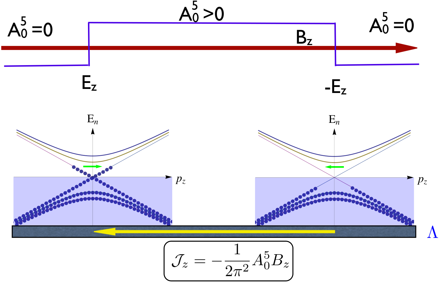
The fermions following the spectral flow do not really just move out to arbitrary high momentum. In quantum field theory we always have to include a finite cutoff at intermediate stages of our calculations. So with the regulator in place the fermions subject to spectral flow hit the cutoff and we need to tell them what they shall do at the cutoff by imposing boundary conditions in momentum space. Of course the correct boundary condition for a conserved electric current is that as soon as the fermions hit the cutoff they generate a current in space transporting precisely the right amount of charge from the region of negative axial electric field to the region of positive axial electric field. This inflow guarantees local charge conservation. Of course we could also impose some sort of leaky boundary conditions in which we allow some of the charge to vanish into to the region beyond the cutoff. On the level of the effective action the boundary conditions at the cutoff are parametrized by the Bardeen counterterms (25). This is basically the same mechanism that is behind the anomaly inflow mechanism of [15]. The only difference being that now the bulk is not gapped99 9 In view of applications in condensed matter we might propose the maps Callan-Harveytopological insulators vs. Bardeen-Zuminotopological metals..
The Chern-Simons current generated to guarantee local charge conservation is . This looks precisely like the celebrated chiral magnetic effect, i.e. the generation of a current via magnetic field. It is only one part of the CME. So far we have assumed that our system was in a vacuum state with respect to the normal ordered vacuum, i.e. no states above the vacuum are occupied. In the region where the vacuum energies are shifted: the left-handed vacuum is shifted down by and the right-handed vacuum is shifted up by . In the next section we will study another source of magnetic (and rotation) induced currents built up by the occupied states above the normal ordered vacuum.
4 Transport from Landau Levels
For a fermion the vacuum is the state with vanishing Fermi surface. Let us now go beyond this restriction and study what happens when there is a non-vanishing Fermi surface and once we’re at it we also introduce finite temperature (so strictly speaking there is no sharp Fermi surface but it is smoothed by the temperature). To start we study what happens if we have a single chiral fermion in a magnetic field with chemical potential at temperature . Of course the charge and energy is non-vanishing and this is described by the free energy density1010 10 For completely free fermions we also could introduce independent left- and right-handed temperatures. If we understand the the expressions as lowest order in a perturbative expansion of an interacting theory only a common temperature can be defined. Local interactions can preserve separate left- and right-handed symmetries so different chemical potentials can be defined in the interacting theory. The anomaly spoils this but only in the simultaneous presence of electric and magnetic fields.
| (49) |
if the magnetic field is much smaller than Temperature and chemical potentials and by
| (50) |
for large magnetic field. The last expression is valid as long as the magnetic field induces a gap in the higher Landau levels . In that case the only states that contribute are the states in the lowest Landau level and these are effective dimensional chiral fermions. The contribution from the higher Landau levels in this regime is exponentially suppressed.
Let us compute the current in a magnetic field. First we start with the higher Landau levels. Note that the current is simply the integral over the velocity of of the particles weighted by the Fermi-Dirac distribution
| (51) |
The velocity in the higher Landau Levels is the group velocity , both particles and anti-particles contribute, the latter however with opposite sign. The integrand is an odd function of . Since the probability of finding a particle with infinite momentum is exponentially suppressed the integral is well defined and evaluates to zero. There is no current generated in the higher Landau levels.
The lowest Landau level is different. The integration region is only the positive half line and the velocity is simply depending on chirality. So we find
| (52) |
Now we remember that these states come with a multiplicity of per unit area and this give the current density
| (53) |
Finally here it is, the celebrated expression for the chiral magnetic effect: The generation of a current in a magnetic field. Many things are remarkable about this formula. First we have computed it at finite temperature but the result is completely independent of it. Only the lowest Landau level contributes, but contrary to the expression for the free energy (49) this is not an approximation valid for large field strength but it is an exact result!
Let us go a step further, let us also compute the energy current. Since we are dealing with a relativistic theory we can equally well call it the momentum density along the magnetic field. The calculation is very similar, only the lowest Landau level contributes and we find
| (54) |
giving
| (55) |
This is the chiral magnetic effect in the energy current. Now the temperature contributes but only in a very simple polynomial way!
It is a common lore in many body physics that rotation has many similarities to magnetic fields. For example the Coriolis force is similar to the Lorentz force if we identify 1111 11 Of course rotation also gives rise to a centrifugal force. It is quadratic in the angular velocity . We might try to ignore it on the grounds that it is higher order in derivatives. For relativistic, massless fermions we should replace the rest mass with the energy. Now we can calculate the current due to rotation
| (56) |
and the energy current
| (57) |
These (admittedly somewhat hand-waving) arguments give rise to the chiral vortical effects (CVE) in the current and energy current
| (58) | ||||
| (59) |
Very nice! We get currents from the lowest Landau level. This is quite interesting by itself but it gets even a bit more interesting remembering that the lowest Landau level was also responsible for the anomaly. So is there a more direct connection? And this answer is yes! As a first step let us generalize our results for single fermions to many different species of fermions and label them by an index (we can also switch to a basis with left-handed fermion only). Then assume that there is a bunch of symmetries labeled by an index under which the fermions carry charges . The chemical potential for the fermion species is then and it sees the magnetic field . The current corresponding to symmetry is likewise . Now we use the expression for the elementary chiral currents and obtain (summation over repeated indices is implied here)
| (60) | ||||||
| (61) |
Where and are the chiral and gravitational anomaly coefficients [35]. This is a hint towards the deep origin of these expression. The currents are indeed induced by the chiral and gravitational anomaly as we will discuss in the next sections. We have obtained these expressions without having to worry about regularization issues. The integrals are finite because they are damped in the UV by the exponential decay of the distribution functions. Furthermore in view of what we learned about the spectral flow we also know that naive counting of particles around the Fermi surface (or the normal ordered vacuum) gives us only the covariant current. To get the consistent current additional terms can and do arise from the Bardeen-Zumino polynomials.
Let us now specialize to the case of one Dirac fermion: we have , and . Let us study the magnetic effects and include also the Chern-Simons current from the Bardeen-Zumino polynomial, i.e. we want to write down the magnetic field induced currents in terms of the conserved consistent current.
| (62) | ||||
| (63) |
These two are are the (proper) chiral magnetic effect and the chiral separation effect (CSE). While they look very similar if written down in terms of the covariant current they are quite different once written in terms of the consistent current. There is no contribution to the CSE by any Bardeen-Zumino polynomial. Ultimately this can be traced back to the fact that it depends only on the chemical potential related to a truly conserved current. On the other hand the CME receives two contributions, one from the states that fill the energy range between the vacuum and the Fermi surface and another one that stems from the boundary conditions in momentum space and depends on the specific gauge invariant regularization. We have already mentioned that the role of is to shift the tips of the Weyl cones in opposite directions in energy. If this shift is equal to the imbalance in the chemical potentials then there is a perfect cancellation between the two terms and the CME vanishes. In fact if one defines the grand canonical ensemble for axial charge in the usual way by introducing a Hamiltonian this has the effect of achieving both effects: a non-vanishing occupation number but also a shift in the locations of the tips of the Weyl cones in precisely such a way that . This definition of equilibrium grand canonical ensemble results in a vanishing CME! The different situations of vanishing vs. non-vanishing CME are sketched in figure 6.

5 Hydrodynamics and triangle anomalies
So far we have derived the CME and the CVE (with some hand waving) only for free fermions. We need to convince ourselves that the CVE expressions have some physical meaning. We could try to do better and study an ensemble of rotating fermions, except that this is still rather ill-defined. In a relativistic theory an equilibrium ensemble with constant rotation cannot exist since at some large enough radius the tangential velocity necessarily would exceed the speed of light. In addition we need to include interactions as well. The lowest Landau level is subject to an index theorem that protects it, so we might expect that interactions don’t do modify the expressions for the CME. An effective way of studying an interacting gas or more general a fluid of chiral fermions is the formalism of hydrodynamics. Hydrodynamics is an effective field theory describing the time evolution of systems near equilibrium1212 12 Although demanding closeness to equilibrium is probably too restricted. A modern point of view is that systems even relatively far from equilibrium can be well described by hydrodynamics [36] . One assumes that locally the system equilibrates fast such that local versions of thermodynamic parameters, the temperature and the chemical potential can be defined. Intuitively thermodynamics is what is left of a system if we forget all the details that can be forgotten. That means we know nothing but the indestructible conserved charges, like energy and charges. Now we promote these to local notions of energy density and charge density. In relativistic systems we therefore need a four vector to describe the dynamics of the charge and a symmetric second rank tensor to describe the dynamics of the energy and momentum densities. Let us study energy-momentum conservation in quantum field theory. We assume a quantum action depending on a source field coupled to the energy momentum tensor. This source field is the metric. If there are no diffeomorphism anomalies this quantum action should be diffeomorphism invariant such that
| (64) |
Where we used that the metric and gauge field transform under diffeomorphisms as
| (65) | ||||
| (66) |
where the vector field is the generator of the diffeomorphism. Furthermore we identify and . Since is arbitrary we infer that the energy momentum tensor has to fulfill
| (67) |
So the energy-momentum tensor is naturally symmetric and conserved up to the terms on the right hand side. The first term represents the injection of energy and momentum by the external electric and magnetic fields. The second term vanishes if the current is conserved. When an anomaly is present it does contribute to the energy momentum conservation. Now we use our knowledge about anomalies gained in the previous sections. They come as consistent and as covariant ones and the covariant one couples only to the external field strengths but not to the external vector field . Indeed if we write the consistent current as covariant current plus Bardeen-Zumino polynomial the term proportional to the anomaly in (67) vanishes. So energy-momentum and charge conservation laws in terms of the covariant current takes the simpler form
| (68) | ||||
| (69) |
where we have also set the metric to the flat one. These are already the equations of motion for hydrodynamic effective field theory. The five equations can determine five dynamical variables which are commonly parametrized as local temperature , chemical potential and the fluid velocity obeying . Energy-momentum tensor and charge current are now expressed in terms of the local fluid variables in a derivative expansion (see [37] for a recent review of relativistic hydrodynamics)
| (70) | ||||
| (71) |
To zeroth order in derivatives
| (72) | ||||
| (73) |
The energy density, pressure and charge density are computed via thermodynamic relations from the free energy defined at equilibrium.
To first order in derivatives one has to deal with a large set of ambiguities since redefinitions of the local temperature, chemical potential and fluid velocity of the form etc. compete with the terms at higher order in derivatives. These ambiguities are fixed by a choice of frame. One of the standard frames is the so-called Landau frame, which is defined by demanding to all orders. It is also useful to define the projector transverse to the fluid velocity . Another important point is that for the covariant current only covariant field strenghts can enter the expression. It is useful to introduce electric and magnetic fields in the local rest frame and and the local vorticity . The first order terms then take the form
| (74) | ||||
| (75) |
Here is the shear viscosity, is the bulk viscosity and is the electric conductivity. The new coefficients and give room for response to external magnetic and electric fields. One more important point about hydrodynamics is that it also includes a local form of the second law of thermodynamics. One needs to define an entropy current with a non-negative divergence. Again the entropy current can be built up in a derivative expansion. It takes the form
| (76) |
where is the local entropy density and and new response coefficients. Now one demands
| (77) |
and this constrains the the transport coefficients in such way that . Surprisingly this constraint is much stronger for response coefficients due to magnetic field or rotation. In [38, 39] it was shown that these coefficients are almost completely determined by the second law (77) up to some undetermined integration constant
| (78) | ||||
| (79) | ||||
| (80) | ||||
| (81) |
Furthermore the new coefficients do not contribute to entropy production, i.e. they describe dissipationless transport. If we compare these with the expressions (60), (61) we see some similarity but also differences, the most striking is that there is no energy current. This can be traced back to the underlying choice of frame. We can go to another frame by redefining the four velocity such that the terms depending on charge , energy and pressure vanish. This can be done by redefining where
| (82) |
In this frame the anomaly related transport coefficients take the form [40]
| (83) | ||||
| (84) |
If we expand for small velocities to first order in we can identify the coefficients with (53), (55), (58), (59). This also fixes the so far undetermined constant .
The frame has a very nice physical interpretation [41]. In the presence of anomalies the chiral magnetic and chiral vortical effects give rise to dissipationless charge and energy flows. In the new frame the four velocity parametrizes then only the dissipative “normal” flow. If one allows momentum to relax e.g by placing an obstacle such as a heavy impurity into the flow then on long time scales all the normal flow will vanish described by while charge and momentum flow induced by CME and CVE are still present.
An alternative way of deriving the transport coefficients of a fluid subject to anomalies is the effective action approach [42]. Higher orders in derivatives have been studied in [43, 44].
The entropy argument fixes the dependence of the anomalous transport coefficients on the chemical potentials but not their temperature dependence. On the other hand we have seen already that the temperature dependence naturally has the gravitational anomaly coefficient attached to it. Since the gravitational anomaly is fourth order in derivatives and hydrodynamics is developed only to the one derivative level here there is no natural way it can enter here. A more general argument based on geometry was presented in [45] and a consistency condition based on the global gravitational anomaly was put forward in [46]. Probably the most straightforward way of demonstrating a direct relationship between the gravitational anomaly and the temperature dependence of anomalous transport coefficients comes from holography as we will review below.
6 Holography
The AdS/CFT correspondence or holographic correspondence [47] has developed over the last years into a very useful and powerful tool for studying strongly coupled field theories at finite temperature and density. Recent useful reviews are [48, 49]
Before discussing how holography can be used to gain insight into anomalous transport we very briefly review the basics of the AdS/CFT correspondence.
The origin of the AdS/CFT correspondence is the duality between Type IIB string theory on and supersymmetric gauge theory. The supersymmetric gauge theory is a non-abelian, four dimensional quantum field theory whose field content consists of six scalars, four Majorana fermions and a vector field. They all transform under the adjoint representation of the gauge group . It features four supersymmetries and this fixes all the couplings between the different fields. As it is a gauge theory physical observables are gauge invariant operators such as . The global symmetry group acts on the scalars and the fermions (in the spin representation of ).
The dual theory is a theory of gravity (this is what type IIB string theory is) but living in quite a few more dimensions, ten as opposed to the four the field theory knows about. But five of these ten are easily got rid off: the isometries of the part of the geometry form . The is the geometric realization of what appears as an internal, global symmetry group in the field theory.
The field theory is characterized by two parameters, the gauge coupling and the rank of the gauge group . The dual string theory has a string coupling (the amplitude for a string to split in two) and a fundamental length scale , the string scale. Furthermore the geometry is determined by a scale determining the curvature of the AdS5 as . The AdS/CFT correspondence relates these parameters in the following way:
| (85) | |||||
| (86) |
The AdS/CFT correspondence is therefore a strong weak coupling duality: for weak curvature we have large and therefore also large ’t-Hooft coupling. In this regime of weak curvature stringy effects are negligible and we can approximate the string theory by type IIB supergravity. If we furthermore take the rank of the gauge group to be very large we can also neglect quantum loop effects and end up with classical supergravity! This is the form of the correspondence most useful for the applications to many body physics: classical (super)gravity on dimensional Anti-de Sitter space.
Based on this original example we can conjecture that every theory of gravity plus some suitably chosen matter fields on dimensional Anti-de Sitter space is a dual to a certain quantum field theory in dimensions. In fact we might even be a bit more brave and delete the words ‘‘dual to a’’ in the previous phrase. This is the point of view taken in the applications of the AdS/CFT correspondence to the world of solid state physics. The additional matter fields are then chosen to reflect a particular symmetry content of the underlying quantum field theoretical system one is interested in. Having this in mind we will forget from now on some of the seemingly non-essential1313 13 Note however that non-supersymmetric AdS solutions to string theory have been conjectured to be unstable recently [50]. ingredients, such as supersymmetry, string theory and extra dimensions in form of the .
For the applications to quantum field theory it is most useful to write the metric in form
| (87) |
The space on which the dual quantum field theory lives is recovered by taking the limit . This is why sometimes it is said that the dual field theory lives on the “boundary” of AdS and why the AdS/CFT correspondence is also referred to as “Holography“. The physical interpretation of the holographic direction is that it represents an energy scale. We can identify the high-energy UV limit in the field theory with the limit in the AdS geometry, whereas the low-energy IR limit is .
The asymptotic behavior of the fields in AdS has the form
| (88) |
The exponents obey and depend on the nature of the field, e.g. for a scalar field of mass they are .
We now would have to evaluate the path integral over the fields in AdS keeping the boundary values fixed. The result is a functional depending on the boundary fields . Now the boundary field is interpreted as the source that couples to a (gauge invariant) operator of conformal dimension in the field theory
| (89) |
Connected Green’s functions of gauge invariant operators in the quantum field theory can now be generated by functional differentiation with respect to the sources
| (90) |
In the limit in which the gravity theory becomes classical, i.e. the large and large coupling limit the path integral is dominated by the classical solutions to the field equations and can be replaced by the classical action evaluated on a solution of the field equations. In this case the coefficient of the asymptotic expansion (88) is the vacuum expectation value of the operator sourced by .
| (91) |
To explicitly compute we need to supply a second boundary condition, so far we have fixed only the asymptotic value . For time independent solutions we demand regularity in the interior of the (possibly only asymptotically) AdS space. For time dependent perturbation one needs to impose the more general ”infalling“ boundary conditions.
The holographic dictionary relates in this way (gauge-invariant) local operators to fields in the bulk of AdS and can be summarized in table 1
| Gravity | QFT |
|---|---|
| dimensions | dimensions |
| holographic direction | RG scale |
| strongly coupled | weakly coupled |
| scalar field | scalar operator |
| gauge field | conserved current |
| metric tensor | energy-momentum tensor |
Anomalies can be incorporated rather easily: they are represented by a five dimensional Chern-Simons term. So to study anomalous transport with the means of holography the following model is a good starting point [24]
| (92) |
The model contains only one five dimensional gauge field. In the dual field theory we consider only one anomalous symmetry. The anomaly is of type, of a single chiral fermion and the mixed chiral-gravitational anomaly. We note that the action (92) has diffeomorphism symmetry and that the symmetry is preserved up to a boundary term. This boundary term takes precisely the form of the chiral and chiral-gravitational anomaly. We can also derive the operators and as the variations of the on-shell action with respect to the boundary values of the gauge field [44] and the metric.
| (93) | ||||
| (94) |
Here greek indices are four dimensional boundary indices, the intrinsic four dimensional curvature of the boundary, the boundary metric, the covariant (with respect other ) boundary derivative. The divergences are
| (95) | ||||
| (96) |
which are nothing but the consistent form of the chiral and chiral-gravitational anomalies.
Now we have our holographic theory but need a state with chemical potential and temperature . This is represented by a charged black hole solution. The five dimensional metric takes the form
| (97) |
We assume that (the spacetime is asymptotically AdS) and that at some finite value there is a non-degenerate horizon with temperature
| (98) |
The chemical potential is related to a non-trivial profile of the temporal component of the gauge field. In its most elementary definition the chemical potential is the energy that is need to add one unit of charge to the thermal ensemble. The thermal ensemble is represented by the black hole and to add a unit of charge is to take this charge from infinity to behind the horizon. The chemical potential can therefore be identified with the difference of the potential energy at the boundary and at the horizon
| (99) |
A subtlety related to the value of the gauge field on the horizon [23] should be mentioned. If one defines the equilibrium state as the one with a smooth Euclidean geometry then we need also to impose . This constraint comes from the fact that the Euclidean time the black hole geometry simply ends at , there is no interior and the geometry is smooth only if is periodic with periodicity . If an integral would be non vanishing for an infinitely small circle and indicate a field strength of delta function support at .
The equations of motion for and are
| (100) | ||||
| (101) |
The solution for the gauge field is . The chemical potential is . If we impose vanishing of the gauge field at the horizon we also have . The solution for the metric component is .
Before we go on and compute the chiral magnetic and chiral vortical effects we note that the current (93) energy-momentum tensor (94) have a trivial part that is determined solely by the boundary values of the fields. Since we want to have a flat boundary metric these terms vanish for the energy momentum tensor. For the current the corresponding Chern-Simons term is just the Bardeen-Zumino polynomial that relates covariant and consistent current. In holography the UV origin of the Bardeen-Zumino polynomial is manifes as it is a pure boundary term. We conclude that the holographic form of the covariant current is
| (102) |
Now we are ready to compute chiral magnetic and chiral vortical effects. In order to do so we introduce appropriate sources. For the magnetic field this is straightforward we need to impose the boundary condition
| (103) |
or any equivalent gauge.
For the chiral vortical effect we need to implement boundary conditions encoding rotation. That can be done via a metric perturbation. We remember that metric components with mixed time and space indices represent metric fields generated by rotating bodies and they induce by themselves rotation via the frame dragging effect. In fact in the formalism of gravito electromagnetism rotation is represented via the gravito-magnetic field . A simple way of seeing this is via a fluid picture. The fluid at rest can be defined by the contra-variant four vector while the vorticity is defined through the co-variant components . Therefore for small velocities vorticity and gravito-magnetic field are related as
This motivates us to chose the metric perturbations
| (104) |
It turns out that the gravito magnetic field also induces a gauge field
| (105) |
Now the linear response due to and can be computed via the equations of motion. We will concentrate on the response in the current. The corresponding equation of motion is
| (106) |
where a prime denotes . We note that the covariant current in the direction is . All the terms in this equation are total derivatives. This tell us that
| (107) |
Evaluating this on the horizon assuming regularity of there and demanding also that the metric perturbation vanishes at the horizon allows us to compute the constant on the right hand side. Then we can evaluate this equation on the boundary where all terms except the constant on the right hand side and the current vanish (the metric perturbation has to fall off at least as ). This gives the result
| (108) |
Comparing (95) to the anomalies of a single chiral fermion we can identify and . Then these are the same results as in the free field theory! The relation between the chiral-gravitational anomaly and the temperature dependence of the chiral vortical effect is very direct in holography. It is interesting to note how holography manages to correct the mismatch in derivatives. It is still true of course that the gravitational anomaly and also the five dimensional gravitational Chern-Simons term are higher order in derivatives. And as can be seen in equation (106) the term proportional to is indeed of fourth order. But the trick of holography is that three of these derivatives are along the holographic direction and only one is along the actual spacetime! Non-renormalization of the CME and CVE have been discussed in holography in [51, 52, 53], using field theory in [54, 55], in a model independent way based on a mixed hydrodynamic/geometric approach [45] and a more general relation to gravitational anomalies has also been investigated in [46, 56].
We need to discuss one more point: we have set the horizon value of the metric perturbation to zero. More generally we can leave it arbitrary and fix it later. It turns out that this integration constant corresponds to the choice of frame that we discussed in hydrodynamics, e.g. we could have used it to set the response in the energy-momentum tensor to zero, then we could recover the expression of chiral vortical and chiral magnetic effect in Landau frame.
7 Anomalous transport and Weyl semi-metals
As stated in the introduction anomalous transport phenomena play an important role in many branches of physics. One of the most interesting and active fields of applications of anomalous transport phenomena is condensed matter theory and experiment. The electronics of a new class of materials known as Dirac- and Weyl (semi-) metals [57, 18, 58] (or more generally topological metals) is governed by the Weyl equation. In this chapter we will briefly review the physics of Weyl semi-metals from the point of view of anomalous transport theory.
7.1 Weyl semi-metals
Weyl semi-metals are materials in which two bands cross at isolated points in the Brillouin zone. In figure 7 we sketch a typical situation arsing from a tightbinding model of a Weyl semi-metal. If the Fermi level is at or near the band crossing point the effective Hamiltonian near such a crossing point is
| (109) |
where measures the momentum relative to the position of the band crossing point. This are the Hamiltonians for a Weyl fermions of either left- or right-handed chirality. For simplicity we have assumed rotational symmetry around the band crossing point. The Nielson-Ninomiya theorem [59] makes the band crossing points to come always in pairs with opposite choices of signs in (109), i.e. with opposite chiralities. In general there might be many more band crossing points but clearly the simplest situation is one with only two. The effective low energy degrees of freedom are then a left handed and a right Weyl fermion. A more field theoretic way of describing this is the Dirac equation
| (110) |
The four vector shifts the momenta and frequencies of left- and right-handed fermions
| (111) |
For a start this will serve as model for the physics of Weyl semi-metals up to one more ingredient: in a crystal the brilloin zone is bounded and periodic. This has two effects we need to account for if we want to use the model (110): one is that the linear dispersion can not be extended to arbitrary high energies and related to it chiral symmetry is not exact even at tree level.
The fact that the bands are really periodic means that there is no cutoff at infinite energy. States can only move along the band in a periodic fashion1414 14 As electrons indeed do in very pure samples upon switching on an electric fields. The produced current shows oscillating behavior, the Bloch-oscillations. but can never disappear. For our purpose this implies we have to supplement our field theoretical model with cutoff preserving the total number of states. More precisely an anomaly in the total charge current stemming from both, left-handed and right-handed Weyl cones is not allowed. We know already that in the quantum field theoretical description this singles out the conserved consistent current as the unique candidate for the electric current. Furthermore we need to take into account that the chiral symmetry is only an accidental one. Even without anomaly it can not be preserved for arbitrary momenta and energies along the band dispersion. Thus the description in terms of Weyl fermions is an approximate one and there is always a non-vanishing amplitude for an electron to scatter out of the left-handed Weyl cones and into the the right-handed Weylcone. This process is known as inter valley scattering, it leads to an effective decay time for axial charge. On the other hand scattering processes that leave the electron within its Weylcone are called intra valley scattering. It also usual to assume that the scattering rate for inter valley scattering is much smaller than the scattering rate for intra valley scattering. Inter valley scattering will lead always to equilibration of the Fermi surfaces of left-handed and right-handed Weyl cones. Therefore the equilibrium situation can be sketched in figure 8.
7.2 Applying anomalous transport theory to Weyl semi-metals
7.2.1 CME:
While the actual Fermi energies are equal for both Weylcones in the local Dirac model of (110) we have to assign different chemical potentials to them. Intuitively the chemical potential measures the size of the Fermi surface and it is clear that as long as the parameter is different from zero the size of the Fermi surfaces of left- and right-handed Weyl fermions will be different in equilibrium. This means the equilibrium state is described by a non-vanishing axial chemical potential . On the other hand this parameter is nothing else than the temporal component of an axial vector field . Now we can compute what happens if we switch on a magnetic field, the current due to the CME has be calculated as
| (112) |
So there is no chiral magnetic effect in equilibrium. This is in accordance with explicit numerical simulations of the CME and more generally with the so-called Bloch theorem [60, 61, 62] that forbids a non-vanishing equilibrium expectation value for a precisely conserved current. Instead of insisting on a description in terms of relativistic Weyl fermions one might also stick to the convention that energies should be measure with respect to a common reference for both Weyl cones. Then there is simply no difference in the energy one needs add an electron to the left-handed or right handed Fermi surface. In this sense there is no true axial chemical potential [63, 64].
In order to activate the chiral magnetic effect there are in principle two possibilities. One can either try to manipulate the relative occupation numbers in the Weyl cones or one can try to change the separation in energy of the tips of the Weycones. Both options should give a CME signal. Let us explore the first one. The key is to change the equilibrium state . A conventional way of doing this is by using the axial anomaly itself. We switch on parallel electric and magnetic fields. The change in the rate of axial charge is then [34, 65]
| (113) |
Here we have also included the axial charge relaxation due to inter-valley scattering. The equilibrium axial charge density can be computed from the equation of state by inserting . We define the axial susceptibility as and express the axial charge via the axial chemical potential as . In parallel electric and magnetic fields a stationary non-equilibrium state will be reached with
| (114) |
The induced current is then the sum of ohmic and chiral magnetic current
| (115) |
where is the usual Ohmic conductivity in absence of the magnetic field. If the axial symmetry were not explicitly broken the induced conductivity would be infinite! This reflects the non-dissipative character of the chiral magnetic current1515 15 In a hydrodynamic approach it has been shown that there are additional terms in the case of finite axial chemical potential [66].. So the chiral magnetic effect manifests itself as an enhancement of the electric conductivity along the magnetic field with a characteristic quadratic dependence on the magnetic field strength1616 16 Large magnetic fields can induce anisotropies in and they can also change the values of the relaxation times and the axial chemical potential. For example for large magnetic fields the electrons will be mostly in the lowest Landau level and then the axial susceptibility will be itself proportional to . This is the anomaly induced negative magnetoresistivity along the magnetic field. Signatures compatible with it have been measured in a variety of experiments recently [67, 68, 69, 70, 71, 72, 73, 74, 75, 76, 77].
Another option is to change the energy levels of the band touching points. Using a tightbinding model it has recently been shown that this can be achieved by applying strain [78]. In this case the current will not be stationary but decay over a time given by the axial charge relaxation rate of around seconds.
7.2.2 Anomalous Hall Effect
Another effect present in in our simple model is the quantum anomalous Hall effect [79, 80, 81]. A current perpendicular to an applied electric field. In our quantum field theoretical setup it is exclusively due to the Bardeen-Zumino polynomial and takes the form
| (116) |
It follows from the Chern-Simons current in (36a) by identifying . We note that the parameter breaks time reversal symmetry. In time reversal invariant Weyl semi-metals there are several pairs of Weyl nodes such that the vector sum and the axial anomaly induced Hall effect is absent. The Bardeen-Zumino polynomial also implies an induced charge in magnetic field of the form
| (117) |
a three dimensional generalization of what is known as Streda formula in condensed matter theory [82].
7.2.3 Fermi Arcs
From the identification we can learn a lot more. First we note that a Weyl fermion can not be given a mass in a gauge invariant way. This is what makes the Weyl nodes stable in a Weyl semimetal. On the other hand we know that outside any finite piece of material there are no low energy fermions, the vacuum is a (trivially) gapped state in which the electrons are massive. The only way to make the Weyl fermions massive is to bring them together at the same point in momentum space and switching on a Dirac mass term. This means that the vector must go to zero as one crosses the edges of the material. On the edge of a Weyl semimetal there is necessarily a gradient of . This is nothing else but an axial magnetic field [83]. An axial magnetic field acts like a usual magnetic field but with opposite signs for Weyl fermions of opposite chirality. Lets make a simple model in which there is a sharp edge at say and . Thus there is a strong axial magnetic field localized at the edge . The Weyl fermions will have zero modes localized at the axial magnetic field lines (the states in the lowest Landau level). In a usual magnetic field these zero modes are dimensional chiral fermions of opposite chirality but in the axial magnetic field the zero modes with have the same chirality. The local density of states is the one of the lowest Landau level for each Weyl cone. So in total we predict localized chiral edge states with linear dispersion only along the axial magnetic field lines and degeneracy ! These are the famous Fermi-arcs [57]. In actual materials Fermi arcs turn out not to be just straight lines and this has been connected to boundary conditions for the Weyl fermions in [84]. It would be interesting to see how the simple picture of the axial magnetic field can be modified to catch these subtleties.
We can also apply anomalous transport formulas to the physics of Fermi-arcs. Let us assume we have a doped Weyl semimetal. Then we can employ a version of the chiral magnetic effect for axial magnetic fields
| (118) |
This is an edge current. We can also derive the anomalous Hall effect from this. We assume that there are two edges at say and at and in between a WSM with . In this situation there will be no net current since the edge currents at and at cancel each other exactly. Let us now inject additional electrons at the edge at . This will rise the local chemical potential there and therefore increase the local edge current. Now there is net current the form
| (119) |
So we get a net current perpendicular to the gradient of the chemical potential. This is very similar to (116) except that now the current is localized at the edges whereas in (116) it is better thought of as a bulk current. As usual for the quantum Hall effect it appears either as edge current or as bulk current depending on whether one pumps charge from one edge to the other via a bulk current generated by an external electric field or one directly injects fermions at the edges.
7.2.4 Thermal Hall Effect
Let us study now the energy transport instead of the charge transport. One of the most interesting aspects is that thermal transport is sensitive to the gravitational anomaly. In particular in an axial magnetic field we have
| (120) |
since in Weyl semi-metals there necessarily exists a strong axial magnetic field at the edge we can use this to derive the thermal Hall effect. As before suppose that there are two edges at and at . In equilibrium the net energy current vanishes since the currents at opposite edges cancel each other exactly. Let us heat up the edge at to a temperature . Now there is a net energy current along the direction (keeping the chemical potential fixed)
| (121) |
from which we can infer the thermal Hall conductivity
| (122) |
Contrary to the Hall effect this is a pure edge current. The bulk current in the Hall effect was related to the Bardeen-Zumino polynomial that converts the non-conserved covariant current into the conserved consistent current. There is an analogue Bardeen-Zumino current for the consistent energy momentum tensor. It is (just as the gravitational anomaly itself) of higher order in derivatives. Thus there is no thermal Hall current in the bulk as a response to a gradient in the temperature.
7.2.5 Axial negative magnetoresistivity
The covariant from of the anomaly also suggests that one can induce negative magnetoresistive via an axial magnetic field since
| (123) |
combined with the axial magnetic effect (118) should give a large enhancement of the conductivity. At first glance there is seemingly a problem. In the case of the negative magnetoresistivity induced by parallel usual electric and magnetic fields the axial charge decays also due to tree level non-conservation. This makes the induced conductivity finite. In the case of the electric charge this is impossible, because of gauge invariance the electric charge can never decay. This seems to give the unphysical result of an infinite conductivity in parallel electric and axial magnetic fields. The resolution comes from the nature of the axial field. As we noted it can exist only inside the Weyl semimetal and has to vanish necessarily in the vacuum outside the material. The net total charge induced by (123) is
| (124) |
where denotes a region of space that contains the Weyl semimetal. This region can always be taken much larger than the space region occupied by the material. Since the axial vector vanishes on no net charge can be induced. Every region with a positive covariant anomaly must necessarily be offset by a region with equal amount of negative covariant anomaly. From the point of view of the consistent anomaly everything that is happening is that a current is created transporting charge from one region to another. Since now the charge distribution is inhomogeneous we need to take diffusion into account
| (125) | |||
| (126) |
Or from the point of view of the consistent current where the covariant anomaly is interpreted as inflow via the anomalous Hall effect
| (127) | |||
| (128) |
The local growth of charge due to Hall current inflow is counterbalanced eventually due to diffusive charge outflow such that in a stationary situation . We also note that these considerations also apply to the case where is created in the bulk of the material via strain [85]. Negative axial magnetoresistivity has recently also been discussed in [86, 87].
Let us work out a simple example. We describe the Weyl semi-metal as the region with . At the edges there is strong axial magnetic field with . In and electric field parallel to the axial magnetic field the stationary solution is
| (129) |
which is solved by
| (130) |
Here is the Hall voltage. The total current in the along the electric field is
| (131) |
The conductivity is strongly enhanced at the edges due to the axial magnetic effect. For fixed width the enhancement is stronger as the bulk conductivity gets smaller. In the limit of vanishing bulk conductivity the edges are perfect conductors. This is the limit in which only the edge states contribute to the conductivity. They are chiral fermions and indeed have formally infinite conductivity. The true physical conductivity will stay finite of because of the finite range in energy of the Weyl cones. Once the local Fermi level exceeds the range of linear disperison the effect of the anomaly stops. On the other hand for finite bulk conductivity the charge of the edge states can diffuse into the bulk and this is what makes the anomalous enhancement finite1717 17 A similar conclusion has been reached in a more microscopic model in [88].
7.3 Chiral collective waves
Another direct consequence of the chiral magnetic effect is the the so called chiral magnetic wave. We combine the chiral magnetic and the chiral separation effect with current conservation (assuming absence of an electric field parallel to the magnetic field. Assuming that vector and chiral charges are linearly related to the chemical potentials and a spatially homogeneous magnetic field we find
| (132) | ||||
| (133) |
Fourier transforming in space and time and setting the determinant to zero gives the mode equation
| (134) |
This is the chiral magnetic wave. It can be understood as propagating oscillation between axial and vector charge. In the large magnetic field limit it follows from (50) that its velocity approaches the speed of light. The chiral magnetic wave should be observable as a collective mode of the electron fluid in Weyl semi-metals. It also has an important application in the physics of the quark gluon plasma, where it leads to a quadrupole moment in the charge distribution of the final hadronic state in non central heavy ion collisions. This signal has been theoretically predicted in [89, 90, 9] and observations in experiment compatible with it are reported in [91, 10].
8 The holographic Weyl semimetal
So far we have worked with a very simple field theory model for a (time-reversal breaking) Weyl semimetal based on the theory of anomalous transport. Holography has been of highest importance to gain understanding of anomaly induced transport and even to unravel some unexpected relations such as the one between the temperature dependence of the chiral vortical effect and the gravitational anomaly. This motivated work on a holographic model of Weyl semimetal and the relation between anomalies and transport phenomena in this model [97, 98, 99].
The important feature is that the Weyl physics arises in the infrared region. This is unusual from the point of view of high energy physics where massless fermions are usually thought of as being a good approximation for high energy processes. A simple field theoretic model of how effective low energy Weyl physics can arise is the Lorentz breaking massive Dirac equation
| (135) |
This model has been invented to investigate the consequences of Lorentz symmetry breaking in particle physics [100] and has been unsed as a model for the physics of Weyl semi-metals in [80].
We will concentrate on the case in which the four vector is purely space like and without loss of generality we take it to point int the direction. At high energies the mass term is irrelevant and the theory is basically the same as (110). If we are interested in the behaviour at low energies there is some interesting non-trivial phase transition. It turns out that as long as the low energy theory is not gapped! Rather the low energy theory is given again by (110) but with an effective low energy parameter . So the low energy theory is one of massless Weyl fermions despite the fact that there is a mass parameter in the fundamental Lagrangian. On the other hand for the theory is gapped with a mass gap of . There is a quantum phase transition at . In fact it is a topological phase transition since the topology of momentum space changes from a situation with band crossing points to one with a gap (see figure 9). What is the signature of this topological phase transition? We can argue that it should be the anomalous Hall effect. Since the Hall effect is the response to static and homogeneous fields it is a IR property and it should be governed by the properties of the IR theory. We already know that a Dirac fermion with a constant axial vector features an anomalous Hall effect (116). Since In the IR theory the relevant parameter is so we expect that there is an anomalous Hall conductivity of the form
| (136) |
The calculation of this Hall conductivity in field theory (even the free one) is not easy and subject to all the renormalizaiton ambiguities we discussed already in the case of the triangle diagrams [101]. Instead of analyzing the field theory any further we will take it as motivation to write down a holographic model that also has a topological quantum phase transition between a topological state with non-zero Hall conductivity and a topologically trivial state with vanishing Hall conductivity.
Now we want to construct a holographic model based on the dictionary in table 1. We want to implement the particular symmetries and their breaking patterns based on the free fermion model (135). Most basically the theory lives in flat Minkowski space. Lorentz symmetry is only broken by the vector which we understand as background of an axial gauge field. There are also two symmetries, a vector like one representing the electric charge conservation and an axial one that is broken at tree level by a mass term. The mass operator is rotated into under the action of the axial symmetry. The field content of our holographic model has to have a metric to represent energy and momentum conservation related to Lorentz symmetry, a completely conserved vector gauge field , an axial gauge field , a complex scalar field whose real part corresponds to the mass operator. The scalar is also charged under the axial . The axial anomaly has three parts, a pure axial cubed anomaly, a mixed axial vector anomaly and a mixed axial gravitational anomaly and is represented in holography via Chern-Simons terms. This motivates the action
| (137) | |||
The covariant derivative is since the scalar is charged only under the axial symmetry. The scalar field potential is chosen to be . The mass determines the dimension of the operator dual to and we chose it to be . Here is the scale of the AdS space. In the following we set . The operator dual to has therefore dimension three just as the mass term in the Dirac equation (135). The electromagnetic and axial currents are defined as
| (138) | ||||
| (139) |
We are looking for solutions that are asymptotically AdS. In addition the holographic analogues of the mass term and the time-reversal breaking parameters in (135) are introduced via the boundary conditions at ,
| (140) |
Our ansatz for the zero temperature solution is
| (141) |
Note that due to the conformal symmetry at zero temperature only is a
tunable parameter of the system.
Critical solution: The following Lifshitz-type solution is an exact solution of the system.
| (142) |
It has the anisotropic Lifshitz-type symmetry and .
We need to introduce irrelevant deformations to flow to the UV and match the
boundary conditions (140).
We can use the scaling symmetry to set the coefficient in to
be 1. There are four constants
determined
by the value of , and .
To flow this geometry to asymptotic AdS in the UV, we need to consider the
following irrelevant perturbation around the Lifshitz fix point
.
Because of the scaling symmetry, only the sign of is a free
parameter. Numerics shows
that only corresponds to asymptotic AdS space at the UV.
We also fix In this case the numerical values are and
.
Integrating towards the UV gives the value .
Topological nontrivial phase: The topologically nontrivial solution1818 18 Similar near horizon geometries were found in [102, 103] in the context of holographic superconductors. at in the IR is
| (143) |
appears only at higher order terms and can be set to a numerically convenient value. Once the solution is found it can be re-scaled to .
Starting from this near horizon solution we can numerically
integrate the equations towards the UV and taking as shooting parameter.
One gets an
AdS5 to AdS5 domain wall which for the chosen values of and this
exists only for .
Topological trivial phase:
The near horizon expansion of the trivial solution is
| (144) |
where For the chosen and numerically . We set to and take as the shooting parameter. Again one finds an AdS5 to AdS5 domain wall. This type of solution only exists for .
Fig. 10 shows the behavior of the scalar field and the
gauge field for all three phases at several different values of . For a
given value of only one of the three types of solutions exists.
The value of the gauge field on the horizon matches continuously between the
two phases whereas the value of the scalar field on the horizon jumps
discontinuously.
Finite temperature solutions: Finite temperature solutions with a regular horizon can be found with the ansatz
| (145) |
imposing the conditions that at are analytic and has
simple zero. Using the scaling symmetries of AdS and the constraint from
the equations of motion at the horizon we are left with only two
dimensionless parameters. In the UV these are mapped to and .
Conductivities can now be computed with the help of Kubo formulas
| (146) |
In holography the retarded Green’s functions can be obtained by studying the fluctuations of the gauge fields around the background with infalling boundary conditions at the horizon [104].
The anomalous Hall conductivity is the off-diagonal part of (146). To compute it we need to switch on the following fluctuations and define . The equation of motion for this fluctuation is
| (147) |
These are the same for the zero and finite temperature backgrounds. To solve these equations we follow the usual near-far matching method [105]. The Green’s function can be read off by normalizing the fluctuation to unity at the boundary. The response in the current is then given by
| (148) |
The second term stems from the Chern-Simons current in (138), i.e. it is the contribution of the Bardeen-Zumino polynomial. We only need to compute the leading order in . For both cases and we can express the result as
| (149) | ||||
| (150) |
For we have and thus the diagonal conductivities vanish at zero temperature. The anomalous Hall effect (see Fig. 11) is determined by the IR value of the axial gauge field. We can identify ! We emphasize that this result is crucially dependent on the usage of the consistent (conserved) current. At zero temperature it is non vanishing only in the second type of solutions described above. It therefore the topologically nontrivial solution with non-vanishing Hall conductivity. The third kind of zero temperature solution is characterized by the restoration of time-reversal invariance at the end point of the holographic RG flow and absence of Hall conductivity. Therefore we have a holographic model of a topological quantum phase transition between a topological and trivial semimetal.
Longitudinal conductivity: The longitudinal electric conductivity at both finite and zero temperature can be computed from the fluctuation with equation of motion
| (151) |
At zero temperature we substitute . We find
| (152) |
The three types of background solutions can be classified according to the presence or absence of the anomalous Hall effect. There is a phase for smaller than a critical value in which the axial gauge field flows along the holographic direction towards a constant but nonzero value in the IR. The end point of this holographic flow of the axial gauge field determines the Hall conductivity . At the flow is trivial and the Hall response is completely determined by the Chern-Simons current at the boundary of AdS space (the Bardeen-Zumino polynomial). For a nontrivial flow develops, the Hall conductivity has now two parts, a dynamical part, that can only be determined by solving the equations (147) and the Chern-Simons part determined by the boundary values of the fields. At the critical value (for our choice of parameters this is ) the Hall conductivity vanishes. At this value there is a critical solution with a nontrivial scaling exponent in the -direction. For even larger values of the solution shows no Hall effect. The axial gauge field flows to in the far IR. In contrast now the scalar field obtains a nontrivial IR value. This corresponds to the cosmological constant having a different value in the far IR; i.e., the trivial solution is a domain wall in AdS similar to the zero temperature superconductor solutions described in Ref. [102]. Since in holography the cosmological constant is a measure of the effective number of degrees of freedom, the trivial solution can be interpreted as one in which some of the UV degrees of freedom are gapped out along the RG flow. We have thus found a holographic zero temperature quantum phase transition between a topological phase characterized by a non-vanishing Hall conductivity and a topological trivial phase with zero Hall conductivity. All diagonal conductivities vanish at zero temperature.
At the quantum phase transition becomes a smooth crossover.
The far IR physics is covered by a horizon at some finite value of the
holographic coordinate. It is also interesting to observe the behavior of the
diagonal conductivities at finite as a function of (see Fig.
12). We see that the
transverse diagonal conductivities develop a peak roughly at the critical value
whereas the longitudinal one develops a minimum. The height of the peak
and the depth of the minimum grow with temperature. At we simply have
and for large the conductivities
tend to a value with and independent of
temperature. This is consistent with the interpretation that some but not all
degrees of
freedom are gapped out in the trivial phase and that the phase transition is
between a topological semimetal and a trivial semimetal.
Hall viscosity
So far we have shown that our holographic model of a Weyl semimetal has a
quantum phase transition between a topological phase and a trivial phase
distinguished by the presence
of anomalous Hall conductivity. This is by itself interesting but so far the
model does not do anything new compared to the free fermion model
(135).
So can we use the holographic model to compute something new? It turns out the
answer is yes! In three dimensions anisotropic time reversal breaking systems
have
a very complicated viscosity tensor. Viscosity can be defined as response to
gradients in the fluid velocity
| (153) |
Lorentz invariance restricts this to two independent components, the shear and the bulk viscosity (74). More generally we can define the viscosities via the Kubo formula
| (154) |
with the retarded Green’s function of the energy momentum tensor
| (155) |
This has even and odd components under the exchange of the index pairs and . We are interested in the odd components. Choosing our coordinates such that , the two odd viscosities related to the anti-symmetric part of the retarded Green’s function under the exchange of are ( denotes here the index combination )
| (156) |
These odd viscosity components can be calculated for the holographic Weyl semi-metal. They are non-zero in the finite temperature backgrounds. The results can be expressed via the values of the bulk fields at the horizon [99]
| (157) | ||||
| (158) |
s
As can be seen from the plots the odd viscosities are very much suppressed in the topological phase. They rise steeply (in the chosen parametrization) and peak near the critical value of . Then they fall off again. This is an indication that the odd viscosity is a property related to to the underlying quantum critical point that separates the topological from the trivial phase. In this region scaling laws for the odd viscosities (and other transport coefficients) can be obtained from the expressions (157,158) [99]. e.g. we find and and is the scaling exponent of of the critical solution.
9 Outlook
Anomalies are one of the cornerstones of quantum field theory. Almost 50 years after the realization that anomalies explain the decay of neutral pions they still are a major source of progress theoretical and also experimental physics. In these notes I have summarized some of the story of anomalous transport phenomena emphasizing a few subtleties and hinting towards some applications. While the basic phenomenology is now rather well understood, after a complicated history [106, 107, 16, 108, 109, 110, 111] of discovery, neglect, re-discovery and final breakthrough there remain some pressing issues that need to be understood better.
First is the still somewhat mysterious way of how the mixed gravitational anomaly manages to influence transport at the one-derivative level. A hint is given by holography which allows to swallow surplus derivatives up in the extra dimension. Steps towards a holography independent understanding have been made, e.g. combining hydrodynamics with geometric arguments [45], non-renormalization theorems [54, 55], considering Berry flux through Fermi surfaces [112] and links to global gravitational anomalies [46]. Beyond that there is a pressing need of addressing the experimental side of the gravitational anomaly. In high energy physics direct measurement of pion decay into gravitons seems hopeless but in condensed matter be it the quark gluon plasma or the electron fluid of Weyl semi-metals the collective transport phenomena induced by the gravitational anomaly are in principle accessible. Hopefully ingenious experimental physicists will get excited about this possibility in the near future.
While holography can probably not claim to have discovered anomalous transport it has certainly played a major role in gaining a better understanding. But the holographic story has not yet ended: as we have reviewed a holographic model of a Weyl semimetal state shows very unusual viscosity properties in the quantum critical region that lies between the topological and trivial phase. Viscous flow of the electron fluid in Graphene has recently been measured [113, 114, 115]. So one naturally hopes that this (string theory based prediction) of odd viscosity in the quantum critical region of Weyl semi-metals can be measured one day as well.
There are man aspects that are missing from this review. Especially the application of anomalous transport theory to the physics of the quark gluon plasma. Suffice it to point to the recent reviews [116, 117, 118]. Another important subject totally missing from these lectures is chiral kinetic theory [119, 120, 121, 122]. Kubo formulas for anomalies transport have been introduced and studied in [123, 40, 35, 124, 125]. This approach is especially well suited to study the frequency dependence of anomalous transport coefficients. Another very systematic approach to anomalous transport has been developed in [126]. Anomalies in dimensions are governed via the so-called descent equations by invariant polynomials in the field strengths in dimensions. The anomalous currents can be obtained from the invariant polynomials substitution rule , where is the Pontryagin classes, i.e. invariant polynomials in the Riemmann tensor, is the gravitational contribution to the chiral anomaly.
We have always assumed that the electric and magnetic fields are external and non-dynamical. Including dynamics of the gauge fields is however an important issue and leads to several new aspects. First of all the the actual axial QCD axial anomaly has a contribution form the gluon fields which have strong quantum dynamics in physically interesting situations such as heavy ion collisions. This allows processes that actually create net chiral charge and was the origin of the idea of the presence of the chiral magnetic effect in heavy ion collisions [7]. Also the values for the anomalous transport coefficients are affected [55, 127] In holography anomalies with dynamical gluons can be modelled by using the Stückelberg mechanism in the bulk of AdS [51, 128]. Coupling the chiral magnetic current to Maxwells equations leads to the so-called chiral magnetic instability [129, 130, 131, 132] converting axial chemical potentials into helical magnetic fields.
10 Acknowledgement
These are the notes of lectures held at the 56th Cracow School on Theoretical Physics in Zakopane, Poland and the Focus workshop on Holography and Topology of Quantum Matter in Pohang, Korea. I would like to thank the organizers of both. I also thank all my collaborators for helping me to unravel and understand some of the issues involved. My research has been supported by FPA2015-65480-P and by the Centro de Excelencia Severo Ochoa Programme under grant SEV-2012-0249.
References
- [1] J. S. Bell and R. Jackiw. A PCAC puzzle: in the sigma model. Nuovo Cim., A60:47–61, 1969.
- [2] Stephen L. Adler. Axial vector vertex in spinor electrodynamics. Phys. Rev., 177:2426–2438, 1969.
- [3] R. A. Bertlmann. Anomalies in quantum field theory. Oxford, UK: Clarendon (1996) 566 p. (International series of monographs on physics: 91), 1996.
- [4] John Preskill. Gauge anomalies in an effective field theory. Annals of Physics, 210(2):323–379, 1991.
- [5] Gerard ’t Hooft. Naturalness, chiral symmetry, and spontaneous chiral symmetry breaking. NATO Sci. Ser. B, 59:135, 1980.
- [6] Stephen L. Adler. Anomalies to all orders. In G. ’t Hooft, editor, 50 years of Yang-Mills theory, pages 187–228. 2005, hep-th/0405040.
- [7] Dmitri E. Kharzeev, Larry D. McLerran, and Harmen J. Warringa. The Effects of topological charge change in heavy ion collisions: ’Event by event P and CP violation’. Nucl. Phys., A803:227–253, 2008, 0711.0950.
- [8] Kenji Fukushima, Dmitri E. Kharzeev, and Harmen J. Warringa. The Chiral Magnetic Effect. Phys. Rev., D78:074033, 2008, 0808.3382.
- [9] Yannis Burnier, Dmitri E. Kharzeev, Jinfeng Liao, and Ho-Ung Yee. Chiral magnetic wave at finite baryon density and the electric quadrupole moment of quark-gluon plasma in heavy ion collisions. Phys. Rev. Lett., 107:052303, 2011, 1103.1307.
- [10] L. Adamczyk et al. Observation of charge asymmetry dependence of pion elliptic flow and the possible chiral magnetic wave in heavy-ion collisions. Phys. Rev. Lett., 114(25):252302, 2015, 1504.02175.
- [11] R. Belmont. Charge-dependent anisotropic flow studies and the search for the Chiral Magnetic Wave in ALICE. Nucl. Phys., A931:981–985, 2014, 1408.1043.
- [12] Matthias Kaminski, Christoph F. Uhlemann, Marcus Bleicher, and Jrgen Schaffner-Bielich. Anomalous hydrodynamics kicks neutron stars. Phys. Lett., B760:170–174, 2016, 1410.3833.
- [13] Massimo Giovannini and M. E. Shaposhnikov. Primordial hypermagnetic fields and triangle anomaly. Phys. Rev., D57:2186–2206, 1998, hep-ph/9710234.
- [14] David Tong. Lectures on the Quantum Hall Effect. 2016, 1606.06687.
- [15] Curtis G. Callan, Jr. and Jeffrey A. Harvey. Anomalies and Fermion Zero Modes on Strings and Domain Walls. Nucl. Phys., B250:427–436, 1985.
- [16] G. E. Volovik. The Universe in a helium droplet. Int. Ser. Monogr. Phys., 117:1–526, 2006.
- [17] Oskar Vafek and Ashvin Vishwanath. Dirac Fermions in Solids: From High-Tc cuprates and Graphene to Topological Insulators and Weyl Semimetals. Ann. Rev. Condensed Matter Phys., 5:83–112, 2014, 1306.2272.
- [18] Ashvin Vishwanath Ari M. Turner. Beyond Band Insulators: Topology of Semi-metals and Interacting Phases. 1301.0330.
- [19] G. M. Newman. Anomalous hydrodynamics. JHEP, 01:158, 2006, hep-ph/0511236.
- [20] Nabamita Banerjee, Jyotirmoy Bhattacharya, Sayantani Bhattacharyya, Suvankar Dutta, R. Loganayagam, and P. Surowka. Hydrodynamics from charged black branes. JHEP, 01:094, 2011, 0809.2596.
- [21] Johanna Erdmenger, Michael Haack, Matthias Kaminski, and Amos Yarom. Fluid dynamics of R-charged black holes. JHEP, 01:055, 2009, 0809.2488.
- [22] Ho-Ung Yee. Holographic Chiral Magnetic Conductivity. JHEP, 11:085, 2009, 0908.4189.
- [23] Antti Gynther, Karl Landsteiner, Francisco Pena-Benitez, and Anton Rebhan. Holographic Anomalous Conductivities and the Chiral Magnetic Effect. JHEP, 02:110, 2011, 1005.2587.
- [24] Karl Landsteiner, Eugenio Megias, Luis Melgar, and Francisco Pena-Benitez. Holographic Gravitational Anomaly and Chiral Vortical Effect. JHEP, 09:121, 2011, 1107.0368.
- [25] William A. Bardeen and Bruno Zumino. Consistent and Covariant Anomalies in Gauge and Gravitational Theories. Nucl. Phys., B244:421–453, 1984.
- [26] M. Srednicki. Quantum field theory. Cambridge University Press, 2007.
- [27] Kristan Jensen, R. Loganayagam, and Amos Yarom. Anomaly inflow and thermal equilibrium. JHEP, 05:134, 2014, 1310.7024.
- [28] William A. Bardeen. Anomalous Ward identities in spinor field theories. Phys. Rev., 184:1848–1857, 1969.
- [29] Norbert Dragon and Friedemann Brandt. BRST Symmetry and Cohomology. In Anton Rebhan, Ludmil Katzarkov, Johanna Knapp, Radoslav Rashkov, and Emanuel Scheidegger, editors, Strings, gauge fields, and the geometry behind: The legacy of Maximilian Kreuzer, pages 3–86. 2012, 1205.3293.
- [30] Tohru Eguchi and Peter G. O. Freund. Quantum Gravity and World Topology. Phys. Rev. Lett., 37:1251, 1976.
- [31] Robert Delbourgo and Abdus Salam. The gravitational correction to pcac. Phys. Lett., B40:381–382, 1972.
- [32] Luis Alvarez-Gaume and Edward Witten. Gravitational Anomalies. Nucl. Phys., B234:269, 1984.
- [33] Vladimir A. Miransky and Igor A. Shovkovy. Quantum field theory in a magnetic field: From quantum chromodynamics to graphene and Dirac semimetals. Phys. Rept., 576:1–209, 2015, 1503.00732.
- [34] Holger Bech Nielsen and Masao Ninomiya. ADLER-BELL-JACKIW ANOMALY AND WEYL FERMIONS IN CRYSTAL. Phys. Lett., B130:389–396, 1983.
- [35] Karl Landsteiner, Eugenio Megias, and Francisco Pena-Benitez. Gravitational Anomaly and Transport. Phys. Rev. Lett., 107:021601, 2011, 1103.5006.
- [36] Michal P. Heller. Holography, Hydrodynamization and Heavy-Ion Collisions. Acta Phys. Polon., B47:2581, 2016, 1610.02023.
- [37] Pavel Kovtun. Lectures on hydrodynamic fluctuations in relativistic theories. J. Phys., A45:473001, 2012, 1205.5040.
- [38] Dam T. Son and Piotr Surowka. Hydrodynamics with Triangle Anomalies. Phys. Rev. Lett., 103:191601, 2009, 0906.5044.
- [39] Yasha Neiman and Yaron Oz. Relativistic Hydrodynamics with General Anomalous Charges. JHEP, 03:023, 2011, 1011.5107.
- [40] Irene Amado, Karl Landsteiner, and Francisco Pena-Benitez. Anomalous transport coefficients from Kubo formulas in Holography. JHEP, 05:081, 2011, 1102.4577.
- [41] Mikhail A. Stephanov and Ho-Ung Yee. No-Drag Frame for Anomalous Chiral Fluid. Phys. Rev. Lett., 116(12):122302, 2016, 1508.02396.
- [42] Felix M. Haehl, R. Loganayagam, and Mukund Rangamani. Effective actions for anomalous hydrodynamics. JHEP, 03:034, 2014, 1312.0610.
- [43] Dmitri E. Kharzeev and Ho-Ung Yee. Anomalies and time reversal invariance in relativistic hydrodynamics: the second order and higher dimensional formulations. Phys. Rev., D84:045025, 2011, 1105.6360.
- [44] Eugenio Megias and Francisco Pena-Benitez. Holographic Gravitational Anomaly in First and Second Order Hydrodynamics. JHEP, 05:115, 2013, 1304.5529.
- [45] Kristan Jensen, R. Loganayagam, and Amos Yarom. Thermodynamics, gravitational anomalies and cones. JHEP, 02:088, 2013, 1207.5824.
- [46] Siavash Golkar and Savdeep Sethi. Global Anomalies and Effective Field Theory. JHEP, 05:105, 2016, 1512.02607.
- [47] Juan Martin Maldacena. The Large N limit of superconformal field theories and supergravity. Int. J. Theor. Phys., 38:1113–1133, 1999, hep-th/9711200. [Adv. Theor. Math. Phys.2,231(1998)].
- [48] Jan Zaanen, Ya-Wen Sun, Yan Liu, and Koenraad Schalm. Holographic Duality in Condensed Matter Physics. Cambridge Univ. Press, 2015.
- [49] Martin Ammon and Johanna Erdmenger. Gauge/gravity duality. Cambridge Univ. Pr., Cambridge, UK, 2015.
- [50] Hirosi Ooguri and Cumrun Vafa. Non-supersymmetric AdS and the Swampland. 2016, 1610.01533.
- [51] Umut Gursoy and Javier Tarrio. Horizon universality and anomalous conductivities. JHEP, 10:058, 2015, 1410.1306.
- [52] Umut Gürsoy and Aron Jansen. (Non)renormalization of Anomalous Conductivities and Holography. JHEP, 10:092, 2014, 1407.3282.
- [53] Sa¨o Grozdanov and Napat Poovuttikul. Universality of anomalous conductivities in theories with higher-derivative holographic duals. JHEP, 09:046, 2016, 1603.08770.
- [54] Siavash Golkar and Dam T. Son. (Non)-renormalization of the chiral vortical effect coefficient. JHEP, 02:169, 2015, 1207.5806.
- [55] De-Fu Hou, Hui Liu, and Hai-cang Ren. A Possible Higher Order Correction to the Vortical Conductivity in a Gauge Field Plasma. Phys. Rev., D86:121703, 2012, 1210.0969.
- [56] Subham Dutta Chowdhury and Justin R. David. Global gravitational anomalies and transport. JHEP, 12:116, 2016, 1604.05003.
- [57] Xiangang Wan, Ari M. Turner, Ashvin Vishwanath, and Sergey Y. Savrasov. Topological semimetal and fermiarc surface states in the electronic structure of pyrochlore iridates. Phys. Rev., B 83:205101, 2011, 1007.0016.
- [58] Leon Balents A. A. Burkov, M. D. Hook. Topological nodal semimetals. Phys. Rev., B 84:235126, 2011.
- [59] Holger Bech Nielsen and M. Ninomiya. No Go Theorem for Regularizing Chiral Fermions. Phys. Lett., B105:219–223, 1981.
- [60] P. V. Buividovich. Anomalous transport with overlap fermions. Nucl. Phys., A925:218–253, 2014, 1312.1843.
- [61] M. Franz M.M. Vazifeh. Electromagnetic Response of Weyl Semimetals. Phys. Rev.Lett., 111:027201, 2013, 1303.5784.
- [62] Naoki Yamamoto. Generalized Bloch theorem and chiral transport phenomena. Phys. Rev., D92(8):085011, 2015, 1502.01547.
- [63] Gokce Basar, Dmitri E. Kharzeev, and Ho-Ung Yee. Triangle anomaly in Weyl semimetals. Phys. Rev., B89(3):035142, 2014, 1305.6338.
- [64] Jianhui Zhou, Hua Jiang, Qian Niu, and Junren Shi. Topological Invariants of Metals and Related Physical Effects. Chin. Phys. Lett., 30:027101, 2013, 1211.0772.
- [65] D. T. Son and B. Z. Spivak. Chiral Anomaly and Classical Negative Magnetoresistance of Weyl Metals. Phys. Rev., B88:104412, 2013, 1206.1627.
- [66] Karl Landsteiner, Yan Liu, and Ya-Wen Sun. Negative magnetoresistivity in chiral fluids and holography. JHEP, 03:127, 2015, 1410.6399.
- [67] Qiang Li, Dmitri E. Kharzeev, Cheng Zhang, Yuan Huang, I. Pletikosic, A. V. Fedorov, R. D. Zhong, J. A. Schneeloch, G. D. Gu, and T. Valla. Observation of the chiral magnetic effect in ZrTe5. Nature Phys., 12:550–554, 2016, 1412.6543.
- [68] Chenglong Zhang et al. Signatures of the Adler-Bell-Jackiw chiral anomaly in a Weyl Fermion semimetal. Nature Commun., 7:0735, 2016, 1601.04208.
- [69] H. et al.. He. Negative magnetoresistance in dirac semimetal Cd3As2. Nature Commun., 7:0301, 2016.
- [70] Frank Arnold et al. Negative magnetoresistance without well-defined chirality in the Weyl semimetal TaP. Nature Commun., 7:1615, 2016, 1506.06577.
- [71] Cheng Zhang et al. Detection of chiral anomaly and valley transport in Dirac semimetals. 2015, 1504.07698.
- [72] Heon-Jung Kim, Ki-Seok Kim, J. F. Wang, M. Sasaki, N. Satoh, A. Ohnishi, M. Kitaura, M. Yang, and L. Li. Dirac versus Weyl Fermions in Topological Insulators: Adler-Bell-Jackiw Anomaly in Transport Phenomena. Phys. Rev. Lett., 111(24):246603, 2013, 1307.6990.
- [73] Jun Xiong, Satya K. Kushwaha, Tian Liang, Jason W. Krizan, Max Hirschberger, Wudi Wang, R. J. Cava, and N. P. Ong. Evidence for the chiral anomaly in the Dirac semimetal Na3Bi. Science, 350:413, 2015.
- [74] Xiaochun Huang et al. Observation of the Chiral-Anomaly-Induced Negative Magnetoresistance in 3D Weyl Semimetal TaAs. Phys. Rev., X5(3):031023, 2015.
- [75] Xiaojun Yang, Yupeng Liu, Zhen Wang, Yi Zheng, and Zhu-an Xu. Chiral anomaly induced negative magnetoresistance in topological Weyl semimetal NbAs. 2015, 1506.03190.
- [76] Max Hirschberger, Satya Kushwaha, ZhijunWang, Quinn Gibson, Sihang Liang, Carina A. Belvin, B. A. Bernevig, R. J. Cava, and N. P. Ong. The chiral anomaly and thermopower of Weyl fermions in the half-Heusler GdPtBi. Nature Materials, 15:1161, 2016.
- [77] Anna Corinna Niemann et al. Chiral magnetoresistance in the Weyl semimetal NbP. 2016, 1610.01413.
- [78] Alberto Cortijo, Dmitri Kharzeev, Karl Landsteiner, and María A. H. Vozmediano. Strain induced Chiral Magnetic Effect in Weyl semimetals. Phys. Rev., B94(24):241405, 2016, 1607.03491.
- [79] F. D. M. Haldane. Berry Curvature on the Fermi Surface: Anomalous Hall Effect as a Topological Fermi-Liquid Property. Phys. Rev. Lett., 93:206602, 2004.
- [80] Adolfo G. Grushin. Consequences of a condensed matter realization of Lorentz violating QED in Weyl semi-metals. Phys. Rev., D86:045001, 2012, 1205.3722.
- [81] Pallab Goswami and Sumanta Tewari. Axionic field theory of (3+1)-dimensional Weyl semimetals. Phys. Rev., B88(24):245107, 2013, 1210.6352.
- [82] Streda P.. Theory of quantized Hall conductivity in two dimenions. J. Phys., C15:L717, 1982.
- [83] Maxim N. Chernodub, Alberto Cortijo, Adolfo G. Grushin, Karl Landsteiner, and María A. H. Vozmediano. Condensed matter realization of the axial magnetic effect. Phys. Rev., B89(8):081407, 2014, 1311.0878.
- [84] Koji Hashimoto, Taro Kimura, and Xi Wu. Boundary Conditions of Weyl Semimetals. 2016, 1609.00884.
- [85] Alberto Cortijo, Yago Ferreiros, Karl Landsteiner, and Maria A. H. Vozmediano. Elastic Gauge Fields in Weyl Semimetals. Phys. Rev. Lett., 115(17):177202, 2015, 1603.02674.
- [86] D. I. Pikulin, Anffany Chen, and M. Franz. Chiral anomaly from strain-induced gauge fields in Dirac and Weyl semimetals. Phys. Rev., X6(4):041021, 2016, 1607.01810.
- [87] Adolfo G. Grushin, Jorn W. F. Venderbos, Ashvin Vishwanath, and Roni Ilan. Inhomogeneous Weyl and Dirac semimetals: Transport in axial magnetic fields and Fermi arc surface states from pseudo Landau levels. Phys. Rev., X6:041046, 2016, 1607.04268.
- [88] E. V. Gorbar, V. A. Miransky, I. A. Shovkovy, and P. O. Sukhachov. Origin of dissipative Fermi arc transport in Weyl semimetals. Phys. Rev., B93(23):235127, 2016, 1603.06004.
- [89] E. V. Gorbar, V. A. Miransky, and I. A. Shovkovy. Normal ground state of dense relativistic matter in a magnetic field. Phys. Rev., D83:085003, 2011, 1101.4954.
- [90] Dmitri E. Kharzeev and Ho-Ung Yee. Chiral Magnetic Wave. Phys. Rev., D83:085007, 2011, 1012.6026.
- [91] Jaroslav Adam et al. Charge-dependent flow and the search for the chiral magnetic wave in Pb-Pb collisions at 2.76 TeV. Phys. Rev., C93(4):044903, 2016, 1512.05739.
- [92] Yin Jiang, Xu-Guang Huang, and Jinfeng Liao. Chiral vortical wave and induced flavor charge transport in a rotating quark-gluon plasma. Phys. Rev., D92(7):071501, 2015, 1504.03201.
- [93] M. N. Chernodub. Chiral Heat Wave and mixing of Magnetic, Vortical and Heat waves in chiral media. JHEP, 01:100, 2016, 1509.01245.
- [94] Tigran Kalaydzhyan and Elena Murchikova. Thermal chiral vortical and magnetic waves: new excitation modes in chiral fluids. 2016, 1609.00024.
- [95] Naoki Yamamoto. Chiral Alfvén Wave in Anomalous Hydrodynamics. Phys. Rev. Lett., 115(14):141601, 2015, 1505.05444.
- [96] Navid Abbasi, Ali Davody, and Zahra Rezaei. Hydrodynamic Waves in an Anomalous Charged Fluid. Phys. Lett., B762:23–32, 2016, 1509.08878.
- [97] Karl Landsteiner and Yan Liu. The holographic Weyl semi-metal. Phys. Lett., B753:453–457, 2016, 1505.04772.
- [98] Karl Landsteiner, Yan Liu, and Ya-Wen Sun. Quantum phase transition between a topological and a trivial semimetal from holography. Phys. Rev. Lett., 116(8):081602, 2016, 1511.05505.
- [99] Karl Landsteiner, Yan Liu, and Ya-Wen Sun. Odd viscosity in the quantum critical region of a holographic Weyl semimetal. Phys. Rev. Lett., 117(8):081604, 2016, 1604.01346.
- [100] Don Colladay and V. Alan Kostelecky. CPT violation and the standard model. Phys. Rev., D55:6760–6774, 1997, hep-ph/9703464.
- [101] R. Jackiw. When radiative corrections are finite but undetermined. Int. J. Mod. Phys., B14:2011–2022, 2000, hep-th/9903044.
- [102] Steven S. Gubser and Abhinav Nellore. Ground states of holographic superconductors. Phys. Rev., D80:105007, 2009, 0908.1972.
- [103] Pallab Basu, Jianyang He, Anindya Mukherjee, and Hsien-Hang Shieh. Hard-gapped Holographic Superconductors. Phys. Lett., B689:45–50, 2010, 0911.4999.
- [104] Dam T. Son and Andrei O. Starinets. Minkowski space correlators in AdS / CFT correspondence: Recipe and applications. JHEP, 09:042, 2002, hep-th/0205051.
- [105] Thomas Faulkner, Hong Liu, John McGreevy, and David Vegh. Emergent quantum criticality, Fermi surfaces, and AdS(2). Phys. Rev., D83:125002, 2011, 0907.2694.
- [106] A. Vilenkin. EQUILIBRIUM PARITY VIOLATING CURRENT IN A MAGNETIC FIELD. Phys. Rev., D22:3080–3084, 1980.
- [107] A. Vilenkin. QUANTUM FIELD THEORY AT FINITE TEMPERATURE IN A ROTATING SYSTEM. Phys. Rev., D21:2260–2269, 1980.
- [108] Anton Yu. Alekseev, Vadim V. Cheianov, and Jurg Frohlich. Universality of transport properties in equilibrium, Goldstone theorem and chiral anomaly. Phys. Rev. Lett., 81:3503–3506, 1998, cond-mat/9803346.
- [109] G. M. Newman and D. T. Son. Response of strongly-interacting matter to magnetic field: Some exact results. Phys. Rev., D73:045006, 2006, hep-ph/0510049.
- [110] D. T. Son and Ariel R. Zhitnitsky. Quantum anomalies in dense matter. Phys. Rev., D70:074018, 2004, hep-ph/0405216.
- [111] Max A. Metlitski and Ariel R. Zhitnitsky. Anomalous axion interactions and topological currents in dense matter. Phys. Rev., D72:045011, 2005, hep-ph/0505072.
- [112] Gokce Basar, Dmitri E. Kharzeev, and Ismail Zahed. Chiral and Gravitational Anomalies on Fermi Surfaces. Phys. Rev. Lett., 111:161601, 2013, 1307.2234.
- [113] D. A. Bandurin, I. Torre, R. K. Kumar, M. B. Shalom, A. Tomadin, A. Principi, G. H. Auton, E. Khestanova, K. S. Novoselov, I. V. Grigorieva, L. A. Ponomarenko, A. K. Geim and M. Polini. Negative local resistance caused by viscous electron backflow in graphene,. Science, 351:1055–1058, 2016.
- [114] J. Crossno, J. K. Shi, K. Wang, X. Liu, A. Harzheim, A. Lucas, S. Sachdev, P. Kim, T. Taniguchi, K. Watanabe, T. A. Ohk and K. C. Fong. Observation of the dirac fluid and the breakdown of the wiedemann-franz law in graphene. Science, 351:1058–1061, 2016.
- [115] P. J. W. Moll, P. Kushwaha, N. Nandi, B. Schmidt and A. P. Mackenzie. Evidence for hydrodynamic electron flow in pdcoo2. Science, 351:1061–1064, 2016.
- [116] D. E. Kharzeev, J. Liao, S. A. Voloshin, and G. Wang. Chiral magnetic and vortical effects in high-energy nuclear collisions?A status report. Prog. Part. Nucl. Phys., 88:1–28, 2016, 1511.04050.
- [117] Vladimir Skokov, Paul Sorensen, Volker Koch, Soeren Schlichting, Jim Thomas, Sergei Voloshin, Gang Wang, and Ho-Ung Yee. Chiral Magnetic Effect Task Force Report. 2016, 1608.00982.
- [118] Xu-Guang Huang. Electromagnetic fields and anomalous transports in heavy-ion collisions — A pedagogical review. Rept. Prog. Phys., 79(7):076302, 2016, 1509.04073.
- [119] Dam Thanh Son and Naoki Yamamoto. Berry Curvature, Triangle Anomalies, and the Chiral Magnetic Effect in Fermi Liquids. Phys. Rev. Lett., 109:181602, 2012, 1203.2697.
- [120] M. A. Stephanov and Y. Yin. Chiral Kinetic Theory. Phys. Rev. Lett., 109:162001, 2012, 1207.0747.
- [121] Cristina Manuel and Juan M. Torres-Rincon. Chiral transport equation from the quantum Dirac Hamiltonian and the on-shell effective field theory. Phys. Rev., D90(7):076007, 2014, 1404.6409.
- [122] Vatsal Dwivedi and Michael Stone. Classical chiral kinetic theory and anomalies in even space-time dimensions. J. Phys., A47:025401, 2013, 1308.4576.
- [123] Dmitri E. Kharzeev and Harmen J. Warringa. Chiral Magnetic conductivity. Phys. Rev., D80:034028, 2009, 0907.5007.
- [124] Karl Landsteiner, Eugenio Megias, and Francisco Pena-Benitez. Frequency dependence of the Chiral Vortical Effect. Phys. Rev., D90(6):065026, 2014, 1312.1204.
- [125] Subham Dutta Chowdhury and Justin R. David. Anomalous transport at weak coupling. JHEP, 11:048, 2015, 1508.01608.
- [126] R. Loganayagam. Anomalies and the Helicity of the Thermal State. JHEP, 11:205, 2013, 1211.3850.
- [127] Kristan Jensen, Pavel Kovtun, and Adam Ritz. Chiral conductivities and effective field theory. JHEP, 10:186, 2013, 1307.3234.
- [128] Amadeo Jimenez-Alba, Karl Landsteiner, and Luis Melgar. Anomalous magnetoresponse and the Stückelberg axion in holography. Phys. Rev., D90:126004, 2014, 1407.8162.
- [129] Yukinao Akamatsu and Naoki Yamamoto. Chiral Plasma Instabilities. Phys. Rev. Lett., 111:052002, 2013, 1302.2125.
- [130] Cristina Manuel and Juan M. Torres-Rincon. Dynamical evolution of the chiral magnetic effect: Applications to the quark-gluon plasma. Phys. Rev., D92(7):074018, 2015, 1501.07608.
- [131] Yuji Hirono, Dmitri Kharzeev, and Yi Yin. Self-similar inverse cascade of magnetic helicity driven by the chiral anomaly. Phys. Rev., D92(12):125031, 2015, 1509.07790.
- [132] E. V. Gorbar, I. Rudenok, I. A. Shovkovy, and S. Vilchinskii. Anomaly-driven inverse cascade and inhomogeneities in a magnetized chiral plasma in the early Universe. Phys. Rev., D94(10):103528, 2016, 1610.01214.