Replica Symmetry Breaking without Replicas
Abstract
We introduce a mathematical framework based on simple combinatorial arguments (Kernel Representation) that allows to deal successfully with spin glass problems, among others. Let be the space of the configurations of an spins system, each spin having a finite set of inner states, and let be some probability measure. Here we give an argument to encode into a kernel function , and use this notion to reinterpret the assumptions of the Replica Symmetry Breaking ansatz (RSB) of Parisi et Al. [1, 2], without using replicas, nor averaging on the disorder.11 1 MSC2000: 82D30, 60F10, Keywords: Spin Glasses, Replica Symmetry Breaking, Pure States, Parisi Formula
1 Introduction
Originally introduced by Parisi [1] in his analysis of the Sherrington-Kirkpatrick model (SK) [1, 2], the Replica Symmetry Breaking (RSB) ansatz proved to be an extremely valuable tool in explaining properties of disordered systems. Despite many technical advances, worth to cite is the proof of the free energy formula by Guerra and Talagrand [3, 4], some of its fundamental features remain quite mysterious after forty years.
A central role is played by the elusive concept of pure state. Despite a precise definition is still lacking, it is widely acknowledged that they must satisfy some properties. For example, it is expected that the connected correlation functions associated to these states vanish in the thermodynamic limit [2, 12]. This imply that in some sense the measure conditioned to those states can be described by a mean field model of some kind (see Part III of [12], updated 2014 version, for a non-rigorous but detailed discussion of the finite volume pure states).
Perhaps, the most striking and unconventional property is that the pure states have been predicted to have a hierarchical structure, such that the support of the overlaps is ultrametric [2]. A considerable amount of works have been published on this argument, that culminated in a proof of ultrametricity by Panchenko [14].
Anyway, whether the ultrametricity and other properties of the pure states hold in some general framework, including their representation as well defined mathematical objects, proved to be an extremely hard task and remains an open question.
Inspired by a remarkable series of papers by Coja-Oghlan and others, which introduce tools from Graph Theory to study Belief Propagation algorithms [16, 17, 18, 19], here we present an original framework that is based on elementary combinatorial arguments, and that allows to deal with many interesting physical systems, including spin glasses, without using replicas, nor averaging over the disorder.
The theory is presented both symbolically and by a graphical representation in terms of kernel functions of the kind
| (1.1) |
This object is intended to provide a simple visual encoding for probability measures, and it was central for us in understanding and developing the concepts we are going to explain.
We introduce the kernel representation in the Section 2 along with some notation, showing how to encode a probability measure into a kernel and bring it back, the commutation relations, the transposed measure, and other basic kernel features.
In the Section 2 we also introduce an analogue notion of pure states, that can be applied to any distribution, the space of these generalized states is charted by a simple partition of the spin space into disjoint subsets. This first section does not contain complex mathematical concepts, and it aims to carefully introduce probability in kernel language to connect with graph theoretic arguments, and highlight the bridges that exist between probability and graph theory.
Then in Section 3 we introduce more advanced kernel methods, for example it is possible to introduce a new type of convergence of random variables, ie convergence in “Cut Distance”, that is stronger than weak* convergence and allows to manage the kernels (then also Gibbs measures) directly in the thermodynamic limit. In section 3 we also give an alternative formulation that connects with the findings presented in [16, 17, 18, 19] and Graph Theory in general [31].
The readers mostly interested in the physics of the SK model may jump these two sections in first read, and go straight to the Section 4, where we apply some of the ideas presented in Section 2 to the SK Hamiltonian
| (1.2) |
and its kernel, and develop a scheme for the propagation of properties of the Gibbs distribution as it evolves along the cavity chain described in [27].
The main steps of our analysis will be as follows: the first is to define a sequence of SK models of increasing sizes, this is done by partitioning the vertex set into subsets , marked by the index , that we call layers. Then, we consider their union up to a certain , with being a sequence of sets of size , such that and , see Definition 4.
This construction converges to the actual system, and we interpret it as a layering scheme in which we grow the system layer by layer up to the original size. We find the Hamiltonian sequence of these layers in Lemma 9,
| (1.3) |
where is the Hamiltonian describing the layer ,
| (1.4) |
the first term is the energy contribution coming from the interactions inside the layer itself, and is simply a smaller SK model, while is a cavity field only depending on the spins of the previous layers, ie the spins of . Then we show that, due to the mean field nature of the model, if the partition is fine enough the factor kills the contribution from the smaller SK, and the thermodynamics is dominated by the interface, ie the interaction term between the newly added layer and the rest of the system up to that point of the sequence, see Lemma 10.
The interface is simply a collection of spins coupled to an external random field that comes from the previous layers, and can be solved exactly, for example by the same techniques developed in [7, 8, 9] for the Number Partitioning Problem. In Section 5 we show that the thermodynamics of the layer is equivalent to a Random Energy Model of the Derrida type [10] in the limit of very low temperature, that is Lemma 12.
2 Kernel representation
Before entering in the core of the discussion some preliminaries are mandatory in order to explain the notation and justify our later arguments. In particular, we describe how and why to encode a finite spin system into a kernel function. For this paper we indicate by the indicator function of the event , that is if is verified and is zero otherwise. Also, given two ordered sets and we use the notation for the tensor product and just for the Cartesian product (ie same for number multiplication). The Hadamard product is denoted by the symbol.
Consider a random spin system of spins, distributed according to some law , and imagine to perform a sequence of independent measurements of such system. Formally, let be a set of vertices and put a spin of inner states on each vertex, we denote by
| (2.1) |
the generic magnetization state. Due to the finiteness of the spin number there is only a finite set of possible outcomes, in fact, each measurement will give as result some element of product space of the elementary spin spaces .
The first important observation is that if the measurements are independent the order in which the states are observed cannot contain information of the underlying law, then we are free to regroup them to our convenience. Let order the states of by some index , where is the span of the index. The set is then rewritten as follows
| (2.2) |
with each state being uniquely identified by , ie if .
Since for finite also has a finite number of states, for a large number of measurements the relative frequencies of the states , that are rational numbers, approximate the probabilities that are associated to the occurrence of a given state . Arranging them into vectors
| (2.3) |
we can also write a simple representation for the set of measures on
| (2.4) |
Is easy to verify that the measure (probability mass function) can be reconstructed from the vector . Explicitly, we can write the measure and and its average applied to some test function as follows
| (2.5) |
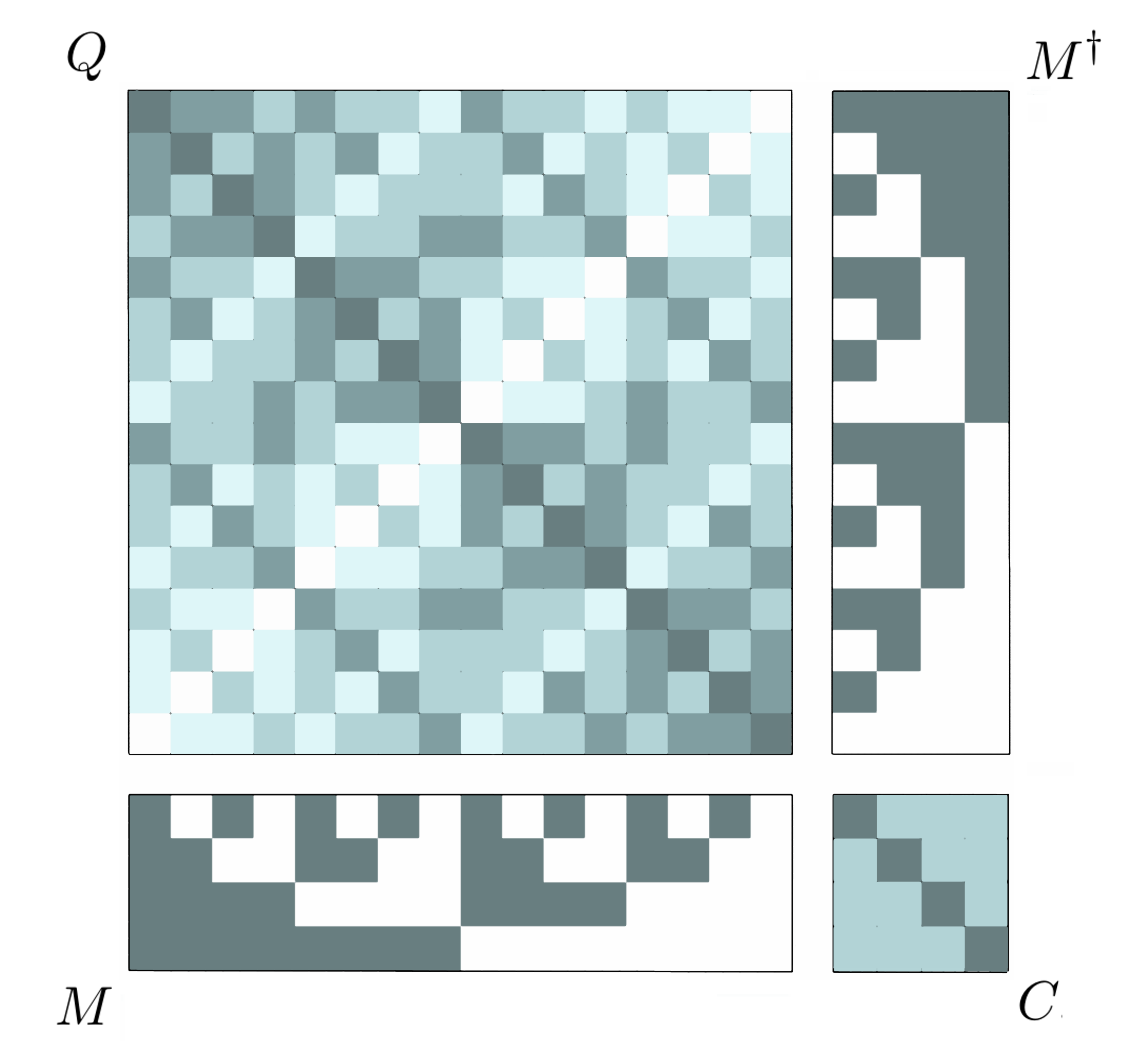
This will be our preferential notation, and we will also use a dedicated symbol for the uniform measure and call it support measure (see upper kernel of Figure 2.1)
| (2.6) |
We can now introduce a powerful graphical tool to represent , that simply consists in rearranging the states into an array. In the following we show how to encode the probability pair into a two dimensional function.
Definition 1.
(Magnetization Kernel) Let , then, the Magnetization Kernel associated to is the step function
| (2.7) |
with indicator function of the event . The sizes of the intervals are
| (2.8) |
An explicit example is given in Figures 2.1 and 2.2, where the states are ordered according to the inverse binary map

Array encodings of the order parameters have been considered since the beginning in the context of the Spin Glasses theory (see the overlap matrix of [2]), but their use to represent probability distributions is recent enough. Before [16, 17], for example, the Aldous-Hoover theorem has been used in [15] to encode the replicated distribution of the SK model into a four dimensional spin tensor. We remark that is defined up to an arbitrary reshuffling of , if we apply the discrete invertible map still
| (2.9) |
because for probability measures the labeling of the support is a free parameter.

Then, the kernel of is not unique, because there are a large number of possible choices for the map that points to the same . But, in general, the order in which the states are observed gives informations about the pattern that minimizes the action. The physical meaning of the index (and the maps in general) is best understood if the same experiment before is figured for spin systems that are not random, for example some Lagrangian system. In this setting two measurements are independent if taken at time intervals that are many times larger than the recurrence time of the system. By choosing a specific order for the states we are then fixing a time gauge, eventually adding some momentum to the Hamiltonian that describes the system.
Notice that the kernel function provides a powerful encoding of correlations and overlaps (and the event algebra in general). The following lemma express this important feature of the kernel representation. Clearly, we can write higher order correlation functions and overlaps using the same procedure:
Definition 2.
(Correlations and Overlaps) Let and select two rows of such that , , then the scalar product between the two rows and is the two point correlation function
| (2.10) |
Moreover, let and be two magnetization states, let and , then the scalar product between the columns and of the kernel is the magnetization overlap between these states
| (2.11) |
The property can be trivially verified by substituting the definition of into the above formulas.
Notice that this last statements admit an interesting operatorial description: if is the transposed kernel, then and , where and are the overlap and correlation matrices rescaled to the unitary square. In fact, according to the Definition 2 we can use kernels to represent creation and annihilation operators by the commutator
| (2.12) |
where and are the overlap and correlation matrices rescaled to the unitary square. Two questions immediately arises, what happen if
| (2.13) |
in some way, and the meaning of the measure associated to .
If the commutator is zero the overlap matrix weakly converges to the correlation matrix, then the averages on matches those on after proper rescaling of the variable on which we take the average. Concerning the transposed measure, it describes a whole new spin system whose correlations and overlaps are exchanged in role respect to , we can give a simple definition as follows:
Definition 3.
(Transposed measure ) Let be a probability measure describing a system of spins, and let be its kernel. Starting from we can define a new sequence of probability measures , each acting on a different spin space with different (eventually much larger) number of spins , such that for the sequence of the associated kernels weakly converges to . We indicate this limit with the symbol , and call it the transposed measure of .
Notice that the sequence is not unique, we can define many that converge to the same limit kernel. To precisely describe these concepts it would be in fact necessary to introduce the cut distance convergence and other graph theoretic arguments that are needed to work with limit kernels (an introduction can be found in Section 3), but there are already interesting cases in which is regular enough such that can be defined also when and are finite. For example, consider the transposed support . Let , and consider the spin vectors
| (2.14) |
then we introduce , that is a collection of states of spins
| (2.15) |
these states are eventually the row vectors of ,
| (2.16) |
and are obtained by the following construction; start from , a magnetization state with all positive spins, and flip half of them to get two groups: one with all positive spins and one with all negative. Then, apply this procedure iteratively inside each group, until the state , where the spins oscillate in sign between each and (see Figure 2.3). Then, the transposed measure is
| (2.17) |
notice that due to their special construction, the states are exactly orthogonal, ie this set has overlap exactly zero between any pair of states.
What allows to define with finite is that the measure is constant, then it can be reduced to a rational number apart from a global rescaling. For non uniform real measures we can only write an approximating sequence: let and split into disjoint regularized subsets with , plus one irregular that collects the real valued reminders:
| (2.18) |
When the reminder becomes irrelevant, and the sequence of measures
| (2.19) |
converges to . Luckily enough, the kernel we will deal with for the SK model (kernel of the eigenstates of magnetization) can be transposed for finite like in the case, and we can partially avoid the technicalities that one would need to manage with limit kernels.
The physical significance of these transposed kernels is in that we interpret them as those that actually describe the 1-RSB phase of the Parisi Ansatz, in fact, we interpret the Parisi full-RSB ansatz as a way to split the systems into sub-systems whose kernel weakly commute in the thermodynamic limit, so that the averages can be done with the transposed measure. We remark that the transposed measure is typically defined on an exponentially larger set of spins: this suggests a connection with the replicated system.
In the Section 4 of this paper, we will show that for SK a possible scheme to obtain such partition into commuting sub-systems is to simply split the spin group into small subgroups and apply the Bayes rule. The physical idea behind is in that any probability measure describing an actual physical spin system defined for variable number of spins must be coherent with the fact that such system has been constructed or created in some way. Then, it must always be possible to construct a sequence of systems of increasing size that eventually converge to the one we are looking at.
Consider, for example, an Ising Model in in which spins are arranged into a cube: such system can be constructed starting with a single spin, then adding a layer of nearest neighbors, then add another and so on, until reaching the size . Notice that this idea is not new at all, being the same that motivates the Cavity methods and the Grand Canonical ensemble.
The most convenient layering scheme depends on the system, but in general each layer has two kinds of energy contributions: those between the spin of the layer itself, that we call the core contribution, and those between the layer and the previous ones (just the previous in case of the finite dimensional Ising model before) that we call the interface.
In the case of fully connected models, we expect that if such partition is into very tiny layers, then the contributions from the core can be ignored respect to that of the interface, and that this will make the layer commute. In fact, notice that in case of the SK model (but the same holds for the Curie-Weiss model) there is no space structure, and any spin that is added form a layer itself, with a large interface. Following [27], we can formally define our analogue of the pure states of the RSB ansatz by partitioning the vertex set into subsets ,
| (2.20) |
we label the parts by the ordered index and also relabel the vertexes inside each , for we apply a map such that . We will refer to
| (2.21) |
as layer magnetization states. Also, it will be convenient to express in terms of the sequence , with and . Starting from this sequence is defined recursively until the last step , corresponding to the whole vertex set. The associated sequence of states is as follows:
| (2.22) |
they are composed by the first sub-states .
Definition 4.
(Filtration of induced by ) Let define the subsets
| (2.23) |
each composed by one element of . Then, the filtration of induced by
| (2.24) |
is defined as the sequence of partitions
| (2.25) |
that is obtained by recursively joining the subsets according to the iteration
| (2.26) |
down to . Let and take some partition , we write
| (2.27) |
for the probability mass of under . Let , then, the average value according to is obtained starting from
| (2.28) |
where , then we iterate the formula backward
| (2.29) |
the average is taken according to the following distribution
| (2.30) |
that is the distribution of the layer for a given [27].
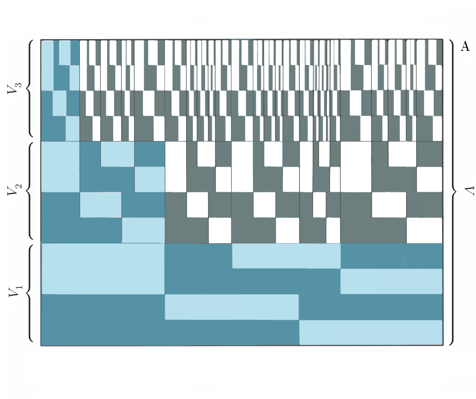
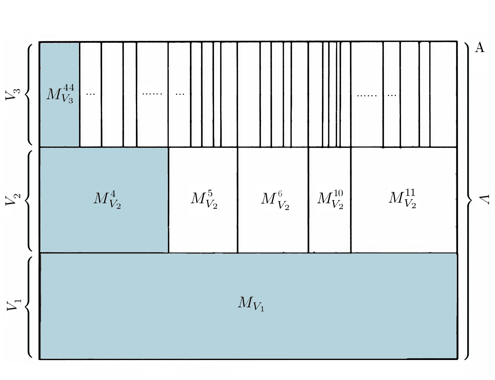
This is enough to analyze the SK Hamiltonian, but before that, it will be useful to discuss the kernel , shown in Figures 2.4, 2.5, 2.6, 2.7. We identify our analogue of the RSB pure states in the sub-kernels associated to the partitions (see below).
We anticipate that the following definition aims to generalize the concept of pure state to any spin distribution, and does not yet have all the properties of the construction that one finds in [20], which we refer to as SK pure states and discuss in Section 4.
Definition 5.
(Analogue Pure States) Let be a filtration induced by the partition as in Definition 4, let be the partition associated to the th level of refinement, and let the kernel associated to . Then, we can identify a partition
| (2.31) |
where is the image of on . Hereafter will refer to these sub-kernels as the Pure States of according to .
The analogue pure states of the -th level are identified with the partition that one gets after refinements of , an example is in Figure 2.5, the sub-kernel associated to the first pure state of each level is highlighted in blue.

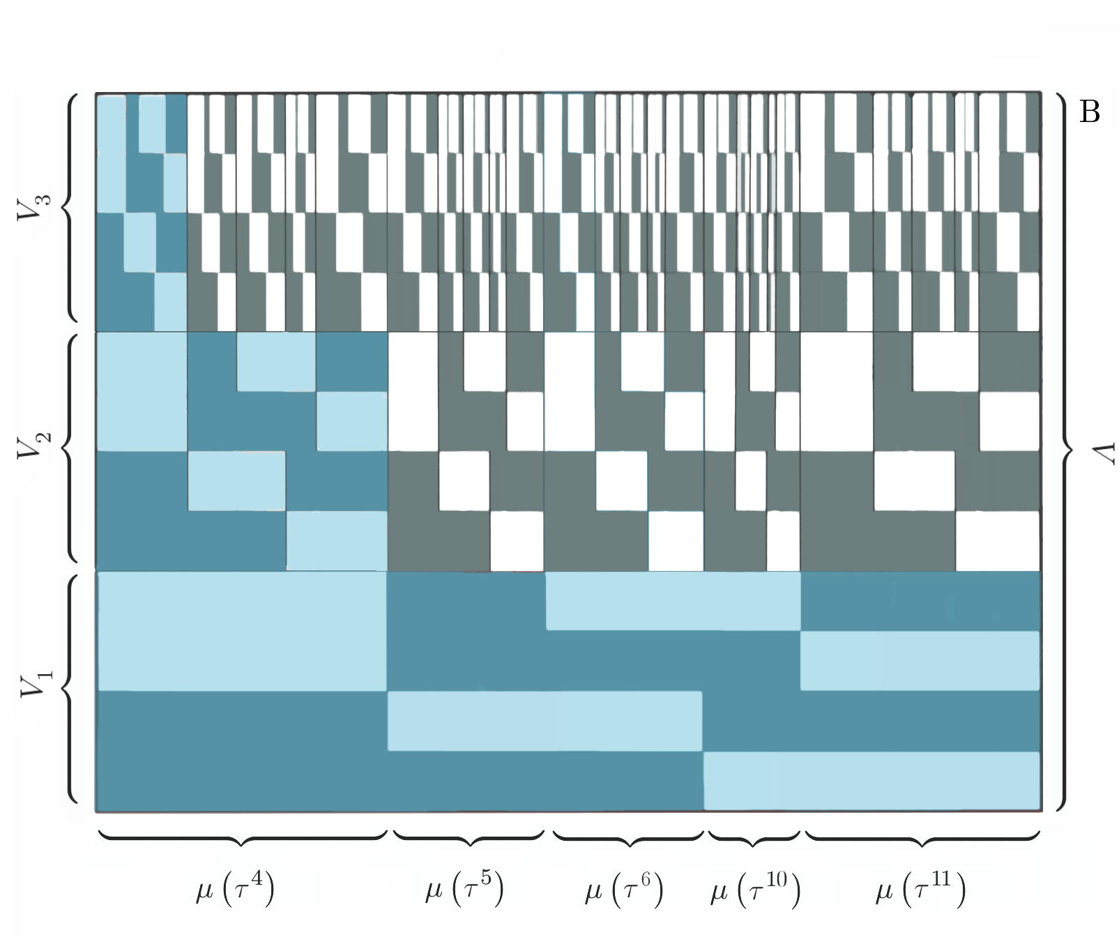

Notice that for any pair of , holds that the overlap (scalar product) between the magnetization states and satisfy the inequality because by definition at least for any . By [20], any overlap distribution inside an SK pure state is expected to concentrate on some nontrivial value for large systems, this is recovered under the additional assumption that and behaves independently for , giving almost surely.
Although the previous definition allows to connect with the usual objects of Spin Glass theory, this partition structure of is not the most natural that one can arrange. In the following we define a second version of the pure states, which we call Layer States. These are not directly related with the usual notion of Pure State that is found in Spin Glass (SG) literature, and we interpret them as the transposed version the 1RSB pure states.
Definition 6.
(Layer states) Let be a filtration induced by the partition as in Definition 4 and let the kernel associated to . We can identify a partition of into the sub-kernels associated to the distributions
| (2.32) |
where and are the images of and on the interval , we will refer to these sub-kernels as the Layer States of according to .
One can confront the kernel of Figure 2.6A with its partition according to the previous definition, Figure 2.7.
The next section contains an introduction to more advanced kernel methods, the reader mostly interested in the physics of the SK model can jump directly to Section 4 for the moment.


3 Kernel filtration
We continue by presenting an alternative approximation scheme that is intended to give a formulation for the finite volume pure states of Marinari et al. in [12] that is also compatible with the kernel methods presented in [16, 17, 18], which allows to operate directly in the thermodynamic limit (TL). In principle, this representation is more general, as it is not based on any special filtration, and in fact contains the one we used for the computations of the SK model as special case. The connection between kernels and the pure states of the RSB ansatz has been first noticed in [16], where a kernel encoding of is introduced in order to prove the following
Lemma.
(Bapst, Coja-Oghlan, 2016) For any measure it is possible to take some arbitrary small and a partition of into a finite number , not dependent from , of disjoint subsets , such that and
| (3.1) |
if is chosen large enough (we denoted by the total variation22 2 Given two measures and some the total variation distance between and is given by the formula .). For example, in the case we can write
| (3.2) |
Proof.
This result tells us that for any measure that describes a system of variables with finite set of inner states we can decompose our sample space into a finite number of regular disjoint subsets , plus one irregular with such that for any regular subset the layers of over a randomly chosen set can be approximated by a product measure in the sense of Eq. (3.1). Surprisingly, the number of such regular subsets only depends on , and the level of precision we want to achieve for our approximation, and it does not depend on the size of the system. This and many other results can be obtained by noticing that both probability measures and graphs can be exactly encoded into kernel functions. For example, in [16, 17, 19] a new distance on based on Graph Theory is introduced to characterize Gibbs Measures directly in the thermodynamic limit.
Definition.
(Cut Distance) Let , be two kernels and let be a pair of measure preserving maps. We call Cut Norm the positive quantity
| (3.3) |
and define the Cut Distance as
| (3.4) |
where stands for [31]. In the context of probability theory the cut distance between is the cut distance between the associated kernels , of Eq.(2.7) below.
It can be shown [31] that the kernel space is compact in the Cut distance, and that convergence in cut distance is stronger than the weak* convergence when dealing with intensive quantities, such as the free energy density associated to a Gibbs measure (see Chapter 8 of [31] and therein, or the first part of [16, 17], see Chapter 8.2 of [31], or [17] for the measure theoretic approach).
The above Lemma is in fact a probabilistic version of the Szemeredi Regularity Lemma (Chapter 9.2 and 9.3 of [31]). Since the arguments presented in the following do not require the use Szemeredi Partitions we won’t discuss this here, but we stress that these are useful mathematical concepts and we warmly advice the reader to look at [29, 31] for further reading on this important subject.
We can give an intuitive picture by considering two independent and equitable partitions of and into sub-sets and , their number being and respectively. Then, define the magnetization averages inside the blocks
| (3.5) |
Then, let and be defined as follows
| (3.6) |
Szemeredi lemma guarantees that, for any small , if and are taken large enough it is possible to find a kernel such that . This fact can already have some interesting applications because the number of parameters that controls the trial measure is finite, although could be very large if we require to be very small. For example, let be some Hamiltonian and the partition function. By definition
| (3.7) |
where in the second row we applied Jensen inequality, and also introduced the Gibbs free energy functional
| (3.8) |
We easily obtained a variational bound for the free energy that is optimized by the Gibbs measure , that is
| (3.9) |
Nonetheless, the function may be hard to handle, because the number of parameters that controls grows exponentially with the size of the system, it is much simpler is to minimize on the parameters that control ,
| (3.10) |
It is possible to show that if the cut distance , then also the free energy densities are weakly convergent.
Definition 7.
(Tree Index for S and V) Let , then, let introduce the following pair of tree indexes. The first is
| (3.11) |
where each subindex runs from to some integer . The second is
| (3.12) |
The integer parameters and are assumed the same for each level . Let define the sets each composed by only one element of mapped onto the Tree Index by the invertible map . Then we call , filtration of , the sequence of equitable refinements
| (3.13) |
obtained from joining the subsets from the last layer down to the root level , associated to . Then, define , containing only one element of mapped on the index by the invertible map . We call filtration of the sequence of refinements of
| (3.14) |
obtained by joining the subsets from the last layer to the root level, associated with itself. We remark that the two filtrations above are defined independently, apart from the fact that must have the same number of levels , the definition of pure state is the same given before in Definition 5, with the refinements on behalf of .
Using both the filtrations and one can construct a sequence of kernels that approximate by progressively averaging (actually “de-averaging”) over the refinements, for example, like in the following nested approximation scheme for the magnetization kernel
Definition 8.
(Magnetization Averages) Start from the last layer , that is associated directly to the external nodes,
| (3.15) |
For all the other layers we define
| (3.16) |
down to the root level , for which we drop the tree index and use simply
| (3.17) |
Starting from the Magnetization Averages we define the parameters
| (3.18) |
that indicate the fluctuation of the magnetization respect to the average of the cell at the level . For the the root level we simply write . In this representation the measure is obtained from the initial condition
| (3.19) |
and then applying the recursive formula
| (3.20) |
to the last level, the measure that we would like to adapt to ,
| (3.21) |
We remark that, by construction, the averages of any respect to the indexes and is zero, and any averaged magnetization can be reconstructed from the increments by summing back them together. The scheme is shown using kernel representation in Figures 3.1 and 3.2.


4 The SK model
We can finally apply these concepts to the SK model. We start introducing the basic quantities of the previous section in the case of Gibbs measures. Consider a system of spins, governed by the Hamiltonian
| (4.1) |
the associated Gibbs measure is
| (4.2) |
the normalization (partition function) is
| (4.3) |
Now, the Hamiltonian of the Sherrington-Kirckpatrick (SK) model [2, 23] is
| (4.4) |
with Gaussian (asymmetric) random matrix with normal independent entries of unitary variance. From now we will work with a random Hamiltonian instead of a single instance of it, so that we don’t have to add another index for the disorder when computing the Gaussian averages (for which we use this special notation). As before, we can define the partition function
| (4.5) |
that in this case is a dependent random quantity.
To simplify some of the coming manipulations we will consider the Asymmetric SK Hamiltonian (ASK),
| (4.6) |
because, apart from vanishing finite size corrections, holds
| (4.7) |
in distribution. Using this definition the temperature is rescaled by a factor respect to the usual Parisi functional. The functional for the original SK model is recovered from that of ASK by substituting with .
Lemma 9.
(Layer States of ASK) Given some partition the ASK Hamiltonian can be decomposed according to Definition 4 as follows
| (4.8) |
where the are the layer Hamiltonians
| (4.9) |
where we introduced the sequence of edges sets
| (4.10) |
In general, we can associate the (random) distributions
| (4.11) |
and the (random) partition functions
| (4.12) |
Proof.
The representation of Definition (4) for ASK is as follows. The partition of is into a number of subsets , each of macroscopic size . As before we write everything in terms of the sets so that all is controlled by the parameters . The sizes of are then . Let
| (4.13) |
be the edges set (for the SK this is a fully connected graph). It is easy to verify that the effect of is to produce a corresponding partition of into subsets such that each contains all edges with both ends in minus those with both ends in (see Figure 4.1). Then we can define a partition of
| (4.14) |
uniquely defined by the partition , the sets are The contribution to the total energy given by is then
| (4.15) |
∎


As said in the previous sections, this partition structure is inspired by the fact that if can be defined for arbitrary sizes then we should be able to represent it as the terminal point of the sequence . Notice that the layer Hamiltonians of Eq.(4.9) can in fact be expressed in terms of the difference between two ASK Hamiltonians, depending on and spins respectively, ie
| (4.16) |
In this form the layer Hamiltonians allow a better reading of what we are actually doing, ie reconstructing the system growing it layer by layer toward a target size . This can be seen also in the Figure 4.1, where a trial partition of the edges set is shown. Here the edges are represented as elements of the square . Remember that the noise of is independent from edge to edge, then also between different . This means that we can average the noise independently for different .
To better understand the physical meaning it will be convenient to introduce the cavity fields that makes the interface
| (4.17) |
with local components given by
| (4.18) |
and same used for the Hamiltonian. Then, the layer can be rewritten as
| (4.19) |
where the self-interaction is simply a smaller ASK Hamiltonian , while the contribution from the interface is mediated by the cavity fields
| (4.20) |
and match the Hamiltonian of an Asymmetric Bipartite SK model (ABSK, see [13]) at slightly shifted temperature, and with ratio between the group sizes that shrinks as increases. Introducing the auxiliary temperature variables
| (4.21) |
we arrive to the expression
| (4.22) |
From this reformulation one can appreciate the structure of the interactions: the cavity fields act as random external fields that depend from the previous level, and toward which the system tries to align, while the thermal fluctuations and the Hamiltonian act as perturbations that can introduce more directions for the eigenstates [27].
Lemma 10.
(IO model) For large and , the Gibbs measure associated to the layer converges in distribution to that of the interface .
Proof.
First we notice that the term is multiplied by and its role become less important as increases. Then, for any finite temperature we can make and large enough to have a sequence for which at any , and it is established since [5] and [6] by second moment methods that in the high temperature regime the annealed averages match the quenched ones. ∎
The layers can be approximated in distribution by the (random) relative weights of the interface only (hereafter IO model),
| (4.23) |
with (random) partition function given by
| (4.24) |
The interface is simply a group of independent spins coupled to a field, that is adapted to the previous layers but does not depend on the one on which acts. To make some stronger statement it will be convenient to introduce the (random) spin vector representing the direction of the external field ,
| (4.25) |
that we call master direction, its components are defined as follows:
| (4.26) |
Notice that due to parity of the function the partition function does not depend on but only on the projections of on the local fields . This vector has all positive entries and can be represented by the Hadamard product between and . Let also introduce the local overlap of the th spin with the direction of the external field
| (4.27) |
this parameter is a measure of how much the spin is binded to the direction of the external field, and depends on the amplitude of .
The parameter is an analogue of the local magnetization, is also related to the local overlap by the formula
| (4.28) |
and can be used as local order parameter. If the amplitude (or ) is large, the spin will be forced to align with the field and . On the contrary, when is small, or is small, then as the spin disentangles from the direction . The fluctuations of the interfaces can be characterized in detail by studying the kernel of Hadamard product between and , the components
| (4.29) |
Notice that the scalar product of spin states (overlap) equals the magnetization of their Hadamard product, also notice that the Hadamard product of a group of spin states by a common master spin state is a theta-map of the kind described in Section 2, and does not change the overlap between the states in the transformed group. Since we are now analyzing the behavior inside a given layer state, we can drop the dependence on previous layers. First notice that the layer Hamiltonian can be written in terms of the vector
| (4.30) |
the relative orientations of and are randomized by the multiplication with the random direction , but are not independent, for example their overlap is the total magnetization of the master direction . Since , for a general non-random function it will be convenient to introduce the associated random function
| (4.31) |
then we can simplify the notation by rewriting as follows
| (4.32) |
and recast the spin variables on which the average is applied:
| (4.33) |
ie, we have changed the sum from to , remembering that the two vectors are uniquely linked and both span the same space.
There is still a little technical difficulty in that are different from site to site. We can overcome this problem in various ways, for example by separating the average from the residual fluctuations of the field:
| (4.34) |
Notice that for the average amplitude converges to a deterministic constant that only depends on the input from the previous layers,
| (4.35) |
where denotes the total magnetization of (that should not be confused with the kernel of the previous sections). As we shall see in short, this expression already allows to establish the connection with the Random Energy Model.
An alternative way is to realize that the layer Hamiltonian is essentially a Number Partitioning Problem (NPP) on the number sequence : the NPR would actually be but the function is the same for both models. Then, following Borgs, Chayes and Pittel [7, 8] (see also [9] for an informal discussion), we reorder the spins of such that the amplitudes form a non-decreasing sequence in , ie such that , this is possible because the fields are extracted independently for different index and there is no space structure to preserve. Then, we can further divide the layers into some large number of sub-layers , of equal volume, marked by : inside these sub-layers the fluctuations are bounded
| (4.36) |
almost everywhere by some constant with finite , so that the fluctuations goes to zero for large and can be neglected. The sub-layers converge to
| (4.37) |
where is the average of inside , then
| (4.38) |
notice that this last representation allows to study the sub-layer in terms of the magnetization eigenstates only, although this is done at the price of introducing a new level of partition.
5 Thermodynamics of the interface
To analyze the sub-layers it will be convenient to further simplify the notation and drop the index for this section. Let the sub-layer measure for some fixed pair and , then, the average of a function can be expressed as:
| (5.1) |
We first do the average according to . Let introduce the set of magnetization eigenstates with given eigenvalue (see Figure 5.1):
| (5.2) |
In what follows it will be convenient to also define a simplified notation , to indicate set of the magnetization eigenstates with given eigenvalue , where is the lower integer part of and .
Lemma 11.
Let be the Gibbs measure associated to the Hamiltonian :
| (5.3) |
the partition function is simply , for large systems the average of some test function respect to converges to
| (5.4) |
the order parameter is the limit magnetization at which the test function is sampled.
Proof.
The set can be studied using Large Deviations Theory (LDT), even at the sample-path LDT level.

For example, following the methods presented in the proof sections of [11], ie by some simple applications of the Varadhan Integral Lemma and other standard LDT theory tools, one can compute and find that is proportional to with convex function of . Given that these methods are well known we only give the essential features.
The average according to can be expressed in terms of the magnetizations eigenstates of as follows:
| (5.5) |
In the last formula we introduced a braket notation for the uniform average on the eigenstates of magnetization: for integer we write
| (5.6) |
that simplifies to in case . In this case is also possible to represent the average in integral form: for any test function
| (5.7) |
The value at which concentrates can be the computed using a saddle point method applied to the pressure functional with entropy functional given by the formula
| (5.8) |
Follows , and . Then we compute the average magnetization by putting the derivative of the pressure to zero, , that is equivalent to impose . In the end one obtains that and finds
| (5.9) |
we remark once again that the average of on the states is taken with equal weights for each magnetization eigenstate. ∎
Then, in the limit of large the sub-layer average is
| (5.10) |
the next lemma we show that at very low temperature the sub-layer fluctuations converge in distribution to the Random Energy Model of Derrida (REM, see also [10, 14, 23] for reviews).
Lemma 12.
(Random Energy Model) Let be some random vector with independent entries of variance as defined in Eq. (4.34), and let be the set of magnetization eigenstates of eigenvalue ,
| (5.11) |
Let be the measure of the generic sub-layer
| (5.12) |
at low temperatures, the fluctuations of the sub-layer converge in distribution to a Random Energy Model.
Proof.
For this proof we assume that the support of is the set of magnetization eigenstates for some given magnetization parameter. Start from
| (5.13) |
and define the following subset of :
| (5.14) |
that contains only those sites of such that is flipped respect to the master direction . Notice that the size of the set is fixed,
| (5.15) |
Further noticing that for the term on the right in Eq. (5.13) holds
| (5.16) |
we can define two new cavity variables, a constant offset
| (5.17) |
and the actual fluctuating term, that is given by
| (5.18) |
then, the fluctuations can be rewritten as
| (5.19) |
the constant offset cancels out in the average formula, and it is possible to rewrite the average in terms of the variables only: we can concentrate on the actually fluctuating component. Notice that by the Central Limit Theorem can be approximated in distribution by a sum of Gaussian variables with variance , ie
| (5.20) |
is approximately a Gaussian variable of unitary variance. Here is the final step: the overlap between the flipped sets and concentrates on in the TL,
| (5.21) |
and vanishes faster than the size of as , then, the fluctuations become asymptotically independent for each input, like in the REM. ∎
Lemma 13.
Let be a positive function of the fluctuations of the cavity fields around the master direction (ground state):
| (5.22) |
defined with an independent noise vector . Then, the average of according to can be approximated by a Poisson Point Process of rate :
| (5.23) |
where is a constant, and and are deterministic parameters that does not depend on the spins of the considered layer (although may still depend from those of the previous).
Proof.
Form the proof of Lemma 12 before, the average formula is
| (5.24) |
and in the low temperature limit we can use the properties of the REM to study it. It is known that for a REM of (random) Gibbs distribution
| (5.25) |
with independent and normally distributed, holds that for any positive test function the (random) average is equal to
| (5.26) |
with rate parameter for , and otherwise.
This result is well known: at low temperatures the weights are proportional in distribution to a Poisson Point Process (PPP) of rate , due to concentration of the measure on the states with lowest energy, and by applying the fundamental averaging property of PPP [14, 23] (see also Little Theorem of [25]) Eq.(5.26) follows. Above the threshold the sampling of the test function is dense and the average is unaffected. We can adapt the formula of Eq. (5.26) to our case using the scaling properties of REM: first rescale the number of spins to take into account the size of : we define with , then rescale the fluctuations of the cavity fields from to spins
| (5.27) |
introducing the modified temperature
| (5.28) |
and substituting in the formula before we arrive to the expression
| (5.29) |
now the REM average formula of Eq. (5.26) can be applied in straight fashion, and we see that, at least in the limit of zero temperature
| (5.30) |
in this limit the rate parameter is given by
| (5.31) |
expanding for we find that near zero temperature
| (5.32) |
It is an interesting fact that the ratio between the original number of spins and the number at which the REM average is computed is exponentially diverging in : this suggests a relation with the transposed measure of Section 2, that can be related to the replicated system, and we interpret as the measure that is actually used in the 1RSB ansatz with replicas. ∎
We have found that, at low temperatures, the layer converges asymptotically to a REM, and can be computed using the properties of PPP. This is not new, in fact, a result similar to Lemma 12 has been obtained for the NPP in [7, 8, 9].
We remark that Eq. (5.30) can be extended to any temperature by noticing that if holds at zero and infinite temperature, then must hold at any intermediate temperature, although with different coefficients. In fact, it is possible to show that for holds
| (5.33) |
due to the fact that the variance of decreases in . Also, when holds , then by Jensen inequality
| (5.34) |
Then, notice that in the high temperature limit obviously holds
| (5.35) |
while from Lemma 13 we have found that
| (5.36) |
Then, in the TL there must be a mapping between and for any , although may be different from that in the proof of Lemma 13 above, that only holds in the low temperature limit.
Lemma 12 completes the mandatory tools to obtain the lower bound of the Parisi formula, using the Cavity Method in the version of [22], but notice that in our reasoning we still did not addressed the distribution of the master direction itself, that is in fact not strictly necessary to compute the free energy by Cavity Method. We propose a conjecture for the full kernel in Figures 5.2 and 5.3 but a detailed argument will be given elsewhere.


6 ROSt variables and Parisi functional
In this end section we will apply our previous findings and methods to the cavity representation of the SK incremental pressure (see for example [22, 23, 27]) and show that by Lemma 12 it can be rewritten to match the functional of the Parisi formula for the SK model (Parisi functional). First, we need to represent the the (random) pressure
| (6.1) |
in terms of some (tractable) functional of , this can be done by cavity method. Following the Random Overlap Structure (ROSt) oriented derivation of [22, 23] we define the ROSt cavity variables, ie the cavity field and the correction term respectively
| (6.2) |
| (6.3) |
the last proportional to the Hamiltonian in distribution. Notice that the above variables are obtained from a noise matrix that is independent from . We keep a tilde on those variables that depends on the new noise.
Apart from vanishing finite size corrections the Cavity representation of the incremental pressure in the version of Aizenmann et al. is [14, 21, 22, 23]
Lemma 14.
Proof.
The result is well known [2] and there are multiple routes, here we follow the derivation that can be found in the last two pages of [21], originally due to Aizenmann et al. [22], see also [14, 23]. The idea is to relate the partition function of an spin system with that of a larger system, then compute the difference between the logarithms of the partition functions. The key ingredient is the Gaussian sum rule
| (6.6) |
where is a new noise matrix independent from the . Applying this to the Hamiltonian gives the following relation that holds in distribution
| (6.7) |
We applied the Gaussian trick before to isolate the correction term, the partition function can be written as
| (6.8) |
Now consider the system of spins, isolating the last spin gives
| (6.9) |
Since the sequence is independent from the other entries, we can write a more pleasant formula by using the diagonal terms of on behalf, ie we take so that the noise relative to the vertex is all expressed in terms of the matrix. The associated partition function is
| (6.10) |
we have written everything in terms of averages respect to a system at slightly shifted temperature. Calling its partition function with
| (6.11) |
and dividing by this quantity both and we arrive to the expression given in the statement by taking , apart from a rescaling of the temperature that becomes negligible in the TL. Notice that since this expression is a representation for the incremental free energy and not the actual free energy, then the proper relation with would be rather
| (6.12) |
but for the SK model it can be shown that the bound is tight [14, 23]. ∎
The cavity formula is then written using Lemma 4 as
| (6.13) |
Here is an important step. Let rewrite the formula once again according to the partition by introducing the variable
| (6.14) |
that is the component of the cavity field normalized by the square root of the number of spins , and the variable
| (6.15) |
that is the component of the correction term, this normalized with the square root of the number of terms contributing to of Lemma 9.
Notice that for fixed both variables are normally distributed. We rewrite the cavity variables in terms of the previous, the first is as follows
| (6.16) |
while for the correction term we can follow the same decomposition presented in Lemma 9 and find
| (6.17) |
where (and not ) comes from removing the constraint under the assumption that is asymmetric almost surely. Recall that by definition the sizes of the sets are
| (6.18) |
| (6.19) |
We can already recognize two familiar coefficients, in particular, these relations allow to identify the sizes of the sets with the overlap parameters as usually intended in the RSB theory. Then, substituting these expressions into the cavity formula before we arrive to
| (6.20) |
As one can easily see, the Definition 4 provides a natural description of the ROSt probability space and its variables. Notice that up to this point all the things that we did on depend on the partition of and hold in general, nonetheless, both the cavity field and the correction term (called fugacity variable in [22]) are now expressed using a common kernel base. In the following theorem, we show how to obtain the functional that appear in the celebrated variational formula by Parisi. Concerning the version of the functional, we refer to the one given in reference [23] for a comparison.
Theorem 15.
Proof.
From Lemma 12 applied to Eq. (6.20) we find
| (6.23) |
in distribution for some constant , and the same can be done for , since in the Eq. (6.23) the uniform average is applied, we can safely take
| (6.24) |
with and independent and normally distributed for all , then
| (6.25) |
and do the same for . Now, start from the initial condition and apply the averages down to . We arrive at
| (6.26) |
Then we can compute the correction term in the same way, finding
| (6.27) |
Putting together, the contributions depending from cancel out,
| (6.28) |
and we obtained the Parisi functional as is presented in [23]. ∎
At this point we can easily understand also the origin of the functional parameters appearing in the Parisi formula. The variables control the energy contributions due to the new spin (actually is the absence of it) and are determined by the relative sizes of the sets in the partition , while the lambda parameters control the cascade of Point Processes.
A fundamental aspect of the Parisi ansatz, which we do not address here, is the special direction of the variational principle to obtain the pressure (one takes the inferior limit of the functional instead of the superior as in Boltzmann theory). Concerning our previous computations, up to now we assumed and fixed to the correct SK value, but one can immediately write the lower bound by varying them
| (6.29) |
Clearly, the hard part is to prove that this inequality is tight. At least for the SK model this has been obtained by proving a matching upper bound via Gaussian interpolation techniques (Guerra-Toninelli interpolation [3]).
Then, the physical meaning of the Parisi variational formula would be in some equilibration condition between the original system and the contributions from the new layer, here composed by just one spin (but one can add more and find the same result). Moreover, it has been proven in [26] that the Parisi functional has a unique minimizer, indicating that such equilibration process has only one result. Since the Parisi principle prescribes to maximize the incremental free energy functional the exact mechanism behind is still not evident, by the way, assuming that the thermodynamic limit exists, then starting from Eq.(6.20) and applying Jensen inequality
| (6.30) |
and since by Eq.(6.28) the functional is distributed like , that is non-random, one finds that is also an upper bound for the expectation of the incremental free energy for any value of and .
7 Conclusions and outlooks
We have described a mathematical formalism that provides a rigorous framework to handle spin glass problems at finite and infinite volume and in a constructive way. In particular, the analogue pure states of Definition 4 allow a constructive approach to the cavity method with ROSt (Sections 4 and 6), and eventually provide a scheme to go from 1RSB to L-RSB once the 1RSB approximation is known. In Section 4 we give a detailed analysis of the martingale representation of [27] and its relation to the Random Energy Model. These manipulations show that a constructive approach to RSB is at least possible without averages and non-standard algebraic tricks.
Concerning the extensibility of the method beyond the SK model, we remark that the arguments of the first three sections and their mathematical formalism are very general, and allow for much in-depth analysis and generalizations. For example, it can be used to deal with any Hamiltonian
| (7.1) |
with being any interaction matrix with fancy underlying topology, and generalized to bipartite and multi-spin interactions by considering higher dimensional kernels (multi-kernels). Also, the kernel formalism allowed to introduce the transposed measure, an interesting probabilistic object that we interpret in the proof of Lemma 13 as physically significant to the replica space.
The arguments of Sections 4, 5 and 6 are also very general, and they can be directly applied for noise that is not Gaussian, and also to the multipartite models. For example, it is possible to repeat the same analysis for the Little model [28], a bipartite system defined by the Hamiltonian
| (7.2) |
We can write the same layer decomposition of Lemma 9, obtaining
| (7.3) |
then we apply Lemma 10, that establish the irrelevance of the energy contribution from the core , and then proceed as in the SK case.
There is a limitation in that Lemma 10 is expected to hold for fully connected models only. In fact, in the case of sparsely connected models the contribution from the layer core to the energy could be still relevant. By the way, detailed computations should be possible for the Bethe Lattice and other sparse but mean-field structured models, in this respect it would be interesting to confront with the loop expansion method of Chertkov, Chernyak, Xiao and Zhou [32].
Concerning finite dimensional lattice models, consider for example the Ising Spin Glass on a dimensional lattice, the Hamiltonian is
| (7.4) |
where is the adjacency matrix of the considered lattice, and
| (7.5) |
are cavity fields that describe the energy contributions from the interface between the spins of and . Then we can apply the layer decomposition to obtain
| (7.6) |
where is the Hamiltonian of the layer’s core, that is a dimensional model. In this case the Lemma 10 cannot be applied, because the core and the interface contributions to the layer energy have comparable sizes, but it should be possible to obtain results with a proper choice of the sequence and the lattice geometry, a short discussion of this can be found in [27].
Although we stop here for this paper, we are persuaded that the kernel framework could provide the ground to systematize many of the known relations between the spin glass problems and other important fields of physics and mathematics, including graph theory [31] (the Section 3 provides the connection with [16, 17, 18, 19] and [31]), neural networks [33, 42] (notice that the structure proposed in Section 4 already resembles a layer neural network), polymers (the layer states of Definition 4 have been used already to compute an urn model approximation of the Range Problem on finite dimensional lattices in [34]) soft granular matter [35], Nelson mechanics [36, 37] (through the commutation properties expressed by Lemma 2), analytic number theory [7, 8, 9, 38, 39, 40] and algorithmic optimization (see [41] for a review). Further investigations will establish where this could eventually bring.
Apart from the spin glass theory and RSB, the kernel representation provides a formal ground to confront datasets from real experiments with kernels from spin glass problems. We remark that datasets of this kind are already available, for example, from neural activity measurements in mammals, most interesting are those from single neuron spike detections (see the kernels obtained in the remarkable experiments of Clawson et al. in [42]).
8 Acknowledgments
I wish to thank Amin Coja-Oghlan (Goethe University, Frankfurt) for explaining the ideas presented in [16], and their connection with Graph Theory and Replica Symmetry Breaking. I also wish to thank Giorgio Parisi, Francesco Guerra, Pietro Caputo, Gioia Pica, Nicola Kistler, Demian Battaglia, Pan Liming, Francesco Concetti and Riccardo Balzan for interesting discussions and suggestions. This project has received funding from the European Research Council (ERC) under the European Union’s Seventh Framework Programme (grant agreement No [278857]) and the European Union’s Horizon 2020 research and innovation programme (grant agreement No [694925]).
References
- [1] G. Parisi, A sequence of approximate solutions to the S-K model for spin glasses, Journal of Physics A 13 (1980) L115.
- [2] G. Parisi, M. Mezard, M. Virasoro, Spin Glass theory and Beyond, World Scientific (1987).
- [3] F. Guerra, Broken replica symmetry bounds in the mean field spin glass model, Communications in Mathematical Physics 233 (2003) 1-12.
- [4] M. Talagrand, The Parisi Formula, Annals of Mathematics 163 (2006) 221-263.
- [5] M. Aizenman, J. L. Lebowitz, D. Ruelle, Some Rigorous Results on the Sherrington-Kirkpatrick Spin Glass Model, Communications in Mathematical Physics 112 (1987) 3-20.
- [6] J. Fröhlich, B. Zegarlinski, Some comments on the Sherrington-Kirkpatrick model of spin glasses, Communications in Mathematical Physics 112 (1987) 553-566.
- [7] C. Borgs, J. Chayes, B. Pittel, Phase transition and finite-size scaling for the integer partitioning problem, Random Structures & Algorithms 34 (2001) 247-288.
- [8] C. Borgs, J. Chayes, S. Mertens, C. Nair, Proof of the local REM conjecture for number partitioning I: Constant energy scales, Random Structures & Algorithms 34 (2009) 217-240.
- [9] H. Bauke, S. Franz, S. Mertens, Number partitioning as random energy model, Journal of Statistical Mechanics: Theory and Experiment P04003 (2004) 217-240.
- [10] A. Bovier, I. Kurkova, Derrida’s Generalised Random Energy models 1: models with finitely many hierarchies, Annales de l’Inistitut Henri Poincaré PR 40 (2004) 439–480.
- [11] S. Franchini, Large deviations for generalized Polya urns with arbitrary urn function, Stochastic Processes and their Applications 127 (10) (2017) 3372-3411.
- [12] E. Marinari, G. Parisi, F. Ricci-Tersenghi, J. Ruiz-Lorenzo, F. Zuliani, Replica Symmetry Breaking in Short-Range Spin Glasses: Theoretical Foundations and Numerical Evidences, Journal of Statistical Physics 98 (2000) 973-1074. Updated 2014 version: https://arxiv.org/abs/cond-mat/9906076
- [13] A. Barra, G. Genovese, F. Guerra, Equilibrium statistical mechanics of bipartite spin systems, Journal of Physics A 44 (2011) 245002.
- [14] D. Panchenko, The Sherrington-Kirckpatrick Model, Springer (2013).
- [15] D. Panchenko, Spin glass models from the point of view of spin distributions, Annals of Probability 41 (2013) 1315-1361.
- [16] V. Bapst, A. Coja-Oghlan, Harnessing the Bethe Free Energy, Random Structures and Algorithms 49 (2016) 694-741.
- [17] A. Coja-Oghlan, W. Perkins, K. Skubch, Limits of discrete distributions and Gibbs measures on random graphs, European Journal of Combinatorics 66 (2017) 37-59.
- [18] A. Coja-Oghlan, W. Perkins, Belief propagation on replica symmetric random factor graph models, Annales de L’Institut Henri Poincare D 5 (2018) 211–249.
- [19] A. Coja-Oghlan, M. Hahn-Klimroth, The Cut Metric for Probability Distributions, SIAM Journal on Discrete Mathematics 35(2) (2021) 1096-1135.
- [20] M. Talagrand, Construction of pure states in mean field models for spin glasses, Probability Theory and Related Fields 148 (2010) 601-643.
- [21] E. Bolthausen, Ultrametricity in Mean-Field Spin Glasses, Asterisque Societé Mathematique de France 367 (2015) 1082.
- [22] M. Aizenmann, R. Sims, S. L. Starr, Mean-field Spin Glass models from the Cavity-ROSt perspective, AMS Contemporary Mathematics Series 437 (2007) 1-30.
- [23] E. Bolthausen, Random Media and Spin Glasses: An Introduction into Some Mathematical Results and Problems, in Spin glasses, Lecture Notes in Mathematics, Springer (2007).
- [24] D. Panchenko, The Parisi Ultrametricity conjecture, Annals of Mathematics 177 (2013) 383-393.
- [25] M. Mézard, G. Parisi, The Bethe lattice spin glass revisited, European Physical Journal B 20 (2001) 217-233.
- [26] A. Auffinger, W.-K. Chen, The Parisi Formula has a unique minimizer, Communications in Mathematical Physics 335 (2015) 1429-1444.
- [27] S. Franchini, A simplified Parisi Ansatz, Communications in Theoretical Physics 73 (2021) 055601.
- [28] R. Brunetti, G. Parisi, F. Ritort, Study of the asymmetric Little model, Physica A: Statistical Mechanics and its Applications Volume 185 (1992) 247-253.
- [29] P. Diaconis, S. Janson, Graph limits and exchangeable random graphs, Rendiconti di Matematica e delle sue Applicazioni VII 28 (2008) 33-61.
- [30] E. Szemerédi, Regular partitions of graphs, Problèmes combinatoires et théorie des graphes, Colloques Internationaux du CNRS 260, Paris (1978) 399–401.
- [31] L. Lovasz, Large Networks and Graph Limits, AMS Colloquim Publications 60 (2012).
- [32] J. Xiao, H. Zhou, Partition function loop series for a general graphical model: free energy corrections and message-passing equations, Journal of Physics A: Mathematical and Theoretical 44 (2011) 425001.
- [33] H. Sompolinsky, A. Crisanti, Chaos in Random Neural Newtorks, Physical Review Letters 61 (1988) 259-262.
- [34] S. Franchini, R. Balzan, Random polymers and generalized urn processes, Physical Review E 98, 042502 (2018) 042502.
- [35] F. P. C. Benetti, G. Parisi, F. Pietracaprina, G. Sicuro, Mean-field model for the density of states of jammed soft spheres, Physical Review E 97 (2018) 062157.
- [36] G. Parisi, Y.-S. Wu, Perturbation theory without gauge fixing, Scientia Sinica 24 (1981) 483.
- [37] E. Brézin, C. Itzykson, G. Parisi, J.-B. Zuber, Planar Diagrams, Communications in Mathematical Physics 59 (1978) 35-51.
- [38] L. P. Arguin, W. Tai, Is the Riemann Zeta Function in a Short Interval a 1-RSB Spin Glass?, Sojourns in Probability Theory and Statistical Physics - I, Springer (2019) 63-88.
- [39] G. Parisi, N. Sourlas, P-adic numbers and replica symmetry breaking, The European Physical Journal B 14 (2000) 535-542.
- [40] V. A. Avetisov, A. H. Bikulov, S. V. Kozyrev, Application of p-adic analysis to models of breaking of replica symmetry, Journal of Physics A 32 (1999) 8785.
- [41] M. Mézard, A. Montanari, Information, Physics, and Computation, Oxford University Press (2009).
- [42] W. Clawson, A. F. Vicente, M. Ferraris, C. Bernard, D. Battaglia, P. P. Quilichini, Computing hubs in the hippocampus and cortex, Science Advances 5 (2019) eaax4843.