Technical Report: Improved Fourier Reconstruction using Jump Information with Applications to MRI
Abstract
Certain applications such as Magnetic Resonance Imaging (MRI) require the reconstruction of functions from Fourier spectral data. When the underlying functions are piecewise-smooth, standard Fourier approximation methods suffer from the Gibbs phenomenon – with associated oscillatory artifacts in the vicinity of edges and an overall reduced order of convergence in the approximation. This paper proposes an edge-augmented Fourier reconstruction procedure which uses only the first few Fourier coefficients of an underlying piecewise-smooth function to accurately estimate jump information and then incorporate it into a Fourier partial sum approximation. We provide both theoretical and empirical results showing the improved accuracy of the proposed method, as well as comparisons demonstrating superior performance over existing state-of-the-art sparse optimization-based methods. Extensions of the proposed techniques to functions of several variables are also addressed preliminarily. All code used to generate the results in this report can be found at [13].
1 Introduction
This paper addresses the problem of reconstructing a -periodic piecewise-smooth function given a small number of its lowest frequency Fourier series coefficients. The Fourier partial sum reconstruction of such piecewise-smooth functions suffers from the Gibbs phenomenon [12] – with its associated non-physical oscillations in the vicinity of jump discontinuities and an overall reduced order of accuracy in the reconstruction. In applications such as MR imaging – where the scanning apparatus collects Fourier coefficients [17] of the specimen being imaged – these oscillatory artifacts and the reduced order of accuracy are significant impediments to generating accurate and fast scan images. Hence, there exists significant ongoing and inter-disciplinary interest in novel methods of reconstructing such functions from Fourier spectral data.
1.1 Related Work
The traditional approach to mitigating Gibbs artifacts is using low-pass filtering [12]. However, this does not completely eliminate all artifacts; filtered reconstructions still suffer from smearing in the vicinity of edges and improved convergence rates are restricted to regions away from edges. Spectral reprojection methods such as [1] work by reconstructing the function in each smooth interval using an alternate (non-periodic) basis such as those consisting of Gegenbauer polynomials. While these methods have been shown to be highly accurate, they are sensitive to parameter choice; indeed, small errors in parameter selection or estimated edge location (which are used to determine the intervals of smoothness) can lead to large reconstruction errors. More recently, there has been significant interest in compressed sensing [4, 5] based approaches to this problem – see, for example, [14, 15]. While these approaches are indeed extremely powerful and versatile, they are implicitly discrete methods and do not perform well when provided with continuous measurements as is the case here. Indeed, we show in the empirical results below that they exhibit poor (first-order) numerical convergence when recovering a piecewise-smooth function from its continuous Fourier measurements. The method proposed in this paper is perhaps most closely related to those in [2, 18, 19, 22, 16, 11, 10] all of which use prony-like methods to estimate the jumps in (after which the jumps’ deleterious spectral effects can be mitigated). In contrast to these previous approaches, however, herein we propose the use of a simple spectral extrapolation scheme together with an alternate (and highly noise robust) non-prony-based jump estimation procedure, provide (-norm) error analysis of the proposed method for general piecewise-smooth functions, present comparisons with state-of-the-art sparse optimization based reconstruction methods, and present preliminary 2D reconstruction results.
The rest of this paper is organized as follows: In §2, we set up notation and provide some definitions before relating jump information to the Fourier coefficients of a piecewise-smooth function. §3 shows how this jump information can be incorporated into a modified Fourier partial sum approximation. Some analytic error bounds for this jump augmented Fourier reconstruction are also provided. Next, §4 defines two different methods of accurately estimating jump information given Fourier spectral data. §5 provides theoretical error bounds for the proposed reconstruction method with estimated edge information while §6 discusses an extension of the method to two-dimensional problems. We provide some concluding comments and directions for future research in §7.
2 Notation, Setup, and Review
We will utilize the following characterization of piecewise smooth functions of one variable.
Definition 2.1.
A -periodic function is piecewise continuous if
- 1.
is Riemann integrable on , and
- 2.
is continuous at all points in except for at most finitely many points
Definition 2.2.
A -periodic function is piecewise smooth if
- 1.
is piecewise continuous,
- 2.
is differentiable on all of , , , , ,
- 3.
as a -periodic function with is also piecewise continuous (having potentially more than discontinuities in ),
- 4.
is differentiable almost everywhere on all of the open intervals between its neighboring discontinuities, and
- 5.
is Lebesgue integrable on .
The Fourier series of a -periodic piecewise smooth function is
where the , the Fourier coefficient of , is
| (1) |
Note that computing the full Fourier series is not always feasible in practice. When this is impossible, a partial Fourier sum
| (2) |
can be used for a given . It is well known that, as increases, converges to pointwise almost everywhere. For example, we have the following theorem.
Theorem 2.1.
(See [7]) If is piecewise smooth then
for every , where and . In particular, for every at which is continuous.
Given that we can expect pointwise convergence of partial Fourier sums as , our next concern becomes determining how large needs to be before we obtain an accurate approximation of . This, in turn, will inevitably lead one to study the decay of as .
2.1 The Fourier Coefficients of Piecewise Smooth Functions with Jumps
Let be a piecewise smooth function with discontinuities (or jumps) at . These -values will also be called jump locations. Considering the Fourier coefficient of ,
and splitting up the integral at the jump locations we can see that
Using integration by parts times we can now see that
Collecting terms, and recalling that is -periodic, we learn that
| (3) |
This brings us to the following useful definition.
Definition 2.3.
The jump function of a piecewise continuous function is defined by
for all . The value will also be referred to as the jump height at .
Through a second use of integration by parts and Definition 2.3 on the integrals (3) we arrive at the following well known result.
Theorem 2.2.
If is piecewise smooth then
holds for all , where is an absolute constant that only depends on and the jump function of . As a result, both and are true.
The relatively slow -decay of the Fourier coefficients of piecewise smooth functions with jumps is closely related to Gibbs phenomenon. In general, the slower decays as , the slower from (2) will converge to as increases (around points of discontinuity in particular).
2.2 Gibbs Phenomenon, and Two Examples
Recall that the Fourier coefficients, , of any piecewise smooth function with jump discontinuities at will exhibit relatively slow -decay (e.g., see Theorem 2.2). Despite this fact, Theorem 2.1 guarantees that for all . However, this convergence of to for almost all is not quite as nice as it looks. It turns out that there exists an absolute constant such that for every one can find many near each jump location with . In short, no matter how large you make , there are guaranteed to be values of near ’s jump locations where approximates badly. This unfortunate fact is known as Gibbs phenomenon.
As an example, let
| (4) |
Note that has six jump discontinuities at , , , , , and . See Figure 1 for its graph.

Another example of a piecewise smooth function with three jump discontinuities is
Note that counts as the third jump location for , with the first two at and . See Figure 2 for its graph.

Gibbs phenomenon implies that functions with multiple jumps, such as in (4), generally require many Fourier coefficients in order to be accurately approximated using standard methods even away from their jumps. As seen in Figures 3 and 5, oscillations around the discontinuities are not reduced as tends to infinity. Furthermore, although the oscillations do decrease away from each jump discontinuity as grows, they decrease rather slowly. In the case of MR imaging, jump discontinuities in the function being measured might, e.g., correspond to tissue boundaries in a patient’s body (e.g., bone to muscle, or from cartilage to fluid). Thus, Gibbs tends to most severely degrade one’s ability to accurately image the boundaries between different tissues. In order to image such regions more accurately, the effects of Gibbs phenomenon must be reduced.



3 A Jump Augmented Partial Sum Reconstruction
Assuming that the jump locations and jump heights of are known, one can use Theorem 2.2 to estimate the Fourier coefficients of for all by
| (5) |
We can now augment (2) by incorporating these jump-based estimates. The resulting augmented partial sum approximation, , is defined by
| (6) |
for all . Note that still only utilizes true Fourier coefficients of .
We would like to use as many terms from the last sum in (6) as we can. Toward this end, let’s consider the form of the complete last sum with . We have that
Note that the Fourier coefficient of the -periodic ramp function , defined by
| (7) |
for all , is given by for all .11 1 See Figure 7 for an example ramp function. Also, .

Thus, we have that
We are now able to give a more easily computable closed for expression for by noting that
| (8) |
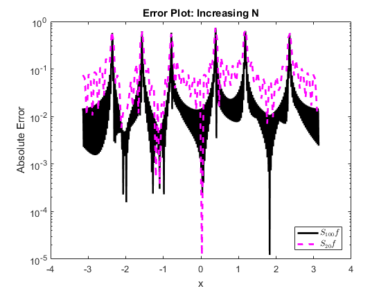
Figure 8 shows this edge-augmented reconstruction using true jump information, , compared to the standard reconstruction, . Notice the great reduction in the Gibbs Phenomenon in the edge-augmented reconstruction. Another feature to take note of is that even thought the standard reconstruction uses more coefficients, the edge-augmented reconstruction is still more accurate (see Figure 10 for an absolute error plot).


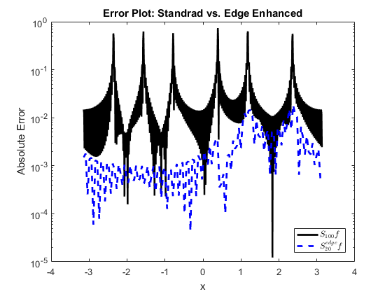
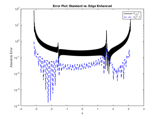
As Figures 10 and 11 demonstrate, the jump-augmented sum is numerically superior to the standard partial sum when it comes to approximating both of our example functions from Section 2.2. In the next subsection we will prove that this is indeed the case more generally.
3.1 Analytical Error Bounds: Jump Information Helps!
We will begin by providing error bounds for in Section 3.1.1. These error bounds are well know – however, we include them here for the sake of completeness. Then, in Section 3.1.2, we will provide error bounds for . As we will see, is guaranteed to converge to in norm much more quickly than does as . In fact, convergence is fast enough that is guaranteed to converge to uniformly as .
3.1.1 Error Bound for
We will begin with a simple theorem that relates the two-norm error to the decay of the Fourier coefficients of .
Theorem 3.1.
Let be a -periodic function with Fourier coefficients satisfying for a given and that are both independent of . Let be the partial Fourier sum approximation of as per (2). Then,
Proof.
We have that
Taking square roots now establishes the desired result. ∎
Theorem 3.1 immediately provides us with the following corollary.
Corollary 3.1.
If is piecewise smooth then
for some constant which is independent of .
The astute reader will be able to see that Corollary 3.1 is actually quite sharp in the case of piecewise smooth functions with jump discontinuities (i.e., there is a similar asymptotic lower bound for with respect to for such functions). Given this, we are now ready to show that converges to in norm faster than does for all piecewise smooth functions with jump discontinuities.
3.1.2 Error Bounds for
Theorem 3.2.
If is piecewise smooth then
for some constant which is independent of .
Proof.
We have that
Taking square roots now yields the desired result. ∎
Similar to Corollary 3.1 above, a very astute reader will be able to see that Theorem 3.2 is sharp with respect to its asymptotic -dependence in the case of piecewise smooth functions that have, e.g., jump discontinuities in their first derivatives. As an example, Figure 12 plots the -error of each reconstruction method for the function from (4) as increases. Notice that the slope for the standard reconstruction error curve, , in Figure 12 is about which is consistent with the exponent on in Corollary 3.1. Similarly, the slope of the jump-augmented reconstruction error curve, , in Figure 12 is about as expected from Theorem 3.2.

The challenge now is that the jump-augmented Fourier sum approximation of , , requires one to know what the true jump heights and jump locations of are. However, this information is often unavailable. When an MRI scan is done, for example, one only has access to a few Fourier coefficients. What is required, then, is a method for finding estimates of a given piecewise smooth function’s jump locations and jump heights, as well as the total number of jumps, that only uses a few Fourier coefficients of the function as input. Two methods that can help us do this are Prony’s Method, and concentration kernels with conjugate sums. Each of these are briefly described in the following section.
4 Numerical Methods for Approximately Computing Using Just a Few Fourier Coefficients
In this section we briefly summarize two different approaches that one can use in order to estimate the jump locations and heights present in a piecewise smooth function using only its first few Fourier series coefficients. We will begin by describing a simple Prony-type method for the problem.
4.1 Prony’s Method
Prony’s method is a technique for transforming a non-linear parameter fitting problem into a sequence of linear and root-finding problems that are easier to solve. Below we will briefly demonstrate how Prony’s Method can be used to estimate the jump heights and jump locations of a piecewise smooth function using only a few of its Fourier coefficients. For a simple introduction to Prony’s method see, e.g., [21, Chapter 2].
Fix a parameter . When given sufficiently many observed values, , Prony’s method solves a system of equations of the form
| (9) |
for the unknowns and , for all . In order to use Prony’s method for our jump height and jump location estimation problem we will make these equations look like the ones approximately provided by Theorem 2.2.
Using Theorem 2.2 and neglecting -terms, we have that
| (10) |
Multiplying through by we can see that
holds for all . Now our unknowns can be renamed to match those of the system that Prony’s method solves (9) as follows: Use the parameter , and let , , and for all . Finally, take our observed values to be
| (11) |
Given this setup a Prony method can now be used in order to estimate all jump locations and jump heights using only the measured Fourier coefficients . See [21, Chapter 2] for details.
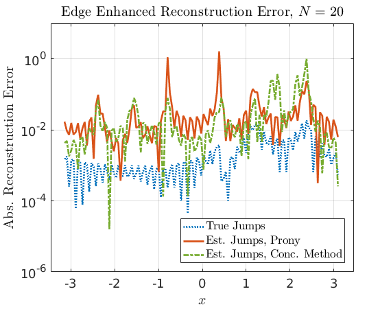
Figure 13 compares the jump-augmented reconstruction method of Section 3 using estimated jump locations and jump heights from Prony’s Method against the same method using true jump information. It performs relatively well despite the small number of Fourier coefficients utilized. See Figure 19 for an absolute error plot. Prony’s method still has some drawbacks, however. For example, it needs to have a relatively accurate estimate for the total number of true jumps, , in order for the method to work well. For this reason, among others, we also looked into the use of concentration kernels and conjugate sums for jump location and height estimation.


4.2 Concentration Kernels
Identifying jump information from spectral data is a challenging task since it involves the extraction of local features from global data. In particular, Fourier reconstructions of piecewise-smooth functions suffer from Gibbs oscillations which can often be mistaken for jumps by conventional edge detectors, such as those based on divided differences. The concentration method of edge detection [8, 9], which was specifically devised to address this problem, computes an approximation to the jump function (Def. 2.3) using a filtered Fourier partial sum of the form
| (12) |
Here, , known as a concentration factor, defines a special class of edge detection “filters”. Under certain admissibility conditions (see [9] for details), the Fourier partial sum (12) “concentrates” at the singular support of and we have the following property ([6, Theorem 2.3]):
where denotes the distance between and the nearest jump discontinuity and depends on the choice of .
| Factor | Expression |
|---|---|
| Trigonometric | |
| Polynomial | |
| is the order of the factor | |
| Exponential | |
| - normalizing constant | |
| - order | |
Some common families of concentration factors and their corresponding plots in Fourier space are provided in Table 1 and Fig. 15 respectively. The jump function approximation produced by each concentration factor is unique and has certain characteristic features. For example, the first order Polynomial concentration factor produces a jump approximation which is equivalent to computing a scaled first derivative of the Fourier partial sum . A jump function approximation using the Trigonometric concentration factor utilizes the approximately Gibbs overshoots and undershoots on either side of a jump to determine both jump locations and heights. Finally, the exponential concentration factor is designed so as to yield root-exponentially small jump approximations away from the jumps.
Once the jump approximation – which can be evaluated efficiently using FFTs – has been computed, the jump locations and values can be identified using simple thresholding and peak finding. This provides estimates of jump locations accurate to the nearest grid point used in the evaluation of the concentration sum (12). However, we note that for well separated jumps (at least away from each other), is a locally convex function and the jump location estimates can be improved by implementing a local gradient-descent based optimization procedure. Alternatively, a non-linear optimization routine (such as one based on the Levenberg-Marquardt algorithm) can be employed in conjunction with Theorem 2.2 to obtain sub-grid accuracy for jump locations and jump values. In Fig. 16(a), a representative jump function approximation using Fourier coefficients of the piecewise-smooth test function (4) and the trigonometric concentration factor is plotted. Matlab’s findpeaks was used to perform peakfinding and the initial jump location estimates were refined using fsolve to implement a non-linear fitting of Theorem 2.2. While we defer analysis of the sub-grid accuracy of the concentration method to future research, we present empirical evidence of this in Figure 16(b), where the error in estimating jump locations and values is plotted as a function of the number of Fourier modes . For reference, results using the Prony procedure from §4.1 – which assumes that the number of jumps is known apriori – is also plotted. The figure shows that both jump locations and values can be estimated at an accuracy even though we are given only Fourier coefficients.
Next, we present numerical results demonstrating robustness of the concentration edge detection method to measurement noise. Fig. 17 plots the error (averaged over trials) in estimating jump information from noise corrupted Fourier coefficients,
where denotes complex Gaussian additive noise of zero mean and variance . The variance is chosen such that
where denotes the vector of true Fourier coefficients. The figure shows that the concentration method is robust to measurement errors; Indeed, at high SNRs (such as in Fig. 17(a)), jump locations are still recovered with accuracy. The figure also shows that the concentration method is much more noise tolerant than the Prony-based method of §4.1. Finally, we note that no specific statistical constructions were used to implement Fig. 17 (such as those in [20]). We leave this to future research where we expect performance improvements.
Figure 18 shows the edge-augmented reconstruction using the concentration jump estimates compared to the reconstruction using true jump information. We see that for very small values of (Fig. 18(a), ), the jump estimates produced by the concentration method are inaccurate leading to errors in the edge-augmented reconstruction. However, for larger values of (Fig. 18(b), ), the edge augmented reconstruction using estimated edge information is comparable to that obtained using true jump information. (See Figure 19 for absolute error plot.)
4.3 Estimate Method Comparison
These methods each have their own strengths and weaknesses. Prony’s Method tends to produce more accurate estimates using less coefficients, but it is highly dependent on the expected number of jumps and is more susceptible to measurement errors. The Concentration Kernel method allows a lot more freedom and possibility for improvement due to our ability to choose sigma, but it does not work as well as prony-type methods when using a very low number of Fourier coefficients. These differences are what make it hard to choose just a single method for obtaining estimated jump information. Most likely a hybrid approach will work the best overall. We suggest the use of Concentration Kernel techniques in the noisy regime where the number of jumps is not known well in advance (but where some additional sampling is possible), and the use of prony-type methods in the low sample, high SNR setting.
5 Error Bounds for the Proposed Numerical Method with Estimated Jump Information
With any method of reconstruction from Section 4 there will be some error involved from the use of estimated jump information (as opposed to true jump information). Our goal is to bound this error and then compare it to the theoretical results in Section 3.1.
Let denote a ramp function with a jump at (7), and let be an associated magnitude (both corresponding to a true jump in a function we seek to approximate). Similarly, let denote another ramp function with a jump at having an associated magnitude of . We will assume in this section that is an approximation of produced by one of the methods in Section 4 from the Fourier coefficients of . These approximate ramp functions are, furthermore, associated with an estimated jump-information based approximation of given by
| (13) |
where denotes the Fourier coefficient of . In this section we seek to better understand the error . Toward that end, we present the following result.
Theorem 5.1.
Let be a piecewise smooth function, be the edge-augmented Fourier sum approximation of with true jump information (8), and be the edge-augmented Fourier sum approximation of with estimated jump information (13). Then, if and both hold for all , we have that
where is a constant which is independent of , , and .
Proof.
We begin with the triangle inequality
Theorem 3.2 can now be applied to bound the first term above. Doing so we learn that
| (14) |
The remainder of the proof is now dedicated to bounding the second term in (14).
Using (6) together with a similar form for we can see that
| (by Parseval’s Theorem) | ||||
| (by Parseval’s Theorem) | ||||
A second use of the triangle inequality now reveals that
| (15) |
Comparing Theorem 5.1 to Corollary 3.1 we can see that from (13) will approximate piecewise smooth functions with jumps better than will as long as is and is . In fact, the numerical behavior is much better than this (suggesting, among other things, that Theorem 5.1 can probably be improved).

Figure 20 shows the error from Figure 12 but now also includes the error from using estimated jump information via Prony’s Method as well as the trigonometric concentration kernel. Once again, the slope of each line in Figure 20 is important to note. Since we won’t have true jump information in applications, we want to see if our estimated information can still give us a similar degree of accuracy as the error expected using true jump information. At lower values of , the error is closer to that of the standard reconstruction, but as increases the slopes of the reconstructions from Prony’s Method and the concentration kernel start to match that of the slope from true jump information. This means the decay for the estimated jump information is a great improvement over the standard reconstruction (and, indeed, near optimal for larger ).
6 Preliminary Two-Dimensional Results
We conclude by presenting preliminary results demonstrating the extension of the proposed method to the two-dimensional case. Consider the reconstruction of a two-dimensional -periodic function given its Fourier series coefficients
| (16) |
If is piecewise-smooth, the 2D Fourier partial sum reconstruction
| (17) |

suffers from Gibbs artifacts as in the one dimensional case. For example, Fig. 21 plots the Fourier partial sum reconstruction of the “box” function
| (18) |
using Fourier series coefficients. Despite the large number of coefficients used in the reconstruction, note the significant Gibbs artifacts along the edges of the function.
To mitigate these artifacts, we consider the following two-dimensional extension of the edge-augmented partial sum procedure of §3. Herein, we use the notation and to denote the row and column cross-sections of respectively. Without loss of generality, and for ease of notation, we assume that . Furthermore, we assume that reconstruction is performed on a equispaced grid in image space.
Two-Dimensional Edge-Augmented Fourier Sum
1Given: Fourier coefficients for
2Define oversampled grid in the -dimension, where
3Reconstruct along the rows of
4
for
5
Approximate Fourier coefficients of the (row) cross-section
.
6
Estimate jump locations and associated jump values
along the cross-section
using §4.1 or §4.2. (Here, denotes the number of
jumps in the cross-section.)
7
Compute the edge-augmented Fourier partial sum approximation of
the (row) cross-section using (13).
8Refine reconstruction along the columns of
9
for
10
Approximate Fourier coefficients of the (column) cross-section using quadrature
.
11
Estimate jump locations and associated jump values
along the cross-section
using §4.1 or §4.2. (Here, denotes the number of
jumps in the cross-section.)
12
Compute edge-augmented Fourier partial sum approximation of
the (column) cross-section using (13).
13
Output the grid values from (column) cross-section estimates as final grid estimates.
Some representative results can be seen in Fig. 22 which plots the reconstruction of the function
(here denotes the indicator function of ) using its two-dimensional (continuous) Fourier series coefficients for . Note that the Fourier coefficients of this function can be evaluated in closed form since the Fourier coefficients of the box and circle are known in closed form. We can see that the standard Fourier partial sum reconstruction in Fig. 22(a) shows significant Gibbs oscillatory artifacts, while the proposed method in Fig. 22(b) is much more accurate. This is especially evident in the error plots of the respective reconstructions – note the large errors along the edges of the features of in the Fourier partial sum, while the edge-augmented reconstruction shows significantly reduced errors and artifacts. Errors are reported in terms of the peak signal to noise ratio (PSNR); let and denote a two-dimensional grid function and its approximation respectively. Then,
As with the one-dimensional case, the concentration kernel edge detection method is used to estimate edge locations and heights from the given Fourier data.


7 Conclusion
In this paper we discuss reconstruction through partial sum approximations and further, seek to reduce the Gibbs phenomenon. We use examples with incorporated true jump information and estimated jump information. We additionally explore two methods (namely, Prony’s Method and the Concentration Kernel Method) to accurately estimate jump heights and locations. We show how these methods can be applied in the one dimensional case while also providing preliminary two dimensional empirical results. Additionally, we derive theoretical error bounds for these methods of reconstruction for the one dimensional case.
There are several avenues for future investigation. First, the noise produced by the MRI machine itself needs to be accounted for in determining the practical robustness of our methods. Second, more advanced Concentration Kernel methods could be developed according to [23] and evaluated against the current results. Similarly, the analytical error bounds and better methods for the two-dimensional case could be developed. See references in, e.g., [3] for more on existing techniques.
8 Acknowledgements
We would like to thank Dr. Tsvetanka Sendova for her insight and guidance throughout this project. We also extend our gratitude to Michigan State University, Lyman Briggs College and, more specifically, Dr. Robert Bell for organizing and hosting the SURIEM (Summer Undergraduate Research Institute in Experimental Mathematics) program this summer. We would also like to thank our home colleges/universities: Wellesley College, Albion College, Goucher College, and the University of Virginia. Lastly, a great thanks to the National Security Agency and National Science Foundation for funding the Mathematics REU.
Project sponsored by the National Science Foundation under Grant Number DMS-1559776.
Project sponsored by the National Security Agency under Grant Number H98230-16-1-0031.
References
- [1] Rick Archibald and Anne Gelb. A method to reduce the Gibbs ringing artifact in MRI scans while keeping tissue boundary integrity. IEEE Trans. Med. Imag., 21(4):305–319, Apr. 2002.
- [2] Dmitry Batenkov. Complete algebraic reconstruction of piecewise-smooth functions from Fourier data. Math. Comp., 84:2329–2350, Feb. 2015.
- [3] Dmitry Batenkov. Complete algebraic reconstruction of piecewise-smooth functions from Fourier data. Math. Comp., 84:2329–2350, 2015.
- [4] Emmanuel J Candes, Justin K Romberg, and Terence Tao. Stable signal recovery from incomplete and inaccurate measurements. Comm. Pure Appl. Math., 59(8):1207–1223, Mar. 2006.
- [5] David L Donoho. Compressed sensing. IEEE Trans. Inf. Theory, 52(4):1289–1306, Apr 2006.
- [6] Shlomo Engelberg and Eitan Tadmor. Recovery of edges from spectral data with noise– a new perspective. SIAM J. Numerical Anal., 46(5):2620–2635, 2008.
- [7] Gerald Folland. Fourier Analysis and its Applications, volume 4. American Mathematical Society, 1992.
- [8] Anne Gelb and Eitan Tadmor. Detection of edges in spectral data. Appl. Comput. Harmonic Anal., 7(1):101–135, 1999.
- [9] Anne Gelb and Eitan Tadmor. Detection of edges in spectral data II. Nonlinear enhancement. SIAM J. Numerical Anal., 38(4):1389–1408, 2000.
- [10] E Mark Haacke, Zhi-Pei Liang, and Steven H Izen. Constrained reconstruction: A superresolution, optimal signal-to-noise alternative to the Fourier transform in magnetic resonance imaging. Med. Phys., 16(3):388–397, 1989.
- [11] E Mark Haacke, Zhi-Pei Liang, and Steven H Izen. Superresolution reconstruction through object modeling and parameter estimation. IEEE Trans. Acoust., Speech, Signal Process., 37(4):592–595, Apr. 1989.
- [12] Jan S. Hesthaven, Sigal Gottlieb, and David Gottlieb. Spectral Methods for Time-Dependent Problems, volume 21 of Cambridge Monographs on Applied and Computational Mathematics. Cambridge University Press, 2007.
- [13] Jade Larriva-Latt et al. FourierRecon: Matlab software for reconstruction from Fourier spectral data. https://www.bitbucket.org/charms/fourierrecon, Sept. 2016.
- [14] Michael Lustig, David Donoho, and John M Pauly. Sparse MRI: The application of compressed sensing for rapid MR imaging. Magn. Reson. Med., 58(6):1182–1195, Dec. 2007.
- [15] Michael Lustig, David L Donoho, Juan M Santos, and John M Pauly. Compressed sensing MRI. IEEE Signal Process. Mag., 25(2):72–82, Mar. 2008.
- [16] Irena Maravic and Martin Vetterli. Sampling and reconstruction of signals with finite rate of innovation in the presence of noise. IEEE Trans. Signal Process., 53(8):2788–2805, 2005.
- [17] Dwight G. Nishimura. Principles of Magnetic Resonance Imaging, chapter Imaging Principles, pages 67–106. Lulu, Raleigh, NC, 1.2 edition, 2010.
- [18] Greg Ongie and Mathews Jacob. Recovery of piecewise smooth images from few fourier samples. In Int. Conf. Sampling Theory and Applications (SampTA), pages 543–547. IEEE, 2015.
- [19] Greg Ongie and Mathews Jacob. Super-resolution MRI using finite rate of innovation curves. In 12th Int. Symp. Biomedical Imaging (ISBI), pages 1248–1251. IEEE, 2015.
- [20] Alex Petersen, Anne Gelb, and Randall Eubank. Hypothesis testing for Fourier based edge detection methods. J. Sci. Comput., 51(3):608–630, 2012.
- [21] Satnam Singh. Application of Prony analysis to characterize pulsed corona reactor measurements. Master’s thesis, University of Wyoming, 2003.
- [22] Martin Vetterli, Pina Marziliano, and Thierry Blu. Sampling signals with finite rate of innovation. IEEE Trans. Signal Process., 50(6):1417–1428, 2002.
- [23] Adityavikram Viswanathan, Anne Gelb, and Douglas Cochran. Iterative design of concentration factors for jump detection. J. Sci. Comput., 51(3):631–649, June 2012.