跳到论文正文
W Papers独立论文阅读器 arXiv:1610.03453 论文正文 计算阅读时间 · 0%
引用这篇论文根据当前论文元数据生成,正式投稿前建议核对。


License: arXiv.org perpetual non-exclusive license
arXiv:1610.03453v2 [hep-ph] 10 Mar 2017

High Energy QCD at NLO: from light-cone wave function to JIMWLK evolution.

Michael Lublinsky Affiliation: Department of Physics, Ben-Gurion University of the Negev, Beer-Sheva 84105, Israel Affiliation: Physics Department, University of Connecticut, 2152 Hillside Road, Storrs, CT 06269-3046, USA Email: lublinm@bgu.ac.il    and Yair Mulian Affiliation: Department of Physics, Ben-Gurion University of the Negev, Beer-Sheva 84105, Israel Email: yair25m@gmail.com
Abstract

Soft components of the light cone wave-function of a fast moving projectile hadron is computed in perturbation theory to the third order in QCD coupling constant. At this order, the Fock space of the soft modes consists of one-gluon, two-gluon, and a quark-antiquark states. The hard component of the wave-function acts as a non-Abelian background field for the soft modes and is represented by a valence charge distribution that accounts for non-linear density effects in the projectile. When scattered off a dense target, the diagonal element of the SS-matrix reveals the Hamiltonian of high energy evolution, the JIMWLK Hamiltonian. This way we provide a new direct derivation of the JIMWLK Hamiltonian at the Next-to-Leading Order.

1 Introduction and Summary

The phenomenon of perturbative saturation is believed to occur in high energy hadronic collisions and is most pronounced in processes involving nuclei. The idea dates back to the seminal paper [1]. It has been long known theoretically [2] that at high energy gluonic density in a hadron grows exponentially. It was suggested in [1] that this growth does not continue indefinitely, but instead the gluon phase space density saturates when it reaches a critical value of order 1/αs1/\alpha_{s}.

In the years since the basic idea has been proposed the theoretical understanding of saturation has progressed significantly [5, 6]. We now have a first principles QCD formulation of high energy evolution, including the saturation effects (see e.g. [3, 4]). The basic framework was derived in [7] – the Balitsky’s hierarchy, and in a series of papers [8] – the Jalilian-Marian, Iancu, McLerran, Weigert, Leonidov, Kovner (JIMWLK) equation or Colour Glass Condensate (CGC).

The JIMWLK Hamiltonian predicts energy evolution of a hadronic observable 𝒪\cal O via functional equation of the form

d​𝒪d​Y=−HJ​I​M​W​L​K​𝒪.\frac{d\cal O}{dY}\,=\,-\,H_{JIMWLK}\,{\cal O}\,. (1.1)

Here the rapidity Y∼ln⁡(e​n​e​r​g​y)Y\sim\ln\,(energy). The JIMWLK Hamiltonian is applicable when one of the colliding particles is dilute (small parton number), such as in forward production in pA collisions at the LHC or in deep inelastic scattering (DIS). While in the dilute-dilute limit, the JIMWLK equation reduces to the linear BFKL equation [2] and its BKP extension [9], it is free from the famous infrared diffusion problem. Furthermore, the major success associated with the JIMWLK is in that it seemingly restores the ss-channel unitarity of scattering amplitudes (see, however, [10] where the ss-channel unitarity of the JIMWLK was argued to be incomplete).

Phenomenology based on complete LO JIMWLK has emerged recently [11, 12, 13, 14] thanks to its reformulation in terms of stochastic Langevin equation [13]. Yet, for most phenomenological applications JIMWLK is commonly replaced by the Balitsky-Kovchegov (BK) equation [7, 15, 16], which is a mean field/large NcN_{c} reduction of the JIMWLK. During the last decade, these developments have become a basis for phenomenological studies of saturation physics applied to high energy/low xx collision data.

HERA has accumulated a vast amount of precise data in the low xx region, which is particularly useful for calibration of gluon distributions used as an input for calculations of less inclusive processes at RHIC and LHC. Several generations of successful saturation-based fits to low xx HERA data are available, from the first work [17], to the latest state of the art AAMQS phenomenology [18]. These provide comprehensive good quality description of the low x data, including the latest available combined H1-ZEUS set [19]. However, HERA was not convincing in experimentally confirming the saturation phenomenon.

Even though the main features of CGC are qualitatively understood, quantitative description is still at an unsatisfactory level as most of the studies have been performed to the lowest order (LO) in αs\alpha_{s}. It is, however, known that higher order corrections could be very significant and their inclusion crucial for qualitatively reliable phenomenology. Calculational control enables to discriminate between different approaches, some of which describe experimental data but do not involve saturation, is critically important and is the main challenge. Precision mandates inclusion of next-to-leading order (NLO) corrections to evolution and improvement of fixed order calculations for a variety of observables.

The era of saturation-based phenomenology with NLO precision just started. Among recent progress in fixed order NLO calculations it is important to mention the virtual photon impact factor computed in [20, 21, 22] and a series of papers on forward particle production in pA collisions [23, 24] (see e.g [25] for a review). The full set of NLO corrections to BK equation was completed in [26] following on the earlier works [27, 28]. When linearised, the NLO BK was shown to coincide with the NLO BFKL computed over a decade earlier [29]. Running coupling effects are known to be phenomenologically important. While they do not account for all the NLO effects in the evolution, they do carry important information about high order corrections. Those were analysed in [27, 30, 31]. Beyond the NLO accuracy, the BFKL was considered in [32, 33].

The NLO extension of the JIMWLK Hamiltonian is imperative for calculation of more general amplitudes, beyond the quark dipole of the BK equation, which determine important experimental observables like single- and double-inclusive particle production. Moreover, precision also mandates going beyond the large NcN_{c} approximation of the BK equation, which is realised by the JIMWLK. The NLO JIMWLK Hamiltonian was obtained in [34, 35, 36] building upon the calculations of [26, 37], and in [38] by a direct calculation extending [26]. A conformal part of the Hamiltonian was also deduced in [39]. The NLO JIMWLK contains information both about the NLO BKP [40, 41] and on αs\alpha_{s} corrections to the triple Pomeron vertex.

While improved equations are known, the key conceptual question remains to be stability of the αs\alpha_{s} expansion. In the framework of the linear BFKL equation the NLO corrections are big [29] and even may lead to negative cross sections. Numerical calculations [42] of forward particle production in pA collisions done in the hybrid formalism of [43] and including NLO corrections [23] displayed similar pathology. The recent study of the NLO BK [44] indicates that the problem is not cured by the non-linear effects. The origin of the problem is understood reasonably well: the LO resummation picks up enhanced logarithmic contributions from the region in the gluon emission phase space, where the underlying approximations break down. These spurious contributions are subtracted in higher orders, thus leading to large negative corrections. To stabilise the expansion, one is normally forced to perform additional collinear resummations introducing kinematical constraints [45, 46, 47, 48, 49] or more involved schemes compatible with the DGLAP equation [50]. It is clear that a good understanding of a systematic approach to rectifying this problem is urgently needed for reliable phenomenological applications of the NLO BK-JIMWLK framework.

In this paper, we report our contribution to the effort in establishing NLO accuracy in saturation physics. Our results are split into two parts. In the first part, the light cone wave function (LCWF) of a fast moving hadron is computed. More precisely, in a typical Born-Oppenheimer approximation, the Hilbert space of a fast moving projectile is split into a “valence” and a “soft” sectors. The valence gluons have longitudinal momenta greater than some ”cutoff" implicitly defined by the collision energy. In the LCWF, these gluons are characterised by correlators of the colour charge densities ρa​(x)\rho^{a}(x) (xx is a transverse coordinate).

Soft gluons with momenta smaller than the cutoff do not participate in scattering. Increasing the energy of the hadron increases longitudinal momenta of the soft gluons and they emerge from below the cutoff. Having done so they contribute to physical observables, such as scattering amplitude, particle production etc. This "soft" component of the LCWF at NLO schematically has the form

|ψ⟩\displaystyle|\psi\rangle =\displaystyle= (1−gs2κ0ρρ−gs4(δ1ρρ+δ2ρρρ+δ3ρρρρ)|nosoftgluons⟩+\displaystyle(1\,-\,g_{s}^{2}\,\kappa_{0}\,\rho\rho\,-\,g_{s}^{4}(\delta_{1}\,\rho\rho\,+\,\delta_{2}\,\rho\rho\rho\,+\,\delta_{3}\,\rho\rho\rho\rho)\,|\,no\,soft\,gluons\rangle+ (1.2)
+\displaystyle+ (gs​κ1​ρ+gs3​ϵ1​ρ+gs3​ϵ2​ρ​ρ+gs3​ϵ3​ρ​ρ​ρ)​|o​n​e​s​o​f​t​g​l​u​o​n⟩\displaystyle(\,g_{s}\kappa_{1}\,\rho\,+\,g_{s}^{3}\epsilon_{1}\,\rho\,+\,g_{s}^{3}\,\epsilon_{2}\,\rho\rho\,+\,g_{s}^{3}\,\epsilon_{3}\,\rho\rho\rho)\,|\,one\,soft\,gluon\rangle
+\displaystyle+ gs2​(ϵ4​ρ+ϵ5​ρ​ρ)​|t​w​o​s​o​f​t​g​l​u​o​n​s⟩+gs2​ϵ6​ρ​|q​u​a​r​k−a​n​t​i​q​u​a​r​k⟩.\displaystyle g_{s}^{2}(\epsilon_{4}\,\rho\,\,+\,\epsilon_{5}\,\rho\rho)\,|\,two\,soft\,gluons\rangle+g_{s}^{2}\,\epsilon_{6}\,\rho\,|\,quark-antiquark\rangle\,.

The coefficient κ1\kappa_{1} is nothing else but the LO Weizsacker Williams gluon emission vertex. Below we compute all the remaining coefficients in the third order perturbation theory in which the valence charges ρa\rho^{a} act as background fields. A major complexity related to this calculation is that these charges are non-commuting operators on the valence Hilbert space forming a local S​U​(Nc)SU(N_{c}) algebra. Neither commute the matrix elements of perturbation operators averaged over the soft states. As a result, we had to rederive the perturbation theory while carefully controlling over the ordering between the matrix elements. Most of the coefficients in the first line in (1.2) are computed from the normalisation of the state. Yet, δ2\delta_{2} turns out to be a tricky one: it vanishes in perturbation theory. In our calculation it emerges as a phase of the wavefunction, which could be determined from a constraint on applicability of the Born-Oppenheimer approximation. This phase is somewhat similar to the Berry phase, though its nature is apparently rooted in the non-commutativity of ρ\rho rather than being sourced by any topology.

While our calculation and presentation of the results below are fully self-contained, admittedly some of them are not new and could be located in the literature. Particularly, the entire quark sector has been worked out in [30] in a formalism that is identical to ours. The coefficients in the second line in (1.2) are related to single inclusive gluon production and we believe that it might be possible to relate ϵ2\epsilon_{2} with partial result of [51]. The comparison is however not straightforward and we have not pursued it. We also believe that some of our results could be extracted from the LCWF of a dense projectile [52], in which αs\alpha_{s} corrections enhanced by the density ρ\rho were resummed.

There are many advantages in having the complete LCWF at NLO. First, it provides an alternative method for derivation of the NLO JIMWLK Hamiltonian. Given the complexity of the latter, it is critical to have an independent cross check of the results before moving forward with any phenomenological applications. This constitutes the second part of our paper. Second, the LCWF formalism is possibly a good starting point to reformulate the NLO JIMWLK as stochastic evolution suitable for numeric simulations. Finally, the formalism makes it possible to simultaneously address NLO corrections to the Hamiltonian and to semi-inclusive observables, such as single inclusive production.

As was mentioned above, with increase of collision energy, the soft modes emerge above the cutoff and contribute to scattering cross sections. Thus they are naturally identified with the source of high energy evolution [53]. Let’s define the projectile averaged S^\hat{S}-matrix

Σ≡⟨ψ|S^− 1|ψ⟩\Sigma\,\equiv\,\langle\psi|\hat{S}\,-\,1|\psi\rangle (1.3)

The averaging is over the soft modes only leaving Σ⁡[ρ]\Sigma[\rho] as operator on the valence Hilbert space. In fact, Σ\Sigma is a rapidity evolution operator

Σ=e−δ​Y​HJ​I​M​W​L​K−1≃−δ​Y​HJ​I​M​W​L​K+12​δ​Y2​HJ​I​M​W​L​K2​…\Sigma\,=\,e^{-\delta Y\,H_{JIMWLK}}\,-1\,\simeq\,-\,\delta Y\,H_{JIMWLK}\,+\,{1\over 2}\,\delta Y^{2}\,H_{JIMWLK}^{2}\,\ldots (1.4)

Here δ​Y\delta Y is a rapidity interval associated with the longitudinal phase space of the soft modes. The JIMWLK Hamiltonian is expandable in αs\alpha_{s}:

HJ​I​M​W​L​K=HJ​I​M​W​L​KL​O​(αs)+HJ​I​M​W​L​KN​L​O​(αs2)+…H_{JIMWLK}\,=\,H^{LO}_{JIMWLK}(\alpha_{s})\,+\,H^{NLO}_{JIMWLK}(\alpha_{s}^{2})\,+\ldots (1.5)

Computing (1.3) with the LCWF (1.2) provides a direct method to determine HJ​I​M​W​L​KN​L​OH^{NLO}_{JIMWLK} defined as

HJ​I​M​W​L​K≡−d​Σd​δ​Y|δ​Y=0H_{JIMWLK}\,\equiv\,-\,{d\Sigma\over d\,\delta Y}\,|_{{\delta Y=0}} (1.6)

This is, however, not how HJ​I​M​W​L​KN​L​OH^{NLO}_{JIMWLK} was obtained in [34, 35, 36]. There, we only assumed the structure (1.2) without computing any of the coefficients. This structure of the LCWF helped us to identify the most general form of HJ​I​M​W​L​KN​L​OH^{NLO}_{JIMWLK}. More constraints on the form of the Hamiltonian came from the symmetries of the theory. As discussed in detail in [54], the theory must have S​UL​(N)×S​UR​(N)SU_{L}(N)\times SU_{R}(N) symmetry, which in QCD terms is the gauge symmetry of |i​n⟩|in\rangle and |o​u​t⟩|out\rangle states and two discrete symmetries: the charge conjugation, and another Z2Z_{2} symmetry, which in [54] was identified with signature, and can be understood as the combination of charge conjugation and time reversal symmetry [55].

The Hamiltonian in [34] was parametrised by five kernels. They were initially fixed by demanding that the evolution equations for the quark dipole and SU(3) baryon generated by this Hamiltonian match the ones known from the literature [26, 37]. The Hamiltonian thus constructed was suitable for evolution of gauge invariant operators only. It was later amended in [36] to also include non-gauge invariant pieces. Interestingly, the terms in the Hamiltonian that originate from the previously discussed δ2\delta_{2} were found in [35] thanks to a constraint on conformal invariance of the JIMWLK Hamiltonian in 𝒩=4{\cal N}=4. We quote these results for the Hamiltonian in Section 2.8. It will become a benchmark for comparison with our direct calculation.

Below we compute (1.3) with the LCWF (1.2). At αs2\alpha_{s}^{2} order, we find terms that are proportional to δ​Y\delta Y and terms that are proportional to δ​Y2\delta Y^{2}. The former are identified with the NLO JIMWLK Hamiltonian (1.6) and we find a complete agreement with our previous results. The latter are naturally identified with (HJ​I​M​W​L​KL​O)2(H^{LO}_{JIMWLK})^{2}, which is a non-trivial cross check on our calculation.

This paper is organised as follows. Section 2 provides an introductory overview of the wavefunctional formalism. We start with presenting the QCD Hamiltonian in the light cone gauge, introduce field quantisation and then discuss the eikonal approximation for the LC Hamiltonian and scattering matrix. To prepare the stage, we derive the LO JIMWLK Hamiltonian and also quote the previous result for the NLO JIMWLK. The LCWF is computed in Section 3. The reader who is interested in the end result only may skip most of the section and proceed directly to the final result summarised in Section 3.5. Section 4 is devoted to the calculation of Σ\Sigma and extraction of the NLO Hamiltonian. Several Appendices contain complementary materials and details of the calculations.

2 Basics of JIMWLK

In this section, we review the main elements of high energy QCD in the light cone Hamiltonian formalism.

2.1 Light Cone QCD Hamiltonian

Our starting point is QCD Hamiltonian in light-cone gauge [56, 57, 58, 59, 60]. In light-cone coordinates, four-vectors are xμ=(x+,x−,𝐱)x^{\mu}=\left(x^{+},\,x^{-},\,\mathbf{x}\right), where x+≡x0+x3x^{+}\,\equiv\,x^{0}\,+\,x^{3} and x−≡x0−x3x^{-}\,\equiv\,x^{0}\,-\,x^{3} stand for longitudinal, while 𝐱=(x1,x2)\mathbf{x}=\left(x_{1},\,x_{2}\right) for transverse components. We adopt mostly negative metric [56]. The light-cone gauge:

Aa+=Aa​0+Aa​3=0.A^{a+}=A^{a0}+A^{a3}=0. (2.7)

Derivation of the Hamiltonian in the light cone gauge can be found in many reviews and original publications. For self-completeness of our presentation the derivation is briefly sketched in Appendix A:

HL​C​Q​C​D=∫d​x−​d2​𝐱​(12​Πa​(x−,𝐱)​Πa​(x−,𝐱)+14​Fi​ja​(x−,𝐱)​Fi​ja​(x−,𝐱)+i​ψ¯​γ+​D+​ψ),\begin{split}&H_{LC\;QCD}\\ &\quad=\int dx^{-}d^{2}\mathbf{x}\left(\frac{1}{2}\Pi^{a}(x^{-},\,\mathbf{x})\,\Pi^{a}(x^{-},\,\mathbf{x})\,+\,\frac{1}{4}F_{ij}^{a}(x^{-},\,\mathbf{x})\,F_{ij}^{a}(x^{-},\,\mathbf{x})\,+\,i\overline{\psi}\gamma^{+}D_{+}\psi\right),\\ \end{split} (2.8)

where the electric and magnetic pieces have the form:

Πa​(x−,𝐱)≡−1∂+​(Dia​b​∂+Aib− 2​g​ψ+†​ta​ψ+),Fi​ja​(x−,𝐱)≡∂iAja−∂iAja−g​fa​b​c​Aib​Ajc.\begin{split}&\Pi^{a}(x^{-},\,\mathbf{x})\,\equiv\,-\,\frac{1}{\partial^{+}}(D_{i}^{ab}\partial^{+}A_{i}^{b}\,-\,2g\psi_{+}^{\dagger}t^{a}\psi_{+}),\\ &F_{ij}^{a}(x^{-},\,\mathbf{x})\,\equiv\,\partial_{i}A_{j}^{a}\,-\,\partial_{i}A_{j}^{a}\,-\,gf^{abc}A_{i}^{b}A_{j}^{c}.\\ \end{split} (2.9)

i∈(1, 2)i\,\in\,(1,\,2) is a transverse component index; ψ\psi denotes Dirac’s 4-component quark spinor11 1 The flavour index is suppressed in this section., while ψ+\psi_{+} is a corresponding 2-component spinor (see Appendix A). After substitution of Πa​(x−,𝐱)\Pi^{a}(x^{-},\,\mathbf{x}) and Fi​ja​(x−,𝐱)F_{ij}^{a}(x^{-},\,\mathbf{x}) in HL​C​Q​C​DH_{LC\;QCD}, the result can be written as HL​C​Q​C​D=H0+Hi​n​tH_{LC\;QCD}=H_{0}+H_{int}, with free Hamiltonian H0H_{0} given by:

H0≡∫d​x−​d2​𝐱​(12​(∂iAja)2+i​ψ+†​∂i∂i∂+​ψ+).\begin{split}&H_{0}\,\equiv\,\int dx^{-}\,d^{2}\mathbf{x}\,\left(\frac{1}{2}(\partial_{i}A_{j}^{a})^{2}\,+\,i\psi_{+}^{\dagger}\frac{\partial_{i}\partial_{i}}{\partial^{+}}\psi_{+}\right).\\ \end{split} (2.10)

The interaction Hamiltonian Hi​n​tH_{int} reads

Hi​n​t\displaystyle H_{int} ≡∫dx−d2𝐱(−gfa​b​cAibAjc∂iAja+g24fa​b​cfa​d​eAibAjcAidAje\displaystyle\equiv\,\int dx^{-}\,d^{2}\mathbf{x}\,\left(-gf^{abc}A_{i}^{b}A_{j}^{c}\partial_{i}A_{j}^{a}\,+\,\frac{g^{2}}{4}f^{abc}f^{ade}A_{i}^{b}A_{j}^{c}A_{i}^{d}A_{j}^{e}\,\right. (2.11)
−g​fa​b​c​(∂iAia)​1∂+​(Ajb​∂+Ajc)+g22​fa​b​c​fa​d​e​1∂+​(Aib​∂+Aic)​1∂+​(Ajd​∂+Aje)\displaystyle-\,gf^{abc}(\partial_{i}A_{i}^{a})\frac{1}{\partial^{+}}(A_{j}^{b}\partial^{+}A_{j}^{c})\,+\,\frac{g^{2}}{2}f^{abc}f^{ade}\frac{1}{\partial^{+}}(A_{i}^{b}\partial^{+}A_{i}^{c})\frac{1}{\partial^{+}}(A_{j}^{d}\partial^{+}A_{j}^{e})
+ 2​g2​fa​b​c​1∂+​(Aib​∂+Aic)​1∂+​(ψ+†​ta​ψ+)+ 2​g2​1∂+​(ψ+†​ta​ψ+)​1∂+​(ψ+†​ta​ψ+)\displaystyle\,+\,2g^{2}f^{abc}\frac{1}{\partial^{+}}(A_{i}^{b}\partial^{+}A_{i}^{c})\frac{1}{\partial^{+}}(\psi_{+}^{\dagger}t^{a}\psi_{+})+\,2g^{2}\frac{1}{\partial^{+}}(\psi_{+}^{\dagger}t^{a}\psi_{+})\frac{1}{\partial^{+}}(\psi_{+}^{\dagger}t^{a}\psi_{+})
− 2g(∂iAia)1∂+(ψ+†taψ+)−gψ+†ta(σi∂i)1∂+(σjAjaψ+)−gψ+†taσiAia1∂+(σj∂jψ+)\displaystyle\,-\,2g(\partial_{i}A_{i}^{a})\frac{1}{\partial^{+}}(\psi_{+}^{\dagger}t^{a}\psi_{+})\,-\,g\psi_{+}^{\dagger}t^{a}(\sigma_{i}\partial_{i})\frac{1}{\partial^{+}}(\sigma_{j}A_{j}^{a}\psi_{+})-\,g\psi_{+}^{\dagger}t^{a}\sigma_{i}A_{i}^{a}\frac{1}{\partial^{+}}(\sigma_{j}\partial_{j}\psi_{+})
OPEN−i​g2​ψ+†​ta​tb​σi​Aia​1∂+​(σj​Ajb​ψ+)).\displaystyle\left.\,-\,ig^{2}\psi_{+}^{\dagger}t^{a}t^{b}\sigma_{i}A_{i}^{a}\frac{1}{\partial^{+}}(\sigma_{j}A_{j}^{b}\psi_{+})\right).

σi\sigma^{i} are Pauli matrices, the matrices tat^{a} denote the S​U​(Nc)SU(N_{c}) gauge group generators in fundamental representation (the gauge group generators in adjoint representation will be denoted by TaT^{a}), which obey the algebra [ta,tb]=i​fa​b​c​tc\left[t^{a},t^{b}\right]=if^{abc}t^{c}, where fa​b​cf^{abc} are structure constants of the gauge group.

2.2 Field Quantisation

Quantisation of the fields is performed in usual manner introducing creation/annihilation operators and imposing commutation (anti-commutation) relations among them. For the gauge fields:

Aia(x)=∫0∞d​k+2​π∫d2​𝐤(2​π)212​k+(aia(k+,𝐤)e−ik⋅x+aia†(k+,𝐤)ei​k⋅x).A_{i}^{a}(x)=\int_{0}^{\infty}\frac{dk^{+}}{2\pi}\int\frac{d^{2}\mathbf{k}}{(2\pi)^{2}}\frac{1}{\sqrt{2k^{+}}}\left(a_{i}^{a}(k^{+},\mathbf{k})e^{-ik\cdot x}+a_{i}^{a\dagger}(k^{+},\mathbf{k})e^{ik\cdot x}\right). (2.12)

The creation and annihilation operators obey the bosonic algebra:

[aia(k+,𝐤),ajb†(p+,𝐩)]=(2π)3δa​bδi​jδ(k+−p+)δ(2)(𝐤−𝐩).\left[a_{i}^{a}(k^{+},\mathbf{k}),\,a_{j}^{b\dagger}(p^{+},\mathbf{p})\right]=(2\pi)^{3}\delta^{ab}\delta_{ij}\delta(k^{+}-p^{+})\delta^{(2)}(\mathbf{k}-\mathbf{p}). (2.13)

Transforming to coordinate space,

aia(k+,𝐤)=∫𝐳e−i𝐤⋅𝐳aia(k+,𝐳),aia†(k+,𝐤)=∫𝐳ei​𝐤⋅𝐳aia†(k+,𝐳),\begin{split}a_{i}^{a}(k^{+},\,\mathbf{k})=\int_{\mathbf{z}}e^{-i\mathbf{k}\cdot\mathbf{z}}\,a_{i}^{a}(k^{+},\,\mathbf{z})\;,\qquad\qquad a_{i}^{a\dagger}(k^{+},\,\mathbf{k})=\int_{\mathbf{z}}e^{i\mathbf{k}\cdot\mathbf{z}}\,a_{i}^{a\dagger}(k^{+},\,\mathbf{z}),\end{split} (2.14)

the commutation relation becomes:

[aia(k+,𝐱),ajb†(p+,𝐲)]=2πδa​bδi​jδ(k+−p+)δ(2)(𝐱−𝐲).\left[a_{i}^{a}(k^{+},\mathbf{x}),\,a_{j}^{b\dagger}(p^{+},\mathbf{y})\right]=2\pi\delta^{ab}\delta_{ij}\delta(k^{+}-p^{+})\delta^{(2)}(\mathbf{x}-\mathbf{y}). (2.15)

For the quark fields:

ψ+α(x)=∑λ=±12χλ∫0∞d​k+2​π∫d2​𝐤(2​π)212(bλα(k+,𝐤)e−ik⋅x+dλα†(k+,𝐤)ei​k⋅x)\psi_{+}^{\alpha}(x)=\sum_{\lambda=\pm\frac{1}{2}}\chi_{\lambda}\int_{0}^{\infty}\frac{dk^{+}}{2\pi}\int\frac{d^{2}\mathbf{k}}{(2\pi)^{2}}\frac{1}{\sqrt{2}}\left(b_{\lambda}^{\alpha}(k^{+},\mathbf{k})e^{-ik\cdot x}+d_{\lambda}^{\alpha\dagger}(k^{+},\mathbf{k})e^{ik\cdot x}\right) (2.16)

The polarisation vectors are:

χ+12=(10),χ−12=(01),\chi_{+\frac{1}{2}}\,=\,\left(\begin{array}[]{c}1\\ 0\end{array}\right),\qquad\quad\chi_{-\frac{1}{2}}\,=\,\left(\begin{array}[]{c}0\\ 1\end{array}\right), (2.17)
χλ1†​I​χλ2=δλ1​λ2,χλ1†​σ3​χλ2= 2​λ1​δλ1​λ2.\chi_{\lambda_{1}}^{\dagger}\,I\,\chi_{\lambda_{2}}\,=\,\delta_{\lambda_{1}\lambda_{2}},\qquad\quad\chi_{\lambda_{1}}^{\dagger}\,\sigma^{3}\,\chi_{\lambda_{2}}\,=\,2\lambda_{1}\delta_{\lambda_{1}\lambda_{2}}. (2.18)

The anti-commutation relations:

{bλ1α(k+,𝐤),bλ2β†(p+,𝐩)}={dλ1α(k+,𝐤),dλ2β†(p+,𝐩)}=(2​π)3​δλ1​λ2​δα​β​δ(2)​(𝐤−𝐩)​δ​(k+−p+).\begin{split}\left\{b_{\lambda_{1}}^{\alpha}(k^{+},\,\mathbf{k}),\,b_{\lambda_{2}}^{\beta\dagger}(p^{+},\,\mathbf{p})\right\}&=\,\left\{d_{\lambda_{1}}^{\alpha}(k^{+},\,\mathbf{k}),\,d_{\lambda_{2}}^{\beta\dagger}(p^{+},\,\mathbf{p})\right\}\\ &=\,(2\pi)^{3}\,\delta_{\lambda_{1}\lambda_{2}}\,\delta^{\alpha\beta}\,\delta^{(2)}(\mathbf{k}-\mathbf{p})\,\delta(k^{+}-p^{+}).\\ \end{split} (2.19)

Transforming the fields to coordinate space a la (2.14):

{bλ1α(k+,𝐱),bλ2β†(p+,𝐲)}={dλ1α(k+,𝐱),dλ2β†(p+,𝐲)}= 2​π​δλ1​λ2​δα​β​δ(2)​(𝐱−𝐲)​δ​(k+−p+).\begin{split}\left\{b_{\lambda_{1}}^{\alpha}(k^{+},\,\mathbf{x}),\,b_{\lambda_{2}}^{\beta\dagger}(p^{+},\,\mathbf{y})\right\}&=\,\left\{d_{\lambda_{1}}^{\alpha}(k^{+},\,\mathbf{x}),\,d_{\lambda_{2}}^{\beta\dagger}(p^{+},\,\mathbf{y})\right\}\,\\ &=\,2\pi\,\delta_{\lambda_{1}\lambda_{2}}\,\delta^{\alpha\beta}\,\delta^{(2)}(\mathbf{x}-\mathbf{y})\,\delta(k^{+}-p^{+}).\end{split} (2.20)

Inserting the field expansions (2.12) and (2.16) into (2.10), the free Hamiltonian becomes:

H0=∫0∞d​k+2​π∫d2​𝐤(2​π)2𝐤22​k+(aia†(k+,𝐤)aia(k+,𝐤)+∑λ[bλα†(k+,𝐤)bλα(k+,𝐤)−dλα(k+,𝐤)dλα†(k+,𝐤)]),\begin{split}H_{0}=\int_{0}^{\infty}\frac{dk^{+}}{2\pi}&\int\frac{d^{2}\mathbf{k}}{(2\pi)^{2}}\frac{\mathbf{k}^{2}}{2k^{+}}\bigg(a_{i}^{a\dagger}(k^{+},\mathbf{k})\,a_{i}^{a}(k^{+},\mathbf{k})\\ &\left.+\sum_{\lambda}\,\left[b_{\lambda}^{\alpha\dagger}(k^{+},\,\mathbf{k})\,b_{\lambda}^{\alpha}(k^{+},\,\mathbf{k})\,-\,d_{\lambda}^{\alpha}(k^{+},\,\mathbf{k})\,d_{\lambda}^{\alpha\dagger}(k^{+},\,\mathbf{k})\right]\right),\\ \end{split} (2.21)

from which the dispersion relation for free quarks and gluons is Ek=𝐤22​k+E_{k}=\frac{\mathbf{k}^{2}}{2k^{+}}. The interacting part of the Hamiltonian will be quantised in subsection 2.5.

2.3 Light Cone Wave-Function of a Fast Hadron

Consider a fast moving projectile hadron at some rapidity Y0Y_{0}. Its LCWF |Ψ⟩𝖸𝟢\left|\Psi\right\rangle_{\mathsf{Y_{0}}} is an eigenfunction of HL​C​Q​C​DH_{LC\,QCD}. It is convenient to split the modes in the LCWF in accord to their longitudinal momenta, introducing a longitudinal cutoff Λ\Lambda, which is implicitly related to the energy of the target hadron (see [61] for review of the formalism). We further assume that the soft modes in the LCWF whose longitudinal momenta k+k^{+} is smaller than Λ\Lambda are not energetic enough to contribute significantly to the scattering process (their contribution is power suppressed by the collision energy). The hard modes with k+>Λk^{+}>\Lambda are also referred as valence modes.

Total energy of the collision can be increased by boosting the projectile: 𝖸=𝖸0+δ​𝖸\mathsf{Y}\,=\,\mathsf{Y}_{0}\,+\,\delta\mathsf{Y}, whereas δ​𝖸\delta\mathsf{Y} is a boost parameter. By boosting the projectile, all the longitudinal momenta of partons in the LCWF get shifted up (Fig.1):

k+⟶eδ​𝖸​k+.k^{+}\;\longrightarrow\;e^{\delta\mathsf{Y}}\,k^{+}. (2.22)

As a result, some of the soft modes that lived below the cutoff Λ\Lambda get lifted above Λ\Lambda and start to contribute to the scattering process. After the boost, these modes occupy a window Λ<k+<Λ​eδ​𝖸\Lambda\,<\,k^{+}\,<\,\Lambda\,e^{\delta\mathsf{Y}}. The valence modes get shifted above this window.

Ignoring the modes below Λ\Lambda, the LCWF |Ψ⟩𝖸𝟢\left|\Psi\right\rangle_{\mathsf{Y_{0}}} before the boost is dominated by the valence modes only, whose distribution is approximately independent of their longitudinal momenta.

|Ψ⟩𝖸𝟢=|υ⟩.\left|\Psi\right\rangle_{\mathsf{Y_{0}}}\,=\,\left|\upsilon\right\rangle. (2.23)

Here |v⟩|v\rangle represents a valence state with no soft gluons (vaccuum of soft gluons). We assume that this LCWF is known. The LCWF after the boost is

|Ψ⟩𝖸=|ψ⟩⊗|υ⟩,\left|\Psi\right\rangle_{\mathsf{Y}}\,=\,\left|\psi\right\rangle\,\otimes\,\left|\upsilon\right\rangle, (2.24)

where |ψ⟩\left|\psi\right\rangle denotes the soft part of the wave function living in the window Λ<k+<Λ​eδ​𝖸\Lambda\,<\,k^{+}\,<\,\Lambda\,e^{\delta\mathsf{Y}}. The factorisation (2.24) is a typical Born-Oppenheimer approximation. Our goal below will be to find |ψ⟩\left|\psi\right\rangle by perturbatively diagonalising HL​C​Q​C​DH_{LC\,QCD} on the Hilbert space of the soft modes, assuming the valence sector is known and frozen.

Refer to caption
Figure 1: The LCWFs before and after boost. Here ρ\rho stands for the colour charge density of the valence modes, and A for the soft gluon field.

2.4 Eigenstates of Free Hamiltonian

We denote by |0⟩\left|0\right\rangle the vacuum state of the free Hamiltonian H0H_{0} on the soft Hilbert space. The energy of this state will be set to zero, E0=0E_{0}=0. The vacuum is defined as:

aia(k+,𝐤)|0⟩=0,biα(k+,𝐤)|0⟩=0,diα(k+,𝐤)|0⟩=0,a_{i}^{a}(k^{+},\,\mathbf{k})\left|0\right\rangle=0,\qquad\qquad b_{i}^{\alpha}(k^{+},\,\mathbf{k})\left|0\right\rangle=0,\qquad\qquad d_{i}^{\alpha}(k^{+},\,\mathbf{k})\left|0\right\rangle=0, (2.25)

for any Λ<k+<eδ​𝖸​Λ\Lambda<k^{+}<e^{\delta\mathsf{Y}}\Lambda. The soft vacuum |0⟩\left|0\right\rangle should be understood as |0⟩⊗|v⟩\left|0\right\rangle\otimes|v\rangle and, because of its valence component, it differs from the QCD vacuum. As explained above, our prime objective in the next section will be to develop a perturbation theory for this soft vacuum state. Three eigenstates of H0H_{0} will emerge in the NLO calculation below:
∙\bullet One gluon state:

|gia(k)⟩≡aia†(k)(2​π)3/2|0⟩or|gia(k+,𝐳)⟩≡aia†(k+,𝐳)(2​π)1/2|0⟩,\left|g_{i}^{a}(k)\right\rangle\,\equiv\,\frac{a_{i}^{a\dagger}(k)}{(2\pi)^{3/2}}\left|0\right\rangle\qquad or\qquad\left|g_{i}^{a}(k^{+},\,\mathbf{z})\right\rangle\,\equiv\,\frac{a_{i}^{a\dagger}(k^{+},\,\mathbf{z})}{(2\pi)^{1/2}}\left|0\right\rangle, (2.26)

These is a normalised state with the normalisation

⟨gjb(p)|gia(k)⟩=δa​bδi​jδ(2)(𝐤−𝐩)δ(k+−p+)\left\langle g_{j}^{b}(p)\left|g_{i}^{a}(k)\right.\right\rangle=\delta^{ab}\delta_{ij}\delta^{(2)}(\mathbf{k}-\mathbf{p})\delta(k^{+}-p^{+})\;

and

⟨gjb(p+,𝐳′)|gia(k+,𝐳)⟩=δa​bδi​jδ(2)(𝐳−𝐳′)δ(k+−p+).\;\left\langle g_{j}^{b}(p^{+},\,\mathbf{z}^{\prime})\left|g_{i}^{a}(k^{+},\,\mathbf{z})\right.\right\rangle\,=\,\delta^{ab}\,\delta_{ij}\,\delta^{(2)}(\mathbf{z}-\mathbf{z}^{\prime})\,\delta(k^{+}-p^{+}).

This state has the energy Eg​(k)=𝐤22​k+.E_{g}(k)=\frac{\mathbf{k}^{2}}{2k^{+}}.
∙\bullet Two gluon state:

|gia(k)gjb(p)⟩≡aia†(k)ajb†(p)(2​π)3|0⟩or|gia(k+,𝐳)gjb(p+,𝐳′)⟩≡aia†(k+,𝐳)ajb†(p+,𝐳′)2​π|0⟩.\begin{split}&\left|g_{i}^{a}(k)\,g_{j}^{b}(p)\right\rangle\,\equiv\,\frac{a_{i}^{a\dagger}(k)\,a_{j}^{b\dagger}(p)}{(2\pi)^{3}}\left|0\right\rangle\qquad or\\ &\left|g_{i}^{a}(k^{+},\,\mathbf{z})\,g_{j}^{b}(p^{+},\,\mathbf{z}^{\prime})\right\rangle\,\equiv\,\frac{a_{i}^{a\dagger}(k^{+},\,\mathbf{z})\,a_{j}^{b\dagger}(p^{+},\,\mathbf{z}^{\prime})}{2\pi}\left|0\right\rangle.\\ \end{split} (2.27)

with the energy Eg​g​(k,p)≡𝐤22​k++𝐩22​p+E_{gg}(k,\,p)\,\equiv\,\frac{\mathbf{k}^{2}}{2k^{+}}+\frac{\mathbf{p}^{2}}{2p^{+}}.
∙\bullet Quark anti-quark state:

|q¯λ2β(p)qλ1α(k)⟩≡bλ1α†(k)dλ2β†(p)(2​π)3|0⟩or|q¯λ2β(p+,𝐳′)qλ1α(k+,𝐳)⟩≡bλ1α†(k+,𝐳)dλ2β†(p+,𝐳′)2​π|0⟩,\begin{split}&\left|\bar{q}_{\lambda_{2}}^{\beta}(p)\,q_{\lambda_{1}}^{\alpha}(k)\right\rangle\,\equiv\,\frac{b_{\lambda_{1}}^{\alpha\dagger}(k)\,d_{\lambda_{2}}^{\beta\dagger}(p)}{(2\pi)^{3}}\left|0\right\rangle\quad\;or\\ &\left|\bar{q}_{\lambda_{2}}^{\beta}(p^{+},\,\mathbf{z}^{\prime})\,q_{\lambda_{1}}^{\alpha}(k^{+},\,\mathbf{z})\right\rangle\,\equiv\,\frac{b_{\lambda_{1}}^{\alpha\dagger}(k^{+},\,\mathbf{z})\,d_{\lambda_{2}}^{\beta\dagger}(p^{+},\,\mathbf{z}^{\prime})}{2\pi}\left|0\right\rangle,\\ \end{split} (2.28)

with the energy Eq​q¯​(k,p)=𝐤22​k++𝐩22​p+E_{q\bar{q}}(k,\,p)=\frac{\mathbf{k}^{2}}{2k^{+}}+\frac{\mathbf{p}^{2}}{2p^{+}}.

2.5 Eikonal Approximation for QCD Hamiltonian

In section 2.3, we split the Hilbert space into soft and valence modes and introduced a Born-Oppenheimer approximation for the LCWF. Accordingly, we have to split the Hamiltonian Hi​n​tH_{int} as defined by (2.11) into "soft" and "valence". First, we introduce field decomposition: Aia​(x)=A¯ia​(x)+A¯ia​(x)A_{i}^{a}(x)=\underline{A}_{i}^{a}(x)+\overline{A}_{i}^{a}(x) and ψ+α​(x)=ψ¯+α​(x)+ψ¯+α​(x)\psi_{+}^{\alpha}(x)=\underline{\psi}_{+}^{\alpha}(x)+\overline{\psi}_{+}^{\alpha}(x) where the underlined fields contain only modes with longitudinal momenta in the interval k+∈(Λ,eδ​𝖸​Λ)k^{+}\in\left(\Lambda,\,e^{\delta\mathsf{Y}}\Lambda\right) (soft modes) while the fields with the bar contain modes with k+>eδ​𝖸​Λk^{+}>e^{\delta\mathsf{Y}}\Lambda (valence modes). Substitution of this decomposition into Hi​n​tH_{int} is done in Appendix B.

Our next step is to introduce an eikonal approximation for the interaction Hamiltonian. A typical longitudinal momentum of a valence mode is much larger than that of a soft mode. Consequently, all the terms in Hi​n​tH_{int} that are suppressed by the ratio of soft to valence longitudinal momenta can be systematically ignored. Keeping these terms would introduce non-eikonal power suppressed corrections to our calculation. Example of terms in the Hamiltonian which are neglected 1∂+​(A¯jb​∂+A¯jc)\frac{1}{\partial^{+}}(\underline{A}_{j}^{b}\partial^{+}\overline{A}_{j}^{c}) or 1∂+​(ψ¯+†​ta​ψ¯+)\frac{1}{\partial^{+}}(\underline{\psi}_{+}^{\dagger}t^{a}\overline{\psi}_{+}). The action of 1∂+\frac{1}{\partial^{+}} is equivalent to division by a very large valence momentum (i.e. 1p+→0\frac{1}{p^{+}}\rightarrow 0 for any p+>eδ​𝖸​Λp^{+}>e^{\delta\mathsf{Y}}\Lambda).

In Appendix B, we first split the modes between soft and valence in Hi​n​tH_{int} and then employ the eikonal approximation. The result is

Hi​n​t=Hg+Hg​q​q+Hg​g​g+Hg​g​g​g+Hg​g​q​q+Hq​q−i​n​s​t+Hg​g−i​n​s​t+Hg​q+HV.H_{int}=H_{g}+H_{gqq}+H_{ggg}+H_{gggg}+H_{ggqq}+H_{qq-inst}+H_{gg-inst}+H_{gq}+H_{V}. (2.29)

The first eight contributions defined by (B.281) −- (B.288), account for soft-soft and soft-valence interactions, while HVH_{V} involves valence-valence interactions only.

Here ρa​(−𝐩)\rho^{a}(-\mathbf{p}) denotes the total valence current (charge density operator) which acts as a background for the soft fields, and is defined by:

ρa​(−𝐩)≡ρga​(−𝐩)+ρq​q¯a​(−𝐩),\begin{split}\rho^{a}(-\mathbf{p})\,\equiv\,\rho_{g}^{a}(-\mathbf{p})+\rho_{q\bar{q}}^{a}(-\mathbf{p}),\end{split} (2.30)

with

ρga(−𝐩)≡−ifa​b​c∫eδ​𝖸​Λ∞d​k+2​π∫d2​𝐤(2​π)2aj†b(k+,𝐤)ajc(k+,𝐤+𝐩),\begin{split}\rho_{g}^{a}(-\mathbf{p})\,\equiv\,-if^{abc}\int_{e^{\delta\mathsf{Y}}\Lambda}^{\infty}\frac{dk^{+}}{2\pi}\int\frac{d^{2}\mathbf{k}}{(2\pi)^{2}}\,a_{j}^{\dagger b}(k^{+},\,\mathbf{k})\,a_{j}^{c}(k^{+},\,\mathbf{k}+\mathbf{p}),\end{split} (2.31)

and

ρq​q¯a(−𝐩)≡tα​βa∫eδ​𝖸​Λ∞d​k+2​π∫d2​𝐤(2​π)2(bλα†(k+,𝐤−𝐩)bλβ(k+,𝐤)+dλβ(k+,𝐤)dλα†(k+,𝐤−𝐩)).\rho_{q\bar{q}}^{a}(-\mathbf{p})\,\equiv\,t_{\alpha\beta}^{a}\int_{e^{\delta\mathsf{Y}}\Lambda}^{\infty}\frac{dk^{+}}{2\pi}\int\frac{d^{2}\mathbf{k}}{(2\pi)^{2}}\,\left(b_{\lambda}^{\alpha\dagger}(k^{+},\,\mathbf{k}-\mathbf{p})\,b_{\lambda}^{\beta}(k^{+},\,\mathbf{k})+d_{\lambda}^{\beta}(k^{+},\,\mathbf{k})\,d_{\lambda}^{\alpha\dagger}(k^{+},\,\mathbf{k}-\mathbf{p})\right). (2.32)

The valence current ρa​(𝐩)\rho^{a}(\mathbf{p}) satisfies the S​U​(Nc)SU(N_{c}) algebra:

[ρa(𝐱),ρb(𝐲)]=ifa​b​cρc(𝐱)δ(2)(𝐱−𝐲);[ρa(𝐤),ρb(𝐩)]=ifa​b​cρc(𝐤+𝐩).\begin{split}\left[\rho^{a}(\mathbf{x}),\,\rho^{b}(\mathbf{y})\right]=if^{abc}\rho^{c}(\mathbf{x})\delta^{(2)}(\mathbf{x}-\mathbf{y})\>;\quad\quad\left[\rho^{a}(\mathbf{k})\,,\,\,\rho^{b}(\mathbf{p})\right]=if^{abc}\rho^{c}(\mathbf{k}+\mathbf{p})\>.\end{split} (2.33)

where ρa​(𝐱)\rho^{a}(\mathbf{x}) is a Fourier transform of ρa​(𝐩)\rho^{a}(\mathbf{p}):

ρa(𝐱)=1(2​π)2∫d2𝐤ei​𝐤⋅𝐱ρa(−𝐤);ρa(−𝐤)=∫d2𝐱e−i𝐤⋅𝐱ρa(𝐱).\begin{split}&\rho^{a}(\mathbf{x})=\frac{1}{(2\pi)^{2}}\int d^{2}\mathbf{k}\,e^{i\mathbf{k}\cdot\mathbf{x}}\rho^{a}(-\mathbf{k})\;;\qquad\qquad\rho^{a}(-\mathbf{k})=\int d^{2}\mathbf{x}\,e^{-i\mathbf{k}\cdot\mathbf{x}}\rho^{a}(\mathbf{x})\>.\end{split} (2.34)

As a preparation for the next section, it is useful to express (B.281) −- (B.285) in terms of the creation and annihilation operators. This is done by employing the expansions (2.12) and (2.16). Only the terms, which would yield a non-trivial contribution when inserted between the three states defined in section 2.3, and the soft vacuum, will be kept. We omit further details and write the final results,

𝖧g=∫Λeδ​𝖸​Λd​k+2​π∫d2​𝐤(2​π)2g​𝐤i2​|k+|3/2[aia†(k+,𝐤)ρa(−𝐤)+aia(k+,𝐤)ρa(𝐤)],\mathsf{H}_{g}=\int_{\Lambda}^{e^{\delta\mathsf{Y}}\Lambda}\frac{dk^{+}}{2\pi}\int\frac{d^{2}\mathbf{k}}{(2\pi)^{2}}\frac{g\mathbf{k}^{i}}{\sqrt{2}|k^{+}|^{3/2}}\left[a_{i}^{a\dagger}(k^{+},\,\mathbf{k})\rho^{a}(-\mathbf{k})+a_{i}^{a}(k^{+},\,\mathbf{k})\rho^{a}(\mathbf{k})\right], (2.35)
𝖧g​q​q\displaystyle\mathsf{H}_{g\>qq} =∑λ1,λ2=±12∫Λeδ​𝖸​Λd​k+2​π​d​p+2​π​d​q+​∫d2​𝐤(2​π)2​d2​𝐩(2​π)2​d2​𝐪​g​tα​βa2​2​k+​δ(3)​(k−p−q)​Γλ1​λ2i\displaystyle=\sum_{\lambda_{1},\,\lambda_{2}=\pm\frac{1}{2}}\int_{\Lambda}^{e^{\delta\mathsf{Y}}\Lambda}\frac{dk^{+}}{2\pi}\frac{dp^{+}}{2\pi}dq^{+}\,\int\frac{d^{2}\mathbf{k}}{(2\pi)^{2}}\frac{d^{2}\mathbf{p}}{(2\pi)^{2}}d^{2}\mathbf{q}\,\frac{gt_{\alpha\beta}^{a}}{2\sqrt{2k^{+}}}\,\delta^{(3)}(k-p-q)\,\Gamma_{\lambda_{1}\lambda_{2}}^{i} (2.36)
×(aia(k+,𝐤)bλ1α†(p+,𝐩)dλ2β†(q+,𝐪)+h.c.),\displaystyle\times\,(a_{i}^{a}(k^{+},\,\mathbf{k})\,b_{\lambda_{1}}^{\alpha\dagger}(p^{+},\,\mathbf{p})\,d_{\lambda_{2}}^{\beta\dagger}(q^{+},\,\mathbf{q})\,+\,h.c.),

with

Γλ1​λ2i=χλ1†​[2​𝐤ik+−σ⋅𝐩p+​σi−σi​σ⋅𝐪q+]​χλ2,\Gamma_{\lambda_{1}\lambda_{2}}^{i}=\chi_{\lambda_{1}}^{\dagger}\left[\frac{2\mathbf{k}^{i}}{k^{+}}-\frac{\sigma\cdot\mathbf{p}}{p^{+}}\sigma^{i}-\sigma^{i}\frac{\sigma\cdot\mathbf{q}}{q^{+}}\right]\chi_{\lambda_{2}}, (2.37)
𝖧g​g​g=−∫Λeδ​𝖸​Λd​k+2​πd​p+2​πdq+∫d2​𝐤(2​π)2d2​𝐩(2​π)2d2𝐪i​g​fa​b​c2​2​k+​p+​q+×[(𝐪i−q+p++q+𝐤i)aia(k)ajb†(p)ajc†(q)δ(3)(−k+p+q)+(𝐪i+p++q+q+−p+𝐤i)aia†(k)ajb†(p)ajc(q)δ(3)(k+p−q),+h.c.]\begin{split}\mathsf{H}_{g\>gg}=&-\int_{\Lambda}^{e^{\delta\mathsf{Y}}\Lambda}\frac{dk^{+}}{2\pi}\,\frac{dp^{+}}{2\pi}\,dq^{+}\,\int\frac{d^{2}\mathbf{k}}{(2\pi)^{2}}\,\frac{d^{2}\mathbf{p}}{(2\pi)^{2}}\,d^{2}\mathbf{q}\,\frac{igf^{abc}}{2\sqrt{2k^{+}p^{+}q^{+}}}\\ &\times\left[\left(\mathbf{q}^{i}-\frac{q^{+}}{p^{+}+q^{+}}\mathbf{k}^{i}\right)a_{i}^{a}(k)a_{j}^{b\dagger}(p)a_{j}^{c\dagger}(q)\delta^{(3)}(-k+p+q)\right.\\ &+\left.\left(\mathbf{q}^{i}+\frac{p^{+}+q^{+}}{q^{+}-p^{+}}\mathbf{k}^{i}\right)a_{i}^{a\dagger}(k)a_{j}^{b\dagger}(p)a_{j}^{c}(q)\delta^{(3)}(k+p-q),\,+\,h.c.\right]\\ \end{split} (2.38)
𝖧g​g−i​n​s​t\displaystyle\mathsf{H}_{gg-inst} =∫Λeδ​𝖸​Λd​p+2​πd​q+2​π∫d2​𝐩(2​π)2d2​𝐪(2​π)2i​g2​fa​b​cp+​q+(q+​ρa​(−𝐩−𝐪)2​(p++q+)2aib†(p+,𝐩)aic†(q+,𝐪)\displaystyle=\int_{\Lambda}^{e^{\delta\mathsf{Y}}\Lambda}\frac{dp^{+}}{2\pi}\frac{dq^{+}}{2\pi}\int\frac{d^{2}\mathbf{p}}{(2\pi)^{2}}\frac{d^{2}\mathbf{q}}{(2\pi)^{2}}\frac{ig^{2}f^{abc}}{\sqrt{p^{+}q^{+}}}\,\left(\frac{q^{+}\rho^{a}(-\mathbf{p}-\mathbf{q})}{2(p^{+}+q^{+})^{2}}\,a_{i}^{b\dagger}(p^{+},\,\mathbf{p})\,a_{i}^{c\dagger}(q^{+},\,\mathbf{q})\right. (2.39)
−h.c.−(p++q+)​ρa​(−𝐩+𝐪)2​(p+−q+)2aib†(p+,𝐩)aic(q+,𝐪)),\displaystyle\left.-\,h.c.\,-\,\frac{(p^{+}+q^{+})\rho^{a}(-\mathbf{p}+\mathbf{q})}{2(p^{+}-q^{+})^{2}}\,a_{i}^{b\dagger}(p^{+},\,\mathbf{p})\,a_{i}^{c}(q^{+},\,\mathbf{q})\right),
𝖧q​q−i​n​s​t=∑λ1,λ2∫Λeδ​𝖸​Λd​p+2​π​d​q+2​π​∫d2​𝐩(2​π)2​d2​𝐪(2​π)2​g2​tα​βa​ρa​(−𝐩−𝐪)​χλ1†​χλ2(p++q+)2×[bλ1α†(p+,𝐩)dλ2β†(q+,𝐪)+h.c.]\begin{split}\mathsf{H}_{qq-inst}&=\sum_{\lambda_{1},\,\lambda_{2}}\int_{\Lambda}^{e^{\delta\mathsf{Y}}\Lambda}\frac{dp^{+}}{2\pi}\frac{dq^{+}}{2\pi}\int\frac{d^{2}\mathbf{p}}{(2\pi)^{2}}\frac{d^{2}\mathbf{q}}{(2\pi)^{2}}\frac{g^{2}t_{\alpha\beta}^{a}\rho^{a}(-\mathbf{p}-\mathbf{q})\chi_{\lambda_{1}}^{\dagger}\chi_{\lambda_{2}}}{(p^{+}+q^{+})^{2}}\\ &\times\left[b_{\lambda_{1}}^{\alpha\dagger}(p^{+},\mathbf{p})\,d_{\lambda_{2}}^{\beta\dagger}(q^{+},\mathbf{q})\,+\,h.c.\right]\\ \end{split} (2.40)

2.6 Eikonal Scattering

At very high collision energies, a fast projectile parton moves along its straight-line classical trajectory and the only scattering effect is the eikonal phase factor acquired along its propagation path. We assume this approximation to be valid for all partons with longitudinal momenta above Λ\Lambda. The S^\hat{S} matrix operator is diagonal in the coordinate space:

S^aia†(x+,𝐱)|0⟩=SAa​b(𝐱)aib†(x+,𝐱)|0⟩,\hat{S}\,a_{i}^{a\dagger}(x^{+},\,\mathbf{x})\left|0\right\rangle\>=\>S_{A}^{ab}(\mathbf{x})\,a_{i}^{b\dagger}(x^{+},\,\mathbf{x})\left|0\right\rangle, (2.41)
S^biα†(x+,𝐱)|0⟩=Sβ​α(𝐱)biβ†(x+,𝐱)|0⟩,S^diα†(x+,𝐱)|0⟩=Sα​β(𝐱)diβ†(x+,𝐱)|0⟩.\begin{split}\hat{S}\,b_{i}^{\alpha\dagger}(x^{+},\mathbf{x})\left|0\right\rangle=S^{\beta\alpha}(\mathbf{x})\,b_{i}^{\beta\dagger}(x^{+},\mathbf{x})\left|0\right\rangle,\,\,\,\,\hat{S}\,d_{i}^{\alpha\dagger}(x^{+},\mathbf{x})\left|0\right\rangle=S^{\alpha\beta}(\mathbf{x})\,d_{i}^{\beta\dagger}(x^{+},\mathbf{x})\left|0\right\rangle.\end{split} (2.42)

SAa​b​(𝐱)S_{A}^{ab}(\mathbf{x}) and Sα​β​(𝐱)S^{\alpha\beta}(\mathbf{x}) are Wilson lines in the adjoint and fundamental representations,

SAa​b​(𝐱)=[𝒫​e​x​p​{i​g​∫d​x+​Tc​A−c​(x+,𝐱)}]a​b,\begin{split}&S_{A}^{ab}(\mathbf{x})\,=\,\left[\mathcal{P}\>exp\left\{ig\int dx^{+}\,T^{c}A^{-c}(x^{+},\,\mathbf{x})\right\}\right]^{ab},\end{split} (2.43)
Sα​β​(𝐱)=[𝒫​e​x​p​{i​g​∫d​x+​tc​A−c​(x+,𝐱)}]α​β.\begin{split}&S^{\alpha\beta}(\mathbf{x})\,=\,\left[\mathcal{P}\>exp\left\{ig\int dx^{+}\,t^{c}A^{-c}(x^{+},\,\mathbf{x})\right\}\right]^{\alpha\beta}.\end{split} (2.44)

The valence part scattering: S^​|v⟩=|S​v⟩\hat{S}|v\rangle=|Sv\rangle. The operator ρ\rho gets affected by the scattering as well. As explained in [53], it is possible to express the action of ρ\rho on the state |S​v⟩|Sv\rangle as a functional Lie derivative:

ρga(𝐱)S^|υ⟩=JR,a​d​ja(𝐱)|S^υ⟩,S^ρga(𝐱)|υ⟩=JL,a​d​ja(𝐱)|S^υ⟩,\begin{split}&\rho_{g}^{a}(\mathbf{x})\,\hat{S}\left|\upsilon\right\rangle\,=\,J_{R,\,adj}^{a}(\mathbf{x})\left|\hat{S}\upsilon\right\rangle,\qquad\qquad\qquad\hat{S}\rho_{g}^{a}(\mathbf{x})\,\left|\upsilon\right\rangle\,=\,J_{L,\,adj}^{a}(\mathbf{x})\,\left|\hat{S}\upsilon\right\rangle,\end{split} (2.45)

which act as right and left rotations on the Wilson lines SS,

JR,a​d​ja​(𝐱)≡−t​r​[SA​(𝐱)​Ta​δδ​SA†​(𝐱)];JL,a​d​ja​(𝐱)≡[SA​(𝐱)​JR​(𝐱)]a=−t​r​[Ta​SA​(𝐱)​δδ​SA†​(𝐱)].\begin{split}&J_{R,\,adj}^{a}(\mathbf{x})\,\equiv\,-tr\left[S_{A}(\mathbf{x})T^{a}\frac{\delta}{\delta S_{A}^{\dagger}(\mathbf{x})}\right]\,;\\ &J_{L,\,adj}^{a}(\mathbf{x})\,\equiv\,[S_{A}(\mathbf{x})\,J_{R}(\mathbf{x})]^{a}\,=\,-tr\left[T^{a}S_{A}(\mathbf{x})\frac{\delta}{\delta S_{A}^{\dagger}(\mathbf{x})}\right].\\ \end{split} (2.46)

In a similar manner we can also express ρq​q¯\rho_{q\bar{q}}:

ρq​q¯a(𝐱)S^|υ⟩=JR,Fa(𝐱)|S^υ⟩,S^ρq​q¯(𝐱)|υ⟩=JL,Fa(𝐱)|S^υ⟩.\rho_{q\bar{q}}^{a}(\mathbf{x})\,\hat{S}\,\left|\upsilon\right\rangle\,=\,J_{R,\,F}^{a}(\mathbf{x})\,\left|\hat{S}\upsilon\right\rangle,\qquad\qquad\qquad\hat{S}\,\rho_{q\bar{q}}(\mathbf{x})\,\left|\upsilon\right\rangle\,=\,J_{L,\,F}^{a}(\mathbf{x})\,\left|\hat{S}\upsilon\right\rangle. (2.47)

with

JR,Fa​(𝐱)≡t​r​[δδ​ST​(𝐱)​S​(𝐱)​ta]−t​r​[δδ​S∗​(𝐱)​ta​S†​(𝐱)],J_{R,\,F}^{a}(\mathbf{x})\,\equiv\,tr\left[\frac{\delta}{\delta S^{T}(\mathbf{x})}S(\mathbf{x})t^{a}\right]\,-\,tr\left[\frac{\delta}{\delta S^{*}(\mathbf{x})}t^{a}S^{\dagger}(\mathbf{x})\right], (2.48)
JL,Fa​(𝐱)≡t​r​[δδ​ST​(𝐱)​ta​S​(𝐱)]−t​r​[δδ​S∗​(𝐱)​S†​(𝐱)​ta].J_{L,\,F}^{a}(\mathbf{x})\,\equiv\,tr\left[\frac{\delta}{\delta S^{T}(\mathbf{x})}t^{a}S(\mathbf{x})\right]\,-\,tr\left[\frac{\delta}{\delta S^{*}(\mathbf{x})}S^{\dagger}(\mathbf{x})t^{a}\right]. (2.49)

The following relations will be useful for the NLO calculations:

ρa(𝐲)ρb(𝐱)S^|υ⟩=JRb(𝐱)JRa(𝐲)|S^υ⟩,ρa(𝐲)S^ρb(𝐱)|υ⟩=JLb(𝐱)JRa(𝐲)|S^υ⟩,S^ρa(𝐲)ρb(𝐱)|υ⟩=JLa(𝐲)JLb(𝐱)|S^υ⟩.\begin{split}&\rho^{a}(\mathbf{y})\,\rho^{b}(\mathbf{x})\,\hat{S}\,\left|\upsilon\right\rangle\,=\,J_{R}^{b}(\mathbf{x})\,J_{R}^{a}(\mathbf{y})\,\left|\hat{S}\upsilon\right\rangle,\\ &\rho^{a}(\mathbf{y})\,\hat{S}\,\rho^{b}(\mathbf{x})\,\left|\upsilon\right\rangle\,=\,J_{L}^{b}(\mathbf{x})\,J_{R}^{a}(\mathbf{y})\,\left|\hat{S}\upsilon\right\rangle,\\ &\hat{S}\,\rho^{a}(\mathbf{y})\,\rho^{b}(\mathbf{x})\,\left|\upsilon\right\rangle=\,J_{L}^{a}(\mathbf{y})\,J_{L}^{b}(\mathbf{x})\,\left|\hat{S}\upsilon\right\rangle.\\ \end{split} (2.50)

The algebra of the operators JL/Ra​(𝐱)≡JL/R,Fa​(𝐱)+JL/R,a​d​ja​(𝐱)J_{L/R}^{a}(\mathbf{x})\equiv J_{L/R,\,F}^{a}(\mathbf{x})+J_{L/R,\,adj}^{a}(\mathbf{x}) follows from that of ρ\rho:

[JLa(𝐱),JLb(𝐲)]=−ifa​b​cJLc(𝐱)δ(𝐱−𝐲);[JRa(𝐱),JRb(𝐲)]=ifa​b​cJRc(𝐱)δ(𝐱−𝐲),\begin{split}&\left[J_{L}^{a}(\mathbf{x}),\,J_{L}^{b}(\mathbf{y})\right]=-if^{abc}J_{L}^{c}(\mathbf{x})\delta(\mathbf{x}-\mathbf{y});\quad\left[J_{R}^{a}(\mathbf{x}),\,J_{R}^{b}(\mathbf{y})\right]=if^{abc}J_{R}^{c}(\mathbf{x})\delta(\mathbf{x}-\mathbf{y}),\end{split} (2.51)

while [JLa​(𝐱),JRb​(𝐲)]=0\left[J_{L}^{a}(\mathbf{x}),\,J_{R}^{b}(\mathbf{y})\right]=0. As mentioned above, JL/RJ_{L/R} act on SS as left and right rotations:

[JLc​(𝐱),SAa​b​(𝐳)]=−i​fc​a​d​SAd​b​(𝐳)​δ​(𝐱−𝐳);[JRc​(𝐱),SAa​b​(𝐳)]=i​fc​b​d​SAa​d​(𝐳)​δ​(𝐱−𝐳).\left[J_{L}^{c}(\mathbf{x}),\,S_{A}^{ab}(\mathbf{z})\right]=-if^{cad}S_{A}^{db}(\mathbf{z})\delta(\mathbf{x}-\mathbf{z});\quad\left[J_{R}^{c}(\mathbf{x}),\,S_{A}^{ab}(\mathbf{z})\right]=if^{cbd}S_{A}^{ad}(\mathbf{z})\delta(\mathbf{x}-\mathbf{z}). (2.52)

These algebra will be used in section 4.9, where we subtract the (L​O)2(LO)^{2} effects.

2.7 LO JIMWLK Hamiltonian

To warm up, we will follow the approach of [61] and derive the LO JIMWLK Hamiltonian using the LCWF formalism. At leading order, the only relevant process is one soft gluon emission by valence current, which is displayed in Fig.2.

Refer to caption
Figure 2: Soft gluon emission with momentum k=(𝐤,k+)k\,=\,(\mathbf{k},\,k^{+}) from a valence current ρ\rho at order gg. The emission vertex is defined by |ψL​O⟩\left|\psi^{LO}\right\rangle.

The soft part of the wave-function is given by the first order perturbation theory:

|ψL​O⟩=𝒩L​O|0⟩−|i⟩⟨i​|Hi​n​t|​0⟩Ei,\left|\psi^{LO}\right\rangle\,=\,\mathcal{N}^{LO}\left|0\right\rangle\,-\,\left|i\right\rangle\,\frac{\left\langle i\left|H_{int}\right|0\right\rangle}{E_{i}}, (2.53)

where 𝒩L​O\mathcal{N}^{LO} is determined by the normalisation condition, ⟨ψL​O|ψL​O⟩=1\left\langle\psi^{LO}|\psi^{LO}\right\rangle=1:

𝒩L​O≡ 1−|⟨i​|Hi​n​t|​0⟩|22​Ei2.\mathcal{N}^{LO}\,\equiv\,1-\frac{\left|\left\langle i\left|H_{int}\right|0\right\rangle\right|^{2}}{2E_{i}^{2}}. (2.54)

At order gg, there is only one state, |gia(k)⟩\left|g_{i}^{a}(k)\right\rangle that contributes to (2.53). The only non-vanishing matrix-element is that of HgH_{g}, (2.35):

⟨gia​(k)​|Hg|​0⟩=g​𝐤i​ρa​(−𝐤)4​π3/2​|k+|3/2.\left\langle g_{i}^{a}(k)\left|\,H_{g}\,\right|0\right\rangle=\frac{g\mathbf{k}^{i}\rho^{a}(-\mathbf{k})}{4\pi^{3/2}|k^{+}|^{3/2}}. (2.55)

Therefore, (2.53) becomes:

|ψL​O⟩=𝒩L​O|0⟩−∫Λeδ​𝖸​Λdk+∫d2𝐤g​𝐤i2​π3/2​k+​𝐤2ρa(−𝐤)|gia(k)⟩.\left|\psi^{LO}\right\rangle\,=\,\mathcal{N}^{LO}\left|0\right\rangle\,-\,\int_{\Lambda}^{e^{\delta\mathsf{Y}}\Lambda}dk^{+}\int d^{2}\mathbf{k}\,\frac{g\,\mathbf{k}^{i}}{2\pi^{3/2}\sqrt{k^{+}}\mathbf{k}^{2}}\,\rho^{a}(-\mathbf{k})\left|g_{i}^{a}(k)\right\rangle. (2.56)

We will proceed by calculating the Fourier transformation of |ψL​O⟩\left|\psi^{LO}\right\rangle. The coordinate space representation will make it possible to compute the scattered wave function, since, as explained in the previous section, the SS-matrix is diagonal in the xx-space. The charge densities ρa​(−𝐤)\rho^{a}(-\mathbf{k}) are Fourier transformed according to (2.34), and the transformation to the coordinates space is done using (C.309). The wave function becomes:

|ψL​O⟩=𝒩L​O|0⟩+∫Λeδ​𝖸​Λd​k+k+∫𝐱,𝐳i​g​Xi2​π3/2​X2ρa(𝐱)|gia(k+,𝐳)⟩,\begin{split}&\left|\psi^{LO}\right\rangle\,=\,\mathcal{N}^{LO}\left|0\right\rangle\,+\,\int_{\Lambda}^{e^{\delta\mathsf{Y}}\Lambda}\,\frac{dk^{+}}{\sqrt{k^{+}}}\int_{\mathbf{x},\,\mathbf{z}}\,\frac{i\,g\,X^{i}}{2\pi^{3/2}X^{2}}\,\rho^{a}(\mathbf{x})\left|g_{i}^{a}(k^{+},\,\mathbf{z})\right\rangle,\end{split} (2.57)

where Xi≡𝐱i−𝐳iX^{i}\,\equiv\,\mathbf{x}^{i}-\mathbf{z}^{i}. From (2.54):

𝒩L​O= 1−g28​π3​∫Λeδ​𝖸​Λd​k+k+​∫𝐱,𝐲,𝐳X⋅YX2​Y2​ρa​(𝐲)​ρa​(𝐱)+𝒪⁡(g4),\begin{split}&\mathcal{N}^{LO}\,=\,1\,-\,\frac{g^{2}}{8\pi^{3}}\int_{\Lambda}^{e^{\delta\mathsf{Y}}\Lambda}\,\frac{dk^{+}}{k^{+}}\int_{\mathbf{x},\,\mathbf{y},\,\mathbf{z}}\frac{X\cdot Y}{X^{2}Y^{2}}\,\rho^{a}(\mathbf{y})\,\rho^{a}(\mathbf{x})\,+\,\mathcal{O}(g^{4}),\end{split} (2.58)

where Yi≡𝐲i−𝐳iY^{i}\,\equiv\,\mathbf{y}^{i}-\mathbf{z}^{i}. The scattered wave function reads:

S^|ψL​O⟩=(1−g28​π3∫Λeδ​𝖸​Λd​k+k+∫𝐱,𝐲,𝐳X⋅YX2​Y2S^ρa(𝐲)ρa(𝐱))|0⟩+∫Λeδ​𝖸​Λd​k+k+∫𝐱,𝐳i​g​Xi2​π3/2​X2S^ρa(𝐱)|gia(k+,𝐳)⟩.\begin{split}\hat{S}\left|\psi^{LO}\right\rangle&=\left(1-\frac{g^{2}}{8\pi^{3}}\int_{\Lambda}^{e^{\delta\mathsf{Y}}\Lambda}\,\frac{dk^{+}}{k^{+}}\int_{\mathbf{x},\,\mathbf{y},\,\mathbf{z}}\frac{X\cdot Y}{X^{2}Y^{2}}\,\hat{S}\,\rho^{a}(\mathbf{y})\,\rho^{a}(\mathbf{x})\right)\left|0\right\rangle\\ &\,+\,\int_{\Lambda}^{e^{\delta\mathsf{Y}}\Lambda}\,\frac{dk^{+}}{\sqrt{k^{+}}}\,\int_{\mathbf{x},\,\mathbf{z}}\,\frac{i\,g\,X^{i}}{2\pi^{3/2}X^{2}}\,\hat{S}\,\rho^{a}(\mathbf{x})\left|g{}_{i}^{a}(k^{+},\mathbf{z})\right\rangle.\end{split} (2.59)

By inserting the wave functions before and after the scattering process in (1.3) and using the relations (2.50), we arrive at:

ΣL​O\displaystyle\Sigma^{LO} ≡\displaystyle\equiv ⟨ψL​O|S^− 1|ψL​O⟩\displaystyle\left\langle\psi^{LO}\right|\,\hat{S}\,-\,1\,\left|\psi^{LO}\right\rangle (2.60)
=\displaystyle= −αs2​π2δ𝖸∫𝐱,𝐲,𝐳X⋅YX2​Y2[JLa(𝐱)JLa(𝐲)+JRa(𝐱)JRa(𝐲)− 2JLa(𝐱)SAa​b(𝐳)JRb(𝐲)].\displaystyle-\frac{\alpha_{s}}{2\pi^{2}}\,\delta\mathsf{Y}\int_{\mathbf{x},\,\mathbf{y},\,\mathbf{z}}\,\frac{X\cdot Y}{X^{2}Y^{2}}\,\left[\,J_{L}^{a}(\mathbf{x})\,J_{L}^{a}(\mathbf{y})\,+\,J_{R}^{a}(\mathbf{x})\,J_{R}^{a}(\mathbf{y})\,-\,2J_{L}^{a}(\mathbf{x})\,S_{A}^{ab}(\mathbf{z})\,J_{R}^{b}(\mathbf{y})\,\right].

Following the definition (1.6), the LO Hamiltonian is HL​O≡−δ​ΣL​Oδ​𝖸H^{LO}\,\equiv\,-\frac{\delta\Sigma^{LO}}{\delta\mathsf{Y}}, which gives (see Fig.3 for schematic illustration of the LO Hamiltonian)

HJ​I​M​W​L​KL​O=αs2​π2​∫𝐱,𝐲,𝐳X⋅YX2​Y2​[JLa​(𝐱)​JLa​(𝐲)+JRa​(𝐱)​JRa​(𝐲)− 2​JLa​(𝐱)​SAa​b​(𝐳)​JRb​(𝐲)].H^{LO}_{JIMWLK}=\,\frac{\alpha_{s}}{2\pi^{2}}\int_{\mathbf{x},\,\mathbf{y},\,\mathbf{z}}\frac{X\cdot Y}{X^{2}Y^{2}}\,\left[\,J_{L}^{a}(\mathbf{x})\,J_{L}^{a}(\mathbf{y})\,+\,J_{R}^{a}(\mathbf{x})\,J_{R}^{a}(\mathbf{y})\,-\,2J_{L}^{a}(\mathbf{x})\,S_{A}^{ab}(\mathbf{z})\,J_{R}^{b}(\mathbf{y})\,\right]. (2.61)
Refer to caption
Figure 3: Figures (a)(a) and (b)(b) correspond to the contributions from the normalisation of the wave function, while the figure (c)(c) illustrates the real gluon scattering contribution. The instantaneous shockwave interaction between the projectile and the target is represented by the thick (red) line. Each operator JL/JRJ_{L}/J_{R} in the JIMWLK Hamiltonian correspond to the emission vertice of a soft gluon from the valence current.

The LO Hamiltonian is invariant under S​UL​(Nc)×S​UR​(Nc)SU_{L}(N_{c})\times SU_{R}(N_{c}) rotations, which reflect gauge invariance of scattering amplitudes. In addition, the Hamiltonian is invariant under Z2Z_{2} transformation, S→S†S\rightarrow S^{\dagger} together with JL→−JRJ_{L}\rightarrow-J_{R}, which in [54] was identified as signature, and the charge conjugation symmetry S→S∗S\rightarrow S^{*}.

2.8 NLO JIMWLK Hamiltonian

The NLO JIMWLK Hamiltonian deduced in [34] is:

HJ​I​M​W​L​KN​L​O=∫𝐱,𝐲,𝐳KJ​S​J​(𝐱,𝐲,𝐳)​[JLa​(𝐱)​JLa​(𝐲)+JRa​(𝐱)​JRa​(𝐲)−2​JLa​(𝐱)​SAa​b​(𝐳)​JRb​(𝐲)]\displaystyle H_{JIMWLK}^{NLO}=\int_{\mathbf{x},\mathbf{y},\mathbf{z}}K_{JSJ}(\mathbf{x},\mathbf{y},\mathbf{z})\left[J_{L}^{a}(\mathbf{x})J_{L}^{a}(\mathbf{y})+J_{R}^{a}(\mathbf{x})J_{R}^{a}(\mathbf{y})-2J_{L}^{a}(\mathbf{x})S_{A}^{ab}(\mathbf{z})J_{R}^{b}(\mathbf{y})\right]\
+∫𝐱,𝐲,𝐳,𝐳′KJ​S​S​J(𝐱,𝐲,𝐳,𝐳′)[fa​b​cfd​e​fJLa(𝐱)SAb​e(𝐳)SAc​f(𝐳′)JRd(𝐲)−NcJLa(𝐱)SAa​b(𝐳)JRb(𝐲)]\displaystyle+\int_{\mathbf{x},\,\mathbf{y},\mathbf{z},\mathbf{z}^{\prime}}\,K_{JSSJ}(\mathbf{x},\mathbf{y},\mathbf{z},\mathbf{z}^{\prime})\left[f^{abc}f^{def}J_{L}^{a}(\mathbf{x})S_{A}^{be}(\mathbf{z})S_{A}^{cf}(\mathbf{z}^{\prime})J_{R}^{d}(\mathbf{y})\right.\left.-N_{c}J_{L}^{a}(\mathbf{x})S_{A}^{ab}(\mathbf{z})J_{R}^{b}(\mathbf{y})\right]
+∫𝐱,𝐲,𝐳,𝐳′Kq​q¯(𝐱,𝐲,𝐳,𝐳′)[2JLa(𝐱)tr[S†(𝐳)taS(𝐳′)tb]JRb(𝐲)−JLa(𝐱)SAa​b(𝐳)JRb(𝐲)]\displaystyle+\int_{\mathbf{x},\,\mathbf{y},\,\mathbf{z},\,\mathbf{z}^{\prime}}K_{q\bar{q}}(\mathbf{x},\,\mathbf{y},\,\mathbf{z},\,\mathbf{z}^{\prime})\left[2\,J_{L}^{a}(\mathbf{x})\,tr[S^{\dagger}(\mathbf{z})\,t^{a}\,S(\mathbf{z}^{\prime})t^{b}]\,J_{R}^{b}(\mathbf{y})\,-\,J_{L}^{a}(\mathbf{x})\,S_{A}^{ab}(\mathbf{z})\,J_{R}^{b}(\mathbf{y})\right]
+∫𝐰,𝐱,𝐲,𝐳,𝐳′KJ​J​S​S​J(𝐰,𝐱,𝐲,𝐳,𝐳′)fa​c​b[JLd(𝐱)JLe(𝐲)SAd​c(𝐳)SAe​b(𝐳′)JRa(𝐰)\displaystyle+\int_{\mathbf{w}\,,\mathbf{x},\,\mathbf{y},\,\mathbf{z},\,\mathbf{z}^{\prime}}K_{JJSSJ}(\mathbf{w}\,,\mathbf{x},\,\mathbf{y},\,\mathbf{z},\,\mathbf{z}^{\prime})\,f^{acb}\,\Big[J_{L}^{d}(\mathbf{x})\,J_{L}^{e}(\mathbf{y})\,S_{A}^{dc}(\mathbf{z})\,S_{A}^{eb}(\mathbf{z}^{\prime})\,J_{R}^{a}(\mathbf{w})\,
−JLa(𝐰)SAc​d(𝐳)SAb​e(𝐳′)JRd(𝐱)JRe(𝐲)+13(JLc(𝐱)JLb(𝐲)JLa(𝐰)−JRc(𝐱)JRb(𝐲)JRa(𝐰))]\displaystyle-\,J_{L}^{a}(\mathbf{w})\,S_{A}^{cd}(\mathbf{z})\,S_{A}^{be}(\mathbf{z}^{\prime})\,J_{R}^{d}(\mathbf{x})\,J_{R}^{e}(\mathbf{y})\,+\,\frac{1}{3}(J_{L}^{c}(\mathbf{x})\,J_{L}^{b}(\mathbf{y})\,J_{L}^{a}(\mathbf{w})\,-\,J_{R}^{c}(\mathbf{x})\,J_{R}^{b}(\mathbf{y})\,J_{R}^{a}(\mathbf{w}))\,\Big]\,
+∫𝐰,𝐱,𝐲,𝐳KJ​J​S​J(𝐰,𝐱,𝐲,𝐳)fb​d​e[JLd(𝐱)JLe(𝐲)SAb​a(𝐳)JRa(𝐰)\displaystyle+\int_{\mathbf{w}\,,\mathbf{x},\,\mathbf{y},\,\mathbf{z}}\,K_{JJSJ}(\mathbf{w}\,,\mathbf{x},\,\mathbf{y},\,\mathbf{z})\,f^{bde}\,\Big[J_{L}^{d}(\mathbf{x})\,J_{L}^{e}(\mathbf{y})\,S_{A}^{ba}(\mathbf{z})\,J_{R}^{a}(\mathbf{w}) (2.62)
−JLa(𝐰)SAa​b(𝐳)JRd(𝐱)JRe(𝐲)+13(JLd(𝐱)JLe(𝐲)JLb(𝐰)−JRd(𝐱)JRe(𝐲)JRb(𝐰))].\displaystyle-\,J_{L}^{a}(\mathbf{w})\,S_{A}^{ab}(\mathbf{z})\,J_{R}^{d}(\mathbf{x})\,J_{R}^{e}(\mathbf{y})+\,\frac{1}{3}(J_{L}^{d}(\mathbf{x})\,J_{L}^{e}(\mathbf{y})\,J_{L}^{b}(\mathbf{w})\,-\,J_{R}^{d}(\mathbf{x})\,J_{R}^{e}(\mathbf{y})\,J_{R}^{b}(\mathbf{w}))\Big].

It is important to stress that in (2.62) all the rotation operators JLJ_{L} and JRJ_{R} are assumed not to act on SS in the Hamiltonian itself. We now list the kernels:

KJ​J​S​S​J​(𝐰,𝐱,𝐲,𝐳,𝐳′)=−i​αs24​π4​((Y′)j​Xi(Y′)2​X2−Yi​(X′)j(X′)2​Y2)×(δi​j2​Z2−(W′)j​Zi(W′)2​Z2+Wi​ZjW2​Z2−Wi​(W′)jW2​(W′)2)​ln⁡(W2(W′)2),\begin{split}&K_{JJSSJ}(\mathbf{w},\,\mathbf{x},\,\mathbf{y},\,\mathbf{z},\,\mathbf{z}^{\prime})=\,-\frac{i\alpha_{s}^{2}}{4\pi^{4}}\left(\frac{(Y^{\prime})^{j}X^{i}}{(Y^{\prime})^{2}X^{2}}\,-\,\frac{Y^{i}(X^{\prime})^{j}}{(X^{\prime})^{2}Y^{2}}\right)\\ &\quad\quad\quad\times\left(\frac{\delta^{ij}}{2Z^{2}}\,-\,\frac{(W^{\prime})^{j}Z^{i}}{(W^{\prime})^{2}Z^{2}}\,+\,\frac{W^{i}Z^{j}}{W^{2}Z^{2}}\,-\,\frac{W^{i}(W^{\prime})^{j}}{W^{2}(W^{\prime})^{2}}\right)\ln\left(\frac{W^{2}}{(W^{\prime})^{2}}\right),\end{split} (2.63)

X≡𝐱−𝐳,X′≡𝐱−𝐳′,Y≡𝐲−𝐳,Y′≡𝐲−𝐳′,W≡𝐰−𝐳,W′≡𝐰−𝐳′,Z≡𝐳−𝐳′X\equiv\mathbf{x}-\mathbf{z},\>X^{\prime}\equiv\mathbf{x}-\mathbf{z}^{\prime},\>Y\equiv\mathbf{y}-\mathbf{z},\>Y^{\prime}\equiv\mathbf{y}-\mathbf{z}^{\prime},W\equiv\mathbf{w}-\mathbf{z}\>,W^{\prime}\equiv\mathbf{w}-\mathbf{z}^{\prime}\>,Z\equiv\mathbf{z}-\mathbf{z}^{\prime}.

KJ​J​S​J​(𝐰,𝐱,𝐲,𝐳)=−i​αs24​π3​(X⋅WX2​W2−Y⋅WY2​W2)​ln⁡(Y2(X−Y)2)​ln⁡(X2(X−Y)2),\begin{split}K_{JJSJ}(\mathbf{w},\,\mathbf{x},\,\mathbf{y},\,\mathbf{z})=-\frac{i\alpha_{s}^{2}}{4\pi^{3}}\left(\frac{X\cdot W}{X^{2}W^{2}}-\frac{Y\cdot W}{Y^{2}W^{2}}\right)\ln\left(\frac{Y^{2}}{(X-Y)^{2}}\right)\ln\left(\frac{X^{2}}{(X-Y)^{2}}\right),\end{split} (2.64)
KJ​S​S​J​(𝐱,𝐲,𝐳,𝐳′)\displaystyle K_{JSSJ}(\mathbf{x},\,\mathbf{y},\,\mathbf{z},\,\mathbf{z}^{\prime})
=αs216​π4[4Z4+{2X2​(Y′)2+(X′)2​Y2−4​(X−Y)2​Z2Z4​(X2​(Y′)2−(X′)2​Y2)+(X−Y)4X2​(Y′)2−(X′)2​Y2\displaystyle=\frac{\alpha_{s}^{2}}{16\pi^{4}}\left[\frac{4}{Z^{4}}+\left\{2\frac{X^{2}(Y^{\prime})^{2}+(X^{\prime})^{2}Y^{2}-4(X-Y)^{2}Z^{2}}{Z^{4}(X^{2}(Y^{\prime})^{2}-(X^{\prime})^{2}Y^{2})}+\frac{(X-Y)^{4}}{X^{2}(Y^{\prime})^{2}-(X^{\prime})^{2}Y^{2}}\right.\right.
×(1X2​(Y′)2+1Y2​(X′)2)+(X−Y)2Z2(1X2​(Y′)2−1Y2​(X′)2)}ln(X2​(Y′)2(X′)2​Y2)\displaystyle\left.\times\left(\frac{1}{X^{2}(Y^{\prime})^{2}}+\frac{1}{Y^{2}(X^{\prime})^{2}}\right)+\frac{(X-Y)^{2}}{Z^{2}}\left(\frac{1}{X^{2}(Y^{\prime})^{2}}-\frac{1}{Y^{2}(X^{\prime})^{2}}\right)\right\}\ln\left(\frac{X^{2}(Y^{\prime})^{2}}{(X^{\prime})^{2}Y^{2}}\right)
−2​I​(𝐱,𝐳,𝐳′)Z2−2​I​(𝐲,𝐳,𝐳′)Z2]+K~(𝐱,𝐲,𝐳,𝐳′),\displaystyle\left.-\frac{2I(\mathbf{x},\,\mathbf{z},\,\mathbf{z}^{\prime})}{Z^{2}}-\frac{2I(\mathbf{y},\,\mathbf{z},\,\mathbf{z}^{\prime})}{Z^{2}}\right]+\widetilde{K}(\mathbf{x},\,\mathbf{y},\,\mathbf{z},\,\mathbf{z}^{\prime}), (2.65)

where:

I⁡(𝐱,𝐳,𝐳′)≡1X2−(X′)2​(X2+(X′)2Z2−X⋅X′X2−X⋅X′(X′)2− 2)​ln⁡(X2(X′)2)=1X2−(X′)2​(X2+(X′)2Z2+Z2−X22​(X′)2+Z2−(X′)22​X2− 3)​ln⁡(X2(X′)2).\begin{split}&I(\mathbf{x},\,\mathbf{z},\,\mathbf{z}^{\prime})\,\equiv\,\frac{1}{X^{2}-(X^{\prime})^{2}}\left(\frac{X^{2}+(X^{\prime})^{2}}{Z^{2}}\,-\,\frac{X\cdot X^{\prime}}{X^{2}}\,-\,\frac{X\cdot X^{\prime}}{(X^{\prime})^{2}}\,-\,2\right)\ln\left(\frac{X^{2}}{(X^{\prime})^{2}}\right)\\ &\quad\quad=\,\frac{1}{X^{2}-(X^{\prime})^{2}}\left(\frac{X^{2}+(X^{\prime})^{2}}{Z^{2}}\,+\,\frac{Z^{2}-X^{2}}{2(X^{\prime})^{2}}\,+\,\frac{Z^{2}-(X^{\prime})^{2}}{2X^{2}}\,-\,3\right)\ln\left(\frac{X^{2}}{(X^{\prime})^{2}}\right).\\ \end{split} (2.66)

The terms which depend on one variable only, either 𝐱\mathbf{x} or 𝐲\mathbf{y}, will not contribute when the Hamiltonian is taken to act on gauge invariant operators.

K~​(𝐱,𝐲,𝐳,𝐳′)≡i2​(KJ​J​S​S​J​(𝐱,𝐱,𝐲,𝐳,𝐳′)−KJ​J​S​S​J​(𝐲,𝐱,𝐲,𝐳,𝐳′)CLOSEOPEN−KJ​J​S​S​J​(𝐱,𝐲,𝐱,𝐳,𝐳′)+KJ​J​S​S​J​(𝐲,𝐲,𝐱,𝐳,𝐳′)).\begin{split}\widetilde{K}(\mathbf{x},\,\mathbf{y},\,\mathbf{z},\,\mathbf{z}^{\prime})&\equiv\,\frac{i}{2}\,\left(K_{JJSSJ}(\mathbf{x},\,\mathbf{x},\,\mathbf{y},\,\mathbf{z},\,\mathbf{z}^{\prime})-K_{JJSSJ}(\mathbf{y},\,\mathbf{x},\,\mathbf{y},\,\mathbf{z},\,\mathbf{z}^{\prime})\right.\\ &\left.-K_{JJSSJ}(\mathbf{x},\,\mathbf{y},\,\mathbf{x},\,\mathbf{z},\,\mathbf{z}^{\prime})+K_{JJSSJ}(\mathbf{y},\,\mathbf{y},\,\mathbf{x},\,\mathbf{z},\,\mathbf{z}^{\prime})\right).\\ \end{split} (2.67)

Explicitly:

K~​(𝐱,𝐲,𝐳,𝐳′)=αs216​π4​((Y′)2(X′)2​Z2​Y2−Y2Z2​X2​(Y′)2+1Z2​(Y′)2−1Z2​Y2+(X−Y)2X2​Z2​Y2CLOSE\displaystyle\widetilde{K}(\mathbf{x},\,\mathbf{y},\,\mathbf{z},\,\mathbf{z}^{\prime})=\frac{\alpha_{s}^{2}}{16\pi^{4}}\left(\frac{(Y^{\prime})^{2}}{(X^{\prime})^{2}Z^{2}Y^{2}}-\frac{Y^{2}}{Z^{2}X^{2}(Y^{\prime})^{2}}+\frac{1}{Z^{2}(Y^{\prime})^{2}}-\frac{1}{Z^{2}Y^{2}}+\frac{(X-Y)^{2}}{X^{2}Z^{2}Y^{2}}\right.
OPEN−(X−Y)2(X′)2​Z2​(Y′)2+(X−Y)2(X′)2​X2​(Y′)2−(X−Y)2X2​(X′)2​Y2)​ln⁡(X2(X′)2)+(𝐱↔𝐲).\displaystyle\quad\quad\left.-\frac{(X-Y)^{2}}{(X^{\prime})^{2}Z^{2}(Y^{\prime})^{2}}+\frac{(X-Y)^{2}}{(X^{\prime})^{2}X^{2}(Y^{\prime})^{2}}-\frac{(X-Y)^{2}}{X^{2}(X^{\prime})^{2}Y^{2}}\right)\ln\left(\frac{X^{2}}{(X^{\prime})^{2}}\right)+\left(\mathbf{x}\leftrightarrow\mathbf{y}\right). (2.68)

The following useful equality holds:

∫𝐳′K~​(𝐱,𝐲,𝐳,𝐳′)=−αs24​π3​(1X2−1Y2)​ln⁡(Y2(X−Y)2)​ln⁡(X2(X−Y)2).\int_{\mathbf{z}^{\prime}}\widetilde{K}(\mathbf{x},\,\mathbf{y},\,\mathbf{z},\,\mathbf{z}^{\prime})\,=\,-\frac{\alpha_{s}^{2}}{4\pi^{3}}\left(\frac{1}{X^{2}}-\frac{1}{Y^{2}}\right)\ln\left(\frac{Y^{2}}{(X-Y)^{2}}\right)\ln\left(\frac{X^{2}}{(X-Y)^{2}}\right). (2.69)

The kernel KJ​S​JK_{JSJ} reads22 2 The term 2​b​(γ−ln⁡ 2)2b(\gamma-\ln\,2) was missing in our previous results for KJ​S​JK_{JSJ} [34, 36], even though it should be there as is clear from [62].:

KJ​S​J(𝐱,𝐲,𝐳)=−αs216​π3((X−Y)2X2​Y2[bln((X−Y)2μM​S¯2)−bX2−Y2(X−Y)2ln(X2Y2)\displaystyle K_{JSJ}(\mathbf{x},\,\mathbf{y},\,\mathbf{z})=\,-\frac{\alpha_{s}^{2}}{16\pi^{3}}\left(\frac{(X-Y)^{2}}{X^{2}Y^{2}}\left[b\ln\left((X-Y)^{2}\mu_{\overline{MS}}^{2}\right)-b\frac{X^{2}-Y^{2}}{(X-Y)^{2}}\ln\left(\frac{X^{2}}{Y^{2}}\right)\right.\right.
+2b(γ−ln2)+(679−π23)Nc−109Nf]−[1X2+1Y2][2b(γ−ln2)+(679−π23)Nc\displaystyle\left.+2b\left(\gamma-\ln 2\right)+\left(\frac{67}{9}-\frac{\pi^{2}}{3}\right)N_{c}-\frac{10}{9}N_{f}\right]-\left[\frac{1}{X^{2}}+\frac{1}{Y^{2}}\right]\left[2b\left(\gamma-\ln 2\right)+\left(\frac{67}{9}-\frac{\pi^{2}}{3}\right)N_{c}\right.
−109Nf]−bX2lnX2μM​S¯2−bY2lnY2μM​S¯2)−Nc2∫𝐳′K~(𝐱,𝐲,𝐳,𝐳′).\displaystyle\left.\left.-\frac{10}{9}N_{f}\right]-\frac{b}{X^{2}}\ln X^{2}\mu_{\overline{MS}}^{2}-\frac{b}{Y^{2}}\ln Y^{2}\mu_{\overline{MS}}^{2}\right)-\frac{N_{c}}{2}\int_{\mathbf{z}^{\prime}}\widetilde{K}(\mathbf{x},\,\mathbf{y},\,\mathbf{z},\,\mathbf{z}^{\prime}). (2.70)

Here μM​S¯2\mu_{\overline{MS}}^{2} is the normalisation point in the M​S¯\overline{MS} scheme and bb is the first coefficient of the β\beta-function:

b≡11​Nc− 2​Nf3.b\,\equiv\,\frac{11N_{c}\,-\,2N_{f}}{3}\,. (2.71)

An alternative representation for KJ​S​JK_{JSJ}:

KJ​S​J​(𝐱,𝐲,𝐳)\displaystyle K_{JSJ}(\mathbf{x},\,\mathbf{y},\,\mathbf{z})
=αs28​π3[b(12​X2ln(Y2μM​S¯2)+12​Y2ln(X2μM​S¯2)−(X−Y)22​X2​Y2ln((X−Y)2μM​S¯2))\displaystyle=\frac{\alpha_{s}^{2}}{8\pi^{3}}\left[b\left(\frac{1}{2X^{2}}\ln\left(Y^{2}\mu_{\overline{MS}}^{2}\right)+\frac{1}{2Y^{2}}\ln\left(X^{2}\mu_{\overline{MS}}^{2}\right)-\frac{(X-Y)^{2}}{2X^{2}Y^{2}}\ln\left((X-Y)^{2}\mu_{\overline{MS}}^{2}\right)\right)\right.
+X⋅YX2​Y2[2b(γ−ln2)+(679−π23)Nc−109Nf]]−Nc2∫𝐳′K~(𝐱,𝐲,𝐳,𝐳′).\displaystyle\left.+\frac{X\cdot Y}{X^{2}Y^{2}}\left[2b\left(\gamma-\ln 2\right)+\left(\frac{67}{9}-\frac{\pi^{2}}{3}\right)N_{c}-\frac{10}{9}N_{f}\right]\right]-\frac{N_{c}}{2}\int_{\mathbf{z}^{\prime}}\,\widetilde{K}(\mathbf{x},\,\mathbf{y},\,\mathbf{z},\,\mathbf{z}^{\prime}). (2.72)

The quark sector:

Kq​q¯​(𝐱,𝐲,𝐳,𝐳′)\displaystyle K_{q\bar{q}}(\mathbf{x},\,\mathbf{y},\,\mathbf{z},\,\mathbf{z}^{\prime}) =αs2​Nf8​π4​(2Z4−(X′)2​Y2+(Y′)2​X2−(X−Y)2​Z2Z4​(X2​(Y′)2−(X′)2​Y2)​ln⁡(X2​(Y′)2(X′)2​Y2)CLOSE\displaystyle=\frac{\alpha_{s}^{2}N_{f}}{8\pi^{4}}\left(\frac{2}{Z^{4}}-\frac{(X^{\prime})^{2}Y^{2}+(Y^{\prime})^{2}X^{2}-(X-Y)^{2}Z^{2}}{Z^{4}\left(X^{2}(Y^{\prime})^{2}-(X^{\prime})^{2}Y^{2}\right)}\ln\left(\frac{X^{2}(Y^{\prime})^{2}}{(X^{\prime})^{2}Y^{2}}\right)\right. (2.73)
OPEN−If​(𝐱,𝐳,𝐳′)Z2−If​(𝐲,𝐳,𝐳′)Z2),\displaystyle\left.-\frac{I_{f}(\mathbf{x},\,\mathbf{z},\,\mathbf{z}^{\prime})}{Z^{2}}-\frac{I_{f}(\mathbf{y},\,\mathbf{z},\,\mathbf{z}^{\prime})}{Z^{2}}\right),
If​(𝐱,𝐳,𝐳′)≡2Z2−2​X⋅X′Z2​(X2−(X′)2)​ln⁡(X2(X′)2).\begin{split}&I_{f}(\mathbf{x},\,\mathbf{z},\,\mathbf{z}^{\prime})\,\equiv\,\frac{2}{Z^{2}}-\frac{2X\cdot X^{\prime}}{Z^{2}(X^{2}-(X^{\prime})^{2})}\ln\left(\frac{X^{2}}{(X^{\prime})^{2}}\right).\\ \end{split} (2.74)

The kernels KJ​J​S​S​JK_{JJSSJ} and KJ​J​S​JK_{JJSJ} are anti-symmetric under 𝐱\mathbf{x} and 𝐲\mathbf{y} replacements, while the kernels KJ​S​JK_{JSJ}, KJ​S​S​JK_{JSSJ}, and Kq​q¯K_{q\bar{q}} are symmetric. Additional properties of the kernels and relations among them can be found in Appendix D.

3 The Light Cone Wave Function at NLO

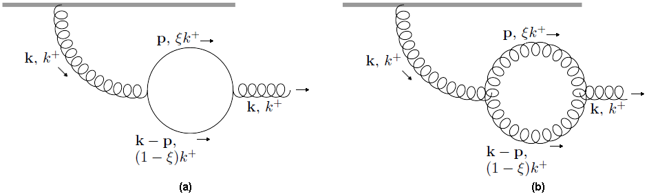
In this section, we compute the LCWF |ψ⟩|\psi\rangle perturbatively in Hi​n​tH_{int}, up to order g3g^{3}. Normalisation of the LCWF is done to order g4g^{4}. Apart of the usual technical aspects, such as divergencies, related to loop calculations, there are two unfamiliar subtleties. The first one originates from the fact that the matrix elements of Hi​n​tH_{int} (2.11) over the soft states defined in section 2.4 are non-commuting operators on the valence Hilbert space. We thus have to revise the standard perturbation theory in order to account for non-commutativity of the matrix elements, carefully tracing their ordering. This is done in Appendix E. The second subtlety is related to the Born-Oppenheimer approximation and its applicability. It leads to a non-trivial condition on the phase of the LCWF, which otherwise cannot be determined from the perturbation theory. Summary of our results is presented in section 3.5.

3.1 Third Order Perturbation Theory

General perturbative expression for the wave function before normalisation, correct up to order g3g^{3}, is computed in Appendix E. After simplifying notations (|n(i)⟩⟶|i⟩\left|n^{(i)}\right\rangle\longrightarrow\left|i\right\rangle) and also normalising the state when dividing by its norm:

|ψN​L​O⟩\displaystyle\left|\psi^{NLO}\right\rangle =𝒩N​L​O|0⟩−|i⟩⟨i​|Hi​n​t|​0⟩Ei+|i⟩⟨i​|Hi​n​t|​j⟩​⟨j​|Hi​n​t|​0⟩Ei​Ej\displaystyle=\,\mathcal{N}^{NLO}\left|0\right\rangle\,-\,\left|i\right\rangle\,\frac{\left\langle i\left|H_{int}\right|0\right\rangle}{E_{i}}\,+\,\left|i\right\rangle\,\frac{\left\langle i\left|H_{int}\right|j\right\rangle\,\left\langle j\left|H_{int}\right|0\right\rangle}{E_{i}\,E_{j}}\, (3.75)
−|i⟩⟨i​|Hi​n​t|​k⟩​⟨k​|Hi​n​t|​j⟩​⟨j​|Hi​n​t|​0⟩Ei​Ej​Ek+|i⟩|⟨j​|Hi​n​t|​0⟩|2​⟨i​|Hi​n​t|​0⟩​(Ei+ 2​Ej)2​Ei2​Ej2.\displaystyle-\,\left|i\right\rangle\,\frac{\left\langle i\left|H_{int}\right|k\right\rangle\,\left\langle k\left|H_{int}\right|j\right\rangle\,\left\langle j\left|H_{int}\right|0\right\rangle}{E_{i}\,E_{j}\,E_{k}}+\,\left|i\right\rangle\,\frac{\left|\left\langle j\left|H_{int}\right|0\right\rangle\right|^{2}\left\langle i\left|H_{int}\right|0\right\rangle\,(E_{i}\,+\,2E_{j})}{2E_{i}^{2}\,E_{j}^{2}}.

Compared to Appendix E, the extra term |i⟩|⟨j​|Hi​n​t|​0⟩|2​⟨i​|Hi​n​t|​0⟩Ei2​Ej\left|i\right\rangle\,\frac{\left|\left\langle j\left|H_{int}\right|0\right\rangle\right|^{2}\left\langle i\left|H_{int}\right|0\right\rangle}{E_{i}^{2}\,E_{j}}is a contribution to the norm from the first order perturbation theory. Up to phase, 𝒩N​L​O\mathcal{N}^{NLO} is determined from normalisation of the state:

‖𝒩N​L​O‖\displaystyle\left\|\mathcal{N}^{NLO}\right\| ≡ 1−|⟨i​|Hi​n​t|​0⟩|22​Ei2+⟨0​|Hi​n​t|​i⟩​⟨i​|Hi​n​t|​j⟩​⟨j​|Hi​n​t|​0⟩2​Ei​Ej​(1Ei+1Ej)\displaystyle\equiv\,1\,-\,\frac{\left|\left\langle i\left|H_{int}\right|0\right\rangle\right|^{2}}{2E_{i}^{2}}\,+\,\frac{\left\langle 0\left|H_{int}\right|i\right\rangle\,\left\langle i\left|H_{int}\right|j\right\rangle\,\left\langle j\left|H_{int}\right|0\right\rangle}{2E_{i}\,E_{j}}\left(\frac{1}{E_{i}}\,+\,\frac{1}{E_{j}}\right) (3.76)
−⟨0​|Hi​n​t|​i⟩​⟨i​|Hi​n​t|​j⟩​⟨j​|Hi​n​t|​k⟩​⟨k​|Hi​n​t|​0⟩2​Ei​Ej​Ek​(1Ei+1Ej+1Ek)\displaystyle-\,\frac{\left\langle 0\left|H_{int}\right|i\right\rangle\,\left\langle i\left|H_{int}\right|j\right\rangle\,\left\langle j\left|H_{int}\right|k\right\rangle\,\left\langle k\left|H_{int}\right|0\right\rangle}{2E_{i}\,E_{j}\,E_{k}}\left(\frac{1}{E_{i}}\,+\,\frac{1}{E_{j}}\,+\,\frac{1}{E_{k}}\right)\,
+3​|⟨j​|Hi​n​t|​0⟩|2​|⟨i​|Hi​n​t|​0⟩|28​Ei2​Ej2.\displaystyle+\,\frac{3\left|\left\langle j\left|H_{int}\right|0\right\rangle\right|^{2}\,\left|\left\langle i\left|H_{int}\right|0\right\rangle\right|^{2}}{8E_{i}^{2}\,E_{j}^{2}}.

Summation over repeated indices ii, jj and kk is over the eigenstates of free Hamiltonian H0H_{0}, excluding the vacuum state |0⟩\left|0\right\rangle. The ones that are relevant for the NLO calculation are defined in (2.26), (2.27), and (2.28). EiE_{i} denotes the energy of the respective eigenstate, and Hi​n​tH_{int} is defined by (2.11). (3.75) is correct even when the matrix elements are operator valued and do not commute with each other. Notice that the overall phase of the wave function is not determined by the expansion (3.76). We will discuss below how this phase can be nevertheless uniquely fixed.

Our objective is to compute |ψN​L​O⟩\left|\psi^{NLO}\right\rangle. It is convenient to split the wave function according to its soft component content:

|ψN​L​O⟩=𝒩N​L​O|0⟩+|ψg​ρL​O⟩+∑i=1i=2|ψq​q¯i⟩+∑i=1i=3|ψg​gi⟩+∑i=1i=8|ψgi⟩,\left|\psi^{NLO}\right\rangle\,=\,\mathcal{N}^{NLO}\left|0\right\rangle\,+\,\left|\psi_{g\>\rho}^{LO}\right\rangle\,+\,\sum_{i=1}^{i=2}\left|\psi_{q\bar{q}}^{i}\right\rangle\,+\,\sum_{i=1}^{i=3}\left|\psi_{gg}^{i}\right\rangle\,+\,\sum_{i=1}^{i=8}\left|\psi_{g}^{i}\right\rangle, (3.77)

where the subscripts gg, g​ggg and q​q¯q\bar{q} correspond to the soft particle content in each state. |ψg​ρL​O⟩\left|\psi_{g\>\rho}^{LO}\right\rangle is the LO contribution (see section 2.7):

|ψg​ρL​O⟩=−∫Λeδ​𝖸​Λdk+∫d2​𝐤(2​π)2g​𝐤i​ρa​(−𝐤)π​k+​𝐤2|gia(k)⟩=∫Λeδ​𝖸​Λd​k+k+∫𝐱,𝐳i​g​ρa​(𝐱)​Xi2​π3/2​X2|gia(k+,𝐳)⟩.\begin{split}\left|\psi_{g\>\rho}^{LO}\right\rangle=-\int_{\Lambda}^{e^{\delta\mathsf{Y}}\Lambda}dk^{+}\int\frac{d^{2}\mathbf{k}}{(2\pi)^{2}}\frac{g\mathbf{k}^{i}\rho^{a}(-\mathbf{k})}{\sqrt{\pi k^{+}}\mathbf{k}^{2}}\left|g_{i}^{a}(k)\right\rangle=\int_{\Lambda}^{e^{\delta\mathsf{Y}}\Lambda}\frac{dk^{+}}{\sqrt{k^{+}}}\int_{\mathbf{x},\mathbf{z}}\frac{ig\rho^{a}(\mathbf{x})X^{i}}{2\pi^{3/2}X^{2}}\left|g_{i}^{a}(k^{+},\mathbf{z})\right\rangle.\end{split} (3.78)

The following states (integration over the momenta and summation over the quantum numbers of each particle are assumed) contribute and will be computed one by one below.
Order g2g^{2} states:

|ψq​q¯1⟩≡|q¯q⟩⟨q¯q|Hg​q​q|g⟩⟨g|Hg|0⟩/Eq​q¯Eg,\hskip 5.69046pt\left|\psi_{q\bar{q}}^{1}\right\rangle\,\equiv\,\left|\overline{q}\,q\right\rangle\left\langle\overline{q}\,q\left|H_{gqq}\right|g\right\rangle\left\langle g\left|H_{g}\right|0\right\rangle/E_{q\bar{q}}\,E_{g}, (3.79)
|ψq​q¯2⟩≡−|q¯q⟩⟨q¯q|Hq​q−i​n​s​t|0⟩/Eq​q¯,\hskip-28.45274pt\left|\psi_{q\bar{q}}^{2}\right\rangle\,\equiv\,-\left|\overline{q}\,q\right\rangle\left\langle\overline{q}\,q\left|H_{qq-inst}\right|0\right\rangle/E_{q\bar{q}}, (3.80)
|ψg​g1⟩≡|gg⟩⟨gg|Hg|g⟩⟨g|Hg|0⟩/Eg​gEg,\left|\psi_{gg}^{1}\right\rangle\,\equiv\,\left|g\,g\right\rangle\left\langle g\,g\left|H_{g}\right|g\right\rangle\left\langle g\left|H_{g}\right|0\right\rangle/E_{gg}\,E_{g}, (3.81)
|ψg​g2⟩≡|gg⟩⟨gg|Hg​g​g|g⟩⟨g|Hg|0⟩/Eg​gEg,\hskip 8.5359pt\left|\psi_{gg}^{2}\right\rangle\,\equiv\,\left|g\,g\right\rangle\left\langle g\,g\left|H_{ggg}\right|g\right\rangle\left\langle g\left|H_{g}\right|0\right\rangle/E_{gg}\,E_{g}, (3.82)
|ψg​g3⟩≡−|gg⟩⟨gg|Hg​g−i​n​s​t|0⟩/Eg​g.\hskip-25.6073pt\left|\psi_{gg}^{3}\right\rangle\,\equiv\,-\left|g\,g\right\rangle\left\langle g\,g\left|H_{gg-inst}\right|0\right\rangle/E_{gg}. (3.83)

Order g3g^{3} states:

|ψg1⟩≡−|g⟩⟨g|Hg​q​q|q¯q⟩⟨q¯q|Hg​q​q|g1⟩⟨g1|Hg|0⟩/EgEq​q¯Eg1,\hskip-19.91684pt\left|\psi_{g}^{1}\right\rangle\,\equiv\,-\left|g\right\rangle\left\langle g\left|H_{gqq}\right|\overline{q}\,q\right\rangle\left\langle\overline{q}\,q\left|H_{gqq}\right|g_{1}\right\rangle\left\langle g_{1}\left|H_{g}\right|0\right\rangle/E_{g}\,E_{q\bar{q}}\,E_{g_{1}}, (3.84)
|ψg2⟩≡−|g⟩⟨g|Hg​g​g|gg⟩⟨gg|Hg​g​g|g1⟩⟨g1|Hg|0⟩/EgEg​gEg1,\hskip-17.07182pt\left|\psi_{g}^{2}\right\rangle\,\equiv\,-\left|g\right\rangle\left\langle g\left|H_{ggg}\right|g\,g\right\rangle\left\langle g\,g\left|H_{ggg}\right|g_{1}\right\rangle\left\langle g_{1}\left|H_{g}\right|0\right\rangle/E_{g}\,E_{gg}\,E_{g_{1}}, (3.85)
|ψg3⟩≡|g⟩⟨g|Hg​g−i​n​s​t|g1⟩⟨g1|Hg|0⟩/EgEg1,\hskip-96.73918pt\left|\psi_{g}^{3}\right\rangle\,\equiv\,\left|g\right\rangle\left\langle g\left|H_{gg-inst}\right|g_{1}\right\rangle\left\langle g_{1}\left|H_{g}\right|0\right\rangle/E_{g}\,E_{g_{1}}, (3.86)
|ψg4⟩≡|g⟩⟨g|Hg|gg⟩⟨gg|Hg​g−i​n​s​t|0⟩/EgEg​g,\hskip-91.04872pt\left|\psi_{g}^{4}\right\rangle\,\equiv\,\left|g\right\rangle\left\langle g\left|H_{g}\right|g\,g\right\rangle\left\langle g\,g\left|H_{gg-inst}\right|0\right\rangle/E_{g}\,E_{gg}, (3.87)
|ψg5⟩≡−|g⟩⟨g|Hg|gg⟩⟨gg|Hg|g1⟩⟨g1|Hg|0⟩/EgEg​gEg1,\hskip-34.14322pt\left|\psi_{g}^{5}\right\rangle\,\equiv\,-\left|g\right\rangle\left\langle g\left|H_{g}\right|g\,g\right\rangle\left\langle g\,g\left|H_{g}\right|g_{1}\right\rangle\left\langle g_{1}\left|H_{g}\right|0\right\rangle/E_{g}\,E_{gg}\,E_{g_{1}}, (3.88)
|ψg6⟩≡−|g⟩⟨g|Hg​g​g|gg⟩⟨gg|Hg|g1⟩⟨g1|Hg|0⟩/EgEg​gEg1,\hskip-25.6073pt\left|\psi_{g}^{6}\right\rangle\,\equiv\,-\left|g\right\rangle\left\langle g\left|H_{ggg}\right|g\,g\right\rangle\left\langle g\,g\left|H_{g}\right|g_{1}\right\rangle\left\langle g_{1}\left|H_{g}\right|0\right\rangle/E_{g}\,E_{gg}\,E_{g_{1}}, (3.89)
|ψg7⟩≡−|g⟩⟨g|Hg|gg⟩⟨gg|Hg​g​g|g1⟩⟨g1|Hg|0⟩/EgEg​gEg1,\hskip-25.6073pt\left|\psi_{g}^{7}\right\rangle\,\equiv\,-\left|g\right\rangle\left\langle g\left|H_{g}\right|g\,g\right\rangle\left\langle g\,g\left|H_{ggg}\right|g_{1}\right\rangle\left\langle g_{1}\left|H_{g}\right|0\right\rangle/E_{g}\,E_{gg}\,E_{g_{1}}, (3.90)
|ψg8⟩≡|g⟩⟨g|Hg|0⟩|⟨g1|Hg|0⟩|2(2Eg1+Eg)/2Eg2Eg12.\hskip-56.9055pt\left|\psi_{g}^{8}\right\rangle\,\equiv\,\left|g\right\rangle\left\langle g\left|H_{g}\right|0\right\rangle\left|\left\langle g_{1}\left|H_{g}\right|0\right\rangle\right|^{2}(2E_{g_{1}}+E_{g})/2E_{g}^{2}\,E_{g_{1}}^{2}. (3.91)

The following contributions vanish:

−|g⟩⟨g|Hg​g​g|gg⟩⟨gg|Hg​g−i​n​s​t|g1⟩⟨g1|Hg|0⟩/EgEg​gEg1= 0,-\left|g\right\rangle\left\langle g\left|H_{ggg}\right|g\,g\right\rangle\left\langle g\,g\left|H_{gg-inst}\right|g_{1}\right\rangle\left\langle g_{1}\left|H_{g}\right|0\right\rangle/E_{g}\,E_{gg}\,E_{g_{1}}\,=\,0, (3.92)
−|g⟩⟨g|Hg​g−i​n​s​t|gg⟩⟨gg|Hg​g​g|g1⟩⟨g1|Hg|0⟩/EgEg​gEg1= 0,-\left|g\right\rangle\left\langle g\left|H_{gg-inst}\right|g\,g\right\rangle\left\langle g\,g\left|H_{ggg}\right|g_{1}\right\rangle\left\langle g_{1}\left|H_{g}\right|0\right\rangle/E_{g}\,E_{gg}\,E_{g_{1}}\,=\,0, (3.93)
|g⟩⟨g|Hg​g​g​g|g1⟩⟨g1|Hg|0⟩/EgEg¯1= 0.\left|g\right\rangle\left\langle g\left|H_{gggg}\right|g_{1}\right\rangle\left\langle g_{1}\left|H_{g}\right|0\right\rangle/E_{g}\,E_{\bar{g}_{1}}\,=\,0. (3.94)

3.2 Matrix Elements

We write down all the matrix elements that are relevant for the NLO calculation. These expressions are computed based on (2.35) −- (2.40). At NLO there are two matrix elements for the soft-soft interactions and four matrix elements for the soft-valence interactions:
∙\bullet  Gluon splits into quark and anti-quark pair

⟨q¯λ2β​(q)​qλ1α​(p)​|Hg​q​q|​gia​(k)⟩=g​tα​βa8​π3/2​k+​χλ1†​[2​𝐤ik+−σ⋅𝐩p+​σi−σi​σ⋅𝐪q+]​χλ2​δ(3)​(k−p−q).\begin{split}\left\langle\overline{q}_{\lambda_{2}}^{\beta}(q)\,q_{\lambda_{1}}^{\alpha}(p)\left|H_{gqq}\right|g_{i}^{a}(k)\right\rangle=\frac{gt_{\alpha\beta}^{a}}{8\pi^{3/2}\sqrt{k^{+}}}\chi_{\lambda_{1}}^{\dagger}\left[\frac{2\mathbf{k}^{i}}{k^{+}}-\frac{\sigma\cdot\mathbf{p}}{p^{+}}\sigma^{i}-\sigma^{i}\frac{\sigma\cdot\mathbf{q}}{q^{+}}\right]\chi_{\lambda_{2}}\delta^{(3)}(k-p-q).\end{split} (3.95)

∙\bullet  Triple gluon interaction

⟨glc(q)gnb(p)|Hg​g​g|gma(k)⟩=i​g​fa​b​c​δ(3)​(k−p−q)8​π3/2​k+​p+​q+[(𝐩m−𝐪m+q+−p+k+𝐤m)δn​l\displaystyle\left\langle g_{l}^{c}(q)\,g_{n}^{b}(p)\left|H_{ggg}\right|g_{m}^{a}(k)\right\rangle=\frac{igf^{abc}\delta^{(3)}(k-p-q)}{8\pi^{3/2}\sqrt{k^{+}p^{+}q^{+}}}\left[\left(\mathbf{p}^{m}-\mathbf{q}^{m}+\frac{q^{+}-p^{+}}{k^{+}}\mathbf{k}^{m}\right)\delta_{nl}\right.
+(𝐤n+𝐪n−k++q+p+𝐩n)δm​l+(k++p+q+𝐪l−𝐩l−𝐤l)δm​n].\displaystyle\quad\quad\quad\left.+\left(\mathbf{k}^{n}+\mathbf{q}^{n}-\frac{k^{+}+q^{+}}{p^{+}}\mathbf{p}^{n}\right)\delta_{ml}+\left(\frac{k^{+}+p^{+}}{q^{+}}\mathbf{q}^{l}-\mathbf{p}^{l}-\mathbf{k}^{l}\right)\delta_{mn}\right]. (3.96)

∙\bullet  Valence adds an extra gluon to an existing one

⟨glc​(q)​gjb​(p)​|Hg|​gia​(k)⟩=δa​c​δi​l​δ(3)​(k−q)​g​𝐩j​ρb​(−𝐩)4​π3/2​|p+|3/2+δa​b​δi​j​δ(3)​(k−p)​g​𝐪l​ρc​(−𝐪)4​π3/2​|q+|3/2.\left\langle g_{l}^{c}(q)\,g_{j}^{b}(p)\left|H_{g}\right|g_{i}^{a}(k)\right\rangle\,=\,\delta^{ac}\delta_{il}\delta^{(3)}(k-q)\,\frac{g\mathbf{p}^{j}\rho^{b}(-\mathbf{p})}{4\pi^{3/2}|p^{+}|^{3/2}}\,+\,\delta^{ab}\delta_{ij}\delta^{(3)}(k-p)\,\frac{g\mathbf{q}^{l}\rho^{c}(-\mathbf{q})}{4\pi^{3/2}|q^{+}|^{3/2}}. (3.97)

∙\bullet  Valence instantaneously creates a quark and anti-quark pair

⟨q¯λ2β​(q)​qλ1α​(p)​|Hq​q−i​n​s​t|​0⟩=g2​tα​βa​ρa​(−𝐩−𝐪)8​π3​(p++q+)2​χλ1†​χλ2.\left\langle\overline{q}_{\lambda_{2}}^{\beta}(q)\,q_{\lambda_{1}}^{\alpha}(p)\left|H_{qq-inst}\right|0\right\rangle\,=\,\frac{g^{2}t_{\alpha\beta}^{a}\rho^{a}(-\mathbf{p}-\mathbf{q})}{8\pi^{3}(p^{+}+q^{+})^{2}}\chi_{\lambda_{1}}^{\dagger}\chi_{\lambda_{2}}. (3.98)

∙\bullet  Valence instantaneously creates two gluons

⟨gjc​(q)​gib​(p)​|Hg​g−i​n​s​t|​0⟩=i​g2​fa​b​c​(q+−p+)​δi​j​ρa​(−𝐩−𝐪)2​(2​π)3​p+​q+​(p++q+)2.\left\langle g_{j}^{c}(q)\,g_{i}^{b}(p)\left|H_{gg-inst}\right|0\right\rangle\,=\,\frac{ig^{2}f^{abc}(q^{+}-p^{+})\delta_{ij}\rho^{a}(-\mathbf{p}-\mathbf{q})}{2(2\pi)^{3}\sqrt{p^{+}q^{+}}(p^{+}+q^{+})^{2}}. (3.99)

∙\bullet  Valence instantaneously interacts with a soft gluon

⟨gjc​(q)​|Hg​g−i​n​s​t|​gib​(p)⟩=i​g2​fa​b​c​(p++q+)​δi​j​ρa​(𝐩−𝐪)2​(2​π)3​p+​q+​(p+−q+)2.\left\langle g_{j}^{c}(q)\left|H_{gg-inst}\right|g_{i}^{b}(p)\right\rangle\,=\,\frac{ig^{2}f^{abc}(p^{+}+q^{+})\delta_{ij}\rho^{a}(\mathbf{p}-\mathbf{q})}{2(2\pi)^{3}\sqrt{p^{+}q^{+}}(p^{+}-q^{+})^{2}}. (3.100)

3.3 Technical Aspects of the Calculation

Before diving into the calculation of the LCWF (3.75) in the next subsection, let us first introduce several important technical aspect, which are used throughout this calculation.

∙\bullet The Decomposition Procedure

As explained in the Introduction, the result of the calculation of the LCWF will have the form (1.2). Many of the terms we are to compute will have a product of more than one ρ\rho operator. These operators do not commute and their mutual ordering is very important. (3.75) will be later used to compute the NLO JIMWLK Hamiltonian. In order to compare with section 2.8, we would have to represent our result as in (2.62), including the symmetry properties for the kernels (the ones mentioned at the end of section 2.8). These symmetry properties do not come automatically in our calculation and we would have to manipulate our final results. It turns out that in order to achieve this, it suffices to symmetrise any product of two ρ\rho operators in the LCWF via the following identity:

ρb​(−𝐤+𝐩)​ρa​(−𝐩)=12​[ρb​(−𝐤+𝐩),ρa​(−𝐩)]+12​{ρb​(−𝐤+𝐩),ρa​(−𝐩)}=i2​fb​a​d​ρd​(−𝐤)+12​{ρb​(−𝐤+𝐩),ρa​(−𝐩)}.\begin{split}&\rho^{b}(-\mathbf{k}+\mathbf{p})\,\rho^{a}(-\mathbf{p})\,=\,\frac{1}{2}\left[\rho^{b}(-\mathbf{k}+\mathbf{p}),\,\rho^{a}(-\mathbf{p})\right]\,+\,\frac{1}{2}\left\{\rho^{b}(-\mathbf{k}+\mathbf{p}),\,\rho^{a}(-\mathbf{p})\right\}\\ &=\,\frac{i}{2}f^{bad}\rho^{d}(-\mathbf{k})\,+\,\frac{1}{2}\left\{\rho^{b}(-\mathbf{k}+\mathbf{p}),\,\rho^{a}(-\mathbf{p})\right\}.\end{split} (3.101)

The replacement (3.101) will be referred to as “decomposition procedure”. The physics behind this decomposition is that it explicitly separates between contributions from two emitters being in different transverse points in coordinate space from that when both emitters are in the same point. The latter is then equivalent to a contribution from a single emitter, in accordance to the colour algebra. After implementing the decomposition procedure where applicable, each component of the LCWF will receive an extra label in accord to the number of ρ\rho operators it contains. For example, in section 3.4.1 we show that |ψq​q¯1⟩\left|\psi_{q\bar{q}}^{1}\right\rangle contains only one ρ\rho operator, and this component will be denoted thereafter by |ψq​q¯​ρ1⟩\left|\psi_{q\bar{q}\>\rho}^{1}\right\rangle.

∙\bullet Regularisation of Divergent Integrals

There are two types of divergencies that appear throughout the calculation. These are the usual divergencies in loop calculations. First, we will face divergencies that come from the longitudinal phase space integrals of the type ∫d​k+/k+\int dk^{+}/k^{+}, which correspond to emission of soft partons, just as in the case of LO calculation. These divergencies are regularised by confining the soft modes to live within the window Λ<k+<Λ​eδ​Y\Lambda<k^{+}<\Lambda e^{\delta Y}. When computing the Hamiltonian in the next section, we will also encounter this longitudinal divergence "squared". Physically, such double divergence corresponds to independent (uncorrelated) emission of two soft gluons, which is accounted for by iteration of the LO Hamiltonian.

Λ\Lambda acts as an IR cutoff which will be set to zero (and δ​Y\delta Y to infinity) whenever it is safe to do so, without stating it explicitly.

UV divergences in transverse space integrals will be treated via dimensional regularisation, switching to d≡ 2−ϵd\,\equiv\,2\,-\,\epsilon dimensions,

∫d2​𝐩(2​π)2⟶μϵ​∫dd​𝐩(2​π)d.\int\frac{d^{2}\mathbf{p}}{(2\pi)^{2}}\,\longrightarrow\,\mu^{\epsilon}\int\frac{d^{d}\mathbf{p}}{(2\pi)^{d}}. (3.102)

In addition, we will be frequently using the identity:

∫dd​𝐩​F​(𝐩2)​𝐩i​𝐩j=δi​jd​∫dd​𝐩​F​(𝐩2)​𝐩2.\begin{split}\int d^{d}\mathbf{p}\,F(\mathbf{p}^{2})\,\mathbf{p}^{i}\,\mathbf{p}^{j}\,=\,\frac{\delta^{ij}}{d}\int d^{d}\mathbf{p}\,F(\mathbf{p}^{2})\,\mathbf{p}^{2}.\end{split} (3.103)

A couple of relevant integrals in dimensional regularisation are quoted in Appendix C. As usual, (C.321) will be used for ϵ\epsilon expansion. We will retain the divergent 1ϵ\frac{1}{\epsilon} terms at the level of the wave function, as by itself the wave function is not a physical observable. Coupling constant renormalisation is done for physical observables, such as Σ\Sigma (or the JIMWLK Hamiltonian). This will be implemented in the M​S¯\overline{MS} scheme as a default action without any further explanations. The calculation also involves overlapping singularities when both the longitudinal and transverse integrals diverge. Those are treated similarly as above.

In addition to the above discussed UV divergencies, there are also potential IR divergencies at small transverse momenta. Those, however, do not emerge in our calculation explicitly because they always get regularised by the charge density operators ρ\rho. Yet, this depends on a non-specified IR behaviour of the valence degrees of freedom and a priori is not guaranteed to lead to a safe IR. Particularly the IR divergencies resurface when the resulting JIMWLK Hamiltonian is taken to act on a gauge non-invariant operator, such as in the problem of gluon reggeization. The gluon trajectory is then found to be IR divergent even at LO.

∙\bullet Phase of the LCWF

The perturbation theory cannot fix the phase of the LCWF, that is the phase of 𝒩N​L​O{\cal N}^{NLO}. Normally, the phase is unobservable as it cancels in physical observables. However, this is not the case at hand, as we are not computing the full wave function but only its soft component. The normalisation coefficient 𝒩N​L​O{\cal N}^{NLO} is operator valued on the valence Hilbert space and thus its phase can make a non-trivial contribution to the observables.

How can we find this phase which is clearly beyond the perturbation theory? We recall that our formalism is based on the Born-Oppenheimer adiabatic approximation33 3 We would like to specially thank Alex Kovner who significantly helped us to establish the argument.. Obviously, there is some freedom in the phase, as, in principle, it can be always absorbed into the valence part of the LCWF. Yet, the factorisation (2.24) assumes that

⟨v|⊗⟨ψ|HV|ψ⟩⊗|v⟩≃⟨v|HV|v⟩or⟨ψ|HV|ψ⟩s​o​f​t≃ 0.\langle v|\otimes\langle\psi|\,H_{V}\,|\psi\rangle\otimes|v\rangle\,\simeq\,\langle v|\,H_{V}\,|v\rangle\,~~~~or~~~~~\left\langle\psi\right|\,H_{V}\,\left|\psi\right\rangle_{soft}\,\simeq\,0\,. (3.104)

where HVH_{V} is a Hamiltonian for the valence degrees of freedom. The second expectation value is taken over the soft modes only. The condition (3.104) means that the dynamics of the soft modes does not significantly affect that of the valence. This assumption is implicit in the way the high energy factorisation is set, eliminating the freedom in the phase.

While the explicit form of HVH_{V} is not known, the condition (3.104) presumably should be valid for any operator on the valence Hilbert space. Particularly, HVH_{V} can be thought as been constructed from some powers of ρ\rho, with (3.104) implying that they commute with |ψ⟩|\psi\rangle on the valence Hilbert space. Commuting one ρ\rho with |ψ⟩|\psi\rangle is equivalent to taking derivative δ/δ​ρ\delta/\delta\rho. We thus require the following condition to hold

⟨ψ|δδ​ρd​(𝐰)|ψ⟩= 0.\left\langle\psi\right|\,\frac{\delta}{\delta\rho^{d}(\mathbf{w})}\,\left|\psi\right\rangle\,=\,0\,. (3.105)

Notice that (3.105) is the Berry connection, which we require to vanish. It is easy to check that at LO the condition is fulfilled by |ψL​O⟩|\psi^{LO}\rangle automatically. At NLO, this condition becomes a non-trivial constraint on the phase, which is worked out in Appendix F.

3.4 Computation of the NLO Wave Function

In this section we compute the wave function (3.75). For each of the contributions (3.79) - (3.91), a separate subsection is devoted. Lengthy computations are available in Appendix G. The reader who is not interested in these details can proceed directly to the final results in section 3.5.

3.4.1 Quark anti−-Quark State

Computation of |ψq​q¯1⟩\left|\psi_{q\bar{q}}^{1}\right\rangle

|ψq​q¯​ρ1⟩\left|\psi_{q\bar{q}\>\rho}^{1}\right\rangle is defined in (3.79) (Fig. 4a).

      Refer to caption

Figure 4: Quark and anti-quark emission diagrams. The bold black line over the gluon in (b)(b) marks the instantaneous interaction. (a)(a) - |ψq​q¯1⟩\left|\psi_{q\bar{q}}^{1}\right\rangle, (b)(b) - |ψq​q¯2⟩\left|\psi_{q\bar{q}}^{2}\right\rangle.
|ψq​q¯1⟩≡∑λ1,λ2,f∫Λeδ​𝖸​Λd​k+​d​p+​d​q+​∫d2​𝐤​d2​𝐩​d2​𝐪×|q¯λ2β,f(q)qλ1α,f(p)⟩⟨q¯λ2β,f​(q)​qλ1α,f​(p)​|Hg​q​q|​gia​(k)⟩​⟨gia​(k)​|Hg|​0⟩Eq​q¯​(p,q)​Eg​(k).\begin{split}\left|\psi_{q\bar{q}}^{1}\right\rangle&\equiv\,\sum_{\lambda_{1},\lambda_{2},f}\int_{\Lambda}^{e^{\delta\mathsf{Y}}\Lambda}dk^{+}\,dp^{+}\,dq^{+}\,\int d^{2}\mathbf{k}\,d^{2}\mathbf{p}\,d^{2}\mathbf{q}\\ &\times\left|\bar{q}_{\lambda_{2}}^{\beta,\,f}(q)\,q_{\lambda_{1}}^{\alpha,\,f}(p)\right\rangle\frac{\left\langle\bar{q}_{\lambda_{2}}^{\beta,\,f}(q)\,q_{\lambda_{1}}^{\alpha,\,f}(p)\left|H_{gqq}\right|g_{i}^{a}(k)\right\rangle\left\langle g_{i}^{a}(k)\left|H_{g}\right|0\right\rangle}{E_{q\bar{q}}(p,\,q)\,E_{g}(k)}.\end{split} (3.106)

The physics content of (3.106) becomes clear by reading the matrix elements from the right to left: the first one corresponds to initial emission of a soft gluon from the valence current; then this soft gluon subsequently splits to a quark and anti-quark pair. The momentum conservation δ(3)​(q−k+p)\delta^{(3)}(q-k+p), which is explicit in the second matrix element (3.95), removes qq integral and effectively turns it into k−pk-p. The process is illustrated in Fig. 4a.

After inserting the relevant matrix elements, (2.55) and (3.95), and integrating over qq:

|ψq​q¯​ρ1⟩≡|ψq​q¯1⟩=∑λ1,λ2,f∫Λeδ​𝖸​Λdk+∫01dξ∫d2𝐤d2𝐩4​ξ​(1−ξ)((1−ξ)​𝐩2+ξ​(𝐤−𝐩)2)​𝐤2×(g​tα​βa8​π3/2​χλ1†​[2​𝐤i−σ⋅𝐩ξ​σi−σi​σ⋅(𝐤−𝐩)1−ξ]​χλ2)​(g​ρa​(−𝐤)​𝐤i4​π3/2)×|q¯λ2β,f((1−ξ)k+,𝐤−𝐩)qλ1α,f(ξk+,𝐩)⟩.\begin{split}&\left|\psi_{q\bar{q}\>\rho}^{1}\right\rangle\,\equiv\,\left|\psi_{q\bar{q}}^{1}\right\rangle\,=\,\sum_{\lambda_{1},\lambda_{2},f}\int_{\Lambda}^{e^{\delta\mathsf{Y}}\Lambda}dk^{+}\,\int_{0}^{1}d\xi\,\int d^{2}\mathbf{k}\,d^{2}\mathbf{p}\>\frac{4\xi(1-\xi)}{\left((1-\xi)\mathbf{p}^{2}+\xi(\mathbf{k}-\mathbf{p})^{2}\right)\mathbf{k}^{2}}\\ &\times\left(\frac{gt_{\alpha\beta}^{a}}{8\pi^{3/2}}\chi_{\lambda_{1}}^{\dagger}\left[2\mathbf{k}^{i}-\frac{\sigma\cdot\mathbf{p}}{\xi}\sigma^{i}-\sigma^{i}\frac{\sigma\cdot(\mathbf{k}-\mathbf{p})}{1-\xi}\right]\chi_{\lambda_{2}}\right)\left(\frac{g\rho^{a}(-\mathbf{k})\mathbf{k}^{i}}{4\pi^{3/2}}\right)\\ &\times\left|\bar{q}_{\lambda_{2}}^{\beta,\,f}((1-\xi)k^{+},\,\mathbf{k}-\mathbf{p})\,q_{\lambda_{1}}^{\alpha,\,f}(\xi k^{+},\,\mathbf{p})\right\rangle.\end{split} (3.107)

The variable ξ\xi is defined as:

ξ≡p+k+.\xi\,\equiv\,\frac{p^{+}}{k^{+}}. (3.108)

This definition will be used repeatedly throughout this paper.

Computation of |ψq​q¯2⟩\left|\psi_{q\bar{q}}^{2}\right\rangle

|ψq​q¯​ρ2⟩\left|\psi_{q\bar{q}\>\rho}^{2}\right\rangle is defined in (3.80) (Fig. 4b).

|ψq​q¯2⟩≡−∑λ1,λ2,f∫Λeδ​𝖸​Λdk+∫0k+dp+∫d2𝐤d2𝐩×|q¯λ2β,f(k−p)qλ1α,f(p)⟩⟨q¯λ2β,f​(k−p)​qλ1α,f​(p)​|Hq​q−i​n​s​t|​0⟩Eq​q¯​(p,k−p).\begin{split}\left|\psi_{q\bar{q}}^{2}\right\rangle&\equiv\,-\sum_{\lambda_{1},\lambda_{2},f}\int_{\Lambda}^{e^{\delta\mathsf{Y}}\Lambda}dk^{+}\,\int_{0}^{k^{+}}dp^{+}\,\int d^{2}\mathbf{k}\,d^{2}\mathbf{p}\>\\ &\times\left|\bar{q}_{\lambda_{2}}^{\beta,\,f}(k-p)\,q_{\lambda_{1}}^{\alpha,\,f}(p)\right\rangle\frac{\left\langle\bar{q}_{\lambda_{2}}^{\beta,\,f}(k-p)\,q_{\lambda_{1}}^{\alpha,\,f}(p)\left|H_{qq-inst}\right|0\right\rangle}{E_{q\bar{q}}(p,\,k-p)}.\end{split} (3.109)

Inserting the matrix element (3.98) and changing variables according to (3.108):

|ψq​q¯​ρ2⟩≡|ψq​q¯2⟩=−∑λ1,λ2,f∫Λeδ​𝖸​Λdk+∫01dξ∫d2𝐤d2𝐩×g2​tα​βa​ξ​(1−ξ)​ρa​(−𝐤)​χλ1†​χλ24​π3​((1−ξ)​𝐩2+ξ​(𝐤−𝐩)2)|q¯λ2β,f((1−ξ)k+,𝐤−𝐩)qλ1α,f(ξk+,𝐩)⟩.\begin{split}\left|\psi_{q\bar{q}\>\rho}^{2}\right\rangle&\equiv\,\left|\psi_{q\bar{q}}^{2}\right\rangle=\,-\sum_{\lambda_{1},\lambda_{2},f}\int_{\Lambda}^{e^{\delta\mathsf{Y}}\Lambda}dk^{+}\,\int_{0}^{1}d\xi\,\int d^{2}\mathbf{k}\,d^{2}\mathbf{p}\>\\ &\times\frac{g^{2}t_{\alpha\beta}^{a}\xi(1-\xi)\rho^{a}(-\mathbf{k})\chi_{\lambda_{1}}^{\dagger}\chi_{\lambda_{2}}}{4\pi^{3}\left((1-\xi)\mathbf{p}^{2}+\xi(\mathbf{k}-\mathbf{p})^{2}\right)}\left|\bar{q}_{\lambda_{2}}^{\beta,\,f}((1-\xi)k^{+},\,\mathbf{k}-\mathbf{p})\,q_{\lambda_{1}}^{\alpha,\,f}(\xi k^{+},\,\mathbf{p})\right\rangle.\\ \end{split} (3.110)

3.4.2 Two Gluon State

Computation of |ψg​g1⟩\left|\psi_{gg}^{1}\right\rangle

|ψg​g1⟩\left|\psi_{gg}^{1}\right\rangle is defined in (3.81) (Fig. 5a).

  Refer to caption

Figure 5: Two gluon producation diagrams. (a) - |ψg​g1⟩\left|\psi_{gg}^{1}\right\rangle, (b) - |ψg​g2⟩\left|\psi_{gg}^{2}\right\rangle, (c) - |ψg​g3⟩\left|\psi_{gg}^{3}\right\rangle.
|ψg​g1⟩≡12​∫Λeδ​𝖸​Λd​q+​d​k+​∫Λk+−Λd​p+​∫d2​𝐪​d2​𝐤​d2​𝐩×|gjb(k−p)glc(p)⟩⟨gjb​(k−p)​glc​(p)​|Hg|​gia​(q)⟩​⟨gia​(q)​|Hg|​0⟩Eg​g​(p,k−p)​Eg​(q).\begin{split}\left|\psi_{gg}^{1}\right\rangle&\equiv\,\frac{1}{2}\int_{\Lambda}^{e^{\delta\mathsf{Y}}\Lambda}dq^{+}\,dk^{+}\,\int_{\Lambda}^{k^{+}-\Lambda}dp^{+}\,\int\,d^{2}\mathbf{q}\,d^{2}\mathbf{k}\,d^{2}\mathbf{p}\\ &\times\left|g_{j}^{b}(k-p)\,g_{l}^{c}(p)\right\rangle\frac{\left\langle g_{j}^{b}(k-p)\,g_{l}^{c}(p)\left|H_{g}\right|g_{i}^{a}(q)\right\rangle\left\langle g_{i}^{a}(q)\left|H_{g}\right|0\right\rangle}{E_{gg}(p,\,k-p)\,E_{g}(q)}.\end{split} (3.111)

Here 12\frac{1}{2} is to avoid double-counting in two-gluon states. Inserting the matrix elements, (2.55) and (3.97):

|ψg​g1⟩\displaystyle\left|\psi_{gg}^{1}\right\rangle =\displaystyle= 12​∫Λeδ​𝖸​Λd​k+​d​q+​∫Λk+−Λd​p+​∫d2​𝐤​d2​𝐩​d2​𝐪​1𝐪22​q+​(𝐩22​p++(𝐤−𝐩)22​(k+−p+))\displaystyle\frac{1}{2}\int_{\Lambda}^{e^{\delta\mathsf{Y}}\Lambda}dk^{+}\,dq^{+}\,\int_{\Lambda}^{k^{+}-\Lambda}dp^{+}\,\int d^{2}\mathbf{k}\,d^{2}\mathbf{p}\,d^{2}\mathbf{q}\,\frac{1}{\frac{\mathbf{q}^{2}}{2q^{+}}\left(\frac{\mathbf{p}^{2}}{2p^{+}}+\frac{(\mathbf{k}-\mathbf{p})^{2}}{2(k^{+}-p^{+})}\right)} (3.112)
×\displaystyle\times (δa​c​δi​l​δ(3)​(p−q)​g⁡(𝐤j−𝐩j)​ρb​(−𝐤+𝐩)4​π3/2​|k+−p+|3/2+δa​b​δj​i​δ(3)​(k−p−q)​g​𝐩l​ρc​(−𝐩)4​π3/2​|p+|3/2)\displaystyle\left(\delta^{ac}\delta_{il}\delta^{(3)}(p-q)\,\frac{g\left(\mathbf{k}^{j}-\mathbf{p}^{j}\right)\rho^{b}(-\mathbf{k}+\mathbf{p})}{4\pi^{3/2}|k^{+}-p^{+}|^{3/2}}+\delta^{ab}\delta_{ji}\delta^{(3)}(k-p-q)\,\frac{g\mathbf{p}^{l}\rho^{c}(-\mathbf{p})}{4\pi^{3/2}|p^{+}|^{3/2}}\right)
×\displaystyle\times (g​𝐪i​ρa​(−𝐪)4​π3/2​|q+|3/2)|gjb(k−p)glc(p)⟩.\displaystyle\left(\frac{g\mathbf{q}^{i}\rho^{a}(-\mathbf{q})}{4\pi^{3/2}|q^{+}|^{3/2}}\right)\left|g_{j}^{b}(k-p)\,g_{l}^{c}(p)\right\rangle.

The physics content of (3.111) is quite obvious and corresponds to subsequent emissions of two soft gluons. The momentum conservation imposed via the delta functions turns the momentum qq into either kk or k−pk-p, which is illustrated in Fig. 5a. After integration over qq, (3.112) becomes:

|ψg​g1⟩=∫Λeδ​𝖸​Λd​k+​∫d2​𝐤​d2​𝐩​∫Λk+1−Λk+d​ξ​g2​𝐩j​(𝐤i−𝐩i)8​π3​(ξ​(𝐤−𝐩)2+(1−ξ)​𝐩2)×(ρa​(−𝐤+𝐩)​ρb​(−𝐩)​ξ𝐩2​1−ξ+ρb​(−𝐩)​ρa​(−𝐤+𝐩)​1−ξ(𝐤−𝐩)2​ξ)×|gia((1−ξ)k+,𝐤−𝐩)gjb(ξk+,𝐩)⟩.\begin{split}\left|\psi_{gg}^{1}\right\rangle&=\int_{\Lambda}^{e^{\delta\mathsf{Y}}\Lambda}dk^{+}\,\int d^{2}\mathbf{k}\,d^{2}\mathbf{p}\,\int_{\frac{\Lambda}{k^{+}}}^{1-\frac{\Lambda}{k^{+}}}d\xi\,\frac{g^{2}\mathbf{p}^{j}\left(\mathbf{k}^{i}-\mathbf{p}^{i}\right)}{8\pi^{3}\left(\xi(\mathbf{k}-\mathbf{p})^{2}+(1-\xi)\mathbf{p}^{2}\right)}\\ &\times\left(\frac{\rho^{a}(-\mathbf{k}+\mathbf{p})\rho^{b}(-\mathbf{p})\sqrt{\xi}}{\mathbf{p}^{2}\sqrt{1-\xi}}\,+\,\frac{\rho^{b}(-\mathbf{p})\rho^{a}(-\mathbf{k}+\mathbf{p})\sqrt{1-\xi}}{(\mathbf{k}-\mathbf{p})^{2}\sqrt{\xi}}\right)\,\\ &\times\left|g_{i}^{a}((1-\xi)k^{+},\,\mathbf{k}-\mathbf{p})\,g_{j}^{b}(\xi k^{+},\,\mathbf{p})\right\rangle.\\ \end{split} (3.113)

Here ξ≡p+k+\xi\,\equiv\,\frac{p^{+}}{k^{+}} as already defined in (3.108).

The result (3.113) can be decomposed according to (3.101), and represented as contributions with one and two ρ\rho operators:

|ψg​g1⟩≡|ψg​g​ρ1⟩+|ψg​g​ρ​ρ⟩,\left|\psi_{gg}^{1}\right\rangle\,\equiv\,\left|\psi_{gg\>\rho}^{1}\right\rangle\,+\,\left|\psi_{gg\>\rho\rho}\right\rangle, (3.114)

with

|ψg​g​ρ1⟩\displaystyle\left|\psi_{gg\>\rho}^{1}\right\rangle ≡\displaystyle\equiv ∫Λeδ​𝖸​Λd​k+​∫d2​𝐤​d2​𝐩​∫Λk+1−Λk+d​ξ​−i​g2​fa​b​c​𝐩i​(𝐤j−𝐩j)​ρc​(−𝐤)​ξ⁡(1−ξ)16​π3​(ξ​(𝐤−𝐩)2+(1−ξ)​𝐩2)\displaystyle\int_{\Lambda}^{e^{\delta\mathsf{Y}}\Lambda}dk^{+}\,\int d^{2}\mathbf{k}\,d^{2}\mathbf{p}\,\int_{\frac{\Lambda}{k^{+}}}^{1-\frac{\Lambda}{k^{+}}}d\xi\,\frac{-ig^{2}f^{abc}\mathbf{p}^{i}\left(\mathbf{k}^{j}-\mathbf{p}^{j}\right)\rho^{c}(-\mathbf{k})\sqrt{\xi(1-\xi)}}{16\pi^{3}\left(\xi(\mathbf{k}-\mathbf{p})^{2}+(1-\xi)\mathbf{p}^{2}\right)} (3.115)
×\displaystyle\times (1(1−ξ)​𝐩2−1ξ​(𝐤−𝐩)2)|gjb((1−ξ)k+,𝐤−𝐩)gia(ξk+,𝐩)⟩,\displaystyle\left(\frac{1}{(1-\xi)\mathbf{p}^{2}}-\frac{1}{\xi(\mathbf{k}-\mathbf{p})^{2}}\right)\left|g_{j}^{b}((1-\xi)k^{+},\,\mathbf{k}-\mathbf{p})\,g_{i}^{a}(\xi k^{+},\,\mathbf{p})\right\rangle,

and

|ψg​g​ρ​ρ⟩\displaystyle\left|\psi_{gg\>\rho\rho}\right\rangle ≡\displaystyle\equiv ∫Λeδ​𝖸​Λd​k+​∫d2​𝐤​d2​𝐩​∫Λk+1−Λk+𝑑ξ\displaystyle\int_{\Lambda}^{e^{\delta\mathsf{Y}}\Lambda}dk^{+}\,\int d^{2}\mathbf{k}\,d^{2}\mathbf{p}\,\int_{\frac{\Lambda}{k^{+}}}^{1-\frac{\Lambda}{k^{+}}}d\xi\, (3.116)
×\displaystyle\times g2​𝐩i​(𝐤j−𝐩j)​{ρa​(−𝐩),ρb​(−𝐤+𝐩)}16​π3​𝐩2​(𝐤−𝐩)2​ξ⁡(1−ξ)|gjb((1−ξ)k+,𝐤−𝐩)gia(ξk+,𝐩)⟩.\displaystyle\frac{g^{2}\mathbf{p}^{i}\left(\mathbf{k}^{j}-\mathbf{p}^{j}\right)\left\{\rho^{a}(-\mathbf{p}),\,\rho^{b}(-\mathbf{k}+\mathbf{p})\right\}}{16\pi^{3}\mathbf{p}^{2}(\mathbf{k}-\mathbf{p})^{2}\sqrt{\xi(1-\xi)}}\left|g_{j}^{b}((1-\xi)k^{+},\,\mathbf{k}-\mathbf{p})\,g_{i}^{a}(\xi k^{+},\,\mathbf{p})\right\rangle.

Computation of |ψg​g2⟩\left|\psi_{gg}^{2}\right\rangle

|ψg​g2⟩\left|\psi_{gg}^{2}\right\rangle is defined in (3.82) (Fig. 5b).

|ψg​g2⟩≡12​∫Λeδ​𝖸​Λd​k+​d​p+​d​q+​∫d2​𝐤​d2​𝐩​d2​𝐪×|gjb(q)glc(p)⟩⟨gjb​(q)​glc​(p)​|Hg​g​g|​gia​(k)⟩​⟨gia​(k)​|Hg|​0⟩Eg​g​(p,q)​Eg​(k).\begin{split}\left|\psi_{gg}^{2}\right\rangle&\equiv\,\frac{1}{2}\int_{\Lambda}^{e^{\delta\mathsf{Y}}\Lambda}dk^{+}\,dp^{+}\,dq^{+}\,\int d^{2}\mathbf{k}\,d^{2}\mathbf{p}\,d^{2}\mathbf{q}\\ &\times\left|g_{j}^{b}(q)\,g_{l}^{c}(p)\right\rangle\frac{\left\langle g_{j}^{b}(q)\,g_{l}^{c}(p)\left|H_{ggg}\right|g_{i}^{a}(k)\right\rangle\left\langle g_{i}^{a}(k)\left|H_{g}\right|0\right\rangle}{E_{gg}(p,\,q)\,E_{g}(k)}.\\ \end{split} (3.117)

The condition q=k−pq=k-p is enforced via momentum conservation, which is reflected on Fig. 5b. By inserting the relevant matrix elements, (2.55) and (3.96), and integrating over qq:

|ψg​g2⟩\displaystyle\left|\psi_{gg}^{2}\right\rangle =\displaystyle= ∫Λeδ​𝖸​Λd​k+​∫Λk+d​p+​∫d2​𝐤​d2​𝐩​i​g​fa​c​b16​π3/2​(𝐩22​p++(𝐤−𝐩)22​(k+−p+))​(𝐤22​k+)​k+​p+​(k+−p+)\displaystyle\int_{\Lambda}^{e^{\delta\mathsf{Y}}\Lambda}dk^{+}\int_{\Lambda}^{k^{+}}dp^{+}\int d^{2}\mathbf{k}\,d^{2}\mathbf{p}\>\frac{igf^{acb}}{16\pi^{3/2}\left(\frac{\mathbf{p}^{2}}{2p^{+}}+\frac{(\mathbf{k}-\mathbf{p})^{2}}{2(k^{+}-p^{+})}\right)\left(\frac{\mathbf{k}^{2}}{2k^{+}}\right)\sqrt{k^{+}p^{+}(k^{+}-p^{+})}} (3.118)
×\displaystyle\times ([2​𝐩i−2​p+k+​𝐤i]​δj​l+[k++p+k+−p+​(𝐤j−𝐩j)−𝐤j−𝐩j]​δi​l+[2​𝐤l−2​k+p+​𝐩l]​δi​j)\displaystyle\left(\left[2\mathbf{p}^{i}-\frac{2p^{+}}{k^{+}}\mathbf{k}^{i}\right]\delta_{jl}+\left[\frac{k^{+}+p^{+}}{k^{+}-p^{+}}(\mathbf{k}^{j}-\mathbf{p}^{j})-\mathbf{k}^{j}-\mathbf{p}^{j}\right]\delta_{il}+\left[2\mathbf{k}^{l}-\frac{2k^{+}}{p^{+}}\mathbf{p}^{l}\right]\delta_{ij}\right)
×\displaystyle\times (g​ρa​(−𝐤)​𝐤i4​π3/2​|k+|3/2)|gjb(k−p)glc(p)⟩.\displaystyle\left(\frac{g\rho^{a}(-\mathbf{k})\mathbf{k}^{i}}{4\pi^{3/2}|k^{+}|^{3/2}}\right)\left|g_{j}^{b}(k-p)\,g_{l}^{c}(p)\right\rangle.

By introducing new variables according to (3.108) and

𝐩=ξ​𝐤+𝐩~,\mathbf{p}\,=\,\xi\mathbf{k}\,+\,\widetilde{\mathbf{p}}, (3.119)

(3.118) becomes:

|ψg​g​ρ2⟩≡|ψg​g2⟩=−∫Λeδ​𝖸​Λdk+∫d2𝐤d2𝐩~∫Λk+1−Λk+dξi​g2​fa​b​c​ρa​(−𝐤)​ξ⁡(1−ξ)​𝐤i8​π3​(𝐤2​ξ​(1−ξ)+𝐩~2)​𝐤2×(𝐩~iδj​l−11−ξ𝐩~jδi​l−1ξ𝐩~lδi​j)|gjb((1−ξ)k+,(1−ξ)𝐤−𝐩~)glc(ξk+,ξ𝐤+𝐩~)⟩.\begin{split}\left|\psi_{gg\>\rho}^{2}\right\rangle&\equiv\,\left|\psi_{gg}^{2}\right\rangle\,=\,-\int_{\Lambda}^{e^{\delta\mathsf{Y}}\Lambda}dk^{+}\,\int d^{2}\mathbf{k}\,d^{2}\widetilde{\mathbf{p}}\,\int_{\frac{\Lambda}{k^{+}}}^{1-\frac{\Lambda}{k^{+}}}d\xi\,\frac{ig^{2}f^{abc}\rho^{a}(-\mathbf{k})\sqrt{\xi(1-\xi)}\mathbf{k}^{i}}{8\pi^{3}\left(\mathbf{k}^{2}\xi(1-\xi)+\widetilde{\mathbf{p}}^{2}\right)\mathbf{k}^{2}}\\ &\times\left(\widetilde{\mathbf{p}}^{i}\delta_{jl}-\frac{1}{1-\xi}\widetilde{\mathbf{p}}^{j}\delta_{il}-\frac{1}{\xi}\widetilde{\mathbf{p}}^{l}\delta_{ij}\right)\left|g_{j}^{b}((1-\xi)k^{+},\,(1-\xi)\mathbf{k}-\widetilde{\mathbf{p}})\,g_{l}^{c}(\xi k^{+},\,\xi\mathbf{k}+\widetilde{\mathbf{p}})\right\rangle.\\ \end{split} (3.120)

Computation of |ψg​g3⟩\left|\psi_{gg}^{3}\right\rangle

|ψg​g3⟩\left|\psi_{gg}^{3}\right\rangle is defined in (3.83) (Fig. 5c.).

|ψg​g3⟩≡−12∫Λeδ​𝖸​Λdk+∫Λk+−Λdp+∫d2𝐤d2𝐩×|gib(k−p)gjc(p)⟩⟨gib​(k−p)​gjc​(p)​|Hg​g−i​n​s​t|​0⟩Eg​g​(k−p,p).\begin{split}\left|\psi_{gg}^{3}\right\rangle&\equiv\,-\frac{1}{2}\int_{\Lambda}^{e^{\delta\mathsf{Y}}\Lambda}dk^{+}\,\int_{\Lambda}^{k^{+}-\Lambda}dp^{+}\,\int d^{2}\mathbf{k}\,d^{2}\mathbf{p}\,\\ &\times\left|g_{i}^{b}(k-p)\,g_{j}^{c}(p)\right\rangle\frac{\left\langle g_{i}^{b}(k-p)\,g_{j}^{c}(p)\left|H_{gg-inst}\right|0\right\rangle}{E_{gg}(k-p,\,p)}.\\ \end{split} (3.121)

After inserting the relevant matrix element (3.98) and changing variables according to (3.108) and (3.119), we can write the last result as:

|ψg​g​ρ3⟩≡|ψg​g3⟩=∫Λeδ​𝖸​Λdk+∫d2𝐤d2𝐩~∫Λk+1−Λk+dξi​g2​fa​b​c​ρa​(−𝐤)​(1−2​ξ)​ξ⁡(1−ξ)16​π3​(𝐤2​ξ​(1−ξ)+𝐩~2)δi​j\displaystyle\left|\psi_{gg\>\rho}^{3}\right\rangle\,\equiv\,\left|\psi_{gg}^{3}\right\rangle\,=\,\int_{\Lambda}^{e^{\delta\mathsf{Y}}\Lambda}dk^{+}\,\int d^{2}\mathbf{k}\,d^{2}\widetilde{\mathbf{p}}\,\int_{\frac{\Lambda}{k^{+}}}^{1-\frac{\Lambda}{k^{+}}}d\xi\,\frac{ig^{2}f^{abc}\rho^{a}(-\mathbf{k})(1-2\xi)\sqrt{\xi(1-\xi)}}{16\pi^{3}\left(\mathbf{k}^{2}\xi(1-\xi)+\widetilde{\mathbf{p}}^{2}\right)}\delta_{ij}
×|gib((1−ξ)k+,(1−ξ)𝐤−𝐩~)gjc(ξk+,ξ𝐤+𝐩~)⟩.\displaystyle\times\left|g_{i}^{b}((1-\xi)k^{+},\,(1-\xi)\mathbf{k}-\widetilde{\mathbf{p}})\,g_{j}^{c}(\xi k^{+},\,\xi\mathbf{k}+\widetilde{\mathbf{p}})\right\rangle. (3.122)

While focusing on two-parton production, we have not encountered any divergencies. This is obviously because we have not yet ran into any loop integrations. At this stage we can only anticipate their appearance in the next section, where the overlaps of two wavefunctions are computed. Particularly, it is pretty obvious that ψq​q1\psi_{qq}^{1} will lead to the logarithmic singularity in longitudinal momenta integration squared, which corresponds to second iteration of the LO JIMWLK Hamiltonian. Somewhat less obvious, but ψq​q3\psi_{qq}^{3} also contributes to square of the LO. This is due to the kinematical region where one of the two gluons is much softer than another. In the next subsection, we will encounter both longitudinal and UV divergencies in the LCWF itself. The divergencies will be present in most of the loop corrections to the single gluon state.

3.4.3 One Gluon State

Computation of |ψg1⟩\left|\psi_{g}^{1}\right\rangle

|ψg1⟩\left|\psi_{g}^{1}\right\rangle is defined in (3.84) (Fig. 6a.).

|ψg1⟩\displaystyle\left|\psi_{g}^{1}\right\rangle ≡\displaystyle\equiv −∫Λeδ​𝖸​Λdk+dp+dq+dr+∫d2𝐤d2𝐩d2𝐪d2𝐫\displaystyle-\int_{\Lambda}^{e^{\delta\mathsf{Y}}\Lambda}dk^{+}\,dp^{+}\,dq^{+}\,dr^{+}\,\int d^{2}\mathbf{k}\,d^{2}\mathbf{p}\,d^{2}\mathbf{q}\,d^{2}\mathbf{r} (3.123)
×\displaystyle\times |gjd(r)⟩⟨gjd​(r)​|Hg​q​q|​qλ1α,f​(p)​q¯λ2β,f​(q)⟩​⟨qλ1α,f​(p)​q¯λ2β,f​(q)​|Hg​q​q|​gia​(k)⟩​⟨gia​(k)​|Hg|​0⟩Eg​(r)​Eq​q¯​(p,q)​Eg​(k).\displaystyle\left|g_{j}^{d}(r)\right\rangle\frac{\left\langle g_{j}^{d}(r)\left|H_{gqq}\right|q_{\lambda_{1}}^{\alpha,f}(p)\,\bar{q}_{\lambda_{2}}^{\beta,f}(q)\right\rangle\left\langle q_{\lambda_{1}}^{\alpha,f}(p)\,\bar{q}_{\lambda_{2}}^{\beta,f}(q)\left|H_{gqq}\right|g_{i}^{a}(k)\right\rangle\left\langle g_{i}^{a}(k)\left|H_{g}\right|0\right\rangle}{E_{g}(r)\,E_{q\bar{q}}(p,\,q)\,E_{g}(k)}.

    Refer to caption

Figure 6: One gluon production. (a) - |ψg1⟩\left|\psi_{g}^{1}\right\rangle, (b) - |ψg2⟩\left|\psi_{g}^{2}\right\rangle.

The physics of (3.123) is transparent from Fig. 6a. The figure reflects the momentum conservation, which eventually imposes q=k−pq=k-p and r=kr=k. The rest of the calculation is available in Appendix G.1. At the end of calculation there, we arrive at the following result:

|ψg​ρ1⟩\displaystyle\left|\psi_{g\>\rho}^{1}\right\rangle ≡\displaystyle\equiv |ψg1⟩\displaystyle\left|\psi_{g}^{1}\right\rangle (3.124)
=\displaystyle= −∫Λeδ​𝖸​Λdk+∫d2𝐤g3​Nf​ρa​(−𝐤)​𝐤i32​π7/2​k+​𝐤2(23[−2ϵ+ln(𝐤2μM​S¯2)]−109)|gia(k)⟩,\displaystyle-\int_{\Lambda}^{e^{\delta\mathsf{Y}}\Lambda}dk^{+}\,\int d^{2}\mathbf{k}\,\frac{g^{3}\,N_{f}\,\,\rho^{a}(-\mathbf{k})\,\mathbf{k}^{i}}{32\pi^{7/2}\sqrt{k^{+}}\mathbf{k}^{2}}\left(\frac{2}{3}\left[-\frac{2}{\epsilon}+\ln\left(\frac{\mathbf{k}^{2}}{\mu_{\overline{MS}}^{2}}\right)\right]-\frac{10}{9}\right)\left|g_{i}^{a}(k)\right\rangle,

where we have introduced μM​S¯2≡4​π​e−γ​μ2\mu_{\overline{MS}}^{2}\equiv 4\pi e^{-\gamma}\mu^{2}. 2/ϵ2/\epsilon reflects dimensional regularisation used to regulate the usual UV divergence of the quark loop integral. The renormalisation procedure will be applied in the next section, where we compute the physical Hamiltonian: the 2/ϵ2/\epsilon singularity will be then absorbed into redefinition of the coupling constant.

Computation of |ψg2⟩\left|\psi_{g}^{2}\right\rangle

|ψg2⟩\left|\psi_{g}^{2}\right\rangle is defined in (3.85) (Fig. 6b).

|ψg2⟩≡−12∫Λeδ​𝖸​Λdk+dp+dq+dr+∫d2𝐤d2𝐩d2𝐪d2𝐫×|gld(r)⟩⟨gld​(r)​|Hg​g​g|​gkc​(q)​gjb​(p)⟩​⟨gkc​(q)​gjb​(p)​|Hg​g​g|​gia​(k)⟩​⟨gia​(k)​|Hg|​0⟩Eg​(r)​Eg​g​(p,q)​Eg​(k),\begin{split}\left|\psi_{g}^{2}\right\rangle&\equiv\,-\frac{1}{2}\int_{\Lambda}^{e^{\delta\mathsf{Y}}\Lambda}dk^{+}\,dp^{+}\,dq^{+}\,dr^{+}\int d^{2}\mathbf{k}\,d^{2}\mathbf{p}\,d^{2}\mathbf{q}\,d^{2}\mathbf{r}\\ &\times\left|g_{l}^{d}(r)\right\rangle\frac{\left\langle g_{l}^{d}(r)\left|H_{ggg}\right|g_{k}^{c}(q)\,g_{j}^{b}(p)\right\rangle\left\langle g_{k}^{c}(q)\,g_{j}^{b}(p)\left|H_{ggg}\right|g_{i}^{a}(k)\right\rangle\left\langle g_{i}^{a}(k)\left|H_{g}\right|0\right\rangle}{E_{g}(r)\,E_{gg}(p,\,q)\,E_{g}(k)},\\ \end{split} (3.125)

Just as in the previous calculation and as demonstrated on Fig. 6b, both qq and rr become q=k−pq=k-p and r=kr=k after realisation of the momentum conservation imposing delta functions. The rest of the calculation is available in Appendix G.2. The result is:

|ψg​ρ2⟩\displaystyle\left|\psi_{g\>\rho}^{2}\right\rangle ≡\displaystyle\equiv |ψg2⟩=∫Λeδ​𝖸​Λdk+∫d2𝐤g3​Nc​ρa​(−𝐤)​𝐤i32​π7/2​𝐤2​k+\displaystyle\left|\psi_{g}^{2}\right\rangle\,=\,\int_{\Lambda}^{e^{\delta\mathsf{Y}}\Lambda}dk^{+}\,\int d^{2}\mathbf{k}\,\frac{g^{3}N_{c}\rho^{a}(-\mathbf{k})\mathbf{k}^{i}}{32\pi^{7/2}\mathbf{k}^{2}\sqrt{k^{+}}} (3.126)
×\displaystyle\times ([113+4ln(Λk+)][−2ϵ+ln(𝐤2μM​S¯2)]+2ln2(Λk+)−679+2​π23)|gia(k)⟩.\displaystyle\left(\left[\frac{11}{3}+4\ln\,\left(\frac{\Lambda}{k^{+}}\right)\right]\left[-\frac{2}{\epsilon}+\ln\left(\frac{\mathbf{k}^{2}}{\mu_{\overline{MS}}^{2}}\right)\right]+2\ln^{2}\,\left(\frac{\Lambda}{k^{+}}\right)-\frac{67}{9}+\frac{2\pi^{2}}{3}\right)\left|g_{i}^{a}(k)\right\rangle.

Apart the terms which are easily recognised as the gluon loop contribution to the β\beta-function, we notice additional terms and particularly the ln⁡Λ/k+\ln\Lambda/k^{+}, which are potentially divergent in the Λ→0\Lambda\rightarrow 0 limit. These contributions arise from the phase space region where one of the gluons in the loop is much softer than another. This is precisely the kinematical domain where the triple gluon vertex Hg​g​gH_{ggg} admits eikonal approximation. It thus becomes clear that these logarithmic contributions correspond to iteration of the LO emission process. Indeed, in the next section we will demonstrate that all the ln⁡Λ/k+\ln\Lambda/k^{+} terms eventually contribute δ​Y2\delta Y^{2} to the evolution identified with second iteration of the LO JIMWLK Hamiltonian.

Computation of |ψg3⟩\left|\psi_{g}^{3}\right\rangle

|ψg3⟩\left|\psi_{g}^{3}\right\rangle is defined in (3.86).

|ψg3⟩≡∫Λeδ​𝖸​Λdk+∫Λeδ​𝖸​Λdp+∫d2𝐤d2𝐩|gjb(k)⟩⟨gjb​(k)​|Hg​g−i​n​s​t|​gia​(p)⟩​⟨gia​(p)​|Hg|​0⟩Eg​(k)​Eg​(p).\begin{split}\left|\psi_{g}^{3}\right\rangle\,\equiv\,\int_{\Lambda}^{e^{\delta\mathsf{Y}}\Lambda}dk^{+}\,\int_{\Lambda}^{e^{\delta\mathsf{Y}}\Lambda}dp^{+}\,\int d^{2}\mathbf{k}\,d^{2}\mathbf{p}\>\left|g_{j}^{b}(k)\right\rangle\frac{\left\langle g_{j}^{b}(k)\left|H_{gg-inst}\right|g_{i}^{a}(p)\right\rangle\left\langle g_{i}^{a}(p)\left|H_{g}\right|0\right\rangle}{E_{g}(k)E_{g}(p)}.\end{split} (3.127)

Due to the instantaneous interaction, the gluon that was originally emitted can either gain or lose longitudinal momentum. The longitudinal integration over p+p^{+} in (3.127) can be split into two intervals:

∫Λeδ​𝖸​Λd​p+=∫Λk+−Λd​p++∫k+−Λeδ​𝖸​Λd​p+.\int_{\Lambda}^{e^{\delta\mathsf{Y}}\Lambda}dp^{+}\,=\,\int_{\Lambda}^{k^{+}-\Lambda}dp^{+}\,+\,\int_{k^{+}-\Lambda}^{e^{\delta\mathsf{Y}}\Lambda}dp^{+}. (3.128)

Accordingly, we also write |ψg3⟩\left|\psi_{g}^{3}\right\rangle as a sum of two contributions |ψg3​d⟩\left|\psi_{g}^{3d}\right\rangle and |ψg3​u⟩\left|\psi_{g}^{3u}\right\rangle,   |ψg3⟩=|ψg3​d⟩+|ψg3​u⟩\left|\psi_{g}^{3}\right\rangle=\left|\psi_{g}^{3d}\right\rangle+\left|\psi_{g}^{3u}\right\rangle where the upper script uu or dd represents the direction of the longitudinal momentum flow (corresponding to the integration intervals [Λ,k+−Λ][\Lambda,\,k^{+}-\Lambda] and [k+−Λ,eδ​𝖸​Λ][k^{+}-\Lambda,\,e^{\delta\mathsf{Y}}\Lambda] respectively).

Refer to caption
Figure 7: One gluon production via instantaneous interaction. (a) - |ψg3​d⟩\left|\psi_{g}^{3d}\right\rangle, (b) - |ψg3​u⟩\left|\psi_{g}^{3u}\right\rangle, (c) - |ψg4⟩\left|\psi_{g}^{4}\right\rangle.

Let’s start with |ψg3​d⟩\left|\psi_{g}^{3d}\right\rangle defined by

|ψg3​d⟩≡∫Λeδ​𝖸​Λdk+∫Λk+−Λdp+∫d2𝐤d2𝐩|gjb(k)⟩⟨gjb​(k)​|Hg​g−i​n​s​t|​gia​(p)⟩​⟨gia​(p)​|Hg|​0⟩Eg​(k)​Eg​(p)\begin{split}&\left|\psi_{g}^{3d}\right\rangle\,\equiv\,\int_{\Lambda}^{e^{\delta\mathsf{Y}}\Lambda}dk^{+}\,\int_{\Lambda}^{k^{+}-\Lambda}dp^{+}\,\int d^{2}\mathbf{k}\,d^{2}\mathbf{p}\>\left|g_{j}^{b}(k)\right\rangle\frac{\left\langle g_{j}^{b}(k)\left|H_{gg-inst}\right|g_{i}^{a}(p)\right\rangle\left\langle g_{i}^{a}(p)\left|H_{g}\right|0\right\rangle}{E_{g}(k)E_{g}(p)}\end{split} (3.129)

and illustrated in Figure 7a, where our standard relation p+=ξ​k+{p^{+}}=\xi\,{k^{+}} is also used. The rest of the calculation is available in Appendix G.3. The end result integrated over ξ\xi with the aid of (C.295) reads:

|ψg​ρ​ρ3​d⟩≡|ψg3​d⟩=∫Λeδ​𝖸​Λdk+∫d2𝐤d2𝐩i​g3​fa​b​c​𝐩i​{ρa​(−𝐩),ρc​(−𝐤+𝐩)}16​π9/2​𝐤2​𝐩2​k+×(k+Λ− 1−ln(Λk+))|gib(k)⟩.\begin{split}\left|\psi_{g\>\rho\rho}^{3d}\right\rangle&\equiv\,\left|\psi_{g}^{3d}\right\rangle\,=\,\int_{\Lambda}^{e^{\delta\mathsf{Y}}\Lambda}dk^{+}\,\int d^{2}\mathbf{k}\,d^{2}\mathbf{p}\,\frac{ig^{3}f^{abc}\mathbf{p}^{i}\left\{\rho^{a}(-\mathbf{p}),\,\rho^{c}(-\mathbf{k}+\mathbf{p})\right\}}{16\pi^{9/2}\mathbf{k}^{2}\mathbf{p}^{2}\sqrt{k^{+}}}\\ &\times\left(\frac{k^{+}}{\Lambda}\,-\,1\,-\,\ln\left(\frac{\Lambda}{k^{+}}\right)\right)\left|g_{i}^{b}(k)\right\rangle.\end{split} (3.130)

We seem to again encounter the ln⁡(k+/Λ)\ln(k^{+}/\Lambda) type divergence. The latter is, however, fictitious and does not represent any physics. The divergence will cancel when we collect all similar contributions.

Next is |ψg3​u⟩\left|\psi_{g}^{3u}\right\rangle. We find it convenient to exchange the dummy momenta kk and pp, k↔pk\leftrightarrow p. The expression for |ψg3​u⟩\left|\psi_{g}^{3u}\right\rangle is then given by

|ψg3​u⟩≡∫Λeδ​𝖸​Λdk+∫Λk+−Λdp+∫d2𝐤d2𝐩|gjb(p)⟩⟨gjb​(p)​|Hg​g−i​n​s​t|​gia​(k)⟩​⟨gia​(k)​|Hg|​0⟩Eg​(p)​Eg​(k).\begin{split}&\left|\psi_{g}^{3u}\right\rangle\,\equiv\,\int_{\Lambda}^{e^{\delta\mathsf{Y}}\Lambda}dk^{+}\,\int_{\Lambda}^{k^{+}-\Lambda}dp^{+}\,\int d^{2}\mathbf{k}\,d^{2}\mathbf{p}\>\left|g_{j}^{b}(p)\right\rangle\frac{\left\langle g_{j}^{b}(p)\left|H_{gg-inst}\right|g_{i}^{a}(k)\right\rangle\left\langle g_{i}^{a}(k)\left|H_{g}\right|0\right\rangle}{E_{g}(p)E_{g}(k)}.\end{split} (3.131)

and illustrated in Figure 7b. The result obtained after inserting the relevant matrix elements, (2.55) and (3.100), and changing variables according to (3.108) becomes:

|ψg3​u⟩=∫Λeδ​𝖸​Λdk+∫Λk+−Λdp+∫d2𝐤d2𝐩1(𝐩22​p+)​(𝐤22​k+)×(i​g2​fa​b​c​(p++k+)​ρc​(−𝐩+𝐤)​δji2​(2​π)3​k+​p+​(k+−p+)2)(g​ρa​(−𝐤)​𝐤i4​π3/2​|k+|3/2)|gjb(p)⟩.\begin{split}&\left|\psi_{g}^{3u}\right\rangle=\int_{\Lambda}^{e^{\delta\mathsf{Y}}\Lambda}dk^{+}\,\int_{\Lambda}^{k^{+}-\Lambda}dp^{+}\,\int d^{2}\mathbf{k}\,d^{2}\mathbf{p}\>\frac{1}{\left(\frac{\mathbf{p}^{2}}{2p^{+}}\right)\left(\frac{\mathbf{k}^{2}}{2k^{+}}\right)}\\ &\times\left(\frac{ig^{2}f^{abc}(p^{+}+k^{+})\rho^{c}(-\mathbf{p}+\mathbf{k})\delta_{j}^{i}}{2(2\pi)^{3}\sqrt{k^{+}p^{+}}(k^{+}-p^{+})^{2}}\right)\left(\frac{g\rho^{a}(-\mathbf{k})\mathbf{k}^{i}}{4\pi^{3/2}|k^{+}|^{3/2}}\right)\left|g_{j}^{b}(p)\right\rangle.\\ \end{split} (3.132)

Introducing ξ\xi for compactness the last result is:

|ψg​ρ​ρ3​u⟩≡|ψg3​u⟩=∫Λeδ​𝖸​Λdk+∫d2𝐤d2𝐩∫Λk+1−Λk+dξ×i​g3​fa​b​c​(1+ξ)​ξ​{ρc​(−𝐤+𝐩),ρa​(−𝐩)}​𝐩i32​π9/2​(1−ξ)2​𝐤2​𝐩2​k+|gib(ξk+,𝐤)⟩.\begin{split}\left|\psi_{g\>\rho\rho}^{3u}\right\rangle&\equiv\,\left|\psi_{g}^{3u}\right\rangle=\int_{\Lambda}^{e^{\delta\mathsf{Y}}\Lambda}dk^{+}\,\int d^{2}\mathbf{k}\,d^{2}\mathbf{p}\,\int_{\frac{\Lambda}{k^{+}}}^{1-\frac{\Lambda}{k^{+}}}d\xi\,\\ &\times\frac{ig^{3}f^{abc}(1+\xi)\sqrt{\xi}\left\{\rho^{c}(-\mathbf{k}+\mathbf{p}),\,\rho^{a}(-\mathbf{p})\right\}\mathbf{p}^{i}}{32\pi^{9/2}(1-\xi)^{2}\mathbf{k}^{2}\mathbf{p}^{2}\sqrt{k^{+}}}\left|g_{i}^{b}(\xi k^{+},\,\mathbf{k})\right\rangle.\end{split} (3.133)

In principle, it is possible to compute one of the longitudinal integrals in (3.133), but we have chosen to postpone this step until the final result gets assembled.

Computation of |ψg4⟩\left|\psi_{g}^{4}\right\rangle and |ψg5⟩\left|\psi_{g}^{5}\right\rangle

The contributions |ψg4⟩\left|\psi_{g}^{4}\right\rangle and |ψg5⟩\left|\psi_{g}^{5}\right\rangle have very similar integrand structures. This is the reason we founnd it convenient to combine the two. |ψg4⟩\left|\psi_{g}^{4}\right\rangle is defined in (3.87) (Fig. 7c),

|ψg4⟩≡12​∫Λeδ​𝖸​Λd​q+​d​k+​∫Λk+−Λd​p+​∫d2​𝐪​d2​𝐤​d2​𝐩×|gld(p)⟩⟨gld​(p)​|Hg|​gjb​(q)​gia​(k−q)⟩​⟨gjb​(q)​gia​(k−q)​|Hg​g−i​n​s​t|​0⟩Eg​(p)​Eg​g​(q,k−q).\begin{split}\left|\psi_{g}^{4}\right\rangle&\equiv\,\frac{1}{2}\int_{\Lambda}^{e^{\delta\mathsf{Y}}\Lambda}\,dq^{+}\,dk^{+}\,\int_{\Lambda}^{k^{+}-\Lambda}\,dp^{+}\,\int\,d^{2}\mathbf{q}\,d^{2}\mathbf{k}\,d^{2}\mathbf{p}\\ &\times\left|g_{l}^{d}(p)\right\rangle\frac{\left\langle g_{l}^{d}(p)\left|H_{g}\right|g_{j}^{b}(q)\,g_{i}^{a}(k-q)\right\rangle\left\langle g_{j}^{b}(q)\,g_{i}^{a}(k-q)\left|H_{gg-inst}\right|0\right\rangle}{E_{g}(p)E_{gg}(q,\,k-q)}.\end{split} (3.134)

The matrix element ⟨gld​(p)​|Hg|​gjb​(q)​gia​(k−q)⟩\langle g_{l}^{d}(p)\left|H_{g}\right|g_{j}^{b}(q)\,g_{i}^{a}(k-q)\rangle contains a momentum conserving delta function which eventually sets q=pq=p (or q=k−pq=k-p). Fig. 7c illustrates the process. |ψg4⟩\left|\psi_{g}^{4}\right\rangle is computed in Appendix G.4. |ψg5⟩\left|\psi_{g}^{5}\right\rangle is defined in (3.88) (Fig. 8a),

|ψg5⟩≡−12∫Λeδ​𝖸​Λdk+dp+dq+dr+∫d2𝐤d2𝐩d2𝐪d2𝐫×|gmd(p)⟩⟨gmd​(p)​|Hg|​gkc​(r)​gjb​(q)⟩​⟨gkc​(r)​gjb​(q)​|Hg​g​g|​gia​(k)⟩​⟨gia​(k)​|Hg|​0⟩Eg​(k)​Eg​g​(q,r)​Eg​(p).\begin{split}\left|\psi_{g}^{5}\right\rangle&\equiv\,-\frac{1}{2}\int_{\Lambda}^{e^{\delta\mathsf{Y}}\Lambda}dk^{+}\,dp^{+}\,dq^{+}\,dr^{+}\,\int d^{2}\mathbf{k}\,d^{2}\mathbf{p}\,d^{2}\mathbf{q}\,d^{2}\mathbf{r}\\ &\times\left|g_{m}^{d}(p)\right\rangle\frac{\left\langle g_{m}^{d}(p)\left|H_{g}\right|g_{k}^{c}(r)\,g_{j}^{b}(q)\right\rangle\left\langle g_{k}^{c}(r)\,g_{j}^{b}(q)\left|H_{ggg}\right|g_{i}^{a}(k)\right\rangle\left\langle g_{i}^{a}(k)\left|H_{g}\right|0\right\rangle}{E_{g}(k)\,E_{gg}(q,\,r)\,E_{g}(p)}.\end{split} (3.135)

The momentum conservation in |ψg5⟩\left|\psi_{g}^{5}\right\rangle imposes q=pq=p and r=k−pr=k-p (or q=k−pq=k-p and r=pr=p), which is the case displayed in Fig. 8a. The calculation of |ψg5⟩\left|\psi_{g}^{5}\right\rangle can be found in Appendix G.4.

We now introduce sum of |ψg4⟩\left|\psi_{g}^{4}\right\rangle and |ψg5⟩\left|\psi_{g}^{5}\right\rangle,

|ψg4+5⟩≡|ψg5⟩+|ψg4⟩.\left|\psi_{g}^{4+5}\right\rangle\,\equiv\,\left|\psi_{g}^{5}\right\rangle+\left|\psi_{g}^{4}\right\rangle. (3.136)

Next, |ψg4+5⟩\left|\psi_{g}^{4+5}\right\rangle is split according to (3.101) into two parts involving one and two ρ\rho operators:

|ψg4+5⟩=|ψg​ρ4+5⟩+|ψg​ρ​ρ4+5⟩.\left|\psi_{g}^{4+5}\right\rangle\,=\,\left|\psi_{g\>\rho}^{4+5}\right\rangle+\left|\psi_{g\>\rho\rho}^{4+5}\right\rangle. (3.137)

All the algebra is performed in Appendix G.4. Below, we quote the final results only.

∙\bullet One ρ\rho part

|ψg​ρ4+5⟩≡∫Λeδ​𝖸​Λdk+∫d2𝐤∫Λk+1−Λk+dξg3​Nc​ρa​(−𝐤)​𝐤j32​π7/2​ξ​(1−ξ)​𝐤2​k+×((ξ−2)ln(ξ)+(ξ+1)ln(1−ξ)+(ξ−2)[−2ϵ+ln(𝐤2μM​S¯2)])|gja(ξk+,𝐤)⟩.\begin{split}&\left|\psi_{g\>\rho}^{4+5}\right\rangle\,\equiv\,\int_{\Lambda}^{e^{\delta\mathsf{Y}}\Lambda}dk^{+}\,\int d^{2}\mathbf{k}\,\int_{\frac{\Lambda}{k^{+}}}^{1-\frac{\Lambda}{k^{+}}}d\xi\,\frac{g^{3}N_{c}\rho^{a}(-\mathbf{k})\mathbf{k}^{j}}{32\pi^{7/2}\sqrt{\xi}(1-\xi)\mathbf{k}^{2}\sqrt{k^{+}}}\\ &\times\left(\left(\xi-2\right)\ln\left(\xi\right)+\left(\xi+1\right)\ln\left(1-\xi\right)+\left(\xi-2\right)\left[-\frac{2}{\epsilon}+\ln\left(\frac{\mathbf{k}^{2}}{\mu_{\overline{MS}}^{2}}\right)\right]\right)\left|g_{j}^{a}(\xi k^{+},\,\mathbf{k})\right\rangle.\end{split} (3.138)

One of the longitudinal integrals, either ξ\xi or k+k^{+}, in (3.138) could be computed, but we have again chosen to leave the expressions as is until the final result is assembled. Yet, we see that the longitudinal integral would result in a logarithmic divergence, although as usual regularised by Λ\Lambda. The origin of this divergence can be traced to |ψg5⟩\left|\psi_{g}^{5}\right\rangle and particularly to the phase space region where Hg​g​gH_{ggg} admits eikonal approximation. Thus |ψg5⟩\left|\psi_{g}^{5}\right\rangle has a piece, which can be interpreted as a soft gluon emission from a LO evolved LCWF. In the next section, such contributions will be identified with (LO)2 terms.

Furthermore, 2/ϵ2/\epsilon points to a regularised UV divergence. Several diagrams below will also contribute such terms. Most, however, will cancel against each other. Some UV divergence will nevertheless survive and that is a feature of the LCWF at NLO. It will not, however, contribute any UV divergence at the level of the Hamiltonian. There they will cancel against a subtraction term made of two produced gluons, which cross the shock wave at the same transverse point.

∙\bullet Two ρ\rho part
From (G.363) (after the substitution 𝐩↔𝐤\mathbf{p}\leftrightarrow\mathbf{k}):

|ψg​ρ​ρ4+5⟩≡∫Λeδ​𝖸​Λdk+∫d2𝐤d2𝐩∫Λk+1−Λk+dξi​g3​fa​b​c​{ρc​(−𝐤+𝐩),ρa​(−𝐩)}​ξ3/232​π9/2​𝐤2​𝐩2​(ξ​(𝐤−𝐩)2+(1−ξ)​𝐤2)​(1−ξ)​k+\displaystyle\left|\psi_{g\>\rho\rho}^{4+5}\right\rangle\equiv\int_{\Lambda}^{e^{\delta\mathsf{Y}}\Lambda}dk^{+}\,\int d^{2}\mathbf{k}\,d^{2}\mathbf{p}\int_{\frac{\Lambda}{k^{+}}}^{1-\frac{\Lambda}{k^{+}}}d\xi\,\frac{ig^{3}f^{abc}\left\{\rho^{c}(-\mathbf{k}+\mathbf{p}),\,\rho^{a}(-\mathbf{p})\right\}\xi^{3/2}}{32\pi^{9/2}\mathbf{k}^{2}\mathbf{p}^{2}\left(\xi(\mathbf{k}-\mathbf{p})^{2}+(1-\xi)\mathbf{k}^{2}\right)(1-\xi)\sqrt{k^{+}}}
×([2ξ(𝐩2−𝐤⋅𝐩)−𝐩2+2𝐤⋅𝐩]𝐤j−[𝐤2+1+ξ1−ξ(𝐤−𝐩)2]𝐩j)|gjb(ξk+,𝐤)⟩.\displaystyle\times\left(\left[\frac{2}{\xi}\left(\mathbf{p}^{2}-\mathbf{k}\cdot\mathbf{p}\right)-\mathbf{p}^{2}+2\mathbf{k}\cdot\mathbf{p}\right]\mathbf{k}^{j}-\left[\mathbf{k}^{2}+\frac{1+\xi}{1-\xi}(\mathbf{k}-\mathbf{p})^{2}\right]\mathbf{p}^{j}\right)\left|g_{j}^{b}(\xi k^{+},\,\mathbf{k})\right\rangle. (3.139)

A convenient way to represent (3.139):

|ψg​ρ​ρ4+5⟩\displaystyle\left|\psi_{g\>\rho\rho}^{4+5}\right\rangle =\displaystyle= −|ψg​ρ​ρ3​u⟩\displaystyle-\left|\psi_{g\>\rho\rho}^{3u}\right\rangle (3.140)
+∫Λeδ​𝖸​Λdk+∫d2𝐤d2𝐩∫Λk+1−Λk+dξi​g3​fa​b​c​{ρc​(−𝐤+𝐩),ρa​(−𝐩)}​ξ3/232​π9/2​𝐤2​𝐩2​(ξ​(𝐤−𝐩)2+(1−ξ)​𝐤2)​(1−ξ)​k+\displaystyle+\int_{\Lambda}^{e^{\delta\mathsf{Y}}\Lambda}dk^{+}\,\int d^{2}\mathbf{k}\,d^{2}\mathbf{p}\int_{\frac{\Lambda}{k^{+}}}^{1-\frac{\Lambda}{k^{+}}}d\xi\,\frac{ig^{3}f^{abc}\left\{\rho^{c}(-\mathbf{k}+\mathbf{p}),\,\rho^{a}(-\mathbf{p})\right\}\xi^{3/2}}{32\pi^{9/2}\mathbf{k}^{2}\mathbf{p}^{2}\left(\xi(\mathbf{k}-\mathbf{p})^{2}+(1-\xi)\mathbf{k}^{2}\right)(1-\xi)\sqrt{k^{+}}}
×([2ξ(𝐩2−𝐤⋅𝐩)−𝐩2+2𝐤⋅𝐩]𝐤i+1ξ𝐤2𝐩i)|gib(ξk+,𝐤)⟩.\displaystyle\times\left(\left[\frac{2}{\xi}\left(\mathbf{p}^{2}-\mathbf{k}\cdot\mathbf{p}\right)-\mathbf{p}^{2}+2\mathbf{k}\cdot\mathbf{p}\right]\mathbf{k}^{i}+\frac{1}{\xi}\mathbf{k}^{2}\mathbf{p}^{i}\right)\left|g_{i}^{b}(\xi k^{+},\,\mathbf{k})\right\rangle.

The advantage of the last representation is obvious: in the next subsection we will add up |ψg​ρ​ρ4+5⟩\left|\psi_{g\>\rho\rho}^{4+5}\right\rangle with |ψg​ρ​ρ3​u⟩\left|\psi_{g\>\rho\rho}^{3u}\right\rangle and the mutual cancelation becomes transparent via representation (3.140).

Computation of |ψg6⟩\left|\psi_{g}^{6}\right\rangle

|ψg6⟩\left|\psi_{g}^{6}\right\rangle is defined in (3.89) (Fig. 8b).

    Refer to caption

Figure 8: One gluon production diagrams involving the triple gluon vertex. (a) - |ψg5⟩\left|\psi_{g}^{5}\right\rangle, (b) - |ψg6⟩\left|\psi_{g}^{6}\right\rangle.
|ψg6⟩≡−12∫Λeδ​𝖸​Λdk+dp+dq+dr+∫d2𝐤d2𝐩d2𝐪d2𝐫×|gle(k)⟩⟨gle​(k)​|Hg​g​g|​gnc​(r)​gjb​(p)⟩​⟨gnc​(r)​gjb​(p)​|Hg|​gia​(q)⟩​⟨gia​(q)​|Hg|​0⟩Eg​(k)​Eg​g​(p,r)​Eg​(q).\begin{split}\left|\psi_{g}^{6}\right\rangle&\equiv\,-\frac{1}{2}\int_{\Lambda}^{e^{\delta\mathsf{Y}}\Lambda}dk^{+}\,dp^{+}\,dq^{+}\,dr^{+}\,\int d^{2}\mathbf{k}\,d^{2}\mathbf{p}\,d^{2}\mathbf{q}\,d^{2}\mathbf{r}\\ &\times\left|g_{l}^{e}(k)\right\rangle\frac{\left\langle g_{l}^{e}(k)\left|H_{ggg}\right|g_{n}^{c}(r)\,g_{j}^{b}(p)\right\rangle\left\langle g_{n}^{c}(r)\,g_{j}^{b}(p)\left|H_{g}\right|g_{i}^{a}(q)\right\rangle\left\langle g_{i}^{a}(q)\left|H_{g}\right|0\right\rangle}{E_{g}(k)\,E_{gg}(p,\,r)\,E_{g}(q)}.\end{split} (3.141)

Just as in the previous calculations, the momentum conservation imposes q=kq=k and r=k−pr=k-p. This is how this process is illustrated in Fig. 8b with our usual definition of ξ\xi. The rest of the calculation is available in Appendix G.5, from which we quote:

|ψg6⟩=−∫Λeδ​𝖸​Λdk+∫d2𝐤d2𝐩∫Λk+1−Λk+dξi​g3​fb​a​d​ρb​(−𝐩)​ρa​(−𝐤+𝐩)16​π9/2​ξ​(𝐤−𝐩)2​((1−ξ)​𝐩2+ξ​(𝐤−𝐩)2)​𝐤2​k+×[(−2(1−ξ)𝐤⋅𝐩+2​(1−ξ2)ξ𝐩2)𝐤l+(𝐤2−1+ξ1−ξ(𝐤−𝐩)2+ξ−2ξ𝐩2)𝐩l]|gdl(k)⟩.\begin{split}\left|\psi_{g}^{6}\right\rangle&=-\int_{\Lambda}^{e^{\delta\mathsf{Y}}\Lambda}dk^{+}\,\int d^{2}\mathbf{k}\,d^{2}\mathbf{p}\,\int_{\frac{\Lambda}{k^{+}}}^{1-\frac{\Lambda}{k^{+}}}d\xi\,\frac{ig^{3}f^{bad}\rho^{b}(-\mathbf{p})\rho^{a}(-\mathbf{k}+\mathbf{p})}{16\pi^{9/2}\xi(\mathbf{k}-\mathbf{p})^{2}\left((1-\xi)\mathbf{p}^{2}+\xi(\mathbf{k}-\mathbf{p})^{2}\right)\mathbf{k}^{2}\sqrt{k^{+}}}\\ &\hskip-8.5359pt\times\left[\left(-2(1-\xi)\mathbf{k}\cdot\mathbf{p}+\frac{2(1-\xi^{2})}{\xi}\mathbf{p}^{2}\right)\mathbf{k}^{l}+\left(\mathbf{k}^{2}-\frac{1+\xi}{1-\xi}(\mathbf{k}-\mathbf{p})^{2}+\frac{\xi-2}{\xi}\mathbf{p}^{2}\right)\mathbf{p}^{l}\right]\left|g^{d}_{l}(k)\right\rangle.\\ \end{split} (3.142)

The contributions with one and two ρ\rho operators can be isolated according to (3.101):

|ψg6⟩=|ψg​ρ6⟩+|ψg​ρ​ρ6⟩.\left|\psi_{g}^{6}\right\rangle\,=\,\left|\psi_{g\>\rho}^{6}\right\rangle\,+\,\left|\psi_{g\>\rho\rho}^{6}\right\rangle. (3.143)

∙\bullet One ρ\rho part

|ψg​ρ6⟩≡−∫Λeδ​𝖸​Λdk+∫d2𝐤g3​Nc​ρa​(−𝐤)​𝐤i32​π7/2​𝐤2​k+×(3ln(Λk+)[−2ϵ+ln(𝐤2μM​S¯2)]+π23+2ln2(Λk+))|gia(k)⟩.\begin{split}\left|\psi_{g\>\rho}^{6}\right\rangle&\equiv\,-\int_{\Lambda}^{e^{\delta\mathsf{Y}}\Lambda}dk^{+}\,\int d^{2}\mathbf{k}\,\frac{g^{3}N_{c}\rho^{a}(-\mathbf{k})\mathbf{k}^{i}}{32\pi^{7/2}\mathbf{k}^{2}\sqrt{k^{+}}}\\ &\times\left(3\ln\left(\frac{\Lambda}{k^{+}}\right)\left[-\frac{2}{\epsilon}+\ln\left(\frac{\mathbf{k}^{2}}{\mu_{\overline{MS}}^{2}}\right)\right]+\frac{\pi^{2}}{3}+2\ln^{2}\left(\frac{\Lambda}{k^{+}}\right)\right)\left|g_{i}^{a}(k)\right\rangle.\end{split} (3.144)

∙\bullet Two ρ\rho part

|ψg​ρ​ρ6⟩\displaystyle\left|\psi_{g\>\rho\rho}^{6}\right\rangle ≡\displaystyle\equiv −∫Λeδ​𝖸​Λdk+∫d2𝐤d2𝐩i​g3​fa​b​c​{ρb​(−𝐩),ρc​(−𝐤+𝐩)}32​π9/2​𝐩2​(𝐤−𝐩)2​𝐤2​k+[ln(Λk+)𝐤⋅𝐩𝐤l\displaystyle-\int_{\Lambda}^{e^{\delta\mathsf{Y}}\Lambda}dk^{+}\,\int d^{2}\mathbf{k}\,d^{2}\mathbf{p}\,\frac{ig^{3}f^{abc}\left\{\rho^{b}(-\mathbf{p}),\,\rho^{c}(-\mathbf{k}+\mathbf{p})\right\}}{32\pi^{9/2}\mathbf{p}^{2}(\mathbf{k}-\mathbf{p})^{2}\mathbf{k}^{2}\sqrt{k^{+}}}\left[\ln\left(\frac{\Lambda}{k^{+}}\right)\mathbf{k}\cdot\mathbf{p}\mathbf{k}^{l}\right. (3.145)
−(ln(Λk+)𝐤2+2(k+Λ−1−ln(Λk+))(𝐤−𝐩)2)𝐩l]|gla(k)⟩.\displaystyle\left.-\left(\ln\left(\frac{\Lambda}{k^{+}}\right)\mathbf{k}^{2}+2\left(\frac{k^{+}}{\Lambda}-1-\ln\left(\frac{\Lambda}{k^{+}}\right)\right)(\mathbf{k}-\mathbf{p})^{2}\right)\mathbf{p}^{l}\right]\left|g_{l}^{a}(k)\right\rangle.

Computation of |ψg7⟩\left|\psi_{g}^{7}\right\rangle

|ψg7⟩\left|\psi_{g}^{7}\right\rangle is defined in (3.90)

Refer to caption
Figure 9: One gluon production diagrams with contribution to three ρ\rho. (a,b) - |ψg7⟩\left|\psi_{g}^{7}\right\rangle, (c) - |ψg8⟩\left|\psi_{g}^{8}\right\rangle.
|ψg7⟩≡−12∫Λeδ​𝖸​Λdk+dp+dq+dr+∫d2𝐤d2𝐩d2𝐪d2𝐫×|gld(k)⟩⟨gld​(k)​|Hg|​gjb​(r)​gkc​(q)⟩​⟨gjb​(r)​gkc​(q)​|Hg|​gia​(p)⟩​⟨gia​(p)​|Hg|​0⟩Eg​(k)​Eg​g​(r,q)​Eg​(p).\begin{split}\left|\psi_{g}^{7}\right\rangle&\equiv\,-\frac{1}{2}\int_{\Lambda}^{e^{\delta\mathsf{Y}}\Lambda}dk^{+}\,dp^{+}\,dq^{+}\,dr^{+}\,\int d^{2}\mathbf{k}\,d^{2}\mathbf{p}\,d^{2}\mathbf{q}\,d^{2}\mathbf{r}\\ &\times\left|g_{l}^{d}(k)\right\rangle\frac{\left\langle g_{l}^{d}(k)\left|H_{g}\right|g_{j}^{b}(r)\,g_{k}^{c}(q)\right\rangle\left\langle g_{j}^{b}(r)\,g_{k}^{c}(q)\left|H_{g}\right|g_{i}^{a}(p)\right\rangle\left\langle g_{i}^{a}(p)\left|H_{g}\right|0\right\rangle}{E_{g}(k)\,E_{gg}(r,\,q)\,E_{g}(p)}.\\ \end{split} (3.146)

|ψg7⟩\left|\psi_{g}^{7}\right\rangle accounts for two distinct processes depicted, after the dummy momenta are integrated over, in Fig.9a and Fig.9b. They correspond to two different light cone orderings in gluon emission/absorption process. Intuitively, we expect |ψg7⟩\left|\psi_{g}^{7}\right\rangle to mostly contribute to (LO)2 effects. Indeed the structure of singularities, see below, is consistent with our intuition. Particularly, we are to see a logarithmic divergence in the longitudinal integration, which can be identified as a virtual contribution at the LO, followed by emission of another soft gluon. The calculation is available in Appendix G.6, from which we quote the result:

|ψg7⟩=−∫Λeδ​𝖸​Λdk+∫d2𝐤d2𝐩∫Λk+eδ​𝖸​Λk+dξg3​𝐤i​ρb​(𝐩)8​π9/2​k+​ξ​𝐤2×(ρb​(−𝐩)​ρa​(−𝐤)ξ​𝐤2+i​fa​b​c​ρc​(−𝐤−𝐩)ξ​𝐤2+𝐩2)|gia(k)⟩,\begin{split}\left|\psi_{g}^{7}\right\rangle&=-\int_{\Lambda}^{e^{\delta\mathsf{Y}}\Lambda}dk^{+}\,\int d^{2}\mathbf{k}\,d^{2}\mathbf{p}\,\int_{\frac{\Lambda}{k^{+}}}^{\frac{e^{\delta\mathsf{Y}}\Lambda}{k^{+}}}d\xi\,\frac{g^{3}\mathbf{k}^{i}\rho^{b}(\mathbf{p})}{8\pi^{9/2}\sqrt{k^{+}}\xi\mathbf{k}^{2}}\\ &\times\left(\frac{\rho^{b}(-\mathbf{p})\rho^{a}(-\mathbf{k})}{\xi\mathbf{k}^{2}}+\frac{if^{abc}\rho^{c}(-\mathbf{k}-\mathbf{p})}{\xi\mathbf{k}^{2}+\mathbf{p}^{2}}\right)\left|g_{i}^{a}(k)\right\rangle,\\ \end{split} (3.147)

which can be written as a sum:

|ψg7⟩=|ψg​ρ7⟩+|ψg​ρ​ρ7⟩+|ψg​ρ​ρ​ρ7⟩.\left|\psi_{g}^{7}\right\rangle\,=\,\left|\psi_{g\>\rho}^{7}\right\rangle\,+\,\left|\psi_{g\>\rho\rho}^{7}\right\rangle\,+\,\left|\psi_{g\>\rho\rho\rho}^{7}\right\rangle. (3.148)

∙\bullet One ρ\rho part

|ψg​ρ7⟩≡−∫Λeδ​𝖸​Λdk+∫d2𝐤g3​Nc​ρa​(−𝐤)​𝐤i32​π7/2​k+​𝐤2×(2δ𝖸[−2ϵ+ln(𝐤2μM​S¯2)]+ln2(Λ​eδ​𝖸k+)−ln2(Λk+))|gia(k)⟩.\begin{split}\left|\psi_{g\>\rho}^{7}\right\rangle&\equiv\,-\int_{\Lambda}^{e^{\delta\mathsf{Y}}\Lambda}dk^{+}\,\int d^{2}\mathbf{k}\,\frac{g^{3}N_{c}\rho^{a}(-\mathbf{k})\mathbf{k}^{i}}{32\pi^{7/2}\sqrt{k^{+}}\mathbf{k}^{2}}\\ &\times\left(2\delta\mathsf{Y}\left[-\frac{2}{\epsilon}+\ln\left(\frac{\mathbf{k}^{2}}{\mu_{\overline{MS}}^{2}}\right)\right]+\ln^{2}\left(\frac{\Lambda e^{\delta\mathsf{Y}}}{k^{+}}\right)-\ln^{2}\left(\frac{\Lambda}{k^{+}}\right)\right)\left|g_{i}^{a}(k)\right\rangle.\end{split} (3.149)

∙\bullet Two ρ\rho part
This part can be directly deduced from (3.147):

|ψg​ρ​ρ7⟩≡−∫Λeδ​𝖸​Λdk+∫d2𝐤d2𝐩∫Λk+eδ​𝖸​Λk+dξi​g3​fa​b​c​𝐤i​{ρb​(−𝐩),ρc​(−𝐤+𝐩)}16​π9/2​k+​ξ​𝐤2​(ξ​𝐤2+𝐩2)|gia(k)⟩.\left|\psi_{g\>\rho\rho}^{7}\right\rangle\,\equiv\,-\int_{\Lambda}^{e^{\delta\mathsf{Y}}\Lambda}dk^{+}\,\int d^{2}\mathbf{k}\,d^{2}\mathbf{p}\,\int_{\frac{\Lambda}{k^{+}}}^{\frac{e^{\delta\mathsf{Y}}\Lambda}{k^{+}}}d\xi\,\frac{ig^{3}f^{abc}\mathbf{k}^{i}\left\{\rho^{b}(-\mathbf{p}),\,\rho^{c}(-\mathbf{k}+\mathbf{p})\right\}}{16\pi^{9/2}\sqrt{k^{+}}\xi\mathbf{k}^{2}\left(\xi\mathbf{k}^{2}+\mathbf{p}^{2}\right)}\left|g_{i}^{a}(k)\right\rangle. (3.150)

After integration over ξ≡p+k+\xi\,\equiv\,\frac{p^{+}}{k^{+}} according to (C.305):

|ψg​ρ​ρ7⟩=∫Λeδ​𝖸​Λd​k+​∫d2​𝐤​d2​𝐩​i​g3​fa​b​c​𝐤i​{ρb​(−𝐩),ρc​(−𝐤+𝐩)}16​π9/2​k+​𝐤2​𝐩2×(ln(Λk+)−ln(𝐩2𝐤2))|gia(k)⟩.\begin{split}\left|\psi_{g\>\rho\rho}^{7}\right\rangle&=\,\int_{\Lambda}^{e^{\delta\mathsf{Y}}\Lambda}dk^{+}\,\int d^{2}\mathbf{k}\,d^{2}\mathbf{p}\,\frac{ig^{3}f^{abc}\mathbf{k}^{i}\left\{\rho^{b}(-\mathbf{p}),\,\rho^{c}(-\mathbf{k}+\mathbf{p})\right\}}{16\pi^{9/2}\sqrt{k^{+}}\mathbf{k}^{2}\mathbf{p}^{2}}\\ &\times\left(\ln\left(\frac{\Lambda}{k^{+}}\right)-\ln\left(\frac{\mathbf{p}^{2}}{\mathbf{k}^{2}}\right)\right)\left|g_{i}^{a}(k)\right\rangle.\\ \end{split} (3.151)

Another useful representation is obtained by changing p→k−pp\,\rightarrow\,k\,-\,p in the second term,

|ψg​ρ​ρ7⟩=∫Λeδ​𝖸​Λd​k+​∫d2​𝐤​d2​𝐩​i​g3​fa​b​c​𝐤i​{ρb​(−𝐩),ρc​(−𝐤+𝐩)}16​π9/2​k+​𝐤2×(1𝐩2ln(Λk+)+1(𝐤−𝐩)2ln((𝐤−𝐩)2𝐤2))|gia(k)⟩.\begin{split}\left|\psi_{g\>\rho\rho}^{7}\right\rangle&=\,\int_{\Lambda}^{e^{\delta\mathsf{Y}}\Lambda}dk^{+}\,\int d^{2}\mathbf{k}\,d^{2}\mathbf{p}\,\frac{ig^{3}f^{abc}\mathbf{k}^{i}\left\{\rho^{b}(-\mathbf{p}),\,\rho^{c}(-\mathbf{k}+\mathbf{p})\right\}}{16\pi^{9/2}\sqrt{k^{+}}\mathbf{k}^{2}}\\ &\times\left(\frac{1}{\mathbf{p}^{2}}\ln\left(\frac{\Lambda}{k^{+}}\right)+\frac{1}{(\mathbf{k}-\mathbf{p})^{2}}\ln\left(\frac{(\mathbf{k}-\mathbf{p})^{2}}{\mathbf{k}^{2}}\right)\right)\left|g_{i}^{a}(k)\right\rangle.\end{split} (3.152)

∙\bullet Three ρ\rho part
This part can be directly deduced from (3.147):

|ψg​ρ​ρ​ρ7⟩≡−∫Λeδ​𝖸​Λdk+∫d2𝐤d2𝐩∫Λk+eδ​𝖸​Λk+dξg3​𝐤i​ρb​(𝐩)​ρb​(−𝐩)​ρa​(−𝐤)8​π9/2​k+​ξ2​𝐤4|gia(k)⟩.\left|\psi_{g\>\rho\rho\rho}^{7}\right\rangle\,\equiv\,-\int_{\Lambda}^{e^{\delta\mathsf{Y}}\Lambda}dk^{+}\,\int d^{2}\mathbf{k}\,d^{2}\mathbf{p}\,\int_{\frac{\Lambda}{k^{+}}}^{\frac{e^{\delta\mathsf{Y}}\Lambda}{k^{+}}}d\xi\,\frac{g^{3}\mathbf{k}^{i}\rho^{b}(\mathbf{p})\rho^{b}(-\mathbf{p})\rho^{a}(-\mathbf{k})}{8\pi^{9/2}\sqrt{k^{+}}\xi^{2}\mathbf{k}^{4}}\left|g_{i}^{a}(k)\right\rangle. (3.153)

After integration over ξ\xi:

|ψg​ρ​ρ​ρ7⟩≡∫Λeδ​𝖸​Λdk+∫d2𝐤d2𝐩g3​𝐤i​ρb​(𝐩)​ρb​(−𝐩)​ρa​(−𝐤)​k+8​π9/2​𝐤4​Λ(1eδ​𝖸−1)|gia(k)⟩.\begin{split}&\left|\psi_{g\>\rho\rho\rho}^{7}\right\rangle\,\equiv\,\int_{\Lambda}^{e^{\delta\mathsf{Y}}\Lambda}dk^{+}\,\int d^{2}\mathbf{k}\,d^{2}\mathbf{p}\,\frac{g^{3}\mathbf{k}^{i}\rho^{b}(\mathbf{p})\rho^{b}(-\mathbf{p})\rho^{a}(-\mathbf{k})\sqrt{k^{+}}}{8\pi^{9/2}\mathbf{k}^{4}\Lambda}\left(\frac{1}{e^{\delta\mathsf{Y}}}-1\right)\left|g_{i}^{a}(k)\right\rangle.\end{split} (3.154)

From the general structure of the NLO JIMWLK Hamiltonian, we know that |ψg​ρ​ρ​ρ7⟩\left|\psi_{g\>\rho\rho\rho}^{7}\right\rangle is not expected to contribute to it. At the level of Hamiltonian, |ψg​ρ​ρ​ρ7⟩\left|\psi_{g\>\rho\rho\rho}^{7}\right\rangle gives rise to ρ4\rho^{4} terms, which are not present in the NLO JIMWLK Hamiltonian. Consistency demands that all such terms are expected to be absorbed into (LO)2 Hamiltonian. After a trivial cancelation against |ψg8⟩\left|\psi_{g}^{8}\right\rangle, which is to be computed next, a combined contribution is indeed found of the right form.

Computation of |ψg8⟩\left|\psi_{g}^{8}\right\rangle

|ψg8⟩\left|\psi_{g}^{8}\right\rangle is defined in (3.91) (Fig. 9c):

|ψg8⟩≡∫Λeδ​𝖸​Λdk+dp+∫d2𝐤d2𝐩|gia(k)⟩|⟨gjb​(p)​|Hg|​0⟩|2​⟨gia​(k)​|Hg|​0⟩​(2​Eg​(p)+Eg​(k))2​Eg2​(k)​Eg2​(p).\begin{split}&\left|\psi_{g}^{8}\right\rangle\,\equiv\,\int_{\Lambda}^{e^{\delta\mathsf{Y}}\Lambda}dk^{+}\,dp^{+}\,\int d^{2}\mathbf{k}\,d^{2}\mathbf{p}\>\left|g_{i}^{a}(k)\right\rangle\frac{\left|\left\langle g_{j}^{b}(p)\left|H_{g}\right|0\right\rangle\right|^{2}\left\langle g_{i}^{a}(k)\left|H_{g}\right|0\right\rangle(2E_{g}(p)+E_{g}(k))}{2E_{g}^{2}(k)E_{g}^{2}(p)}.\end{split} (3.155)

After inserting the relevant matrix element (2.55) and changing variables according to (3.108), we arrive at:

|ψg8⟩=∫Λeδ​𝖸​Λdk+∫d2𝐤d2𝐩∫Λk+eδ​𝖸​Λk+dξg3​𝐤i​ρb​(𝐩)​ρb​(−𝐩)​ρa​(−𝐤)16​π9/2​k+​ξ2​𝐤2(ξ𝐩2+2𝐤2)|gia(k)⟩.\begin{split}&\left|\psi_{g}^{8}\right\rangle=\int_{\Lambda}^{e^{\delta\mathsf{Y}}\Lambda}dk^{+}\,\int d^{2}\mathbf{k}\,d^{2}\mathbf{p}\,\int_{\frac{\Lambda}{k^{+}}}^{\frac{e^{\delta\mathsf{Y}}\Lambda}{k^{+}}}d\xi\,\frac{g^{3}\mathbf{k}^{i}\rho^{b}(\mathbf{p})\rho^{b}(-\mathbf{p})\rho^{a}(-\mathbf{k})}{16\pi^{9/2}\sqrt{k^{+}}\xi^{2}\mathbf{k}^{2}}\,\left(\frac{\xi}{\mathbf{p}^{2}}\,+\,\frac{2}{\mathbf{k}^{2}}\right)\,\left|g_{i}^{a}(k)\right\rangle.\end{split} (3.156)

After integration over ξ\xi:

|ψg​ρ​ρ​ρ8⟩≡|ψg8⟩\displaystyle\left|\psi_{g\>\rho\rho\rho}^{8}\right\rangle\equiv\left|\psi_{g}^{8}\right\rangle (3.157)
=∫Λeδ​𝖸​Λdk+∫d2𝐤d2𝐩g3​𝐤i​ρb​(𝐩)​ρb​(−𝐩)​ρa​(−𝐤)16​π9/2​k+​𝐤2(δ​𝖸𝐩2−(1eδ​𝖸−1)2​k+Λ​𝐤2)|gia(k)⟩.\displaystyle\quad=\int_{\Lambda}^{e^{\delta\mathsf{Y}}\Lambda}dk^{+}\,\int d^{2}\mathbf{k}\,d^{2}\mathbf{p}\,\frac{g^{3}\mathbf{k}^{i}\rho^{b}(\mathbf{p})\rho^{b}(-\mathbf{p})\rho^{a}(-\mathbf{k})}{16\pi^{9/2}\sqrt{k^{+}}\mathbf{k}^{2}}\,\left(\frac{\delta\mathsf{Y}}{\mathbf{p}^{2}}\,-\,\left(\frac{1}{e^{\delta\mathsf{Y}}}-1\right)\frac{2k^{+}}{\Lambda\mathbf{k}^{2}}\right)\,\left|g_{i}^{a}(k)\right\rangle.

3.5 The Final Result

In this section we will assemble together all the different contributions that were computed in section 3.4. It turns out to be useful to replace the representation of the LCFW as in () by a new representation schematically outlined in (1.2), in which the classification of the contributions will be made according to the soft particle content (q​q¯q\bar{q}, g​ggg or gg) and the number of valence current operators (ρ\rho, ρ​ρ\rho\rho or ρ​ρ​ρ\rho\rho\rho). This information will be indicated by a subscript. For example, the state |ψg​g​ρ​ρ⟩\left|\psi_{gg\>\rho\rho}\right\rangle contains two soft gluons and two ρ\rho operators. The NLO wave function is decomposed as follows:

|ψN​L​O⟩=𝒩N​L​O|0⟩+|ψg​ρL​O⟩+|ψq​q¯​ρ⟩+|ψg​g​ρ⟩+|ψg​g​ρ​ρ⟩+|ψg​ρ⟩+|ψg​ρ​ρ⟩+|ψg​ρ​ρ​ρ⟩.\left|\psi^{NLO}\right\rangle=\mathcal{N}^{NLO}\left|0\right\rangle+\left|\psi_{g\>\rho}^{LO}\right\rangle+\left|\psi_{q\overline{q}\>\rho}\right\rangle+\left|\psi_{gg\>\rho}\right\rangle+\left|\psi_{gg\>\rho\rho}\right\rangle+\left|\psi_{g\>\rho}\right\rangle+\left|\psi_{g\>\rho\rho}\right\rangle+\left|\psi_{g\>\rho\rho\rho}\right\rangle. (3.158)

|ψg​ρL​O⟩\left|\psi_{g\>\rho}^{LO}\right\rangle was defined in (3.78). Additional states are:

|ψq​q¯​ρ⟩≡|ψq​q¯​ρ1⟩+|ψq​q¯​ρ2⟩,\left|\psi_{q\bar{q}\>\rho}\right\rangle\,\equiv\,\left|\psi_{q\bar{q}\>\rho}^{1}\right\rangle\,+\,\left|\psi_{q\bar{q}\>\rho}^{2}\right\rangle, (3.159)
|ψg​g​ρ⟩≡|ψg​g​ρ1⟩+|ψg​g​ρ2⟩+|ψg​g​ρ3⟩,\left|\psi_{gg\>\rho}\right\rangle\,\equiv\,\left|\psi_{gg\>\rho}^{1}\right\rangle\,+\,\left|\psi_{gg\>\rho}^{2}\right\rangle\,+\,\left|\psi_{gg\>\rho}^{3}\right\rangle, (3.160)
|ψg​ρ⟩≡|ψg​ρ1⟩+|ψg​ρ2⟩+|ψg​ρ4+5⟩+|ψg​ρ6⟩+|ψg​ρ7⟩,\left|\psi_{g\>\rho}\right\rangle\,\equiv\,\left|\psi_{g\>\rho}^{1}\right\rangle\,+\,\left|\psi_{g\>\rho}^{2}\right\rangle\,+\,\left|\psi_{g\>\rho}^{4+5}\right\rangle\,+\,\left|\psi_{g\>\rho}^{6}\right\rangle\,+\,\left|\psi_{g\>\rho}^{7}\right\rangle, (3.161)
|ψg​ρ​ρ⟩≡|ψg​ρ​ρ3​u⟩+|ψg​ρ​ρ3​d⟩+|ψg​ρ​ρ4+5⟩+|ψg​ρ​ρ6⟩+|ψg​ρ​ρ7⟩,\left|\psi_{g\>\rho\rho}\right\rangle\,\equiv\,\left|\psi_{g\>\rho\rho}^{3u}\right\rangle\,+\,\left|\psi_{g\>\rho\rho}^{3d}\right\rangle\,+\,\left|\psi_{g\>\rho\rho}^{4+5}\right\rangle\,+\,\left|\psi_{g\>\rho\rho}^{6}\right\rangle\,+\,\left|\psi_{g\>\rho\rho}^{7}\right\rangle, (3.162)
|ψg​ρ​ρ​ρ⟩≡|ψg​ρ​ρ​ρ7⟩+|ψg​ρ​ρ​ρ8⟩.\left|\psi_{g\>\rho\rho\rho}\right\rangle\,\equiv\,\left|\psi_{g\>\rho\rho\rho}^{7}\right\rangle\,+\,\left|\psi_{g\>\rho\rho\rho}^{8}\right\rangle. (3.163)

∙\bullet The quark and anti-quark state
Inserting (3.107) and (3.110) to (3.159), and changing the measure according to (3.102), yeilds:

|ψq​q¯​ρ⟩=∑λ1,λ2,f∫Λeδ​𝖸​Λd​k+​∫01d​ξ​∫d2​𝐤(2​π)2​d2​𝐩(2​π)2​2​π​g2​tα​βa​ρa​(−𝐤)​ξ​(1−ξ)(1−ξ)​𝐩2+ξ​(𝐤−𝐩)2×χλ1†(𝐤i𝐤2[2𝐤i−σ⋅𝐩ξσi−σiσ⋅(𝐤−𝐩)1−ξ]−2)χλ2|q¯λ2β,f(k−p)qλ1α,f(p)⟩,\begin{split}\left|\psi_{q\bar{q}\>\rho}\right\rangle&=\sum_{\lambda_{1},\lambda_{2},f}\int_{\Lambda}^{e^{\delta\mathsf{Y}}\Lambda}dk^{+}\,\int_{0}^{1}d\xi\,\int\frac{d^{2}\mathbf{k}}{(2\pi)^{2}}\,\frac{d^{2}\mathbf{p}}{(2\pi)^{2}}\>\frac{2\pi g^{2}t_{\alpha\beta}^{a}\rho^{a}(-\mathbf{k})\xi(1-\xi)}{(1-\xi)\mathbf{p}^{2}+\xi(\mathbf{k}-\mathbf{p})^{2}}\\ &\times\chi_{\lambda_{1}}^{\dagger}\left(\frac{\mathbf{k}^{i}}{\mathbf{k}^{2}}\left[2\mathbf{k}^{i}-\frac{\sigma\cdot\mathbf{p}}{\xi}\sigma^{i}-\sigma^{i}\frac{\sigma\cdot(\mathbf{k}-\mathbf{p})}{1-\xi}\right]-2\right)\chi_{\lambda_{2}}\left|\bar{q}_{\lambda_{2}}^{\beta,\,f}(k-p)\,q_{\lambda_{1}}^{\alpha,\,f}(p)\right\rangle,\end{split} (3.164)

where p+=ξ​k+p^{+}=\xi k^{+}. Another representation is obtained after introducing the variable 𝐩~\widetilde{\mathbf{p}} according to (3.119):

|ψq​q¯​ρ⟩\displaystyle\left|\psi_{q\bar{q}\>\rho}\right\rangle =\displaystyle= −∑λ1,λ2,f∫Λeδ​𝖸​Λdk+∫01dξ∫d2​𝐤(2​π)2d2​𝐩(2​π)22​π​g2​tα​βa​ρa​(−𝐤)ξ⁡(1−ξ)​𝐤2+𝐩~2\displaystyle-\sum_{\lambda_{1},\lambda_{2},f}\int_{\Lambda}^{e^{\delta\mathsf{Y}}\Lambda}dk^{+}\,\int_{0}^{1}d\xi\,\int\frac{d^{2}\mathbf{k}}{(2\pi)^{2}}\,\frac{d^{2}\mathbf{p}}{(2\pi)^{2}}\>\frac{2\pi g^{2}t_{\alpha\beta}^{a}\rho^{a}(-\mathbf{k})}{\xi(1-\xi)\mathbf{k}^{2}+\widetilde{\mathbf{p}}^{2}} (3.165)
×\displaystyle\times χλ1†​(𝐤i​𝐩~j𝐤2​[(1−2​ξ)​δi​j−i​εi​j​k​σk]+2​ξ​(1−ξ))​χλ2\displaystyle\chi_{\lambda_{1}}^{\dagger}\left(\frac{\mathbf{k}^{i}\widetilde{\mathbf{p}}^{j}}{\mathbf{k}^{2}}\left[(1-2\xi)\delta^{ij}-i\varepsilon^{ijk}\sigma^{k}\right]+2\xi(1-\xi)\right)\chi_{\lambda_{2}}
×\displaystyle\times |q¯λ2β,f((1−ξ)k+,(1−ξ)𝐤−𝐩~)qλ1α,f(ξk+,ξ𝐤+𝐩~)⟩.\displaystyle\left|\bar{q}_{\lambda_{2}}^{\beta,\,f}((1-\xi)k^{+},\,(1-\xi)\mathbf{k}-\widetilde{\mathbf{p}})\,q_{\lambda_{1}}^{\alpha,\,f}(\xi k^{+},\,\xi\mathbf{k}+\widetilde{\mathbf{p}})\right\rangle.

Transforming to coordinate space using (C.311) and (C.312),

|ψq​q¯​ρ⟩=−∑λ1,λ2,f∫𝐱,𝐳,𝐳′∫Λeδ​𝖸​Λdk+∫01dξg2​tα​βa​ρa​(𝐱)8​π3​((1−ξ)​(X′)2+ξ​X2)χλ1†((X′−ξ​Z)i​ZjZ2\displaystyle\left|\psi_{q\bar{q}\>\rho}\right\rangle=-\sum_{\lambda_{1},\lambda_{2},f}\int_{\mathbf{x},\,\mathbf{z},\,\mathbf{z}^{\prime}}\,\int_{\Lambda}^{e^{\delta\mathsf{Y}}\Lambda}dk^{+}\,\int_{0}^{1}d\xi\>\frac{g^{2}t_{\alpha\beta}^{a}\rho^{a}(\mathbf{x})}{8\pi^{3}\left((1-\xi)(X^{\prime})^{2}+\xi X^{2}\right)}\chi_{\lambda_{1}}^{\dagger}\left(\frac{(X^{\prime}-\xi Z)^{i}Z^{j}}{Z^{2}}\right.
×[(1−2ξ)δi​j−iεi​j​kσk]+2ξ(1−ξ))χλ2|q¯λ2β,f((1−ξ)k+,𝐳′)qλ1α,f(ξk+,𝐳)⟩.\displaystyle\times\left[(1-2\xi)\delta^{ij}-i\varepsilon^{ijk}\sigma^{k}\right]+2\xi(1-\xi)\bigg)\chi_{\lambda_{2}}\left|\bar{q}_{\lambda_{2}}^{\beta,\,f}((1-\xi)k^{+},\,\mathbf{z}^{\prime})\,q_{\lambda_{1}}^{\alpha,\,f}(\xi k^{+},\,\mathbf{z})\right\rangle. (3.166)

∙\bullet The two gluon state with one ρ\rho
By inserting (3.115), (3.120), and (3.122) to (3.160) we arrive at:

|ψg​g​ρ⟩\displaystyle\left|\psi_{gg\>\rho}\right\rangle =\displaystyle= ∫Λeδ​𝖸​Λd​k+​∫d2​𝐤​d2​𝐩~​∫Λk+1−Λk+d​ξ​i​g2​fa​b​c​ρa​(−𝐤)​ξ⁡(1−ξ)8​π3​(𝐤2​ξ​(1−ξ)+𝐩~2)​𝐤2\displaystyle\int_{\Lambda}^{e^{\delta\mathsf{Y}}\Lambda}dk^{+}\,\int d^{2}\mathbf{k}\,d^{2}\widetilde{\mathbf{p}}\,\int_{\frac{\Lambda}{k^{+}}}^{1-\frac{\Lambda}{k^{+}}}d\xi\,\frac{ig^{2}f^{abc}\rho^{a}(-\mathbf{k})\sqrt{\xi(1-\xi)}}{8\pi^{3}\left(\mathbf{k}^{2}\xi(1-\xi)+\widetilde{\mathbf{p}}^{2}\right)\mathbf{k}^{2}} (3.167)
×\displaystyle\times (𝐤2​(ξ​𝐤i+𝐩~i)​((1−ξ)​𝐤j−𝐩~j)​(ξ​((1−ξ)​𝐤−𝐩~)2−(1−ξ)​(ξ​𝐤+𝐩~)2)2​ξ​(1−ξ)​(ξ​𝐤+𝐩~)2​((1−ξ)​𝐤−𝐩~)2CLOSE\displaystyle\left(\frac{\mathbf{k}^{2}\left(\xi\mathbf{k}^{i}+\widetilde{\mathbf{p}}^{i}\right)\left((1-\xi)\mathbf{k}^{j}-\widetilde{\mathbf{p}}^{j}\right)\left(\xi((1-\xi)\mathbf{k}-\widetilde{\mathbf{p}})^{2}-(1-\xi)(\xi\mathbf{k}+\widetilde{\mathbf{p}})^{2}\right)}{2\xi(1-\xi)(\xi\mathbf{k}+\widetilde{\mathbf{p}})^{2}((1-\xi)\mathbf{k}-\widetilde{\mathbf{p}})^{2}}\right.
OPEN+δj​l2​((1−2​ξ)​𝐤2−2​𝐤⋅𝐩~)+1ξ​𝐤j​𝐩~l+11−ξ​𝐤l​𝐩~j)\displaystyle\left.+\frac{\delta^{jl}}{2}\left((1-2\xi)\mathbf{k}^{2}-2\mathbf{k}\cdot\widetilde{\mathbf{p}}\right)+\frac{1}{\xi}\mathbf{k}^{j}\widetilde{\mathbf{p}}^{l}+\frac{1}{1-\xi}\mathbf{k}^{l}\widetilde{\mathbf{p}}^{j}\right)
×\displaystyle\times |gjb((1−ξ)k+,(1−ξ)𝐤−𝐩~)glc(ξk+,ξ𝐤+𝐩~)⟩.\displaystyle\left|g_{j}^{b}((1-\xi)k^{+},\,(1-\xi)\mathbf{k}-\widetilde{\mathbf{p}})\,g_{l}^{c}(\xi k^{+},\,\xi\mathbf{k}+\widetilde{\mathbf{p}})\right\rangle.

Transforming to coordinate space using (C.311) and (C.312):

|ψg​g​ρ⟩\displaystyle\left|\psi_{gg\>\rho}\right\rangle =\displaystyle= −∫𝐱,𝐳,𝐳′∫Λeδ​𝖸​Λdk+∫Λk+1−Λk+dξi​g2​fa​b​c​ρa​(𝐱)​ξ⁡(1−ξ)8​π3​((1−ξ)​(X′)2+ξ​X2)\displaystyle-\int_{\mathbf{x},\,\mathbf{z},\,\mathbf{z}^{\prime}}\int_{\Lambda}^{e^{\delta\mathsf{Y}}\Lambda}dk^{+}\,\int_{\frac{\Lambda}{k^{+}}}^{1-\frac{\Lambda}{k^{+}}}d\xi\,\frac{ig^{2}f^{abc}\rho^{a}(\mathbf{x})\sqrt{\xi(1-\xi)}}{8\pi^{3}\left((1-\xi)(X^{\prime})^{2}+\xi X^{2}\right)} (3.168)
×\displaystyle\times (δj​l2​Z2​(X2−(X′)2)+(X′)j​Zlξ​Z2+Xl​Zj(1−ξ)​Z2+Xl​(X′)j2​ξ​X2−Xl​(X′)j2​(1−ξ)​(X′)2)\displaystyle\left(\frac{\delta^{jl}}{2Z^{2}}\left(X^{2}-(X^{\prime})^{2}\right)+\frac{(X^{\prime})^{j}Z^{l}}{\xi Z^{2}}+\frac{X^{l}Z^{j}}{(1-\xi)Z^{2}}+\frac{X^{l}(X^{\prime})^{j}}{2\xi X^{2}}-\frac{X^{l}(X^{\prime})^{j}}{2(1-\xi)(X^{\prime})^{2}}\right)
×\displaystyle\times |glb(ξk+,𝐳)gjc((1−ξ)k+,𝐳′)⟩.\displaystyle\left|g_{l}^{b}(\xi k^{+},\,\mathbf{z})\,g_{j}^{c}((1-\xi)k^{+},\,\mathbf{z}^{\prime})\right\rangle.

∙\bullet The two gluon state with two ρ\rho
This result was shown in (3.116):

|ψg​g​ρ​ρ⟩=∫Λeδ​𝖸​Λd​k+​∫d2​𝐤​d2​𝐩​∫Λk+1−Λk+dξ×g2​𝐩i​(𝐤j−𝐩j)​{ρa​(−𝐩),ρb​(−𝐤+𝐩)}16​π3​𝐩2​(𝐤−𝐩)2​ξ⁡(1−ξ)|gjb(k−p)gia(p)⟩.\begin{split}\left|\psi_{gg\>\rho\rho}\right\rangle&=\int_{\Lambda}^{e^{\delta\mathsf{Y}}\Lambda}dk^{+}\,\int d^{2}\mathbf{k}\,d^{2}\mathbf{p}\,\int_{\frac{\Lambda}{k^{+}}}^{1-\frac{\Lambda}{k^{+}}}d\xi\,\\ &\times\frac{g^{2}\mathbf{p}^{i}\left(\mathbf{k}^{j}-\mathbf{p}^{j}\right)\left\{\rho^{a}(-\mathbf{p}),\,\,\rho^{b}(-\mathbf{k}+\mathbf{p})\right\}}{16\pi^{3}\mathbf{p}^{2}(\mathbf{k}-\mathbf{p})^{2}\sqrt{\xi(1-\xi)}}\left|g_{j}^{b}(k-p)\,g_{i}^{a}(p)\right\rangle.\\ \end{split} (3.169)

After transformation to coordinate space using (C.309):

|ψg​g​ρ​ρ⟩=−∫𝐱,𝐲,𝐳,𝐳′∫Λeδ​𝖸​Λdk+∫Λk+1−Λk+dξ×g2​{ρa​(𝐲),ρb​(𝐱)}​Yi​(X′)j16​π3​ξ⁡(1−ξ)​Y2​(X′)2|gjb((1−ξ)k+,𝐳′)gia(ξk+,𝐳)⟩.\begin{split}\left|\psi_{gg\>\rho\rho}\right\rangle&=\,-\int_{\mathbf{x},\,\mathbf{y},\,\mathbf{z},\,\mathbf{z}^{\prime}}\int_{\Lambda}^{e^{\delta\mathsf{Y}}\Lambda}dk^{+}\,\int_{\frac{\Lambda}{k^{+}}}^{1-\frac{\Lambda}{k^{+}}}d\xi\\ &\times\frac{g^{2}\left\{\rho^{a}(\mathbf{y}),\,\rho^{b}(\mathbf{x})\right\}Y^{i}(X^{\prime})^{j}}{16\pi^{3}\sqrt{\xi(1-\xi)}Y^{2}(X^{\prime})^{2}}\left|g_{j}^{b}((1-\xi)k^{+},\mathbf{z}^{\prime})\,g_{i}^{a}(\xi k^{+},\mathbf{z})\right\rangle.\end{split} (3.170)

∙\bullet The one gluon state with one ρ\rho
By inserting (3.124), (3.126), (3.138), (3.144), and (3.149) to (3.161) we arrive at:

|ψg​ρ⟩\displaystyle\left|\psi_{g\>\rho}\right\rangle =\displaystyle= ∫Λeδ​𝖸​Λdk+∫d2𝐤g3​ρa​(−𝐤)​𝐤i32​π7/2​𝐤2​k+[([b+Ncln(Λk+)−2Ncδ𝖸]\displaystyle\int_{\Lambda}^{e^{\delta\mathsf{Y}}\Lambda}dk^{+}\,\int d^{2}\mathbf{k}\,\frac{g^{3}\rho^{a}(-\mathbf{k})\mathbf{k}^{i}}{32\pi^{7/2}\mathbf{k}^{2}\sqrt{k^{+}}}\left[\left(\left[b+N_{c}\ln\,\left(\frac{\Lambda}{k^{+}}\right)-2N_{c}\delta\mathsf{Y}\right]\right.\right. (3.171)
×\displaystyle\times [−2ϵ+ln⁡(𝐤2μM​S¯2)]−Nc​ln2⁡(Λ​eδ​𝖸k+)+Nc​ln2⁡(Λk+)−(679−π23)​Nc\displaystyle\left[-\frac{2}{\epsilon}+\ln\left(\frac{\mathbf{k}^{2}}{\mu_{\overline{MS}}^{2}}\right)\right]-N_{c}\ln^{2}\left(\frac{\Lambda e^{\delta\mathsf{Y}}}{k^{+}}\right)+N_{c}\ln^{2}\left(\frac{\Lambda}{k^{+}}\right)-\left(\frac{67}{9}-\frac{\pi^{2}}{3}\right)N_{c}
+109Nf)|gia(k)⟩+∫Λk+1−Λk+dξNcξ​(1−ξ)((ξ−2)ln(ξ)+(ξ+1)ln(1−ξ)\displaystyle\left.+\frac{10}{9}N_{f}\right)\left|g_{i}^{a}(k)\right\rangle+\int_{\frac{\Lambda}{k^{+}}}^{1-\frac{\Lambda}{k^{+}}}d\xi\,\frac{N_{c}}{\sqrt{\xi}(1-\xi)}\bigg(\left(\xi-2\right)\ln\left(\xi\right)+\left(\xi+1\right)\ln\left(1-\xi\right)
−(ξ−2)[−2ϵ+ln(𝐤2μM​S¯2)])|gia(ξk+,𝐤)⟩].\displaystyle\left.-\left(\xi-2\right)\left[-\frac{2}{\epsilon}+\ln\left(\frac{\mathbf{k}^{2}}{\mu_{\overline{MS}}^{2}}\right)\right]\bigg)\left|g_{i}^{a}(\xi k^{+},\,\mathbf{k})\right\rangle\right].

where the parameter bb was defined in (2.71) and μM​S¯2≡4​π​e−γ​μ2\mu_{\overline{MS}}^{2}\equiv 4\pi e^{-\gamma}\mu^{2}. The transformation to coordinate space is possible using (C.309) and (C.310):

|ψg​ρ⟩\displaystyle\left|\psi_{g\>\rho}\right\rangle =\displaystyle= −∫𝐱,𝐳∫Λeδ​𝖸​Λdk+i​g3​ρa​(𝐱)​Xi32​π7/2​X2​k+[([b+Ncln(Λk+)−2Ncδ𝖸][−2ϵ−2γ\displaystyle-\int_{\mathbf{x},\,\mathbf{z}}\int_{\Lambda}^{e^{\delta\mathsf{Y}}\Lambda}dk^{+}\,\frac{ig^{3}\rho^{a}(\mathbf{x})X^{i}}{32\pi^{7/2}X^{2}\sqrt{k^{+}}}\left[\left(\left[b+N_{c}\ln\,\left(\frac{\Lambda}{k^{+}}\right)-2N_{c}\delta\mathsf{Y}\right]\left[-\frac{2}{\epsilon}-2\gamma\right.\right.\right. (3.172)
−ln(X2​μM​S¯24)]−Ncln2(Λ​eδ​𝖸k+)+Ncln2(Λk+)−(679−π23)Nc\displaystyle\left.-\ln\left(\frac{X^{2}\mu_{\overline{MS}}^{2}}{4}\right)\right]-N_{c}\ln^{2}\left(\frac{\Lambda e^{\delta\mathsf{Y}}}{k^{+}}\right)+N_{c}\ln^{2}\left(\frac{\Lambda}{k^{+}}\right)-\left(\frac{67}{9}-\frac{\pi^{2}}{3}\right)N_{c}
+109Nf)|gia(k+,𝐳)⟩+∫Λk+1−Λk+dξNcξ​(1−ξ)((ξ−2)ln(ξ)+(ξ+1)ln(1−ξ)\displaystyle\left.+\frac{10}{9}N_{f}\right)\left|g_{i}^{a}(k^{+},\,\mathbf{z})\right\rangle+\int_{\frac{\Lambda}{k^{+}}}^{1-\frac{\Lambda}{k^{+}}}d\xi\,\frac{N_{c}}{\sqrt{\xi}(1-\xi)}\bigg(\left(\xi-2\right)\ln\left(\xi\right)+\left(\xi+1\right)\ln\left(1-\xi\right)
−(ξ−2)[−2ϵ−2γ−ln(X2​μM​S¯24)])|gia(ξk+,𝐳)⟩].\displaystyle\left.-\left(\xi-2\right)\left[-\frac{2}{\epsilon}-2\gamma-\ln\left(\frac{X^{2}\mu_{\overline{MS}}^{2}}{4}\right)\right]\bigg)\left|g_{i}^{a}(\xi k^{+},\,\mathbf{z})\right\rangle\right].

In section 4, we will use this form of |ψg​ρ⟩\left|\psi_{g\>\rho}\right\rangle. However, after defining a new variable k¯+=ξ​k+\bar{k}^{+}=\xi k^{+}, one of the longitudinal integrals can be evaluated. For completeness of the presentation, we also quote this result:

|ψg​ρ⟩=−∫𝐱,𝐳∫Λeδ​𝖸​Λdk+i​g3​ρa​(𝐱)​Xi32​π7/2​X2​k+{[b+Ncln(Λk+)+Ncln(Λ​eδ​𝖸k+−1)−Ncδ𝖸]\displaystyle\hskip-8.5359pt\left|\psi_{g\>\rho}\right\rangle=-\int_{\mathbf{x},\mathbf{z}}\int_{\Lambda}^{e^{\delta\mathsf{Y}}\Lambda}dk^{+}\,\frac{ig^{3}\rho^{a}(\mathbf{x})X^{i}}{32\pi^{7/2}X^{2}\sqrt{k^{+}}}\left\{\left[b+N_{c}\ln\left(\frac{\Lambda}{k^{+}}\right)+N_{c}\ln\left(\frac{\Lambda e^{\delta\mathsf{Y}}}{k^{+}}-1\right)-N_{c}\delta\mathsf{Y}\right]\right.
×[−2ϵ−2γ−ln(X2​μM​S¯24)]+109Nf+Nc[π23−679+ln2(1−k+Λ​eδ​𝖸)+ln(1−k+Λ​eδ​𝖸)\displaystyle\hskip-8.5359pt\times\left[-\frac{2}{\epsilon}-2\gamma-\ln\left(\frac{X^{2}\mu_{\overline{MS}}^{2}}{4}\right)\right]+\frac{10}{9}N_{f}+N_{c}\left[\frac{\pi^{2}}{3}-\frac{67}{9}+\ln^{2}\left(1-\frac{k^{+}}{\Lambda e^{\delta\mathsf{Y}}}\right)+\ln\left(1-\frac{k^{+}}{\Lambda e^{\delta\mathsf{Y}}}\right)\right.
×ln(Λ​eδ​𝖸k+)]}|gia(k+,𝐳)⟩\displaystyle\hskip-8.5359pt\left.\left.\times\ln\left(\frac{\Lambda e^{\delta\mathsf{Y}}}{k^{+}}\right)\right]\right\}\left|g_{i}^{a}(k^{+},\,\mathbf{z})\right\rangle (3.173)

|ψg​ρ⟩\left|\psi_{g\>\rho}\right\rangle appears to be one of the most non-trivial parts of our calculation, which to our knowledge has not been computed before. It has a mixture of various terms, including singular ones. It is hard to give interpretation to every term at the level of the LCWF. We only comment here that |ψg​ρ⟩\left|\psi_{g\>\rho}\right\rangle contributes both to NLO JIMWLK Hamiltonian (the kernel KJ​S​JK_{JSJ}) and second iteration of the LO one. |ψg​ρ⟩\left|\psi_{g\>\rho}\right\rangle is also a source of the β\beta-function of the running coupling.

∙\bullet The one gluon state with two ρ\rho
By inserting (3.130), (3.133), (3.140), (3.145), and (3.150) to (3.162) we arrive at:

|ψg​ρ​ρ⟩\displaystyle\left|\psi_{g\>\rho\rho}\right\rangle ≡\displaystyle\equiv ∫Λeδ​𝖸​Λdk+∫d2𝐤d2𝐩i​g3​fa​b​c​{ρb​(−𝐩),ρc​(−𝐤+𝐩)}32​π9/2​𝐩2​𝐤2​k+{([(2−𝐤⋅𝐩(𝐤−𝐩)2)\displaystyle\int_{\Lambda}^{e^{\delta\mathsf{Y}}\Lambda}dk^{+}\,\int d^{2}\mathbf{k}\,d^{2}\mathbf{p}\,\frac{ig^{3}f^{abc}\left\{\rho^{b}(-\mathbf{p}),\,\rho^{c}(-\mathbf{k}+\mathbf{p})\right\}}{32\pi^{9/2}\mathbf{p}^{2}\mathbf{k}^{2}\sqrt{k^{+}}}\left\{\left(\left[\left(2-\frac{\mathbf{k}\cdot\mathbf{p}}{(\mathbf{k}-\mathbf{p})^{2}}\right)\right.\right.\right. (3.174)
×ln(Λk+)+2​𝐩2(𝐤−𝐩)2ln((𝐤−𝐩)2𝐤2)]𝐤i+ln(Λk+)𝐤2(𝐤−𝐩)2𝐩i)|gia(k)⟩\displaystyle\left.\left.\times\ln\left(\frac{\Lambda}{k^{+}}\right)+\frac{2\mathbf{p}^{2}}{(\mathbf{k}-\mathbf{p})^{2}}\ln\left(\frac{(\mathbf{k}-\mathbf{p})^{2}}{\mathbf{k}^{2}}\right)\right]\mathbf{k}^{i}+\ln\left(\frac{\Lambda}{k^{+}}\right)\frac{\mathbf{k}^{2}}{(\mathbf{k}-\mathbf{p})^{2}}\mathbf{p}^{i}\right)\left|g_{i}^{a}(k)\right\rangle
−∫Λk+1−Λk+dξξ3/2(ξ​(𝐤−𝐩)2+(1−ξ)​𝐤2)​(1−ξ)([2ξ(𝐩2−𝐤⋅𝐩)−𝐩2+2𝐤⋅𝐩]𝐤i\displaystyle-\int_{\frac{\Lambda}{k^{+}}}^{1-\frac{\Lambda}{k^{+}}}d\xi\,\frac{\xi^{3/2}}{\left(\xi(\mathbf{k}-\mathbf{p})^{2}+(1-\xi)\mathbf{k}^{2}\right)(1-\xi)}\left(\left[\frac{2}{\xi}\left(\mathbf{p}^{2}-\mathbf{k}\cdot\mathbf{p}\right)-\mathbf{p}^{2}+2\mathbf{k}\cdot\mathbf{p}\right]\mathbf{k}^{i}\right.
+1ξ𝐤2𝐩i)|gia(ξk+,𝐤)⟩}.\displaystyle\left.\left.+\frac{1}{\xi}\mathbf{k}^{2}\mathbf{p}^{i}\right)\left|g_{i}^{a}(\xi k^{+},\,\mathbf{k})\right\rangle\right\}.

Again, despite the possibility to evaluate one of the integrals, in section 4, we will use this form of |ψg​ρ​ρ⟩\left|\psi_{g\>\rho\rho}\right\rangle. For completeness of presentation, we also quote the final result:

|ψg​ρ​ρ⟩≡∫Λeδ​𝖸​Λdk+∫d2𝐤d2𝐩i​g3​fa​b​c​{ρb​(−𝐩),ρc​(−𝐤+𝐩)}32​π9/2​𝐩2​𝐤2​k+{[(2−𝐤⋅𝐩(𝐤−𝐩)2)\displaystyle\left|\psi_{g\>\rho\rho}\right\rangle\,\equiv\,\int_{\Lambda}^{e^{\delta\mathsf{Y}}\Lambda}dk^{+}\,\int d^{2}\mathbf{k}\,d^{2}\mathbf{p}\,\frac{ig^{3}f^{abc}\left\{\rho^{b}(-\mathbf{p}),\,\rho^{c}(-\mathbf{k}+\mathbf{p})\right\}}{32\pi^{9/2}\mathbf{p}^{2}\mathbf{k}^{2}\sqrt{k^{+}}}\left\{\left[\left(2-\frac{\mathbf{k}\cdot\mathbf{p}}{(\mathbf{k}-\mathbf{p})^{2}}\right)\right.\right.
×ln(Λk+)+2​𝐩2(𝐤−𝐩)2ln((𝐤−𝐩)2𝐤2)]𝐤i+ln(Λk+)𝐤2(𝐤−𝐩)2𝐩i\displaystyle\left.\times\ln\left(\frac{\Lambda}{k^{+}}\right)+\frac{2\mathbf{p}^{2}}{(\mathbf{k}-\mathbf{p})^{2}}\ln\left(\frac{(\mathbf{k}-\mathbf{p})^{2}}{\mathbf{k}^{2}}\right)\right]\mathbf{k}^{i}+\ln\left(\frac{\Lambda}{k^{+}}\right)\frac{\mathbf{k}^{2}}{(\mathbf{k}-\mathbf{p})^{2}}\mathbf{p}^{i}
+(2​𝐩2−2​𝐤⋅𝐩+𝐤2)​𝐤i+𝐤2​𝐩i(𝐤−𝐩)2​ln⁡(1+[eδ​𝖸​Λk+−1]​𝐤2(𝐤−𝐩)2)−𝐩2​𝐤i+𝐤2​𝐩i(𝐤−𝐩)2\displaystyle+\frac{\left(2\mathbf{p}^{2}-2\mathbf{k}\cdot\mathbf{p}+\mathbf{k}^{2}\right)\mathbf{k}^{i}+\mathbf{k}^{2}\mathbf{p}^{i}}{(\mathbf{k}-\mathbf{p})^{2}}\ln\left(1+\left[\frac{e^{\delta\mathsf{Y}}\Lambda}{k^{+}}-1\right]\frac{\mathbf{k}^{2}}{(\mathbf{k}-\mathbf{p})^{2}}\right)-\frac{\mathbf{p}^{2}\mathbf{k}^{i}+\mathbf{k}^{2}\mathbf{p}^{i}}{(\mathbf{k}-\mathbf{p})^{2}}
×ln(eδ​𝖸−k+Λ)−𝐤iln(eδ​𝖸​Λk+)}|gia(k)⟩\displaystyle\left.\times\ln\left(e^{\delta\mathsf{Y}}-\frac{k^{+}}{\Lambda}\right)-\mathbf{k}^{i}\ln\left(\frac{e^{\delta\mathsf{Y}}\Lambda}{k^{+}}\right)\right\}\left|g_{i}^{a}(k)\right\rangle (3.175)

We did not manage to compute a coordinate representation for this component. Together with |ψg​ρ⟩\left|\psi_{g\>\rho}\right\rangle, |ψg​ρ​ρ⟩\left|\psi_{g\>\rho\rho}\right\rangle constitutes one of the main new non-trivial result. In the next section, we will demonstrate how |ψg​ρ​ρ⟩\left|\psi_{g\>\rho\rho}\right\rangle contributes both to NLO JIMWLK Hamiltonian and the LO iteration. Particularly |ψg​ρ​ρ⟩\left|\psi_{g\>\rho\rho}\right\rangle will give rise to the NLO kernel KJ​J​S​JK_{JJSJ}. The kernel KJ​J​S​JK_{JJSJ} is related to the kernel KJ​J​S​S​JK_{JJSSJ} through the equation (D.325). In its turn, the kernel KJ​J​S​S​JK_{JJSSJ} will be obtained from |ψg​g​ρ​ρ⟩\left|\psi_{gg\>\rho\rho}\right\rangle (3.116). We notice that while there is a relation between the kernels, it does not seem to be possible to establish any interesting relation at the level of the LCWF components.

∙\bullet The one gluon state with three ρ\rho
Substituting (3.154) and (3.157) in (3.163), we arrive at:

|ψg​ρ​ρ​ρ⟩=δ𝖸∫Λeδ​𝖸​Λdk+∫d2𝐤d2𝐩g3​ρb​(𝐩)​ρb​(−𝐩)​ρa​(−𝐤)​𝐤i16​π9/2​𝐤2​𝐩2​k+|gia(k)⟩.\begin{split}\left|\psi_{g\>\rho\rho\rho}\right\rangle\,=\,\delta\mathsf{Y}\,\int_{\Lambda}^{e^{\delta\mathsf{Y}}\Lambda}dk^{+}\,\int d^{2}\mathbf{k}\,d^{2}\mathbf{p}\,\frac{g^{3}\,\rho^{b}(\mathbf{p})\,\rho^{b}(-\mathbf{p})\,\rho^{a}(-\mathbf{k})\,\mathbf{k}^{i}}{16\pi^{9/2}\mathbf{k}^{2}\mathbf{p}^{2}\sqrt{k^{+}}}\,\left|g_{i}^{a}(k)\right\rangle.\end{split} (3.176)

Inserting the identity ∫d2​𝐪​𝐩⋅𝐪𝐪2​δ(2)​(𝐪−𝐩)= 1\int d^{2}\mathbf{q}\frac{\mathbf{p}\cdot\mathbf{q}}{\mathbf{q}^{2}}\delta^{(2)}(\mathbf{q}-\mathbf{p})\,=\,1 in (3.176), the latter can be straightforwardly written in coordinate space:

|ψg​ρ​ρ​ρ⟩=−δ𝖸∫𝐰,𝐱,𝐲,𝐳,𝐳′∫Λeδ​𝖸​Λdk+i​g3​ρb​(𝐱)​ρb​(𝐲)​ρa​(𝐰)​X⋅Y​(W′)i16​π9/2​X2​Y2​(W′)2​k+|gia(k+,𝐳′)⟩.\begin{split}\left|\psi_{g\>\rho\rho\rho}\right\rangle\,=\,-\,\delta\mathsf{Y}\int_{\mathbf{w},\,\mathbf{x},\,\mathbf{y},\,\mathbf{z},\,\mathbf{z}^{\prime}}\int_{\Lambda}^{e^{\delta\mathsf{Y}}\Lambda}dk^{+}\,\frac{ig^{3}\,\rho^{b}(\mathbf{x})\,\rho^{b}(\mathbf{y})\,\rho^{a}(\mathbf{w})\,X\cdot Y\,(W^{\prime})^{i}}{16\pi^{9/2}X^{2}Y^{2}(W^{\prime})^{2}\sqrt{k^{+}}}\left|g_{i}^{a}(k^{+},\mathbf{z}^{\prime})\right\rangle.\end{split} (3.177)

The |ψg​ρ​ρ​ρ⟩\left|\psi_{g\>\rho\rho\rho}\right\rangle component of the LCWF is pretty transparent. It is already proportional to δ​Y\delta Y because of the virtual soft gluon, which we have integrated over. One can recognise in the integrand of (3.177) the kernel of the LO JIMWLK Hamiltonian. The extra soft gluon g⁡(k)g(k) in |ψg​ρ​ρ​ρ⟩\left|\psi_{g\>\rho\rho\rho}\right\rangle corresponds to another iteration of the kernel as will be demonstrated in the next section.

∙\bullet Normalisation
The norm of the wave function can be represented as:

𝒩N​L​O=‖𝒩N​L​O‖​ei​ϕN​L​O.\mathcal{N}^{NLO}\,=\,\left\|\mathcal{N}^{NLO}\right\|\,e^{i\phi^{NLO}}. (3.178)

From normalisation condition on the expansion (3.158),

‖𝒩N​L​O‖= 1−12(⟨ψg​ρL​O|ψg​ρL​O⟩+⟨ψq​q¯​ρ|ψq​q¯​ρ⟩+⟨ψg​ρL​O|ψg​ρ⟩+⟨ψg​ρ|ψg​ρL​O⟩\displaystyle\left\|\mathcal{N}^{NLO}\right\|=\,1-\frac{1}{2}\left(\left\langle\psi_{g\>\rho}^{LO}\left|\psi_{g\>\rho}^{LO}\right.\right\rangle+\left\langle\psi_{q\overline{q}\>\rho}\left|\psi_{q\overline{q}\>\rho}\right.\right\rangle+\left\langle\psi_{g\>\rho}^{LO}\left|\psi_{g\>\rho}\right.\right\rangle+\left\langle\psi_{g\>\rho}\left|\psi_{g\>\rho}^{LO}\right.\right\rangle\right. (3.179)
+⟨ψg​ρL​O|ψg​ρ​ρ⟩+⟨ψg​ρ​ρ|ψg​ρL​O⟩+⟨ψg​g​ρ|ψg​g​ρ⟩+⟨ψg​g​ρ|ψg​g​ρ​ρ⟩+⟨ψg​g​ρ​ρ|ψg​g​ρ⟩\displaystyle\quad\quad+\,\left\langle\psi_{g\>\rho}^{LO}\left|\psi_{g\>\rho\rho}\right.\right\rangle\,+\,\left\langle\psi_{g\>\rho\rho}\left|\psi_{g\>\rho}^{LO}\right.\right\rangle\,+\,\left\langle\psi_{gg\>\rho}\left|\psi_{gg\>\rho}\right.\right\rangle\,+\,\left\langle\psi_{gg\>\rho}\left|\psi_{gg\>\rho\rho}\right.\right\rangle\,+\,\left\langle\psi_{gg\>\rho\rho}\left|\psi_{gg\>\rho}\right.\right\rangle
+⟨ψg​g​ρ​ρ|ψg​g​ρ​ρ⟩+⟨ψg​ρL​O|ψg​ρ​ρ​ρ⟩+⟨ψg​ρ​ρ​ρ|ψg​ρL​O⟩)−18⟨ψg​ρL​O|ψg​ρL​O⟩⟨ψg​ρL​O|ψg​ρL​O⟩.\displaystyle\quad\quad\left.\,+\,\left\langle\psi_{gg\>\rho\rho}\left|\psi_{gg\>\rho\rho}\right.\right\rangle\,+\,\left\langle\psi_{g\>\rho}^{LO}\left|\psi_{g\>\rho\rho\rho}\right.\right\rangle\,+\,\left\langle\psi_{g\>\rho\rho\rho}\left|\psi_{g\>\rho}^{LO}\right.\right\rangle\right)\,-\,\frac{1}{8}\left\langle\psi_{g\>\rho}^{LO}\left|\psi_{g\>\rho}^{LO}\right.\right\rangle\left\langle\psi_{g\>\rho}^{LO}\left|\psi_{g\>\rho}^{LO}\right.\right\rangle.

The computation relevant for ‖𝒩N​L​O‖\left\|\mathcal{N}^{NLO}\right\| is postponed until section 4.7. Here we quote the final result:

‖𝒩N​L​O‖\displaystyle\left\|\mathcal{N}^{NLO}\right\| =\displaystyle= 1−αs2​π2​δ​𝖸​∫𝐱,𝐲,𝐳,𝐳′X⋅YX2​Y2​ρa​(𝐱)​ρa​(𝐲)−δ​𝖸​∫𝐱,𝐲,𝐳KJ​S​J​(𝐱,𝐲,𝐳)​ρa​(𝐱)​ρa​(𝐲)\displaystyle 1-\frac{\alpha_{s}}{2\pi^{2}}\,\delta\mathsf{Y}\,\int_{\mathbf{x},\,\mathbf{y},\,\mathbf{z},\,\mathbf{z}^{\prime}}\,\frac{X\cdot Y}{X^{2}Y^{2}}\rho^{a}(\mathbf{x})\,\rho^{a}(\mathbf{y})-\delta\mathsf{Y}\,\int_{\mathbf{x},\,\mathbf{y},\,\mathbf{z}}K_{JSJ}(\mathbf{x},\,\mathbf{y},\,\mathbf{z})\,\rho^{a}(\mathbf{x})\,\rho^{a}(\mathbf{y})\, (3.180)
+\displaystyle+ αs28​π4​(δ​𝖸)2​∫𝐰,𝐯,𝐱,𝐲,𝐳,𝐳′X⋅Y​W′⋅V′X2​Y2​(W′)2​(V′)2​ρb​(𝐰)​ρb​(𝐯)​ρa​(𝐱)​ρa​(𝐲).\displaystyle\frac{\alpha_{s}^{2}}{8\pi^{4}}\,\left(\delta\mathsf{Y}\right)^{2}\,\int_{\mathbf{w},\,\mathbf{v},\,\mathbf{x},\,\mathbf{y},\,\mathbf{z},\,\mathbf{z}^{\prime}}\,\frac{X\cdot Y\,W^{\prime}\cdot V^{\prime}}{X^{2}Y^{2}(W^{\prime})^{2}(V^{\prime})^{2}}\rho^{b}(\mathbf{w})\,\rho^{b}(\mathbf{v})\rho^{a}(\mathbf{x})\,\rho^{a}(\mathbf{y}).

where KJ​S​J​(𝐱,𝐲,𝐳)K_{JSJ}(\mathbf{x},\,\mathbf{y},\,\mathbf{z}) is defined in (2.72). The first non-trivial term is a LO contribution, which is of order αs\alpha_{s}. The second term is an αs2\alpha_{s}^{2} correction and, because of its linear dependence on δ​Y\delta Y, it will be contributing to virtual terms in the NLO JIMWLK Hamiltonian. The last term will contribute to subtraction of (LO)2 terms in the evolution.

The phase of the LCWF is computed in Appendix F from the condition (3.105):

iϕN​L​O=−δ𝖸∫𝐰,𝐱,𝐲,𝐳,𝐳′KJ​J​S​S​J(𝐰,𝐱,𝐲,𝐳,𝐳′)fa​c​bρa(𝐱)ρb(𝐲)ρc(𝐰),\begin{split}i\phi^{NLO}=\,-\delta\mathsf{Y}\,\int_{\mathbf{w},\,\mathbf{x},\,\mathbf{y},\,\mathbf{z},\,\mathbf{z}^{\prime}}\,K_{JJSSJ}(\mathbf{w},\,\mathbf{x},\,\mathbf{y},\,\mathbf{z},\,\mathbf{z}^{\prime})f^{acb}\rho^{a}(\mathbf{x})\,\rho^{b}(\mathbf{y})\,\rho^{c}(\mathbf{w}),\end{split} (3.181)

where KJ​J​S​S​JK_{JJSSJ} is defined in (2.63). Up to order αs2\alpha_{s}^{2},

𝒩N​L​O=‖𝒩N​L​O‖+i​ϕN​L​O.\mathcal{N}^{NLO}\,=\,\left\|\mathcal{N}^{NLO}\right\|\,+\,i\phi^{NLO}. (3.182)

4 The Next to Leading Order JIMWLK Hamiltonian

The aim of this section is to compute Σ\Sigma (1.3), that is the S^\hat{S}-matrix expectation value in the LCWF (3.158), which was calculated in the previous section. Each soft quark or gluon in the LCWF will contribute one eikonal factor SS defined respectively in (2.44) and (2.43). The ρ\rho factors in the ket/bra states will be converted into left/right rotation operators JL/RJ_{L/R} according to (2.45). There are nine overlaps that emerge in this computation, which we classify according to the number of JJ operators and the Wilson lines SS that they contain:

Σ=⟨ψN​L​O|S^− 1|ψN​L​O⟩\displaystyle\Sigma\,=\,\left\langle\psi^{NLO}\right|\,\hat{S}\,-\,1\,\left|\psi^{NLO}\right\rangle\, (4.183)
=ΣL​O+Σq​q¯+ΣJ​J​S​S​J+ΣJ​S​S​J+ΣJ​J​S​J+ΣJ​S​J+ΣJ​J​S​S​J​J+ΣJ​J​J​S​J+Σv​i​r​t​u​a​l.\displaystyle=\,\Sigma^{LO}\,+\,\Sigma_{q\bar{q}}\,+\,\Sigma_{JJSSJ}\,+\,\Sigma_{JSSJ}\,+\,\Sigma_{JJSJ}\,+\,\Sigma_{JSJ}\,+\,\Sigma_{JJSSJJ}\,+\,\Sigma_{JJJSJ}\,+\,\Sigma_{virtual}.

ΣL​O\Sigma^{LO} was defined in (2.60). The other entrees (all of order αs2\alpha_{s}^{2}) are defined below:

Σq​q¯≡⟨ψq​q¯​ρ|S^|ψq​q¯​ρ⟩,\hskip-125.19194pt\Sigma_{q\bar{q}}\,\equiv\,\left\langle\psi_{q\bar{q}\>\rho}\right|\,\hat{S}\,\left|\psi_{q\bar{q}\>\rho}\right\rangle, (4.184)
ΣJ​J​S​S​J≡⟨ψg​g​ρ|S^|ψg​g​ρ​ρ⟩+⟨ψg​g​ρ​ρ|S^|ψg​g​ρ⟩,\hskip-5.69046pt\Sigma_{JJSSJ}\,\equiv\,\left\langle\psi_{gg\>\rho}\right|\,\hat{S}\,\left|\psi_{gg\>\rho\rho}\right\rangle+\left\langle\psi_{gg\>\rho\rho}\right|\,\hat{S}\,\left|\psi_{gg\>\rho}\right\rangle,\\ (4.185)
ΣJ​S​S​J≡⟨ψg​g​ρ|S^|ψg​g​ρ⟩,\hskip-108.12054pt\Sigma_{JSSJ}\,\equiv\,\left\langle\psi_{gg\>\rho}\right|\,\hat{S}\,\left|\psi_{gg\>\rho}\right\rangle,\\ (4.186)
ΣJ​J​S​J≡⟨ψg​ρ​ρ|S^|ψg​ρL​O⟩+⟨ψg​ρL​O|S^|ψg​ρ​ρ⟩,\hskip-22.76228pt\Sigma_{JJSJ}\,\equiv\,\left\langle\psi_{g\>\rho\rho}\right|\,\hat{S}\,\left|\psi_{g\>\rho}^{LO}\right\rangle+\left\langle\psi_{g\>\rho}^{LO}\right|\,\hat{S}\,\left|\psi_{g\>\rho\rho}\right\rangle, (4.187)
ΣJ​S​J≡⟨ψg​ρ|S^|ψg​ρL​O⟩+⟨ψg​ρL​O|S^|ψg​ρ⟩,\hskip-34.14322pt\Sigma_{JSJ}\,\equiv\,\left\langle\psi_{g\>\rho}\right|\,\hat{S}\,\left|\psi_{g\>\rho}^{LO}\right\rangle+\left\langle\psi_{g\>\rho}^{LO}\right|\,\hat{S}\,\left|\psi_{g\>\rho}\right\rangle, (4.188)
ΣJ​J​S​S​J​J≡⟨ψg​g​ρ​ρ|S^|ψg​g​ρ​ρ⟩,\hskip-88.2037pt\Sigma_{JJSSJJ}\,\equiv\,\left\langle\psi_{gg\>\rho\rho}\right|\,\hat{S}\,\left|\psi_{gg\>\rho\rho}\right\rangle, (4.189)
ΣJ​J​J​S​J≡⟨ψg​ρ​ρ​ρ|S^|ψg​ρL​O⟩+⟨ψg​ρL​O|S^|ψg​ρ​ρ​ρ⟩,\hskip-2.84544pt\Sigma_{JJJSJ}\,\equiv\,\left\langle\psi_{g\>\rho\rho\rho}\right|\,\hat{S}\,\left|\psi_{g\>\rho}^{LO}\right\rangle\,+\,\left\langle\psi_{g\>\rho}^{LO}\right|\,\hat{S}\,\left|\psi_{g\>\rho\rho\rho}\right\rangle, (4.190)
Σv​i​r​t​u​a​l≡⟨0|(𝒩N​L​O)†S^𝒩N​L​O|0⟩−1.\begin{split}\hskip-39.83368pt\Sigma_{virtual}\,\equiv\,\left\langle 0\right|\left(\mathcal{N}^{NLO}\right)^{\dagger}\,\hat{S}\,\mathcal{N}^{NLO}\left|0\right\rangle-1.\end{split} (4.191)

For each of these contributions a dedicated subsection will be devoted. Some details of the calculations are provided in Appendix H.

As anticipated, we will find not only contributions linear in δ​𝖸\delta\mathsf{Y}, but also contributions of order (δ​𝖸)2(\delta\mathsf{Y})^{2}. To make separation between these very different types of contributions crystal clear, we will introduce an additional label (upper script) −- NLO or (δ​𝖸)2(\delta\mathsf{Y})^{2} respectively. Each Σ...\Sigma_{...} defined in (4.184) −- (4.191) is decomposed according to:

Σ...=Σ...N​L​O(αs2,δ𝖸)+Σ...(δ​𝖸)2(αs2,(δ𝖸)2).\Sigma_{...}\,=\,\Sigma^{NLO}_{...}(\alpha_{s}^{2},\,\delta\mathsf{Y})\,+\,\Sigma_{...}^{(\delta\mathsf{Y})^{2}}(\alpha_{s}^{2},\,(\delta\mathsf{Y})^{2}). (4.192)

At the end, in section 4.8, we will assemble together all the contributions at NLO and write down the NLO JIMWLK Hamiltonian defined in (1.6).

Finally, in section 4.9 we will collect all the (δ​𝖸)2(\delta\mathsf{Y})^{2} contributions, and show that they correspond to contributions which are generated from the LO Hamiltonian applied twice. Based on the expansion (1.4), we will show that the anticipated relation:

Σ(δ​𝖸)2=12​(δ​Y​HJ​I​M​W​L​KL​O)2\begin{split}\Sigma^{(\delta\mathsf{Y})^{2}}\,=\,\frac{1}{2}\,(\delta Y\,H_{JIMWLK}^{LO})^{2}\end{split} (4.193)

holds indeed. This relation serves as a strong consistency check on our calculation.

4.1 Computation of Σq​q¯\Sigma_{q\bar{q}}

Σq​q¯\Sigma_{q\bar{q}} is defined in (4.184) as an overlap between the incoming state |ψq​q¯​ρ⟩\left|\psi_{q\overline{q}\>\rho}\right\rangle (3.164), before and after passing through the shockwave (Fig.10a).

Refer to caption
Figure 10: (a) - The diagram for Σq​q¯\Sigma_{q\bar{q}}, (b) - The diagram for ΣJ​S​S​J\Sigma_{JSSJ}. The black blub denotes the effective emission vertex, which is defined by |ψq​q¯​ρ⟩\left|\psi_{q\bar{q}\>\rho}\right\rangle. The effective two gluon emission vertex corresponds to |ψg​g​ρ⟩\left|\psi_{gg\>\rho}\right\rangle.

Representing the operators ρ\rho in terms of the operators JLJ_{L} and JRJ_{R} as explained in section 2.6, and replacing the products of Pauli matrices using the identity σi​σj=i​εi​j​k​σk+δi​j​I\sigma^{i}\sigma^{j}=i\varepsilon^{ijk}\sigma^{k}+\delta^{ij}I,

Σq​q¯\displaystyle\Sigma_{q\bar{q}} =\displaystyle= ∫𝐱,𝐲,𝐳,𝐳′∫Λeδ​𝖸​Λdk+∫01dξ∫d2𝐤d2𝐩d2𝐮d2𝐯e−i𝐯⋅Z+i𝐮⋅Y′+i𝐩⋅Z−i𝐤⋅X′\displaystyle\int_{\mathbf{x},\,\mathbf{y},\,\mathbf{z},\,\mathbf{z}^{\prime}}\int_{\Lambda}^{e^{\delta\mathsf{Y}}\Lambda}dk^{+}\,\int_{0}^{1}d\xi\,\int d^{2}\mathbf{k}\,d^{2}\mathbf{p}\,d^{2}\mathbf{u}\,d^{2}\mathbf{v}\>e^{-i\mathbf{v}\cdot Z+i\mathbf{u}\cdot Y^{\prime}+i\mathbf{p}\cdot Z-i\mathbf{k}\cdot X^{\prime}} (4.194)
×\displaystyle\times g4​Nf​JLa​(𝐱)​T​r​[S†​(𝐳)​ta​S​(𝐳′)​tb]​JRb​(𝐲)512​π10​((1−ξ)​𝐩2+ξ​(𝐤−𝐩)2)​((1−ξ)​𝐯2+ξ​(𝐮−𝐯)2)​k+\displaystyle\frac{g^{4}N_{f}\,J_{L}^{a}(\mathbf{x})\,Tr\left[S^{\dagger}(\mathbf{z})t^{a}S(\mathbf{z}^{\prime})t^{b}\right]\,J_{R}^{b}(\mathbf{y})}{512\pi^{10}\left((1-\xi)\mathbf{p}^{2}+\xi(\mathbf{k}-\mathbf{p})^{2}\right)\left((1-\xi)\mathbf{v}^{2}+\xi(\mathbf{u}-\mathbf{v})^{2}\right)k^{+}}
×\displaystyle\times ((1−2​ξ)2​(𝐩i−ξ​𝐤i)​(𝐯j−ξ​𝐮j)+εi​m​εj​s​(𝐩m−ξ​𝐤m)​(𝐯s−ξ​𝐮s)𝐤2​𝐮2​𝐤i​𝐮jCLOSE\displaystyle\left(\frac{(1-2\xi)^{2}\left(\mathbf{p}^{i}-\xi\mathbf{k}^{i}\right)\left(\mathbf{v}^{j}-\xi\mathbf{u}^{j}\right)+\varepsilon^{im}\varepsilon^{js}\left(\mathbf{p}^{m}-\xi\mathbf{k}^{m}\right)\left(\mathbf{v}^{s}-\xi\mathbf{u}^{s}\right)}{\mathbf{k}^{2}\mathbf{u}^{2}}\mathbf{k}^{i}\mathbf{u}^{j}\right.
OPEN−2​ξ​(1−ξ)​(1−2​ξ)​(𝐤⋅(ξ​𝐤−𝐩)𝐤2+𝐮⋅(ξ​𝐮−𝐯)𝐮2)+4​ξ2​(1−ξ)2).\displaystyle\left.-2\xi(1-\xi)(1-2\xi)\left(\frac{\mathbf{k}\cdot(\xi\mathbf{k}-\mathbf{p})}{\mathbf{k}^{2}}+\frac{\mathbf{u}\cdot(\xi\mathbf{u}-\mathbf{v})}{\mathbf{u}^{2}}\right)+4\xi^{2}(1-\xi)^{2}\right).

We have used the fact that the scattering matrix is diagonal in coordinate space:

⟨q¯λ4δ,f¯​(u−v)​qλ3γ,f¯​(v)​|S^|​q¯λ2β,f​(k−p)​qλ1α,f​(p)⟩\displaystyle\left\langle\bar{q}_{\lambda_{4}}^{\delta,\,\bar{f}}(u-v)\,q_{\lambda_{3}}^{\gamma,\,\bar{f}}(v)\left|\,\hat{S}\,\right|\bar{q}_{\lambda_{2}}^{\beta,\,f}(k-p)\,q_{\lambda_{1}}^{\alpha,\,f}(p)\right\rangle (4.195)
=Nf​δλ1​λ3​δλ2​λ4(2​π)4​k+∫𝐳,𝐳′Sδ​α(𝐳)S†β​γ(𝐳′)e−i𝐯⋅(𝐳−𝐳′)+i𝐩⋅(𝐳−𝐳′)−i𝐮⋅𝐳′+i𝐤⋅𝐳′δ(u+−k+)δ(ξ−ϑ),\displaystyle\quad=\frac{N_{f}\delta_{\lambda_{1}\lambda_{3}}\delta_{\lambda_{2}\lambda_{4}}}{(2\pi)^{4}k^{+}}\int_{\mathbf{z},\,\mathbf{z}^{\prime}}S^{\delta\alpha}(\mathbf{z})S^{\dagger\beta\gamma}(\mathbf{z}^{\prime})e^{-i\mathbf{v}\cdot(\mathbf{z}-\mathbf{z}^{\prime})+i\mathbf{p}\cdot(\mathbf{z}-\mathbf{z}^{\prime})-i\mathbf{u}\cdot\mathbf{z}^{\prime}+i\mathbf{k}\cdot\mathbf{z}^{\prime}}\,\delta(u^{+}-k^{+})\,\delta(\xi-\vartheta),

Here ξ≡p+k+\xi\,\equiv\,\frac{p^{+}}{k^{+}} and ϑ≡v+u+\vartheta\,\equiv\,\frac{v^{+}}{u^{+}}. Equation (4.194) coincides with eq. (14)(14) of [30], after the identity (G.342) and a shift in momenta are applied. The rest of the computation can be found in Appendix H.1. After integration over ξ\xi in (H.395), using (C.290), (C.291), and (C.292),

Σq​q¯=δ​𝖸​∫𝐱,𝐲,𝐳,𝐳′g4​Nf​JLa​(𝐱)​T​r​[S†​(𝐳)​ta​S​(𝐳′)​tb]​JRb​(𝐲)64​π6​Z4​(2−Z2(X′)2−X2​ln⁡(X2(X′)2)CLOSE\displaystyle\Sigma_{q\bar{q}}\,=\,\delta\mathsf{Y}\int_{\mathbf{x},\mathbf{y},\mathbf{z},\mathbf{z}^{\prime}}\frac{g^{4}N_{f}\,J_{L}^{a}(\mathbf{x})\,Tr\left[S^{\dagger}(\mathbf{z})t^{a}S(\mathbf{z}^{\prime})t^{b}\right]\,J_{R}^{b}(\mathbf{y})}{64\pi^{6}Z^{4}}\left(2-\frac{Z^{2}}{(X^{\prime})^{2}-X^{2}}\ln\left(\frac{X^{2}}{(X^{\prime})^{2}}\right)\right.
−Z2(Y′)2−Y2​ln⁡(Y2(Y′)2)−2​X2​(X′)2​((Y′)2−Y2)((X′)2−X2)​((X′)2​Y2−X2​(Y′)2)​ln⁡(X2(X′)2)\displaystyle-\frac{Z^{2}}{(Y^{\prime})^{2}-Y^{2}}\ln\left(\frac{Y^{2}}{(Y^{\prime})^{2}}\right)-\frac{2X^{2}(X^{\prime})^{2}\left((Y^{\prime})^{2}-Y^{2}\right)}{\left((X^{\prime})^{2}-X^{2}\right)\left((X^{\prime})^{2}Y^{2}-X^{2}(Y^{\prime})^{2}\right)}\ln\left(\frac{X^{2}}{(X^{\prime})^{2}}\right) (4.196)
OPEN+2​Y2​(Y′)2​((X′)2−X2)((Y′)2−Y2)​((X′)2​Y2−X2​(Y′)2)​ln⁡(Y2(Y′)2)−(X−Y)2​Z2(X′)2​Y2−X2​(Y′)2​ln⁡((X′)2​Y2X2​(Y′)2)).\displaystyle\left.+\frac{2Y^{2}(Y^{\prime})^{2}\left((X^{\prime})^{2}-X^{2}\right)}{\left((Y^{\prime})^{2}-Y^{2}\right)\left((X^{\prime})^{2}Y^{2}-X^{2}(Y^{\prime})^{2}\right)}\ln\left(\frac{Y^{2}}{(Y^{\prime})^{2}}\right)-\frac{(X-Y)^{2}Z^{2}}{(X^{\prime})^{2}Y^{2}-X^{2}(Y^{\prime})^{2}}\ln\left(\frac{(X^{\prime})^{2}Y^{2}}{X^{2}(Y^{\prime})^{2}}\right)\right).

The result contains terms of order δ​𝖸\delta\mathsf{Y} only. To indicate this, we add the upper script N​L​ONLO, so that Σq​q¯N​L​O≡Σq​q¯\Sigma_{q\bar{q}}^{NLO}\,\equiv\,\Sigma_{q\bar{q}}. (4.196) can be equivalently written as:

Σq​q¯N​L​O=−δ𝖸∫𝐱,𝐲,𝐳,𝐳′Kq​q¯(𝐱,𝐲,𝐳,𝐳′)[2JLa(𝐱)tr[S†(𝐳)taS(𝐳′)tb]JRb(𝐲)],\begin{split}\Sigma_{q\bar{q}}^{NLO}\,=\,-\,\delta\mathsf{Y}\int_{\mathbf{x},\,\mathbf{y},\,\mathbf{z},\,\mathbf{z}^{\prime}}K_{q\bar{q}}(\mathbf{x},\,\mathbf{y},\,\mathbf{z},\,\mathbf{z}^{\prime})\left[2J_{L}^{a}(\mathbf{x})\,tr\left[S^{\dagger}(\mathbf{z})t^{a}S(\mathbf{z}^{\prime})t^{b}\right]\,J_{R}^{b}(\mathbf{y})\right],\end{split} (4.197)

where Kq​q¯​(𝐱,𝐲,𝐳,𝐳′)K_{q\bar{q}}(\mathbf{x},\,\mathbf{y},\,\mathbf{z},\,\mathbf{z}^{\prime}) is defined in (2.73).

4.2 Computation of ΣJ​S​S​J\Sigma_{JSSJ}

ΣJ​S​S​J\Sigma_{JSSJ} is defined in (4.186) as an overlap of |ψg​g​ρ⟩\left|\psi_{gg\>\rho}\right\rangle, (3.168), before and after passing through the shockwave. The relevant diagrams appears in Fig.10b.

ΣJ​S​S​J\displaystyle\Sigma_{JSSJ} =∫𝐱,𝐲,𝐳,𝐳′∫Λeδ​𝖸​Λd​k+​∫Λk+1−Λk+d​ξ​g4​fa​b​c​fd​e​f​JLa​(𝐱)​SAb​e​(𝐳)​SAc​f​(𝐳′)​JRd​(𝐲)​ξ​(1−ξ)32​π6​k+​((1−ξ)​(X′)2+ξ​X2)​((1−ξ)​(Y′)2+ξ​Y2)\displaystyle=\int_{\mathbf{x},\,\mathbf{y},\,\mathbf{z},\,\mathbf{z}^{\prime}}\int_{\Lambda}^{e^{\delta\mathsf{Y}}\Lambda}dk^{+}\int_{\frac{\Lambda}{k^{+}}}^{1-\frac{\Lambda}{k^{+}}}d\xi\,\frac{g^{4}f^{abc}f^{def}\,J_{L}^{a}(\mathbf{x})\,S_{A}^{be}(\mathbf{z})\,S_{A}^{cf}(\mathbf{z}^{\prime})\,J_{R}^{d}(\mathbf{y})\,\xi(1-\xi)}{32\pi^{6}k^{+}\left((1-\xi)(X^{\prime})^{2}+\xi X^{2}\right)\left((1-\xi)(Y^{\prime})^{2}+\xi Y^{2}\right)} (4.198)
×(δj​l​X2−(X′)22​Z2+1ξ​[(X′)j​ZlZ2+Xl​(X′)j2​X2]+11−ξ​[Xl​ZjZ2−Xl​(X′)j2​(X′)2])\displaystyle\times\left(\delta^{jl}\frac{X^{2}-(X^{\prime})^{2}}{2Z^{2}}+\frac{1}{\xi}\left[\frac{(X^{\prime})^{j}Z^{l}}{Z^{2}}+\frac{X^{l}(X^{\prime})^{j}}{2X^{2}}\right]+\frac{1}{1-\xi}\left[\frac{X^{l}Z^{j}}{Z^{2}}-\frac{X^{l}(X^{\prime})^{j}}{2(X^{\prime})^{2}}\right]\right)
×(δj​l​Y2−(Y′)22​Z2+1ξ​[(Y′)j​ZlZ2+Yl​(Y′)j2​Y2]+11−ξ​[Yl​ZjZ2−Yl​(Y′)j2​(Y′)2]).\displaystyle\times\left(\delta^{jl}\frac{Y^{2}-(Y^{\prime})^{2}}{2Z^{2}}+\frac{1}{\xi}\left[\frac{(Y^{\prime})^{j}Z^{l}}{Z^{2}}+\frac{Y^{l}(Y^{\prime})^{j}}{2Y^{2}}\right]+\frac{1}{1-\xi}\left[\frac{Y^{l}Z^{j}}{Z^{2}}-\frac{Y^{l}(Y^{\prime})^{j}}{2(Y^{\prime})^{2}}\right]\right).

where the following matrix element was used:

⟨gme(u+−v+,𝐳′)gnf(v+,𝐳)|S^|gjb(k+−p+,𝐳¯′)glc(p+,𝐳¯)⟩\displaystyle\left\langle g_{m}^{e}(u^{+}\,-\,v^{+},\,\mathbf{z}^{\prime})\,g_{n}^{f}(v^{+},\,\mathbf{z})\,\right|\,\hat{S}\,\left|\,g_{j}^{b}(k^{+}\,-\,p^{+},\,\mathbf{\overline{z}^{\prime}})\,g_{l}^{c}(p^{+},\,\mathbf{\overline{z}})\right\rangle
=δ⁡(u+−k+)​(SAb​f​(𝐳)​SAc​e​(𝐳′)​δ​(k+−p+−v+)​δ(2)​(𝐳−𝐳¯′)​δ(2)​(𝐳′−𝐳¯)​δn​j​δl​mCLOSE\displaystyle=\,\delta(u^{+}\,-\,k^{+})\,\left(\,S_{A}^{bf}(\mathbf{z})\,S_{A}^{ce}(\mathbf{z}^{\prime})\,\delta(k^{+}\,-\,p^{+}\,-\,v^{+})\,\delta^{(2)}(\mathbf{z}\,-\,\mathbf{\overline{z}^{\prime}})\,\delta^{(2)}(\mathbf{z}^{\prime}\,-\,\mathbf{\overline{z}})\,\delta_{nj}\,\delta_{lm}\right.
OPEN+SAb​e​(𝐳)​SAc​f​(𝐳′)​δ​(p+−v+)​δ(2)​(𝐳′−𝐳¯′)​δ(2)​(𝐳−𝐳¯)​δm​j​δn​l).\displaystyle\left.+\,S_{A}^{be}(\mathbf{z})\,S_{A}^{cf}(\mathbf{z}^{\prime})\,\delta(p^{+}-v^{+})\,\delta^{(2)}(\mathbf{z}^{\prime}-\mathbf{\overline{z}^{\prime}})\,\delta^{(2)}(\mathbf{z}-\mathbf{\overline{z}})\,\delta_{mj}\,\delta_{nl}\,\right). (4.199)

The remaining computation is moved to Appendix H.2. The result is:

ΣJ​S​S​J=ΣJ​S​S​JN​L​O+ΣJ​S​S​J(δ​𝖸)2,\Sigma_{JSSJ}\,=\,\Sigma_{JSSJ}^{NLO}\,+\,\Sigma_{JSSJ}^{(\delta\mathsf{Y})^{2}}, (4.200)

with

ΣJ​S​S​JN​L​O=−δ𝖸∫𝐱,𝐲,𝐳,𝐳′KJ​S​S​J(𝐱,𝐲,𝐳,𝐳′)fa​b​cfd​e​fSAb​e(𝐳)SAc​f(𝐳′)JLa(𝐱)JRd(𝐲),\begin{split}&\Sigma_{JSSJ}^{NLO}\,=\,-\,\delta\mathsf{Y}\int_{\mathbf{x},\,\mathbf{y},\,\mathbf{z},\,\mathbf{z}^{\prime}}K_{JSSJ}(\mathbf{x},\,\mathbf{y},\,\mathbf{z},\,\mathbf{z}^{\prime})\,f^{abc}\,f^{def}\,S_{A}^{be}(\mathbf{z})\,S_{A}^{cf}(\mathbf{z}^{\prime})\,J_{L}^{a}(\mathbf{x})\,J_{R}^{d}(\mathbf{y}),\end{split} (4.201)

where KJ​S​S​J​(𝐱,𝐲,𝐳,𝐳′)K_{JSSJ}(\mathbf{x},\,\mathbf{y},\,\mathbf{z},\,\mathbf{z}^{\prime}) is defined in (2.65), and

ΣJ​S​S​J(δ​𝖸)2\displaystyle\Sigma_{JSSJ}^{(\delta\mathsf{Y})^{2}} =\displaystyle= αs24​π4​(δ​𝖸)2​∫𝐱,𝐲,𝐳,𝐳′(2​X⋅YZ2​X2​Y2−X⋅Y​Z⋅Y′X2​Y2​Z2​(Y′)2−X⋅Y​X′⋅ZX2​Y2​(X′)2​Z2CLOSE\displaystyle\frac{\alpha_{s}^{2}}{4\pi^{4}}\,\left(\delta\mathsf{Y}\right)^{2}\,\int_{\mathbf{x},\,\mathbf{y},\,\mathbf{z},\,\mathbf{z}^{\prime}}\left(\frac{2X\cdot Y}{Z^{2}X^{2}Y^{2}}-\frac{X\cdot Y\,Z\cdot Y^{\prime}}{X^{2}Y^{2}Z^{2}(Y^{\prime})^{2}}-\frac{X\cdot Y\,X^{\prime}\cdot Z}{X^{2}Y^{2}(X^{\prime})^{2}Z^{2}}\right. (4.202)
OPEN+X⋅Y​X′⋅Y′2​X2​Y2​(X′)2​(Y′)2)​fa​b​c​fd​e​f​SAb​e​(𝐳)​SAc​f​(𝐳′)​JLa​(𝐱)​JRd​(𝐲).\displaystyle\left.+\frac{X\cdot Y\,X^{\prime}\cdot Y^{\prime}}{2X^{2}Y^{2}(X^{\prime})^{2}(Y^{\prime})^{2}}\right)\,f^{abc}\,f^{def}\,S_{A}^{be}(\mathbf{z})\,S_{A}^{cf}(\mathbf{z}^{\prime})\,J_{L}^{a}(\mathbf{x})\,J_{R}^{d}(\mathbf{y}).

4.3 Computation of ΣJ​J​S​S​J\Sigma_{JJSSJ}

ΣJ​J​S​S​J\Sigma_{JJSSJ} is defined in (4.185) as an SS-matrix overlap between |ψg​g​ρ⟩\left|\psi_{gg\>\rho}\right\rangle (3.168) and |ψg​g​ρ​ρ⟩\left|\psi_{gg\>\rho\rho}\right\rangle (3.170). The relevant diagrams appear in Fig.11. With the aid of (4.199),

Refer to caption
Figure 11: The diagrams for ΣJ​J​S​S​J\Sigma_{JJSSJ}. Effective two gluon emission vertex corresponds to |ψg​g​ρ⟩\left|\psi_{gg\>\rho}\right\rangle.
ΣJ​J​S​S​J\displaystyle\Sigma_{JJSSJ} =\displaystyle= i​g4​fa​c​b64​π6​∫𝐰,𝐱,𝐲,𝐳,𝐳′∫Λeδ​𝖸​Λd​k+k+​∫Λk+1−Λk+𝑑ξ\displaystyle\frac{ig^{4}f^{acb}}{64\pi^{6}}\int_{\mathbf{w},\,\mathbf{x},\,\mathbf{y},\,\mathbf{z},\,\mathbf{z}^{\prime}}\int_{\Lambda}^{e^{\delta\mathsf{Y}}\Lambda}\frac{dk^{+}}{k^{+}}\,\int_{\frac{\Lambda}{k^{+}}}^{1-\frac{\Lambda}{k^{+}}}d\xi\, (4.203)
×\displaystyle\times 1((1−ξ)​(W′)2+ξ​W2)​((Y′)j​Xi(Y′)2​X2−Yi​(X′)j(X′)2​Y2)\displaystyle\frac{1}{\left((1-\xi)(W^{\prime})^{2}\,+\,\xi W^{2}\right)}\,\left(\frac{(Y^{\prime})^{j}X^{i}}{(Y^{\prime})^{2}X^{2}}\,-\,\frac{Y^{i}(X^{\prime})^{j}}{(X^{\prime})^{2}Y^{2}}\right)
×\displaystyle\times (δi​j2​Z2​(W2−(W′)2)−(W′)j​Ziξ​Z2+Wi​Zj(1−ξ)​Z2+Wi​(W′)j2​ξ​W2−Wi​(W′)j2​(1−ξ)​(W′)2)\displaystyle\left(\frac{\delta^{ij}}{2Z^{2}}\left(W^{2}-(W^{\prime})^{2}\right)\,-\,\frac{(W^{\prime})^{j}Z^{i}}{\xi Z^{2}}\,+\,\frac{W^{i}Z^{j}}{(1-\xi)Z^{2}}\,+\,\frac{W^{i}(W^{\prime})^{j}}{2\xi W^{2}}\,-\,\frac{W^{i}(W^{\prime})^{j}}{2(1-\xi)(W^{\prime})^{2}}\right)
×\displaystyle\times [JLd​(𝐱)​JLe​(𝐲)​SAd​c​(𝐳)​SAe​b​(𝐳′)​JRa​(𝐰)−JLa​(𝐰)​SAc​d​(𝐳)​SAb​e​(𝐳′)​JRd​(𝐱)​JRe​(𝐲)],\displaystyle\left[J_{L}^{d}(\mathbf{x})\,J_{L}^{e}(\mathbf{y})\,S_{A}^{dc}(\mathbf{z})\,S_{A}^{eb}(\mathbf{z}^{\prime})\,J_{R}^{a}(\mathbf{w})\,-\,J_{L}^{a}(\mathbf{w})\,S_{A}^{cd}(\mathbf{z})\,S_{A}^{be}(\mathbf{z}^{\prime})\,J_{R}^{d}(\mathbf{x})\,J_{R}^{e}(\mathbf{y})\right],

Notice that the minus sign between the terms in the last line in (4.203) is due to complex conjugation. The integration over ξ\xi is done using (C.290), (C.293) and (C.294):

ΣJ​J​S​S​J=i​g4​fa​c​b64​π6​∫𝐰,𝐱,𝐲,𝐳,𝐳′∫Λeδ​𝖸​Λd​k+k+​((Y′)j​Xi(Y′)2​X2−Yi​(X′)j(X′)2​Y2)\displaystyle\Sigma_{JJSSJ}=\frac{ig^{4}f^{acb}}{64\pi^{6}}\int_{\mathbf{w},\,\mathbf{x},\,\mathbf{y},\,\mathbf{z},\,\mathbf{z}^{\prime}}\int_{\Lambda}^{e^{\delta\mathsf{Y}}\Lambda}\frac{dk^{+}}{k^{+}}\,\left(\frac{(Y^{\prime})^{j}X^{i}}{(Y^{\prime})^{2}X^{2}}\,-\,\frac{Y^{i}(X^{\prime})^{j}}{(X^{\prime})^{2}Y^{2}}\right) (4.204)
×[(δi​j2​Z2−(W′)j​Zi(W′)2​Z2+Wi​ZjW2​Z2−Wi​(W′)jW2​(W′)2)ln(W2(W′)2)−((W′)j​Zi(W′)2​Z2+Wi​ZjW2​Z2)\displaystyle\times\left[\left(\frac{\delta^{ij}}{2Z^{2}}-\frac{(W^{\prime})^{j}Z^{i}}{(W^{\prime})^{2}Z^{2}}+\frac{W^{i}Z^{j}}{W^{2}Z^{2}}-\frac{W^{i}(W^{\prime})^{j}}{W^{2}(W^{\prime})^{2}}\right)\ln\left(\frac{W^{2}}{(W^{\prime})^{2}}\right)\,-\,\left(\frac{(W^{\prime})^{j}Z^{i}}{(W^{\prime})^{2}Z^{2}}+\frac{W^{i}Z^{j}}{W^{2}Z^{2}}\right)\right.
×ln(Λk+)][JLd(𝐱)JLe(𝐲)SAd​c(𝐳)SAe​b(𝐳′)JRa(𝐰)−JLa(𝐰)SAc​d(𝐳)SAb​e(𝐳′)JRd(𝐱)JRe(𝐲)].\displaystyle\left.\times\ln\left(\frac{\Lambda}{k^{+}}\right)\right]\left[J_{L}^{d}(\mathbf{x})\,J_{L}^{e}(\mathbf{y})\,S_{A}^{dc}(\mathbf{z})\,S_{A}^{eb}(\mathbf{z}^{\prime})\,J_{R}^{a}(\mathbf{w})-J_{L}^{a}(\mathbf{w})\,S_{A}^{cd}(\mathbf{z})\,S_{A}^{be}(\mathbf{z}^{\prime})\,J_{R}^{d}(\mathbf{x})\,J_{R}^{e}(\mathbf{y})\right].

It is important to notice that JLJ_{L} and JRJ_{R} in (4.204) by construction do not act on SAS_{A} inside (4.204). As anticipated, the result contains both terms proportional to δ​𝖸\delta\mathsf{Y} and (δ​𝖸)2(\delta\mathsf{Y})^{2}, which are split as:

ΣJ​J​S​S​J=ΣJ​J​S​S​JN​L​O+ΣJ​J​S​S​J(δ​𝖸)2.\Sigma_{JJSSJ}\,=\,\Sigma_{JJSSJ}^{NLO}\,+\,\Sigma_{JJSSJ}^{(\delta\mathsf{Y})^{2}}. (4.205)

ΣJ​J​S​S​J(δ​𝖸)2\Sigma_{JJSSJ}^{(\delta\mathsf{Y})^{2}} emerges from the term ln⁡(Λk+)\ln\left(\frac{\Lambda}{k^{+}}\right), which becomes proportional to (δ​𝖸)2(\delta\mathsf{Y})^{2} after integration over k+k^{+}. ΣJ​J​S​S​JN​L​O\Sigma_{JJSSJ}^{NLO} reads:

ΣJ​J​S​S​JN​L​O=−δ𝖸∫𝐰,𝐱,𝐲,𝐳,𝐳′KJ​J​S​S​J(𝐰,𝐱,𝐲,𝐳,𝐳′)×fa​c​b​[JLd​(𝐱)​JLe​(𝐲)​SAd​c​(𝐳)​SAe​b​(𝐳′)​JRa​(𝐰)−JLa​(𝐰)​SAc​d​(𝐳)​SAb​e​(𝐳′)​JRd​(𝐱)​JRe​(𝐲)].\begin{split}&\Sigma_{JJSSJ}^{NLO}\,=\,-\,\delta\mathsf{Y}\int_{\mathbf{w},\,\mathbf{x},\,\mathbf{y},\,\mathbf{z},\,\mathbf{z}^{\prime}}\,K_{JJSSJ}(\mathbf{w},\,\mathbf{x},\,\mathbf{y},\,\mathbf{z},\,\mathbf{z}^{\prime})\\ &\times f^{acb}\left[J_{L}^{d}(\mathbf{x})\,J_{L}^{e}(\mathbf{y})\,S_{A}^{dc}(\mathbf{z})\,S_{A}^{eb}(\mathbf{z}^{\prime})\,J_{R}^{a}(\mathbf{w})-J_{L}^{a}(\mathbf{w})\,S_{A}^{cd}(\mathbf{z})\,S_{A}^{be}(\mathbf{z}^{\prime})\,J_{R}^{d}(\mathbf{x})\,J_{R}^{e}(\mathbf{y})\right].\end{split} (4.206)

where KJ​J​S​S​J​(𝐰,𝐱,𝐲,𝐳,𝐳′)K_{JJSSJ}(\mathbf{w},\,\mathbf{x},\,\mathbf{y},\,\mathbf{z},\,\mathbf{z}^{\prime}) is defined in (2.63).

ΣJ​J​S​S​J(δ​𝖸)2=i​αs28​π4​(δ​𝖸)2​∫𝐰,𝐱,𝐲,𝐳,𝐳′((Y′)j​Xi(Y′)2​X2−Yi​(X′)j(X′)2​Y2)​((W′)j​Zi(W′)2​Z2+Wi​ZjW2​Z2)×fa​c​b​[JLd​(𝐱)​JLe​(𝐲)​SAd​c​(𝐳)​SAe​b​(𝐳′)​JRa​(𝐰)−JLa​(𝐰)​SAc​d​(𝐳)​SAb​e​(𝐳′)​JRd​(𝐱)​JRe​(𝐲)].\begin{split}&\Sigma_{JJSSJ}^{(\delta\mathsf{Y})^{2}}\,=\,\frac{i\alpha_{s}^{2}}{8\pi^{4}}\left(\delta\mathsf{Y}\right)^{2}\int_{\mathbf{w},\,\mathbf{x},\,\mathbf{y},\,\mathbf{z},\,\mathbf{z}^{\prime}}\left(\frac{(Y^{\prime})^{j}X^{i}}{(Y^{\prime})^{2}X^{2}}-\frac{Y^{i}(X^{\prime})^{j}}{(X^{\prime})^{2}Y^{2}}\right)\,\left(\frac{(W^{\prime})^{j}Z^{i}}{(W^{\prime})^{2}Z^{2}}+\frac{W^{i}Z^{j}}{W^{2}Z^{2}}\right)\\ &\times\,f^{acb}\,\left[J_{L}^{d}(\mathbf{x})\,J_{L}^{e}(\mathbf{y})\,S_{A}^{dc}(\mathbf{z})\,S_{A}^{eb}(\mathbf{z}^{\prime})\,J_{R}^{a}(\mathbf{w})\,-\,J_{L}^{a}(\mathbf{w})\,S_{A}^{cd}(\mathbf{z})\,S_{A}^{be}(\mathbf{z}^{\prime})\,J_{R}^{d}(\mathbf{x})\,J_{R}^{e}(\mathbf{y})\right].\end{split} (4.207)

4.4 Computation of ΣJ​J​S​J\Sigma_{JJSJ}

ΣJ​J​S​J\Sigma_{JJSJ} is defined in (4.187) as an SS-matrix element between the state |ψg​ρ​ρ⟩\left|\psi_{g\>\rho\rho}\right\rangle, (3.174), and the state |ψg​ρL​O⟩\left|\psi_{g\>\rho}^{LO}\right\rangle, (3.78). The relevant diagrams appear in Fig.12.

Refer to caption
Figure 12: The diagrams for ΣJ​J​S​J\Sigma_{JJSJ}. Effective one gluon emission vertex corresponds to |ψg​ρ​ρ⟩\left|\psi_{g\>\rho\rho}\right\rangle.
ΣJ​J​S​J=−g4​fb​d​e128​π7∫Λeδ​𝖸​Λd​k+k+∫𝐰,𝐱,𝐲,𝐳WiW2[JLd(𝐱)JLe(𝐲)SAb​a(𝐳)JRa(𝐰)\displaystyle\Sigma_{JJSJ}=-\frac{g^{4}f^{bde}}{128\pi^{7}}\int_{\Lambda}^{e^{\delta\mathsf{Y}}\Lambda}\frac{dk^{+}}{k^{+}}\int_{\mathbf{w},\,\mathbf{x},\,\mathbf{y},\,\mathbf{z}}\,\frac{W^{i}}{W^{2}}\left[J_{L}^{d}(\mathbf{x})\,J_{L}^{e}(\mathbf{y})\,S_{A}^{ba}(\mathbf{z})\,J_{R}^{a}(\mathbf{w})\right.
−JLa(𝐰)SAa​b(𝐳)JRd(𝐱)JRe(𝐲)]∫d2𝐤d2𝐩e−i𝐤⋅X+i𝐩⋅(X−Y)1𝐩2​𝐤2\displaystyle\left.-J_{L}^{a}(\mathbf{w})\,S_{A}^{ab}(\mathbf{z})\,J_{R}^{d}(\mathbf{x})\,J_{R}^{e}(\mathbf{y})\right]\int d^{2}\mathbf{k}\,d^{2}\mathbf{p}\>e^{-i\mathbf{k}\cdot X+i\mathbf{p}\cdot\left(X-Y\right)}\frac{1}{\mathbf{p}^{2}\mathbf{k}^{2}} (4.208)
{([(2−𝐤⋅𝐩(𝐤−𝐩)2)ln(Λk+)+2​𝐩2(𝐤−𝐩)2ln((𝐤−𝐩)2𝐤2)]𝐤i+ln(Λk+)𝐤2(𝐤−𝐩)2𝐩i)\displaystyle\left\{\left(\left[\left(2-\frac{\mathbf{k}\cdot\mathbf{p}}{(\mathbf{k}-\mathbf{p})^{2}}\right)\ln\left(\frac{\Lambda}{k^{+}}\right)+\frac{2\mathbf{p}^{2}}{(\mathbf{k}-\mathbf{p})^{2}}\ln\left(\frac{(\mathbf{k}-\mathbf{p})^{2}}{\mathbf{k}^{2}}\right)\right]\mathbf{k}^{i}+\ln\left(\frac{\Lambda}{k^{+}}\right)\frac{\mathbf{k}^{2}}{(\mathbf{k}-\mathbf{p})^{2}}\mathbf{p}^{i}\right)\right.
−∫Λk+1−Λk+dξ[2​(𝐩2−𝐤⋅𝐩)−ξ​𝐩2+2​ξ​𝐤⋅𝐩]​𝐤i+𝐤2​𝐩i(ξ​(𝐤−𝐩)2+(1−ξ)​𝐤2)​(1−ξ)}.\displaystyle\left.-\int_{\frac{\Lambda}{k^{+}}}^{1-\frac{\Lambda}{k^{+}}}d\xi\,\frac{\left[2\left(\mathbf{p}^{2}-\mathbf{k}\cdot\mathbf{p}\right)-\xi\mathbf{p}^{2}+2\xi\mathbf{k}\cdot\mathbf{p}\right]\mathbf{k}^{i}+\mathbf{k}^{2}\mathbf{p}^{i}}{\left(\xi(\mathbf{k}-\mathbf{p})^{2}+(1-\xi)\mathbf{k}^{2}\right)(1-\xi)}\right\}.

After the ξ\xi integral is evaluated using (C.306) and (C.307):

ΣJ​J​S​J=−g4​fb​d​e128​π7∫Λeδ​𝖸​Λd​k+k+∫𝐰,𝐱,𝐲,𝐳WiW2[JLd(𝐱)JLe(𝐲)SAb​a(𝐳)JRa(𝐰)\displaystyle\Sigma_{JJSJ}=-\frac{g^{4}f^{bde}}{128\pi^{7}}\int_{\Lambda}^{e^{\delta\mathsf{Y}}\Lambda}\frac{dk^{+}}{k^{+}}\int_{\mathbf{w},\,\mathbf{x},\,\mathbf{y},\,\mathbf{z}}\,\frac{W^{i}}{W^{2}}\left[J_{L}^{d}(\mathbf{x})\,J_{L}^{e}(\mathbf{y})\,S_{A}^{ba}(\mathbf{z})\,J_{R}^{a}(\mathbf{w})\right.
−JLa(𝐰)SAa​b(𝐳)JRd(𝐱)JRe(𝐲)](∫d2𝐤d2𝐩e−i𝐤⋅X+i𝐩⋅(X−Y)[(𝐩i𝐩2​(𝐤−𝐩)2−𝐤i𝐤2​(𝐤−𝐩)2\displaystyle\left.-J_{L}^{a}(\mathbf{w})\,S_{A}^{ab}(\mathbf{z})\,J_{R}^{d}(\mathbf{x})\,J_{R}^{e}(\mathbf{y})\right]\left(\int d^{2}\mathbf{k}\,d^{2}\mathbf{p}\>e^{-i\mathbf{k}\cdot X+i\mathbf{p}\cdot\left(X-Y\right)}\left[\left(\frac{\mathbf{p}^{i}}{\mathbf{p}^{2}(\mathbf{k}-\mathbf{p})^{2}}-\frac{\mathbf{k}^{i}}{\mathbf{k}^{2}(\mathbf{k}-\mathbf{p})^{2}}\right.\right.\right.
+𝐤i𝐤2​𝐩2)ln((𝐤−𝐩)2𝐤2)−(2​𝐤i𝐤2​𝐩2+𝐩⋅(𝐩−𝐤)​𝐤i𝐤2​𝐩2​(𝐤−𝐩)2+2​𝐩i𝐩2​(𝐤−𝐩)2)ln(k+Λ)]\displaystyle\quad\quad\quad\left.\left.+\frac{\mathbf{k}^{i}}{\mathbf{k}^{2}\mathbf{p}^{2}}\right)\ln\left(\frac{(\mathbf{k}-\mathbf{p})^{2}}{\mathbf{k}^{2}}\right)-\left(\frac{2\mathbf{k}^{i}}{\mathbf{k}^{2}\mathbf{p}^{2}}\,+\,\frac{\mathbf{p}\cdot(\mathbf{p}-\mathbf{k})\,\mathbf{k}^{i}}{\mathbf{k}^{2}\mathbf{p}^{2}(\mathbf{k}-\mathbf{p})^{2}}\,+\,\frac{2\mathbf{p}^{i}}{\mathbf{p}^{2}(\mathbf{k}-\mathbf{p})^{2}}\right)\ln\left(\frac{k^{+}}{\Lambda}\right)\right]
OPEN−(X↔Y)).\displaystyle\quad\quad\quad\,-\,(X\leftrightarrow Y)\bigg). (4.209)

As usual, this expression can be split according to:

ΣJ​J​S​J=ΣJ​J​S​JN​L​O+ΣJ​J​S​J(δ​𝖸)2.\Sigma_{JJSJ}\,=\,\Sigma_{JJSJ}^{NLO}\,+\,\Sigma_{JJSJ}^{(\delta\mathsf{Y})^{2}}. (4.210)

The remaining computation is available in Appendix H.3. The results:

ΣJ​J​S​JN​L​O=−δ𝖸∫𝐰,𝐱,𝐲,𝐳KJ​J​S​J(𝐰,𝐱,𝐲,𝐳)fb​d​e[JLd(𝐱)JLe(𝐲)SAb​a(𝐳)JRa(𝐰)−JLa(𝐰)SAa​b(𝐳)JRd(𝐱)JRe(𝐲)].\begin{split}\Sigma_{JJSJ}^{NLO}&=\,-\delta\mathsf{Y}\int_{\mathbf{w},\,\mathbf{x},\,\mathbf{y},\,\mathbf{z}}\,K_{JJSJ}(\mathbf{w},\,\mathbf{x},\,\mathbf{y},\,\mathbf{z})\,f^{bde}\left[J_{L}^{d}(\mathbf{x})\,J_{L}^{e}(\mathbf{y})\,S_{A}^{ba}(\mathbf{z})\,J_{R}^{a}(\mathbf{w})\right.\\ &\left.-J_{L}^{a}(\mathbf{w})\,S_{A}^{ab}(\mathbf{z})\,J_{R}^{d}(\mathbf{x})\,J_{R}^{e}(\mathbf{y})\right].\\ \end{split} (4.211)

With KJ​J​S​J​(𝐰,𝐱,𝐲,𝐳)K_{JJSJ}(\mathbf{w},\,\mathbf{x},\,\mathbf{y},\,\mathbf{z}) defined in (2.64). In addition:

ΣJ​J​S​J(δ​𝖸)2\displaystyle\Sigma_{JJSJ}^{(\delta\mathsf{Y})^{2}} (4.212)
=i​αs2​fb​d​e4​π4​(δ​𝖸)2​∫𝐰,𝐱,𝐲,𝐳,𝐳′[JLd​(𝐱)​JLe​(𝐲)​SAb​a​(𝐳′)​JRa​(𝐰)−JLa​(𝐰)​SAa​b​(𝐳′)​JRd​(𝐱)​JRe​(𝐲)]\displaystyle\quad=\frac{i\alpha_{s}^{2}f^{bde}}{4\pi^{4}}(\delta\mathsf{Y})^{2}\int_{\mathbf{w},\,\mathbf{x},\,\mathbf{y},\,\mathbf{z},\,\mathbf{z}^{\prime}}\,\left[J_{L}^{d}(\mathbf{x})\,J_{L}^{e}(\mathbf{y})\,S_{A}^{ba}(\mathbf{z}^{\prime})\,J_{R}^{a}(\mathbf{w})-J_{L}^{a}(\mathbf{w})\,S_{A}^{ab}(\mathbf{z}^{\prime})\,J_{R}^{d}(\mathbf{x})\,J_{R}^{e}(\mathbf{y})\right]
×[X⋅Y​Y′⋅W′X2​Y2​(Y′)2​(W′)2−X⋅Y​X′⋅W′X2​Y2​(X′)2​(W′)2−X⋅Z​Y′⋅W′X2​Z2​(Y′)2​(W′)2+Y⋅Z​X′⋅W′Y2​Z2​(X′)2​(W′)2].\displaystyle\quad\times\left[\frac{X\cdot Y\,Y^{\prime}\cdot W^{\prime}}{X^{2}Y^{2}(Y^{\prime})^{2}(W^{\prime})^{2}}-\frac{X\cdot Y\,X^{\prime}\cdot W^{\prime}}{X^{2}Y^{2}(X^{\prime})^{2}(W^{\prime})^{2}}-\frac{X\cdot Z\,Y^{\prime}\cdot W^{\prime}}{X^{2}Z^{2}(Y^{\prime})^{2}(W^{\prime})^{2}}+\frac{Y\cdot Z\,X^{\prime}\cdot W^{\prime}}{Y^{2}Z^{2}(X^{\prime})^{2}(W^{\prime})^{2}}\right].

4.5 Computation of ΣJ​S​J\Sigma_{JSJ}

ΣJ​S​J\Sigma_{JSJ} is defined in (4.188) as an SS-matrix element between the state |ψg​ρ⟩\left|\psi_{g\>\rho}\right\rangle, (3.172), and the state |ψg​ρL​O⟩\left|\psi_{g\>\rho}^{LO}\right\rangle, (3.78). The relevant diagrams appears in Fig.13.

Refer to caption
Figure 13: The diagrams for ΣJ​S​J\Sigma_{JSJ}. Effective one gluon emission vertex corresponds to |ψg​ρ⟩\left|\psi_{g\>\rho}\right\rangle.
ΣJ​S​J=−g464​π5∫𝐱,𝐲,𝐳∫Λeδ​𝖸​Λdk+X⋅YX2​Y2​k+{([b−Ncln(k+Λ)−2Ncδ𝖸]\displaystyle\Sigma_{JSJ}\,=\,-\frac{g^{4}}{64\pi^{5}}\int_{\mathbf{x},\,\mathbf{y},\,\mathbf{z}}\,\int_{\Lambda}^{e^{\delta\mathsf{Y}}\Lambda}\,dk^{+}\frac{X\cdot Y}{X^{2}Y^{2}k^{+}}\bigg\{\left(\left[b-N_{c}\ln\,\left(\frac{k^{+}}{\Lambda}\right)-2N_{c}\delta\mathsf{Y}\right]\right.
×[−2γ−ln(X2​μM​S¯24)]−Ncln2(Λ​eδ​𝖸k+)+Ncln2(Λk+)−(679−π23)Nc+109Nf)\displaystyle\left.\times\left[-2\gamma-\ln\left(\frac{X^{2}\mu_{\overline{MS}}^{2}}{4}\right)\right]-N_{c}\ln^{2}\left(\frac{\Lambda e^{\delta\mathsf{Y}}}{k^{+}}\right)+N_{c}\ln^{2}\left(\frac{\Lambda}{k^{+}}\right)-\left(\frac{67}{9}-\frac{\pi^{2}}{3}\right)N_{c}+\frac{10}{9}N_{f}\right)
+∫Λk+1−Λk+dξNcξ⁡(1−ξ)((ξ−2)ln(ξ)+(ξ+1)ln(1−ξ)\displaystyle+\int_{\frac{\Lambda}{k^{+}}}^{1-\frac{\Lambda}{k^{+}}}d\xi\,\frac{N_{c}}{\xi(1-\xi)}\bigg(\left(\xi-2\right)\ln\left(\xi\right)+\left(\xi+1\right)\ln\left(1-\xi\right) (4.213)
−(ξ−2)[−2γ−ln(X2​μM​S¯24)])+(X↔Y)}JLa(𝐱)SAa​b(𝐳)JRb(𝐲).\displaystyle-\left(\xi-2\right)\left[-2\gamma-\ln\left(\frac{X^{2}\mu_{\overline{MS}}^{2}}{4}\right)\right]\bigg)+(X\leftrightarrow Y)\bigg\}\,J_{L}^{a}(\mathbf{x})\,S_{A}^{ab}(\mathbf{z})\,J_{R}^{b}(\mathbf{y}).

Using (C.299), (C.301) and (C.303) we can integrate over ξ\xi:

∫Λk+1−Λk+d​ξ​Ncξ⁡(1−ξ)​((ξ−2)​ln⁡(ξ)+(ξ+1)​ln⁡(1−ξ)CLOSE\displaystyle\int_{\frac{\Lambda}{k^{+}}}^{1-\frac{\Lambda}{k^{+}}}d\xi\,\frac{N_{c}}{\xi(1-\xi)}\bigg(\left(\xi-2\right)\ln\left(\xi\right)+\left(\xi+1\right)\ln\left(1-\xi\right) (4.214)
OPEN−(ξ−2)​[−2​γ−ln⁡(X2​μM​S¯24)])=−3​Nc​ln⁡(Λk+)​[−2​γ−ln⁡(X2​μM​S¯24)].\displaystyle-\left(\xi-2\right)\left[-2\gamma-\ln\left(\frac{X^{2}\mu_{\overline{MS}}^{2}}{4}\right)\right]\bigg)\,=\,-3N_{c}\ln\,\left(\frac{\Lambda}{k^{+}}\right)\,\left[-2\gamma-\ln\left(\frac{X^{2}\mu_{\overline{MS}}^{2}}{4}\right)\right].

and obtain:

ΣJ​S​J=−g432​π5∫𝐱,𝐲,𝐳∫Λeδ​𝖸​Λdk+X⋅YX2​Y2​k+((b+2Ncln(k+Λ)−2Ncδ𝖸)\displaystyle\Sigma_{JSJ}\,=\,-\,\frac{g^{4}}{32\pi^{5}}\,\int_{\mathbf{x},\,\mathbf{y},\,\mathbf{z}}\,\int_{\Lambda}^{e^{\delta\mathsf{Y}}\Lambda}dk^{+}\,\frac{X\cdot Y}{X^{2}Y^{2}k^{+}}\left(\left(b+2N_{c}\ln\,\left(\frac{k^{+}}{\Lambda}\right)-2N_{c}\delta\mathsf{Y}\right)\right.
×(−2​γ−12​ln⁡(X2​μM​S¯24)−12​ln⁡(Y2​μM​S¯24))−Nc​ln2⁡(Λ​eδ​𝖸k+)+Nc​ln2⁡(Λk+)\displaystyle\times\left(-2\gamma-\frac{1}{2}\ln\left(\frac{X^{2}\mu_{\overline{MS}}^{2}}{4}\right)-\frac{1}{2}\ln\left(\frac{Y^{2}\mu_{\overline{MS}}^{2}}{4}\right)\right)-N_{c}\ln^{2}\left(\frac{\Lambda e^{\delta\mathsf{Y}}}{k^{+}}\right)+N_{c}\ln^{2}\left(\frac{\Lambda}{k^{+}}\right)
OPEN−(679−π23)​Nc+109​Nf)​JLa​(𝐱)​SAa​b​(𝐳)​JRb​(𝐲).\displaystyle\left.-\left(\frac{67}{9}-\frac{\pi^{2}}{3}\right)N_{c}+\frac{10}{9}N_{f}\right)\,J_{L}^{a}(\mathbf{x})\,S_{A}^{ab}(\mathbf{z})\,J_{R}^{b}(\mathbf{y}). (4.215)

Now, after integration over k+k^{+}, ΣJ​S​J\Sigma_{JSJ} is split according to:

ΣJ​S​J=ΣJ​S​JN​L​O+ΣJ​S​J(δ​𝖸)2,\Sigma_{JSJ}\,=\,\Sigma_{JSJ}^{NLO}\,+\,\Sigma_{JSJ}^{(\delta\mathsf{Y})^{2}}, (4.216)

with

ΣJ​S​JN​L​O=−δ𝖸∫𝐱,𝐲,𝐳KJ​S​J′(𝐱,𝐲,𝐳)[− 2JLa(𝐱)SAa​b(𝐳)JRb(𝐲)],\begin{split}\Sigma_{JSJ}^{NLO}\,=\,-\,\delta\mathsf{Y}\int_{\mathbf{x},\,\mathbf{y},\,\mathbf{z}}\,K_{JSJ}^{\prime}(\mathbf{x},\,\mathbf{y},\,\mathbf{z})\,\left[\,-\,2\,J_{L}^{a}(\mathbf{x})\,S_{A}^{ab}(\mathbf{z})\,J_{R}^{b}(\mathbf{y})\right],\end{split} (4.217)

where

KJ​S​J′​(𝐱,𝐲,𝐳)≡αs2​X⋅Y4​π3​X2​Y2​(b⁡(12​ln⁡(X2​μM​S¯24)+12​ln⁡(Y2​μM​S¯24)+ 2​γ)CLOSEOPEN+(679−π23)​Nc−109​Nf).\begin{split}K_{JSJ}^{\prime}(\mathbf{x},\,\mathbf{y},\,\mathbf{z})&\equiv\,\frac{\alpha_{s}^{2}X\cdot Y}{4\pi^{3}X^{2}Y^{2}}\,\left(b\,\left(\,\frac{1}{2}\ln\left(\frac{X^{2}\mu_{\overline{MS}}^{2}}{4}\right)\,+\,\frac{1}{2}\ln\left(\frac{Y^{2}\mu_{\overline{MS}}^{2}}{4}\right)\,+\,2\gamma\right)\right.\\ &\left.+\,\left(\frac{67}{9}\,-\,\frac{\pi^{2}}{3}\right)N_{c}\,-\,\frac{10}{9}N_{f}\right).\end{split} (4.218)

The result for KJ​S​J′K_{JSJ}^{\prime} can be identified (up to 2​γ−ln⁡ 42\gamma-\ln\,4) in equation (87)(87) of [26]. The relation between KJ​S​J′​(𝐱,𝐲,𝐳)K_{JSJ}^{\prime}(\mathbf{x},\,\mathbf{y},\,\mathbf{z}) and KJ​S​J​(𝐱,𝐲,𝐳)K_{JSJ}(\mathbf{x},\,\mathbf{y},\,\mathbf{z}) is given below, in (4.240). Also,

ΣJ​S​J(δ​𝖸)2=−αs2​Nc4​π3(δ𝖸)2∫𝐱,𝐲,𝐳X⋅YX2​Y2[4ϵ+4γ+ln(X2​μM​S¯24)+ln(Y2​μM​S¯24)]×JLa​(𝐱)​SAa​b​(𝐳)​JRb​(𝐲),\begin{split}\Sigma_{JSJ}^{(\delta\mathsf{Y})^{2}}&=\,-\frac{\alpha_{s}^{2}N_{c}}{4\pi^{3}}\,\left(\delta\mathsf{Y}\right)^{2}\int_{\mathbf{x},\,\mathbf{y},\,\mathbf{z}}\,\frac{X\cdot Y}{X^{2}Y^{2}}\left[\frac{4}{\epsilon}+4\gamma+\ln\left(\frac{X^{2}\mu_{\overline{MS}}^{2}}{4}\right)+\ln\left(\frac{Y^{2}\mu_{\overline{MS}}^{2}}{4}\right)\right]\\ &\times\,J_{L}^{a}(\mathbf{x})\,S_{A}^{ab}(\mathbf{z})\,J_{R}^{b}(\mathbf{y}),\\ \end{split} (4.219)

which can be equivalently written as:

ΣJ​S​J(δ​𝖸)2=−αs2​Nc4​π4(δ𝖸)2∫𝐱,𝐲,𝐳,𝐳′(2​X⋅YZ2​X2​Y2−X⋅Y​X′⋅ZX2​Y2​(X′)2​Z2−X⋅Y​Y′⋅ZX2​Y2​(Y′)2​Z2)×JLa​(𝐱)​SAa​b​(𝐳)​JRb​(𝐲).\begin{split}\Sigma_{JSJ}^{(\delta\mathsf{Y})^{2}}&=\,-\frac{\alpha_{s}^{2}N_{c}}{4\pi^{4}}\,(\delta\mathsf{Y})^{2}\int_{\mathbf{x},\,\mathbf{y},\,\mathbf{z},\,\mathbf{z}^{\prime}}\,\left(\frac{2X\cdot Y}{Z^{2}X^{2}Y^{2}}-\frac{X\cdot Y\,X^{\prime}\cdot Z}{X^{2}Y^{2}(X^{\prime})^{2}Z^{2}}-\frac{X\cdot Y\,Y^{\prime}\cdot Z}{X^{2}Y^{2}(Y^{\prime})^{2}Z^{2}}\right)\,\\ &\times J_{L}^{a}(\mathbf{x})\,S_{A}^{ab}(\mathbf{z})\,J_{R}^{b}(\mathbf{y}).\end{split} (4.220)

4.6 Computation of ΣJ​J​S​S​J​J\Sigma_{JJSSJJ} and ΣJ​J​J​S​J\Sigma_{JJJSJ}

ΣJ​J​S​S​J​J\Sigma_{JJSSJJ} is defined in (4.189). This contribution is driven by |ψg​g​ρ​ρ⟩\left|\psi_{gg\>\rho\rho}\right\rangle, (3.170), interfering with itself before and after passing though the shockwave, as shown in Fig.14.

Refer to caption
Figure 14: The diagrams for ΣJ​J​S​S​J​J\Sigma_{JJSSJJ}.
ΣJ​J​S​S​J​J\displaystyle\Sigma_{JJSSJJ} =\displaystyle= ∫𝐰,𝐯,𝐱,𝐲,𝐳,𝐳′,𝐳¯,𝐳¯′∫Λeδ​𝖸​Λd​k+​d​k¯+​∫Λk+1−Λk+d​ξ​𝑑ϑ\displaystyle\int_{\mathbf{w},\,\mathbf{v},\,\mathbf{x},\,\mathbf{y},\,\mathbf{z},\,\mathbf{z}^{\prime},\,\overline{\mathbf{z}},\,\overline{\mathbf{z}}^{\prime}}\int_{\Lambda}^{e^{\delta\mathsf{Y}}\Lambda}dk^{+}\,d\bar{k}^{+}\,\int_{\frac{\Lambda}{k^{+}}}^{1-\frac{\Lambda}{k^{+}}}d\xi\,d\vartheta\, (4.221)
×\displaystyle\times g4​Xi​(W′)j​Y¯k⋅(V¯′)l256​π6​ξ⁡(1−ξ)​ϑ​(1−ϑ)​X2​Y¯2​(W′)2​(V¯′)2⟨glc((1−ϑ)k¯+,𝐳¯′)gkd(ϑk¯+,𝐳¯)|\displaystyle\frac{g^{4}\,X^{i}\,(W^{\prime})^{j}\,\bar{Y}^{k}\cdot(\bar{V}^{\prime})^{l}}{256\pi^{6}\sqrt{\xi(1-\xi)\vartheta(1-\vartheta)}X^{2}\bar{Y}^{2}(W^{\prime})^{2}(\bar{V}^{\prime})^{2}}\left\langle g_{l}^{c}((1-\vartheta)\bar{k}^{+},\,\overline{\mathbf{z}}^{\prime})\,g_{k}^{d}(\vartheta\bar{k}^{+},\,\overline{\mathbf{z}})\right|
×\displaystyle\times {ρc(𝐯),ρd(𝐲)}S^{ρb(𝐰),ρa(𝐱)}|gjb((1−ξ)k+,𝐳′)gia(ξk+,𝐳)⟩,\displaystyle\left\{\rho^{c}(\mathbf{v}),\,\rho^{d}(\mathbf{y})\right\}\,\hat{S}\,\left\{\rho^{b}(\mathbf{w}),\,\rho^{a}(\mathbf{x})\right\}\left|g_{j}^{b}((1-\xi)k^{+},\,\mathbf{z}^{\prime})\,g_{i}^{a}(\xi k^{+},\,\mathbf{z})\right\rangle,

where Y¯=𝐲−𝐳¯\bar{Y}=\mathbf{y}-\mathbf{\bar{z}} and V¯′=𝐯−𝐳¯′\bar{V}^{\prime}=\mathbf{v}-\mathbf{\bar{z}^{\prime}}. The rest of this calculation is available in Appendix H.4. The result after integration over k+k^{+} is:

ΣJ​J​S​S​J​J(δ​𝖸)2\displaystyle\Sigma_{JJSSJJ}^{(\delta\mathsf{Y})^{2}} =\displaystyle= αs22​π4​(δ​𝖸)2​∫𝐰,𝐯,𝐱,𝐲,𝐳,𝐳′X⋅Y​W′⋅V′X2​Y2​(W′)2​(V′)2​JLa​(𝐱)​JLb​(𝐰)​SAa​d​(𝐳)​SAb​c​(𝐳′)​JRd​(𝐲)​JRc​(𝐯)\displaystyle\frac{\alpha_{s}^{2}}{2\pi^{4}}\,(\delta\mathsf{Y})^{2}\int_{\mathbf{w},\,\mathbf{v},\,\mathbf{x},\,\mathbf{y},\,\mathbf{z},\,\mathbf{z}^{\prime}}\frac{X\cdot Y\,W^{\prime}\cdot V^{\prime}}{X^{2}Y^{2}(W^{\prime})^{2}(V^{\prime})^{2}}J_{L}^{a}(\mathbf{x})J_{L}^{b}(\mathbf{w})S_{A}^{ad}(\mathbf{z})S_{A}^{bc}(\mathbf{z}^{\prime})J_{R}^{d}(\mathbf{y})J_{R}^{c}(\mathbf{v}) (4.222)
−\displaystyle- αs28​π4​(δ​𝖸)2​∫𝐱,𝐲,𝐳,𝐳′X⋅Y​X′⋅Y′X2​Y2​(X′)2​(Y′)2​fa​b​c​fd​e​f​SAb​e​(𝐳)​SAc​f​(𝐳′)​JLa​(𝐱)​JRd​(𝐲).\displaystyle\frac{\alpha_{s}^{2}}{8\pi^{4}}\,\left(\delta\mathsf{Y}\right)^{2}\,\int_{\mathbf{x},\,\mathbf{y},\,\mathbf{z},\,\mathbf{z}^{\prime}}\frac{X\cdot Y\,X^{\prime}\cdot Y^{\prime}}{X^{2}Y^{2}(X^{\prime})^{2}(Y^{\prime})^{2}}f^{abc}f^{def}S_{A}^{be}(\mathbf{z})S_{A}^{cf}(\mathbf{z}^{\prime})J_{L}^{a}(\mathbf{x})J_{R}^{d}(\mathbf{y}).

Now let us compute ΣJ​J​J​S​J\Sigma_{JJJSJ} as defined in (4.190). The contribution comes from the SS-matrix element between the state |ψg​ρ​ρ​ρ⟩\left|\psi_{g\>\rho\rho\rho}\right\rangle (3.177) and the state |ψg​ρL​O⟩\left|\psi_{g\>\rho}^{LO}\right\rangle (3.78), as shown in Fig.15.

Refer to caption
Figure 15: The diagrams for ΣJ​J​J​S​J\Sigma_{JJJSJ}.
ΣJ​J​J​S​J=−αs22​π4(δ𝖸)2∫𝐰,𝐯,𝐱,𝐲,𝐳,𝐳′X⋅Y​W′⋅V′X2​Y2​(W′)2​(V′)2×[SAc​d​(𝐳′)​JLa​(𝐱)​JLa​(𝐲)​JLc​(𝐰)​JRd​(𝐯)+SAc​d​(𝐳′)​JLc​(𝐯)​JRa​(𝐱)​JRa​(𝐲)​JRd​(𝐰)].\begin{split}\Sigma_{JJJSJ}&=\,-\frac{\alpha_{s}^{2}}{2\pi^{4}}\left(\delta\mathsf{Y}\right)^{2}\,\int_{\mathbf{w},\,\mathbf{v},\,\mathbf{x},\,\mathbf{y},\,\mathbf{z},\,\mathbf{z}^{\prime}}\,\frac{X\cdot Y\,W^{\prime}\cdot V^{\prime}}{X^{2}Y^{2}(W^{\prime})^{2}(V^{\prime})^{2}}\\ &\times\left[S_{A}^{cd}(\mathbf{z}^{\prime})\,J_{L}^{a}(\mathbf{x})\,J_{L}^{a}(\mathbf{y})\,J_{L}^{c}(\mathbf{w})\,J_{R}^{d}(\mathbf{v})+S_{A}^{cd}(\mathbf{z}^{\prime})\,J_{L}^{c}(\mathbf{v})\,J_{R}^{a}(\mathbf{x})\,J_{R}^{a}(\mathbf{y})\,J_{R}^{d}(\mathbf{w})\right].\\ \end{split} (4.223)

Which we write as:

ΣJ​J​J​S​J=−αs22​π4(δ𝖸)2∫𝐰,𝐯,𝐱,𝐲,𝐳,𝐳′X⋅Y​W′⋅V′X2​Y2​(W′)2​(V′)2×[SAc​d​(𝐳′)​JLc​(𝐰)​JLa​(𝐱)​JLa​(𝐲)​JRd​(𝐯)+SAc​d​(𝐳′)​JLc​(𝐯)​JRd​(𝐰)​JRa​(𝐱)​JRa​(𝐲)]−i​fa​b​c​αs24​π4(δ𝖸)2∫𝐰,𝐱,𝐲,𝐳,𝐳′(X⋅Y​X′⋅W′X2​Y2​(X′)2​(W′)2−X⋅Y​Y′⋅W′X2​Y2​(Y′)2​(W′)2)×[SAc​d​(𝐳′)​JLb​(𝐱)​JLa​(𝐲)​JRd​(𝐰)−SAd​c​(𝐳′)​JLd​(𝐰)​JRa​(𝐱)​JRb​(𝐲)]\begin{split}&\Sigma_{JJJSJ}=\,-\frac{\alpha_{s}^{2}}{2\pi^{4}}\left(\delta\mathsf{Y}\right)^{2}\,\int_{\mathbf{w},\,\mathbf{v},\,\mathbf{x},\,\mathbf{y},\,\mathbf{z},\,\mathbf{z}^{\prime}}\,\frac{X\cdot Y\,W^{\prime}\cdot V^{\prime}}{X^{2}Y^{2}(W^{\prime})^{2}(V^{\prime})^{2}}\\ &\times\left[S_{A}^{cd}(\mathbf{z}^{\prime})\,J_{L}^{c}(\mathbf{w})\,J_{L}^{a}(\mathbf{x})\,J_{L}^{a}(\mathbf{y})\,J_{R}^{d}(\mathbf{v})+S_{A}^{cd}(\mathbf{z}^{\prime})\,J_{L}^{c}(\mathbf{v})\,J_{R}^{d}(\mathbf{w})\,J_{R}^{a}(\mathbf{x})\,J_{R}^{a}(\mathbf{y})\right]\\ &-\frac{if^{abc}\alpha_{s}^{2}}{4\pi^{4}}\left(\delta\mathsf{Y}\right)^{2}\,\int_{\mathbf{w},\,\mathbf{x},\,\mathbf{y},\,\mathbf{z},\,\mathbf{z}^{\prime}}\left(\frac{X\cdot Y\,X^{\prime}\cdot W^{\prime}}{X^{2}Y^{2}(X^{\prime})^{2}(W^{\prime})^{2}}-\frac{X\cdot Y\,Y^{\prime}\cdot W^{\prime}}{X^{2}Y^{2}(Y^{\prime})^{2}(W^{\prime})^{2}}\right)\\ &\times\left[S_{A}^{cd}(\mathbf{z}^{\prime})\,J_{L}^{b}(\mathbf{x})\,J_{L}^{a}(\mathbf{y})\,J_{R}^{d}(\mathbf{w})-S_{A}^{dc}(\mathbf{z}^{\prime})\,J_{L}^{d}(\mathbf{w})J_{R}^{a}(\mathbf{x})\,J_{R}^{b}(\mathbf{y})\right]\\ \end{split} (4.224)

4.7 Virtual Contributions

Σv​i​r​t​u​a​l\Sigma_{virtual} is defined in (4.191). This contribution comes from the scattering of the vacuum component 𝒩N​L​O|0⟩\mathcal{N}^{NLO}\left|0\right\rangle of the LCWF. To save space, we will not illustrate this contribution, but, quite obviously, these are all the graphs with no soft partons crossing the shockwave, similarly to Fig. (3a,3b). With (3.182) and (3.179) in mind, and counting powers of gg,

Σv​i​r​t​u​a​l\displaystyle\Sigma_{virtual} =\displaystyle= ⟨0|‖𝒩N​L​O‖S^|0⟩+⟨0|S^‖𝒩N​L​O‖|0⟩+14⟨0|⟨ψg​ρL​O|ψg​ρL​O⟩S^⟨ψg​ρL​O|ψg​ρL​O⟩|0⟩\displaystyle\left\langle 0\right|\left\|\mathcal{N}^{NLO}\right\|\,\hat{S}\,\left|0\right\rangle+\left\langle 0\right|\,\hat{S}\,\left\|\mathcal{N}^{NLO}\right\|\left|0\right\rangle+\frac{1}{4}\left\langle 0\right|\,\left\langle\psi_{g\>\rho}^{LO}\left|\psi_{g\>\rho}^{LO}\right.\right\rangle\,\hat{S}\,\left\langle\psi_{g\>\rho}^{LO}\left|\psi_{g\>\rho}^{LO}\right.\right\rangle\left|0\right\rangle (4.225)
+\displaystyle+ ⟨0|S^iϕN​L​O|0⟩−⟨0|iϕNLO†S^|0⟩− 2.\displaystyle\langle 0|\,\hat{S}\,i\phi^{NLO}\,|0\rangle\,-\,\langle 0|\,i\phi^{NLO\,\dagger}\,\hat{S}\,|0\rangle\,-\,2.

To organise the computation, we introduce the following decomposition for Σv​i​r​t​u​a​l\Sigma_{virtual},

Σv​i​r​t​u​a​l=ΣvL​O+Σv​J​J+Σv​J​J​J+Σv​J​J​J​J+Σϕ.\begin{split}\Sigma_{virtual}\,=\,\Sigma_{v}^{LO}\,+\,\Sigma_{v\,JJ}\,+\,\Sigma_{v\,JJJ}\,+\,\Sigma_{v\,JJJJ}\,+\,\Sigma_{\phi}.\end{split} (4.226)

where, after inserting ‖𝒩N​L​O‖||\mathcal{N}^{NLO}||, as defined in equation (3.179), into (4.225),

ΣvL​O≡−12⟨0|⟨ψg​ρL​O|ψg​ρL​O⟩S^|0⟩−12⟨0|S^⟨ψg​ρL​O|ψg​ρL​O⟩|0⟩.\begin{split}&\Sigma_{v}^{LO}\,\equiv\,-\,\frac{1}{2}\,\left\langle 0\right|\left\langle\psi_{g\>\rho}^{LO}\left|\psi_{g\>\rho}^{LO}\right.\right\rangle\,\hat{S}\,\left|0\right\rangle\,-\,\frac{1}{2}\left\langle 0\right|\,\hat{S}\,\left\langle\psi_{g\>\rho}^{LO}\left|\psi_{g\>\rho}^{LO}\right.\right\rangle\left|0\right\rangle.\\ \end{split} (4.227)

The contribution with two JJ operators

Σv​J​J≡Σv​q​q¯+Σv​J​S​J+Σv​J​S​S​J,\hskip-227.62204pt\Sigma_{v\,JJ}\,\equiv\,\Sigma_{v\,q\bar{q}}\,+\,\Sigma_{v\,J\cancel{S}J}\,+\,\Sigma_{v\,J\cancel{S}\cancel{S}J}, (4.228)
Σv​q​q¯≡−12⟨0|⟨ψq​q¯​ρ|ψq​q¯​ρ⟩S^|0⟩−12⟨0|S^⟨ψq​q¯​ρ|ψq​q¯​ρ⟩|0⟩.\begin{split}&\Sigma_{v\,q\bar{q}}\,\equiv\,-\,\frac{1}{2}\,\left\langle 0\right|\left\langle\psi_{q\bar{q}\>\rho}\left|\psi_{q\bar{q}\>\rho}\right.\right\rangle\,\hat{S}\,\left|0\right\rangle\,-\,\frac{1}{2}\,\left\langle 0\right|\,\hat{S}\,\left\langle\psi_{q\bar{q}\>\rho}\left|\psi_{q\bar{q}\>\rho}\right.\right\rangle\left|0\right\rangle.\\ \end{split} (4.229)
Σv​J​S​J≡−12⟨0|(⟨ψg​ρL​O|ψg​ρ⟩+⟨ψg​ρ|ψg​ρL​O⟩)S^|0⟩−12⟨0|S^(⟨ψg​ρL​O|ψg​ρ⟩+⟨ψg​ρ|ψg​ρL​O⟩)|0⟩,\begin{split}\hskip-56.9055pt\Sigma_{v\,J\cancel{S}J}\equiv&-\,\frac{1}{2}\left\langle 0\right|\left(\left\langle\psi_{g\>\rho}^{LO}\left|\psi_{g\>\rho}\right.\right\rangle+\left\langle\psi_{g\>\rho}\left|\psi_{g\>\rho}^{LO}\right.\right\rangle\right)\,\hat{S}\,\left|0\right\rangle\,\\ &-\,\frac{1}{2}\left\langle 0\right|\,\hat{S}\,\left(\left\langle\psi_{g\>\rho}^{LO}\left|\psi_{g\>\rho}\right.\right\rangle+\left\langle\psi_{g\>\rho}\left|\psi_{g\>\rho}^{LO}\right.\right\rangle\right)\left|0\right\rangle,\\ \end{split} (4.230)
Σv​J​S​S​J≡−12⟨0|⟨ψg​g​ρ|ψg​g​ρ⟩S^|0⟩−12⟨0|S^⟨ψg​g​ρ|ψg​g​ρ⟩|0⟩.\begin{split}&\Sigma_{v\,J\cancel{S}\cancel{S}J}\,\equiv\,-\,\frac{1}{2}\left\langle 0\right|\left\langle\psi_{gg\>\rho}\left|\psi_{gg\>\rho}\right.\right\rangle\,\hat{S}\,\left|0\right\rangle\,-\,\frac{1}{2}\left\langle 0\right|\,\hat{S}\,\left\langle\psi_{gg\>\rho}\left|\psi_{gg\>\rho}\right.\right\rangle\left|0\right\rangle.\\ \end{split} (4.231)

The contribution with three JJ operators

Σv​J​J​J≡Σv​J​J​S​J+Σv​J​J​S​S​J.\hskip-227.62204pt\Sigma_{v\,JJJ}\,\equiv\,\Sigma_{v\,JJ\cancel{S}J}\,+\,\Sigma_{v\,JJ\cancel{S}\cancel{S}J}. (4.232)
Σv​J​J​S​S​J≡−12⟨0|(⟨ψg​g​ρ​ρ|ψg​g​ρ⟩+⟨ψg​g​ρ|ψg​g​ρ​ρ⟩)S^|0⟩−12⟨0|S^(⟨ψg​g​ρ​ρ|ψg​g​ρ⟩+⟨ψg​g​ρ|ψg​g​ρ​ρ⟩)|0⟩,\begin{split}\Sigma_{v\,JJ\cancel{S}\cancel{S}J}\,\equiv&-\,\frac{1}{2}\left\langle 0\right|\left(\left\langle\psi_{gg\>\rho\rho}\left|\psi_{gg\>\rho}\right.\right\rangle+\left\langle\psi_{gg\>\rho}\left|\psi_{gg\>\rho\rho}\right.\right\rangle\right)\,\hat{S}\,\left|0\right\rangle\,\\ &-\,\frac{1}{2}\left\langle 0\right|\,\hat{S}\,\left(\left\langle\psi_{gg\>\rho\rho}\left|\psi_{gg\>\rho}\right.\right\rangle+\left\langle\psi_{gg\>\rho}\left|\psi_{gg\>\rho\rho}\right.\right\rangle\right)\left|0\right\rangle,\\ \end{split} (4.233)
Σv​J​J​S​J≡−12⟨0|(⟨ψg​ρL​O|ψg​ρ​ρ⟩+⟨ψg​ρ​ρ|ψg​ρL​O⟩)S^|0⟩−12⟨0|S^(⟨ψg​ρL​O|ψg​ρ​ρ⟩+⟨ψg​ρ​ρ|ψg​ρL​O⟩)|0⟩.\begin{split}\Sigma_{v\,JJ\cancel{S}J}\,\equiv&-\,\frac{1}{2}\left\langle 0\right|\left(\left\langle\psi_{g\>\rho}^{LO}\left|\psi_{g\>\rho\rho}\right.\right\rangle+\left\langle\psi_{g\>\rho\rho}\left|\psi_{g\>\rho}^{LO}\right.\right\rangle\right)\,\hat{S}\,\left|0\right\rangle\,\\ &-\,\frac{1}{2}\left\langle 0\right|\,\hat{S}\,\left(\left\langle\psi_{g\>\rho}^{LO}\left|\psi_{g\>\rho\rho}\right.\right\rangle+\left\langle\psi_{g\>\rho\rho}\left|\psi_{g\>\rho}^{LO}\right.\right\rangle\right)\left|0\right\rangle.\end{split} (4.234)

The contribution with four JJ operators

Σv​J​J​J​J\displaystyle\Sigma_{v\,JJJJ} ≡⟨0|(−12⟨ψg​ρL​O|ψg​ρ​ρ​ρ⟩−12⟨ψg​ρ​ρ​ρ|ψg​ρL​O⟩−12⟨ψg​g​ρ​ρ|ψg​g​ρ​ρ⟩\displaystyle\equiv\,\left\langle 0\right|\left(-\frac{1}{2}\left\langle\psi_{g\>\rho}^{LO}\left|\psi_{g\>\rho\rho\rho}\right.\right\rangle-\frac{1}{2}\left\langle\psi_{g\>\rho\rho\rho}\left|\psi_{g\>\rho}^{LO}\right.\right\rangle-\frac{1}{2}\left\langle\psi_{gg\>\rho\rho}\left|\psi_{gg\>\rho\rho}\right.\right\rangle\right. (4.235)
−18⟨ψg​ρL​O|ψg​ρL​O⟩⟨ψg​ρL​O|ψg​ρL​O⟩)S^|0⟩+⟨0|S^(−12⟨ψg​ρL​O|ψg​ρ​ρ​ρ⟩\displaystyle\left.-\frac{1}{8}\left\langle\psi_{g\>\rho}^{LO}\left|\psi_{g\>\rho}^{LO}\right.\right\rangle\left\langle\psi_{g\>\rho}^{LO}\left|\psi_{g\>\rho}^{LO}\right.\right\rangle\right)\,\hat{S}\,\left|0\right\rangle+\,\left\langle 0\right|\,\hat{S}\,\left(-\frac{1}{2}\left\langle\psi_{g\>\rho}^{LO}\left|\psi_{g\>\rho\rho\rho}\right.\right\rangle\right.
−12⟨ψg​ρ​ρ​ρ|ψg​ρL​O⟩−12⟨ψg​g​ρ​ρ|ψg​g​ρ​ρ⟩−18⟨ψg​ρL​O|ψg​ρL​O⟩⟨ψg​ρL​O|ψg​ρL​O⟩)|0⟩\displaystyle\left.-\frac{1}{2}\left\langle\psi_{g\>\rho\rho\rho}\left|\psi_{g\>\rho}^{LO}\right.\right\rangle-\frac{1}{2}\left\langle\psi_{gg\>\rho\rho}\left|\psi_{gg\>\rho\rho}\right.\right\rangle\,-\frac{1}{8}\left\langle\psi_{g\>\rho}^{LO}\left|\psi_{g\>\rho}^{LO}\right.\right\rangle\left\langle\psi_{g\>\rho}^{LO}\left|\psi_{g\>\rho}^{LO}\right.\right\rangle\right)\,\left|0\right\rangle
+14⟨0|⟨ψg​ρL​O|ψg​ρL​O⟩S^⟨ψg​ρL​O|ψg​ρL​O⟩|0⟩.\displaystyle\,+\,\frac{1}{4}\,\left\langle 0\right|\left\langle\psi_{g\>\rho}^{LO}\left|\psi_{g\>\rho}^{LO}\right.\right\rangle\,\hat{S}\,\left\langle\psi_{g\>\rho}^{LO}\left|\psi_{g\>\rho}^{LO}\right.\right\rangle\left|0\right\rangle.


Finally,

Σϕ≡⟨0|S^iϕN​L​O|0⟩−⟨0|iϕNLO†S^|0⟩.\Sigma_{\phi}\,\equiv\,\langle 0|\,\hat{S}\,i\phi^{NLO}\,|0\rangle\,-\,\langle 0|\,i\phi^{NLO\,\dagger}\,\hat{S}\,|0\rangle. (4.236)

In the rest of this section we present the results for all the virtual terms defined in (4.229)−-(4.236). In fact, it is straightforward to deduce most of them by recycling our previous computations. We notice that most of the overlaps that appear in (4.229)−-(4.235) could be read off from the corresponding real terms, when the limit S⟶1S\longrightarrow 1 is taken. In addition, this limit has to be taken with understanding that all the factors ρ\rho in (4.229)−-(4.235) (apart of the last line in (4.235)) are placed either on the left or right of S^\hat{S}. This basically implies a replacement in the real terms JL⟶JRJ_{L}\longrightarrow J_{R} (JR⟶JLJ_{R}\longrightarrow J_{L}) in the case S^\hat{S} is placed to the right (left) of the matrix elements. One should, however, be careful with the ordering of the operators. The correct procedure involves first writing all the JRJ_{R} operators to the left of JLJ_{L} operators. Second is to convert the JJ operators back into ρ\rho in accord to (2.50). Finally, the string of ρ\rho gets converted again to a string of JJ operators.

∙\bullet Computation of Σv​J​J\Sigma_{v\,JJ}
The contribution (4.229) can be deduced from (4.197); (4.230) from (4.218) and (4.220); (4.231) from (4.201) and (4.202). (4.229) can be split similarly to how it was done for the real terms:

Σv​J​J=Σv​J​JN​L​O+Σv​J​J(δ​𝖸)2,\Sigma_{v\,JJ}\,=\,\Sigma_{v\,JJ}^{NLO}\,+\,\Sigma_{v\,JJ}^{(\delta\mathsf{Y})^{2}}, (4.237)

with

Σv​J​J(δ​𝖸)2=−αs2​Nc16​π4(δ𝖸)2∫𝐱,𝐲,𝐳,𝐳′X⋅Y​X′⋅Y′X2​Y2​(X′)2​(Y′)2[JLa(𝐱)JLa(𝐲)+JRa(𝐱)JRa(𝐲)],\Sigma_{v\,JJ}^{(\delta\mathsf{Y})^{2}}\,=\,-\,\frac{\alpha_{s}^{2}N_{c}}{16\pi^{4}}\,\left(\delta\mathsf{Y}\right)^{2}\,\int_{\mathbf{x},\,\mathbf{y},\,\mathbf{z},\,\mathbf{z}^{\prime}}\frac{X\cdot Y\,X^{\prime}\cdot Y^{\prime}}{X^{2}Y^{2}(X^{\prime})^{2}(Y^{\prime})^{2}}\,\left[J_{L}^{a}(\mathbf{x})\,J_{L}^{a}(\mathbf{y})\,+\,J_{R}^{a}(\mathbf{x})\,J_{R}^{a}(\mathbf{y})\right], (4.238)

and

Σv​J​JN​L​O=−δ𝖸∫𝐱,𝐲,𝐳KJ​S​J(𝐱,𝐲,𝐳)[JLa(𝐱)JLa(𝐲)+JRa(𝐱)JRa(𝐲)],\begin{split}\Sigma_{v\,JJ}^{NLO}\,=\,-\,\delta\mathsf{Y}\,\int_{\mathbf{x},\,\mathbf{y},\,\mathbf{z}}\,K_{JSJ}(\mathbf{x},\,\mathbf{y},\,\mathbf{z})\,\left[J_{L}^{a}(\mathbf{x})\,J_{L}^{a}(\mathbf{y})\,+\,J_{R}^{a}(\mathbf{x})\,J_{R}^{a}(\mathbf{y})\right],\end{split} (4.239)

where we have introduced the following kernel:

KJ​S​J​(𝐱,𝐲,𝐳)≡KJ​S​J′​(𝐱,𝐲,𝐳)−12​∫𝐳′Kq​q¯​(𝐱,𝐲,𝐳,𝐳′)−Nc2​∫𝐳′KJ​S​S​J​(𝐱,𝐲,𝐳,𝐳′).K_{JSJ}(\mathbf{x},\,\mathbf{y},\,\mathbf{z})\,\equiv\,K_{JSJ}^{\prime}(\mathbf{x},\,\mathbf{y},\,\mathbf{z})\,-\,\frac{1}{2}\,\int_{\mathbf{z}^{\prime}}K_{q\bar{q}}(\mathbf{x},\,\mathbf{y},\,\mathbf{z},\,\mathbf{z}^{\prime})-\frac{N_{c}}{2}\,\int_{\mathbf{z}^{\prime}}\,K_{JSSJ}(\mathbf{x},\,\mathbf{y},\,\mathbf{z},\,\mathbf{z}^{\prime}). (4.240)

The z′z^{\prime} integrals are divergent and have to be properly regularised. The results are quoted in (D.326) and (D.327). The kernel KJ​S​JK_{JSJ} in (4.240) is the one defined in (2.72).

∙\bullet Computation of Σv​J​J​J\Sigma_{v\,JJJ}
Taking the S→1S\rightarrow 1 limit in (4.206), (4.207), (4.211), (4.212), and splitting (4.233) as usual,

Σv​J​J​J=Σv​J​J​JN​L​O+Σv​J​J​J(δ​𝖸)2,\Sigma_{v\,JJJ}\,=\,\Sigma_{v\,JJJ}^{NLO}\,+\,\Sigma_{v\,JJJ}^{(\delta\mathsf{Y})^{2}}, (4.241)

we obtain:

Σv​J​J​JN​L​O=−12δ𝖸∫𝐰,𝐱,𝐲,𝐳,𝐳′(KJ​J​S​S​J(𝐰,𝐱,𝐲,𝐳,𝐳′)+KJ​J​S​J(𝐰,𝐱,𝐲,𝐳))fa​c​b\displaystyle\hskip-11.38092pt\Sigma_{v\,JJJ}^{NLO}\,=\,-\,\frac{1}{2}\,\delta\mathsf{Y}\,\int_{\mathbf{w}\,,\mathbf{x},\,\mathbf{y},\,\mathbf{z},\,\mathbf{z}^{\prime}}\left(K_{JJSSJ}(\mathbf{w}\,,\mathbf{x},\,\mathbf{y},\,\mathbf{z},\,\mathbf{z}^{\prime})\,+\,K_{JJSJ}(\mathbf{w}\,,\mathbf{x},\,\mathbf{y},\,\mathbf{z})\right)\,f^{acb} (4.242)
×[JLc​(𝐱)​JLb​(𝐲)​JLa​(𝐰)−JLa​(𝐰)​JLc​(𝐱)​JLb​(𝐲)+JRc​(𝐱)​JRb​(𝐲)​JRa​(𝐰)−JRa​(𝐰)​JRc​(𝐱)​JRb​(𝐲)].\displaystyle\times\left[J_{L}^{c}(\mathbf{x})J_{L}^{b}(\mathbf{y})\,J_{L}^{a}(\mathbf{w})-J_{L}^{a}(\mathbf{w})J_{L}^{c}(\mathbf{x})J_{L}^{b}(\mathbf{y})+J_{R}^{c}(\mathbf{x})J_{R}^{b}(\mathbf{y})J_{R}^{a}(\mathbf{w})\right.\left.-J_{R}^{a}(\mathbf{w})J_{R}^{c}(\mathbf{x})J_{R}^{b}(\mathbf{y})\right].

By using the identity (D.325) along with

fa​c​b[JLc(𝐱)JLb(𝐲)JLa(𝐰)−JLa(𝐰)JLc(𝐱)JLb(𝐲)+JRc(𝐱)JRb(𝐲)JRa(𝐰)\displaystyle f^{acb}\left[J_{L}^{c}(\mathbf{x})\,J_{L}^{b}(\mathbf{y})\,J_{L}^{a}(\mathbf{w})\,-\,J_{L}^{a}(\mathbf{w})\,J_{L}^{c}(\mathbf{x})\,J_{L}^{b}(\mathbf{y})\,+\,J_{R}^{c}(\mathbf{x})\,J_{R}^{b}(\mathbf{y})\,J_{R}^{a}(\mathbf{w})\,\right. (4.243)
−JRa(𝐰)JRc(𝐱)JRb(𝐲)]=iNc[JLa(𝐱)JLa(𝐲)−JRa(𝐱)JRa(𝐲)][δ(𝐱−𝐰)−δ(𝐲−𝐰)],\displaystyle-\left.\,J_{R}^{a}(\mathbf{w})\,J_{R}^{c}(\mathbf{x})\,J_{R}^{b}(\mathbf{y})\right]\,=\,iN_{c}\left[J_{L}^{a}(\mathbf{x})\,J_{L}^{a}(\mathbf{y})\,-\,J_{R}^{a}(\mathbf{x})\,J_{R}^{a}(\mathbf{y})\right]\left[\delta(\mathbf{x}-\mathbf{w})\,-\,\delta(\mathbf{y}-\mathbf{w})\right],

It is possible to show that:

Σv​J​J​JN​L​O= 0,\Sigma_{v\,JJJ}^{NLO}\,=\,0, (4.244)

and

Σv​J​J​J(δ​𝖸)2=−Nc​αs22​π4(δ𝖸)2∫𝐱,𝐲,𝐳,𝐳′(X′−Y′)2​X⋅Y2​X2​Y2​(Y′)2​(X′)2[JLa(𝐱)JLa(𝐲)−JRa(𝐱)JRa(𝐲)].\begin{split}&\Sigma_{v\>JJJ}^{(\delta\mathsf{Y})^{2}}=-\frac{N_{c}\alpha_{s}^{2}}{2\pi^{4}}(\delta\mathsf{Y})^{2}\int_{\mathbf{x},\,\mathbf{y},\,\mathbf{z},\,\mathbf{z}^{\prime}}\frac{(X^{\prime}-Y^{\prime})^{2}X\cdot Y}{2X^{2}Y^{2}(Y^{\prime})^{2}(X^{\prime})^{2}}\left[J_{L}^{a}(\mathbf{x})\,J_{L}^{a}(\mathbf{y})\,-\,J_{R}^{a}(\mathbf{x})\,J_{R}^{a}(\mathbf{y})\right].\\ \end{split} (4.245)

∙\bullet Computation of ΣJ​J​J​J\Sigma_{JJJJ}
Taking the S→1S\rightarrow 1 limit in (4.222) and (4.224), we arrive at the following expression for (4.235):

Σv​J​J​J​J(δ​𝖸)2=αs28​π4​(δ​𝖸)2​∫𝐰,𝐯,𝐱,𝐲,𝐳,𝐳′X⋅Y​W′⋅V′X2​Y2​(W′)2​(V′)2\displaystyle\Sigma_{v\,JJJJ}^{(\delta\mathsf{Y})^{2}}\,=\,\frac{\alpha_{s}^{2}}{8\pi^{4}}\left(\delta\mathsf{Y}\right)^{2}\int_{\mathbf{w},\,\mathbf{v},\,\mathbf{x},\,\mathbf{y},\,\mathbf{z},\,\mathbf{z}^{\prime}}\frac{X\cdot Y\,W^{\prime}\cdot V^{\prime}}{X^{2}Y^{2}(W^{\prime})^{2}(V^{\prime})^{2}}
×[JRc​(𝐰)​JRc​(𝐯)​JRa​(𝐱)​JRa​(𝐲)+JLc​(𝐰)​JLc​(𝐯)​JLa​(𝐱)​JLa​(𝐲)+2​JLa​(𝐱)​JLa​(𝐲)​JRc​(𝐰)​JRc​(𝐯)]\displaystyle\times\left[J_{R}^{c}(\mathbf{w})\,J_{R}^{c}(\mathbf{v})J_{R}^{a}(\mathbf{x})\,J_{R}^{a}(\mathbf{y})+J_{L}^{c}(\mathbf{w})\,J_{L}^{c}(\mathbf{v})J_{L}^{a}(\mathbf{x})\,J_{L}^{a}(\mathbf{y})+2J_{L}^{a}(\mathbf{x})\,J_{L}^{a}(\mathbf{y})J_{R}^{c}(\mathbf{w})\,J_{R}^{c}(\mathbf{v})\right]
+αs2​Nc16​π4(δ𝖸)2∫𝐱,𝐲,𝐳,𝐳′X⋅Y​X′⋅Y′X2​Y2​(X′)2​(Y′)2[JRa(𝐱)JRa(𝐲)+JLa(𝐱)JLa(𝐲)]\displaystyle+\,\frac{\alpha_{s}^{2}N_{c}}{16\pi^{4}}\,\left(\delta\mathsf{Y}\right)^{2}\,\int_{\mathbf{x},\,\mathbf{y},\,\mathbf{z},\,\mathbf{z}^{\prime}}\frac{X\cdot Y\,X^{\prime}\cdot Y^{\prime}}{X^{2}Y^{2}(X^{\prime})^{2}(Y^{\prime})^{2}}\,\left[J_{R}^{a}(\mathbf{x})\,J_{R}^{a}(\mathbf{y})\,+\,J_{L}^{a}(\mathbf{x})\,J_{L}^{a}(\mathbf{y})\right]
+Nc​αs22​π4(δ𝖸)2∫𝐱,𝐲,𝐳,𝐳′(X′−Y′)2​X⋅Y2​X2​Y2​(Y′)2​(X′)2[JLa(𝐱)JLa(𝐲)−JRa(𝐱)JRa(𝐲)].\displaystyle+\frac{N_{c}\alpha_{s}^{2}}{2\pi^{4}}(\delta\mathsf{Y})^{2}\int_{\mathbf{x},\,\mathbf{y},\,\mathbf{z},\,\mathbf{z}^{\prime}}\frac{(X^{\prime}-Y^{\prime})^{2}X\cdot Y}{2X^{2}Y^{2}(Y^{\prime})^{2}(X^{\prime})^{2}}\left[J_{L}^{a}(\mathbf{x})\,J_{L}^{a}(\mathbf{y})\,-\,J_{R}^{a}(\mathbf{x})\,J_{R}^{a}(\mathbf{y})\right]. (4.246)

∙\bullet Computation of Σϕ\Sigma_{\phi}
Σϕ\Sigma_{\phi}
is defined in (4.236) and computed in Appendix F from the condition (3.105),

ΣϕN​L​O=−δ𝖸∫𝐰,𝐱,𝐲,𝐳,𝐳′KJ​J​S​S​J(𝐰,𝐱,𝐲,𝐳,𝐳′)×fa​c​b​[JLa​(𝐱)​JLb​(𝐲)​JLc​(𝐰)−JRa​(𝐱)​JRb​(𝐲)​JRc​(𝐰)].\begin{split}\Sigma_{\phi}^{NLO}&=\,-\delta\mathsf{Y}\,\int_{\mathbf{w},\,\mathbf{x},\,\mathbf{y},\,\mathbf{z},\,\mathbf{z}^{\prime}}\,K_{JJSSJ}(\mathbf{w},\,\mathbf{x},\,\mathbf{y},\,\mathbf{z},\,\mathbf{z}^{\prime})\\ &\times f^{acb}\left[J_{L}^{a}(\mathbf{x})\,J_{L}^{b}(\mathbf{y})\,J_{L}^{c}(\mathbf{w})\,-\,J_{R}^{a}(\mathbf{x})\,J_{R}^{b}(\mathbf{y})\,J_{R}^{c}(\mathbf{w})\right].\\ \end{split} (4.247)

With the help of identities (D.325) and (D.322) it is possible to cast Σϕ\Sigma_{\phi} into the form that is straightforwardly comparable with (2.62),

ΣϕN​L​O=−13δ𝖸∫𝐰,𝐱,𝐲,𝐳,𝐳′(KJ​J​S​S​J(𝐰,𝐱,𝐲,𝐳,𝐳′)+KJ​J​S​J(𝐰,𝐱,𝐲,𝐳))fa​c​b×[JLc​(𝐱)​JLb​(𝐲)​JLa​(𝐰)−JRc​(𝐱)​JRb​(𝐲)​JRa​(𝐰)]\begin{split}\Sigma_{\phi}^{NLO}&=\,-\,\frac{1}{3}\,\delta\mathsf{Y}\,\int_{\mathbf{w}\,,\mathbf{x},\,\mathbf{y},\,\mathbf{z},\,\mathbf{z}^{\prime}}\left(K_{JJSSJ}(\mathbf{w}\,,\mathbf{x},\,\mathbf{y},\,\mathbf{z},\,\mathbf{z}^{\prime})+K_{JJSJ}(\mathbf{w}\,,\mathbf{x},\,\mathbf{y},\,\mathbf{z})\right)\,f^{acb}\\ &\times\,\left[J_{L}^{c}(\mathbf{x})\,J_{L}^{b}(\mathbf{y})\,J_{L}^{a}(\mathbf{w})\,-\,J_{R}^{c}(\mathbf{x})\,J_{R}^{b}(\mathbf{y})\,J_{R}^{a}(\mathbf{w})\right]\\ \end{split} (4.248)

∙\bullet Assembling the virtual contributions
Σv​i​r​t​u​a​l\Sigma_{virtual}
has contributions proportional to δ​𝖸\delta\mathsf{Y} and (δ​𝖸)2(\delta\mathsf{Y})^{2} and we split them via our standard procedure:

Σv​i​r​t​u​a​l=Σv​i​r​t​u​a​lN​L​O+Σv​i​r​t​u​a​l(δ​𝖸)2.\Sigma_{virtual}\,=\,\Sigma_{virtual}^{NLO}\,+\,\Sigma_{virtual}^{(\delta\mathsf{Y})^{2}}. (4.249)

We define Σv​i​r​t​u​a​lN​L​O\Sigma_{virtual}^{NLO} by adding together contributions (4.238), (4.246) and (4.248):

Σv​i​r​t​u​a​lN​L​O≡Σv​J​J​JN​L​O+Σv​J​JN​L​O+ΣϕN​L​O=−δ𝖸∫𝐱,𝐲,𝐳KJ​S​J(𝐱,𝐲,𝐳)[JLa(𝐱)JLa(𝐲)\displaystyle\Sigma_{virtual}^{NLO}\,\equiv\,\Sigma_{v\,JJJ}^{NLO}\,+\,\Sigma_{v\,JJ}^{NLO}\,+\,\Sigma_{\phi}^{NLO}=\,-\,\delta\mathsf{Y}\,\int_{\mathbf{x},\,\mathbf{y},\,\mathbf{z}}\,K_{JSJ}(\mathbf{x},\,\mathbf{y},\,\mathbf{z})\,\left[J_{L}^{a}(\mathbf{x})\,J_{L}^{a}(\mathbf{y})\right.
+JRa(𝐱)JRa(𝐲)]−13δ𝖸∫𝐰,𝐱,𝐲,𝐳,𝐳′(KJ​J​S​S​J(𝐰,𝐱,𝐲,𝐳,𝐳′)+KJ​J​S​J(𝐰,𝐱,𝐲,𝐳))fa​c​b\displaystyle\left.+\,J_{R}^{a}(\mathbf{x})\,J_{R}^{a}(\mathbf{y})\right]-\,\frac{1}{3}\,\delta\mathsf{Y}\,\int_{\mathbf{w}\,,\mathbf{x},\,\mathbf{y},\,\mathbf{z},\,\mathbf{z}^{\prime}}\left(K_{JJSSJ}(\mathbf{w}\,,\mathbf{x},\,\mathbf{y},\,\mathbf{z},\,\mathbf{z}^{\prime})+K_{JJSJ}(\mathbf{w}\,,\mathbf{x},\,\mathbf{y},\,\mathbf{z})\right)\,f^{acb}
×[JLc​(𝐱)​JLb​(𝐲)​JLa​(𝐰)−JRc​(𝐱)​JRb​(𝐲)​JRa​(𝐰)]\displaystyle\times\,\left[J_{L}^{c}(\mathbf{x})\,J_{L}^{b}(\mathbf{y})\,J_{L}^{a}(\mathbf{w})\,-\,J_{R}^{c}(\mathbf{x})\,J_{R}^{b}(\mathbf{y})\,J_{R}^{a}(\mathbf{w})\right] (4.250)

We define Σv​i​r​t​u​a​l(δ​𝖸)2\Sigma_{virtual}^{(\delta\mathsf{Y})^{2}} by adding together the contributions (4.238), (4.245), and (4.246):

Σv​i​r​t​u​a​l(δ​𝖸)2\displaystyle\Sigma_{virtual}^{(\delta\mathsf{Y})^{2}} ≡Σv​J​J​J​J(δ​𝖸)2+Σv​J​J​J(δ​𝖸)2+Σv​J​J(δ​𝖸)2=αs28​π4​(δ​𝖸)2​∫𝐰,𝐯,𝐱,𝐲,𝐳,𝐳′X⋅Y​W′⋅V′X2​Y2​(W′)2​(V′)2\displaystyle\equiv\Sigma_{v\,JJJJ}^{(\delta\mathsf{Y})^{2}}+\Sigma_{v\,JJJ}^{(\delta\mathsf{Y})^{2}}+\Sigma_{v\,JJ}^{(\delta\mathsf{Y})^{2}}=\frac{\alpha_{s}^{2}}{8\pi^{4}}\left(\delta\mathsf{Y}\right)^{2}\int_{\mathbf{w},\,\mathbf{v},\,\mathbf{x},\,\mathbf{y},\,\mathbf{z},\,\mathbf{z}^{\prime}}\frac{X\cdot Y\,W^{\prime}\cdot V^{\prime}}{X^{2}Y^{2}(W^{\prime})^{2}(V^{\prime})^{2}} (4.251)
×[JLc​(𝐰)​JLc​(𝐯)+JRc​(𝐰)​JRc​(𝐯)]​[JLa​(𝐱)​JLa​(𝐲)+JRa​(𝐱)​JRa​(𝐲)].\displaystyle\times\left[J_{L}^{c}(\mathbf{w})\,J_{L}^{c}(\mathbf{v})+J_{R}^{c}(\mathbf{w})\,J_{R}^{c}(\mathbf{v})\right]\left[J_{L}^{a}(\mathbf{x})\,J_{L}^{a}(\mathbf{y})+J_{R}^{a}(\mathbf{x})\,J_{R}^{a}(\mathbf{y})\right].

4.8 The NLO JIMWLK Hamiltonian Assembled

We define ΣN​L​O\Sigma^{NLO} as a sum of all the contributions of order δ​𝖸\delta\mathsf{Y}:

ΣN​L​O≡ΣJ​S​JN​L​O+Σq​q¯N​L​O+ΣJ​S​S​JN​L​O+ΣJ​J​S​JN​L​O+ΣJ​J​S​S​JN​L​O+Σv​i​r​t​u​a​lN​L​O,\begin{split}\Sigma^{NLO}\,\equiv\,\Sigma_{JSJ}^{NLO}\,+\,\Sigma_{q\overline{q}}^{NLO}\,+\,\Sigma_{JSSJ}^{NLO}\,+\,\Sigma_{JJSJ}^{NLO}\,+\,\Sigma_{JJSSJ}^{NLO}\,+\,\Sigma_{virtual}^{NLO},\end{split} (4.252)

with the terms computed in (4.197), (4.206), (4.201), (4.211), (4.217), (4.250). The integral over zz in ΣJ​S​JN​L​O\Sigma_{JSJ}^{NLO} has UV divergence. Similar divergence is found in ΣJ​S​S​JN​L​O\Sigma^{NLO}_{JSSJ} (2.65) and Σq​q¯N​L​O\Sigma^{NLO}_{q\bar{q}} (2.73) when 𝐳→𝐳′\mathbf{z}\,\rightarrow\,\mathbf{z}^{\prime}. Following [26], we subtract (and later add) terms which correspond to the case in which both gluons or the quark and anti-quark pair pass through the shockwave at the same transverse point. This corresponds to single gluon scattering, thanks to the identities SAa​b​(𝐳)=2​t​r​[S†​(𝐳)​ta​S​(𝐳)​tb]S_{A}^{ab}(\mathbf{z})=2tr\,\left[S^{\dagger}(\mathbf{z})t^{a}S(\mathbf{z})t^{b}\right] and fa​b​c​fd​e​f​SAb​e​(𝐳)​SAc​f​(𝐳)=Nc​SAa​d​(𝐳)f^{abc}\,f^{def}\,S_{A}^{be}(\mathbf{z})\,S_{A}^{cf}(\mathbf{z})\,=\,N_{c}\,S_{A}^{ad}(\mathbf{z}).

Accordingly, we introduce the subtraction terms

Σq​q¯s​u​b≡−δ𝖸∫𝐱,𝐲,𝐳,𝐳′Kq​q¯(𝐱,𝐲,𝐳,𝐳′)JLa(𝐱)SAa​b(𝐳)JRb(𝐲).\begin{split}\Sigma_{q\bar{q}}^{sub}\,\equiv\,-\,\delta\mathsf{Y}\,\int_{\mathbf{x},\,\mathbf{y},\,\mathbf{z},\,\mathbf{z}^{\prime}}K_{q\bar{q}}(\mathbf{x},\,\mathbf{y},\,\mathbf{z},\,\mathbf{z}^{\prime})\,J_{L}^{a}(\mathbf{x})\,S_{A}^{ab}(\mathbf{z})\,J_{R}^{b}(\mathbf{y}).\end{split} (4.253)
ΣJ​S​S​Js​u​b≡−δ𝖸∫𝐱,𝐲,𝐳,𝐳′KJ​S​S​J(𝐱,𝐲,𝐳,𝐳′)NcJLa(𝐱)SAa​b(𝐳)JRb(𝐲).\begin{split}\Sigma_{JSSJ}^{sub}\,\equiv\,-\,\delta\mathsf{Y}\,\int_{\mathbf{x},\,\mathbf{y},\,\mathbf{z},\,\mathbf{z}^{\prime}}\,K_{JSSJ}(\mathbf{x},\,\mathbf{y},\,\mathbf{z},\,\mathbf{z}^{\prime})\,N_{c}\,J_{L}^{a}(\mathbf{x})\,S_{A}^{ab}(\mathbf{z})\,J_{R}^{b}(\mathbf{y}).\end{split} (4.254)

As was mentioned in the previous subsection, proper dimensional regularisation of z′z^{\prime} integrals is needed, and the results for the integrations are quoted in (D.326) and (D.327). With the subtraction terms added,

ΣN​L​O=(ΣJ​S​JN​L​O+Σq​q¯s​u​b+ΣJ​S​S​Js​u​b)+(ΣJ​S​S​JN​L​O−ΣJ​S​S​Js​u​b)+(Σq​q¯N​L​O−Σq​q¯s​u​b)+ΣJ​J​S​JN​L​O+ΣJ​J​S​S​JN​L​O+Σv​i​r​t​u​a​lN​L​O,\begin{split}\Sigma^{NLO}&=\,(\Sigma_{JSJ}^{NLO}\,+\,\Sigma_{q\bar{q}}^{sub}\,+\,\Sigma_{JSSJ}^{sub})\,+\,(\Sigma_{JSSJ}^{NLO}\,-\,\Sigma_{JSSJ}^{sub})\,+\,(\Sigma_{q\bar{q}}^{NLO}\,-\,\Sigma_{q\bar{q}}^{sub})\,\\ &+\,\Sigma_{JJSJ}^{NLO}\,+\,\Sigma_{JJSSJ}^{NLO}\,+\,\Sigma_{virtual}^{NLO},\end{split} (4.255)

Following (4.240),

ΣJ​S​JN​L​O+Σq​q¯s​u​b+ΣJ​S​S​Js​u​b=−δ𝖸∫𝐱,𝐲,𝐳KJ​S​J(𝐱,𝐲,𝐳)[− 2JLa(𝐱)SAa​b(𝐳)JRb(𝐲)],\begin{split}\Sigma_{JSJ}^{NLO}\,+\,\Sigma_{q\bar{q}}^{sub}\,+\,\Sigma_{JSSJ}^{sub}=\,-\,\delta\mathsf{Y}\,\int_{\mathbf{x},\,\mathbf{y},\,\mathbf{z}}\,K_{JSJ}(\mathbf{x},\,\mathbf{y},\,\mathbf{z})\,\left[-\,2\,J_{L}^{a}(\mathbf{x})\,S_{A}^{ab}(\mathbf{z})\,J_{R}^{b}(\mathbf{y})\right],\\ \end{split} (4.256)

The UV divergence is canceled in KJ​S​JK_{JSJ}. The NLO JIMWLK Hamiltonian is obtained from (4.255) via the definition (1.6). The result is identical to the one quoted in (2.62).

4.9 Reduction of the (L​O)2(LO)^{2} Contribution

In addition to the contributions to the NLO JIMWLK Hamiltonian we found terms proportional to (δ​𝖸)2(\delta\mathsf{Y})^{2}:

Σ(δ​𝖸)2≡ΣJ​S​J(δ​𝖸)2+ΣJ​J​S​J(δ​𝖸)2+ΣJ​J​J​S​J(δ​𝖸)2+ΣJ​S​S​J(δ​𝖸)2+ΣJ​J​S​S​J(δ​𝖸)2+ΣJ​J​S​S​J​J(δ​𝖸)2+Σv​i​r​t​u​a​l(δ​𝖸)2.\Sigma^{(\delta\mathsf{Y})^{2}}\,\equiv\,\Sigma_{JSJ}^{(\delta\mathsf{Y})^{2}}\,+\,\Sigma_{JJSJ}^{(\delta\mathsf{Y})^{2}}\,+\,\Sigma_{JJJSJ}^{(\delta\mathsf{Y})^{2}}\,+\,\Sigma_{JSSJ}^{(\delta\mathsf{Y})^{2}}\,+\,\Sigma_{JJSSJ}^{(\delta\mathsf{Y})^{2}}\,+\,\Sigma_{JJSSJJ}^{(\delta\mathsf{Y})^{2}}\,+\,\Sigma_{virtual}^{(\delta\mathsf{Y})^{2}}. (4.257)

Our objective in this section is to show that all these contributions are generated by second iteration of the LO Hamiltonian HJ​I​M​W​L​KL​OH^{LO}_{JIMWLK}. Let’s first summarise all the (δ​𝖸)2\left(\delta\mathsf{Y}\right)^{2} contributions that were found in subsections 4.3 - 4.7. From (4.251),

Σv​i​r​t​u​a​l(δ​𝖸)2≡αs28​π4​(δ​𝖸)2​∫𝐰,𝐯,𝐱,𝐲,𝐳,𝐳′X⋅Y​W′⋅V′X2​Y2​(W′)2​(V′)2×[JLb​(𝐰)​JLb​(𝐯)+JRb​(𝐰)​JRb​(𝐯)]​[JLa​(𝐱)​JLa​(𝐲)+JRa​(𝐱)​JRa​(𝐲)].\begin{split}&\Sigma_{virtual}^{(\delta\mathsf{Y})^{2}}\,\equiv\,\frac{\alpha_{s}^{2}}{8\pi^{4}}\,\left(\delta\mathsf{Y}\right)^{2}\,\int_{\mathbf{w},\,\mathbf{v},\,\mathbf{x},\,\mathbf{y},\,\mathbf{z},\,\mathbf{z}^{\prime}}\,\frac{X\cdot Y\,W^{\prime}\cdot V^{\prime}}{X^{2}Y^{2}(W^{\prime})^{2}(V^{\prime})^{2}}\\ &\times\left[J_{L}^{b}(\mathbf{w})\,J_{L}^{b}(\mathbf{v})+J_{R}^{b}(\mathbf{w})\,J_{R}^{b}(\mathbf{v})\right]\left[J_{L}^{a}(\mathbf{x})\,J_{L}^{a}(\mathbf{y})+J_{R}^{a}(\mathbf{x})\,J_{R}^{a}(\mathbf{y})\right].\\ \end{split} (4.258)

Adding together the contribution with one SS factor, (4.212), (4.220) and (4.224):

ΣJ​S​J(δ​𝖸)2+ΣJ​J​S​J(δ​𝖸)2+ΣJ​J​J​S​J(δ​𝖸)2=−αs22​π4​(δ​𝖸)2​(∫𝐰,𝐯,𝐱,𝐲,𝐳,𝐳′X⋅Y​W′⋅V′X2​Y2​(W′)2​(V′)2CLOSE\displaystyle\Sigma_{JSJ}^{(\delta\mathsf{Y})^{2}}\,+\,\Sigma_{JJSJ}^{(\delta\mathsf{Y})^{2}}\,+\,\Sigma_{JJJSJ}^{(\delta\mathsf{Y})^{2}}\,=\,-\frac{\alpha_{s}^{2}}{2\pi^{4}}\left(\delta\mathsf{Y}\right)^{2}\left(\,\int_{\mathbf{w},\,\mathbf{v},\,\mathbf{x},\,\mathbf{y},\,\mathbf{z},\,\mathbf{z}^{\prime}}\,\frac{X\cdot Y\,W^{\prime}\cdot V^{\prime}}{X^{2}Y^{2}(W^{\prime})^{2}(V^{\prime})^{2}}\right.
×[SAc​d​(𝐳′)​JLc​(𝐰)​JLa​(𝐱)​JLa​(𝐲)​JRd​(𝐯)+SAc​d​(𝐳′)​JLc​(𝐯)​JRd​(𝐰)​JRa​(𝐱)​JRa​(𝐲)]\displaystyle\times\left[S_{A}^{cd}(\mathbf{z}^{\prime})\,J_{L}^{c}(\mathbf{w})\,J_{L}^{a}(\mathbf{x})\,J_{L}^{a}(\mathbf{y})\,J_{R}^{d}(\mathbf{v})+S_{A}^{cd}(\mathbf{z}^{\prime})\,J_{L}^{c}(\mathbf{v})\,J_{R}^{d}(\mathbf{w})\,J_{R}^{a}(\mathbf{x})\,J_{R}^{a}(\mathbf{y})\right]
+i​fa​b​c2∫𝐰,𝐱,𝐲,𝐳,𝐳′(X⋅Z​Y′⋅W′X2​Z2​(Y′)2​(W′)2−Y⋅Z​X′⋅W′Y2​Z2​(X′)2​(W′)2)\displaystyle+\,\frac{if^{abc}}{2}\,\int_{\mathbf{w},\,\mathbf{x},\,\mathbf{y},\,\mathbf{z},\,\mathbf{z}^{\prime}}\,\left(\frac{X\cdot Z\,Y^{\prime}\cdot W^{\prime}}{X^{2}Z^{2}(Y^{\prime})^{2}(W^{\prime})^{2}}-\frac{Y\cdot Z\,X^{\prime}\cdot W^{\prime}}{Y^{2}Z^{2}(X^{\prime})^{2}(W^{\prime})^{2}}\right) (4.259)
×[SAc​d​(𝐳′)​JLa​(𝐱)​JLb​(𝐲)​JRd​(𝐰)−SAd​c​(𝐳′)​JLd​(𝐰)​JRa​(𝐱)​JRb​(𝐲)]\displaystyle\times\left[S_{A}^{cd}(\mathbf{z}^{\prime})\,J_{L}^{a}(\mathbf{x})\,J_{L}^{b}(\mathbf{y})\,J_{R}^{d}(\mathbf{w})\,-\,S_{A}^{dc}(\mathbf{z}^{\prime})\,J_{L}^{d}(\mathbf{w})\,J_{R}^{a}(\mathbf{x})\,J_{R}^{b}(\mathbf{y})\right]
+Nc2∫𝐱,𝐲,𝐳,𝐳′(2​X⋅YZ2​X2​Y2−X⋅Y​Z⋅Y′X2​Y2​Z2​(Y′)2−X⋅Y​X′⋅ZX2​Y2​(X′)2​Z2)SAa​b(𝐳)JLa(𝐱)JRb(𝐲)).\displaystyle\left.+\,\frac{N_{c}}{2}\,\int_{\mathbf{x},\,\mathbf{y},\,\mathbf{z},\,\mathbf{z}^{\prime}}\left(\frac{2X\cdot Y}{Z^{2}X^{2}Y^{2}}-\frac{X\cdot Y\,Z\cdot Y^{\prime}}{X^{2}Y^{2}Z^{2}(Y^{\prime})^{2}}-\frac{X\cdot Y\,X^{\prime}\cdot Z}{X^{2}Y^{2}(X^{\prime})^{2}Z^{2}}\right)\,S_{A}^{ab}(\mathbf{z})\,J_{L}^{a}(\mathbf{x})\,J_{R}^{b}(\mathbf{y})\right).

Adding together the contributions which contain two SS factors, (4.207), (4.202), and (4.222):

ΣJ​S​S​J(δ​𝖸)2+ΣJ​J​S​S​J(δ​𝖸)2+ΣJ​J​S​S​J​J(δ​𝖸)2=αs22​π4​(δ​𝖸)2​(∫𝐰,𝐯,𝐱,𝐲,𝐳,𝐳′X⋅Y​W′⋅V′X2​Y2​(W′)2​(V′)2CLOSE\displaystyle\Sigma_{JSSJ}^{(\delta\mathsf{Y})^{2}}\,+\,\Sigma_{JJSSJ}^{(\delta\mathsf{Y})^{2}}\,+\,\Sigma_{JJSSJJ}^{(\delta\mathsf{Y})^{2}}=\,\frac{\alpha_{s}^{2}}{2\pi^{4}}\left(\delta\mathsf{Y}\right)^{2}\,\left(\int_{\mathbf{w},\,\mathbf{v},\,\mathbf{x},\,\mathbf{y},\,\mathbf{z},\,\mathbf{z}^{\prime}}\,\frac{X\cdot Y\,W^{\prime}\cdot V^{\prime}}{X^{2}Y^{2}(W^{\prime})^{2}(V^{\prime})^{2}}\,\right.
×SAc​d​(𝐳′)​SAa​b​(𝐳)​JLa​(𝐱)​JLc​(𝐰)​JRb​(𝐲)​JRd​(𝐯)+i​fa​b​c2​∫𝐰,𝐱,𝐲,𝐳,𝐳′(X⋅Z​Y′⋅W′X2​Z2​(Y′)2​(W′)2CLOSE\displaystyle\times S_{A}^{cd}(\mathbf{z}^{\prime})\,S_{A}^{ab}(\mathbf{z})\,J_{L}^{a}(\mathbf{x})\,J_{L}^{c}(\mathbf{w})\,J_{R}^{b}(\mathbf{y})\,J_{R}^{d}(\mathbf{v})+\,\frac{if^{abc}}{2}\,\int_{\mathbf{w},\,\mathbf{x},\,\mathbf{y},\,\mathbf{z},\,\mathbf{z}^{\prime}}\left(\frac{X\cdot Z\,Y^{\prime}\cdot W^{\prime}}{X^{2}Z^{2}(Y^{\prime})^{2}(W^{\prime})^{2}}\,\right.
−Y⋅Z​X′⋅W′Y2​Z2​(X′)2​(W′)2)[SAd​b(𝐳)SAe​a(𝐳′)JLd(𝐱)JLe(𝐲)JRc(𝐰)\displaystyle\left.-\,\frac{Y\cdot Z\,X^{\prime}\cdot W^{\prime}}{Y^{2}Z^{2}(X^{\prime})^{2}(W^{\prime})^{2}}\right)\,\left[S_{A}^{db}(\mathbf{z})\,S_{A}^{ea}(\mathbf{z}^{\prime})\,J_{L}^{d}(\mathbf{x})\,J_{L}^{e}(\mathbf{y})\,J_{R}^{c}(\mathbf{w})\,\right. (4.260)
−SAa​e(𝐳′)SAb​d(𝐳)JLc(𝐰)JRd(𝐱)JRe(𝐲)]+12∫𝐱,𝐲,𝐳,𝐳′(2​X⋅YZ2​X2​Y2\displaystyle\left.-\,S_{A}^{ae}(\mathbf{z}^{\prime})\,S_{A}^{bd}(\mathbf{z})\,J_{L}^{c}(\mathbf{w})\,J_{R}^{d}(\mathbf{x})\,J_{R}^{e}(\mathbf{y})\right]+\,\frac{1}{2}\,\int_{\mathbf{x},\,\mathbf{y},\,\mathbf{z},\,\mathbf{z}^{\prime}}\left(\frac{2X\cdot Y}{Z^{2}X^{2}Y^{2}}\right.
OPENOPEN−X⋅Y​Z⋅Y′X2​Y2​Z2​(Y′)2−X⋅Y​X′⋅ZX2​Y2​(X′)2​Z2)​fa​b​c​fd​e​f​SAb​e​(𝐳)​SAc​f​(𝐳′)​JLa​(𝐱)​JRd​(𝐲)).\displaystyle\left.-\frac{X\cdot Y\,Z\cdot Y^{\prime}}{X^{2}Y^{2}Z^{2}(Y^{\prime})^{2}}-\frac{X\cdot Y\,X^{\prime}\cdot Z}{X^{2}Y^{2}(X^{\prime})^{2}Z^{2}}\right)\,f^{abc}\,f^{def}\,S_{A}^{be}(\mathbf{z})\,S_{A}^{cf}(\mathbf{z}^{\prime})\,J_{L}^{a}(\mathbf{x})\,J_{R}^{d}(\mathbf{y})\bigg).

Now let us write down the result that is obtained by applying HL​OH^{LO} twice:

(δ​𝖸)2​(HJ​I​M​W​L​KL​O)2=(ΣL​O)2=αs24​π4​(δ​𝖸)2​∫𝐰,𝐯,𝐱,𝐲,𝐳,𝐳′X⋅Y​W′⋅V′X2​Y2​(W′)2​(V′)2×[JLa​(𝐱)​JLa​(𝐲)+JRa​(𝐱)​JRa​(𝐲)− 2​JLa​(𝐱)​SAa​b​(𝐳)​JRb​(𝐲)]×[JLc​(𝐰)​JLc​(𝐯)+JRc​(𝐰)​JRc​(𝐯)− 2​JLc​(𝐰)​SAc​d​(𝐳′)​JRd​(𝐯)].\begin{split}&(\delta\mathsf{Y})^{2}(H_{JIMWLK}^{LO})^{2}\,=\,(\Sigma^{LO})^{2}=\frac{\alpha_{s}^{2}}{4\pi^{4}}\left(\delta\mathsf{Y}\right)^{2}\,\int_{\mathbf{w},\,\mathbf{v},\,\mathbf{x},\,\mathbf{y},\,\mathbf{z},\,\mathbf{z}^{\prime}}\,\frac{X\cdot Y\,W^{\prime}\cdot V^{\prime}}{X^{2}Y^{2}(W^{\prime})^{2}(V^{\prime})^{2}}\\ &\times\left[J_{L}^{a}(\mathbf{x})\,J_{L}^{a}(\mathbf{y})\,+\,J_{R}^{a}(\mathbf{x})\,J_{R}^{a}(\mathbf{y})\,-\,2J_{L}^{a}(\mathbf{x})\,S_{A}^{ab}(\mathbf{z})\,J_{R}^{b}(\mathbf{y})\right]\\ &\times\left[J_{L}^{c}(\mathbf{w})\,J_{L}^{c}(\mathbf{v})\,+\,J_{R}^{c}(\mathbf{w})\,J_{R}^{c}(\mathbf{v})\,-\,2J_{L}^{c}(\mathbf{w})\,S_{A}^{cd}(\mathbf{z}^{\prime})\,J_{R}^{d}(\mathbf{v})\right].\\ \end{split} (4.261)

(ΣL​O)2(\Sigma^{LO})^{2} can also be split in accord with the number of SS factors:

(ΣL​O)2=ΣJ​J​J​J(L​O)2+ΣJ​J​J​S​J(L​O)2+ΣJ​J​S​S​J​J(L​O)2,\begin{split}(\Sigma^{LO})^{2}\,=\,\Sigma_{JJJJ}^{(LO)^{2}}\,+\,\Sigma_{JJJSJ}^{(LO)^{2}}\,+\,\Sigma_{JJSSJJ}^{(LO)^{2}},\end{split} (4.262)

with

ΣJ​J​J​J(L​O)2≡αs24​π4​(δ​𝖸)2​∫𝐰,𝐯,𝐱,𝐲,𝐳,𝐳′X⋅Y​W′⋅V′X2​Y2​(W′)2​(V′)2×[JLa​(𝐱)​JLa​(𝐲)+JRa​(𝐱)​JRa​(𝐲)]​[JLc​(𝐰)​JLc​(𝐯)+JRc​(𝐰)​JRc​(𝐯)],\begin{split}&\Sigma_{JJJJ}^{(LO)^{2}}\,\equiv\,\frac{\alpha_{s}^{2}}{4\pi^{4}}\left(\delta\mathsf{Y}\right)^{2}\,\int_{\mathbf{w},\,\mathbf{v},\,\mathbf{x},\,\mathbf{y},\,\mathbf{z},\,\mathbf{z}^{\prime}}\,\frac{X\cdot Y\,W^{\prime}\cdot V^{\prime}}{X^{2}Y^{2}(W^{\prime})^{2}(V^{\prime})^{2}}\\ &\times\left[J_{L}^{a}(\mathbf{x})\,J_{L}^{a}(\mathbf{y})+J_{R}^{a}(\mathbf{x})\,J_{R}^{a}(\mathbf{y})\right]\left[J_{L}^{c}(\mathbf{w})\,J_{L}^{c}(\mathbf{v})+J_{R}^{c}(\mathbf{w})\,J_{R}^{c}(\mathbf{v})\right],\\ \end{split} (4.263)
ΣJ​J​J​S​J(L​O)2≡−αs22​π4(δ𝖸)2∫𝐰,𝐯,𝐱,𝐲,𝐳,𝐳′X⋅Y​W′⋅V′X2​Y2​(W′)2​(V′)2([JLa(𝐱)JLa(𝐲)+JRa(𝐱)JRa(𝐲)]×[SAc​d(𝐳′)JLc(𝐰)JRd(𝐯)]+[SAa​b(𝐳)JLa(𝐱)JRb(𝐲)][JLc(𝐰)JLc(𝐯)+JRc(𝐰)JRc(𝐯)]),\begin{split}&\Sigma_{JJJSJ}^{(LO)^{2}}\,\equiv\,-\frac{\alpha_{s}^{2}}{2\pi^{4}}\left(\delta\mathsf{Y}\right)^{2}\,\int_{\mathbf{w},\,\mathbf{v},\,\mathbf{x},\,\mathbf{y},\,\mathbf{z},\,\mathbf{z}^{\prime}}\,\frac{X\cdot Y\,W^{\prime}\cdot V^{\prime}}{X^{2}Y^{2}(W^{\prime})^{2}(V^{\prime})^{2}}\big(\,\left[J_{L}^{a}(\mathbf{x})\,J_{L}^{a}(\mathbf{y})+J_{R}^{a}(\mathbf{x})\,J_{R}^{a}(\mathbf{y})\right]\\ &\times\,\left[S_{A}^{cd}(\mathbf{z}^{\prime})\,J_{L}^{c}(\mathbf{w})\,J_{R}^{d}(\mathbf{v})\right]+\,\left[S_{A}^{ab}(\mathbf{z})\,J_{L}^{a}(\mathbf{x})\,J_{R}^{b}(\mathbf{y})\right]\,\left[J_{L}^{c}(\mathbf{w})\,J_{L}^{c}(\mathbf{v})+J_{R}^{c}(\mathbf{w})\,J_{R}^{c}(\mathbf{v})\right]\big),\\ \end{split} (4.264)
ΣJ​J​S​S​J​J(L​O)2≡αs2π4​(δ​𝖸)2​∫𝐰,𝐯,𝐱,𝐲,𝐳,𝐳′X⋅Y​W′⋅V′X2​Y2​(W′)2​(V′)2×[SAa​b​(𝐳)​JLa​(𝐱)​JRb​(𝐲)]​[SAc​d​(𝐳′)​JLc​(𝐰)​JRd​(𝐯)].\begin{split}&\Sigma_{JJSSJJ}^{(LO)^{2}}\,\equiv\,\frac{\alpha_{s}^{2}}{\pi^{4}}\left(\delta\mathsf{Y}\right)^{2}\,\int_{\mathbf{w},\,\mathbf{v},\,\mathbf{x},\,\mathbf{y},\,\mathbf{z},\,\mathbf{z}^{\prime}}\,\frac{X\cdot Y\,W^{\prime}\cdot V^{\prime}}{X^{2}Y^{2}(W^{\prime})^{2}(V^{\prime})^{2}}\\ &\times\,\left[S_{A}^{ab}(\mathbf{z})\,J_{L}^{a}(\mathbf{x})\,J_{R}^{b}(\mathbf{y})\right]\,\left[S_{A}^{cd}(\mathbf{z}^{\prime})\,J_{L}^{c}(\mathbf{w})\,J_{R}^{d}(\mathbf{v})\right].\\ \end{split} (4.265)

In order to compare with Σ(δ​Y)2\Sigma^{(\delta Y)^{2}}, we have to drag all the Wilson lines SS to the left of all JJ. This is done using the algebra (2.51) and (2.52), which generate terms with lesser number of JJ operators. The procedure is applied both to ΣJ​J​J​S​J(L​O)2\Sigma_{JJJSJ}^{(LO)^{2}} and ΣJ​J​S​S​J​J(L​O)2\Sigma_{JJSSJJ}^{(LO)^{2}}. By comparing (4.258) with (4.263), (4.259) with (4.264), and (4.260) with (4.265), we arrive at the following equivalence relations:

ΣJ​J​J​S​J(δ​𝖸)2+ΣJ​J​S​J(δ​𝖸)2+ΣJ​S​J(δ​𝖸)2=12​ΣJ​J​J​S​J(L​O)2;ΣJ​J​S​S​J​J(δ​𝖸)2+ΣJ​J​S​S​J(δ​𝖸)2+ΣJ​S​S​J(δ​𝖸)2=12​ΣJ​J​S​S​J​J(L​O)2;Σv​i​r​t​u​a​l(δ​𝖸)2=12​ΣJ​J​J​J(L​O)2.\begin{split}&\Sigma_{JJJSJ}^{(\delta\mathsf{Y})^{2}}\,+\,\Sigma_{JJSJ}^{(\delta\mathsf{Y})^{2}}\,+\,\Sigma_{JSJ}^{(\delta\mathsf{Y})^{2}}\,=\,\frac{1}{2}\Sigma_{JJJSJ}^{(LO)^{2}}\>;\\ &\Sigma_{JJSSJJ}^{(\delta\mathsf{Y})^{2}}\,+\,\Sigma_{JJSSJ}^{(\delta\mathsf{Y})^{2}}\,+\,\Sigma_{JSSJ}^{(\delta\mathsf{Y})^{2}}\,=\,\frac{1}{2}\Sigma_{JJSSJJ}^{(LO)^{2}}\>;\\ &\Sigma_{virtual}^{(\delta\mathsf{Y})^{2}}\,=\,\frac{1}{2}\Sigma_{JJJJ}^{(LO)^{2}}.\\ \end{split} (4.266)

This establishes (4.193).

Acknowledgements.
We are most grateful to Ian Balitsky, Guillaume Beuf, and Alex Kovner, who have contributed to our work a great deal of inspiration and wisdom, and without whose support our progress would be noticeably slower. We also benefited from discussions with Nestor Armesto, Simon Caron-Huot, Andrey Grabovsky, and Yura Kovchegov. Y.M. thanks the Physics Department of the University of Connecticut for their hospitality during the times when part of this work was done. This work was supported by the ISRAELI SCIENCE FOUNDATION grant #87277111, BSF grant #012124, the People Program (Marie Curie Actions) of the European Union’s Seventh Framework under REA grant agreement #318921.

Appendix A From QCD Lagrangian to Light Cone QCD Hamiltonian

The QCD Lagrangian:

ℒQ​C​D=−14​Fa​μ​ν​Fμ​νa+∑fψ¯f​(x)​(i​γμ​Dμ−mf)​ψf​(x).\mathcal{L}_{QCD}=-\frac{1}{4}F^{a\mu\nu}F_{\mu\nu}^{a}+\sum_{f}\,\overline{\psi}_{f}(x)\,(i\gamma^{\mu}D_{\mu}-m_{f})\,\psi_{f}(x). (A.267)

The tensor Fμ​νF_{\mu\nu} defined as Fμ​ν≡ta​Fμ​νa=−ig​[Dμ,Dv]F_{\mu\nu}\equiv t^{a}F_{\mu\nu}^{a}=-\frac{i}{g}\left[D_{\mu},\,D_{v}\right], satisfies the following equations of motion:

Dμ​Fa​μ​ν=∂μFa​μ​ν−g​fa​b​c​Aμb​Fc​μ​ν=g​ψ¯​γν​ta​ψ≡−g​Ja​ν.D_{\mu}F^{a\mu\nu}=\partial_{\mu}F^{a\mu\nu}-gf^{abc}A_{\mu}^{b}F^{c\mu\nu}=g\overline{\psi}\gamma^{\nu}t^{a}\psi\equiv-gJ^{a\nu}. (A.268)

The canonical momenta:

(ΠA)a​μ​(x)≡δ​ℒQ​C​Dδ⁡(∂−Aμa)=12​Fa​μ+,(Πψ)​(x)≡δ​ℒQ​C​Dδ⁡(∂−ψ)=i2​ψ¯​γ+.(\Pi_{A})^{a\mu}(x)\,\equiv\,\frac{\delta\mathcal{L}_{QCD}}{\delta(\partial^{-}A_{\mu}^{a})}=\frac{1}{2}F^{a\mu+},\qquad\qquad(\Pi_{\psi})(x)\,\equiv\,\frac{\delta\mathcal{L}_{QCD}}{\delta(\partial^{-}\psi)}=\frac{i}{2}\overline{\psi}\gamma^{+}. (A.269)

Neglecting the quark masses, the Dirac equation becomes (after multiplication by γ0\gamma^{0}):

(i​γ0​γ+​D++i​γ0​γ−​D−+i​αi​Di)​ψ=0.(i\gamma^{0}\gamma^{+}D_{+}+i\gamma^{0}\gamma^{-}D_{-}+i\alpha^{i}D_{i})\psi=0. (A.270)

with αi≡γ0​γi\alpha^{i}\equiv\gamma^{0}\gamma^{i}. Introduce projecting operators Λ±=Λ±=12​γ0​γ±\Lambda_{\pm}=\Lambda^{\pm}=\frac{1}{2}\gamma^{0}\gamma_{\pm}, where (Λ±)2=Λ±\left(\Lambda_{\pm}\right)^{2}=\Lambda_{\pm} and Λ+​Λ−=Λ−​Λ+=0\Lambda_{+}\Lambda_{-}=\Lambda_{-}\Lambda_{+}=0, such that ψ~±≡Λ±​ψ\widetilde{\psi}_{\pm}\equiv\Lambda_{\pm}\psi and also ψ=ψ~++ψ~−\psi=\widetilde{\psi}_{+}+\widetilde{\psi}_{-},

ψ=(ψ1ψ2ψ3ψ4),ψ~+=(0ψ2ψ30),ψ~−=(ψ100ψ4.)\psi=\left(\begin{array}[]{c}\psi_{1}\\ \psi_{2}\\ \psi_{3}\\ \psi_{4}\end{array}\right),\qquad\qquad\qquad\widetilde{\psi}_{+}=\left(\begin{array}[]{c}0\\ \psi_{2}\\ \psi_{3}\\ 0\end{array}\right),\qquad\qquad\qquad\widetilde{\psi}_{-}=\left(\begin{array}[]{c}\psi_{1}\\ 0\\ 0\\ \psi_{4}.\end{array}\right) (A.271)

Two-coulmn vector ψ+=(ψ2ψ3)\psi_{+}=\left(\begin{array}[]{c}\psi_{2}\\ \psi_{3}\end{array}\right) and ψ−=(ψ1ψ4)\psi_{-}=\left(\begin{array}[]{c}\psi_{1}\\ \psi_{4}\end{array}\right) are defined by keeping only the non-vanishing components. The equations of motion for ψ±\psi_{\pm} can be found after multiplying equation (A.270) by the projections Λ±\Lambda_{\pm}:

(i∂−−gtaAa−)ψ+=−iσiDiψ−,(i∂+−gtaAa+)ψ−=−iσiDiψ+,(i\partial^{-}-gt^{a}A^{a-})\psi_{+}=-i\sigma^{i}D_{i}\psi_{-},\qquad\qquad(i\partial^{+}-gt^{a}A^{a+})\psi_{-}=-i\sigma^{i}D_{i}\psi_{+}, (A.272)

from which ψ−\psi_{-} is determined in terms of ψ+\psi_{+}. The following constraints are obtained from the ++ component of (A.268):

Dμ​Fa​μ+=−g​Ja+,∂+A+a=−1∂+​(Dia​b​∂+Aib−g​Ja+).D_{\mu}F^{a\mu+}=-gJ^{a+},\qquad\qquad\qquad\qquad\partial^{+}A_{+}^{a}=-\frac{1}{\partial^{+}}(D_{i}^{ab}\partial^{+}A_{i}^{b}-gJ^{a+}). (A.273)

Eliminating ψ−\psi_{-} and A+A_{+}, the LC Hamiltonian is:

HL​C​Q​C​D\displaystyle H_{LC\;QCD} =P+=∫d​x−​d2​𝐱​ℋQ​C​D=∫d​x−​d2​𝐱​((Πψ)​∂−ψ+(ΠA)μ​∂−Aμ−ℒQ​C​D)\displaystyle=P_{+}=\int dx^{-}\,d^{2}\mathbf{x}\,\mathcal{H}_{QCD}=\int dx^{-}\,d^{2}\mathbf{x}\,\left((\Pi_{\psi})\partial^{-}\psi+(\Pi_{A})^{\mu}\partial^{-}A_{\mu}-\mathcal{L}_{QCD}\right) (A.274)
=∫d​x−​d2​𝐱​(i2​ψ¯​γ+​∂−ψ−Fμ+​Fμ++14​Fμ​ν​Fμ​ν−i​ψ¯​γμ​Dμ​ψ).\displaystyle=\int dx^{-}\,d^{2}\mathbf{x}\,\left(\frac{i}{2}\overline{\psi}\gamma^{+}\partial^{-}\psi-F^{\mu+}F_{\mu+}+\frac{1}{4}F^{\mu\nu}F_{\mu\nu}-i\overline{\psi}\gamma^{\mu}D_{\mu}\psi\right).

(2.10) and (2.11) are obtained using the following relations:

Fi​j​Fi​j= 2​((∂iAja)​(∂iAja)−(∂iAja)​(∂jAia))− 4​g​fa​b​c​Aib​Ajc​∂iAja+g2​fa​b​c​fa​d​e​Aib​Ajc​Aid​Aje.F^{ij}F_{ij}\,=\,2\left((\partial_{i}A_{j}^{a})(\partial_{i}A_{j}^{a})\,-\,(\partial_{i}A_{j}^{a})(\partial_{j}A_{i}^{a})\right)\,-\,4gf^{abc}A_{i}^{b}A_{j}^{c}\partial_{i}A_{j}^{a}\,+\,g^{2}f^{abc}f^{ade}A_{i}^{b}A_{j}^{c}A_{i}^{d}A_{j}^{e}. (A.275)
Πa​(x−,𝐱)​Πa​(x−,𝐱)\displaystyle\Pi^{a}(x^{-},\,\mathbf{x})\Pi^{a}(x^{-},\,\mathbf{x}) (A.276)
=(1∂+​Di​∂+Ai)a​(1∂+​Dj​∂+Aj)a+ 2​g​(1∂+​Di​∂+Ai)a​1∂+​Ja++g2​1∂+​Ja+​1∂+​Ja+.\displaystyle\quad=\,\left(\frac{1}{\partial^{+}}D_{i}\partial^{+}A_{i}\right)^{a}\left(\frac{1}{\partial^{+}}D_{j}\partial^{+}A_{j}\right)^{a}\,+\,2g\left(\frac{1}{\partial^{+}}D_{i}\partial^{+}A_{i}\right)^{a}\frac{1}{\partial^{+}}J^{a+}\,+\,g^{2}\frac{1}{\partial^{+}}J^{a+}\frac{1}{\partial^{+}}J^{a+}.

Appendix B Deriving the Eikonal Approximation for LC Hamiltonian

In order to introduce the eikonal approximation for the LC QCD Hamiltonian, we split the gluon and quark fields into the soft and valence modes:

A¯ia(x)=∫Λeδ​𝖸​Λd​k+2​π∫d2​𝐤(2​π)212​k+(aia(k+,𝐤)e−ik⋅x+aia†(k+,𝐤)ei​k⋅x),\underline{A}_{i}^{a}(x)=\int_{\Lambda}^{e^{\delta\mathsf{Y}}\Lambda}\frac{dk^{+}}{2\pi}\int\frac{d^{2}\mathbf{k}}{(2\pi)^{2}}\frac{1}{\sqrt{2k^{+}}}\left(a_{i}^{a}(k^{+},\mathbf{k})e^{-ik\cdot x}+a_{i}^{a\dagger}(k^{+},\mathbf{k})e^{ik\cdot x}\right), (B.277)

and

A¯ia(x)=∫eδ​𝖸​Λ∞d​k+2​π∫d2​𝐤(2​π)212​k+(aia(k+,𝐤)e−ik⋅x+aia†(k+,𝐤)ei​k⋅x).\overline{A}_{i}^{a}(x)=\int_{e^{\delta\mathsf{Y}}\Lambda}^{\infty}\frac{dk^{+}}{2\pi}\int\frac{d^{2}\mathbf{k}}{(2\pi)^{2}}\frac{1}{\sqrt{2k^{+}}}\left(a_{i}^{a}(k^{+},\mathbf{k})e^{-ik\cdot x}+a_{i}^{a\dagger}(k^{+},\mathbf{k})e^{ik\cdot x}\right). (B.278)

Similarly for the quark field:

ψ¯+α(x)=∑λ=±12χλ∫Λeδ​𝖸​Λd​k+2​π∫d2​𝐤(2​π)212(bλα(k+,𝐤)e−ik⋅x+dλα†(k+,𝐤)ei​k⋅x),\underline{\psi}_{+}^{\alpha}(x)=\sum_{\lambda=\pm\frac{1}{2}}\chi_{\lambda}\int_{\Lambda}^{e^{\delta\mathsf{Y}}\Lambda}\frac{dk^{+}}{2\pi}\int\frac{d^{2}\mathbf{k}}{(2\pi)^{2}}\frac{1}{\sqrt{2}}\left(b_{\lambda}^{\alpha}(k^{+},\mathbf{k})e^{-ik\cdot x}+d_{\lambda}^{\alpha\dagger}(k^{+},\mathbf{k})e^{ik\cdot x}\right), (B.279)

and

ψ¯+α(x)=∑λ=±12χλ∫eδ​𝖸​Λ∞d​k+2​π∫d2​𝐤(2​π)212(bλα(k+,𝐤)e−ik⋅x+dλα†(k+,𝐤)ei​k⋅x).\overline{\psi}_{+}^{\alpha}(x)=\sum_{\lambda=\pm\frac{1}{2}}\chi_{\lambda}\int_{e^{\delta\mathsf{Y}}\Lambda}^{\infty}\frac{dk^{+}}{2\pi}\int\frac{d^{2}\mathbf{k}}{(2\pi)^{2}}\frac{1}{\sqrt{2}}\left(b_{\lambda}^{\alpha}(k^{+},\mathbf{k})e^{-ik\cdot x}+d_{\lambda}^{\alpha\dagger}(k^{+},\mathbf{k})e^{ik\cdot x}\right). (B.280)

After inserting Aia​(x)=A¯ia​(x)+A¯ia​(x)A_{i}^{a}(x)=\underline{A}_{i}^{a}(x)+\overline{A}_{i}^{a}(x) and ψ+α​(x)=ψ¯+α​(x)+ψ¯+α​(x)\psi_{+}^{\alpha}(x)=\underline{\psi}_{+}^{\alpha}(x)+\overline{\psi}_{+}^{\alpha}(x) to Hi​n​tH_{int} defined in (2.11), we define the following components of the interaction Hamiltonian:

Hg≡−g∫dx−d2𝐱(∂iA¯ia)(fa​b​c1∂+(A¯jb∂+A¯jc)+21∂+(ψ¯+†taψ¯+)),H_{g}\,\equiv\,-g\int dx^{-}\,d^{2}\mathbf{x}\,(\partial_{i}\underline{A}_{i}^{a})\left(f^{abc}\frac{1}{\partial^{+}}(\overline{A}_{j}^{b}\partial^{+}\overline{A}_{j}^{c})+2\frac{1}{\partial^{+}}(\overline{\psi}_{+}^{\dagger}t^{a}\overline{\psi}_{+})\right), (B.281)
Hg​q​q≡−g∫dx−d2𝐱(2(∂iA¯ia)1∂+(ψ¯+†taψ¯+)+ψ¯+†ta(σi∂i)1∂+(σjA¯jaψ¯+)OPEN+ψ¯+†​ta​(σi​A¯ia)​1∂+​(σj​∂jψ¯+)),\begin{split}&H_{gqq}\,\equiv\,-g\int dx^{-}\,d^{2}\mathbf{x}\,\left(2(\partial_{i}\underline{A}_{i}^{a})\frac{1}{\partial^{+}}(\underline{\psi}_{+}^{\dagger}t^{a}\underline{\psi}_{+})+\underline{\psi}_{+}^{\dagger}t^{a}(\sigma_{i}\partial_{i})\frac{1}{\partial^{+}}(\sigma_{j}\underline{A}_{j}^{a}\underline{\psi}_{+})\right.\\ &\left.+\underline{\psi}_{+}^{\dagger}t^{a}(\sigma_{i}\underline{A}_{i}^{a})\frac{1}{\partial^{+}}(\sigma_{j}\partial_{j}\underline{\psi}_{+})\right),\\ \end{split} (B.282)
Hg​g​g≡−gfa​b​c∫dx−d2𝐱((∂iA¯ja)A¯ibA¯jc+(∂iA¯ia)1∂+(A¯jb∂+A¯jc)),H_{ggg}\,\equiv\,-gf^{abc}\int dx^{-}\,d^{2}\mathbf{x}\,\left((\partial_{i}\underline{A}_{j}^{a})\underline{A}_{i}^{b}\underline{A}_{j}^{c}+(\partial_{i}\underline{A}_{i}^{a})\frac{1}{\partial^{+}}(\underline{A}_{j}^{b}\partial^{+}\underline{A}_{j}^{c})\right), (B.283)
Hq​q−i​n​s​t≡ 2​g2​∫d​x−​d2​𝐱​1∂+​(ψ¯+†​ta​ψ¯+)​(fa​b​c​1∂+​(A¯jb​∂+A¯jc)+2​1∂+​(ψ¯+†​ta​ψ¯+)),H_{qq-inst}\,\equiv\,2g^{2}\int dx^{-}\,d^{2}\mathbf{x}\,\frac{1}{\partial^{+}}(\underline{\psi}_{+}^{\dagger}t^{a}\underline{\psi}_{+})\left(f^{abc}\frac{1}{\partial^{+}}(\overline{A}_{j}^{b}\partial^{+}\overline{A}_{j}^{c})+2\frac{1}{\partial^{+}}(\overline{\psi}_{+}^{\dagger}t^{a}\overline{\psi}_{+})\right), (B.284)
Hg​g−i​n​s​t≡g2​fa​b​c​∫d​x−​d2​𝐱​1∂+​(A¯ib​∂+A¯ic)​(fa​d​e​1∂+​(A¯jd​∂+A¯je)+2​1∂+​(ψ¯+†​ta​ψ¯+)),\begin{split}&H_{gg-inst}\,\equiv\,g^{2}f^{abc}\int dx^{-}\,d^{2}\mathbf{x}\,\frac{1}{\partial^{+}}(\underline{A}_{i}^{b}\partial^{+}\underline{A}_{i}^{c})\left(f^{ade}\frac{1}{\partial^{+}}(\overline{A}_{j}^{d}\partial^{+}\overline{A}_{j}^{e})+2\frac{1}{\partial^{+}}(\overline{\psi}_{+}^{\dagger}t^{a}\overline{\psi}_{+})\right),\end{split} (B.285)
Hg​g​g​g≡g24​fa​b​c​fa​d​e​∫d​x−​d2​𝐱​(A¯ib​A¯jc​A¯id​A¯je−2​1∂+​(A¯ib​∂+A¯ic)​1∂+​(A¯jd​∂+A¯je)),H_{gggg}\,\equiv\,\frac{g^{2}}{4}f^{abc}f^{ade}\int dx^{-}\,d^{2}\mathbf{x}\,\left(\underline{A}_{i}^{b}\underline{A}_{j}^{c}\underline{A}_{i}^{d}\underline{A}_{j}^{e}-2\frac{1}{\partial^{+}}(\underline{A}_{i}^{b}\partial^{+}\underline{A}_{i}^{c})\frac{1}{\partial^{+}}(\underline{A}_{j}^{d}\partial^{+}\underline{A}_{j}^{e})\right), (B.286)
Hg​g​q​q≡−ig2∫dx−d2𝐱ψ¯+†tatbσiA¯ia1∂+(σjA¯jbψ¯+),H_{ggqq}\,\equiv\,-ig^{2}\int dx^{-}\,d^{2}\mathbf{x}\,\underline{\psi}_{+}^{\dagger}t^{a}t^{b}\sigma_{i}\underline{A}_{i}^{a}\frac{1}{\partial^{+}}(\sigma_{j}\underline{A}_{j}^{b}\underline{\psi}_{+}), (B.287)
Hg​q≡−g∫dx−d2𝐱(ψ¯+†ta(σi∂i)1∂+(σjA¯jaψ¯+)+ψ¯+†ta(σiA¯ia)1∂+(σj∂jψ¯+)OPEN+i​g​ψ¯+†​ta​tb​σi​A¯ia​1∂+​(σj​A¯jb​ψ¯+)).\begin{split}&H_{gq}\,\equiv\,-g\int dx^{-}\,d^{2}\mathbf{x}\,\left(\overline{\psi}_{+}^{\dagger}t^{a}(\sigma_{i}\partial_{i})\frac{1}{\partial^{+}}(\sigma_{j}\underline{A}_{j}^{a}\underline{\psi}_{+})+\overline{\psi}_{+}^{\dagger}t^{a}(\sigma_{i}\underline{A}_{i}^{a})\frac{1}{\partial^{+}}(\sigma_{j}\partial_{j}\underline{\psi}_{+})\right.\\ &\left.+ig\overline{\psi}_{+}^{\dagger}t^{a}t^{b}\sigma_{i}\underline{A}_{i}^{a}\frac{1}{\partial^{+}}(\sigma_{j}\underline{A}_{j}^{b}\underline{\psi}_{+})\right).\\ \end{split} (B.288)

The eikonal approximation means that all contributions involving division by large (valence) longitudinal momenta are neglected, such as 1∂+​(ψ¯+†​ta​ψ¯+)∼1∂+​(A¯jb​∂+A¯jc)∼0\frac{1}{\partial^{+}}(\underline{\psi}_{+}^{\dagger}t^{a}\overline{\psi}_{+})\sim\frac{1}{\partial^{+}}(\underline{A}_{j}^{b}\partial^{+}\overline{A}_{j}^{c})\sim 0. Furthermore, we only keep terms which are relevant for our NLO calculation, the ones that contain either interaction between soft modes or interaction between soft and valence modes. Some soft interaction terms that would contribute starting from NNLO only, such as instantaneous gluon-quark interaction term, as well as the valence Hamiltonian are not written down explicitly.

Appendix C Integrals and Fourier Transformations

In the following Appendix we assemble all the integrals that were used throughout our calculations in this paper.

∫01d​ξ​(4​ξ2−4​ξ+2)​(ln⁡(ξ⁡(1−ξ))−1)=−389.\int_{0}^{1}d\xi\,(4\xi^{2}-4\xi+2)\left(\ln\left(\xi(1-\xi)\right)-1\right)=-\frac{38}{9}. (C.289)
∫01d​ξ​1(1−ξ)​(X′)2+ξ​X2=1X2−(X′)2​ln⁡(X2(X′)2).\int_{0}^{1}d\xi\,\frac{1}{(1-\xi)(X^{\prime})^{2}+\xi X^{2}}=\frac{1}{X^{2}-(X^{\prime})^{2}}\ln\left(\frac{X^{2}}{(X^{\prime})^{2}}\right). (C.290)
∫01d​ξ​1((1−ξ)​(X′)2+ξ​X2)​((1−ξ)​(Y′)2+ξ​Y2)=1(X′)2​Y2−X2​(Y′)2​ln⁡((X′)2​Y2X2​(Y′)2).\int_{0}^{1}d\xi\,\frac{1}{\left((1-\xi)(X^{\prime})^{2}+\xi X^{2}\right)\left((1-\xi)(Y^{\prime})^{2}+\xi Y^{2}\right)}=\frac{1}{(X^{\prime})^{2}Y^{2}-X^{2}(Y^{\prime})^{2}}\ln\left(\frac{(X^{\prime})^{2}Y^{2}}{X^{2}(Y^{\prime})^{2}}\right). (C.291)
∫01d​ξ​ξ⁡(1−ξ)((1−ξ)​(X′)2+ξ​X2)​((1−ξ)​(Y′)2+ξ​Y2)=−1((X′)2−X2)​((Y′)2−Y2)\displaystyle\int_{0}^{1}d\xi\,\frac{\xi(1-\xi)}{\left((1-\xi)(X^{\prime})^{2}+\xi X^{2}\right)\left((1-\xi)(Y^{\prime})^{2}+\xi Y^{2}\right)}\,=\,-\,\frac{1}{\left((X^{\prime})^{2}-X^{2}\right)\left((Y^{\prime})^{2}-Y^{2}\right)}
+(X′)2​X2((X′)2−X2)2​((X′)2​Y2−X2​(Y′)2)​ln⁡(X2(X′)2)\displaystyle+\,\frac{(X^{\prime})^{2}X^{2}}{((X^{\prime})^{2}-X^{2})^{2}\left((X^{\prime})^{2}Y^{2}-X^{2}(Y^{\prime})^{2}\right)}\ln\left(\frac{X^{2}}{(X^{\prime})^{2}}\right) (C.292)
+(Y′)2​Y2((Y′)2−Y)2​((X′)2​Y2−X2​(Y′)2)​ln⁡(Y2(Y′)2).\displaystyle+\,\frac{(Y^{\prime})^{2}Y^{2}}{((Y^{\prime})^{2}-Y)^{2}\left((X^{\prime})^{2}Y^{2}-X^{2}(Y^{\prime})^{2}\right)}\ln\left(\frac{Y^{2}}{(Y^{\prime})^{2}}\right).

The integrals below are evaluated under the assumption Λ→0\Lambda\rightarrow 0\, and δ​𝖸→∞\delta\mathsf{Y}\rightarrow\infty. While explicitly divergent terms will be retain, we will take the limit in all the non-divergent terms without further notification.

∫Λk+1−Λk+d​ξ​1ξ⁡((1−ξ)​(W′)2+ξ​W2)=−1(W′)2​(ln⁡(Λk+)+ln⁡(W2(W′)2)).\int_{\frac{\Lambda}{k^{+}}}^{1-\frac{\Lambda}{k^{+}}}d\xi\,\frac{1}{\xi\left((1-\xi)(W^{\prime})^{2}\,+\,\xi W^{2}\right)}\,=\,-\,\frac{1}{(W^{\prime})^{2}}\left(\ln\left(\frac{\Lambda}{k^{+}}\right)\,+\,\ln\left(\frac{W^{2}}{(W^{\prime})^{2}}\right)\right). (C.293)
∫Λk+1−Λk+d​ξ​1(1−ξ)​((1−ξ)​(W′)2+ξ​W2)=−1W2​(ln⁡(Λk+)+ln⁡(W2(W′)2)).\int_{\frac{\Lambda}{k^{+}}}^{1-\frac{\Lambda}{k^{+}}}d\xi\,\frac{1}{(1-\xi)\left((1-\xi)(W^{\prime})^{2}\,+\,\xi W^{2}\right)}\,=\,-\,\frac{1}{W^{2}}\left(\ln\left(\frac{\Lambda}{k^{+}}\right)\,+\,\ln\left(\frac{W^{2}}{(W^{\prime})^{2}}\right)\right). (C.294)
∫Λk+1−Λk+d​ξ​1+ξξ​(1−ξ)2=2​k+Λ−2−2​ln⁡(Λk+).\begin{split}&\int_{\frac{\Lambda}{k^{+}}}^{1-\frac{\Lambda}{k^{+}}}d\xi\,\frac{1+\xi}{\xi(1-\xi)^{2}}\,=\,\frac{2k^{+}}{\Lambda}-2-2\ln\left(\frac{\Lambda}{k^{+}}\right).\\ \end{split} (C.295)
∫Λk+1−Λk+d​ξ​1+ξ(1−ξ)2=2​k+Λ−2+ln⁡(Λk+).\begin{split}&\int_{\frac{\Lambda}{k^{+}}}^{1-\frac{\Lambda}{k^{+}}}d\xi\,\frac{1+\xi}{(1-\xi)^{2}}\,=\,\frac{2k^{+}}{\Lambda}-2+\ln\left(\frac{\Lambda}{k^{+}}\right).\\ \end{split} (C.296)
∫Λk+eδ​𝖸​Λk+d​ξ​1ξ​ln⁡ξ=12​ln2⁡(eδ​𝖸​Λk+)−12​ln2⁡(Λk+).\begin{split}\int_{\frac{\Lambda}{k^{+}}}^{\frac{e^{\delta\mathsf{Y}}\Lambda}{k^{+}}}d\xi\,\frac{1}{\xi}\ln\xi=\frac{1}{2}\ln^{2}\left(\frac{e^{\delta\mathsf{Y}}\Lambda}{k^{+}}\right)-\frac{1}{2}\ln^{2}\left(\frac{\Lambda}{k^{+}}\right).\end{split} (C.297)
∫Λk+1−Λk+d​ξ​(ξ⁡(1−ξ)−2+1ξ⁡(1−ξ))​ln⁡(𝐤2​ξ​(1−ξ)μM​S¯2)=[−116−2​ln⁡(Λk+)]​ln⁡(𝐤2μM​S¯2)−ln2⁡(Λk+)+6718−π23.\begin{split}&\int_{\frac{\Lambda}{k^{+}}}^{1-\frac{\Lambda}{k^{+}}}d\xi\,\left(\xi(1-\xi)-2+\frac{1}{\xi(1-\xi)}\right)\ln\left(\frac{\mathbf{k}^{2}\xi(1-\xi)}{\mu_{\overline{MS}}^{2}}\right)\\ &=\left[-\frac{11}{6}-2\ln\,\left(\frac{\Lambda}{k^{+}}\right)\right]\ln\left(\frac{\mathbf{k}^{2}}{\mu_{\overline{MS}}^{2}}\right)-\ln^{2}\left(\frac{\Lambda}{k^{+}}\right)+\frac{67}{18}-\frac{\pi^{2}}{3}.\\ \end{split} (C.298)
∫Λk+1−Λk+d​ξ​(ξ−2)​ln⁡(ξ)+(1+ξ)​ln⁡(1−ξ)ξ⁡(1−ξ)= 0.\begin{split}&\int_{\frac{\Lambda}{k^{+}}}^{1-\frac{\Lambda}{k^{+}}}d\xi\,\frac{(\xi-2)\ln\left(\xi\right)+(1+\xi)\ln\left(1-\xi\right)}{\xi(1-\xi)}\,=\,0.\\ \end{split} (C.299)
∫Λk+1−Λk+d​ξ​(ξ−2)​ln⁡ξ−(1+ξ)​ln⁡(1−ξ)ξ⁡(1−ξ)=π23+ 2​ln2⁡(Λk+).\begin{split}\int_{\frac{\Lambda}{k^{+}}}^{1-\frac{\Lambda}{k^{+}}}d\xi\,\frac{(\xi-2)\ln\xi-(1+\xi)\ln(1-\xi)}{\xi(1-\xi)}\,=\,\frac{\pi^{2}}{3}\,+\,2\ln^{2}\left(\frac{\Lambda}{k^{+}}\right).\end{split} (C.300)
∫Λk+1−Λk+dξ1+ξξ⁡(1−ξ)=−∫Λk+1−Λk+dξξ−2ξ⁡(1−ξ)=−3ln(Λk+).\int_{\frac{\Lambda}{k^{+}}}^{1-\frac{\Lambda}{k^{+}}}d\xi\,\frac{1+\xi}{\xi(1-\xi)}\,=\,-\int_{\frac{\Lambda}{k^{+}}}^{1-\frac{\Lambda}{k^{+}}}d\xi\,\frac{\xi-2}{\xi(1-\xi)}\,=\,-3\ln\left(\frac{\Lambda}{k^{+}}\right). (C.301)
∫Λk+1−Λk+d​ξ​ξ−2ξ2​(1−ξ)= 2​(1−k+Λ+ln⁡(Λk+)).\int_{\frac{\Lambda}{k^{+}}}^{1-\frac{\Lambda}{k^{+}}}d\xi\,\frac{\xi-2}{\xi^{2}(1-\xi)}\,=\,2\left(1-\frac{k^{+}}{\Lambda}+\ln\left(\frac{\Lambda}{k^{+}}\right)\right). (C.302)
∫ΛΛ​eδ​𝖸d​k+k+​(ln2⁡(Λ​eδ​𝖸k+)−ln2⁡(Λk+))=0.\int_{\Lambda}^{\Lambda e^{\delta\mathsf{Y}}}\frac{dk^{+}}{k^{+}}\>\left(\ln^{2}\left(\frac{\Lambda e^{\delta\mathsf{Y}}}{k^{+}}\right)\,-\,\ln^{2}\left(\frac{\Lambda}{k^{+}}\right)\right)=0. (C.303)
∫1−Λk+eδ​Y​Λk+b+a​ξξ⁡(1−ξ)​(c+d⁡(ξ−1))dξ=(ac−b​dc⁡(c−d))[ln(c−d+eδ​𝖸​Λk+d)−ln(c−Λk+d)]−a+bc[ln(1−eδ​𝖸​Λk+)−ln(Λk+)]+bc−dln(eδ​𝖸​Λk+).\begin{split}&\int_{1-\frac{\Lambda}{k^{+}}}^{\frac{e^{\delta Y}\Lambda}{k^{+}}}\frac{b+a\xi}{\xi(1-\xi)\left(c+d(\xi-1)\right)}\,d\xi\,=\,\left(\frac{a}{c}-\frac{bd}{c(c-d)}\right)\left[\ln\left(c-d+\frac{e^{\delta\mathsf{Y}}\Lambda}{k^{+}}d\right)\right.\\ &\left.-\ln\left(c-\frac{\Lambda}{k^{+}}d\right)\right]-\frac{a+b}{c}\left[\ln\left(1-\frac{e^{\delta\mathsf{Y}}\Lambda}{k^{+}}\right)-\ln\left(\frac{\Lambda}{k^{+}}\right)\right]+\frac{b}{c-d}\ln\left(\frac{e^{\delta\mathsf{Y}}\Lambda}{k^{+}}\right).\\ \end{split} (C.304)
∫Λk+eδ​𝖸​Λk+d​ξ​1ξ⁡(ξ+𝐩2𝐤2)=𝐤2𝐩2​(ln⁡(Λk+)−ln⁡(𝐩2𝐤2)).\int_{\frac{\Lambda}{k^{+}}}^{\frac{e^{\delta\mathsf{Y}}\Lambda}{k^{+}}}d\xi\,\frac{1}{\xi\left(\xi+\frac{\mathbf{p}^{2}}{\mathbf{k}^{2}}\right)}\,=\,\frac{\mathbf{k}^{2}}{\mathbf{p}^{2}}\left(\ln\left(\frac{\Lambda}{k^{+}}\right)\,-\,\ln\left(\frac{\mathbf{p}^{2}}{\mathbf{k}^{2}}\right)\right). (C.305)
∫Λk+1−Λk+d​ξ​ξ(ξ​(𝐤−𝐩)2+(1−ξ)​𝐤2)​(1−ξ)=𝐤2(𝐤−𝐩)2​(𝐤2−(𝐤−𝐩)2)​ln⁡((𝐤−𝐩)2𝐤2)−1(𝐤−𝐩)2​ln⁡(Λk+).\begin{split}&\int_{\frac{\Lambda}{k^{+}}}^{1-\frac{\Lambda}{k^{+}}}d\xi\,\frac{\xi}{\left(\xi(\mathbf{k}-\mathbf{p})^{2}+(1-\xi)\mathbf{k}^{2}\right)(1-\xi)}\\ &=\,\frac{\mathbf{k}^{2}}{(\mathbf{k}-\mathbf{p})^{2}\left(\mathbf{k}^{2}-(\mathbf{k}-\mathbf{p})^{2}\right)}\ln\left(\frac{(\mathbf{k}-\mathbf{p})^{2}}{\mathbf{k}^{2}}\right)-\frac{1}{(\mathbf{k}-\mathbf{p})^{2}}\ln\left(\frac{\Lambda}{k^{+}}\right).\\ \end{split} (C.306)
∫Λk+1−Λk+d​ξ​1(ξ​(𝐤−𝐩)2+(1−ξ)​𝐤2)​(1−ξ)=1(𝐤−𝐩)2​ln⁡((𝐤−𝐩)2𝐤2)−1(𝐤−𝐩)2​ln⁡(Λk+).\int_{\frac{\Lambda}{k^{+}}}^{1-\frac{\Lambda}{k^{+}}}d\xi\,\frac{1}{\left(\xi(\mathbf{k}-\mathbf{p})^{2}+(1-\xi)\mathbf{k}^{2}\right)(1-\xi)}\,=\,\frac{1}{(\mathbf{k}-\mathbf{p})^{2}}\ln\left(\frac{(\mathbf{k}-\mathbf{p})^{2}}{\mathbf{k}^{2}}\right)-\frac{1}{(\mathbf{k}-\mathbf{p})^{2}}\ln\left(\frac{\Lambda}{k^{+}}\right). (C.307)

∙\bullet  Fourier transforms
Here we present a list of the integrals necessary to perform the Fourier transformations during the computations. A comprehensive list of Fourier transforms can be found in [63].

1(2​π)3​∫d​x−​d2​𝐱​ei⁡(k−p)​x=δ(3)​(k−p).\frac{1}{(2\pi)^{3}}\int dx^{-}\,d^{2}\mathbf{x}\,e^{i(k-p)x}\,=\,\delta^{(3)}(k-p). (C.308)
∫d2​𝐤2​π​𝐤i𝐤2​ei​𝐤⋅X=i​XiX2.\begin{split}\int\frac{d^{2}\mathbf{k}}{2\pi}\,\frac{\mathbf{k}^{i}}{\mathbf{k}^{2}}e^{i\mathbf{k}\cdot X}=\frac{iX^{i}}{X^{2}}.\end{split} (C.309)
∫d2​𝐤2​π​𝐤i𝐤2​ln⁡(𝐤2μ2)​ei​𝐤⋅X=i​XiX2​(−2​γ−ln⁡(X2​μ24)).\begin{split}\int\frac{d^{2}\mathbf{k}}{2\pi}\,\frac{\mathbf{k}^{i}}{\mathbf{k}^{2}}\ln\left(\frac{\mathbf{k}^{2}}{\mu^{2}}\right)e^{i\mathbf{k}\cdot X}=\frac{iX^{i}}{X^{2}}\left(-2\gamma-\ln\left(\frac{X^{2}\mu^{2}}{4}\right)\right).\end{split} (C.310)
∫d2​𝐤2​π​d2​𝐩2​π​1ξ⁡(1−ξ)​𝐤2+𝐩2​ei​𝐤⋅X+i​𝐩⋅Z=1X2+ξ⁡(1−ξ)​Z2.\begin{split}\int\frac{d^{2}\mathbf{k}}{2\pi}\frac{d^{2}\mathbf{p}}{2\pi}\,\frac{1}{\xi(1-\xi)\mathbf{k}^{2}+\mathbf{p}^{2}}e^{i\mathbf{k}\cdot X+i\mathbf{p}\cdot Z}=\frac{1}{X^{2}+\xi(1-\xi)Z^{2}}.\end{split} (C.311)
∫d2​𝐤2​π​d2​𝐩2​π​𝐤i​𝐩j𝐤2​(a​𝐤2+b​𝐩2)​ei​𝐤⋅X+i​𝐩⋅Z=−Xi​ZjZ2​(b​X2+a​Z2).\begin{split}\int\frac{d^{2}\mathbf{k}}{2\pi}\frac{d^{2}\mathbf{p}}{2\pi}\,\frac{\mathbf{k}^{i}\mathbf{p}^{j}}{\mathbf{k}^{2}\left(a\mathbf{k}^{2}+b\mathbf{p}^{2}\right)}e^{i\mathbf{k}\cdot X+i\mathbf{p}\cdot Z}=-\frac{X^{i}Z^{j}}{Z^{2}\left(bX^{2}+aZ^{2}\right)}.\end{split} (C.312)
∫d2​k2​π​d2​p2​π​𝐤⋅𝐩𝐤2​𝐩2​ln⁡((𝐤−𝐩)2μM​S¯2)​ei​𝐤⋅X−i​𝐩⋅Y=X⋅YX2​Y2​(ln⁡((X−Y)2X2​Y2​μM​S¯2)−2​γ+log⁡4).\int\frac{d^{2}k}{2\pi}\,\frac{d^{2}p}{2\pi}\,\frac{\mathbf{k}\cdot\mathbf{p}}{\mathbf{k}^{2}\mathbf{p}^{2}}\ln\left(\frac{(\mathbf{k}-\mathbf{p})^{2}}{\mu_{\overline{MS}}^{2}}\right)e^{i\mathbf{k}\cdot X-i\mathbf{p}\cdot Y}\,=\,\frac{X\cdot Y}{X^{2}Y^{2}}\left(\ln\left(\frac{(X-Y)^{2}}{X^{2}Y^{2}\mu_{\overline{MS}}^{2}}\right)-2\gamma+\log 4\right). (C.313)
∫d2​𝐤2​πd2​𝐩2​π1𝐩2ln((𝐤−𝐩)2𝐤2)e−i𝐤⋅X+i𝐩⋅Y=1X2ln((X−Y)2Y2).\int\frac{d^{2}\mathbf{k}}{2\pi}\frac{d^{2}\mathbf{p}}{2\pi}\,\frac{1}{\mathbf{p}^{2}}\ln\left(\frac{(\mathbf{k}-\mathbf{p})^{2}}{\mathbf{k}^{2}}\right)e^{-i\mathbf{k}\cdot X+i\mathbf{p}\cdot Y}\,=\,\frac{1}{X^{2}}\ln\left(\frac{(X-Y)^{2}}{Y^{2}}\right). (C.314)
44 4 We thank Ian Balitsky for sharing this integral with us.
∫d2​𝐤2​πd2​𝐩2​π(𝐤i−𝐩i𝐩2​(𝐤−𝐩)2−𝐤i𝐤2​𝐩2+𝐤i𝐤2​(𝐤−𝐩)2)ln(𝐩2𝐤2)e−i𝐤⋅Y−i𝐩⋅(X−Y)−(X↔Y)\displaystyle\int\frac{d^{2}\mathbf{k}}{2\pi}\,\frac{d^{2}\mathbf{p}}{2\pi}\left(\frac{\mathbf{k}^{i}-\mathbf{p}^{i}}{\mathbf{p}^{2}(\mathbf{k}-\mathbf{p})^{2}}-\frac{\mathbf{k}^{i}}{\mathbf{k}^{2}\mathbf{p}^{2}}+\frac{\mathbf{k}^{i}}{\mathbf{k}^{2}(\mathbf{k}-\mathbf{p})^{2}}\right)\ln\left(\frac{\mathbf{p}^{2}}{\mathbf{k}^{2}}\right)e^{-i\mathbf{k}\cdot Y-i\mathbf{p}\cdot(X-Y)}-(X\leftrightarrow Y)
=−i2​(XiX2−YiY2)​ln⁡(X2(X−Y)2)​ln⁡(Y2(X−Y)2).\displaystyle=-\frac{i}{2}\left(\frac{X^{i}}{X^{2}}-\frac{Y^{i}}{Y^{2}}\right)\ln\left(\frac{X^{2}}{(X-Y)^{2}}\right)\ln\left(\frac{Y^{2}}{(X-Y)^{2}}\right). (C.315)
∫d2𝐤d2𝐩e−i(𝐤−𝐩)⋅𝐲−i𝐩⋅𝐱+i𝐤⋅𝐳𝐤i𝐤2​𝐩2= 2iπ∫𝐳′X′⋅Y′​Yi(X′)2​(Y′)2​Y2.\int d^{2}\mathbf{k}\,d^{2}\mathbf{p}\>e^{-i(\mathbf{k}-\mathbf{p})\cdot\mathbf{y}-i\mathbf{p}\cdot\mathbf{x}+i\mathbf{k}\cdot\mathbf{z}}\frac{\mathbf{k}^{i}}{\mathbf{k}^{2}\mathbf{p}^{2}}\,=\,2i\pi\int_{\mathbf{z}^{\prime}}\frac{X^{\prime}\cdot Y^{\prime}\,Y^{i}}{(X^{\prime})^{2}(Y^{\prime})^{2}Y^{2}}. (C.316)
∫d2𝐤d2𝐩e−i(𝐤−𝐩)⋅𝐱−i𝐩⋅𝐲+i𝐤⋅𝐳𝐩i𝐩2​(𝐤−𝐩)2= 2iπ∫𝐳′X′⋅Z​Yi(X′)2​Z2​Y2.\int d^{2}\mathbf{k}\,d^{2}\mathbf{p}\,e^{-i(\mathbf{k}-\mathbf{p})\cdot\mathbf{x}-i\mathbf{p}\cdot\mathbf{y}+i\mathbf{k}\cdot\mathbf{z}}\,\frac{\mathbf{p}^{i}}{\mathbf{p}^{2}(\mathbf{k}-\mathbf{p})^{2}}\,=\,2i\pi\int_{\mathbf{z}^{\prime}}\frac{X^{\prime}\cdot Z\,Y^{i}}{(X^{\prime})^{2}Z^{2}Y^{2}}. (C.317)
∫d2𝐤d2𝐩e−i(𝐤−𝐩)⋅𝐱−i𝐩⋅𝐲+i𝐤⋅𝐳𝐩⋅(𝐩−𝐤)​𝐤i𝐤2​𝐩2​(𝐤−𝐩)2= 2iπ∫𝐳′X′⋅Y′​Zi(X′)2​(Y′)2​Z2.\int d^{2}\mathbf{k}\,d^{2}\mathbf{p}\,e^{-i(\mathbf{k}-\mathbf{p})\cdot\mathbf{x}-i\mathbf{p}\cdot\mathbf{y}+i\mathbf{k}\cdot\mathbf{z}}\,\frac{\mathbf{p}\cdot(\mathbf{p}-\mathbf{k})\,\mathbf{k}^{i}}{\mathbf{k}^{2}\mathbf{p}^{2}(\mathbf{k}-\mathbf{p})^{2}}\,=\,2i\pi\int_{\mathbf{z}^{\prime}}\frac{X^{\prime}\cdot Y^{\prime}\,Z^{i}}{(X^{\prime})^{2}(Y^{\prime})^{2}Z^{2}}. (C.318)

∙\bullet  Dimensional Regularization

∫dd​𝐤(2​π)d​𝐤2(𝐤2+Δ)n=d2​(4​π)d/2​Γ⁡(n−1−d2)Γ⁡(n)​(1Δ)n−1−d2.\int\frac{d^{d}\mathbf{k}}{(2\pi)^{d}}\frac{\mathbf{k}^{2}}{\left(\mathbf{k}^{2}+\Delta\right)^{n}}=\frac{d}{2(4\pi)^{d/2}}\frac{\Gamma\left(n-1-\frac{d}{2}\right)}{\Gamma\left(n\right)}\left(\frac{1}{\Delta}\right)^{n-1-\frac{d}{2}}. (C.319)
∫dd​𝐤(2​π)d​1(𝐤2+Δ)n=1(4​π)d/2​Γ⁡(n−d2)Γ⁡(n)​(1Δ)n−d2.\int\frac{d^{d}\mathbf{k}}{(2\pi)^{d}}\frac{1}{\left(\mathbf{k}^{2}+\Delta\right)^{n}}\,=\,\frac{1}{(4\pi)^{d/2}}\frac{\Gamma\left(n-\frac{d}{2}\right)}{\Gamma\left(n\right)}\left(\frac{1}{\Delta}\right)^{n-\frac{d}{2}}. (C.320)

Γ\Gamma function expansion:

Γ⁡(−n+ϵ)=(−1)nn!​[1ϵ+∑k=1k=n1k−γ]+𝒪⁡(ϵ).\Gamma(-n+\epsilon)=\frac{(-1)^{n}}{n!}\left[\frac{1}{\epsilon}+\sum_{k=1}^{k=n}\frac{1}{k}-\gamma\right]+\mathcal{O}(\epsilon). (C.321)

Appendix D Properties of the NLO JIMWLK Kernels

Here we quote from [34] some useful properties of the kernels defined in section 2.8:

∫𝐳′KJ​J​S​S​J​(𝐲,𝐱,𝐲,𝐳,𝐳′)=0.\begin{split}\int_{\mathbf{z}^{\prime}}K_{JJSSJ}(\mathbf{y},\,\mathbf{x},\,\mathbf{y},\,\mathbf{z},\,\mathbf{z}^{\prime})=0.\end{split} (D.322)
∫𝐳KJ​J​S​J​(𝐲,𝐱,𝐲,𝐳)=∫𝐳,𝐳′KJ​J​S​S​J​(𝐲,𝐲,𝐱,𝐳,𝐳′)=0.\begin{split}\int_{\mathbf{z}}K_{JJSJ}(\mathbf{y},\,\mathbf{x},\,\mathbf{y},\,\mathbf{z})=\int_{\mathbf{z},\mathbf{z}^{\prime}}K_{JJSSJ}(\mathbf{y},\,\mathbf{y},\,\mathbf{x},\,\mathbf{z},\,\mathbf{z}^{\prime})=0.\end{split} (D.323)
∫𝐳,𝐳′K~​(𝐱,𝐲,𝐳,𝐳′)=i​∫𝐳[KJ​J​S​J​(𝐲,𝐱,𝐲,𝐳)+KJ​J​S​J​(𝐱,𝐲,𝐱,𝐳)]=0.\begin{split}\int_{\mathbf{z},\mathbf{z}^{\prime}}\widetilde{K}(\mathbf{x},\,\mathbf{y},\,\mathbf{z},\,\mathbf{z}^{\prime})=i\int_{\mathbf{z}}\left[K_{JJSJ}(\mathbf{y},\,\mathbf{x},\,\mathbf{y},\,\mathbf{z})+K_{JJSJ}(\mathbf{x},\,\mathbf{y},\,\mathbf{x},\,\mathbf{z})\right]=0.\end{split} (D.324)
KJ​J​S​J​(𝐰,𝐱,𝐲,𝐳)=∫𝐳′[KJ​J​S​S​J​(𝐲,𝐰,𝐱,𝐳,𝐳′)−KJ​J​S​S​J​(𝐱,𝐰,𝐲,𝐳,𝐳′)].\begin{split}K_{JJSJ}(\mathbf{w},\,\mathbf{x},\,\mathbf{y},\,\mathbf{z})=\int_{\mathbf{z}^{\prime}}\left[K_{JJSSJ}(\mathbf{y},\,\mathbf{w},\,\mathbf{x},\,\mathbf{z},\,\mathbf{z}^{\prime})-K_{JJSSJ}(\mathbf{x},\,\mathbf{w},\,\mathbf{y},\,\mathbf{z},\,\mathbf{z}^{\prime})\right].\end{split} (D.325)

Throughout the calculation, we encounter the kernels Kq​qK_{qq} and KJ​S​S​JK_{JSSJ} integrated over z′z^{\prime}. These integrals are UV divergent. In order to evaluate them, they have to be written in their momentum space representation and dimensionally regularised. From [30] and using (C.313), (C.314),

∫𝐳′Kq​q¯​(𝐱,𝐲,𝐳,𝐳′)=−αs2​Nf12​π3​(1X2​ln⁡(X2​μM​S¯2)+1Y2​ln⁡(Y2​μM​S¯2)CLOSE\displaystyle\int_{\mathbf{z}^{\prime}}K_{q\bar{q}}(\mathbf{x},\,\mathbf{y},\,\mathbf{z},\,\mathbf{z}^{\prime})\,=\,-\frac{\alpha_{s}^{2}N_{f}}{12\pi^{3}}\left(\frac{1}{X^{2}}\ln\left(X^{2}\mu_{\overline{MS}}^{2}\right)\,+\,\frac{1}{Y^{2}}\ln\left(Y^{2}\mu_{\overline{MS}}^{2}\right)\right.
OPEN+(X−Y)2X2​Y2​ln⁡((X−Y)2X2​Y2​μM​S¯2)+X⋅YX2​Y2​(103+4​γ−2​ln⁡4)).\displaystyle\left.+\,\frac{(X-Y)^{2}}{X^{2}Y^{2}}\ln\left(\frac{(X-Y)^{2}}{X^{2}Y^{2}\mu_{\overline{MS}}^{2}}\right)\,+\,\frac{X\cdot Y}{X^{2}Y^{2}}\left(\frac{10}{3}+4\gamma-2\ln 4\right)\right). (D.326)

From [26],

∫𝐳′KJ​S​S​J​(𝐱,𝐲,𝐳,𝐳′)=αs24​π3​(116​X2​ln⁡(X2​μM​S¯2)+116​Y2​ln⁡(Y2​μM​S¯2)+11​(X−Y)26​X2​Y2CLOSE\displaystyle\int_{\mathbf{z}^{\prime}}K_{JSSJ}(\mathbf{x},\,\mathbf{y},\,\mathbf{z},\,\mathbf{z}^{\prime})\,=\,\frac{\alpha_{s}^{2}}{4\pi^{3}}\left(\frac{11}{6X^{2}}\ln\left(X^{2}\mu_{\overline{MS}}^{2}\right)\,+\,\frac{11}{6Y^{2}}\ln\left(Y^{2}\mu_{\overline{MS}}^{2}\right)\,+\,\frac{11(X-Y)^{2}}{6X^{2}Y^{2}}\right.
×ln((X−Y)2X2​Y2​μM​S¯2)+X⋅YX2​Y2(679−π23+113[2γ−ln4]))+∫𝐳′K~(𝐱,𝐲,𝐳,𝐳′).\displaystyle\left.\times\ln\left(\frac{(X-Y)^{2}}{X^{2}Y^{2}\mu_{\overline{MS}}^{2}}\right)\,+\,\frac{X\cdot Y}{X^{2}Y^{2}}\left(\frac{67}{9}-\frac{\pi^{2}}{3}+\frac{11}{3}\left[2\gamma-\ln 4\right]\right)\right)\,+\,\int_{\mathbf{z}^{\prime}}\,\widetilde{K}(\mathbf{x},\,\mathbf{y},\,\mathbf{z},\,\mathbf{z}^{\prime}). (D.327)

Appendix E Perturbation Theory with Non-commutative Matrix Elements

In this Appendix we briefly sketch the derivation of the wave function up to order g3g^{3}. Our prime goal is to provide a derivation, which would be valid for operator valued non-commuting matrix elements. We begin with an unperturbed Hamiltonian H0H_{0}. En(0)E_{n}^{(0)} and |n(0)⟩\left|n^{(0)}\right\rangle denote the eigenvalues and the eigenstates of H0H_{0}. Let introduce a weak perturbation Hi​n​tH_{int}. The energy levels and eigenstates of the perturbed Hamiltonian are EnE_{n}, and |n⟩\left|n\right\rangle:

H0|n(0)⟩=En(0)|n(0)⟩;(H0+Hi​n​t)|n⟩=En|n⟩.H_{0}\,\left|n^{(0)}\right\rangle\,=\,E_{n}^{(0)}\,\left|n^{(0)}\right\rangle\>;\qquad\qquad\qquad\left(H_{0}\,+\,H_{int}\right)\,\left|n\right\rangle\,=\,E_{n}\,\left|n\right\rangle. (E.328)
En=En(0)+En(1)+En(2)+…|n⟩=|n(0)⟩+|n(1)⟩+|n(2)⟩+…\begin{split}&E_{n}\,=\,E_{n}^{(0)}\,+\,E_{n}^{(1)}\,+\,E_{n}^{(2)}\,+\,\ldots\qquad\qquad\left|n\right\rangle\,=\,\left|n^{(0)}\right\rangle\,+\,\left|n^{(1)}\right\rangle\,+\,\left|n^{(2)}\right\rangle\,+\,\ldots\end{split} (E.329)

Where |n(i)⟩\left|n^{(i)}\right\rangle are orthogonal states, corresponding to ii-th order in perturbation theory. By inserting (E.329) in (E.328), expanding and equating terms in the same order of gg, we arrive at:

|n⟩=|n(0)⟩−∑i≠01Ei(0)−E0(0)−Ei(1)−Ei(2)|n(i)⟩⟨n(i)|Hi​n​t|n(0)⟩\displaystyle\left|n\right\rangle\,=\,\left|n^{(0)}\right\rangle\,-\,\sum_{i\neq 0}\frac{1}{E_{i}^{(0)}\,-\,E_{0}^{(0)}\,-\,E_{i}^{(1)}\,-\,E_{i}^{(2)}}\,\left|n^{(i)}\right\rangle\left\langle n^{(i)}\left|H_{int}\right|n^{(0)}\right\rangle
+∑i,j≠01Ei(0)−E0(0)−Ei(1)|n(i)⟩⟨n(i)|Hi​n​t|n(j)⟩1Ej(0)−E0(0)−Ej(1)⟨n(j)|Hi​n​t|n(0)⟩\displaystyle+\,\sum_{i,j\neq 0}\,\frac{1}{E_{i}^{(0)}-E_{0}^{(0)}-E_{i}^{(1)}}\,\left|n^{(i)}\right\rangle\,\left\langle n^{(i)}\left|H_{int}\right|n^{(j)}\right\rangle\,\frac{1}{E_{j}^{(0)}-E_{0}^{(0)}-E_{j}^{(1)}}\,\left\langle n^{(j)}\left|H_{int}\right|n^{(0)}\right\rangle
−∑i,j,k≠01Ei(0)−E0(0)|n(i)⟩⟨n(i)|Hi​n​t|n(j)⟩1Ej(0)−E0(0)⟨n(j)|Hi​n​t|n(k)⟩\displaystyle-\,\sum_{i,j,k\neq 0}\,\frac{1}{E_{i}^{(0)}\,-\,E_{0}^{(0)}}\left|n^{(i)}\right\rangle\,\left\langle n^{(i)}\left|H_{int}\right|n^{(j)}\right\rangle\,\frac{1}{E_{j}^{(0)}\,-\,E_{0}^{(0)}}\,\left\langle n^{(j)}\left|H_{int}\right|n^{(k)}\right\rangle\, (E.330)
×1Ek(0)−E0(0)​⟨n(k)​|Hi​n​t|​n(0)⟩,\displaystyle\times\frac{1}{E_{k}^{(0)}\,-\,E_{0}^{(0)}}\,\left\langle n^{(k)}\left|H_{int}\right|n^{(0)}\right\rangle,

with

Ei(1)≡⟨n(i)|Hi​n​t|n(i)⟩Ei(2)≡−∑i≠0|⟨n(i)​|Hi​n​t|​0⟩|2Ei(0).E_{i}^{(1)}\,\equiv\,\left\langle n^{(i)}\right|H_{int}\left|n^{(i)}\right\rangle\qquad\qquad E_{i}^{(2)}\,\equiv\,-\sum_{i\neq 0}\frac{\left|\left\langle n^{(i)}\left|H_{int}\right|0\right\rangle\right|^{2}}{E_{i}^{(0)}}. (E.331)

Let’s focus on the vacuum state to be denoted |ψ⟩N\left|\psi\right\rangle_{N} below. We set E0(0)=0E_{0}^{(0)}=0. Having in mind Hi​n​tH_{int} that does not have a matrix element over the vacuum state, from (E.331), En(1)=0E_{n}^{(1)}=0. The denominator in the first line of (E.330):

1Ei(0)−E0(0)−Ei(1)−Ei(2)≈1Ei(0)−1(Ei(0))2​∑j≠0|⟨n(j)​|Hi​n​t|​0⟩|2Ej(0).\begin{split}&\frac{1}{E_{i}^{(0)}\,-\,E_{0}^{(0)}\,-\,E_{i}^{(1)}\,-\,E_{i}^{(2)}}\,\approx\,\frac{1}{E_{i}^{(0)}}\,-\,\frac{1}{(E_{i}^{(0)})^{2}}\sum_{j\neq 0}\frac{\left|\left\langle n^{(j)}\left|H_{int}\right|0\right\rangle\right|^{2}}{E_{j}^{(0)}}.\end{split} (E.332)

Substituting the last relation in (E.330), we finally get:

|ψ⟩N=|0⟩−|n(i)⟩⟨n(i)​|Hi​n​t|​0⟩Ei(0)+|n(i)⟩⟨n(i)​|Hi​n​t|​n(j)⟩​⟨n(j)​|Hi​n​t|​0⟩Ei(0)​Ej(0)−|n(i)⟩⟨n(i)​|Hi​n​t|​n(j)⟩​⟨n(j)​|Hi​n​t|​n(k)⟩​⟨n(k)​|Hi​n​t|​0⟩Ei(0)​Ej(0)​Ek(0)+|n(i)⟩|⟨n(j)​|Hi​n​t|​0⟩|2​⟨n(i)​|Hi​n​t|​0⟩(Ei(0))2​Ej(0).\begin{split}\left|\psi\right\rangle_{N}&=\,\left|0\right\rangle\,-\,\left|n^{(i)}\right\rangle\frac{\left\langle n^{(i)}\left|H_{int}\right|0\right\rangle}{E_{i}^{(0)}}\,+\,\left|n^{(i)}\right\rangle\frac{\left\langle n^{(i)}\left|H_{int}\right|n^{(j)}\right\rangle\,\left\langle n^{(j)}\left|H_{int}\right|0\right\rangle}{E_{i}^{(0)}E_{j}^{(0)}}\\ &-\,\left|n^{(i)}\right\rangle\frac{\left\langle n^{(i)}\left|H_{int}\right|n^{(j)}\right\rangle\,\left\langle n^{(j)}\left|H_{int}\right|n^{(k)}\right\rangle\,\left\langle n^{(k)}\left|H_{int}\right|0\right\rangle}{E_{i}^{(0)}E_{j}^{(0)}E_{k}^{(0)}}\,\\ &+\,\left|n^{(i)}\right\rangle\frac{\left|\left\langle n^{(j)}\left|H_{int}\right|0\right\rangle\right|^{2}\,\left\langle n^{(i)}\left|H_{int}\right|0\right\rangle}{(E_{i}^{(0)})^{2}E_{j}^{(0)}}.\end{split} (E.333)

Appendix F The Phase of the Wave Function

The condition (3.105) imposed in order to find the phase reads

⟨ψN​L​O|δδ​ρd​(𝐰)|ψN​L​O⟩=0.\left\langle\psi^{NLO}\right|\,\frac{\delta}{\delta\rho^{d}(\mathbf{w})}\,\left|\psi^{NLO}\right\rangle=0. (F.334)

It is trivial to check that the LO LCWF satisfies (F.334). This happens automatically thanks to cancelation between contributions of normalisation against diagonal contribution from one gluon component. Similar cancelations happen when |ψN​L​O⟩\left|\psi^{NLO}\right\rangle (3.158) is inserted in (F.334). What we are left with are the "interference" contributions between different components of the LCWF and the phase:

⟨ψN​L​O|δδ​ρd​(𝐰)|ψN​L​O⟩=⟨ψg​g​ρ|δδ​ρd​(𝐰)|ψg​g​ρ​ρ⟩+⟨ψg​g​ρ​ρ|δδ​ρd​(𝐰)|ψg​g​ρ⟩+⟨ψg​ρ​ρ|δδ​ρd​(𝐰)|ψg​ρL​O⟩+⟨ψg​ρL​O|δδ​ρd​(𝐰)|ψg​ρ​ρ⟩+⟨0|δδ​ρd​(𝐰)iϕN​L​O|0⟩= 0\begin{split}&\left\langle\psi^{NLO}\right|\,\frac{\delta}{\delta\rho^{d}(\mathbf{w})}\,\left|\psi^{NLO}\right\rangle\,=\,\left\langle\psi_{gg\>\rho}\right|\,\frac{\delta}{\delta\rho^{d}(\mathbf{w})}\,\left|\psi_{gg\>\rho\rho}\right\rangle\,+\,\left\langle\psi_{gg\>\rho\rho}\right|\,\frac{\delta}{\delta\rho^{d}(\mathbf{w})}\,\left|\psi_{gg\>\rho}\right\rangle\\ &\,+\,\left\langle\psi_{g\>\rho\rho}\right|\,\frac{\delta}{\delta\rho^{d}(\mathbf{w})}\,\left|\psi_{g\>\rho}^{LO}\right\rangle\,+\,\left\langle\psi_{g\>\rho}^{LO}\right|\,\frac{\delta}{\delta\rho^{d}(\mathbf{w})}\,\left|\psi_{g\>\rho\rho}\right\rangle\,+\,\left\langle 0\right|\,\frac{\delta}{\delta\rho^{d}(\mathbf{w})}\,i\phi^{NLO}\left|0\right\rangle\,=\,0\\ \ \end{split} (F.335)

After insertion of expressions (3.78), (3.168), (3.170), (3.172), (3.174), the condition (F.334) becomes:

−δ𝖸∫𝐱,𝐲,𝐳,𝐳′fd​c​bρb(𝐲)ρc(𝐱)[−KJ​J​S​S​J(𝐰,𝐱,𝐲,𝐳,𝐳′)+KJ​J​S​S​J(𝐱,𝐰,𝐲,𝐳,𝐳′)−KJ​J​S​S​J(𝐲,𝐰,𝐱,𝐳,𝐳′)]+⟨0|δδ​ρd​(𝐰)iϕN​L​O|0⟩= 0.\begin{split}&-\,\delta\mathsf{Y}\,\int_{\mathbf{x},\,\mathbf{y},\,\mathbf{z},\,\mathbf{z}^{\prime}}f^{dcb}\rho^{b}(\mathbf{y})\rho^{c}(\mathbf{x})[-K_{JJSSJ}(\mathbf{w},\,\mathbf{x},\,\mathbf{y},\,\mathbf{z},\,\mathbf{z}^{\prime})+K_{JJSSJ}(\mathbf{x},\,\mathbf{w},\,\mathbf{y},\,\mathbf{z},\,\mathbf{z}^{\prime})\\ &-K_{JJSSJ}(\mathbf{y},\,\mathbf{w},\,\mathbf{x},\,\mathbf{z},\,\mathbf{z}^{\prime})]\,+\,\left\langle 0\right|\,\frac{\delta}{\delta\rho^{d}(\mathbf{w})}\,i\phi^{NLO}\left|0\right\rangle\,=\,0.\\ \end{split} (F.336)

In (F.336), the kernels KJ​J​S​S​JK_{JJSSJ} and KJ​J​S​JK_{JJSJ} originate from the overlaps ⟨ψg​g​ρ​ρ|ψg​g​ρ⟩\left\langle\psi_{gg\>\rho\rho}|\psi_{gg\>\rho}\right\rangle and ⟨ψg​ρ​ρ|ψg​ρL​O⟩\langle\psi_{g\>\rho\rho}|\psi_{g\>\rho}^{LO}\rangle. The computation can be easily traced to a similar computation of Σv​J​J​J\Sigma_{vJJJ} in section 4.7.

It is easy to see that the following ansatz for i​ϕN​L​Oi\phi^{NLO} solves (F.336),

iϕN​L​O=−δ𝖸∫𝐯,𝐱,𝐲,𝐳,𝐳′KJ​J​S​S​J(𝐯,𝐱,𝐲,𝐳,𝐳′)fa​b​cρb(𝐲)ρa(𝐱)ρc(𝐯).i\phi^{NLO}\,=\,-\delta\mathsf{Y}\,\int_{\mathbf{v}\,,\mathbf{x},\,\mathbf{y},\,\mathbf{z},\,\mathbf{z}^{\prime}}K_{JJSSJ}(\mathbf{v},\,\mathbf{x},\,\mathbf{y},\,\mathbf{z},\,\mathbf{z}^{\prime})f^{abc}\rho^{b}(\mathbf{y})\rho^{a}(\mathbf{x})\rho^{c}(\mathbf{v}). (F.337)

Appendix G Supplementary for Section 3

G.1 Supplement for Computation of |ψg1⟩\left|\psi_{g}^{1}\right\rangle

|ψg1⟩\left|\psi_{g}^{1}\right\rangle is defined in (3.123). The calculation in this section is identical to [30]. After inserting the relevant matrix elements, (2.55) and (3.95):

|ψg1⟩=−∑f,λ1,λ2∫Λeδ​𝖸​Λdk+∫0k+dp+∫d2𝐤d2𝐩g3​ρa​(−𝐤)​t​r​[ta​td]​𝐤i32​π9/2​(𝐩2p++(𝐤−𝐩)2(k+−p+))​𝐤4​k+\displaystyle\left|\psi_{g}^{1}\right\rangle=-\sum_{f,\lambda_{1},\lambda_{2}}\int_{\Lambda}^{e^{\delta\mathsf{Y}}\Lambda}dk^{+}\,\int_{0}^{k^{+}}dp^{+}\,\int d^{2}\mathbf{k}\,d^{2}\mathbf{p}\,\frac{g^{3}\rho^{a}(-\mathbf{k})\,tr[t^{a}\,t^{d}]\,\mathbf{k}^{i}}{32\pi^{9/2}\left(\frac{\mathbf{p}^{2}}{p^{+}}+\frac{(\mathbf{k}-\mathbf{p})^{2}}{(k^{+}-p^{+})}\right)\mathbf{k}^{4}\sqrt{k^{+}}}
×χλ2†​(2​𝐤jk+−σj​σ⋅𝐩p+−σ⋅(𝐤−𝐩)k+−p+​σj)​χλ1\displaystyle\times\chi_{\lambda_{2}}^{\dagger}\left(\frac{2\mathbf{k}^{j}}{k^{+}}-\sigma^{j}\frac{\sigma\cdot\mathbf{p}}{p^{+}}-\frac{\sigma\cdot(\mathbf{k}-\mathbf{p})}{k^{+}-p^{+}}\sigma^{j}\right)\chi_{\lambda_{1}} (G.338)
×χλ1†(2​𝐤ik+−σ⋅𝐩p+σi−σiσ⋅(𝐤−𝐩)k+−p+)χλ2|gjd(k)⟩.\displaystyle\times\chi_{\lambda_{1}}^{\dagger}\left(\frac{2\mathbf{k}^{i}}{k^{+}}-\frac{\sigma\cdot\mathbf{p}}{p^{+}}\sigma^{i}-\sigma^{i}\frac{\sigma\cdot(\mathbf{k}-\mathbf{p})}{k^{+}-p^{+}}\right)\chi_{\lambda_{2}}\left|g_{j}^{d}(k)\right\rangle.

By using

∑λχλ​χλ†=(1001)=I,σi​σj=i​εi​j​σ3+δi​j​I,t​r​[ta​td]=12​δa​d,\sum_{\lambda}\chi_{\lambda}\chi_{\lambda}^{\dagger}=\left(\begin{array}[]{cc}1&0\\ 0&1\end{array}\right)=I\>,\qquad\qquad\sigma^{i}\sigma^{j}=i\varepsilon^{ij}\sigma^{3}+\delta^{ij}I\>,\qquad\qquad tr\left[t^{a}t^{d}\right]\,=\,\frac{1}{2}\delta^{ad}\>, (G.339)

and

∑λχλ†​(2​𝐤jk+−σj​σ⋅𝐩p+−σ⋅(𝐤−𝐩)k+−p+​σj)​(2​𝐤ik+−σi​σ⋅(𝐤−𝐩)k+−p+−σ⋅𝐩p+​σi)​χλ\displaystyle\sum_{\lambda}\chi_{\lambda}^{\dagger}\left(\frac{2\mathbf{k}^{j}}{k^{+}}-\sigma^{j}\frac{\sigma\cdot\mathbf{p}}{p^{+}}-\frac{\sigma\cdot(\mathbf{k}-\mathbf{p})}{k^{+}-p^{+}}\sigma^{j}\right)\left(\frac{2\mathbf{k}^{i}}{k^{+}}-\sigma^{i}\frac{\sigma\cdot(\mathbf{k}-\mathbf{p})}{k^{+}-p^{+}}-\frac{\sigma\cdot\mathbf{p}}{p^{+}}\sigma^{i}\right)\chi_{\lambda}
=∑λχλ†​(4​𝐤i​𝐤j(k+)2−2​𝐤i​𝐩j+𝐤j​𝐩ik+​p+−2​𝐤i​(𝐤j−𝐩j)+𝐤j​(𝐤i−𝐩i)k+​(k+−p+)+𝐩i​𝐩j+εi​l​εj​k​𝐩k​𝐩l(p+)2CLOSE\displaystyle=\sum_{\lambda}\chi_{\lambda}^{\dagger}\left(4\frac{\mathbf{k}^{i}\mathbf{k}^{j}}{(k^{+})^{2}}-2\frac{\mathbf{k}^{i}\mathbf{p}^{j}+\mathbf{k}^{j}\mathbf{p}^{i}}{k^{+}p^{+}}-2\frac{\mathbf{k}^{i}(\mathbf{k}^{j}-\mathbf{p}^{j})+\mathbf{k}^{j}(\mathbf{k}^{i}-\mathbf{p}^{i})}{k^{+}(k^{+}-p^{+})}+\frac{\mathbf{p}^{i}\mathbf{p}^{j}+\varepsilon^{il}\varepsilon^{jk}\mathbf{p}^{k}\mathbf{p}^{l}}{(p^{+})^{2}}\right.
+𝐩i​(𝐤j−𝐩j)+𝐩j​(𝐤i−𝐩i)−εi​l​εj​k​(𝐤k−𝐩k)​𝐩l−εi​l​εj​k​(𝐤l−𝐩l)​𝐩kp+​(k+−p+)\displaystyle+\frac{\mathbf{p}^{i}(\mathbf{k}^{j}-\mathbf{p}^{j})+\mathbf{p}^{j}(\mathbf{k}^{i}-\mathbf{p}^{i})-\varepsilon^{il}\varepsilon^{jk}(\mathbf{k}^{k}-\mathbf{p}^{k})\mathbf{p}^{l}-\varepsilon^{il}\varepsilon^{jk}(\mathbf{k}^{l}-\mathbf{p}^{l})\mathbf{p}^{k}}{p^{+}(k^{+}-p^{+})}
OPEN+(𝐤i−𝐩i)​(𝐤j−𝐩j)+εi​l​εj​k​(𝐤i−𝐩i)​(𝐤j−𝐩j)(k+−p+)2)​χλ\displaystyle\left.+\frac{(\mathbf{k}^{i}-\mathbf{p}^{i})(\mathbf{k}^{j}-\mathbf{p}^{j})+\varepsilon^{il}\varepsilon^{jk}(\mathbf{k}^{i}-\mathbf{p}^{i})(\mathbf{k}^{j}-\mathbf{p}^{j})}{(k^{+}-p^{+})^{2}}\right)\chi_{\lambda} (G.340)
=2​𝐩~i​𝐩~j(k+)2​(1ξ2+1(1−ξ)2−2ξ⁡(1−ξ))+2​εi​l​εj​k​𝐩~k​𝐩~l(k+)2​(1ξ2+1(1−ξ)2+2ξ⁡(1−ξ))\displaystyle=\frac{2\widetilde{\mathbf{p}}^{i}\widetilde{\mathbf{p}}^{j}}{(k^{+})^{2}}\left(\frac{1}{\xi^{2}}+\frac{1}{(1-\xi)^{2}}-\frac{2}{\xi(1-\xi)}\right)+\frac{2\varepsilon^{il}\varepsilon^{jk}\widetilde{\mathbf{p}}^{k}\widetilde{\mathbf{p}}^{l}}{(k^{+})^{2}}\left(\frac{1}{\xi^{2}}+\frac{1}{(1-\xi)^{2}}+\frac{2}{\xi(1-\xi)}\right)
=2​(4​ξ2−4​ξ+1)​𝐩~i​𝐩~j+εi​l​εj​k​𝐩~k​𝐩~lξ2​(1−ξ)2​(k+)2.\displaystyle=2\frac{(4\xi^{2}-4\xi+1)\widetilde{\mathbf{p}}^{i}\widetilde{\mathbf{p}}^{j}+\varepsilon^{il}\varepsilon^{jk}\widetilde{\mathbf{p}}^{k}\widetilde{\mathbf{p}}^{l}}{\xi^{2}(1-\xi)^{2}(k^{+})^{2}}.

After change of variables according to (3.108) and (3.119):

|ψg1⟩=−∫Λeδ​𝖸​Λdk+∫01dξ∫d2𝐤d2𝐩~×g3​Nf​ρa​(−𝐤)​((4​ξ2−4​ξ+1)​𝐩~i​𝐩~j+εi​l​εj​k​𝐩~k​𝐩~l)​𝐤i32​π9/2​ξ​(1−ξ)​𝐤4​(ξ⁡(1−ξ)​𝐤2+𝐩~2)​k+|gja(k)⟩.\begin{split}&\left|\psi_{g}^{1}\right\rangle\,=\,-\int_{\Lambda}^{e^{\delta\mathsf{Y}}\Lambda}dk^{+}\,\int_{0}^{1}d\xi\,\int d^{2}\mathbf{k}\,d^{2}\widetilde{\mathbf{p}}\,\\ &\times\frac{g^{3}\,N_{f}\,\rho^{a}(-\mathbf{k})\,\left((4\xi^{2}-4\xi+1)\widetilde{\mathbf{p}}^{i}\widetilde{\mathbf{p}}^{j}+\varepsilon^{il}\varepsilon^{jk}\widetilde{\mathbf{p}}^{k}\widetilde{\mathbf{p}}^{l}\right)\mathbf{k}^{i}}{32\pi^{9/2}\xi(1-\xi)\mathbf{k}^{4}\left(\xi(1-\xi)\mathbf{k}^{2}+\widetilde{\mathbf{p}}^{2}\right)\sqrt{k^{+}}}\left|g_{j}^{a}(k)\right\rangle.\\ \end{split} (G.341)

The UV divergent pp-integral is regularised via dimensional regularisation according to (3.102). Then, using (3.103) together with the following identity:

εi​l​εj​k=δi​j​δk​l−δi​k​δj​l,\begin{split}\varepsilon^{il}\varepsilon^{jk}=\delta^{ij}\delta^{kl}-\delta^{ik}\delta^{jl},\end{split} (G.342)

we arrive at:

|ψg1⟩\displaystyle\left|\psi_{g}^{1}\right\rangle\, (G.343)
=−μ2​ϵ∫Λeδ​𝖸​Λdk+∫dd​𝐤(2​π)ddd​𝐩~(2​π)d∫01dξg3​Nf​ρa​(−𝐤)​(4​ξ2−4​ξ+d)​𝐩~2​𝐤i2​π​k+​𝐤4​(ξ⁡(1−ξ)​𝐤2+𝐩~2)​ξ​(1−ξ)​d|gia(k)⟩.\displaystyle=\,-\mu^{2\epsilon}\int_{\Lambda}^{e^{\delta\mathsf{Y}}\Lambda}dk^{+}\,\int\frac{d^{d}\mathbf{k}}{(2\pi)^{d}}\,\frac{d^{d}\widetilde{\mathbf{p}}}{(2\pi)^{d}}\,\int_{0}^{1}d\xi\,\frac{g^{3}\,N_{f}\,\rho^{a}(-\mathbf{k})\,(4\xi^{2}-4\xi+d)\,\widetilde{\mathbf{p}}^{2}\,\mathbf{k}^{i}}{2\sqrt{\pi k^{+}}\mathbf{k}^{4}\left(\xi(1-\xi)\mathbf{k}^{2}+\widetilde{\mathbf{p}}^{2}\right)\xi(1-\xi)d}\left|g_{i}^{a}(k)\right\rangle.

Integration over 𝐩~\widetilde{\mathbf{p}} is done with the aid of (C.319):

|ψg1⟩=−μ2​ϵ∫Λeδ​𝖸​Λdk+∫dd​𝐤(2​π)d∫01dξg3​Nf​ρa​(−𝐤)​(4​ξ2−4​ξ+d)​𝐤i2​π​k+​𝐤2​d×1(4​π)d/2d2Γ(−d2)(1ξ⁡(1−ξ)​𝐤2)1−d2|gia(k)⟩.\begin{split}&\left|\psi_{g}^{1}\right\rangle=-\mu^{2\epsilon}\int_{\Lambda}^{e^{\delta\mathsf{Y}}\Lambda}dk^{+}\,\int\frac{d^{d}\mathbf{k}}{(2\pi)^{d}}\,\int_{0}^{1}d\xi\,\frac{g^{3}\,N_{f}\,\rho^{a}(-\mathbf{k})\,(4\xi^{2}-4\xi+d)\,\mathbf{k}^{i}}{2\sqrt{\pi k^{+}}\mathbf{k}^{2}d}\\ &\times\frac{1}{(4\pi)^{d/2}}\frac{d}{2}\Gamma\left(-\frac{d}{2}\right)\left(\frac{1}{\xi(1-\xi)\mathbf{k}^{2}}\right)^{1-\frac{d}{2}}\left|g_{i}^{a}(k)\right\rangle.\\ \end{split} (G.344)

After expanding with (C.321) and taking ϵ→ 0\epsilon\,\rightarrow\,0 limit, the result becomes:

|ψg1⟩=−∫Λeδ​𝖸​Λdk+∫d2𝐤∫01dξg3​Nf​ρa​(−𝐤)​𝐤i64​π7/2​k+​𝐤2×((4ξ2−4ξ+2)[−2ϵ+ln(ξ⁡(1−ξ)​𝐤2μ2)+γ−ln4π−1]+2)|gia(k)⟩.\begin{split}&\left|\psi_{g}^{1}\right\rangle=-\int_{\Lambda}^{e^{\delta\mathsf{Y}}\Lambda}dk^{+}\,\int d^{2}\mathbf{k}\,\int_{0}^{1}d\xi\,\frac{g^{3}\,N_{f}\,\rho^{a}(-\mathbf{k})\,\mathbf{k}^{i}}{64\pi^{7/2}\sqrt{k^{+}}\mathbf{k}^{2}}\\ &\times\left((4\xi^{2}-4\xi+2)\left[-\frac{2}{\epsilon}+\ln\left(\frac{\xi(1-\xi)\mathbf{k}^{2}}{\mu^{2}}\right)+\gamma-\ln 4\pi-1\right]+2\right)\left|g_{i}^{a}(k)\right\rangle.\\ \end{split} (G.345)

Finally, integrating over ξ\xi according to (C.289):

|ψg1⟩\displaystyle\left|\psi_{g}^{1}\right\rangle (G.346)
=−∫Λeδ​𝖸​Λdk+∫d2𝐤g3​Nf​ρa​(−𝐤)​𝐤i64​π7/2​k+​𝐤2(43[−2ϵ+ln(𝐤2μ2)+γ−ln4π]−209)|gia(k)⟩.\displaystyle=-\int_{\Lambda}^{e^{\delta\mathsf{Y}}\Lambda}dk^{+}\,\int d^{2}\mathbf{k}\,\frac{g^{3}\,N_{f}\,\rho^{a}(-\mathbf{k})\,\mathbf{k}^{i}}{64\pi^{7/2}\sqrt{k^{+}}\mathbf{k}^{2}}\left(\frac{4}{3}\left[-\frac{2}{\epsilon}+\ln\left(\frac{\mathbf{k}^{2}}{\mu^{2}}\right)+\gamma-\ln 4\pi\right]-\frac{20}{9}\right)\left|g_{i}^{a}(k)\right\rangle.

which we can write as in (3.124).

G.2 Supplement for Computation of |ψg2⟩\left|\psi_{g}^{2}\right\rangle

|ψg2⟩\left|\psi_{g}^{2}\right\rangle is defined in (3.125). After inserting the matrix elements, (2.55) and (3.96),

|ψg2⟩=−∫Λeδ​𝖸​Λdk+∫Λk+−Λdp+∫d2𝐤d2𝐩\displaystyle\left|\psi_{g}^{2}\right\rangle=-\int_{\Lambda}^{e^{\delta\mathsf{Y}}\Lambda}dk^{+}\,\int_{\Lambda}^{k^{+}-\Lambda}dp^{+}\,\int d^{2}\mathbf{k}\,d^{2}\mathbf{p}\, (G.347)
×g2​fa​b​c​fd​b​c(𝐤22​k+)​(𝐩22​p++(𝐤−𝐩)22​(k+−p+))​(𝐤22​k+)​16​(2​π)3​k+​p+​(k+−p+)\displaystyle\times\frac{g^{2}f^{abc}f^{dbc}}{\left(\frac{\mathbf{k}^{2}}{2k^{+}}\right)\left(\frac{\mathbf{p}^{2}}{2p^{+}}+\frac{(\mathbf{k}-\mathbf{p})^{2}}{2(k^{+}-p^{+})}\right)\left(\frac{\mathbf{k}^{2}}{2k^{+}}\right)16(2\pi)^{3}k^{+}p^{+}(k^{+}-p^{+})}
×([2​𝐩l−2​p+k+​𝐤l]​δj​k+[2​𝐤j−2​k+p+​𝐩j]​δl​k+[k++p+k+−p+​(𝐤k−𝐩k)−𝐤k−𝐩k]​δl​j)\displaystyle\times\left(\left[2\mathbf{p}^{l}-\frac{2p^{+}}{k^{+}}\mathbf{k}^{l}\right]\delta_{jk}+\left[2\mathbf{k}^{j}-\frac{2k^{+}}{p^{+}}\mathbf{p}^{j}\right]\delta_{lk}+\left[\frac{k^{+}+p^{+}}{k^{+}-p^{+}}(\mathbf{k}^{k}-\mathbf{p}^{k})-\mathbf{k}^{k}-\mathbf{p}^{k}\right]\delta_{lj}\right)
×([2​𝐩i−2​p+k+​𝐤i]​δj​k+[2​𝐤j−2​k+p+​𝐩j]​δi​k+[k++p+k+−p+​(𝐤k−𝐩k)−𝐤k−𝐩k]​δi​j)\displaystyle\times\left(\left[2\mathbf{p}^{i}-\frac{2p^{+}}{k^{+}}\mathbf{k}^{i}\right]\delta_{jk}+\left[2\mathbf{k}^{j}-\frac{2k^{+}}{p^{+}}\mathbf{p}^{j}\right]\delta_{ik}+\left[\frac{k^{+}+p^{+}}{k^{+}-p^{+}}(\mathbf{k}^{k}-\mathbf{p}^{k})-\mathbf{k}^{k}-\mathbf{p}^{k}\right]\delta_{ij}\right)
×(g​ρa​(−𝐤)​𝐤i4​π3/2​|k+|3/2)|gld(k)⟩.\displaystyle\times\left(\frac{g\rho^{a}(-\mathbf{k})\mathbf{k}^{i}}{4\pi^{3/2}|k^{+}|^{3/2}}\right)\left|g_{l}^{d}(k)\right\rangle.

By changing variables according to (3.108) and (3.119) we can write the last result as:

|ψg2⟩=−∫Λeδ​𝖸​Λdk+∫d2𝐤d2𝐩~∫Λk+1−Λk+dξg3​fa​b​c​fd​b​c​ρa​(−𝐤)​𝐤i8​(2​π)3​π3/2​ξ​(1−ξ)​𝐤4​(𝐤2​ξ​(1−ξ)+𝐩~2)​k+×(2𝐩~lδj​k−2ξ𝐩~jδl​k−21−ξ𝐩~kδl​j)(2𝐩~iδj​k−2ξ𝐩~jδi​k−21−ξ𝐩~kδi​j)|gdl(k)⟩.\begin{split}&\left|\psi_{g}^{2}\right\rangle=-\int_{\Lambda}^{e^{\delta\mathsf{Y}}\Lambda}dk^{+}\,\int d^{2}\mathbf{k}\,d^{2}\widetilde{\mathbf{p}}\int_{\frac{\Lambda}{k^{+}}}^{1-\frac{\Lambda}{k^{+}}}d\xi\,\frac{g^{3}f^{abc}f^{dbc}\rho^{a}(-\mathbf{k})\mathbf{k}^{i}}{8(2\pi)^{3}\pi^{3/2}\xi(1-\xi)\mathbf{k}^{4}\left(\mathbf{k}^{2}\xi(1-\xi)+\widetilde{\mathbf{p}}^{2}\right)\sqrt{k^{+}}}\\ &\times\left(2\widetilde{\mathbf{p}}^{l}\delta_{jk}-\frac{2}{\xi}\widetilde{\mathbf{p}}^{j}\delta_{lk}-\frac{2}{1-\xi}\widetilde{\mathbf{p}}^{k}\delta_{lj}\right)\left(2\widetilde{\mathbf{p}}^{i}\delta_{jk}-\frac{2}{\xi}\widetilde{\mathbf{p}}^{j}\delta_{ik}-\frac{2}{1-\xi}\widetilde{\mathbf{p}}^{k}\delta_{ij}\right)\left|g^{d}_{l}(k)\right\rangle.\\ \end{split} (G.348)

After some algebra:

|ψg2⟩=−∫Λeδ​𝖸​Λdk+∫d2𝐤d2𝐩~∫Λk+1−Λk+dξg3​Nc​ρa​(−𝐤)​𝐤i​𝐩~216​π​𝐤49/2​(𝐤2​ξ​(1−ξ)+𝐩~2)​k+\displaystyle\left|\psi_{g}^{2}\right\rangle=-\int_{\Lambda}^{e^{\delta\mathsf{Y}}\Lambda}dk^{+}\,\int d^{2}\mathbf{k}\,d^{2}\widetilde{\mathbf{p}}\int_{\frac{\Lambda}{k^{+}}}^{1-\frac{\Lambda}{k^{+}}}d\xi\,\frac{g^{3}N_{c}\rho^{a}(-\mathbf{k})\mathbf{k}^{i}\widetilde{\mathbf{p}}^{2}}{16\pi{}^{9/2}\mathbf{k}^{4}\left(\mathbf{k}^{2}\xi(1-\xi)+\widetilde{\mathbf{p}}^{2}\right)\sqrt{k^{+}}}
×(1+1ξ2+1(1−ξ)2)|gia(k)⟩.\displaystyle\times\left(1+\frac{1}{\xi^{2}}+\frac{1}{(1-\xi)^{2}}\right)\left|g_{i}^{a}(k)\right\rangle. (G.349)

By replacing the measure according to (3.102):

|ψg2⟩=−μ2​ϵ∫Λeδ​𝖸​Λdk+∫dd​𝐤(2​π)ddd​𝐩~(2​π)d∫Λk+1−Λk+dξg3​Nc​ρa​(−𝐤)​𝐤i​𝐩~2π​𝐤4​(𝐤2​ξ​(1−ξ)+𝐩~2)​k+\displaystyle\left|\psi_{g}^{2}\right\rangle=-\mu^{2\epsilon}\int_{\Lambda}^{e^{\delta\mathsf{Y}}\Lambda}dk^{+}\,\int\frac{d^{d}\mathbf{k}}{(2\pi)^{d}}\,\frac{d^{d}\widetilde{\mathbf{p}}}{(2\pi)^{d}}\,\int_{\frac{\Lambda}{k^{+}}}^{1-\frac{\Lambda}{k^{+}}}d\xi\,\frac{g^{3}N_{c}\rho^{a}(-\mathbf{k})\mathbf{k}^{i}\widetilde{\mathbf{p}}^{2}}{\sqrt{\pi}\mathbf{k}^{4}\left(\mathbf{k}^{2}\xi(1-\xi)+\widetilde{\mathbf{p}}^{2}\right)\sqrt{k^{+}}}
×(1+1ξ2+1(1−ξ)2)|gia(k)⟩.\displaystyle\times\left(1+\frac{1}{\xi^{2}}+\frac{1}{(1-\xi)^{2}}\right)\left|g_{i}^{a}(k)\right\rangle. (G.350)

We can now compute the integration over 𝐩\mathbf{p} with the aid of the integral (C.319):

|ψg2⟩=−μ2​ϵ∫Λeδ​𝖸​Λdk+∫dd​𝐤(2​π)d∫Λk+1−Λk+dξg3​Nc​ρa​(−𝐤)​𝐤iπ​𝐤2​k+\displaystyle\left|\psi_{g}^{2}\right\rangle=-\mu^{2\epsilon}\int_{\Lambda}^{e^{\delta\mathsf{Y}}\Lambda}dk^{+}\,\int\frac{d^{d}\mathbf{k}}{(2\pi)^{d}}\,\int_{\frac{\Lambda}{k^{+}}}^{1-\frac{\Lambda}{k^{+}}}d\xi\,\frac{g^{3}N_{c}\rho^{a}(-\mathbf{k})\mathbf{k}^{i}}{\sqrt{\pi}\mathbf{k}^{2}\sqrt{k^{+}}} (G.351)
×(d2​(4​π)d/2Γ(−d2)(ξ(1−ξ)𝐤2))d/2−1(ξ(1−ξ)−2+1ξ⁡(1−ξ))|gia(k)⟩.\displaystyle\times\left(\frac{d}{2(4\pi)^{d/2}}\Gamma\left(-\frac{d}{2}\right)\left(\xi(1-\xi)\mathbf{k}^{2}\right){}^{d/2-1}\right)\left(\xi(1-\xi)-2+\frac{1}{\xi(1-\xi)}\right)\left|g_{i}^{a}(k)\right\rangle.

After expanding with the aid of (C.321) taking the ϵ→ 0\epsilon\,\rightarrow\,0 limit and, the last result becomes:

|ψg2⟩=−∫Λeδ​𝖸​Λdk+∫d2𝐤∫Λk+1−Λk+dξg3​Nc​ρa​(−𝐤)​𝐤i16​π7/2​𝐤2​k+(ξ(1−ξ)−2+1ξ⁡(1−ξ))\displaystyle\left|\psi_{g}^{2}\right\rangle\,=\,-\int_{\Lambda}^{e^{\delta\mathsf{Y}}\Lambda}dk^{+}\,\int d^{2}\mathbf{k}\,\int_{\frac{\Lambda}{k^{+}}}^{1-\frac{\Lambda}{k^{+}}}d\xi\,\frac{g^{3}N_{c}\rho^{a}(-\mathbf{k})\mathbf{k}^{i}}{16\pi^{7/2}\mathbf{k}^{2}\sqrt{k^{+}}}\left(\xi(1-\xi)-2+\frac{1}{\xi(1-\xi)}\right)
×(−2ϵ+ln(𝐤2​ξ​(1−ξ)μM​S¯2))|gia(k)⟩.\displaystyle\times\left(-\frac{2}{\epsilon}+\ln\,\left(\frac{\mathbf{k}^{2}\xi(1-\xi)}{\mu_{\overline{MS}}^{2}}\right)\right)\left|g_{i}^{a}(k)\right\rangle. (G.352)

The relevant integral for the integration over ξ\xi is (C.298), the result after the integration is:

|ψg​ρ2⟩\displaystyle\left|\psi_{g\>\rho}^{2}\right\rangle ≡\displaystyle\equiv |ψg2⟩=∫Λeδ​𝖸​Λdk+∫d2𝐤g3​Nc​ρa​(−𝐤)​𝐤i32​π7/2​𝐤2​k+\displaystyle\left|\psi_{g}^{2}\right\rangle\,=\,\int_{\Lambda}^{e^{\delta\mathsf{Y}}\Lambda}dk^{+}\,\int d^{2}\mathbf{k}\,\frac{g^{3}N_{c}\rho^{a}(-\mathbf{k})\mathbf{k}^{i}}{32\pi^{7/2}\mathbf{k}^{2}\sqrt{k^{+}}} (G.353)
×\displaystyle\times ([113+4ln(Λk+)][−2ϵ+ln(𝐤2μM​S¯2)]+2ln2(Λk+)−679+2​π23)|gia(k)⟩.\displaystyle\left(\left[\frac{11}{3}+4\ln\,\left(\frac{\Lambda}{k^{+}}\right)\right]\left[-\frac{2}{\epsilon}+\ln\left(\frac{\mathbf{k}^{2}}{\mu_{\overline{MS}}^{2}}\right)\right]+2\ln^{2}\,\left(\frac{\Lambda}{k^{+}}\right)-\frac{67}{9}+\frac{2\pi^{2}}{3}\right)\left|g_{i}^{a}(k)\right\rangle.

G.3 Supplement for Computation of |ψg3⟩\left|\psi_{g}^{3}\right\rangle

|ψg3⟩\left|\psi_{g}^{3}\right\rangle is defined in (3.129). After inserting the matrix elements, (2.55) and (3.100):

|ψg3​d⟩=∫Λeδ​𝖸​Λdk+∫Λk+−Λdp+∫d2𝐤d2𝐩1(𝐩22​p+)​(𝐤22​k+)×(i​g2​fa​b​c​(p++k+)​ρc​(−𝐤+𝐩)​δji2​(2​π)3​k+​p+​(k+−p+)2)(g​ρa​(−𝐩)​𝐩i4​π3/2​|p+|3/2)|gjb(k)⟩.\begin{split}&\left|\psi_{g}^{3d}\right\rangle=\int_{\Lambda}^{e^{\delta\mathsf{Y}}\Lambda}dk^{+}\,\int_{\Lambda}^{k^{+}-\Lambda}dp^{+}\,\int d^{2}\mathbf{k}\,d^{2}\mathbf{p}\>\frac{1}{\left(\frac{\mathbf{p}^{2}}{2p^{+}}\right)\left(\frac{\mathbf{k}^{2}}{2k^{+}}\right)}\\ &\times\left(\frac{ig^{2}f^{abc}(p^{+}+k^{+})\rho^{c}(-\mathbf{k}+\mathbf{p})\delta_{j}^{i}}{2(2\pi)^{3}\sqrt{k^{+}p^{+}}(k^{+}-p^{+})^{2}}\right)\left(\frac{g\rho^{a}(-\mathbf{p})\mathbf{p}^{i}}{4\pi^{3/2}|p^{+}|^{3/2}}\right)\left|g_{j}^{b}(k)\right\rangle.\\ \end{split} (G.354)

By changing variables according to (3.108), we arrive at:

|ψg3​d⟩=∫Λeδ​𝖸​Λdk+∫d2𝐤d2𝐩∫Λk+1−Λk+dξi​g3​fa​b​c​(1+ξ)​ρc​(−𝐤+𝐩)​ρa​(−𝐩)​𝐩i16​π9/2​(1−ξ)2​ξ​𝐤2​𝐩2​k+|gib(k)⟩.\begin{split}&\left|\psi_{g}^{3d}\right\rangle=\int_{\Lambda}^{e^{\delta\mathsf{Y}}\Lambda}dk^{+}\,\int d^{2}\mathbf{k}\,d^{2}\mathbf{p}\,\int_{\frac{\Lambda}{k^{+}}}^{1-\frac{\Lambda}{k^{+}}}d\xi\,\frac{ig^{3}f^{abc}(1+\xi)\rho^{c}(-\mathbf{k}+\mathbf{p})\rho^{a}(-\mathbf{p})\mathbf{p}^{i}}{16\pi^{9/2}(1-\xi)^{2}\xi\mathbf{k}^{2}\mathbf{p}^{2}\sqrt{k^{+}}}\left|g_{i}^{b}(k)\right\rangle.\\ \end{split} (G.355)

Separating the last contribution to contribution with one and two ρ\rho operators according to (3.101), we notice that the contribution with one ρ\rho operator vanishes after integraion over 𝐩\mathbf{p}. The two ρ\rho part reads:

|ψg3​d⟩=∫Λeδ​𝖸​Λdk+∫d2𝐤d2𝐩∫Λk+1−Λk+dξi​g3​fa​b​c​(1+ξ)​𝐩i​{ρc​(−𝐤+𝐩),ρa​(−𝐩)}32​π9/2​(1−ξ)2​ξ​𝐤2​𝐩2​k+|gib(k)⟩.\begin{split}&\left|\psi_{g}^{3d}\right\rangle=\int_{\Lambda}^{e^{\delta\mathsf{Y}}\Lambda}dk^{+}\,\int d^{2}\mathbf{k}\,d^{2}\mathbf{p}\,\int_{\frac{\Lambda}{k^{+}}}^{1-\frac{\Lambda}{k^{+}}}d\xi\,\frac{ig^{3}f^{abc}(1+\xi)\mathbf{p}^{i}\left\{\rho^{c}(-\mathbf{k}+\mathbf{p}),\,\rho^{a}(-\mathbf{p})\right\}}{32\pi^{9/2}(1-\xi)^{2}\xi\mathbf{k}^{2}\mathbf{p}^{2}\sqrt{k^{+}}}\left|g_{i}^{b}(k)\right\rangle.\\ \end{split} (G.356)

The relevant integral for the integration over ξ\xi is (C.295), the result after the integration appears in (3.130).

G.4 Supplement for Computation of |ψg4⟩\left|\psi_{g}^{4}\right\rangle and |ψg5⟩\left|\psi_{g}^{5}\right\rangle

|ψg4⟩\left|\psi_{g}^{4}\right\rangle is defined in (3.134). After inserting the matrix elements, (3.99) and (3.97),

|ψg4⟩=12∫Λeδ​𝖸​Λdk+∫Λk+−Λdp+dq+∫d2𝐤d2𝐩d2𝐪1(𝐪22​q++(𝐤−𝐪)22​(k+−q+))​(𝐩22​p+)×(δd​c​δi​l​δ(3)​(k−p−q)​g​𝐪j​ρb​(𝐪)4​π3/2​|q+|3/2+δd​b​δl​j​δ(3)​(q−p)​g⁡(𝐤i−𝐪i)​ρc​(𝐤−𝐪)4​π3/2​|k+−q+|3/2)×(i​g2​fa​b​c​(k+−2​q+)​δi​j​ρa​(−𝐤)2​(2​π)3​(k+−q+)​q+​(k+)2)|gld(p)⟩.\begin{split}&\left|\psi_{g}^{4}\right\rangle\,=\,\frac{1}{2}\int_{\Lambda}^{e^{\delta\mathsf{Y}}\Lambda}dk^{+}\,\int_{\Lambda}^{k^{+}-\Lambda}dp^{+}\,dq^{+}\,\int d^{2}\mathbf{k}\,d^{2}\mathbf{p}\,d^{2}\mathbf{q}\frac{1}{\left(\frac{\mathbf{q}^{2}}{2q^{+}}+\frac{(\mathbf{k}-\mathbf{q})^{2}}{2(k^{+}-q^{+})}\right)\left(\frac{\mathbf{p}^{2}}{2p^{+}}\right)}\\ &\times\left(\delta^{dc}\delta_{il}\delta^{(3)}(k-p-q)\frac{g\mathbf{q}^{j}\rho^{b}(\mathbf{q})}{4\pi^{3/2}|q^{+}|^{3/2}}+\delta^{db}\delta_{lj}\delta^{(3)}(q-p)\frac{g(\mathbf{k}^{i}-\mathbf{q}^{i})\rho^{c}(\mathbf{k}-\mathbf{q})}{4\pi^{3/2}|k^{+}-q^{+}|^{3/2}}\right)\\ &\times\left(\frac{ig^{2}f^{abc}(k^{+}-2q^{+})\delta_{ij}\rho^{a}(-\mathbf{k})}{2(2\pi)^{3}\sqrt{(k^{+}-q^{+})q^{+}}(k^{+})^{2}}\right)\left|g_{l}^{d}(p)\right\rangle.\\ \end{split} (G.357)

After integration over qq:

|ψg4⟩=−∫Λeδ​𝖸​Λdk+∫Λk+−Λdp+∫d2𝐤d2𝐩×i​g3​fa​b​c​(2​p+−k+)​ρc​(𝐤−𝐩)​ρa​(−𝐤)​(𝐤i−𝐩i)64​π9/2​(𝐩22​p++(𝐤−𝐩)22​(k+−p+))​(𝐩22​p+)​(k+​(k+−p+))2​p+|gib(p)⟩.\begin{split}&\left|\psi_{g}^{4}\right\rangle=-\int_{\Lambda}^{e^{\delta\mathsf{Y}}\Lambda}dk^{+}\,\int_{\Lambda}^{k^{+}-\Lambda}dp^{+}\,\int d^{2}\mathbf{k}\,d^{2}\mathbf{p}\,\\ &\times\frac{ig^{3}f^{abc}(2p^{+}-k^{+})\rho^{c}(\mathbf{k}-\mathbf{p})\rho^{a}(-\mathbf{k})(\mathbf{k}^{i}-\mathbf{p}^{i})}{64\pi^{9/2}\left(\frac{\mathbf{p}^{2}}{2p^{+}}+\frac{(\mathbf{k}-\mathbf{p})^{2}}{2(k^{+}-p^{+})}\right)\left(\frac{\mathbf{p}^{2}}{2p^{+}}\right)(k^{+}(k^{+}-p^{+}))^{2}\sqrt{p^{+}}}\left|g_{i}^{b}(p)\right\rangle.\end{split} (G.358)

After changing variables according to (3.108):

|ψg4⟩\displaystyle\left|\psi_{g}^{4}\right\rangle =\displaystyle= −∫Λeδ​𝖸​Λdk+∫d2𝐤d2𝐩∫Λk+1−Λk+dξ\displaystyle-\int_{\Lambda}^{e^{\delta\mathsf{Y}}\Lambda}dk^{+}\,\int d^{2}\mathbf{k}\,d^{2}\mathbf{p}\,\int_{\frac{\Lambda}{k^{+}}}^{1-\frac{\Lambda}{k^{+}}}d\xi\, (G.359)
×\displaystyle\times i​g3​fa​b​c​ρc​(𝐤−𝐩)​ρa​(−𝐤)​(𝐤i−𝐩i)​(2​ξ−1)​ξ3/216​π9/2​(ξ​(𝐤−𝐩)2+(1−ξ)​𝐩2)​𝐩2​(1−ξ)​k+|gib(ξk+,𝐩)⟩.\displaystyle\frac{ig^{3}f^{abc}\rho^{c}(\mathbf{k}-\mathbf{p})\rho^{a}(-\mathbf{k})(\mathbf{k}^{i}-\mathbf{p}^{i})(2\xi-1)\xi^{3/2}}{16\pi^{9/2}\left(\xi(\mathbf{k}-\mathbf{p})^{2}+(1-\xi)\mathbf{p}^{2}\right)\mathbf{p}^{2}(1-\xi)\sqrt{k^{+}}}\left|g_{i}^{b}(\xi k^{+},\mathbf{p})\right\rangle.

Now let us work out the case of |ψg5⟩\left|\psi_{g}^{5}\right\rangle as defined in (3.135). By inserting the relevant matrix elements, (2.55), (3.97) and (3.96),

|ψg5⟩=−∫Λeδ​𝖸​Λdk+dp+∫Λk+−Λdq+∫d2𝐤d2𝐩d2𝐪1(𝐩22​p+)​((𝐤−𝐪)22​(k+−q+)+𝐪22​q+)​(𝐤22​k+)\displaystyle\left|\psi_{g}^{5}\right\rangle=-\int_{\Lambda}^{e^{\delta\mathsf{Y}}\Lambda}dk^{+}\,dp^{+}\,\int_{\Lambda}^{k^{+}-\Lambda}dq^{+}\,\int d^{2}\mathbf{k}\,d^{2}\mathbf{p}\,d^{2}\mathbf{q}\frac{1}{\left(\frac{\mathbf{p}^{2}}{2p^{+}}\right)\left(\frac{(\mathbf{k}-\mathbf{q})^{2}}{2(k^{+}-q^{+})}+\frac{\mathbf{q}^{2}}{2q^{+}}\right)\left(\frac{\mathbf{k}^{2}}{2k^{+}}\right)}
×(δd​c​δk​m​δ(3)​(k−p−q)​g​𝐪j​ρb​(𝐪)4​π3/2​|q+|3/2+δd​b​δj​m​δ(3)​(p−q)​g⁡(𝐤k−𝐪k)​ρc​(𝐤−𝐪)4​π3/2​|k+−q+|3/2)\displaystyle\times\left(\delta^{dc}\delta^{km}\delta^{(3)}(k-p-q)\frac{g\mathbf{q}^{j}\rho^{b}(\mathbf{q})}{4\pi^{3/2}|q^{+}|^{3/2}}+\delta^{db}\delta^{jm}\delta^{(3)}(p-q)\frac{g(\mathbf{k}^{k}-\mathbf{q}^{k})\rho^{c}(\mathbf{k}-\mathbf{q})}{4\pi^{3/2}|k^{+}-q^{+}|^{3/2}}\right)
×([2​𝐪i−2​q+k+​𝐤i]​δj​k+[2​𝐤j−2​k+q+​𝐪j]​δi​k+[k++q+k+−q+​(𝐤k−𝐪k)−𝐤k−𝐪k]​δi​j)\displaystyle\times\left(\left[2\mathbf{q}^{i}-\frac{2q^{+}}{k^{+}}\mathbf{k}^{i}\right]\delta_{jk}+\left[2\mathbf{k}^{j}-\frac{2k^{+}}{q^{+}}\mathbf{q}^{j}\right]\delta_{ik}+\left[\frac{k^{+}+q^{+}}{k^{+}-q^{+}}(\mathbf{k}^{k}-\mathbf{q}^{k})-\mathbf{k}^{k}-\mathbf{q}^{k}\right]\delta_{ij}\right)
×i​g​fa​b​c16​π3/2​k+​q+​(k+−q+)(g​𝐤i​ρa​(−𝐤)4​π3/2​|k+|3/2)|gmd(p)⟩.\displaystyle\times\frac{igf^{abc}}{16\pi^{3/2}\sqrt{k^{+}q^{+}(k^{+}-q^{+})}}\left(\frac{g\mathbf{k}^{i}\rho^{a}(-\mathbf{k})}{4\pi^{3/2}|k^{+}|^{3/2}}\right)\left|g_{m}^{d}(p)\right\rangle. (G.360)

After performing the multiplications, and changing variables according to (3.108), we arrive at:

|ψg5⟩=∫Λeδ​𝖸​Λdk+∫d2𝐤d2𝐩∫Λk+1−Λk+dξi​g3​fa​b​c​ρc​(𝐤−𝐩)​ρa​(−𝐤)​ξ3/216​π9/2​𝐤2​𝐩2​(ξ​(𝐤−𝐩)2+(1−ξ)​𝐩2)​(1−ξ)​k+\displaystyle\left|\psi_{g}^{5}\right\rangle=\int_{\Lambda}^{e^{\delta\mathsf{Y}}\Lambda}dk^{+}\,\int d^{2}\mathbf{k}\,d^{2}\mathbf{p}\int_{\frac{\Lambda}{k^{+}}}^{1-\frac{\Lambda}{k^{+}}}d\xi\,\frac{ig^{3}f^{abc}\rho^{c}(\mathbf{k}-\mathbf{p})\rho^{a}(-\mathbf{k})\xi^{3/2}}{16\pi^{9/2}\mathbf{k}^{2}\mathbf{p}^{2}\left(\xi(\mathbf{k}-\mathbf{p})^{2}+(1-\xi)\mathbf{p}^{2}\right)(1-\xi)\sqrt{k^{+}}}
×([−2𝐤⋅𝐩+2ξ𝐤2](𝐤j−𝐩j)+[−2𝐤j+2ξ𝐩j]𝐤⋅(𝐤−𝐩)\displaystyle\times\bigg(\left[-2\mathbf{k}\cdot\mathbf{p}+2\xi\mathbf{k}^{2}\right](\mathbf{k}^{j}-\mathbf{p}^{j})+\left[-2\mathbf{k}^{j}+\frac{2}{\xi}\mathbf{p}^{j}\right]\mathbf{k}\cdot(\mathbf{k}-\mathbf{p})
+[𝐤2−𝐩2−1+ξ1−ξ(𝐤−𝐩)2]𝐤j)|gjb(ξk+,𝐩)⟩.\displaystyle\left.+\left[\mathbf{k}^{2}-\mathbf{p}^{2}-\frac{1+\xi}{1-\xi}(\mathbf{k}-\mathbf{p})^{2}\right]\mathbf{k}^{j}\right)\left|g_{j}^{b}(\xi k^{+},\,\mathbf{p})\right\rangle. (G.361)

Equivalently, we can write the last result as:

|ψg5⟩=∫Λeδ​𝖸​Λdk+∫d2𝐤d2𝐩∫Λk+1−Λk+dξi​g3​fa​b​c​ρc​(𝐤−𝐩)​ρa​(−𝐤)​ξ3/216​π9/2​𝐤2​𝐩2​(ξ​(𝐤−𝐩)2+(1−ξ)​𝐩2)​(1−ξ)​k+×([(2ξ−1)𝐤2−𝐩2−1+ξ1−ξ(𝐤−𝐩)2]𝐤j+[ξ−1ξ𝐤⋅𝐩+1−ξ2ξ𝐤2]2𝐩j)|gjb(ξk+,𝐩)⟩.\begin{split}&\left|\psi_{g}^{5}\right\rangle=\int_{\Lambda}^{e^{\delta\mathsf{Y}}\Lambda}dk^{+}\,\int d^{2}\mathbf{k}\,d^{2}\mathbf{p}\int_{\frac{\Lambda}{k^{+}}}^{1-\frac{\Lambda}{k^{+}}}d\xi\,\frac{ig^{3}f^{abc}\rho^{c}(\mathbf{k}-\mathbf{p})\rho^{a}(-\mathbf{k})\xi^{3/2}}{16\pi^{9/2}\mathbf{k}^{2}\mathbf{p}^{2}\left(\xi(\mathbf{k}-\mathbf{p})^{2}+(1-\xi)\mathbf{p}^{2}\right)(1-\xi)\sqrt{k^{+}}}\\ &\times\left(\left[(2\xi-1)\mathbf{k}^{2}-\mathbf{p}^{2}-\frac{1+\xi}{1-\xi}(\mathbf{k}-\mathbf{p})^{2}\right]\mathbf{k}^{j}+\left[\frac{\xi-1}{\xi}\mathbf{k}\cdot\mathbf{p}+\frac{1-\xi^{2}}{\xi}\mathbf{k}^{2}\right]2\mathbf{p}^{j}\right)\left|g_{j}^{b}(\xi k^{+},\,\mathbf{p})\right\rangle.\end{split} (G.362)

By adding together |ψg4⟩\left|\psi_{g}^{4}\right\rangle and |ψg5⟩\left|\psi_{g}^{5}\right\rangle, we arrive at:

|ψg4+5⟩≡|ψg4⟩+|ψg5⟩\displaystyle\left|\psi_{g}^{4+5}\right\rangle\,\equiv\,\left|\psi_{g}^{4}\right\rangle\,+\,\left|\psi_{g}^{5}\right\rangle\, (G.363)
=∫Λeδ​𝖸​Λd​k+​∫d2​𝐤​d2​𝐩​∫Λk+1−Λk+d​ξ​i​g3​fa​b​c​ρc​(𝐤−𝐩)​ρa​(−𝐤)​ξ3/216​π9/2​𝐤2​𝐩2​(ξ​(𝐤−𝐩)2+(1−ξ)​𝐩2)​(1−ξ)​k+\displaystyle=\int_{\Lambda}^{e^{\delta\mathsf{Y}}\Lambda}dk^{+}\,\int d^{2}\mathbf{k}\,d^{2}\mathbf{p}\,\int_{\frac{\Lambda}{k^{+}}}^{1-\frac{\Lambda}{k^{+}}}d\xi\,\frac{ig^{3}f^{abc}\rho^{c}(\mathbf{k}-\mathbf{p})\rho^{a}(-\mathbf{k})\xi^{3/2}}{16\pi^{9/2}\mathbf{k}^{2}\mathbf{p}^{2}\left(\xi(\mathbf{k}-\mathbf{p})^{2}+(1-\xi)\mathbf{p}^{2}\right)(1-\xi)\sqrt{k^{+}}}
×([2ξ(𝐤2−𝐤⋅𝐩)−𝐤2+2𝐤⋅𝐩]𝐩j−[𝐩2+1+ξ1−ξ(𝐤−𝐩)2]𝐤j)|gjb(ξk+,𝐩)⟩.\displaystyle\times\left(\left[\frac{2}{\xi}\left(\mathbf{k}^{2}-\mathbf{k}\cdot\mathbf{p}\right)-\mathbf{k}^{2}+2\mathbf{k}\cdot\mathbf{p}\right]\mathbf{p}^{j}-\left[\mathbf{p}^{2}+\frac{1+\xi}{1-\xi}(\mathbf{k}-\mathbf{p})^{2}\right]\mathbf{k}^{j}\right)\left|g_{j}^{b}(\xi k^{+},\,\mathbf{p})\right\rangle.

from (G.363) we can directly deduce the part which is proportional to two ρ\rho operators. Below, we will focus on the part which involve one ρ\rho operator only, which can be isolated via the prescription (3.101).

∙\bullet One ρ\rho part
Let us now focus on the contribution which involves only one ρ\rho operator:

|ψg4+5⟩\displaystyle\left|\psi_{g}^{4+5}\right\rangle\, (G.364)
=−∫Λeδ​𝖸​Λdk+∫d2𝐤d2𝐩∫Λk+1−Λk+dξg3​Nc​ρa​(−𝐩)​ξ3/232​π9/2​𝐤2​𝐩2​(ξ​(𝐤−𝐩)2+(1−ξ)​𝐩2)​(1−ξ)​k+\displaystyle=\,-\int_{\Lambda}^{e^{\delta\mathsf{Y}}\Lambda}dk^{+}\,\int d^{2}\mathbf{k}\,d^{2}\mathbf{p}\,\int_{\frac{\Lambda}{k^{+}}}^{1-\frac{\Lambda}{k^{+}}}d\xi\,\frac{g^{3}N_{c}\rho^{a}(-\mathbf{p})\xi^{3/2}}{32\pi^{9/2}\mathbf{k}^{2}\mathbf{p}^{2}\left(\xi(\mathbf{k}-\mathbf{p})^{2}+(1-\xi)\mathbf{p}^{2}\right)(1-\xi)\sqrt{k^{+}}}
×([2ξ(𝐤2−𝐤⋅𝐩)−𝐤2+2𝐤⋅𝐩]𝐩j−[𝐩2+1+ξ1−ξ(𝐤−𝐩)2]𝐤j)|gja(ξk+,𝐩)⟩.\displaystyle\times\left(\left[\frac{2}{\xi}\left(\mathbf{k}^{2}-\mathbf{k}\cdot\mathbf{p}\right)-\mathbf{k}^{2}+2\mathbf{k}\cdot\mathbf{p}\right]\mathbf{p}^{j}-\left[\mathbf{p}^{2}+\frac{1+\xi}{1-\xi}(\mathbf{k}-\mathbf{p})^{2}\right]\mathbf{k}^{j}\right)\left|g_{j}^{a}(\xi k^{+},\,\mathbf{p})\right\rangle.

We rewrite the denominator of |ψg4+5⟩\left|\psi_{g}^{4+5}\right\rangle by using Feynman parameter. We introduce the following definitions:

α≡ 1−x+x​ξ,Δ≡x⁡(1−x+x​ξ−x​ξ2)α2.\alpha\,\equiv\,1-x+x\xi\>,\qquad\qquad\Delta\equiv\frac{x(1-x+x\xi-x\xi^{2})}{\alpha^{2}}. (G.365)

and perform the shift 𝐤⟶𝐤+x​ξα​𝐩\mathbf{k}\>\longrightarrow\>\mathbf{k}\,+\,\frac{x\xi}{\alpha}\mathbf{p}. Then we arrive at:

|ψg4+5⟩\displaystyle\left|\psi_{g}^{4+5}\right\rangle
=−∫Λeδ​𝖸​Λdk+∫d2𝐤d2𝐩∫Λk+1−Λk+dξ∫01dxg3​Nc​ρa​(−𝐩)​ξ3/232​π9/2​k+​(1−ξ)​𝐩2​(𝐤2+Δ​𝐩2)2\displaystyle=\,-\int_{\Lambda}^{e^{\delta\mathsf{Y}}\Lambda}dk^{+}\,\int d^{2}\mathbf{k}\,d^{2}\mathbf{p}\,\int_{\frac{\Lambda}{k^{+}}}^{1-\frac{\Lambda}{k^{+}}}d\xi\,\int_{0}^{1}dx\,\frac{g^{3}N_{c}\rho^{a}(-\mathbf{p})\xi^{3/2}}{32\pi^{9/2}\sqrt{k^{+}}(1-\xi)\mathbf{p}^{2}\left(\mathbf{k}^{2}+\Delta\mathbf{p}^{2}\right)^{2}}
×([2ξ​((𝐤+x​ξα​𝐩)2−(𝐤+x​ξα​𝐩)⋅𝐩)−(𝐤+x​ξα​𝐩)2+2​(𝐤+x​ξα​𝐩)⋅𝐩]​𝐩jCLOSE\displaystyle\times\left(\left[\frac{2}{\xi}\left(\left(\mathbf{k}\,+\,\frac{x\xi}{\alpha}\mathbf{p}\right)^{2}-\left(\mathbf{k}\,+\,\frac{x\xi}{\alpha}\mathbf{p}\right)\cdot\mathbf{p}\right)-\left(\mathbf{k}\,+\,\frac{x\xi}{\alpha}\mathbf{p}\right)^{2}+2\left(\mathbf{k}\,+\,\frac{x\xi}{\alpha}\mathbf{p}\right)\cdot\mathbf{p}\right]\mathbf{p}^{j}\right.
−[𝐩2+1+ξ1−ξ(𝐤+(x​ξα−1)𝐩)2](𝐤j+x​ξα𝐩j))|gja(ξk+,𝐩)⟩.\displaystyle\left.-\left[\mathbf{p}^{2}+\frac{1+\xi}{1-\xi}\left(\mathbf{k}\,+\,\left(\frac{x\xi}{\alpha}-1\right)\mathbf{p}\right)^{2}\right]\left(\mathbf{k}^{j}\,+\,\frac{x\xi}{\alpha}\mathbf{p}^{j}\right)\right)\left|g_{j}^{a}(\xi k^{+},\,\mathbf{p})\right\rangle. (G.366)

After changing the measure according to (3.102), and using the relation (3.103):

|ψg​ρ4+5⟩=−μ2​ϵ∫Λeδ​𝖸​Λdk+∫dd​𝐤(2​π)ddd​𝐩~(2​π)d∫Λk+1−Λk+dξ∫01dx\displaystyle\left|\psi_{g\>\rho}^{4+5}\right\rangle\,=\,-\mu^{2\epsilon}\int_{\Lambda}^{e^{\delta\mathsf{Y}}\Lambda}dk^{+}\,\int\frac{d^{d}\mathbf{k}}{(2\pi)^{d}}\,\frac{d^{d}\widetilde{\mathbf{p}}}{(2\pi)^{d}}\,\int_{\frac{\Lambda}{k^{+}}}^{1-\frac{\Lambda}{k^{+}}}d\xi\,\int_{0}^{1}dx\,
×g3​Nc​ρa​(−𝐩)​ξ3/2​𝐩j2​π​k+​(1−ξ)​α2​𝐩2​(𝐤2+Δ​𝐩2)2([(2ξ−1+2d1+ξ1−ξ1−xα−x​ξα1+ξ1−ξ)𝐤2\displaystyle\times\frac{g^{3}N_{c}\rho^{a}(-\mathbf{p})\xi^{3/2}\mathbf{p}^{j}}{2\sqrt{\pi k^{+}}(1-\xi)\alpha^{2}\mathbf{p}^{2}\left(\mathbf{k}^{2}+\Delta\mathbf{p}^{2}\right)^{2}}\left(\bigg[\left(\frac{2}{\xi}-1+\frac{2}{d}\frac{1+\xi}{1-\xi}\frac{1-x}{\alpha}-\frac{x\xi}{\alpha}\frac{1+\xi}{1-\xi}\right)\mathbf{k}^{2}\right.
+(1−2ξ−(1+ξ)​(1−x)α⁡(1−ξ))x⁡(1−x)​ξα2𝐩2]𝐩j−[(1+1+ξ1−ξx−1α\displaystyle+\left(1-\frac{2}{\xi}-\frac{(1+\xi)(1-x)}{\alpha(1-\xi)}\right)\frac{x(1-x)\xi}{\alpha^{2}}\mathbf{p}^{2}\bigg]\mathbf{p}^{j}-\bigg[\bigg(1+\frac{1+\xi}{1-\xi}\frac{x-1}{\alpha} (G.367)
−2d(2−ξξx​ξα−x​ξα1+ξ1−ξx−1α−1−ξξ))𝐩2+1+ξ1−ξ𝐤2]𝐤j)|gja(ξk+,𝐩)⟩.\displaystyle\left.-\frac{2}{d}\left(\frac{2-\xi}{\xi}\frac{x\xi}{\alpha}-\frac{x\xi}{\alpha}\frac{1+\xi}{1-\xi}\frac{x-1}{\alpha}-\frac{1-\xi}{\xi}\right)\bigg)\mathbf{p}^{2}+\frac{1+\xi}{1-\xi}\mathbf{k}^{2}\bigg]\mathbf{k}^{j}\right)\left|g_{j}^{a}(\xi k^{+},\,\mathbf{p})\right\rangle.

After integration over 𝐤\mathbf{k} with the aid of (C.319) and (C.320):

|ψg​ρ4+5⟩=−μ2​ϵ∫Λeδ​𝖸​Λdk+∫dd​𝐩(2​π)d∫Λk+1−Λk+dξ∫01dxg3​Nc​ρa​(−𝐩)​ξ3/2​𝐩j2​π​(1−ξ)​α2​𝐩2​k+\displaystyle\left|\psi_{g\>\rho}^{4+5}\right\rangle\,=\,-\mu^{2\epsilon}\int_{\Lambda}^{e^{\delta\mathsf{Y}}\Lambda}dk^{+}\,\int\frac{d^{d}\mathbf{p}}{(2\pi)^{d}}\,\int_{\frac{\Lambda}{k^{+}}}^{1-\frac{\Lambda}{k^{+}}}d\xi\,\int_{0}^{1}dx\,\frac{g^{3}N_{c}\rho^{a}(-\mathbf{p})\xi^{3/2}\mathbf{p}^{j}}{2\sqrt{\pi}(1-\xi)\alpha^{2}\mathbf{p}^{2}\sqrt{k^{+}}}
×([1−2ξ−1+ξ1−ξ​1−xα]​x⁡(1−x)​ξα2​𝐩2​1(4​π)d/2​Γ​(2−d2)​(1Δ)2−d2CLOSE\displaystyle\times\left(\left[1-\frac{2}{\xi}-\frac{1+\xi}{1-\xi}\frac{1-x}{\alpha}\right]\frac{x(1-x)\xi}{\alpha^{2}}\mathbf{p}^{2}\frac{1}{(4\pi)^{d/2}}\Gamma\left(2-\frac{d}{2}\right)\left(\frac{1}{\Delta}\right)^{2-\frac{d}{2}}\right. (G.368)
+[2ξ−1+2d1+ξ1−ξ1−xα−x​ξα1+ξ1−ξ]1(4​π)d/2d2Γ(1−d2)(1Δ)1−d2)|gja(ξk+,𝐩)⟩.\displaystyle\left.+\left[\frac{2}{\xi}-1+\frac{2}{d}\frac{1+\xi}{1-\xi}\frac{1-x}{\alpha}-\frac{x\xi}{\alpha}\frac{1+\xi}{1-\xi}\right]\frac{1}{(4\pi)^{d/2}}\frac{d}{2}\Gamma\left(1-\frac{d}{2}\right)\left(\frac{1}{\Delta}\right)^{1-\frac{d}{2}}\right)\left|g_{j}^{a}(\xi k^{+},\,\mathbf{p})\right\rangle.

After taking the ϵ→ 0\epsilon\,\rightarrow\,0 limit and expanding with the aid of (C.321), the last result becomes:

|ψg​ρ4+5⟩=−∫Λeδ​𝖸​Λdk+∫d2𝐩∫Λk+1−Λk+dξ∫01dxg3​Nc​ρa​(−𝐩)​ξ3/2​𝐩j32​π7/2​(1−ξ)​α2​𝐩2​k+\displaystyle\left|\psi_{g\>\rho}^{4+5}\right\rangle\,=\,-\int_{\Lambda}^{e^{\delta\mathsf{Y}}\Lambda}dk^{+}\,\int d^{2}\mathbf{p}\,\int_{\frac{\Lambda}{k^{+}}}^{1-\frac{\Lambda}{k^{+}}}d\xi\,\int_{0}^{1}dx\,\frac{g^{3}N_{c}\rho^{a}(-\mathbf{p})\xi^{3/2}\mathbf{p}^{j}}{32\pi^{7/2}(1-\xi)\alpha^{2}\mathbf{p}^{2}\sqrt{k^{+}}}
×([1−2ξ−1+ξ1−ξ​1−xα]​(1−x)​ξ1−x+x​ξ−x​ξ2−2ξ+1+x​ξα​1+ξ1−ξCLOSE\displaystyle\times\left(\left[1-\frac{2}{\xi}-\frac{1+\xi}{1-\xi}\frac{1-x}{\alpha}\right]\frac{(1-x)\xi}{1-x+x\xi-x\xi^{2}}-\frac{2}{\xi}+1+\frac{x\xi}{\alpha}\frac{1+\xi}{1-\xi}\right. (G.369)
−[2ξ−1+1+ξ1−ξ1−x−x​ξα][−2ϵ+ln(x⁡(1−x+x​ξ−x​ξ2)​𝐩2α2​μM​S¯2)])|gja(ξk+,𝐩)⟩.\displaystyle\left.-\left[\frac{2}{\xi}-1+\frac{1+\xi}{1-\xi}\frac{1-x-x\xi}{\alpha}\right]\left[-\frac{2}{\epsilon}+\ln\left(\frac{x(1-x+x\xi-x\xi^{2})\mathbf{p}^{2}}{\alpha^{2}\mu_{\overline{MS}}^{2}}\right)\right]\right)\left|g_{j}^{a}(\xi k^{+},\,\mathbf{p})\right\rangle.

The integration over xx can be performed using the following integral:

∫01d​x​1(1−x+x​ξ)2​([1−2ξ−1+ξ1−ξ​1−x1−x+x​ξ]​(1−x)​ξ1−x+x​ξ−x​ξ2−2ξ+1CLOSE\displaystyle\int_{0}^{1}dx\,\frac{1}{(1-x+x\xi)^{2}}\left(\left[1-\frac{2}{\xi}-\frac{1+\xi}{1-\xi}\frac{1-x}{1-x+x\xi}\right]\frac{(1-x)\xi}{1-x+x\xi-x\xi^{2}}-\frac{2}{\xi}+1\right.
OPEN+x​ξ1−x+x​ξ​1+ξ1−ξ−[2ξ−1+1+ξ1−ξ​1−x−x​ξ1−x+x​ξ]​[−2ϵ+ln⁡(x⁡(1−x+x​ξ−x​ξ2)​𝐩2(1−x+x​ξ)2​μM​S¯2)])\displaystyle\left.+\frac{x\xi}{1-x+x\xi}\frac{1+\xi}{1-\xi}-\left[\frac{2}{\xi}-1+\frac{1+\xi}{1-\xi}\frac{1-x-x\xi}{1-x+x\xi}\right]\left[-\frac{2}{\epsilon}+\ln\left(\frac{x(1-x+x\xi-x\xi^{2})\mathbf{p}^{2}}{(1-x+x\xi)^{2}\mu_{\overline{MS}}^{2}}\right)\right]\right)
=−1ξ2​((ξ−2)​ln⁡(ξ)+(ξ+1)​ln⁡(1−ξ)−(ξ−2)​[−2ϵ+ln⁡(𝐩2μM​S¯2)]).\displaystyle=-\frac{1}{\xi^{2}}\left(\left(\xi-2\right)\ln\left(\xi\right)+\left(\xi+1\right)\ln\left(1-\xi\right)-\left(\xi-2\right)\left[-\frac{2}{\epsilon}+\ln\left(\frac{\mathbf{p}^{2}}{\mu_{\overline{MS}}^{2}}\right)\right]\right). (G.370)

The final result is quoted in (3.138) after renaming 𝐩↔𝐤\mathbf{p}\leftrightarrow\mathbf{k}.

G.5 Supplement for Computation of |ψg6⟩\left|\psi_{g}^{6}\right\rangle

|ψg6⟩\left|\psi_{g}^{6}\right\rangle is defined in (3.141). By inserting the relevant matrix elements, (2.55), (3.97) and (3.96), we arrive at:

|ψg6⟩=∫Λeδ​𝖸​Λdk+∫Λk+1−Λk+dp+dq+∫d2𝐤d2𝐩d2𝐪\displaystyle\left|\psi_{g}^{6}\right\rangle\,=\,\int_{\Lambda}^{e^{\delta\mathsf{Y}}\Lambda}dk^{+}\,\int_{\frac{\Lambda}{k^{+}}}^{1-\frac{\Lambda}{k^{+}}}dp^{+}\,dq^{+}\int d^{2}\mathbf{k}\,d^{2}\mathbf{p}\,d^{2}\mathbf{q}\>
×i​g​fb​c​d(𝐪22​q+)​(𝐩22​p++(𝐤−𝐩)22​(k+−p+))​(𝐤22​k+)​16​π3/2​k+​p+​(k+−p+)\displaystyle\times\frac{igf^{bcd}}{\left(\frac{\mathbf{q}^{2}}{2q^{+}}\right)\left(\frac{\mathbf{p}^{2}}{2p^{+}}+\frac{(\mathbf{k}-\mathbf{p})^{2}}{2(k^{+}-p^{+})}\right)\left(\frac{\mathbf{k}^{2}}{2k^{+}}\right)16\pi^{3/2}\sqrt{k^{+}p^{+}(k^{+}-p^{+})}} (G.371)
×[(2​𝐩l−2​p+k+​𝐤l)​δn​j+(2​𝐤j−2​k+p+​𝐩j)​δl​n+(k++p+k+−p+​(𝐤n−𝐩n)−𝐤n−𝐩n)​δl​j]\displaystyle\times\left[\left(2\mathbf{p}^{l}-\frac{2p^{+}}{k^{+}}\mathbf{k}^{l}\right)\delta_{nj}+\left(2\mathbf{k}^{j}-\frac{2k^{+}}{p^{+}}\mathbf{p}^{j}\right)\delta_{ln}+\left(\frac{k^{+}+p^{+}}{k^{+}-p^{+}}(\mathbf{k}^{n}-\mathbf{p}^{n})-\mathbf{k}^{n}-\mathbf{p}^{n}\right)\delta_{lj}\right]
×(δa​c​δn​i​δ(3)​(q−k+p)​g​𝐩j​ρb​(−𝐩)4​π3/2​|p+|3/2+δa​b​δn​i​δ(3)​(q−p)​g⁡(𝐤n−𝐩n)​ρc​(−𝐤+𝐩)4​π3/2​|k+−p+|3/2)\displaystyle\times\left(\delta^{ac}\delta^{ni}\delta^{(3)}(q-k+p)\frac{g\mathbf{p}^{j}\rho^{b}(-\mathbf{p})}{4\pi^{3/2}|p^{+}|^{3/2}}+\delta^{ab}\delta^{ni}\delta^{(3)}(q-p)\frac{g(\mathbf{k}^{n}-\mathbf{p}^{n})\rho^{c}(-\mathbf{k}+\mathbf{p})}{4\pi^{3/2}|k^{+}-p^{+}|^{3/2}}\right)
×(g​ρa​(−𝐪)​𝐪i4​π3/2​|q+|3/2)|gld(k)⟩.\displaystyle\times\left(\frac{g\rho^{a}(-\mathbf{q})\mathbf{q}^{i}}{4\pi^{3/2}|q^{+}|^{3/2}}\right)\left|g_{l}^{d}(k)\right\rangle.

After simplifications the last result becomes:

|ψg6⟩=∫Λeδ​𝖸​Λdk+∫d2𝐤d2𝐩∫Λk+1−Λk+dξi​g3​fb​a​d​ρb​(−𝐩)​ρa​(−𝐤+𝐩)16​π9/2​ξ​(𝐤−𝐩)2​((1−ξ)​𝐩2+ξ​(𝐤−𝐩)2)​𝐤2​k+\displaystyle\left|\psi_{g}^{6}\right\rangle=\int_{\Lambda}^{e^{\delta\mathsf{Y}}\Lambda}dk^{+}\,\int d^{2}\mathbf{k}\,d^{2}\mathbf{p}\,\int_{\frac{\Lambda}{k^{+}}}^{1-\frac{\Lambda}{k^{+}}}d\xi\,\frac{ig^{3}f^{bad}\rho^{b}(-\mathbf{p})\rho^{a}(-\mathbf{k}+\mathbf{p})}{16\pi^{9/2}\xi(\mathbf{k}-\mathbf{p})^{2}\left((1-\xi)\mathbf{p}^{2}+\xi(\mathbf{k}-\mathbf{p})^{2}\right)\mathbf{k}^{2}\sqrt{k^{+}}}
×[(2𝐩l−2ξ𝐤l)𝐩⋅(𝐤−𝐩)+(2𝐤⋅𝐩−2ξ𝐩2)(𝐤−𝐩)l\displaystyle\times\left[\left(2\mathbf{p}^{l}-2\xi\mathbf{k}^{l}\right)\mathbf{p}\cdot(\mathbf{k}-\mathbf{p})+\left(2\mathbf{k}\cdot\mathbf{p}-\frac{2}{\xi}\mathbf{p}^{2}\right)(\mathbf{k}-\mathbf{p})^{l}\right. (G.372)
+(1+ξ1−ξ(𝐤−𝐩)2−𝐤2+𝐩2)𝐩l]|gld(k)⟩.\displaystyle\left.+\left(\frac{1+\xi}{1-\xi}(\mathbf{k}-\mathbf{p})^{2}-\mathbf{k}^{2}+\mathbf{p}^{2}\right)\mathbf{p}^{l}\right]\left|g_{l}^{d}(k)\right\rangle.

Which we can equivalently write as in (3.142). We can now isolate the contribution to one and two ρ\rho via the prescription in (3.101).

∙\bullet One ρ\rho part
Let us now focus on the contribution which involves only one ρ\rho operator:

|ψg​ρ6⟩\displaystyle\left|\psi_{g\>\rho}^{6}\right\rangle (G.373)
=∫Λeδ​𝖸​Λd​k+​∫d2​𝐤​d2​𝐩​∫Λk+1−Λk+d​ξ​∫01d​x​g3​fb​a​d​fb​a​c​ρc​(−𝐤)32​π9/2​ξ​((𝐩−α​𝐤)2+α​x​(1−ξ)​𝐤2)2​𝐤2​k+\displaystyle=\int_{\Lambda}^{e^{\delta\mathsf{Y}}\Lambda}dk^{+}\,\int d^{2}\mathbf{k}\,d^{2}\mathbf{p}\,\int_{\frac{\Lambda}{k^{+}}}^{1-\frac{\Lambda}{k^{+}}}d\xi\,\int_{0}^{1}dx\,\frac{g^{3}f^{bad}f^{bac}\rho^{c}(-\mathbf{k})}{32\pi^{9/2}\xi\left(\left(\mathbf{p}-\alpha\mathbf{k}\right)^{2}+\alpha x(1-\xi)\mathbf{k}^{2}\right)^{2}\mathbf{k}^{2}\sqrt{k^{+}}}
×[(−2(1−ξ)𝐤⋅𝐩+2​(1−ξ2)ξ𝐩2)𝐤l+(𝐤2−1+ξ1−ξ(𝐤−𝐩)2+ξ−2ξ𝐩2)𝐩l]|gld(k)⟩.\displaystyle\times\left[\left(-2(1-\xi)\mathbf{k}\cdot\mathbf{p}+\frac{2(1-\xi^{2})}{\xi}\mathbf{p}^{2}\right)\mathbf{k}^{l}+\left(\mathbf{k}^{2}-\frac{1+\xi}{1-\xi}(\mathbf{k}-\mathbf{p})^{2}+\frac{\xi-2}{\xi}\mathbf{p}^{2}\right)\mathbf{p}^{l}\right]\left|g^{d}_{l}(k)\right\rangle.

The denominators of the last expression can be rewritten by using Feynman parameter. We introduce again the variable α\alpha which was defined in (G.365). After shifting the momenta according to 𝐩⟶𝐩+α​𝐤\mathbf{p}\>\longrightarrow\>\mathbf{p}\,+\,\alpha\mathbf{k} we arrive at:

|ψg​ρ6⟩=∫Λeδ​𝖸​Λdk+∫d2𝐤d2𝐩∫Λk+1−Λk+dξ∫01dxg3​Nc​ρa​(−𝐤)32​π9/2​ξ​(𝐩2+α​x​(1−ξ)​𝐤2)2​𝐤2​k+\displaystyle\left|\psi_{g\>\rho}^{6}\right\rangle\,=\,\int_{\Lambda}^{e^{\delta\mathsf{Y}}\Lambda}dk^{+}\,\int d^{2}\mathbf{k}\,d^{2}\mathbf{p}\,\int_{\frac{\Lambda}{k^{+}}}^{1-\frac{\Lambda}{k^{+}}}d\xi\,\int_{0}^{1}dx\,\frac{g^{3}N_{c}\rho^{a}(-\mathbf{k})}{32\pi^{9/2}\xi\left(\mathbf{p}^{2}\,+\,\alpha x(1-\xi)\mathbf{k}^{2}\right)^{2}\mathbf{k}^{2}\sqrt{k^{+}}}
×((−2(1−ξ)𝐤⋅(𝐩+α𝐤)+2​(1−ξ2)ξ(𝐩+α𝐤)2)𝐤l\displaystyle\times\left(\left(-2(1-\xi)\mathbf{k}\cdot\left(\mathbf{p}+\alpha\mathbf{k}\right)+\frac{2(1-\xi^{2})}{\xi}\left(\mathbf{p}+\alpha\mathbf{k}\right)^{2}\right)\mathbf{k}^{l}\right. (G.374)
+(𝐤2−1+ξ1−ξ((1−α)𝐤−𝐩)2+ξ−2ξ(𝐩+α𝐤)2)(𝐩l+α𝐤l))|gla(k)⟩.\displaystyle\left.+\left(\mathbf{k}^{2}-\frac{1+\xi}{1-\xi}\left((1-\alpha)\mathbf{k}-\mathbf{p}\right)^{2}+\frac{\xi-2}{\xi}\left(\mathbf{p}+\alpha\mathbf{k}\right)^{2}\right)\left(\mathbf{p}^{l}+\alpha\mathbf{k}^{l}\right)\right)\left|g_{l}^{a}(k)\right\rangle.

Changing the measure according to (3.102) and using the relation (3.103) we can rewrite the last result as:

|ψg​ρ6⟩=μ2​ϵ∫Λeδ​𝖸​Λdk+∫dd​𝐤(2​π)ddd​𝐩(2​π)d∫Λk+1−Λk+dξ∫01dxg3​Nc​ρa​(−𝐤)2​π​k+​ξ​(𝐩2+α​x​(1−ξ)​𝐤2)2​𝐤2\displaystyle\left|\psi_{g\>\rho}^{6}\right\rangle=\mu^{2\epsilon}\int_{\Lambda}^{e^{\delta\mathsf{Y}}\Lambda}dk^{+}\int\frac{d^{d}\mathbf{k}}{(2\pi)^{d}}\frac{d^{d}\mathbf{p}}{(2\pi)^{d}}\int_{\frac{\Lambda}{k^{+}}}^{1-\frac{\Lambda}{k^{+}}}d\xi\,\int_{0}^{1}dx\,\frac{g^{3}\,N_{c}\,\rho^{a}(-\mathbf{k})}{2\sqrt{\pi k^{+}}\xi\left(\mathbf{p}^{2}+\alpha x(1-\xi)\mathbf{k}^{2}\right)^{2}\mathbf{k}^{2}}
×([1−(1−α)2​(1+ξ)(1−ξ)+2​α​(1−α)​(1+ξ)(1−ξ)​d+(2+d)​α2​(ξ−2)+4​α​(1−ξ2)ξ​d\displaystyle\times\left(\left[1-\frac{(1-\alpha)^{2}(1+\xi)}{(1-\xi)}+\frac{2\alpha(1-\alpha)(1+\xi)}{(1-\xi)d}+\frac{(2+d)\alpha^{2}(\xi-2)+4\alpha(1-\xi^{2})}{\xi d}\right.\right.
−2​ξ​(1−ξ)ξ​d]𝐤2𝐩l+[α⁡(ξ−2)​(d+2)+2​d​(1−ξ2)ξ​d+2​(1−α)​(1+ξ)−α⁡(1+ξ)​d(1−ξ)​d]𝐩2𝐤l\displaystyle\left.-\frac{2\xi(1-\xi)}{\xi d}\right]\mathbf{k}^{2}\,\mathbf{p}^{l}+\left[\frac{\alpha(\xi-2)(d+2)+2d(1-\xi^{2})}{\xi d}+\frac{2(1-\alpha)(1+\xi)-\alpha(1+\xi)d}{(1-\xi)d}\right]\mathbf{p}^{2}\,\mathbf{k}^{l}
+[α3​(ξ−2)+2​α2​(1−ξ2)ξ−α​(1−α)2​(1+ξ)1−ξ+α⁡(2​ξ−1)]​𝐤2​𝐤l\displaystyle+\left[\frac{\alpha^{3}(\xi-2)+2\alpha^{2}(1-\xi^{2})}{\xi}-\frac{\alpha(1-\alpha)^{2}(1+\xi)}{1-\xi}+\alpha(2\xi-1)\right]\mathbf{k}^{2}\,\mathbf{k}^{l} (G.375)
+[ξ−2ξ−1+ξ1−ξ]𝐩2𝐩l)|gla(k)⟩.\displaystyle\left.+\left[\frac{\xi-2}{\xi}-\frac{1+\xi}{1-\xi}\right]\mathbf{p}^{2}\,\mathbf{p}^{l}\right)\,\left|g_{l}^{a}(k)\right\rangle.

After integration over 𝐩\mathbf{p} by using (C.319) and (C.320):

|ψg​ρ6⟩=μ2​ϵ∫Λeδ​𝖸​Λdk+∫dd​𝐤(2​π)d∫Λk+1−Λk+dξ∫01dxg3​Nc​ρa​(−𝐤)​𝐤l2​π​k+​ξ​𝐤2(Γ⁡(2−d2)(4​π)d/2\displaystyle\left|\psi_{g\>\rho}^{6}\right\rangle\,=\,\mu^{2\epsilon}\int_{\Lambda}^{e^{\delta\mathsf{Y}}\Lambda}dk^{+}\,\int\frac{d^{d}\mathbf{k}}{(2\pi)^{d}}\,\int_{\frac{\Lambda}{k^{+}}}^{1-\frac{\Lambda}{k^{+}}}d\xi\,\int_{0}^{1}dx\,\frac{g^{3}\,N_{c}\,\rho^{a}(-\mathbf{k})\mathbf{k}^{l}}{2\sqrt{\pi k^{+}}\xi\mathbf{k}^{2}}\left(\frac{\Gamma\left(2-\frac{d}{2}\right)}{(4\pi)^{d/2}}\right.
×(1α​x​(1−ξ)​𝐤2)2−d2​[α3​(ξ−2)+2​α2​(1−ξ2)ξ−α​(1−α)2​(1+ξ)1−ξ+(2​ξ−1)​α]​𝐤2\displaystyle\times\left(\frac{1}{\alpha x(1-\xi)\mathbf{k}^{2}}\right)^{2-\frac{d}{2}}\left[\frac{\alpha^{3}(\xi-2)+2\alpha^{2}(1-\xi^{2})}{\xi}-\frac{\alpha(1-\alpha)^{2}(1+\xi)}{1-\xi}+(2\xi-1)\alpha\right]\mathbf{k}^{2}
+Γ⁡(1−d2)2​(4​π)d/2(1α​x​(1−ξ)​𝐤2)1−d2[2​(1−ξ2)​d+α⁡(ξ−2)​d+2​α​(ξ−2)2​ξ\displaystyle+\frac{\Gamma\left(1-\frac{d}{2}\right)}{2(4\pi)^{d/2}}\left(\frac{1}{\alpha x(1-\xi)\mathbf{k}^{2}}\right)^{1-\frac{d}{2}}\left[\frac{2(1-\xi^{2})d+\alpha(\xi-2)d+2\alpha(\xi-2)}{2\xi}\right. (G.376)
+2​(1−α)​(1+ξ)−α⁡(1+ξ)​d2​(1−ξ)])|gla(k)⟩.\displaystyle\left.\left.+\frac{2(1-\alpha)(1+\xi)-\alpha(1+\xi)d}{2(1-\xi)}\right]\right)\left|g_{l}^{a}(k)\right\rangle.

After taking the ϵ→ 0\epsilon\,\rightarrow\,0 limit and expanding with the aid of (C.321), the last result becomes:

|ψg​ρ6⟩=∫Λeδ​𝖸​Λdk+∫d2𝐤∫Λk+1−Λk+dξ∫01dxg3​Nc​ρa​(−𝐤)​𝐤l32​π7/2​ξ​𝐤2​k+(2​(1−ξ2)+α⁡(ξ−2)ξ\displaystyle\left|\psi_{g\>\rho}^{6}\right\rangle\,=\,\int_{\Lambda}^{e^{\delta\mathsf{Y}}\Lambda}dk^{+}\,\int d^{2}\mathbf{k}\,\int_{\frac{\Lambda}{k^{+}}}^{1-\frac{\Lambda}{k^{+}}}d\xi\,\int_{0}^{1}dx\,\frac{g^{3}\,N_{c}\,\rho^{a}(-\mathbf{k})\,\mathbf{k}^{l}}{32\pi^{7/2}\xi\mathbf{k}^{2}\sqrt{k^{+}}}\left(\frac{2(1-\xi^{2})+\alpha(\xi-2)}{\xi}\right.
−α⁡(1+ξ)1−ξ+[α3​(ξ−2)+2​α2​(1−ξ2)ξ−α​(1−α)2​(1+ξ)1−ξ+(2​ξ−1)​α]​1α​x​(1−ξ)\displaystyle-\frac{\alpha(1+\xi)}{1-\xi}+\left[\frac{\alpha^{3}(\xi-2)+2\alpha^{2}(1-\xi^{2})}{\xi}-\frac{\alpha(1-\alpha)^{2}(1+\xi)}{1-\xi}+(2\xi-1)\alpha\right]\frac{1}{\alpha x(1-\xi)}
−[2​(1−ξ2)+2​α​(ξ−2)ξ+(1−α)​(1+ξ)−α⁡(1+ξ)1−ξ]\displaystyle-\left[\frac{2(1-\xi^{2})+2\alpha(\xi-2)}{\xi}+\frac{(1-\alpha)(1+\xi)-\alpha(1+\xi)}{1-\xi}\right] (G.377)
×[−2ϵ+ln(α​x​(1−ξ)​𝐤24​π​e−γ​μ2)])|gla(k)⟩.\displaystyle\left.\times\left[-\frac{2}{\epsilon}+\ln\left(\frac{\alpha x(1-\xi)\mathbf{k}^{2}}{4\pi e^{-\gamma}\mu^{2}}\right)\right]\right)\left|g_{l}^{a}(k)\right\rangle.

After integration over xx:

|ψg​ρ6⟩=−∫Λeδ​𝖸​Λdk+∫d2𝐤∫Λk+1−Λk+dξg3​Nc​ρa​(−𝐤)​𝐤l32​π7/2​ξ​(1−ξ)​𝐤2​k+×((ξ−2)ln(ξ)−(1+ξ)ln(1−ξ)−(1+ξ)[−2ϵ+ln(𝐤2μM​S¯2)])|gla(k)⟩.\begin{split}&\left|\psi_{g\>\rho}^{6}\right\rangle\,=\,-\int_{\Lambda}^{e^{\delta\mathsf{Y}}\Lambda}dk^{+}\,\int d^{2}\mathbf{k}\,\int_{\frac{\Lambda}{k^{+}}}^{1-\frac{\Lambda}{k^{+}}}d\xi\>\frac{g^{3}N_{c}\rho^{a}(-\mathbf{k})\mathbf{k}^{l}}{32\pi^{7/2}\xi(1-\xi)\mathbf{k}^{2}\sqrt{k^{+}}}\\ &\times\left((\xi-2)\ln\left(\xi\right)-(1+\xi)\ln\left(1-\xi\right)-(1+\xi)\left[-\frac{2}{\epsilon}+\ln\left(\frac{\mathbf{k}^{2}}{\mu_{\overline{MS}}^{2}}\right)\right]\right)\left|g_{l}^{a}(k)\right\rangle.\\ \end{split} (G.378)

The result which is obtained after integration over ξ\xi, using equations (C.300) and (C.301), is:

|ψg​ρ6⟩≡−∫Λeδ​𝖸​Λdk+∫d2𝐤g3​Nc​ρa​(−𝐤)​𝐤i32​π7/2​𝐤2​k+×(3ln(Λk+)[−2ϵ+ln(𝐤2μM​S¯2)]+π23+2ln2(Λk+))|gia(k)⟩.\begin{split}\left|\psi_{g\>\rho}^{6}\right\rangle&\equiv\,-\int_{\Lambda}^{e^{\delta\mathsf{Y}}\Lambda}dk^{+}\,\int d^{2}\mathbf{k}\,\frac{g^{3}N_{c}\rho^{a}(-\mathbf{k})\mathbf{k}^{i}}{32\pi^{7/2}\mathbf{k}^{2}\sqrt{k^{+}}}\\ &\times\left(3\ln\left(\frac{\Lambda}{k^{+}}\right)\left[-\frac{2}{\epsilon}+\ln\left(\frac{\mathbf{k}^{2}}{\mu_{\overline{MS}}^{2}}\right)\right]+\frac{\pi^{2}}{3}+2\ln^{2}\left(\frac{\Lambda}{k^{+}}\right)\right)\left|g_{i}^{a}(k)\right\rangle.\end{split} (G.379)


∙\bullet Two ρ\rho part
This part can be deduced directly from (3.142):

|ψg​ρ​ρ6⟩\displaystyle\left|\psi_{g\>\rho\rho}^{6}\right\rangle (G.380)
=−∫Λeδ​𝖸​Λdk+∫d2𝐤d2𝐩∫Λk+1−Λk+dξi​g3​fb​a​d​{ρb​(−𝐩),ρa​(−𝐤+𝐩)}32​π9/2​ξ​(𝐤−𝐩)2​((1−ξ)​𝐩2+ξ​(𝐤−𝐩)2)​𝐤2​k+\displaystyle=-\int_{\Lambda}^{e^{\delta\mathsf{Y}}\Lambda}dk^{+}\,\int d^{2}\mathbf{k}\,d^{2}\mathbf{p}\,\int_{\frac{\Lambda}{k^{+}}}^{1-\frac{\Lambda}{k^{+}}}d\xi\,\frac{ig^{3}f^{bad}\left\{\rho^{b}(-\mathbf{p}),\,\,\rho^{a}(-\mathbf{k}+\mathbf{p})\right\}}{32\pi^{9/2}\xi(\mathbf{k}-\mathbf{p})^{2}\left((1-\xi)\mathbf{p}^{2}+\xi(\mathbf{k}-\mathbf{p})^{2}\right)\mathbf{k}^{2}\sqrt{k^{+}}}
×[(−2(1−ξ)𝐤⋅𝐩+2​(1−ξ2)ξ𝐩2)𝐤l+(𝐤2−1+ξ1−ξ(𝐤−𝐩)2+ξ−2ξ𝐩2)𝐩l]|gld(k)⟩.\displaystyle\times\left[\left(-2(1-\xi)\mathbf{k}\cdot\mathbf{p}+\frac{2(1-\xi^{2})}{\xi}\mathbf{p}^{2}\right)\mathbf{k}^{l}+\left(\mathbf{k}^{2}-\frac{1+\xi}{1-\xi}(\mathbf{k}-\mathbf{p})^{2}+\frac{\xi-2}{\xi}\mathbf{p}^{2}\right)\mathbf{p}^{l}\right]\left|g^{d}_{l}(k)\right\rangle.

By adding (G.380) with the result which is obtained after changing p→k−pp\rightarrow k-p and dividing by 2, we can write |ψg​ρ​ρ6⟩\left|\psi_{g\>\rho\rho}^{6}\right\rangle equivalently as:

|ψg​ρ​ρ6⟩=−∫Λeδ​𝖸​Λdk+∫d2𝐤d2𝐩∫Λk+1−Λk+dξi​g3​fb​a​d​{ρb​(−𝐩),ρa​(−𝐤+𝐩)}64​π9/2​ξ​(1−ξ)​𝐩2​(𝐤−𝐩)2​𝐤2​k+\displaystyle\left|\psi_{g\>\rho\rho}^{6}\right\rangle=-\int_{\Lambda}^{e^{\delta\mathsf{Y}}\Lambda}dk^{+}\,\int d^{2}\mathbf{k}\,d^{2}\mathbf{p}\,\int_{\frac{\Lambda}{k^{+}}}^{1-\frac{\Lambda}{k^{+}}}d\xi\,\frac{ig^{3}f^{bad}\left\{\rho^{b}(-\mathbf{p}),\,\rho^{a}(-\mathbf{k}+\mathbf{p})\right\}}{64\pi^{9/2}\xi(1-\xi)\mathbf{p}^{2}(\mathbf{k}-\mathbf{p})^{2}\mathbf{k}^{2}\sqrt{k^{+}}} (G.381)
×[(−2(1−ξ)𝐤⋅𝐩+2​(1−ξ2)ξ𝐩2)𝐤l+(𝐤2−1+ξ1−ξ(𝐤−𝐩)2+ξ−2ξ𝐩2)𝐩l]|gld(k)⟩.\displaystyle\times\left[\left(-2(1-\xi)\mathbf{k}\cdot\mathbf{p}+\frac{2(1-\xi^{2})}{\xi}\mathbf{p}^{2}\right)\mathbf{k}^{l}+\left(\mathbf{k}^{2}-\frac{1+\xi}{1-\xi}(\mathbf{k}-\mathbf{p})^{2}+\frac{\xi-2}{\xi}\mathbf{p}^{2}\right)\mathbf{p}^{l}\right]\left|g^{d}_{l}(k)\right\rangle.

After integration over ξ\xi with the aid of (C.301) and (C.302), the last result becomes:

|ψg​ρ​ρ6⟩=−∫Λeδ​𝖸​Λdk+∫d2𝐤d2𝐩i​g3​fb​a​d​{ρb​(−𝐩),ρa​(−𝐤+𝐩)}32​π9/2​𝐩2​(𝐤−𝐩)2​𝐤2​k+×[ln(Λk+)𝐤⋅𝐩𝐤l+(k+Λ−1−ln(Λk+))𝐩2(𝐤l−𝐩l)−(ln(Λk+)𝐤2+(k+Λ−1−ln(Λk+))(𝐤−𝐩)2)𝐩l]|gld(k)⟩.\begin{split}&\left|\psi_{g\>\rho\rho}^{6}\right\rangle=-\int_{\Lambda}^{e^{\delta\mathsf{Y}}\Lambda}dk^{+}\,\int d^{2}\mathbf{k}\,d^{2}\mathbf{p}\,\frac{ig^{3}f^{bad}\left\{\rho^{b}(-\mathbf{p}),\,\rho^{a}(-\mathbf{k}+\mathbf{p})\right\}}{32\pi^{9/2}\mathbf{p}^{2}(\mathbf{k}-\mathbf{p})^{2}\mathbf{k}^{2}\sqrt{k^{+}}}\\ &\times\left[\ln\left(\frac{\Lambda}{k^{+}}\right)\mathbf{k}\cdot\mathbf{p}\mathbf{k}^{l}+\left(\frac{k^{+}}{\Lambda}-1-\ln\left(\frac{\Lambda}{k^{+}}\right)\right)\mathbf{p}^{2}\left(\mathbf{k}^{l}-\mathbf{p}^{l}\right)\right.\\ &\left.-\left(\ln\left(\frac{\Lambda}{k^{+}}\right)\mathbf{k}^{2}+\left(\frac{k^{+}}{\Lambda}-1-\ln\left(\frac{\Lambda}{k^{+}}\right)\right)(\mathbf{k}-\mathbf{p})^{2}\right)\mathbf{p}^{l}\right]\left|g_{l}^{d}(k)\right\rangle.\end{split} (G.382)

Notice that under the change p→k−pp\,\rightarrow\,k\,-\,p the second summand inside the rectangled brackets becomes exactly the same as the fourth summand. We write the result which is obtained after this change in (3.145).

G.6 Supplement for Computation of |ψg7⟩\left|\psi_{g}^{7}\right\rangle

|ψg7⟩\left|\psi_{g}^{7}\right\rangle is defined in (3.146). After inserting the matrix elements, (2.55) and (3.97), we arrive at:

|ψg7⟩=−12∫Λeδ​𝖸​Λdk+dp+dq+dr+∫d2𝐤d2𝐩d2𝐪d2𝐫1(𝐪22​q+)​(𝐫22​r++𝐩22​p+)​(𝐤22​k+)\displaystyle\left|\psi_{g}^{7}\right\rangle=-\frac{1}{2}\int_{\Lambda}^{e^{\delta\mathsf{Y}}\Lambda}dk^{+}\,dp^{+}\,dq^{+}\,dr^{+}\,\int d^{2}\mathbf{k}\,d^{2}\mathbf{p}\,d^{2}\mathbf{q}\,d^{2}\mathbf{r}\frac{1}{\left(\frac{\mathbf{q}^{2}}{2q^{+}}\right)\left(\frac{\mathbf{r}^{2}}{2r^{+}}+\frac{\mathbf{p}^{2}}{2p^{+}}\right)\left(\frac{\mathbf{k}^{2}}{2k^{+}}\right)}
×(δd​c​δk​l​δ(3)​(q−k)​g​𝐫j​ρb​(𝐫)4​π3/2​|r+|3/2+δd​b​δj​l​δ(3)​(k−r)​g​𝐪k​ρc​(𝐪)4​π3/2​|q+|3/2)\displaystyle\times\left(\delta^{dc}\delta_{kl}\delta^{(3)}(q-k)\,\frac{g\mathbf{r}^{j}\rho^{b}(\mathbf{r})}{4\pi^{3/2}|r^{+}|^{3/2}}+\delta^{db}\delta_{jl}\delta^{(3)}(k-r)\,\frac{g\mathbf{q}^{k}\rho^{c}(\mathbf{q})}{4\pi^{3/2}|q^{+}|^{3/2}}\right)
×(δa​b​δi​j​δ(3)​(r−p)​g​𝐪k​ρc​(−𝐪)4​π3/2​|q+|3/2+δa​c​δi​k​δ(3)​(p−q)​g​𝐫j​ρb​(−𝐫)4​π3/2​|r+|3/2)\displaystyle\times\left(\delta^{ab}\delta_{ij}\delta^{(3)}(r-p)\,\frac{g\mathbf{q}^{k}\rho^{c}(-\mathbf{q})}{4\pi^{3/2}|q^{+}|^{3/2}}+\delta^{ac}\delta_{ik}\delta^{(3)}(p-q)\,\frac{g\mathbf{r}^{j}\rho^{b}(-\mathbf{r})}{4\pi^{3/2}|r^{+}|^{3/2}}\right) (G.383)
×(g​ρa​(−𝐩)​𝐩i4​π3/2​|p+|3/2)|gld(k)⟩.\displaystyle\times\left(\frac{g\rho^{a}(-\mathbf{p})\mathbf{p}^{i}}{4\pi^{3/2}|p^{+}|^{3/2}}\right)\left|g_{l}^{d}(k)\right\rangle.

After simplification of the last expression we arrive at:

|ψg7⟩=−∫Λeδ​𝖸​Λdk+dp+∫d2𝐤d2𝐩g3​𝐩2​𝐤i​ρb​(𝐩)64​π9/2​(𝐤22​k+)​(𝐤22​k++𝐩22​p+)​|p+|3​|k+|3/2×(ρb​(−𝐩)​ρa​(−𝐤)𝐤22​k++ρa​(−𝐤)​ρb​(−𝐩)𝐩22​p+)|gia(k)⟩.\begin{split}&\left|\psi_{g}^{7}\right\rangle=-\int_{\Lambda}^{e^{\delta\mathsf{Y}}\Lambda}dk^{+}\,dp^{+}\,\int d^{2}\mathbf{k}\,d^{2}\mathbf{p}\,\frac{g^{3}\mathbf{p}^{2}\mathbf{k}^{i}\rho^{b}(\mathbf{p})}{64\pi^{9/2}\left(\frac{\mathbf{k}^{2}}{2k^{+}}\right)\left(\frac{\mathbf{k}^{2}}{2k^{+}}+\frac{\mathbf{p}^{2}}{2p^{+}}\right)|p^{+}|^{3}|k^{+}|^{3/2}}\\ &\times\left(\frac{\rho^{b}(-\mathbf{p})\,\rho^{a}(-\mathbf{k})}{\frac{\mathbf{k}^{2}}{2k^{+}}}\,+\,\frac{\rho^{a}(-\mathbf{k})\,\rho^{b}(-\mathbf{p})}{\frac{\mathbf{p}^{2}}{2p^{+}}}\right)\left|g_{i}^{a}(k)\right\rangle.\\ \end{split} (G.384)

By using the algebra of ρ\rho operators, as in (2.33), we can write the last expression as:

|ψg7⟩=−∫Λeδ​𝖸​Λdk+dp+∫d2𝐤d2𝐩2​g3​𝐤i​ρb​(𝐩)64​π9/2​(𝐤22​k+)​|p+|2​|k+|3/2×(ρb​(−𝐩)​ρa​(−𝐤)𝐤22​k++i​fa​b​c​ρc​(−𝐤−𝐩)𝐤22​k++𝐩22​p+)|gia(k)⟩.\begin{split}&\left|\psi_{g}^{7}\right\rangle=-\int_{\Lambda}^{e^{\delta\mathsf{Y}}\Lambda}dk^{+}\,dp^{+}\,\int d^{2}\mathbf{k}\,d^{2}\mathbf{p}\,\frac{2g^{3}\mathbf{k}^{i}\rho^{b}(\mathbf{p})}{64\pi^{9/2}\left(\frac{\mathbf{k}^{2}}{2k^{+}}\right)|p^{+}|^{2}|k^{+}|^{3/2}}\\ &\times\left(\frac{\rho^{b}(-\mathbf{p})\,\rho^{a}(-\mathbf{k})}{\frac{\mathbf{k}^{2}}{2k^{+}}}+\frac{if^{abc}\rho^{c}(-\mathbf{k}-\mathbf{p})}{\frac{\mathbf{k}^{2}}{2k^{+}}+\frac{\mathbf{p}^{2}}{2p^{+}}}\right)\left|g_{i}^{a}(k)\right\rangle.\\ \end{split} (G.385)

which we can also write after changing variables as in (3.108) as:

|ψg7⟩=−∫Λeδ​𝖸​Λdk+∫d2𝐤d2𝐩∫Λk+eδ​𝖸​Λk+dξg3​𝐤i​ρb​(𝐩)8​π9/2​k+​ξ​𝐤2×(ρb​(−𝐩)​ρa​(−𝐤)ξ​𝐤2+i​fa​b​c​ρc​(−𝐤−𝐩)ξ​𝐤2+𝐩2)|gia(k)⟩,\begin{split}\left|\psi_{g}^{7}\right\rangle&=-\int_{\Lambda}^{e^{\delta\mathsf{Y}}\Lambda}dk^{+}\,\int d^{2}\mathbf{k}\,d^{2}\mathbf{p}\,\int_{\frac{\Lambda}{k^{+}}}^{\frac{e^{\delta\mathsf{Y}}\Lambda}{k^{+}}}d\xi\,\frac{g^{3}\mathbf{k}^{i}\rho^{b}(\mathbf{p})}{8\pi^{9/2}\sqrt{k^{+}}\xi\mathbf{k}^{2}}\\ &\times\left(\frac{\rho^{b}(-\mathbf{p})\rho^{a}(-\mathbf{k})}{\xi\mathbf{k}^{2}}+\frac{if^{abc}\rho^{c}(-\mathbf{k}-\mathbf{p})}{\xi\mathbf{k}^{2}+\mathbf{p}^{2}}\right)\left|g_{i}^{a}(k)\right\rangle,\\ \end{split} (G.386)

We can now isolate the contribution to one ρ\rho via the prescription in (3.101).

∙\bullet One ρ\rho part
Based on (G.385), we see that the term with one ρ\rho operator reads:

|ψg​ρ7⟩=μ2​ϵ∫Λeδ​𝖸​Λdk+∫dd𝐤dd𝐩∫Λk+eδ​𝖸​Λk+dξg3​Nc​ρa​(−𝐤)​𝐤i16​π9/2​k+​ξ​𝐤2​(ξ​𝐤2+𝐩2)|gia(k)⟩.\begin{split}&\left|\psi_{g\>\rho}^{7}\right\rangle\,=\,\mu^{2\epsilon}\int_{\Lambda}^{e^{\delta\mathsf{Y}}\Lambda}dk^{+}\,\int d^{d}\mathbf{k}\,d^{d}\mathbf{p}\,\int_{\frac{\Lambda}{k^{+}}}^{\frac{e^{\delta\mathsf{Y}}\Lambda}{k^{+}}}d\xi\,\frac{g^{3}\,N_{c}\,\rho^{a}(-\mathbf{k})\,\mathbf{k}^{i}}{16\pi^{9/2}\sqrt{k^{+}}\xi\mathbf{k}^{2}\left(\xi\mathbf{k}^{2}\,+\,\mathbf{p}^{2}\right)}\left|g_{i}^{a}(k)\right\rangle.\\ \end{split} (G.387)

Integration over 𝐩\mathbf{p} by using (C.319) yields:

|ψg​ρ7⟩=μ2​ϵ∫Λeδ​𝖸​Λdk+∫dd​𝐤(2​π)d∫Λk+eδ​𝖸​Λk+dξ×g3​Nc​ρa​(−𝐤)​𝐤iπ​k+​ξ​𝐤21(4​π)d/2Γ(1−d2)(1ξ​𝐤2)1−d2|gia(k)⟩.\begin{split}&\left|\psi_{g\>\rho}^{7}\right\rangle\,=\,\mu^{2\epsilon}\int_{\Lambda}^{e^{\delta\mathsf{Y}}\Lambda}dk^{+}\,\int\frac{d^{d}\mathbf{k}}{(2\pi)^{d}}\,\int_{\frac{\Lambda}{k^{+}}}^{\frac{e^{\delta\mathsf{Y}}\Lambda}{k^{+}}}d\xi\,\\ &\times\frac{g^{3}N_{c}\rho^{a}(-\mathbf{k})\mathbf{k}^{i}}{\sqrt{\pi k^{+}}\xi\mathbf{k}^{2}}\frac{1}{(4\pi)^{d/2}}\Gamma\left(1-\frac{d}{2}\right)\left(\frac{1}{\xi\mathbf{k}^{2}}\right)^{1-\frac{d}{2}}\left|g_{i}^{a}(k)\right\rangle.\\ \end{split} (G.388)

Expanding with the aid of (C.321) taking the ϵ→ 0\epsilon\,\rightarrow\,0 limit and, the last result becomes:

|ψg​ρ7⟩=−∫Λeδ​𝖸​Λdk+∫d2𝐤∫Λk+eδ​𝖸​Λk+dξg3​Nc​ρa​(−𝐤)​𝐤i16​π7/2​k+​ξ​𝐤2[−2ϵ+ln(ξ​𝐤2μM​S¯2)]|gia(k)⟩.\left|\psi_{g\>\rho}^{7}\right\rangle=-\int_{\Lambda}^{e^{\delta\mathsf{Y}}\Lambda}dk^{+}\,\int d^{2}\mathbf{k}\,\int_{\frac{\Lambda}{k^{+}}}^{\frac{e^{\delta\mathsf{Y}}\Lambda}{k^{+}}}d\xi\,\frac{g^{3}N_{c}\rho^{a}(-\mathbf{k})\mathbf{k}^{i}}{16\pi^{7/2}\sqrt{k^{+}}\xi\mathbf{k}^{2}}\left[-\frac{2}{\epsilon}+\ln\left(\frac{\xi\mathbf{k}^{2}}{\mu_{\overline{MS}}^{2}}\right)\right]\left|g_{i}^{a}(k)\right\rangle. (G.389)

After integration over ξ≡p+k+\xi\,\equiv\,\frac{p^{+}}{k^{+}} according to (C.297):

|ψg​ρ7⟩≡−∫Λeδ​𝖸​Λdk+∫d2𝐤g3​Nc​ρa​(−𝐤)​𝐤i32​π7/2​k+​𝐤2×(2δ𝖸[−2ϵ+ln(𝐤2μM​S¯2)]+ln2(Λ​eδ​𝖸k+)−ln2(Λk+))|gia(k)⟩.\begin{split}\left|\psi_{g\>\rho}^{7}\right\rangle&\equiv\,-\int_{\Lambda}^{e^{\delta\mathsf{Y}}\Lambda}dk^{+}\,\int d^{2}\mathbf{k}\,\frac{g^{3}N_{c}\rho^{a}(-\mathbf{k})\mathbf{k}^{i}}{32\pi^{7/2}\sqrt{k^{+}}\mathbf{k}^{2}}\\ &\times\left(2\delta\mathsf{Y}\left[-\frac{2}{\epsilon}+\ln\left(\frac{\mathbf{k}^{2}}{\mu_{\overline{MS}}^{2}}\right)\right]+\ln^{2}\left(\frac{\Lambda e^{\delta\mathsf{Y}}}{k^{+}}\right)-\ln^{2}\left(\frac{\Lambda}{k^{+}}\right)\right)\left|g_{i}^{a}(k)\right\rangle.\end{split} (G.390)

Appendix H Supplement for Section 4

H.1 Supplement for Computation of Σq​q¯\Sigma_{q\bar{q}}

Starting from equation (4.194), and introducing new variables according to (3.108) and (3.119), we obtain:

Σq​q¯N​L​O=∫𝐱,𝐲,𝐳,𝐳′∫Λeδ​𝖸​Λd​k+k+​∫01d​ξ​∫d2​𝐤​d2​𝐩~​d2​𝐮​d2​𝐯~\displaystyle\Sigma_{q\bar{q}}^{NLO}=\int_{\mathbf{x},\mathbf{y},\mathbf{z},\mathbf{z}^{\prime}}\int_{\Lambda}^{e^{\delta\mathsf{Y}}\Lambda}\frac{dk^{+}}{k^{+}}\,\int_{0}^{1}d\xi\,\int d^{2}\mathbf{k}\,d^{2}\widetilde{\mathbf{p}}\,d^{2}\mathbf{u}\,d^{2}\widetilde{\mathbf{v}}\, (H.391)
×g4​Nf​JLa​(𝐱)​T​r​[S†​(𝐳)​ta​S​(𝐳′)​tb]​JRb​(𝐲)512​π10​(ξ⁡(1−ξ)​𝐤2+𝐩~2)​(ξ⁡(1−ξ)​𝐮2+𝐯~2)​((1−2​ξ)2​𝐩~i​𝐯~j+δi​j​𝐩~⋅𝐯~−𝐩~j​𝐯~i𝐤2​𝐮2​𝐤i​𝐮jCLOSE\displaystyle\times\frac{g^{4}N_{f}\,J_{L}^{a}(\mathbf{x})\,Tr\left[S^{\dagger}(\mathbf{z})t^{a}S(\mathbf{z}^{\prime})t^{b}\right]\,J_{R}^{b}(\mathbf{y})}{512\pi^{10}\left(\xi(1-\xi)\mathbf{k}^{2}+\widetilde{\mathbf{p}}^{2}\right)\left(\xi(1-\xi)\mathbf{u}^{2}+\widetilde{\mathbf{v}}^{2}\right)}\left(\frac{(1-2\xi)^{2}\widetilde{\mathbf{p}}^{i}\widetilde{\mathbf{v}}^{j}+\delta^{ij}\widetilde{\mathbf{p}}\cdot\widetilde{\mathbf{v}}-\widetilde{\mathbf{p}}^{j}\widetilde{\mathbf{v}}^{i}}{\mathbf{k}^{2}\mathbf{u}^{2}}\mathbf{k}^{i}\mathbf{u}^{j}\right.
+2ξ(1−ξ)(1−2ξ)(𝐤⋅𝐩~𝐤2+𝐮⋅𝐯~𝐮2)+4ξ2(1−ξ)2)e−i𝐯~⋅Z+i𝐮⋅(Y′−ξZ)+i𝐩~⋅Z−i𝐤⋅(X′−ξZ).\displaystyle\left.+2\xi(1-\xi)(1-2\xi)\left(\frac{\mathbf{k}\cdot\widetilde{\mathbf{p}}}{\mathbf{k}^{2}}+\frac{\mathbf{u}\cdot\widetilde{\mathbf{v}}}{\mathbf{u}^{2}}\right)+4\xi^{2}(1-\xi)^{2}\right)e^{-i\widetilde{\mathbf{v}}\cdot Z+i\mathbf{u}\cdot\left(Y^{\prime}-\xi Z\right)+i\widetilde{\mathbf{p}}\cdot Z-i\mathbf{k}\cdot\left(X^{\prime}-\xi Z\right)}.

We can now perform Fourier transformation by using (C.311) −- (C.312). It is possible to simplify the denominators using:

ξ⁡(1−ξ)​Z2+(X′−ξ​Z)2=(1−ξ)​(X′)2+ξ​X2.\begin{split}\xi(1-\xi)Z^{2}+(X^{\prime}-\xi Z)^{2}=(1-\xi)(X^{\prime})^{2}+\xi X^{2}.\end{split} (H.392)

Then, we arrive at:

Σq​q¯N​L​O=−δ𝖸∫𝐱,𝐲,𝐳,𝐳′∫01dξg4​Nf​JLa​(𝐱)​T​r​[S†​(𝐳)​ta​S​(𝐳′)​tb]​JRb​(𝐲)32​π6​Z4​((1−ξ)​(X′)2+ξ​X2)​((1−ξ)​(Y′)2+ξ​Y2)×(4​ξ​(1−ξ)​(X′⋅Z−ξ​Z2)​(Y′⋅Z−ξ​Z2)−(X′−ξ​Z)⋅(Y′−ξ​Z)​Z2CLOSEOPEN−2​ξ​(1−ξ)​(1−2​ξ)​(X′⋅Z+Y′⋅Z−2​ξ​Z2)​Z2−4​ξ2​(1−ξ)2​Z4).\begin{split}&\Sigma_{q\bar{q}}^{NLO}\,=\,-\,\delta\mathsf{Y}\int_{\mathbf{x},\mathbf{y},\mathbf{z},\mathbf{z}^{\prime}}\int_{0}^{1}d\xi\,\frac{g^{4}N_{f}\,J_{L}^{a}(\mathbf{x})\,Tr\left[S^{\dagger}(\mathbf{z})t^{a}S(\mathbf{z}^{\prime})t^{b}\right]\,J_{R}^{b}(\mathbf{y})}{32\pi^{6}Z^{4}\left((1-\xi)(X^{\prime})^{2}+\xi X^{2}\right)\left((1-\xi)(Y^{\prime})^{2}+\xi Y^{2}\right)}\\ &\times\left(4\xi(1-\xi)\left(X^{\prime}\cdot Z-\xi Z^{2}\right)\,\left(Y^{\prime}\cdot Z-\xi Z^{2}\right)-\left(X^{\prime}-\xi Z\right)\cdot\left(Y^{\prime}-\xi Z\right)Z^{2}\right.\\ &\left.-2\xi(1-\xi)(1-2\xi)\left(X^{\prime}\cdot Z+Y^{\prime}\cdot Z-2\xi Z^{2}\right)Z^{2}-4\xi^{2}(1-\xi)^{2}Z^{4}\right).\\ \end{split} (H.393)

Rewriting the scalar products:

X′⋅Z=12((X′)2−X2+Z2),Y′⋅Z=12((Y′)2−Y2+Z2),X′⋅Y′=12​((X′)2+(Y′)2−(X−Y)2),\begin{split}&X^{\prime}\cdot Z=\frac{1}{2}\left((X^{\prime})^{2}-X^{2}+Z^{2}\right),\qquad Y^{\prime}\cdot Z=\frac{1}{2}\left((Y^{\prime})^{2}-Y^{2}+Z^{2}\right),\\ &X^{\prime}\cdot Y^{\prime}=\frac{1}{2}\left((X^{\prime})^{2}+(Y^{\prime})^{2}-(X-Y)^{2}\right),\end{split} (H.394)

we arrive at:

Σq​q¯N​L​O=−δ𝖸∫𝐱,𝐲,𝐳,𝐳′∫01dξg4​Nf​JLa​(𝐱)​T​r​[S†​(𝐳)​ta​S​(𝐳′)​tb]​JRb​(𝐲)64​π6​Z4​((1−ξ)​(X′)2+ξ​X2)​((1−ξ)​(Y′)2+ξ​Y2)\displaystyle\Sigma_{q\bar{q}}^{NLO}=-\delta\mathsf{Y}\int_{\mathbf{x},\mathbf{y},\mathbf{z},\mathbf{z}^{\prime}}\int_{0}^{1}d\xi\,\frac{g^{4}N_{f}\,J_{L}^{a}(\mathbf{x})\,Tr\left[S^{\dagger}(\mathbf{z})t^{a}S(\mathbf{z}^{\prime})t^{b}\right]\,J_{R}^{b}(\mathbf{y})}{64\pi^{6}Z^{4}\left((1-\xi)(X^{\prime})^{2}+\xi X^{2}\right)\left((1-\xi)(Y^{\prime})^{2}+\xi Y^{2}\right)}
×(−[(1−ξ)​(X′)2+ξ​X2+(1−ξ)​(Y′)2+ξ​Y2−(X−Y)2]​Z2CLOSE\displaystyle\times\left(-\left[(1-\xi)(X^{\prime})^{2}+\xi X^{2}+(1-\xi)(Y^{\prime})^{2}+\xi Y^{2}-(X-Y)^{2}\right]Z^{2}\right. (H.395)
OPEN+2​ξ​(1−ξ)​((X′)2−X2)​((Y′)2−Y2))\displaystyle\left.+2\xi(1-\xi)\left((X^{\prime})^{2}-X^{2}\right)\left((Y^{\prime})^{2}-Y^{2}\right)\right)

It is possible to integrate over ξ\xi by using the integrals (C.290), (C.291), and (C.292), the result is shown in (4.197).

H.2 Supplement for Computation of ΣJ​S​S​J\Sigma_{JSSJ}

Starting from equation (4.198), integrating over ξ\xi, and separating the result according to (4.201), we get:

ΣJ​S​S​JN​L​O=g432​π6​∫𝐱,𝐲,𝐳,𝐳′∫Λeδ​𝖸​Λd​k+k+​fa​b​c​fd​e​f​JLa​(𝐱)​SAb​e​(𝐳)​SAc​f​(𝐳′)​JRd​(𝐲)×[−12​Z4+Δ⁡(𝐱,𝐲,𝐳,𝐳′)(X′)2​X2​((X′)2−X2)2​((X′)2​Y2−X2​(Y′)2)ln(X2(X′)2)−Δ⁡(𝐲,𝐱,𝐳,𝐳′)(Y′)2​Y2​((Y′)2−Y2)2​((X′)2​Y2−X2​(Y′)2)ln(Y2(Y′)2)],\begin{split}&\Sigma_{JSSJ}^{NLO}=\frac{g^{4}}{32\pi^{6}}\int_{\mathbf{x},\,\mathbf{y},\,\mathbf{z},\,\mathbf{z}^{\prime}}\int_{\Lambda}^{e^{\delta\mathsf{Y}}\Lambda}\frac{dk^{+}}{k^{+}}\,f^{abc}f^{def}\,J_{L}^{a}(\mathbf{x})\,S_{A}^{be}(\mathbf{z})\,S_{A}^{cf}(\mathbf{z}^{\prime})\,J_{R}^{d}(\mathbf{y})\\ &\times\left[-\frac{1}{2Z^{4}}+\frac{\varDelta(\mathbf{x},\,\mathbf{y},\,\mathbf{z},\,\mathbf{z}^{\prime})}{(X^{\prime})^{2}X^{2}((X^{\prime})^{2}-X^{2})^{2}((X^{\prime})^{2}Y^{2}-X^{2}(Y^{\prime})^{2})}\ln\left(\frac{X^{2}}{(X^{\prime})^{2}}\right)\right.\\ &\left.-\frac{\varDelta(\mathbf{y},\,\mathbf{x},\,\mathbf{z},\,\mathbf{z}^{\prime})}{(Y^{\prime})^{2}Y^{2}((Y^{\prime})^{2}-Y^{2})^{2}((X^{\prime})^{2}Y^{2}-X^{2}(Y^{\prime})^{2})}\ln\left(\frac{Y^{2}}{(Y^{\prime})^{2}}\right)\right],\\ \end{split} (H.396)

and

ΣJ​S​S​J(δ​𝖸)2=−g432​π6∫𝐱,𝐲,𝐳,𝐳′∫Λeδ​𝖸​Λd​k+k+fa​b​cfd​e​fJLa(𝐱)SAb​e(𝐳)SAc​f(𝐳′)JRd(𝐲)×(t​r​(Λ⁡(𝐱,𝐳,𝐳′)​ΛT​(𝐲,𝐳,𝐳′))(X′)2​(Y′)2+t​r​(Λ⁡(𝐱,𝐳′,𝐳)​ΛT​(𝐲,𝐳′,𝐳))X2​Y2)​ln⁡(Λk+).\begin{split}&\Sigma_{JSSJ}^{(\delta\mathsf{Y})^{2}}=-\frac{g^{4}}{32\pi^{6}}\int_{\mathbf{x},\,\mathbf{y},\,\mathbf{z},\,\mathbf{z}^{\prime}}\int_{\Lambda}^{e^{\delta\mathsf{Y}}\Lambda}\frac{dk^{+}}{k^{+}}\,f^{abc}f^{def}\,J_{L}^{a}(\mathbf{x})\,S_{A}^{be}(\mathbf{z})\,S_{A}^{cf}(\mathbf{z}^{\prime})\,J_{R}^{d}(\mathbf{y})\\ &\times\left(\frac{tr\left(\Lambda(\mathbf{x},\,\mathbf{z},\,\mathbf{z}^{\prime})\,\Lambda^{T}(\mathbf{y},\,\mathbf{z},\,\mathbf{z}^{\prime})\right)}{(X^{\prime})^{2}(Y^{\prime})^{2}}+\frac{tr\left(\Lambda(\mathbf{x},\,\mathbf{z}^{\prime},\,\mathbf{z})\,\Lambda^{T}(\mathbf{y},\,\mathbf{z}^{\prime},\,\mathbf{z})\right)}{X^{2}Y^{2}}\right)\ln\left(\frac{\Lambda}{k^{+}}\right).\\ \end{split} (H.397)

The following definitions were used:

Λj​l(𝐱,𝐳,𝐳′)=(X′)j​ZlZ2+Xl​(X′)j2​X2,Θj​l(𝐱,𝐳,𝐳′)=X2−(X′)22​Z2δj​l,\begin{split}\Lambda^{jl}(\mathbf{x},\,\mathbf{z},\,\mathbf{z}^{\prime})=\frac{(X^{\prime})^{j}Z^{l}}{Z^{2}}+\frac{X^{l}(X^{\prime})^{j}}{2X^{2}}\;,\qquad\qquad\Theta^{jl}(\mathbf{x},\,\mathbf{z},\,\mathbf{z}^{\prime})=\frac{X^{2}-(X^{\prime})^{2}}{2Z^{2}}\delta^{jl}\;,\end{split} (H.398)
Δ⁡(𝐱,𝐲,𝐳,𝐳′)\displaystyle\varDelta(\mathbf{x},\,\mathbf{y},\,\mathbf{z},\,\mathbf{z}^{\prime}) (H.399)
=((Λj​l​(𝐲,𝐳,𝐳′)​X2+Λl​j​(𝐲,𝐳′,𝐳)​(X′)2)​(X2−(X′)2)−Θj​l​(𝐲,𝐳,𝐳′)​X2​(X′)2)\displaystyle=\left(\left(\Lambda^{jl}(\mathbf{y},\,\mathbf{z},\,\mathbf{z}^{\prime})\,X^{2}+\Lambda^{lj}(\mathbf{y},\,\mathbf{z}^{\prime},\,\mathbf{z})\,(X^{\prime})^{2}\right)(X^{2}-(X^{\prime})^{2})-\Theta^{jl}(\mathbf{y},\,\mathbf{z},\,\mathbf{z}^{\prime})\,X^{2}(X^{\prime})^{2}\right)
×((Λj​l​(𝐱,𝐳,𝐳′)​X2+Λl​j​(𝐱,𝐳′,𝐳)​(X′)2)​(X2−(X′)2)−Θj​l​(𝐱,𝐳,𝐳′)​X2​(X′)2).\displaystyle\times\left(\left(\Lambda^{jl}(\mathbf{x},\,\mathbf{z},\,\mathbf{z}^{\prime})\,X^{2}+\Lambda^{lj}(\mathbf{x},\,\mathbf{z}^{\prime},\,\mathbf{z})\,(X^{\prime})^{2}\right)(X^{2}-(X^{\prime})^{2})-\Theta^{jl}(\mathbf{x},\,\mathbf{z},\,\mathbf{z}^{\prime})\,X^{2}(X^{\prime})^{2}\right).

from which we deduce:

Δ⁡(𝐱,𝐲,𝐳,𝐳′)X2​(X′)2​(X2−(X′)2)2=−Y2−(Y′)22​Z2​(X2−(X′)2)​(X2​X′⋅Z−(X′)2​X⋅ZZ2+X⋅X′CLOSE\displaystyle\frac{\varDelta(\mathbf{x},\,\mathbf{y},\,\mathbf{z},\,\mathbf{z}^{\prime})}{X^{2}(X^{\prime})^{2}(X^{2}-(X^{\prime})^{2})^{2}}\,=\,-\frac{Y^{2}-(Y^{\prime})^{2}}{2Z^{2}(X^{2}-(X^{\prime})^{2})}\left(\frac{X^{2}\,X^{\prime}\cdot Z-(X^{\prime})^{2}\,X\cdot Z}{Z^{2}}+X\cdot X^{\prime}\right.
OPEN−X2​(X′)2Z2)+1(X′)2​Z2​(X2​Z2​X′⋅Y′−(X′)2​Y′⋅Z​X⋅ZZ2+X′⋅Y′​X⋅ZCLOSE\displaystyle\left.-\frac{X^{2}(X^{\prime})^{2}}{Z^{2}}\right)+\frac{1}{(X^{\prime})^{2}Z^{2}}\left(\frac{X^{2}\,Z^{2}\,X^{\prime}\cdot Y^{\prime}-\,(X^{\prime})^{2}\,Y^{\prime}\cdot Z\,X\cdot Z}{Z^{2}}+X^{\prime}\cdot Y^{\prime}\,X\cdot Z\right.
−Y′⋅ZX2​(X′)22​Z2)−1X2​Z2(X2​(X′)⋅Z​Y⋅Z−(X′)2​Z2​X⋅YZ2+X⋅YX′⋅Z)\displaystyle\left.-Y^{\prime}\cdot Z\,\frac{X^{2}(X^{\prime})^{2}}{2Z^{2}}\right)-\frac{1}{X^{2}Z^{2}}\left(\frac{X^{2}\,(X^{\prime})\cdot Z\,Y\cdot Z-(X^{\prime})^{2}Z^{2}X\cdot Y}{Z^{2}}+X\cdot Y\,X^{\prime}\cdot Z\right)
−Y⋅ZX2​(X′)22​Z2)+12(1(X′)2​Y2+1X2​(Y′)2)(X2​X′⋅Y′​Y⋅Z−(X′)2​X⋅Y​Y′⋅ZZ2\displaystyle\left.-Y\cdot Z\,\frac{X^{2}(X^{\prime})^{2}}{2Z^{2}}\right)+\frac{1}{2}\left(\frac{1}{(X^{\prime})^{2}Y^{2}}+\frac{1}{X^{2}(Y^{\prime})^{2}}\right)\left(\frac{X^{2}\,X^{\prime}\cdot Y^{\prime}\,Y\cdot Z-(X^{\prime})^{2}\,X\cdot Y\,Y^{\prime}\cdot Z}{Z^{2}}\right.
+X⋅YX′⋅Y′−X2​(X′)22​Z2Y⋅Y′).\displaystyle\left.+X\cdot Y\,X^{\prime}\cdot Y^{\prime}-\frac{X^{2}(X^{\prime})^{2}}{2Z^{2}}Y\cdot Y^{\prime}\right). (H.400)

We open the brackets and replace the scalar products according to (H.394) and

X⋅Z=12((X′)2−X2−Z2);Y⋅Z=12((Y′)2−Y2−Z2);X⋅X′=12​(X2+(X′)2−Z2).\begin{split}&X\cdot Z=\frac{1}{2}\left((X^{\prime})^{2}-X^{2}-Z^{2}\right)\;;\quad\quad Y\cdot Z=\frac{1}{2}\left((Y^{\prime})^{2}-Y^{2}-Z^{2}\right)\;;\\ &X\cdot X^{\prime}=\frac{1}{2}\left(X^{2}+(X^{\prime})^{2}-Z^{2}\right).\\ \end{split} (H.401)

After these simplifications, the expression (H.400) can be brought to the form:

Δ⁡(𝐱,𝐲,𝐳,𝐳′)X2​(X′)2​(X2−(X′)2)2\displaystyle\frac{\varDelta(\mathbf{x},\,\mathbf{y},\,\mathbf{z},\,\mathbf{z}^{\prime})}{X^{2}(X^{\prime})^{2}(X^{2}-(X^{\prime})^{2})^{2}}\,
=18[(X2(Y′)2−(X′)2Y2)(2X2​(Y′)2+(X′)2​Y2−4​(X−Y)2​Z2Z4​(X2​(Y′)2−(X′)2​Y2)\displaystyle=\,\frac{1}{8}\left[\left(X^{2}(Y^{\prime})^{2}-(X^{\prime})^{2}Y^{2}\right)\left(2\frac{X^{2}(Y^{\prime})^{2}+(X^{\prime})^{2}Y^{2}-4(X-Y)^{2}Z^{2}}{Z^{4}(X^{2}(Y^{\prime})^{2}-(X^{\prime})^{2}Y^{2})}\right.\right.
+(X−Y)4X2​(Y′)2−(X′)2​Y2​(1X2​(Y′)2+1Y2​(X′)2)+(X−Y)2Z2​(1X2​(Y′)2−1Y2​(X′)2)\displaystyle+\frac{(X-Y)^{4}}{X^{2}(Y^{\prime})^{2}-(X^{\prime})^{2}Y^{2}}\left(\frac{1}{X^{2}(Y^{\prime})^{2}}+\frac{1}{Y^{2}(X^{\prime})^{2}}\right)+\frac{(X-Y)^{2}}{Z^{2}}\left(\frac{1}{X^{2}(Y^{\prime})^{2}}-\frac{1}{Y^{2}(X^{\prime})^{2}}\right)
OPEN−2(X2−(X′)2)​Z2​(X2+(X′)2Z2+Z2−X22​(X′)2+Z2−(X′)22​X2−3))−(Y′)2Z2\displaystyle\left.-\frac{2}{(X^{2}-(X^{\prime})^{2})Z^{2}}\left(\frac{X^{2}+(X^{\prime})^{2}}{Z^{2}}+\frac{Z^{2}-X^{2}}{2(X^{\prime})^{2}}+\frac{Z^{2}-(X^{\prime})^{2}}{2X^{2}}-3\right)\right)-\frac{(Y^{\prime})^{2}}{Z^{2}}
+(Y′)4​X2(X′)2​Z2​Y2+Y4​(X′)2Z2​X2​(Y′)2−Y2Z2−(X′)2​Y2Z2​(Y′)2+X2Z2+(X′)2Z2−X2​(Y′)2Z2​Y2\displaystyle+\frac{(Y^{\prime})^{4}X^{2}}{(X^{\prime})^{2}Z^{2}Y^{2}}+\frac{Y^{4}(X^{\prime})^{2}}{Z^{2}X^{2}(Y^{\prime})^{2}}-\frac{Y^{2}}{Z^{2}}-\frac{(X^{\prime})^{2}Y^{2}}{Z^{2}(Y^{\prime})^{2}}+\frac{X^{2}}{Z^{2}}+\frac{(X^{\prime})^{2}}{Z^{2}}-\frac{X^{2}(Y^{\prime})^{2}}{Z^{2}Y^{2}}
−(X′)2​(X−Y)2X2​Z2+(Y′)2​(X−Y)2Z2​Y2+Y2​(X−Y)2Z2​(Y′)2−X2​(X−Y)2(X′)2​Z2−Y2​(X−Y)2X2​(Y′)2\displaystyle-\frac{(X^{\prime})^{2}(X-Y)^{2}}{X^{2}Z^{2}}+\frac{(Y^{\prime})^{2}(X-Y)^{2}}{Z^{2}Y^{2}}+\frac{Y^{2}(X-Y)^{2}}{Z^{2}(Y^{\prime})^{2}}-\frac{X^{2}(X-Y)^{2}}{(X^{\prime})^{2}Z^{2}}-\frac{Y^{2}(X-Y)^{2}}{X^{2}(Y^{\prime})^{2}}
+(X−Y)2(X′)2+(X−Y)2X2−(Y′)2​(X−Y)2(X′)2​Y2].\displaystyle\left.+\frac{(X-Y)^{2}}{(X^{\prime})^{2}}+\frac{(X-Y)^{2}}{X^{2}}-\frac{(Y^{\prime})^{2}(X-Y)^{2}}{(X^{\prime})^{2}Y^{2}}\right]. (H.402)

Comparing (H.402) with (2.65) and noticing that K~​(𝐱,𝐲,𝐳,𝐳′)\widetilde{K}(\mathbf{x},\,\mathbf{y},\,\mathbf{z},\,\mathbf{z}^{\prime}) can be expressed in the following way:

K~​(𝐱,𝐲,𝐳,𝐳′)=αs216​π4​((X′)2​Y2−X2​(Y′)2)​((Y′)2Z2−(Y′)4​X2(X′)2​Z2​Y2−Y4​(X′)2Z2​X2​(Y′)2CLOSE\displaystyle\widetilde{K}(\mathbf{x},\,\mathbf{y},\,\mathbf{z},\,\mathbf{z}^{\prime})=\frac{\alpha_{s}^{2}}{16\pi^{4}\left((X^{\prime})^{2}Y^{2}-X^{2}(Y^{\prime})^{2}\right)}\left(\frac{(Y^{\prime})^{2}}{Z^{2}}-\frac{(Y^{\prime})^{4}X^{2}}{(X^{\prime})^{2}Z^{2}Y^{2}}-\frac{Y^{4}(X^{\prime})^{2}}{Z^{2}X^{2}(Y^{\prime})^{2}}\right.
+Y2Z2+(X′)2​Y2Z2​(Y′)2−X2Z2−(X′)2Z2+X2​(Y′)2Z2​Y2+(X′)2​(X−Y)2X2​Z2−(Y′)2​(X−Y)2Z2​Y2\displaystyle+\frac{Y^{2}}{Z^{2}}+\frac{(X^{\prime})^{2}Y^{2}}{Z^{2}(Y^{\prime})^{2}}-\frac{X^{2}}{Z^{2}}-\frac{(X^{\prime})^{2}}{Z^{2}}+\frac{X^{2}(Y^{\prime})^{2}}{Z^{2}Y^{2}}+\frac{(X^{\prime})^{2}(X-Y)^{2}}{X^{2}Z^{2}}-\frac{(Y^{\prime})^{2}(X-Y)^{2}}{Z^{2}Y^{2}}
−Y2​(X−Y)2Z2​(Y′)2+X2​(X−Y)2(X′)2​Z2+Y2​(X−Y)2X2​(Y′)2−(X−Y)2(X′)2−(X−Y)2X2\displaystyle-\frac{Y^{2}(X-Y)^{2}}{Z^{2}(Y^{\prime})^{2}}+\frac{X^{2}(X-Y)^{2}}{(X^{\prime})^{2}Z^{2}}+\frac{Y^{2}(X-Y)^{2}}{X^{2}(Y^{\prime})^{2}}-\frac{(X-Y)^{2}}{(X^{\prime})^{2}}-\frac{(X-Y)^{2}}{X^{2}}
OPEN+(Y′)2​(X−Y)2(X′)2​Y2)​ln⁡(X2(X′)2)+(𝐱↔𝐲),\displaystyle\left.+\frac{(Y^{\prime})^{2}(X-Y)^{2}}{(X^{\prime})^{2}Y^{2}}\right)\ln\left(\frac{X^{2}}{(X^{\prime})^{2}}\right)+\left(\mathbf{x}\leftrightarrow\mathbf{y}\right), (H.403)

we arrive at the conclusion that:

g432​π6[−12​Z4+Δ⁡(𝐱,𝐲,𝐳,𝐳′)(X′)2​X2​((X′)2−X2)2​((X′)2​Y2−X2​(Y′)2)ln(X2(X′)2)\displaystyle\frac{g^{4}}{32\pi^{6}}\left[-\frac{1}{2Z^{4}}+\frac{\varDelta(\mathbf{x},\,\mathbf{y},\,\mathbf{z},\,\mathbf{z}^{\prime})}{(X^{\prime})^{2}X^{2}((X^{\prime})^{2}-X^{2})^{2}((X^{\prime})^{2}Y^{2}-X^{2}(Y^{\prime})^{2})}\ln\left(\frac{X^{2}}{(X^{\prime})^{2}}\right)\right. (H.404)
−Δ⁡(𝐲,𝐱,𝐳,𝐳′)(Y′)2​Y2​((Y′)2−Y2)2​((X′)2​Y2−X2​(Y′)2)ln(Y2(Y′)2)]=−KJ​S​S​J(𝐱,𝐲,𝐳,𝐳′).\displaystyle\left.-\frac{\varDelta(\mathbf{y},\,\mathbf{x},\,\mathbf{z},\,\mathbf{z}^{\prime})}{(Y^{\prime})^{2}Y^{2}((Y^{\prime})^{2}-Y^{2})^{2}((X^{\prime})^{2}Y^{2}-X^{2}(Y^{\prime})^{2})}\ln\left(\frac{Y^{2}}{(Y^{\prime})^{2}}\right)\right]\,=\,-K_{JSSJ}(\mathbf{x},\,\mathbf{y},\,\mathbf{z},\,\mathbf{z}^{\prime}).

By inserting (H.404) to (H.396), it is possible to write the result as in (4.201).

H.3 Supplement for Computation of ΣJ​J​S​J\Sigma_{JJSJ}

ΣJ​J​S​J\Sigma_{JJSJ} appears in (4.209). Here we will present the explict form for ΣJ​J​S​JN​L​O\Sigma_{JJSJ}^{NLO} and ΣJ​J​S​J(δ​𝖸)2\Sigma_{JJSJ}^{(\delta\mathsf{Y})^{2}} as introduced in (4.210). Let us start with ΣJ​J​S​JN​L​O\Sigma_{JJSJ}^{NLO}:

ΣJ​J​S​JN​L​O≡−g4​fb​d​e128​π7δ𝖸∫𝐰,𝐱,𝐲,𝐳WiW2[JLd(𝐱)JLe(𝐲)SAb​a(𝐳)JRa(𝐰)−JLa(𝐰)SAa​b(𝐳)JRd(𝐱)JRe(𝐲)][∫d2𝐤d2𝐩e−i𝐤⋅X+i𝐩⋅(X−Y)×(𝐩i𝐩2​(𝐤−𝐩)2−𝐤i𝐤2​(𝐤−𝐩)2+𝐤i𝐤2​𝐩2)ln((𝐤−𝐩)2𝐤2)−(X↔Y)].\begin{split}&\Sigma_{JJSJ}^{NLO}\,\equiv\,-\frac{g^{4}f^{bde}}{128\pi^{7}}\delta\mathsf{Y}\int_{\mathbf{w},\,\mathbf{x},\,\mathbf{y},\,\mathbf{z}}\,\frac{W^{i}}{W^{2}}\left[J_{L}^{d}(\mathbf{x})\,J_{L}^{e}(\mathbf{y})\,S_{A}^{ba}(\mathbf{z})\,J_{R}^{a}(\mathbf{w})\right.\\ &\left.-J_{L}^{a}(\mathbf{w})\,S_{A}^{ab}(\mathbf{z})\,J_{R}^{d}(\mathbf{x})\,J_{R}^{e}(\mathbf{y})\right]\bigg[\int d^{2}\mathbf{k}\,d^{2}\mathbf{p}\,e^{-i\mathbf{k}\cdot X+i\mathbf{p}\cdot\left(X-Y\right)}\\ &\times\left(\frac{\mathbf{p}^{i}}{\mathbf{p}^{2}(\mathbf{k}-\mathbf{p})^{2}}-\frac{\mathbf{k}^{i}}{\mathbf{k}^{2}(\mathbf{k}-\mathbf{p})^{2}}+\frac{\mathbf{k}^{i}}{\mathbf{k}^{2}\mathbf{p}^{2}}\right)\ln\left(\frac{(\mathbf{k}-\mathbf{p})^{2}}{\mathbf{k}^{2}}\right)-\left(X\leftrightarrow Y\right)\bigg].\\ \end{split} (H.405)

After the change p→k−pp\,\rightarrow\,k\,-\,p, we find:

ΣJ​J​S​JN​L​O=−g4​fb​d​e128​π7δ𝖸∫𝐰,𝐱,𝐲,𝐳WiW2[JLd(𝐱)JLe(𝐲)SAb​a(𝐳)JRa(𝐰)\displaystyle\Sigma_{JJSJ}^{NLO}\,=\,-\frac{g^{4}f^{bde}}{128\pi^{7}}\delta\mathsf{Y}\int_{\mathbf{w},\,\mathbf{x},\,\mathbf{y},\,\mathbf{z}}\,\frac{W^{i}}{W^{2}}\left[J_{L}^{d}(\mathbf{x})\,J_{L}^{e}(\mathbf{y})\,S_{A}^{ba}(\mathbf{z})\,J_{R}^{a}(\mathbf{w})\right.
−JLa(𝐰)SAa​b(𝐳)JRd(𝐱)JRe(𝐲)][∫d2𝐤d2𝐩e−i𝐤⋅Y−i𝐩⋅(X−Y)\displaystyle\left.-J_{L}^{a}(\mathbf{w})\,S_{A}^{ab}(\mathbf{z})\,J_{R}^{d}(\mathbf{x})\,J_{R}^{e}(\mathbf{y})\right]\bigg[\int d^{2}\mathbf{k}\,d^{2}\mathbf{p}\>e^{-i\mathbf{k}\cdot Y-i\mathbf{p}\cdot\left(X-Y\right)} (H.406)
(𝐤i−𝐩i𝐩2​(𝐤−𝐩)2−𝐤i𝐤2​𝐩2+𝐤i𝐤2​(𝐤−𝐩)2)ln(𝐩2𝐤2)−(X↔Y)].\displaystyle\left.\left(\frac{\mathbf{k}^{i}-\mathbf{p}^{i}}{\mathbf{p}^{2}(\mathbf{k}-\mathbf{p})^{2}}-\frac{\mathbf{k}^{i}}{\mathbf{k}^{2}\mathbf{p}^{2}}+\frac{\mathbf{k}^{i}}{\mathbf{k}^{2}(\mathbf{k}-\mathbf{p})^{2}}\right)\ln\left(\frac{\mathbf{p}^{2}}{\mathbf{k}^{2}}\right)-\left(X\leftrightarrow Y\right)\right].

We can now use integral (C.315), and write:

ΣJ​J​S​JN​L​O=i​g4​fb​d​e64​π5​δ​𝖸​∫𝐰,𝐱,𝐲,𝐳WiW2​(XiX2−YiY2)​ln⁡(Y2(X−Y)2)​ln⁡(X2(X−Y)2)×[JLd​(𝐱)​JLe​(𝐲)​SAb​a​(𝐳)​JRa​(𝐰)−JLa​(𝐰)​SAa​b​(𝐳)​JRd​(𝐱)​JRe​(𝐲)].\begin{split}&\Sigma_{JJSJ}^{NLO}\,=\,\frac{ig^{4}f^{bde}}{64\pi^{5}}\delta\mathsf{Y}\,\int_{\mathbf{w},\,\mathbf{x},\,\mathbf{y},\,\mathbf{z}}\,\frac{W^{i}}{W^{2}}\left(\frac{X^{i}}{X^{2}}-\frac{Y^{i}}{Y^{2}}\right)\ln\left(\frac{Y^{2}}{(X-Y)^{2}}\right)\ln\left(\frac{X^{2}}{(X-Y)^{2}}\right)\\ &\times\left[J_{L}^{d}(\mathbf{x})\,J_{L}^{e}(\mathbf{y})\,S_{A}^{ba}(\mathbf{z})\,J_{R}^{a}(\mathbf{w})-J_{L}^{a}(\mathbf{w})\,S_{A}^{ab}(\mathbf{z})\,J_{R}^{d}(\mathbf{x})\,J_{R}^{e}(\mathbf{y})\right].\\ \end{split} (H.407)

In addition we have:

ΣJ​J​S​J(δ​𝖸)2\displaystyle\Sigma_{JJSJ}^{(\delta\mathsf{Y})^{2}}\, (H.408)
=g4​fb​d​e256​π7​(δ​𝖸)2​∫𝐰,𝐱,𝐲,𝐳WiW2​[JLd​(𝐱)​JLe​(𝐲)​SAb​a​(𝐳)​JRa​(𝐰)−JLa​(𝐰)​SAa​b​(𝐳)​JRd​(𝐱)​JRe​(𝐲)]\displaystyle=\,\frac{g^{4}f^{bde}}{256\pi^{7}}(\delta\mathsf{Y})^{2}\int_{\mathbf{w},\,\mathbf{x},\,\mathbf{y},\,\mathbf{z}}\,\frac{W^{i}}{W^{2}}\left[J_{L}^{d}(\mathbf{x})\,J_{L}^{e}(\mathbf{y})\,S_{A}^{ba}(\mathbf{z})\,J_{R}^{a}(\mathbf{w})-J_{L}^{a}(\mathbf{w})\,S_{A}^{ab}(\mathbf{z})\,J_{R}^{d}(\mathbf{x})\,J_{R}^{e}(\mathbf{y})\right]
×[∫d2𝐤d2𝐩e−i𝐤⋅X+i𝐩⋅(X−Y)(2​𝐤i𝐤2​𝐩2+𝐩⋅(𝐩−𝐤)​𝐤i𝐤2​𝐩2​(𝐤−𝐩)2+2​𝐩i𝐩2​(𝐤−𝐩)2)−(X↔Y)].\displaystyle\times\left[\int d^{2}\mathbf{k}\,d^{2}\mathbf{p}\,e^{-i\mathbf{k}\cdot X+i\mathbf{p}\cdot\left(X-Y\right)}\left(\frac{2\mathbf{k}^{i}}{\mathbf{k}^{2}\mathbf{p}^{2}}+\frac{\mathbf{p}\cdot(\mathbf{p}-\mathbf{k})\,\mathbf{k}^{i}}{\mathbf{k}^{2}\mathbf{p}^{2}(\mathbf{k}-\mathbf{p})^{2}}+\frac{2\mathbf{p}^{i}}{\mathbf{p}^{2}(\mathbf{k}-\mathbf{p})^{2}}\right)-\left(X\leftrightarrow Y\right)\right].

The Fourier transforms can be found in (C.316), (C.317) and (C.318), then we arrive at:

ΣJ​J​S​J(δ​𝖸)2=i​g4​fb​d​e128​π6(δ𝖸)2∫𝐰,𝐱,𝐲,𝐳,𝐳′[(2​X′⋅Y′​Y⋅W(X′)2​(Y′)2​Y2​W2+X′⋅Y′​Z⋅W(X′)2​(Y′)2​Z2​W2\displaystyle\Sigma_{JJSJ}^{(\delta\mathsf{Y})^{2}}=\frac{ig^{4}f^{bde}}{128\pi^{6}}(\delta\mathsf{Y})^{2}\int_{\mathbf{w},\,\mathbf{x},\,\mathbf{y},\,\mathbf{z},\,\mathbf{z}^{\prime}}\,\left[\left(\frac{2X^{\prime}\cdot Y^{\prime}\,Y\cdot W}{(X^{\prime})^{2}(Y^{\prime})^{2}Y^{2}W^{2}}+\frac{X^{\prime}\cdot Y^{\prime}\,Z\cdot W}{(X^{\prime})^{2}(Y^{\prime})^{2}Z^{2}W^{2}}\right.\right.
+2​X′⋅Z​Y⋅W(X′)2​Z2​Y2​W2)−(X↔Y)][JLd(𝐱)JLe(𝐲)SAb​a(𝐳)JRa(𝐰)\displaystyle\left.\left.+\frac{2X^{\prime}\cdot Z\,Y\cdot W}{(X^{\prime})^{2}Z^{2}Y^{2}W^{2}}\right)-(X\leftrightarrow Y)\right]\left[J_{L}^{d}(\mathbf{x})\,J_{L}^{e}(\mathbf{y})\,S_{A}^{ba}(\mathbf{z})\,J_{R}^{a}(\mathbf{w})\right. (H.409)
−JLa(𝐰)SAa​b(𝐳)JRd(𝐱)JRe(𝐲)].\displaystyle\left.-J_{L}^{a}(\mathbf{w})\,S_{A}^{ab}(\mathbf{z})\,J_{R}^{d}(\mathbf{x})\,J_{R}^{e}(\mathbf{y})\right].

H.4 Supplement for Computation of ΣJ​J​S​S​J​J\Sigma_{JJSSJJ}

From (4.221) we deduce that:

ΣJ​J​S​S​J​J=∫𝐰,𝐯,𝐱,𝐲,𝐳,𝐳′∫Λeδ​𝖸​Λd​k+​∫Λk+1−Λk+d​ξ​g4128​π6​ξ​(1−ξ)×(X⋅Y​W′⋅V′X2​Y2​(W′)2​(V′)2​JLa​(𝐰)​JLb​(𝐱)​SAa​d​(𝐳)​SAb​c​(𝐳′)​JRd​(𝐯)​JRc​(𝐲)CLOSE+X⋅Y​W′⋅V′X2​Y2​(W′)2​(V′)2​JLb​(𝐱)​JLa​(𝐰)​SAa​d​(𝐳)​SAb​c​(𝐳′)​JRd​(𝐯)​JRc​(𝐲)+X⋅Y​W′⋅V′X2​Y2​(W′)2​(V′)2​JLa​(𝐰)​JLb​(𝐱)​SAa​d​(𝐳)​SAb​c​(𝐳′)​JRc​(𝐲)​JRd​(𝐯)OPEN+X⋅Y​W′⋅V′X2​Y2​(W′)2​(V′)2​JLb​(𝐱)​JLa​(𝐰)​SAa​d​(𝐳)​SAb​c​(𝐳′)​JRc​(𝐲)​JRd​(𝐯)).\begin{split}&\Sigma_{JJSSJJ}\,=\,\int_{\mathbf{w},\,\mathbf{v},\,\mathbf{x},\,\mathbf{y},\,\mathbf{z},\,\mathbf{z}^{\prime}}\int_{\Lambda}^{e^{\delta\mathsf{Y}}\Lambda}dk^{+}\,\int_{\frac{\Lambda}{k^{+}}}^{1-\frac{\Lambda}{k^{+}}}d\xi\,\frac{g^{4}}{128\pi^{6}\xi(1-\xi)}\\ &\times\left(\frac{X\cdot Y\,W^{\prime}\cdot V^{\prime}}{X^{2}Y^{2}(W^{\prime})^{2}(V^{\prime})^{2}}\,J_{L}^{a}(\mathbf{w})\,J_{L}^{b}(\mathbf{x})\,S_{A}^{ad}(\mathbf{z})\,S_{A}^{bc}(\mathbf{z}^{\prime})\,J_{R}^{d}(\mathbf{v})\,J_{R}^{c}(\mathbf{y})\right.\\ &+\frac{X\cdot Y\,W^{\prime}\cdot V^{\prime}}{X^{2}Y^{2}(W^{\prime})^{2}(V^{\prime})^{2}}\,J_{L}^{b}(\mathbf{x})\,J_{L}^{a}(\mathbf{w})\,S_{A}^{ad}(\mathbf{z})\,S_{A}^{bc}(\mathbf{z}^{\prime})\,J_{R}^{d}(\mathbf{v})\,J_{R}^{c}(\mathbf{y})\\ &+\frac{X\cdot Y\,W^{\prime}\cdot V^{\prime}}{X^{2}Y^{2}(W^{\prime})^{2}(V^{\prime})^{2}}\,J_{L}^{a}(\mathbf{w})\,J_{L}^{b}(\mathbf{x})\,S_{A}^{ad}(\mathbf{z})\,S_{A}^{bc}(\mathbf{z}^{\prime})\,J_{R}^{c}(\mathbf{y})\,J_{R}^{d}(\mathbf{v})\\ &\left.+\frac{X\cdot Y\,W^{\prime}\cdot V^{\prime}}{X^{2}Y^{2}(W^{\prime})^{2}(V^{\prime})^{2}}\,J_{L}^{b}(\mathbf{x})\,J_{L}^{a}(\mathbf{w})\,S_{A}^{ad}(\mathbf{z})\,S_{A}^{bc}(\mathbf{z}^{\prime})\,J_{R}^{c}(\mathbf{y})\,J_{R}^{d}(\mathbf{v})\right).\\ \end{split} (H.410)

Integrating over ξ\xi and reordering the JJ operators:

ΣJ​J​S​S​J​J=∫Λeδ​𝖸​Λd​k+​g464​π6​ln⁡(k+Λ)×(∫𝐰,𝐯,𝐱,𝐲,𝐳,𝐳′4​X⋅Y​W′⋅V′X2​Y2​(W′)2​(V′)2​JLa​(𝐰)​JLb​(𝐱)​SAa​d​(𝐳)​SAb​c​(𝐳′)​JRd​(𝐯)​JRc​(𝐲)CLOSE−∫𝐱,𝐲,𝐳,𝐳′X⋅Y​X′⋅Y′X2​Y2​(X′)2​(Y′)2fb​a​rfc​d​eJLr(𝐱)SAb​c(𝐳′)SAa​d(𝐳)JRe(𝐲)).\begin{split}&\Sigma_{JJSSJJ}\,=\,\int_{\Lambda}^{e^{\delta\mathsf{Y}}\Lambda}dk^{+}\,\frac{g^{4}}{64\pi^{6}}\ln\left(\frac{k^{+}}{\Lambda}\right)\\ &\times\left(\int_{\mathbf{w},\,\mathbf{v},\,\mathbf{x},\,\mathbf{y},\,\mathbf{z},\,\mathbf{z}^{\prime}}\frac{4X\cdot Y\,W^{\prime}\cdot V^{\prime}}{X^{2}Y^{2}(W^{\prime})^{2}(V^{\prime})^{2}}\,J_{L}^{a}(\mathbf{w})\,J_{L}^{b}(\mathbf{x})\,S_{A}^{ad}(\mathbf{z})\,S_{A}^{bc}(\mathbf{z}^{\prime})\,J_{R}^{d}(\mathbf{v})\,J_{R}^{c}(\mathbf{y})\right.\\ &\left.-\int_{\mathbf{x},\,\mathbf{y},\,\mathbf{z},\,\mathbf{z}^{\prime}}\frac{X\cdot Y\,X^{\prime}\cdot Y^{\prime}}{X^{2}Y^{2}(X^{\prime})^{2}(Y^{\prime})^{2}}\,f^{bar}\,f^{cde}J_{L}^{r}(\mathbf{x})\,S_{A}^{bc}(\mathbf{z}^{\prime})\,S_{A}^{ad}(\mathbf{z})J_{R}^{e}(\mathbf{y})\right).\\ \end{split} (H.411)

The result after integration over k+k^{+} is shown in equation (4.222).

References

  • (1) L. V. Gribov, E. M. Levin and M. G. Ryskin, “Semihard Processes In QCD,” Phys. Rept. 100 (1983) 1.
  • (2) E. A. Kuraev, L. N. Lipatov, and F. S. Fadin, “The Pomeranchuk Singularity In Nonabelian Gauge Theories,” Sov. Phys. JETP 45 (1977) 199;
    Ya. Ya. Balitsky and L. N. Lipatov, “The Pomeranchuk Singularity In Quantum Chromodynamics,” Sov. J. Nucl. Phys.  28 (1978) 22.
  • (3) Y. V. Kovchegov, E. Levin, Quantum Chromodynamics at High Energy, Cambridge Monographs on Particle Physics.
  • (4) E. Iancu, R. Venugopalan, in *Hwa, R.C. (ed.) et al.: Quark gluon plasma* 249-3363, "The Color glass condensate and high-energy scattering in QCD," e-Print: hep-ph/0303204.
  • (5) A. Mueller, "Small-x behavior and parton saturation: a QCD model," Nucl. Phys. B335 115 (1990); ibid B 415; 373 (1994); ibid B437 107 (1995), e-Print: hep-ph/9408245. A. H. Mueller and B. Patel, "Single and Double BFKL Pomeron Exchange and a Dipole Picture of High Energy Hard Processes," Nucl. Phys. B 425, 471 (1994), e-Print: hep-ph/9403256.
  • (6) L. McLerran and R. Venugopalan, "Computing Quark and Gluon Distribution Functions for Very Large Nuclei," Phys. Rev. D49, 2233 (1994); Phys. Rev. D49, 3352 (1994). e-Print: hep-ph/9309289.
  • (7) I. Balitsky, “Operator expansion for high-energy scattering,” Nucl. Phys. B463, 99 (1996), e-Print: hep-ph/9509348. “Factorization for high-energy scattering,” Phys. Rev. Lett. 81 2024 (1998), e-Print: hep-ph/9807434. “Factorization and high-energy effective action,” Phys. Rev.D60 014020 (1999). e-Print: hep-ph/9812311.
  • (8) J. Jalilian Marian, A. Kovner, A.Leonidov and H. Weigert, “The BFKL equation from the Wilson renormalization group,” Nucl. Phys.B504 415 (1997), e-Print: hep-ph/9701284. “The Wilson renormalization group for low x physics: Gluon evolution at finite parton density,” Phys. Rev. D59 014014 (1999), e-Print: hep-ph/9709432.
    A. Kovner and J.G. Milhano, “Vector potential versus color charge density in low-x evolution,” Phys. Rev. D61 014012 (2000), e-Print: hep-ph/9904420.
    A. Kovner, J.G. Milhano and H. Weigert, “Relating different approaches to nonlinear QCD evolution at finite gluon density,” Phys. Rev. D62 114005 (2000);
    H. Weigert, “Unitarity at small Bjorken x,” Nucl. Phys. A 703 (2002) 823, e-Print: hep-ph/0004014.
    E. Iancu, A. Leonidov and L. McLerran, “Nonlinear gluon evolution in the color glass condensate. I,” Nucl. Phys. A 692, 583 (2001), e-Print: hep-ph/0011241.
    “The renormalization group equation for the color glass condensate,” Phys. Lett. B 510, 133 (2001), e-Print: hep-ph/0102009.
    E. Ferreiro, E. Iancu, A. Leonidov, L. McLerran, “Nonlinear gluon evolution in the color glass condensate. II,” Nucl. Phys.A703, 489 (2002). e-Print: hep-ph/0109115.
  • (9) J. Bartels, “High-Energy Behavior in a Nonabelian Gauge Theory (I) : Tn→mT_{n\to m} in the Leading ln⁡s\ln s Approximation,” Nucl. Phys. B 151, 293 (1979); “High-Energy Behavior in a Nonabelian Gauge Theory (II) : First Corrections to Tn→mT_{n\to m} Beyond the Leading ln⁡s\ln s Approximation,” Nucl. Phys. B 175, 365 (1980);
    J. Kwiecinski and M. Praszalowicz, “Three Gluon Integral Equation And Odd C Singlet Regge Singularities In QCD,” Phys. Lett. B94, 413 (1980).
  • (10) A. Kovner, E. Levin and M. Lublinsky, “QCD unitarity constraints on Reggeon Field Theory,” JHEP 1608, 031 (2016), e-Print: hep-ph/1605.03251.
  • (11) J. Kuokkanen, K. Rummukainen and H. Weigert, “HERA-Data in the Light of Small x Evolution with State of the Art NLO Input,” Nucl. Phys. A 875, 29 (2012), e-Print: hep-ph/1108.1867.
  • (12) Y. V. Kovchegov, J. Kuokkanen, K. Rummukainen and H. Weigert, ?Subleading-N(c) corrections in non-linear small-x evolution,? Nucl. Phys. A 823, 47 (2009) [arXiv:0812.3238 [hep-ph]].
  • (13) J. P. Blaizot, E. Iancu and H. Weigert, “Nonlinear gluon evolution in path integral form,” Nucl. Phys. A 713, 441 (2003), e-Print: hep-ph/0206279.
    K. Rummukainen and H. Weigert, “Universal features of JIMWLK and BK evolution at small x,” Nucl. Phys. A 739, 183 (2004), e-Print: hep-ph/0309306.
  • (14) A. Dumitru, J. Jalilian-Marian, T. Lappi, B. Schenke, and R. Venugopalan, "Renormalization group evolution of multi-gluon correlators in high energy QCD," Phys.Lett. B706 (2011) 219D1d7224, [arXiv:1108.4764].
  • (15) Y. V. Kovchegov, “Unitarization of the BFKL pomeron on a nucleus,” Phys. Rev. D 61, 074018 (2000), e-Print: hep-ph/9905214.
  • (16) Y. V. Kovchegov, “Small x F(2) structure function of a nucleus including multiple pomeron exchanges,” Phys.Rev. D 60, 034008 (1999), e-Print: hep-ph/9901281.
  • (17) E. Gotsman, E. Levin, M. Lublinsky and U. Maor, “Towards a new global QCD analysis: Low x DIS data from nonlinear evolution,” Eur. Phys. J. C 27, 411 (2003), e-Print: hep-ph/0209074.
  • (18) J. L. Albacete, N. Armesto, J. G. Milhano and C. A. Salgado, “Non-linear QCD meets data: A Global analysis of lepton-proton scattering with running coupling BK evolution,” Phys. Rev. D 80, 034031 (2009), e-Print: hep-ph/0902.1112. J. L. Albacete, N. Armesto, J. G. Milhano, P. Quiroga-Arias, C. A. Salgado, "AAMQS: A non-linear QCD analysis of new HERA data at small-x including heavy quarks," Eur.Phys.J. C71 (2011) 1705;
    J.L. Albacete, N. Armesto, J.G. Milhano, C.A. Salgado, U.A. Wiedemann, "Numerical analysis of the Balitsky-Kovchegov equation with running coupling: Dependence of the saturation scale on nuclear size and rapidity," Phys.Rev. D71 (2005) 014003.
  • (19) F. D. Aaron et al. [H1 and ZEUS Collaborations], “Combined Measurement and QCD Analysis of the Inclusive e+- p Scattering Cross Sections at HERA,” JHEP 1001, 109 (2010) [arXiv:0911.0884 [hep-ex]].
  • (20) I. Balitsky and G. A. Chirilli, “Photon impact factor in the next-to-leading order,” Phys. Rev. D 83, 031502 (2011), e-Print: hep-ph/1009.4729.
  • (21) M. G. Kozlov, A. V. Reznichenko and V. S. Fadin, “Impact factor for gluon production in multi-Regge kinematics in the next-to-leading order,” Phys. Atom. Nucl. 75, 850 (2012).
  • (22) G. Beuf, “Dipole factorization for DIS at NLO I: Loop correction to the photon to quark-antiquark light-front wave-functions,” Phys. Rev. D 94, no. 5, 054016 (2016) [arXiv:1606.00777 [hep-ph]]; “NLO corrections for the dipole factorization of DIS structure functions at low x,” Phys. Rev. D 85, 034039 (2012) [arXiv:1112.4501 [hep-ph]].
  • (23) G. A. Chirilli, B. W. Xiao and F. Yuan, “Inclusive Hadron Productions in pA Collisions,” Phys. Rev. D 86, 054005 (2012), e-Print: hep-ph/1203.6139.
    G. A. Chirilli, B. W. Xiao and F. Yuan, “One-loop Factorization for Inclusive Hadron Production in p​ApA Collisions in the Saturation Formalism,” Phys. Rev. Lett. 108, 122301 (2012), e-Print: hep-ph/1112.1061; A. Stasto, B. W. Xiao and F. Yuan, Phys. Lett. B 716, 430 (2012) [arXiv:1109.1817 [hep-ph]]
  • (24) T. Altinoluk, N. Armesto, G. Beuf, A. Kovner and M. Lublinsky, “Single-inclusive particle production in proton-nucleus collisions at next-to-leading order in the hybrid formalism,” Phys. Rev. D 91, no. 9, 094016 (2015), e-Print: hep-ph/1411.2869.
  • (25) A. M. Stasto and D. Zaslavsky, Int. J. Mod. Phys. A 31, no. 24, 1630039 (2016), e-Print: hep-ph/1608.02285.
  • (26) I. Balitsky and G. A. Chirilli, “NLO evolution of color dipoles,” Phys. Rev. D 77, 014019 (2008), e-Print: hep-ph/0710.4330.
  • (27) I. Balitsky, “Quark contribution to the small-x evolution of color dipole,” Phys. Rev. D 75, 014001 (2007), e-Print: hep-ph/0609105.
  • (28) I. I. Balitsky and A. V. Belitsky, “Nonlinear evolution in high density QCD,” Nucl. Phys. B 629, 290 (2002), e-Print: hep-ph/0110158.
  • (29) V. S. Fadin and L.N. Lipatov, "BFKL pomeron in the next-to-leading approximation", Phys. Lett. B 429:127-134,1998, e-Print: hep-ph/9802290.
    G.Camici and M. Ciafaloni, "Energy scale(s) and next-to-leading BFKL equation" Phys. Lett. B 430 (1998) 349, e-Print: hep-ph/9803389.
  • (30) Y. V. Kovchegov and H. Weigert, “Triumvirate of running couplings in small-x evolution,” Nucl. Phys. A 784 (2007) 188, e-Print: hep-ph/0609090. “Quark loop contribution to BFKL evolution: Running coupling and leading-N(f) NLO intercept,” Nucl. Phys. A 789, 260 (2007), e-Print: hep-ph/0612071.
  • (31) E. Gardi, J. Kuokkanen, K. Rummukainen and H. Weigert, “Running coupling and power corrections in nonlinear evolution at the high-energy limit,” Nucl. Phys. A 784, 282 (2007), e-Print: hep-ph/0609087.
  • (32) G. A. Chirilli and Y. V. Kovchegov, “Solution of the NLO BFKL Equation and a Strategy for Solving the All-Order BFKL Equation,” JHEP 1306, 055 (2013), e-Print: hep-ph/1305.1924.
  • (33) S. Caron-Huot and M. Herranen, “High-energy evolution to three loops,” e-Print: hep-ph/1604.07417.
  • (34) A. Kovner, M. Lublinsky and Y. Mulian, “Jalilian-Marian, Iancu, McLerran, Weigert, Leonidov, Kovner evolution at next to leading order,” Phys. Rev. D 89, 061704 (2014), e-Print: hep-ph/1310.0378.
  • (35) A. Kovner, M. Lublinsky and Y. Mulian, “Conformal symmetry of JIMWLK Evolution at NLO,” JHEP 1404, 030 (2014), e-Print: hep-th/1401.0374v1.
  • (36) A. Kovner, M. Lublinsky and Y. Mulian, “NLO JIMWLK evolution unabridged,” JHEP 1408, 114 (2014), e-Print: hep-ph/1405.0418.
  • (37) A. V. Grabovsky, “Connected contribution to the kernel of the evolution equation for 3-quark Wilson loop operator,” JHEP 1309, 141 (2013), e-Print: hep-ph/1307.5414.
  • (38) I. Balitsky and G. A. Chirilli, "Rapidity evolution of Wilson lines at the next-to-leading order", Phys. Rev. D 88, 111501 (2013), e-Print: hep-ph/1309.7644.
  • (39) S. Caron-Huot, “Resummation of non-global logarithms and the BFKL equation,” e-Print: hep-ph/1501.03754.
  • (40) J. Bartels, V. S. Fadin, L. N. Lipatov and G. P. Vacca, “NLO Corrections to the kernel of the BKP-equations,” Nucl. Phys. B 867, 827 (2013), e-Print: hep-ph/1210.0797.
  • (41) I. Balitsky and A. Grabovsky, “NLO evolution of 3-quark Wilson loop operator,” JHEP 1501, 009 (2015), e-Print: hep-ph/1405.0443.
  • (42) A. M. Stasto, B. W. Xiao and D. Zaslavsky, “Towards the Test of Saturation Physics Beyond Leading Logarithm,” Phys. Rev. Lett. 112, no. 1, 012302 (2014);
    A. M. Stasto, B. W. Xiao, F. Yuan and D. Zaslavsky, “Matching collinear and small xx factorization calculations for inclusive hadron production in p​ApA collisions,” Phys. Rev. D 90, no. 1, 014047 (2014), e-Print: hep-ph/1307.4057.
  • (43) A. Dumitru, A. Hayashigaki and J. Jalilian-Marian, "The Color glass condensate and hadron production in the forward region." Nucl. Phys. A 765, 464 (2006), e-Print: hep-ph/0506308.
    A. Dumitru, K. Dusling, F. Gelis, J. Jalilian-Marian, T. Lappi and R. Venugopalan, “The Ridge in proton-proton collisions at the LHC,” Phys. Lett. B 697, 21 (2011), e-Print: hep-ph/1009.5295.
  • (44) T. Lappi and H. Mäntysaari, “Direct numerical solution of the coordinate space Balitsky-Kovchegov equation at next to leading order,” Phys. Rev. D 91, no. 7, 074016 (2015), e-Print: hep-ph/1502.02400.
  • (45) K. Kutak and A. M. Stasto, “Unintegrated gluon distribution from modified BK equation,” Eur. Phys. J. C 41, 343 (2005), e-Print: hep-ph/0408117.
  • (46) L. Motyka and A. M. Stasto, “Exact kinematics in the small xx evolution of the color dipole and gluon cascade,” Phys. Rev. D 79, 085016 (2009), e-Print: hep-ph/0901.4949.
  • (47) G. Beuf, “Improving the kinematics for low-xx QCD evolution equations in coordinate space,” Phys. Rev. D 89, no. 7, 074039 (2014), e-Print: hep-ph/1401.0313.
  • (48) E. Iancu, J. D. Madrigal, A. H. Mueller, G. Soyez and D. N. Triantafyllopoulos, “Resumming double logarithms in the QCD evolution of color dipoles,” Phys. Lett. B 744, 293 (2015), e-Print: hep-ph/1502.05642; “Collinearly-improved BK evolution meets the HERA data,” Phys. Lett. B 750, 643 (2015), e-Print: hep-ph/1507.03651.
  • (49) A. Sabio Vera, “An ’All-poles’ approximation to collinear resummations in the Regge limit of perturbative QCD,” Nucl. Phys. B 722, 65 (2005), e-Print: hep-ph/0505128.
  • (50) V.N. Gribov and L.N. Lipatov, Sov. J. Nucl. Phys. 15, 438 (1972); L.N. Lipatov, ibid 20, 95 (1975); G. Altarelli and G. Parisi, Nucl. Phys. B126, 298 (1977); Yu.L. Dokshitzer, Sov. Phys. JETP 46, 641 (1977).
  • (51) G. A. Chirilli, Y. V. Kovchegov and D. E. Wertepny, “Classical Gluon Production Amplitude for Nucleus-Nucleus Collisions: First Saturation Correction in the Projectile,” JHEP 1503, 015 (2015), e-Print: hep-ph/1501.03106.
  • (52) A. Kovner, M. Lublinsky and U. Wiedemann, “From bubbles to foam: dilute to dense evolution of hadronic wave function at high energy,” JHEP 0706, 075 (2007), e-Print: hep-ph/0705.1713.
    T. Altinoluk, A. Kovner, M. Lublinsky and J. Peressutti, “QCD Reggeon Field Theory for every day: Pomeron loops included,” JHEP 0903, 109 (2009), e-Print: hep-ph/0901.2559.
  • (53) A. Kovner and M. Lublinsky, “Remarks on high energy evolution,” JHEP 0503, 001 (2005), e-Print: hep-ph/0502071.
  • (54) A. Kovner and M. Lublinsky, “Odderon and seven Pomerons: QCD Reggeon field theory from JIMWLK evolution,” JHEP 0702, 058 (2007), e-Print: hep-ph/0512316.
  • (55) E. Iancu, D.N. Triantafyllopoulos, "JIMWLK evolution in the Gaussian approximation," JHEP 1204 (2012) 025, e-Print: hep-ph/1112.1104.
  • (56) S. Brodsky, H-C Pauli, S. Pinsky, "Quantum Chromodynamics and Other Field Theories on the Light Cone," Phys. Rept. 301:299-486,1998, e-Print: hep-ph/9705477.
  • (57) R. Venugopalan, "Introduction to light cone field theory and high-energy scattering," Lect.Notes Phys. 516 (1999) 89, e-Print: nucl-th/9808023.
  • (58) D.J. Pritchard, W.James Stirling, "QCD calculations in the light-cone gauge," Nucl.Phys. B165 (1980) 237-268.
  • (59) M. Burkardt, "Light front quantization," Adv. Nucl. Phys. 23, 1 (1996) [hep-ph/9505259].
  • (60) A. Bassetto, M. Dalbosco, I. Lazzizzera, R. Soldati, "Yang-Mills theories in the light-cone gauge," Phys.Rev. D31 (1985) 2012.
  • (61) A. Kovner, "High energy evolution: The Wave function point of view," Acta Phys.Polon. B36 (2005) 3551-3592, e-Print: hep-ph/0508232.
  • (62) I. Balitsky, G. A. Chirilli "NLO evolution of color dipoles in N=4 SYM," Nucl.Phys. B822 (2009) 45-87, e-Print: hep-ph/0903.5326.
  • (63) V.S. Fadin, R. Fiore, A.V. Grabovsky, A. Papa, "The dipole form of the gluon part of the BFKL kernel," Nucl.Phys.B784:49-71, (2007), e-Print: hep-ph/0705.1885.