Introduction to Quantum Electromagnetic Circuits
Abstract
The article is a short opinionated review of the quantum treatment of electromagnetic circuits, with no pretension to exhaustiveness. This review, which is an updated and modernized version of a previous set of Les Houches School lecture notes, has 3 main parts. The first part describes how to construct a Hamiltonian for a general circuit, which can include dissipative elements. The second part describes the quantization of the circuit, with an emphasis on the quantum treatment of dissipation. The final part focuses on the Josephson non-linear element and the main linear building blocks from which superconducting circuits are assembled. It also includes a brief review of the main types of superconducting artificial atoms, elementary multi-level quantum systems made from basic circuit elements.
KEY WORDS: quantum information; open quantum systems; superconducting qubits; quantum circuits; Josephson junctions; fluctuation-dissipation theorem
1 What are quantum electromagnetic circuits?
1.1 Macroscopic quantum mechanics
One usually associates quantum mechanics with microscopic particles such as electrons, atoms or photons and classical mechanics with macroscopic objects such as billiard balls, solar systems and ocean waves. In recent years however, the notion has emerged that some systems, now referred to as mesoscopic systems, have a status intermediate between microscopic quantum particles and macroscopic classical objects [1, 2]. Like billiard balls, they are macroscopic in the sense that they contain a large number of atoms and are “artificial”, i.e. they are man-made objects designed and built according to certain specifications. However, they also possess collective degrees of freedom, analogous to the position of the center-of-mass of the ball, that behave quantum-mechanically. The parameters influencing this quantum behavior are phenomenological parameters which can be tailored by the design of the system and not fundamental, “God-given” constants like the Bohr radius or the Rydberg energy. Mesoscopic physics is a new area of research where novel quantum phenomena that have no equivalent in the microscopic world can be imagined and observed.
To make the discussion more concrete, let us imagine a LC oscillator circuit (see Fig. 1a) fabricated with the technology of microelectronic chips. We suppose that the oscillator is isolated from the rest of the chip and we take internal dissipation to be vanishingly small. Typical values that can be easily obtained for the inductance and the capacitance are and . They lead to a resonant frequency in the microwave range. Nevertheless, because the overall dimensions of the circuit do not exceed a few hundred , which is much smaller than the wavelength corresponding to (around 20cm), the circuit is well in the lumped element limit. It is described with only one collective degree of freedom which we can take as the flux in the inductor. This variable is the convenient electrical analog of the position of the mass in a mass-spring mechanical oscillator, the momentum of the mass corresponding to the charge on the capacitor. The variables and are conjugate coordinates in the sense of Hamiltonian mechanics.

The chip on which this circuit has been patterned is enclosed in a well-shielded copper box anchored thermally to the cold stage of a dilution refrigerator at . With these precautions, , i.e. the thermal fluctuation energy is much smaller than the energy quantum associated with the resonant frequency (this energy corresponds to about 75mK if we express it as a temperature). But this latter condition is not sufficient to ensure that needs to be treated as a quantum variable: the width of the energy levels must also be smaller than their separation. This means that the quality factor of the LC oscillator needs to satisfy , a constraint on the damping of the oscillator.
Of course, a superconducting metal can be used for the wire of the inductor. But we also need to make measurements on the circuit via leads which can transfer energy in and out the oscillator. The leads and the measuring circuit constitute the electromagnetic environment of the LC oscillator. The strong coupling between the oscillator and its environment is the main limiting factor for the quanticity of . The influence of the environment on the oscillator can be modeled as a frequency dependent admittance in parallel with the capacitance and the inductance (see Fig. 1b). The environment shifts the oscillator frequency by the complex quantity , where is the impedance of the elements of the oscillator on resonance (here we are neglecting terms of order and higher orders). In our example has the value 10. With present day technology, we can engineer a probing circuit that would submit the oscillator to only thermal equilibrium noise at 20mK while loading it with a typical value for in the range of 100 or above11 1 At microwave frequencies, impedances tend to be of the order of the impedance of the vacuum .. The value 100 corresponds to . This example shows how electrical circuits, which are intrinsically fast and flexible, constitute a class of mesoscopic quantum systems well adapted to experimental investigations.
However, the particular LC circuit we have considered is too simple and only displays rather trivial quantum effects. Because it belongs to the class of harmonic oscillators, it is always in the correspondence limit. The average value of the position or the momentum follow the classical equations of motion. Quantum mechanics is revealed in the variation with temperature of the variances and , but these higher moments of the basic variables are considerably much more difficult to measure than the average of these quantities. Remember that we are dealing here with a system possessing a single degree of freedom, instead of a thermodynamic system.
Non-trivial and directly observable macroscopic quantum effects appear in circuits which contain at least one non-linear component. At the time of this writing, the Josephson tunnel junction is the best electrical component that is sufficiently both non-linear and non-dissipative at temperatures required for the observation of macroscopic quantum effects 22 2 Recent advances in the field of superconducting nanowires, nanomechanical oscillators and atomic point contacts may bring alternative elements.. The Josephson tunnel junction consists of a sandwich of two superconducting electrodes separated by a 1nm-thin oxide layer (see Fig. 2a). It is modeled electrically as a pure superconducting tunnel element (also called Josephson element), which can be thought of as a non-linear inductor (Fig. 2b), in parallel with a capacitance. The latter corresponds to the parallel plate capacitor formed by the two superconductors. The Josephson element is traditionally represented by a cross in circuit diagrams. The origin of the non-linearity of the Josephson element is very fundamental: as we will see, it is associated with the discreteness of charge that tunnels across the thin insulating barrier.

At a temperature of a few tens of mK, all the electrons in the superconducting electrodes on each side of the junction are condensed into Cooper pairs. All internal degrees of freedom in the electrodes are thus frozen and the junction is characterized only by two a priori independent collective degrees of freedom: the charge on the capacitance and the number of Cooper pairs having tunneled across the Josephson element. The charge having flown through the Josephson element up to a time need not be equal to if the junction is connected to an electrical circuit. Note that while is a continuous variable corresponding to a bodily displacement of the electron fluid in the electrodes with respect to the ion lattice, is an integer variable. The Josephson element can also be characterized by a generalized flux , a position-like variable which can be defined as the time integral of the instantaneous voltage across the element.
| (1.1) |
At time all electromagnetic fields in the circuit are supposed to have been zero and the voltage includes in particular electromotive forces due to the appearance of magnetic field through the loops of the circuit containing the Josephson junction. One can check that this definition of the generalized flux agrees with the usual definition of flux for an inductor whose leads are joined, as it then encloses a precisely defined area through which the flux of the instantaneous magnetic field can be evaluated.
Whereas for an inductance , there is a linear relation between the current that flows through it and the generalized flux across it
| (1.2) |
the Josephson element is characterized by the following current-flux relation:
| (1.3) |
As previously mentioned, the scale of non-linearity in this relation is set by the superconducting flux quantum based on the Cooper pair charge . The dimensionless combination is known under the esoteric name “gauge-invariant phase difference” or simply “phase difference”. The presence of in the argument of the sine function in the current-flux relationship should not obscure the fact that is a macroscopic collective variable involving the electrical analog of the center of mass of all electrons in the junction. For , the tunnel element behaves as an inductance with a value .
Josephson’s unexpected discovery [3, 4] was that the parameter (and correspondingly which characterizes the tunnel element is a macroscopic parameter in the sense that it is proportional to the area of the junction. Note it is also proportional to the transparency of the tunnel barrier, which depends exponentially on its thickness. Typical values for in experiments on macroscopic quantum effects are in the range. Correspondingly, the junction effective inductances are in the range while the junction capacitances, determined by the area and thickness of the oxide layer, are in the range. These orders of magnitude make characteristic frequencies of the junction in the GHz range. There is thus a similarity between experiments on quantum effects in Josephson junction systems and Rydberg atom cavity QED experiments [5]. Josephson junctions play the role of Rydberg atoms while the embedding circuit plays the role of the cavity and the preparation/detection apparatuses. This is why in recent years the field of quantum Josephson circuits has often been nicknamed “circuit QED” [6].
In contrast with the quantum fluctuations of the LC oscillator, which are completely decoupled from externally imposed currents and voltages, the quantum fluctuations of a Josephson junction (or of more complex systems involving several junctions) manifest themselves directly in the RF response of the circuit due to the junction nonlinearity. This relative experimental simplicity has a counterpart, however. Josephson junctions are so well coupled to their electromagnetic environment that dissipation cannot always be treated as a perturbation. In fact, dissipation combines with the nonlinearity of tunnel elements to produce qualitatively new quantum effects which are not encountered for example in the almost dissipation-free quantum systems studied in atomic physics. One of the most spectacular new quantum features is the localization of position-like degrees of freedom when dissipation exceeds a certain threshold set by the quantum of resistance [7].
1.2 From fields to circuits, and circuits to fields
Distributed electromagnetic systems can be represented by lumped element circuits as long as the properties of the lowest frequency modes of the system are considered. For instance, the link between a microwave cavity and an LC oscillator is very well discussed by Feynman [8]. In this representation, inductances and capacitances can be considered as “bottles” for magnetic and electric fields respectively. On the other hand, a circuit with an infinite number of circuit elements can be treated as a continuous electromagnetic field model. A simple example is the infinite LC ladder with pitch (see Fig. 3) which sustains propagating modes that are equivalent, in the limit of wavelengths , to the TEM modes of a coaxial transmission line. This kind of reverse correspondence is at work in the field of electromagnetic meta-materials. The Hamiltonian formulation is useful in the exploration of such correspondences.

1.3 Superconducting qubits for quantum information
The concept of solving problems with the use of quantum algorithms, introduced in the early 1990s [9, 10], was welcomed as a revolutionary change in the theory of computational complexity, but the feat of actually building a quantum computer was then thought to be impossible. The invention of quantum error correction (QEC) [11, 12, 13, 14] introduced hope that a quantum computer might one day be built, most likely by future generations of physicists and engineers. However, 20 years later, we have witnessed so many advances that successful quantum computations, and other applications of quantum information processing (QIP) such as quantum simulation [15, 16] and long-distance quantum communication [17], appear reachable within our lifetime, even if many discoveries and technological innovations are still to be made.
A recent review discusses the specific physical implementation of general-purpose QIP with superconducting qubit circuits [18], now a major contender for the realization of a scalable quantum computer. Unlike microscopic entities - electrons, atoms, ions, and photons - on which other qubits are based, superconducting quantum circuits are built starting from electrical oscillators and are macroscopic systems with a large number of (usually aluminum) atoms assembled in the shape of metallic wires and plates. The operation of superconducting qubits is based on two robust phenomena: superconductivity, which is the frictionless flow of electrical fluid through the metal at low temperature (below the superconducting phase transition), and the Josephson effect, which endows the circuit with nonlinearity without introducing dissipation or dephasing. The collective motion of the electron fluid around the quantum circuit is analogous to the position of the electron in an atom serving as qubit. The Josephson tunnel junction ensures that the circuit behaves as a true artificial atom, for which the transition from the ground state to the excited state (-) can be selectively excited and used to manipulate the qubit, unlike in the pure LC harmonic oscillator. What is remarkably rich in the implementation of a quantum processor with superconducting circuits, in addition to its realization using the techniques of integrated circuits, is the diversity of system Hamiltonians that can be designed and implemented to perform a given function. This point will be addressed in some detail in part 4 of this review.
1.4 How is this article organized?
This article, which is an updated and modernized version of a previous set of Les Houches School lecture notes[19], is not intended as a comprehensive review of the now important literature on quantum effects in tunnel junction circuits. It rather aims at discussing some basic concepts which, in the opinion of the authors, are important for understanding the various points of view adopted in the specialized articles, as well as clarifying some difficult detailed points.
Thus, the references given in this review constitute an incomplete and subjective picture of the field. They must be thought of only as entry points in the literature. We extend our apologies to the authors of many important works which are not cited in this review.
We organized this article as follows. In the next section, we explain how the Hamiltonian formalism, which provides a well-trodden path to go from the classical to the quantum description of a system, can be applied to electrical circuits. Whereas the Hamiltonian framework can be straightforwardly applied to the LC oscillator of Fig. 1, it is much less obvious to do so in complicated circuits, in particular with non-linear elements, and we describe a systematic procedure. A thorough understanding of the classical properties of tunnel junction circuits is needed to clearly separate effects due to the non-linear constitutive relation of tunnel elements (which originates from microscopic quantum effects in the junction and can be taken as purely phenomenological) and genuine macroscopic quantum effects originating from quantum fluctuations of macroscopic electrical quantities. We then treat in the following section the quantum mechanics of linear dissipative circuits. We discuss in particular the case of the LC circuit with damping. The quantum fluctuations of this system can be computed analytically and they provide a useful benchmark for the quantum fluctuations and interferences in simple circuits involving Josephson junctions which are treated in the following section. In particular, we discuss the case of the Cooper pair box, from which many other circuits can be derived. We finish by discussing artificial atoms involving Josephson junction arrays and more generally, the families of circuits generated by varying on one hand the ratio of Coulomb to Josephson energy, and on the other hand, the ratio of the Josephson inductance to the effective circuit inductance shunting the junction. The article ends by a short summary of previous sections and survey of the perspective of quantum circuits.
2 Hamiltonian description of the classical dynamics of electromagnetic circuits
2.1 Non-dissipative circuits
2.1.1 Circuit definitions
An electrical circuit can be formally described as a network of elements connected at nodes (See Fig. 4). With little loss of generality, we consider only two-pole elements, which are connected only to two nodes. For a more mathematically complete discussion of networks, see Ref. [20]. These two-pole elements form the branches of the network.
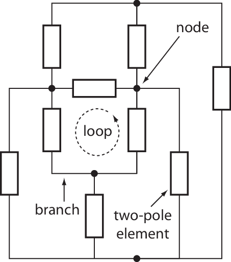
2.1.2 Dynamical variables of the circuit
The element of each branch at time is characterized by two variables: the voltage across the elements and the current flowing through it (see Fig. 5). For each branch we choose an orientation, arbitrary at this point, which will determine the sign of the current value. The voltage orientation is chosen to be opposite to that of the current for reasons that will become clear later.

The voltage and the current are defined from the underlying electromagnetic fields by
| (2.1) |
| (2.2) |
In Eq. 2.2 the loop integral is done along a closed curve in vacuum encircling the element.
Because we consider circuits in the lumped element approximation, these definitions make voltages and currents independent, to a large extent, of the precise path of integration along which fields are integrated. These paths are well outside the wire of inductors for the line integral of electric field (so that the magnetic field is zero along the path) and well outside the dielectric of capacitors for the loop integral of magnetic field (so the electric field is zero along the loop). Note that these definitions are sufficiently general to include the contribution to voltages of electro-motive forces due to time-varying magnetic fields and the contribution to currents of displacement currents due to time-varying electric fields. Note also that the factor in the definition of current comes from our choice of working with SI units throughout this review.
2.1.3 Energy absorbed by an element
The power absorbed by an element is given by the product of the voltage and current defined above (note the relevance of the sign convention here). We now introduce the total energy absorbed by an element :
| (2.3) |
In this expression the lower bound of the integral () refers actually to a time sufficiently far in the past that the circuit was completely at rest (This of course assumes the circuit contains a small amount of dissipation). An element is said to be purely “dispersive” (or “conservative”) if the energy is converted into stored electric or magnetic energy.
2.1.4 Generalized flux and charge associated with an element
An Hamiltonian description of electrical circuits requires the introduction of branch fluxes and branch charges which are defined from branch voltages and branch currents by
| (2.4) | |||||
| (2.5) |
As stated previously, the circuit is supposed to have been at rest at time with zero voltages and currents. Static bias fields imposed externally on the circuit such as magnetic fields through the inductors are supposed to have been switched on adiabatically from to the present.
2.1.5 Capacitive and inductive elements
A dispersive element for which the voltage is only a function of the charge and not directly of the time or any other variables, is said to be a capacitive element.
| (2.6) |
Its capacitance, which is only a function of the charge, is given by:
| (2.7) |
A linear capacitance has independent of and . One can easily compute that in this case .
Similarly, a dispersive element for which the current is only a function of the flux and not directly of the time or any other variables, is said to be an inductive element.
| (2.8) |
Its inductance, which is only a function of the flux, is given by:
| (2.9) |
A linear inductance has independent of and . One can easily compute that in this case .
As we have seen with Eq. 1.3, a Josephson tunnel junction possess a non-linear inductive element for which is a sine function: .
In summary, the energies of our three basic elements are given by the following table:
| Element | Energy |
|---|---|
| linear capacitance | |
| linear inductance | |
| Josephson element |
Let us stress that despite the presence of and in the expression of the energy of the Josephson element (through and ), it is at this stage a purely classical entity, which, from the point of view of collective variables like current and voltages, is on the same footing as a common inductance obtained by winding a piece of macroscopic wire. Universal quantum constants enter here only because the non-linear behavior of this element originates from the microscopic phenomenon of discrete electron tunneling events between the electrodes. Equations like Eqs. 2.6 and 2.8 are called the constitutive equations of the element.
A linear dispersive circuit consists only of linear capacitances and inductances, for example see Fig. 6.

2.1.6 Finding the degrees of freedom of an arbitrary conservative circuit
We suppose the circuit is sufficiently near rest that the constitutive equations can be linearized, i.e. the energy can be expanded as a quadratic term plus higher order corrections. The problem is now reduced to finding the degrees of freedom of the linear dispersive circuit corresponding to the quadratic term.
There are less degrees of freedom than there are branches in the circuits, since in addition to the constitutive relations, one has to take in to account Kirchhoff’s laws:
| (2.10) | |||||
| (2.11) |
One therefore has to eliminate superfluous variables. There exist two standard methods in circuit theory to achieve this goal: the method of nodes and the method of loops. Here we develop only the method of nodes which solves most practical problems. The two methods are dual to each other and the lessons learned in studying one of the them are easily transposed to the other.
Before examining the details of the method of nodes, one should first mentally divide the circuit into its capacitive sub-network and inductive sub-network. In the method of nodes we turn our attention away from the loops, which pose no problems, to face what happens at a node. Active nodes are defined as nodes in which inductances and capacitances meet. Passive nodes are where only capacitances or only inductances converge.
2.1.7 Method of nodes
In the method of nodes, we exploit the specificity of the capacitive sub-network to contain only linear elements. This is a reasonable assumption for the circuits we will be discussing. This assumption allows us to express the energy of a capacitance in terms of voltage, i.e. the derivative of flux. Inverting the constitutive relation given in Eq. 2.6, we can write the energy of a capacitive branch as . Thus in our treatment, we have broken the symmetry between charge and flux, and flux will play the role of “position”. With this choice inductive energy will be potential energy and capacitive energy will be kinetic energy.
We now proceed by explaining the technical details of the method of nodes. One first makes sure that at every node to which an inductance is connected, a capacitance is also connected. This does not need to be an artificial introduction, it corresponds to the always present parasitic capacitance of inductances. There are thus no passive nodes in the sub-network of inductances. On the other hand, it does not matter if this sub-network is not simply connected. In contrast, for the capacitive sub-network, we have to make sure it is simply connected. It can, however, have passive nodes. Thus, along with the symmetry between charges and fluxes, the symmetry between capacitances and inductances is broken in the method of nodes. We have thus ensured that every node is connected to any other node by a path involving only capacitances.
Listing all the nodes, the active nodes will be nodes to , while nodes to will be passive nodes of the capacitance sub-network. We first setup the inverse inductance matrix whose non-diagonal matrix elements are where is the value of the inductance connecting nodes and . Of course if there is no inductance between the nodes, which is true in particular for all passive nodes, the corresponding matrix element will be zero. The diagonal matrix elements will be the opposite of the sum of values in the corresponding row or column. We also introduce the capacitance matrix whose non-diagonal matrix elements are where is the capacitance connecting nodes and . The diagonal elements of the capacitance matrix are built similarly to that of the inductance matrix, by taking the opposite of the sum of values in the corresponding row or column.
What is the meaning of these matrices? Let us introduce the spanning tree of the capacitance sub-network. It consists of the choice of a particular active node called “ground” and the set of branches that connect the ground through capacitances to every other node, both active and passive, without forming any loops. There is thus only one path between the ground and every other node. For an example, see Fig. 7. This spanning tree allows us to assign a flux to each node by algebraically summing all the fluxes of the branches in the path between the ground and the node. We can now define the node flux column vector which has components. The choice of ground node and spanning tree is analogous to the choice of a particular gauge in electromagnetic field theory and to the choice of a system of position coordinates in classical mechanics.
These node flux are related to the branch fluxes by the relation:
| (2.12) | |||||
| (2.13) |
where is the set of spanning tree branches and is the complement of this set. The symbols and denote the nodes connected by the branch. The flux offset corresponds to the static flux that may be enclosed by a loop containing the branch.
We have defined the energy for each branch, and now we can express it using node fluxes. This leads to the equivalent of the potential energy of the circuit:
| (2.14) |
where the matrix differs from in that the row and column corresponding to the ground node have been eliminated. The second term sums over all the inductive branches of the circuit where and are the nodes connected by branch . If there is no inductor the term will be zero. The offset fluxes represent a strain of the inductance sub-network that is crucial to a wide range of phenomena involving Josephson junctions [21, 22, 23]. We will describe some of these effects later in the review.
The equivalent to the kinetic energy of the circuit is given by:
| (2.15) |
where the matrix differs from in that the row and column corresponding to the ground node have been eliminated. Note that there are no offsets in the kinetic energy term due to our choice of the tree to pass only through capacitances. The charge offset will appear later when we define the conjugate charges of node fluxes.

2.1.8 Setting up the Lagrangian
We can now obtain the Lagrangian by subtracting the potential energy from the kinetic energy . For the circuit of Fig. 6 and the choice of spanning tree of Fig. 7, one obtains the Lagrangian
| (2.16) | |||||
where the degrees of freedom and are the fluxes of the nodes and . One can check that by applying Lagrange’s equations
one recovers the correct equations of motion of the circuit. Our approach for the construction of the Lagrangian of a circuit generalizes the pioneering work of Yurke and Denker [24].
2.1.9 Conjugate variable pairs
From the Lagrangian, we can now define the momenta conjugate to the node fluxes, using the usual relation
| (2.17) |
It is important to note that, according to Lagrange’s equations, if is a passive node, since by our definition for all passive nodes in the capacitive sub-network. Thus, the circuit only has at most true degrees of freedom, corresponding to all the active nodes except the ground node. These new variables , which we call node charges, correspond to the algebraic sum of the charges on the capacitances connected to node . In the loop variable representation, the conjugate momentum of the loop charge is the sum of the fluxes in the inductors of the loop.
Note that Eq. 2.17 can be written in vector form as . It is possible to invert the capacitance matrix and thus express as a function of .
We can now find the normal modes of the circuit given by the eigenvectors of the matrix product associated with non-zero eigenvalues. The non-zero eigenvalues correspond to the normal mode frequencies of the circuit squared. There are thus at most normal mode, but symmetries in the circuit can reduce this number. We define the number of normal modes as . This number is equivalent to the number of independent equations generated by the Euler-Lagrange equations.
2.1.10 Finding the Hamiltonian of a circuit
The Hamiltonian can now be expressed as the sum of the kinetic energy, which is to be expressed in terms of the variable, and the potential energy expressed, as before, in terms of :
| (2.18) |
where the independent variables correspond to degrees of freedom, while the others correspond to offset charges. The potential energy is in general a non-linear function of the vector .
Taking again the example of the circuit of Fig. 6, we can apply this procedure and obtain the following Hamiltonian
| (2.19) | |||||
The first term in is the electrostatic energy of the circuit expressed as a function of the node charges, while the second term is the magnetic energy expressed as a function of node fluxes. This structure is a general characteristic of the Hamiltonian of a circuit in the node variable representation and does not depend on whether the elements are linear or not. The Hamiltonian formulation shows clearly the role of as an offset term in the magnetic energy. In the case of a linear inductor, the effect of this term is simply to induce an offset DC current. However, in the case of non-linear inductors like Josephson junctions, this term changes the dynamics of the circuit.
One can easily verify that Hamilton’s equations
| (2.20) | |||||
| (2.21) |
are equivalent to the equations of motion.
It is important to note that although the Hamiltonian of the circuit always gives its total energy, its functional form depends on the particular choice of spanning tree, even when the choice of a representation in terms of node variables or loop variables has been made.
However, the Poisson bracket [25] of the flux and charge of a branch is independent of the choice of the spanning tree and obeys:
| (2.22) |
where the value is for a capacitance and for an inductance. This important remark is far-reaching in the quantum case.
2.1.11 Mechanical analog of a circuit, does it always exist?
In the node variable representation, the node fluxes play the role of position coordinates and the node charges the role of momentum coordinates. The capacitive energy plays the role of the kinetic energy and the inductive energy plays the role of the potential energy. However, the form of the Hamiltonian of Eq. 2.19 with capacitive cross-terms shows that the particular circuit of Fig. 6 has no simple mechanical analog. In the cases where the capacitances are only connected between the active nodes and ground, they can be interpreted as the masses of the active nodes and a direct mechanical analog can be found for the circuit. The inductances then correspond to elastic coupling interactions between the masses associated with the nodes.
2.1.12 Generalization to non-linear circuits
It is remarkable that the formalism given above can be kept essentially intact when one goes to inductive elements with a polynomial expansion in branch fluxes. Special care must be taken, though, with the Josephson energy that is periodic in generalized flux. Also, when we deal with non-linear circuits, it is important that the capacitive sub-network remains linear. In the case of a linear inductive sub-network and a non-linear capacitive sub-network, we could resort to the method of loops. The case in which both inductive and capacitive sub-network are maximally non-linear is a subject of ongoing research.
2.2 Circuits with linear dissipative elements
2.2.1 The Caldeira-Leggett model
We would like now to treat circuits with linear dissipative elements like resistors. It would seem that the Hamiltonian formalism is powerless to treat a dissipative system, whose behavior is irreversible, since Hamilton’s equations of motion, Eqs. 2.20 and 2.21 are invariant upon time reversal. However, this reversibility problem can be solved by extending the formalism. This extension has in fact been made recurrently throughout the history of theoretical physics. We will present here a particular clear and useful version known as the Caldeira-Leggett model [1] which applies to systems with linear dissipation.
The essence of the Caldeira-Leggett model, in the context of electrical circuits, is to replace a linear dissipative two-pole characterized by a frequency dependent admittance by an infinite set of series LC oscillators all wired in parallel (see Fig. 8). The internal degrees of freedom of the admittance can be thought of as the fluxes of the intermediate nodes of the LC oscillators (open dots in Fig. 8). It is the passage from a finite number of degrees of freedom to an infinite one that reconciles the irreversible behavior on physical time scales and the formal reversibility of Hamilton’s equations of motion.


The reversibility problem appears when one notices that for every oscillator in the series, the admittance given by the usual combinatorial rules of circuit theory
| (2.23) |
is purely imaginary while the infinite series corresponding to has both a real and imaginary part (we use here the symbol
| (2.24) |
of electrical engineers but with an opposite value to ensure later compatibility with the sign convention of quantum mechanics concerning Fourier transforms). This manifestation of the reversibility problem disappears by extending the notion of admittance function to complex frequencies.
Let us recall that is defined from the relationship between the voltage across a linear element and the current flowing across it
| (2.25) |
| (2.26) |
We can define an extension of by the relation
| (2.27) |
(there is no problem at since is a causal function).
All information on the shape of after is erased in . Let us now define the generalized admittance function by
| (2.28) |
We find that the generalized admittance of the m-th LC circuit in the Caldeira-Leggett model is given by
| (2.29) | |||||
where and are the resonant frequency and impedance of the m-th oscillator. It has both a real and a imaginary part. The idea of Caldeira and Leggett thus consists in replacing the smooth function by an infinitely dense comb of functions. Mathematically this corresponds to the following relations between and the series of oscillators with finite frequency:
| (2.30) | |||||
| (2.31) | |||||
| (2.32) | |||||
| (2.33) |
Note that if the admittance corresponds to a pure conductance, all the elements have the same value. In order to properly treat the response of the admittance at zero frequency, we have to introduce a 0-th element consisting only of an inductance , with the conjugate capacitance being reduced to a short circuit ().
| (2.34) |
Knowing the infinite set of elements, the full admittance function can be expressed as
| (2.35) |
It is important to note that the Caldeira-Leggett model does not constitute a representation of the internal workings of a dissipative element. It should be used only to calculate the influence that such an element will have in the dynamics of the collective variables of the circuit. We calculate this influence by adding to the Hamiltonian of the rest of the circuit the Hamiltonian of the admittance
| (2.36) |
This Hamiltonian has been written in the node representation where the ground has been chosen on one terminal of the admittance. The node flux corresponds to the other terminal of the admittance while the node fluxes correspond to the intermediate nodes of the LC oscillators. The charge on the capacitances are the momenta conjugate to . It is useful to note that the coupling between the admittance and the circuit it is connected to is of the gauge form: the coupling term in implicitly contained in the displacement of by the main flux .
2.2.1.1 Voltage and current sources
Constant sources of voltages and current can also be treated by the Hamiltonian formalism. A voltage source can be represented as a divergingly large capacitor in which is stored initially a large charge such that in the limit . Likewise, a current source can be seen represented by a divergingly large inductor in which is stored initially a large flux such that in the limit . Alternating voltage and current sources can, in the same manner, be treated using pre-excited LC oscillators.
2.2.2 Fluctuation-dissipation theorem
The value of the Caldeira-Leggett model becomes apparent when we use it to derive the fluctuation-dissipation theorem. Suppose that the admittance , which we suppose in thermal equilibrium at temperature , is short-circuited. In that case the variable in the Hamiltonian (2.36) is identically zero and all the oscillators become independent. The current through the short is zero on average but will fluctuate. We can easily calculate the spectral density of these fluctuations by setting to the value of each energy term in the Hamiltonian (2.36). For each oscillator we can obtain the correlation function of the charge on the capacitance
| (2.37) |
The correlation function of the current through the oscillator is therefore
| (2.38) |
Using the relation in Eq. 2.29 we can rewrite this relation as
| (2.39) |
Since all the oscillators are independent, we can add their correlation functions to obtain the correlation of the current through the short
| (2.40) |
and thus
| (2.41) |
We finally obtain the spectral density of current fluctuations in equilibrium defined by
| (2.42) |
in terms of the impedance function (Nyquist theorem)
| (2.43) |
The spectral density of thermal equilibrium voltage fluctuations across a linear dissipative element can be obtained as a function of its impedance in a similar manner. Using the Caldeira-Leggett representation of an impedance (see Fig. 9)
| (2.44) |
3 Hamiltonian Description of the Quantum Dynamics of Electromagnetic Circuits
3.1 Non-dissipative quantum circuits
3.1.1 From variables to operators
The passage from the classical to the quantum description of electrical circuit is straightforward in the framework of the Hamiltonian description developed in the preceding section. The classical variables are replaced by corresponding operators and the Hamiltonian function is replaced by a function of operators:
| (3.1) |
The state of the circuit is likewise represented by the density operator, which lives in the Hilbert space dual to that of the Hamiltonian.
3.1.2 Commutators of charge and flux
The operators corresponding to the position coordinates, here node fluxes, all commute. However, pairs of operators corresponding to conjugate variables do not commute. In the node variable framework, the commutator of the node fluxes and their conjugate node charges is:
| (3.2) |
This relation stems from the quantization of the electromagnetic field and corresponds to the fundamental commutator for conjugate variables. Of course, Eq. 3.2 is valid only if the electric state of node is a true degree of freedom of the circuit, meaning that neither , or their derivatives are constants of motion. More generally, as shown by Dirac [26], the value of a classical Poisson bracket imposes the value of the corresponding commutator
| (3.3) |
It follows from Eq. 2.22 that the flux and the charge of a branch have the commutator
| (3.4) |
where the sign depends on the branch being capacitive or inductive.
Note, however, that in general these branch operators are not conjugate operators in the Hamiltonian. This stresses the importance of finding the correct degrees of freedom of the circuit, which can then be quantized.
3.1.3 Useful relations
Usual relations of quantum mechanics can be adapted to electrical systems. For an arbitrary operator we have:
| (3.5) | |||||
| (3.6) | |||||
| (3.7) |
The sign of the right-hand side in these relations can be obtained by matching the order of the variables on the left-hand side to the order of variables in the columns of the following mnemonic table:
The integral form of these relations will also be useful:
| (3.8) |
| (3.9) | |||||
| (3.10) |
In order to simplify notations, the hats on operators will be dropped from now on. We will of course make sure that the distinction between operators and c-numbers can be made from the context.
3.1.4 Representations of the Hamiltonian and canonical transformations
3.1.4.1 The quantum LC oscillator
The LC oscillator of Fig. 1 can now be treated quantum mechanically. This circuit with only one active node has a trivial topology. We can immediately adapt well-known textbook results on the harmonic oscillator. Taking as variables the integral of the voltage across the inductor and the corresponding charge on the capacitor we have the Hamiltonian
| (3.11) |
Introducing the usual annihilation and creation operators such that
| (3.12) |
we have
| (3.13) | |||||
| (3.14) |
| (3.15) |
where, as in section 1,
| (3.16) |
and where
| (3.17) |
represent the standard deviations of the flux and charge fluctuations of the ground state, respectively. Using Eq. 3.8 and the relation
| (3.18) |
where , we can calculate the flux-flux correlation function in thermal equilibrium . We arrive at
| (3.19) |
and from
| (3.20) |
we get finally
| (3.21) |
Setting , we get the variance of flux fluctuations at temperature
| (3.22) |
which interpolates between the zero-point fluctuations result and the high temperature result .
From we also get the variance of charge fluctuations
| (3.23) |
An important remark can be made: Not only does Eq. 3.21 predict that the amplitude of fluctuations saturates at low temperature (well-known zero-point fluctuations) but it also predicts that the quantum correlation function is not real! The Fourier transform of the correlation function thus cannot be interpreted as a directly measurable spectral density as it is the case classically. Let us now discuss the case of a general impedance to further examine this point.
Introducing the generalized impedance function of an LC oscillator
| (3.24) | |||||
we can rewrite Eq. 3.21 as
| (3.25) |
3.2 Dissipative quantum circuits
3.2.1 The quantum fluctuation-dissipation theorem
We can now obtain the quantum correlation function of the branch flux across an arbitrary generalized impedance by using the Caldeira-Leggett representation of Fig. 10. We simply add the contribution of all the oscillators and since the correlation function is a linear function of the real part of the impedance we directly obtain a result of central importance:
| (3.26) |
If we now introduce the spectral density of quantum fluctuations
| (3.27) |
we get the frequency domain relation
| (3.28) |
which is also called the quantum fluctuation dissipation theorem [27]. Note again that in contrast with a classical spectral density of fluctuations . The square brackets have a new meaning here, indicating that both positive and negative frequency arguments have each a separate role, as explained below.
How should we interpret ? To make easier the comparison with the classical case let us calculate the voltage-voltage spectral density
| (3.29) |
which is related to by
| (3.30) |
In the various limits of interest, is given by
|
|
(3.31) |
3.2.1.1 Interpretation of the quantum spectral density
The form of in the quantum limit shows that the part of quantum spectral densities correspond to processes during which a “photon” is transferred from the impedance to the rest of the circuit while the part corresponds to the reverse process. The quantum fluctuation-dissipation theorem constitutes a generalization of Planck’s black body radiator law. The impedance plays the role of the black body radiator while the rest of the circuit plays the role of the atom. Finally, the and processes correspond to absorption and emission processes respectively. Note that for the part of corresponds to spontaneous emission.
3.2.1.2 Quantum fluctuations in the damped LC oscillator
How does dissipation modify the results of Eqs. 3.22 and 3.23? We can apply the quantum fluctuation-dissipation theorem to compute the fluctuations of the damped LC oscillator of Fig. 1b. This system can be represented by the circuit diagram of Fig. 10 in which we have replaced the admittance shunting the main LC oscillator by an infinite set of series LC oscillators in parallel.

| (3.32) |
Since this Hamiltonian is quadratic we can in principle find its normal mode coordinates. However, there is a more efficient method. We can treat the circuit taken between ground and the closed dot in Fig. 10 as a dissipative element with an impedance given by
| (3.33) |
Taking the spanning tree to go through the main inductance the node flux is identical to the flux through that inductance and we get
| (3.34) |
Similarly, the conjugate charge is identical to the charge on the main capacitance and we have
| (3.35) |
We can now apply these results to the so-called Ohmic case (or resistor case) where the damping admittance is independent of frequency below a cutoff frequency which we take to be much larger than . We take of the form
| (3.36) |
The integrals in Eqs. 3.34 and 3.35 can be calculated in closed form [28] and one finds that in the limit , becomes independent of . We have
| (3.37) |
where is the polygamma function and
| (3.38) |
| (3.39) |
| (3.40) |
In contrast with , diverges as , a specifically quantum mechanical result. We have
| (3.41) |
where
| (3.42) |
| (3.43) |


3.2.1.3 Low temperature limit
In the limit we find the analytical expressions
| (3.44) |
| (3.45) |
It is interesting to calculate how the quantum fluctuations depend on the damping coefficient in the limit
| (3.46) | |||||
| (3.47) |
We find that the surface of the uncertainty ellipse grows logarithmically with damping
| (3.48) |
an effect due to the presence of quantum degrees of freedom inside the resistor. Apart from that feature, we note that the effect of a resistor on the quantum mechanical fluctuations of the LC oscillator is essentially to rescale the size of these fluctuations. We will see in the next section that the non-linear oscillator formed by a Josephson junction can have a qualitatively distinct behavior.
3.2.2 Input-Output theory
We now present an alternate theory of the damping of a quantum circuit by a dissipative environment. It is based on a role reversal: instead of considering that the circuit loses and gains energy from the environment, we can view the circuit as an elastic scatterer of signals coming from the environment. This approach, nicknamed “input-output theory”, has the merit of placing the external drive and dissipation of the circuit on the same footing and offers a deeper understanding of the fluctuation dissipation theorem. On the other hand, it simplifies the analysis in the case where the oscillations of the circuit are well within the under-damped regime. This condition makes the environment appear like a resistance (white noise) in the relevant frequency range. This part of the review follows the appendix of Ref. [29] which is itself based on the book by Gardiner and Zoller [30].

3.2.2.1 Infinite transmission line
Input output theory is based on the Nyquist model of the dissipation by a resistance, in which the environment as replaced by a semi-infinite transmission line (See. Fig. 13). Before we treat the coupling between the circuit and this semi-infinite transmission line, let us review the quantization of the field traveling along an infinite transmission line.
The capacitance and inductance per unit length of the line are and , respectively. The equations obeyed by the current along and the voltage across the line are
| (3.49) | ||||
| (3.50) |
in which, for the moment, we treat the fields classically. The characteristic impedance and propagation velocity are given by
| (3.51) | ||||
| (3.52) |
In order to solve Eqs. 3.49) and 3.50), we introduce two new fields: the left-moving and right-moving wave amplitudes,
| (3.53) | ||||
| (3.54) |
which have the advantage of treating currents and voltage on the same footing (note that these amplitudes are not directly related to the vector potential). The dimension of these fields is [watt]1/2 and they are normalized such that the total power traversing, in the forward direction, a subsection of the line at position and time is given by
| (3.55) |
The quantity here plays the role of the Poynting vector in full 3D electrodynamics. Each of the terms at the right hand side of the last equation is thus the separate contribution of the corresponding wave to the total power flow.
When solving Eqs. 3.49 and 3.50, we find
| (3.56) |
This relation means that does not depend separately on or but a combination of both and thus:
The properties of the wave amplitude can be summarized by writing
| (3.58) | ||||
| (3.59) | ||||
| (3.60) |
Note that the detailed definition of the retardation depends on the wave direction. We now turn to the energy density , related to by the local energy conservation law
| (3.61) |
Combining Eqs. 3.55 and 3.56, we get
| (3.62) |
The total energy of the line at time is, thus,
| (3.63) |
When in Eq. 3.63 is considered as a functional of dynamical field variables and , the equation of motion Eq. 3.56 can be recovered from Hamilton’s equation of motion as
| (3.64) |
on imposing the Poisson bracket
| (3.65) |
Therefore, from the classical-quantum correspondence involving the replacement of Poisson brackets by commutators, we find that the quantum operator version of the fields satisfy the commutation relation
| (3.66) |
which is analogous to the commutation relation between the electric and magnetic field in 3-D quantum electrodynamics. Note that the fields are Hermitian at this stage. Introducing the Fourier transform for signals (whose normalization differs from the previously introduced Fourier transform for response functions),
| (3.67) |
where the Fourier components (which are now non-Hermitian operators) satisfy
| (3.68) |
we can also write the Hamiltonian as
| (3.69) |
The field operators in the frequency domain satisfy
| (3.70) |
We now introduce the usual quantum field annihilation operators
| (3.71) | ||||
| (3.72) |
They satisfy the commutation relations
| (3.73) |
It is useful to note that since
| (3.74) |
Eq. 3.73 exhaustively describes all possible commutator cases.
In the thermal state of the line, at arbitrary temperature (including ),
| (3.75) |
where
| (3.76) |
These last two equations can be seen as a consequence of the Wiener-Kinchin theorem, and are explained in detail in ref. [31]. When is strictly positive is the number of available photons per unit bandwidth per unit time traveling on the line in a given direction around frequency
| (3.77) | ||||
| (3.78) |
Positive frequencies correspond to the line emitting a photon, while negative frequencies correspond to the line receiving a photon.
| (3.79) |
The Bose-Einstein expression is expected from the Hamiltonian of the line, which reads, with the operators,
| (3.80) |
We can now give the expression for the anticommutator of the fields
| (3.81) |
When external drives are present, Eq. 3.81 has to be modified with an additional term:
| (3.82) | ||||
| (3.83) |
We now introduce the forward-propagating and backward-propagating voltage and current amplitudes obeying
| (3.84) | ||||
| (3.85) |
| (3.86) | ||||
| (3.87) |
Quantum-mechanically, the voltage and current amplitudes become hermitian operators
| (3.88) | ||||
| (3.89) |
These operators, in turn, can be expressed in terms of field annihilation operators as
| (3.90) | ||||
| (3.91) |
All physical operators can be deduced from these primary expressions. For instance, the transmission line charge operator, describing the charge in the line brought from one end to the position , is
| (3.92) |
3.2.2.2 Nyquist model of resistance: semi-infinite transmission line
We now are in a position to deal with the semi-infinite line extending from to , whose terminals at models a resistance [see Fig. 13]. In that half-line, the left- and right-moving propagating waves are no longer independent. We will now refer to the wave amplitude as and as . The quantum-mechanical voltage across the terminal of the resistance and the current flowing into it satisfy the operator relations
| (3.93) | ||||
| (3.94) |
These relations can be seen either as continuity equations at the interface between the damped circuit and the resistance/line, or as boundary conditions linking the semi-infinite line quantum fields and . From the transmission line relations,
| (3.95) |
we obtain
| (3.96) | ||||
| (3.97) |
For a dissipationless circuit with Hamiltonian , where is the generalized flux of the node electrically connected to the transmission line, and its canonically conjugate operator (top panel of Fig. 13, we can write the Langevin equation,
| (3.98) |
The latter equation is just a particular case of the more general quantum Langevin equation giving the time evolution of any operator of a system with Hamiltonian , which is coupled to the semi-infinite transmission line by an Hamiltonian term proportional to another system operator ,
| (3.99) | ||||
The value of in Eq.3.99 depends on whether the damping is “parallel” () or “series” type () [see Fig. 13]. In the parallel case, the greater the line impedance the smaller the damping, whereas in the series case the situation is reversed.
Equation 3.99 should be supplemented by
| (3.100) |
and
| (3.101) |
It follows from the last three equations that the output fields have the same commutation relation as the input fields
| (3.102) |
3.2.2.3 Quantum Langevin equation in the rotating wave approximation
We now consider an approximate form of the input-output formalism which is only valid when the system degree of freedom consists of an oscillator with very low damping, and for which all the frequencies of interest will lie in a narrow range around the oscillator frequency . We start from Eq. 3.98 and use
| (3.103) | ||||
| (3.104) |
where and .
We then obtain, neglecting the effect of driving terms oscillating at twice the resonance frequency,
| (3.105) |
with
| (3.106) |
The field amplitude is non-Hermitian and contains only the negative frequency component of . For signals in a narrow band of frequencies around the resonance frequency, we can make the substitution
| (3.107) |
where the frequency components of are equal, in the vicinity of , to those of the input field operator , itself identical to of the infinite line. We finally arrive at the RWA quantum Langevin equation, also referred to in the quantum optics literature as the quantum Langevin equation in the Markov approximation
| (3.108) |
where
| (3.109) |
For any oscillator, the input output relationship is obtained from
| (3.110) |
It is worth noting that although and play the role of and in Eq. 3.73, only the average values of the moments of can be imposed, being a “slave” of the dynamics of , as processed by the oscillator.
3.3 Measurement operators
We now introduce the notion that the environment is not completely passive but is able to collect information coming from the system damped by the environment. All quantum measurement experiments on single systems can be analyzed within this framework. Thus, we replace the semi-infinite transmission line of the preceding subsection by a finite transmission terminated by an absorptive detector. This detector performs, of course, measurements on the traveling electromagnetic signal but we can refer its actions to the system itself through Eq. 3.110.
In practice, there are three types of measurement that can be performed:
- 1.
Homodyne measurement, in which the system degree of freedom is analyzed along one component in phase space (i.e. ). Eigenstates of such measurement satisfy a relation of the form where is the in-phase component of the oscillator, analogous to the position.
- 2.
Heterodyne measurement, in which the system degree of freedom is analyzed along two orthogonal components in phase space (i.e. ). In this type of measurement two conjugate operators are measured simultaneously, which necessarily results in added noise. Eigenstates of such measurement satisfy a relation of the form where is a complex number and is a coherent state. Note that these eigenstates form an over-complete basis, which is another direct result of the commutation relation between two conjugate operators.
- 3.
Photon measurement, in which the system degree of freedom is analyzed in terms of the excitation quanta (i.e. ). Eigenstates of such a measurement satisfy a relation of the form where is a Fock state with photons.
3.3.1 The stochastic master equation
So far, we have discussed the evolution of the quantum circuit under the influence of the Hamiltonian and an external environment interacting with it. We have done this in the operator language, but it is also useful to recast this theory in the language of the density matrix. This leads to the stochastic master equation [32, 33], which describes the evolution of the density conditioned by the succession of measurement outcomes, also known as the measurement record. An advantage of this formalism is that we end up with an ordinary differential equation in complex number with no non-commuting variables.
The stochastic master equation can be divided into three parts: the first is the Hamiltonian evolution which is the usual Schrödinger equation, analogous to the Heisenberg equation part of the quantum Langevin equation (Eq. 3.108). The second is the Lindblad dissipative evolution, analogous to decay term in the same equation. The last part is the measurement back-action, which corresponds to the stochastic perturbation of the system by a measurement. This term corresponds in the quantum Langevin equation to the influence of the input field. In this formalism, the fluctuation-dissipation theorem is exhibited by the relationship between the back-action of the measurement and the decay of the system.
4 Superconducting Artificial Atoms
4.1 The Josephson element
4.1.1 The energy operator for the Josephson element
As we have seen in the introduction, a superconducting tunnel junction can be modeled by a pure tunnel element (Josephson element) in parallel with a capacitance. The Josephson element is a pure nonlinear inductance and has an energy operator function of the branch flux given by
| (4.1) |
where is the reduced flux quantum and is an offset branch flux whose role will be discussed later. For the moment suffice to say that its meaning is such that the energy of the element is minimum for . In the following we introduce the so-called gauge invariant phase difference . The justification of this inductive energy operator is the following: Consider two isolated superconducting electrodes separated by a thin oxide layer. The electrodes have a number of Cooper pairs and respectively. While the sum is conserved, the difference is the degree of freedom of the Cooper-pair tunneling process.
Quantum-mechanically, should be treated as an operator whose eigenstates are macroscopic states of the two electrodes corresponding to a well-defined number of Cooper pairs having passed through the junction
| (4.2) |
One can show that the tunneling of electrons through the barrier couples the states [34]. The coupling Hamiltonian is
| (4.3) |
The Josephson energy is a macroscopic parameter whose value for BCS superconductors on both sides of the junction is given by [3]
| (4.4) |
where is the superconducting gap and the tunnel conductance in the normal state. The tunnel conductance is proportional to the transparency of the barrier and to the surface of the junction.
In the next subsection we are going to show that and correspond to two representations of the same physical energy.
4.1.2 The phase difference operator
Let us now introduce new basis states defined by
| (4.5) |
The index should be thought as the position of a point on the unit circle since
| (4.6) |
leaves unaffected.
We have conversely
| (4.7) |
from which we can obtain the expression of in the basis
| (4.8) |
It is natural to introduce the operator
| (4.9) |
which is such that
| (4.10) |
We can thus write the coupling Hamiltonian (4.3) as
| (4.11) |
Thus, if we identify with , and represent the same Hamiltonian. Note that , as a reduced generalized flux, a pure electromagnetic quantity, takes its values on the whole set of real numbers, whereas is an angle taking its values on the unit circle. While one might think that and bears close resemblance to the couple formed by the number and phase operators for a mode of the electromagnetic field in quantum optics, it should be stressed that here the pair number operator takes its eigenvalues in the set of all integers, positive and negative, whereas the number of photons takes its values in the set of non-negative integers only. We can write symbolically
| (4.12) |
being aware of the fact that due to the compact topology of the manifold , only periodic functions of like have a non-ambiguous meaning.
| (4.13) |
Since couples linearly to the voltage operator via the charge involved in Cooper-pair transfer, we have
| (4.14) |
In the last equation we have used the identity .
Using the same type of algebra as in Eqs 4.13 and 4.11, we find that the current operator is given by
| (4.15) |
where
| (4.16) |
4.1.3 Loop combination of several Josephson elements (or a loop formed by a linear inductance and a Josephson element)
Let us return to the role of the parameter. One could think that it is a fully inconsequential quantity just like the position of the origin of a coordinate system. However, its role appears as soon we have a loop of several inductances, one of which at least being a nonlinear element, such as a Josephson junction. We now introduce the externally imposed flux threading the loop. From Faraday’s law, we have and thus
| (4.17) |
Eq. 4.17 indicates that around a loop the reduced flux will be in general different from zero, and tunable by the external flux. Thus, the external flux introduces frustration in the system, as not all branches can now have minimal energy. The experimentally observable zero frustration will be obtained when . Therefore, the sum around a loop of the offset fluxes is observable even though each branch value is not.
Adjusting the frustration in the system by an external flux is crucial in all loop-based quantum circuits, and here we will treat two classic examples.
4.1.3.1 Junctions in parallel: The DC SQUID
The circuit nicknamed “DC SQUID” consists of two Josephson tunnel junctions in parallel forming a loop threaded by a flux . We neglect here the linear inductance of the loop wire. The total inductive energy of this device is
| (4.18) |
Where and are the respective Josephson energies of the two junctions, and and are the phases across them. Due to the loop, the phases are related by . Using trigonometric identities, we can recast the equation to a single cosine
| (4.19) |
Where , and the new degree of freedom is . Note that this device behaves identically to a single junction, with a tunable Josephson energy. Note also that the offset flux in the definition of changes with the external flux if the junctions are not identical, but this effect is not directly observable unless the DC SQUID itself is part of a loop.
While the phase potential of the DC SQUID has only even powers of for any asymmetric and flux, a variation of the asymmetric DC SQUID in which we replace one of the junctions by two larger junctions in series does not have this even symmetry. This circuit is known as the flux qubit (see below). Note that for the right combination of the ratio between the small and large junction and external flux, one can null out the term in the phase potential while maintaining a nonzero term. This property is useful for making a pure three-wave-mixing device.
4.1.3.2 Junctions in series: Josephson junction arrays
Let us now consider an array of identical Josephson junctions in series, each with Josephson energy . Let us suppose also that the total reduced across the array is split equally among the junctions. This hypothesis corresponds to neglecting the effect of the capacitances across the junction, which would allow the current through the Josephson elements to split-off in the array of capacitances. The total energy can thus be written as
| (4.20) |
This equation is strictly valid only when the capacitance array meets two conditions. The capacitance across each junction allows phase slips across it () and therefore must be such that the phase-slip exponential factor [35, 36] where is the Coulomb charging energy of the junction. The other condition stipulates that the capacitance between the array islands and the ground must satisfy in order to make the self-resonance of the array above the junction plasma frequency .
In the limit where this Hamiltonian tends towards
| (4.21) |
which is the Hamiltonian of a linear inductance whose value is . This allows us to make superinductances, i.e. inductances whose impedances at frequencies below the self resonant frequency are well above the resistance quantum , which is impossible with ordinary geometric inductance[37].
4.2 Electromagnetic quantum circuit families
In this subsection we present a variety of electromagnetic quantum circuits which address various parameter regimes. The different circuits can be distinguished using the two dimension-less ratios and , where the electrostatic energy which now includes the total capacitance shunting the junction, and is the inductive energy due to an inductance shunting the junction.
The first ratio can be understood as the “mass” parameter of the Josephson junction. For the charge having passed through the junction is a good quantum number, and the Cooper-pair tunneling caused by the junction is a small effect. For the phase of the junction is a good quantum number and we can expand the phase energy, which we think of as a potential energy, around its minimum value. Thus, the capacitive energy takes the role of the kinetic energy. In this regime one can compute the standard deviation of the phase fluctuations .
The second ratio can be understood as being approximately the number of wells minus one in the phase potential, at . The useful circuits are always such that this ratio is positive, which means there are always at least two well at half a flux quantum. This corresponds to the classical potential supporting hysteretic minima.
In Table 1 we present the different circuits and their place in the circuit “periodic table” given by the two ratios described above. We also give a little map (see Fig. 14) in parameter space of the different problems plaguing the performance of quantum circuits in the current state-of-the-art.
| 1 | |||||
| cooper-pair box | |||||
| quantronium | fluxonium | ||||
| transmon | flux qubit | ||||
| phase qubit | |||||

4.2.1 Flux noise and charge noise
To understand this map let us write the Hamiltonian for our three element basic circuit including the influence of noise:
| (4.22) |
Here is the conjugate to which satisfies and and describe the charge and flux noise respectively. Let us point out that , unlike introduced before, is not the integer number of Cooper pairs having traversed the junction but the charge on the capacitance in units of . In the last term of Eq. 4.22, the combination can be understood as the total flux threading loop formed by the inductor and the Josephson element.
Let us first treat the case , then one can perform a gauge transformation where , which leads to the new Hamiltonian:
| (4.23) |
where is the time derivative of . Thus we transformed charge noise into offset flux noise. To the usual flux noise influence, we must now add a term related to . The expression for the effect of flux and charge fluctuations on qubit coherence can now be expressed as
| (4.24) |
Note that since we are now sensitive to current instead of charge fluctuations, we suppress low frequency charge noise by the factor [39]. This is equivalent to the idea the inductance shunts the charge fluctuations. Notice however, that this suppression is weighted by at the denominator, and so as the shunting inductance increases, the effect of charge noise can become dominant.
It is now apparent why is a special case. In this regime we are completely insensitive to flux noise, but we remain sensitive to charge noise through the expression
| (4.25) |
This sensitivity to charge noise can be reduced exponentially by reducing the value of , while losing nonlinearity only linearly [40].
4.2.2 The Cooper pair box
The Cooper pair box consists simply of a “small” Josephson junction () with no shunt inductance, and for which the offset charge can be controlled by an external gate voltage. For most of the gate voltage range, the energy eigenstates of this circuit are eigenstates of since the charging Coulomb energy dominates the Hamiltonian. However, at the special points the degeneracy between and is lifted by the Josephson energy, resulting in a pseudo-spin with Zeeman energy [41]. The Cooper pair box is the first quantum circuit in which Rabi oscillations between the ground and first excited state have been observed [42].
4.2.3 The transmon
The transmon [40] qubit is a Cooper pair box (with Josephson energy and capacitance ) shunted by a large capacitance . The capacitances are added into the total capacitance , so that the electrostatic energy is significantly reduced ().
The significant benefit of reducing the capacitive energy is removing the sensitivity of the qubit frequency to charge noise. A drift in the charge offset across the junction is screened by the capacitance and no longer changes the transition frequency between the ground and first excited state of the device, thus leading to higher coherence times.
4.2.4 The flux qubit
The flux qubit [43] is derived from the original proposal by A. J. Leggett of observing macroscopic quantum coherence oscillations between flux states of the RF-SQUID [44, 2]. Instead of the RF-SQUID, which consists of a Josephson junction shunted by a geometric inductance, the flux qubit consists of a Josephson junction shunted by an effective inductance made up of an array of several bigger Josephson junctions in series (see “Josephson junction arrays” above).
For most external flux bias values, the ground state adopted by the system is an eigenstate of the current in the loop and the inductive energy of the circuit (last two terms in Eq. 4.22). At exactly there are two degenerate current states for the device, corresponding to two wells in the potential. This degeneracy is lifted by the Coulomb charging term. The ground-excited state transition energy is a sensitive function of both and .
The coherence time of the flux qubit is significantly reduced when moving even slightly away from the optimal flux point, due to the high sensitivity of the qubit to flux qubit. To decrease this sensitivity, a variant of the flux qubit [45] has been proposed in which its ratio is reduced. While decreasing the sensitivity to flux noise, this qubit is now more sensitive to charge noise. To decrease this dependence, a large capacitance is added in parallel with the junction (similar to the transmon qubit), and so this qubit is often called the C-shunt flux qubit [46].
4.2.5 The phase qubit
The phase qubit [47] is derived from the device on which the first observations of macroscopic quantum energy levels were performed by exploiting the phenomenon of macroscopic quantum tunneling [48]. However, in this qubit the state measurement is performed using flux detection by a DC-SQUID rather than detection of a DC voltage by a low-noise semiconductor amplifier. It consists of a large Josephson junction shunted by a geometric inductance, biased to have a metastable potential well. In contrast with other qubits, the Hilbert space for the phase qubit is destroyed by the measurement as the phase particle leaves the metastable well.
The merit of this qubit is that the signal-to-noise ratio in the readout signal is very high due to the macroscopic tunneling effect.
4.2.6 The fluxonium
The fluxonium [49] artificial atom is a loop circuit made up of a small Josephson junction (with Josephson energy and Coulomb energy ) in parallel with a large linear inductor, meaning that its inductive energy satisfies . The presence of the inductor suppresses the DC component of offset noise as it shunts the two sides of the junction.
However, a large physical inductance, for example a wire of finite length , is always accompanied by a parasitic capacitance . This leads to a - oscillator mode that should not shunt the phase fluctuations of the junction. We thus need to satisfy where is the resistance quantum. This is impossible to achieve with a geometrical inductance, as its characteristic impedance will always be limited by the vacuum impedance of . Instead, the fluxonium inductance is implemented using an array of large Josephson junctions (see “Josephson junction arrays” above).
The fluxonium level structure strongly depends on the external flux across its loop, and this device can be considered a different artificial atom at every flux point. At the low energy fluxonium states are localized inside a single well in flux, and its first excitations are plasma excitation - resembling those of the transmon. At the fluxonium low energy states are in two flux wells simultaneously, similar to those of the flux qubit. These are the “sweet spots” of the fluxonium, where its energy is first-order insensitive to noise in the external flux and thus the dephasing is minimal.
5 Conclusions and Perspectives
The basic concepts of quantum circuits have been discussed in this review. First, a link has been established between standard Quantum Electrodynamics, which deals with how electrons and photons interact in the vacuum, and Josephson circuits in the quantum regime, in which the degrees of freedom are not associated to microscopic particles, but to collective variables of electronic condensed phases of matter which, at low temperatures, can have only a few excitations. The circuit linear inductances and capacitances form a medium analogous to that of the vacuum supporting the electric and magnetic fields in QED while the role of the Josephson junction corresponds to the non-linear interaction process between electrons and photons. Second, the open system character of quantum circuits has been introduced and we have explained how dissipation of resistances can be dealt with within a quantum-mechanical context. Finally, we have reviewed several examples of key basic circuits and examined the role played by noises in the decoherence of the qubits that can be implemented in these circuits.
Several important topics have been left outside the scope of this review. In particular, the endeavor consisting in using Bloch oscillations at the metrological level has been completely glanced over [50]. In this type of quantum physics, the roles of flux and charge are completely interchanged with respect to their role in commonly used circuits like the transmon. Linked to the question of Bloch oscillation are the proposals of circuits with topological protection from decoherence [51, 52]. Another fundamental topic of interest, that of driven-dissipative circuits, has also been excluded. In the present review, circuits have been considered as passive devices since no energy was provided to power them. A whole new paradigm is opened when a quantum circuit is submitted to drives at microwave frequencies, which seed the circuit with a bath of photons that can can nourish weak probe signals and dress-up the bare Hamiltonian, giving it entirely new functionalities. We believe that several of these rich topics will yield important discoveries in the near future, keeping the field of quantum circuits as exciting as when the present review was finished!
Acknowledgements
The authors are indebted to many colleagues for useful discussions. In particular, we would like to thank Baleegh Abdo, Steven Girvin, Michael Hatridge, Archana Kamal, Angela Kou, Zaki Leghtas, Zlatko Minev, Mazyar Mirrahimi, Ananda Roy, Daniel Sank, Robert Schoelkopf, Shyam Shankar, Clarke Smith, and Evan Zalys-Geller. This work was supported by ARO under Grant No. W911NF-14-1-0011, by MURI-ONR Grant No. N00014-16-1-2270 and by MURI-AFOSR Grand No. FA9550-15-1-0029.
References
- [1] A. O. Caldeira and A. J. Leggett, “Quantum tunnelling in a dissipative system,” Annals of Physics, vol. 149, no. 2, pp. 374–456, 1983.
- [2] A. Leggett, Quantum mechanics at the macroscopic level, in “Chance and Matter”. North Holland, 1987.
- [3] B. Josephson, “Possible new effects in superconductive tunnelling,” Physics Letters, vol. 1, no. 7, pp. 251–253, 1962. Note that the value of calculated for the first time by Josephson - he calls this parameter in his original article - is greater by a factor of 2 than the correct value later found by Ambegaokar and Baratoff (with contribution by DeGennes).
- [4] B. D. Josephson, in ”Superconductivity”. Marcel Dekker, 1969.
- [5] S. Haroche and J.-M. Raimond, Exploring the Quantum: Atoms, Cavities and Photons. Oxford University Press, Oxford, 2006.
- [6] A. Blais, R.-S. Huang, A. Wallraff, S. M. Girvin, and R. J. Schoelkopf, “Cavity quantum electrodynamics for superconducting electrical circuits: An architecture for quantum computation,” Phys. Rev. A, vol. 69, p. 062320, Jun 2004.
- [7] H. Grabert and M. Devoret, eds., Single Charge Tunneling. Plenum, New York, 1992.
- [8] R. P. Feynman, Lectures on Physics, vol. 2. Addison-Wesley, 1964.
- [9] M. A. Nielsen and I. L. Chuang, Quantum Computation and Quantum Information. Cambridge University Press, Cambridge, 2000.
- [10] N. D. Mermin, Quantum Computer Science. Cambridge University Press, Cambridge, 2007.
- [11] P. W. Shor, “Scheme for reducing decoherence in quantum computer memory,” Phys. Rev. A, vol. 52, pp. R2493–R2496, Oct 1995.
- [12] A. Steane, “Multiple-particle interference and quantum error correction,” Proceedings of the Royal Society of London A: Mathematical, Physical and Engineering Sciences, vol. 452, no. 1954, pp. 2551–2577, 1996.
- [13] E. Knill and R. Laflamme, “Theory of quantum error-correcting codes,” Phys. Rev. A, vol. 55, pp. 900–911, Feb 1997.
- [14] D. Gottesman, Stabilizer Codes and Quantum Error Correction. PhD thesis, California Institute of Technology, 1997.
- [15] S. Lloyd, “Universal quantum simulators,” Science, vol. 273, no. 5278, pp. 1073–1078, 1996.
- [16] J. I. Cirac and P. Zoller, “Goals and opportunities in quantum simulation,” Nat Phys, vol. 8, pp. 264–266, Apr. 2012.
- [17] H. J. Kimble, “The quantum internet,” Nature, vol. 453, pp. 1023–1030, June 2008.
- [18] M. H. Devoret and R. J. Schoelkopf, “Superconducting circuits for quantum information: An outlook,” Science, vol. 339, no. 6124, pp. 1169–1174, 2013.
- [19] M. H. Devoret, in ”Quantum Fluctuations” (Les Houches Session LXIII). Elsevier, Amsterdam, 1997.
- [20] G. Burkard, R. H. Koch, and D. P. DiVincenzo, “Multilevel quantum description of decoherence in superconducting qubits,” Phys. Rev. B, vol. 69, p. 064503, Feb 2004.
- [21] K. K. Likharev, Dynamics of Josephson Junctions and Circuits. Gordon and Breach, New York, 1986.
- [22] T. Van Duzer, ed., Principles of Superconductive Devices and Circuits. Prentice Hall, 1999.
- [23] A. Barone and G. Paterno, Physics and Applications of the Josephson Effect. Wiley, 1982.
- [24] B. Yurke and J. S. Denker, “Quantum network theory,” Phys. Rev. A, vol. 29, pp. 1419–1437, Mar 1984.
- [25] H. Goldstein, Classical Mechanics. Addison-Wesley, 1980.
- [26] P. Dirac, The Principles of Quantum Mechanics. Oxford University Press, O, 1967.
- [27] R. Kubo, “The fluctuation-dissipation theorem,” Reports on Progress in Physics, vol. 29, no. 1, p. 255, 1966.
- [28] H. Grabert, U. Weiss, and P. Talkner, “Quantum theory of the damped harmonic oscillator,” Zeitschrift für Physik B Condensed Matter, vol. 55, no. 1, pp. 87–94, 1984.
- [29] B. Abdo, A. Kamal, and M. Devoret, “Nondegenerate three-wave mixing with the josephson ring modulator,” Phys. Rev. B, vol. 87, p. 014508, Jan 2013.
- [30] C. Gardiner and P. Zoller, Quantum Noise. Springer-Verlag Berlin Heidelberg, 2004.
- [31] A. A. Clerk, M. H. Devoret, S. M. Girvin, F. Marquardt, and R. J. Schoelkopf, “Introduction to quantum noise, measurement, and amplification,” Rev. Mod. Phys., vol. 82, pp. 1155–1208, Apr 2010.
- [32] H. M. Wiseman and M. G. J., Quantum Measurement and Control. Cambridge University Press, 2014.
- [33] D. A. Steck, “Quantum and atom optics.” available online at http://steck.us/teaching.
- [34] P. G. De Gennes, Superconductivity of Metals and Alloys. Westview Press, 1999.
- [35] K. A. Matveev, A. I. Larkin, and L. I. Glazman, “Persistent current in superconducting nanorings,” Phys. Rev. Lett., vol. 89, p. 096802, Aug 2002.
- [36] N. A. Masluk, I. M. Pop, A. Kamal, Z. K. Minev, and M. H. Devoret, “Microwave characterization of josephson junction arrays: Implementing a low loss superinductance,” Physical Review Letters, vol. 109, p. 137002, Sept. 2012.
- [37] V. E. Manucharyan, Superinductance. PhD thesis, Yale University, 2011.
- [38] M. H. Devoret, A. Wallraff, and J. M. Martinis, “Superconducting qubits: a short review,” arXiv:cond-mat/0411174, 2004.
- [39] J. Koch, V. Manucharyan, M. H. Devoret, and L. I. Glazman, “Charging effects in the inductively shunted josephson junction,” Phys. Rev. Lett., vol. 103, p. 217004, Nov 2009.
- [40] J. Koch, T. M. Yu, J. Gambetta, A. A. Houck, D. I. Schuster, J. Majer, A. Blais, M. H. Devoret, S. M. Girvin, and R. J. Schoelkopf, “Charge-insensitive qubit design derived from the cooper pair box,” Phys. Rev. A, vol. 76, p. 042319, Oct 2007.
- [41] V. Bouchiat, D. Vion, P. Joyez, D. Esteve, and M. H. Devoret, “Quantum coherence with a single cooper pair,” Physica Scripta, vol. 1998, no. T76, p. 165, 1998.
- [42] Y. Nakamura, Y. A. Pashkin, and J. S. Tsai, “Coherent control of macroscopic quantum states in a single-cooper-pair box,” Nature, vol. 398, pp. 786–788, Apr. 1999.
- [43] I. Chiorescu, Y. Nakamura, C. J. P. M. Harmans, and J. E. Mooij, “Coherent quantum dynamics of a superconducting flux qubit,” Science, vol. 299, pp. 1869–1871, Mar. 2003.
- [44] A. J. Leggett, “Macroscopic quantum systems and the quantum theory of measurement,” Progress of Theoretical Physics Supplement, vol. 69, pp. 80–100, 1980.
- [45] J. Q. You, X. Hu, S. Ashhab, and F. Nori, “Low-decoherence flux qubit,” Phys. Rev. B, vol. 75, p. 140515, Apr 2007.
- [46] F. Yan, S. Gustavsson, A. Kamal, J. Birenbaum, A. Sears, D. Hover, G. Samach, T. Gudmundsen, J. Yoder, T. Orlando, J. Clarke, A. Kerman, and W. Oliver, “The flux qubit revisited,” arxiv1508.06299, 2015.
- [47] J. M. Martinis, M. H. Devoret, and J. Clarke, “Energy-level quantization in the zero-voltage state of a current-biased josephson junction,” Phys. Rev. Lett., vol. 55, pp. 1543–1546, Oct 1985.
- [48] M. H. Devoret, J. M. Martinis, and J. Clarke, “Measurements of macroscopic quantum tunneling out of the zero-voltage state of a current-biased Josephson junction,” Phys. Rev. Lett., vol. 55, pp. 1908–1911, Oct 1985.
- [49] V. E. Manucharyan, J. Koch, L. I. Glazman, and M. H. Devoret, “Fluxonium: Single cooper-pair circuit free of charge offsets,” Science, vol. 326, no. 5949, pp. 113–116, 2009.
- [50] K. K. Likharev and A. B. Zorin, “Theory of the bloch-wave oscillations in small josephson junctions,” Journal of Low Temperature Physics, vol. 59, no. 3, pp. 347–382, 1985.
- [51] P. Brooks, A. Kitaev, and J. Preskill, “Protected gates for superconducting qubits,” Phys. Rev. A, vol. 87, p. 052306, May 2013.
- [52] B. Doucot and L. B. Ioffe, “Physical implementation of protected qubits,” Reports on Progress in Physics, vol. 75, no. 7, p. 072001, 2012.