跳到论文正文
W Papers独立论文阅读器 arXiv:1610.03195 论文正文 计算阅读时间 · 0%
引用这篇论文根据当前论文元数据生成,正式投稿前建议核对。


License: arXiv.org perpetual non-exclusive license
arXiv:1610.03195v1 [math.NA] 11 Oct 2016

A stable and convergent method for Hodge decomposition of fluid-solid interactionThanks: † Corresponding author. C. Min was supported by Basic Science Research Program through the National Research Foundation of Korea(NRF) funded by the Ministry of Education(2009-0093827).Thanks: S. Kim is supported by NRF-20151009350.

Gangjoon Yoon Address: National Institute for Mathematical Sciences, Daejeon 34047, Korea Email address: yoon@nims.re.kr , Chohong Min† Address: Department of Mathematics, Ewha Woman’s University, Seoul 03760, Korea Email address: chohong@ewha.ac.kr and Seick Kim Address: Department of Mathematics, Yonsei University, Seoul 03722, Korea Email address: kimseick@yonsei.ac.kr
Abstract.

Fluid-solid interaction has been a challenging subject due to their strong nonlinearity and multidisciplinary nature. Many of the numerical methods for solving FSI problems have struggled with non-convergence and numerical instability. In spite of comprehensive studies, it has been still a challenge to develop a method that guarantees both convergence and stability.

Our discussion in this work is restricted to the interaction of viscous incompressible fluid flow and a rigid body. We take the monolithic approach by Gibou and Min [22] that results in an extended Hodge projection. The projection updates not only the fluid vector field but also the solid velocities. We derive the equivalence of the extended Hodge projection to the Poisson equation with non-local Robin boundary condition. We prove the existence, uniqueness, and regularity for the weak solution of the Poisson equation, through which the Hodge projection is shown to be unique and orthogonal. Also, we show the stability of the projection in a sense that the projection does not increase the total kinetic energy of fluid and solid. Also, we discusse a numerical method as a discrete analogue to the Hodge projection, then we show that the unique decomposition and orthogonality also hold in the discrete setting. As one of our main results, we prove that the numerical solution is convergent with at least the first order accuracy. We carry out numerical experiments in two and three dimensions, which validate our analysis and arguments.

Key words and phrases: 
Fluid-solid interaction, Helmholtz-Hodge decomposition, Augmented Hodge decomposition, Numerical analysis
2000 Mathematics Subject Classification
Primary 76D03, 65N06, 76M20; Secondary 35Q30, 35J25

1. Introduction

In this article, we consider the interaction of fluid and structure. An immersed structure in fluid interacts with fluid in two ways. On their interface, fluid cannot penetrate into structure and the motion of structure is affected by the normal stress of fluid. Fluid-structure interaction (FSI) has been a challenging subject due to their strong nonlinearity and multidisciplinary nature ([10], [14], [34]). In many scientific and engineering areas, FSI problems play prominent roles, but it is hard or impossible to find exact solutions to the problems, so that their solutions should have been approximated by numerical solutions.

For approximating FSI problems, numerous numerical methods have been proposed. Most of them have struggled with non-convergence ([5], [9], [19], [25]) and numerical instability [41]. Only few of them have guaranteed stability ([6], [22], [24]). In spite of comprehensive studies, it has been still a challenge to develop a method that guarantees both convergence and stability.

There are two main approaches to obtain a numerical method for the FSI problems : Monolithic and partitioned approaches. The monolithic approach treats the fluid and structure dynamics in the same mathematical framework, and the partitioned approach treats them separately. The monolithic approach [29, 32, 40, 42] solves simultaneously the linearized equations of fluid-structure coupling conditions in one system. Even though this approach achieves better accuracy for the multidisciplinary problem, usually it requires well-designed preconditioners and costs quite expensive computational time [2, 20, 27]. To reduce the computational time, the partitioned approach treats the structure and the fluid as the two physical fields and solves them separately. Even though the partitioned methods have been extensively studied and developed [1, 8, 13, 16, 37], this approach still requires the construction of efficient schemes to produce stable, accurate results. Despite the recent developments, only a few partitioned methods have guaranteed the convergence [17, 18, 35].

Our discussion is restricted to the interaction of viscous incompressible fluid flow and a rigid body. The incompressible fluid flow is governed by the Navier-Stokes equations and the motion rigid body is governed by the Euler equations. On their interface Γ⁡(t),\Gamma(t), fluid and solid interacts in two ways. They should have the same normal velocity component and fluid delivers the net force of normal stress to solid. Combining the governing equations and taking into consideration the two-way couplings, we have the following two syatems of equations for fluid and solid: consisting of the system of momentum equation and incompressible condition:

(1.1) {ρ⁡(𝑼t+𝑼⋅∇𝑼)=−∇p+∇⋅(2μ𝔻)in Ω∇⋅𝑼=0in Ω.\left\{\begin{aligned} \rho(\boldsymbol{U}_{t}+\boldsymbol{U}\cdot\nabla\boldsymbol{U})&=-\nabla p+\nabla\cdot\left(2\mu\mathbb{D}\right)\quad\text{in }\;\Omega\\ \nabla\cdot\boldsymbol{U}&=0\quad\text{in }\;\Omega.\end{aligned}\right.

and

(1.2) {𝒄˙=𝒗m​𝒗˙=f𝕀​𝝎˙=τ.\left\{\begin{aligned} \dot{\boldsymbol{c}}&=\boldsymbol{v}\\ m\dot{\boldsymbol{v}}&=f\\ \mathbb{I}\dot{\boldsymbol{\omega}}&=\tau.\end{aligned}\right.

Here, 𝑼\boldsymbol{U} is the flow vector field and 𝒗⁡(t)\boldsymbol{v}(t) and 𝝎⁡(t)\boldsymbol{\omega}(t) denote the linear and angular velocities at the center of mass 𝒄⁡(t)\boldsymbol{c}(t) of the rigid body, respectively. With 𝑱:=(𝒙−𝒄)×𝒏,\boldsymbol{J}:=(\boldsymbol{x}-\boldsymbol{c})\times\boldsymbol{n}, note that 𝑼⋅𝒏=(𝒗+𝝎×(𝒙−𝒄))⋅𝒏\boldsymbol{U}\cdot\boldsymbol{n}=\left(\boldsymbol{v}+\boldsymbol{\omega}\times(\boldsymbol{x}-\boldsymbol{c})\right)\cdot\boldsymbol{n} describes the non-penetration boundary condition at the interface. The other notations follow the standard settings and we refer to [22] for more details.

The incompressible condition prevents the development of a discontinuity, and a standard approach to approximate the time derivatives in the system of equations (1.1)and (1.2), and is the second order SL-BDF method [22, 43], which can be written in the followoing two steps. The first step is to solve the system with a pressure guess.

{ρ​32​U∗−2​Un+12​Un−1Δ​t=−∇pn+∇⋅(2​μ​𝔻∗)​ in ​Ωn+132​c∗−2​cn+12​cn−1Δ​t=2​vn−vn−1m​32​v∗−2​vn+12​vn−1Δ​t=∫Γn+1(pn−2​μ​𝔻∗)​n​𝑑s𝕀​32​ω∗−2​ωn+12​ωn−1Δ​t=∫Γn+1(x−cn+1)×(pn−2​μ​𝔻∗)​n​𝑑s\left\{\begin{array}[]{rcl}\rho\frac{\frac{3}{2}U^{*}-2U^{n}+\frac{1}{2}U^{n-1}}{\Delta t}&=&-\nabla p^{n}+\nabla\cdot\left(2\mu\mathbb{D}^{*}\right)\textrm{ in }\Omega^{n+1}\\ \frac{\frac{3}{2}c^{*}-2c^{n}+\frac{1}{2}c^{n-1}}{\Delta t}&=&2v^{n}-v^{n-1}\\ m\frac{\frac{3}{2}v^{*}-2v^{n}+\frac{1}{2}v^{n-1}}{\Delta t}&=&\intop_{\Gamma^{n+1}}\left(p^{n}-2\mu\mathbb{D}^{*}\right)n\,ds\\ \mathbb{I}\frac{\frac{3}{2}\omega^{*}-2\omega^{n}+\frac{1}{2}\omega^{n-1}}{\Delta t}&=&\intop_{\Gamma^{n+1}}\left(x-c^{n+1}\right)\times\left(p^{n}-2\mu\mathbb{D}^{*}\right)n\,ds\end{array}\right.

The second step is basically to enforce the divergence-free condition and impose the two-way coupled interactions.

{ρ​U∗=ρ​Un+1+∇qn+1 in ​Ωn+1∇⋅Un+1=0 in ​Ωn+1Un+1⋅n=vn+1⋅n+ωn+1⋅J in ​Γn+1m​v∗=m​vn+1−∫Γn+1qn+1​n​𝑑s𝕀​ω∗=𝕀​ωn+1−∫Γn+1qn+1​J​𝑑s\left\{\begin{array}[]{rclc}\rho U^{*}&=&\rho U^{n+1}+\nabla q^{n+1}&\textrm{ in }\Omega^{n+1}\\ \nabla\cdot U^{n+1}&=&0&\textrm{ in }\Omega^{n+1}\\ U^{n+1}\cdot n&=&v^{n+1}\cdot n+\omega^{n+1}\cdot J&\textrm{ in }\Gamma^{n+1}\\ mv^{*}&=&mv^{n+1}-\intop_{\Gamma^{n+1}}q^{n+1}n\,ds\\ \mathbb{I}\omega^{*}&=&\mathbb{I}\omega^{n+1}-\intop_{\Gamma^{n+1}}q^{n+1}J\,ds\end{array}\right.

The conventional Hodge decomposition splits a vector field into a unique sum of the divergence-free vector field and the gradient field. We take the monolithic approach that updates not only the fluid vector field but also the solid velocities. As we shall discuss in details in Section 2, the monolithic extension of the conventional Hodge projection that are denoted by

(𝑼n+1,𝒗n+1,𝝎n+1)=𝒫⁡(𝑼∗,𝒗∗,𝝎∗).\left(\boldsymbol{U}^{n+1},\boldsymbol{v}^{n+1},\boldsymbol{\omega}^{n+1}\right)=\mathcal{P}\left(\boldsymbol{U}^{*},\boldsymbol{v}^{*},\boldsymbol{\omega}^{*}\right).

We derive the equivalence of the extended Hodge projection to the Poisson equation with non-local Robin boundary condition. In Section 3, we prove the existence, uniqueness, and regularity for the weak solution of the Poisson equation, through which the Hodge projection is shown to be unique and orthogonal. Also, we show the stability of the projection in a sense that the projection does not increase the total kinetic energy of fluid and solid. Section 4 discusses the numerical method [22] as a discrete analogue to the Hodge projection, and shows that the unique decomposition and orthogonality also hold in the discrete setting. In Section 5, we prove that the numerical solution is convergent with at least the first order accuracy. In Section 6, we carry out numerical experiments in two and three dimensions. The numerical tests validate our analysis and arguments.

2. Monolithic decomposition

Let Ω⊂ℝd\Omega\subset\mathbb{R}^{d} (d=2,3d=2,3) be a bounded domain (i.e., open connected set) with boundary ∂Ω=Γ∪Γ′\partial\Omega=\Gamma\cup\Gamma^{\prime}, where Γ∩Γ′=∅\Gamma\cap\Gamma^{\prime}=\emptyset. We assume that the domain Ω\Omega is occupied by an incompressible fluid and Γ\Gamma is the interface with the fluid and a solid; the other part Γ′\Gamma^{\prime} of the boundary is always fixed. Assume that a fluid vector field 𝑼∗:Ω→ℝd\boldsymbol{U}^{*}:\Omega\to\mathbb{R}^{d} and a solid linear velocity 𝒗∗∈ℝd\boldsymbol{v}^{*}\in\mathbb{R}^{d} and angular velocity 𝝎∗∈ℝd\boldsymbol{\omega}^{*}\in\mathbb{R}^{d} are given. After the fluid-solid interaction and the incompressible condition applied, the fluid vector field becomes solenoidal and the fluid vector field and solid vector field have the same normal component on the fluid-solid interface Γ\Gamma.

Refer to caption
Figure 2.1. Fluid-solid interaction

In this work, we try to decompose (𝑼∗,𝒗∗,𝝎∗)(\boldsymbol{U}^{*},\boldsymbol{v}^{*},\boldsymbol{\omega}^{*}) as

(2.1) {ρ​𝑼∗=ρ𝑼+∇pin Ωm​𝒗∗=m​𝒗−∫Γp​𝒏​𝑑S𝕀​𝝎∗=𝕀​𝝎−∫Γp​𝑱​𝑑S\left\{\begin{aligned} \rho\boldsymbol{U}^{*}&=\rho\boldsymbol{U}+\nabla p\quad\text{in }\;\Omega\\ m\boldsymbol{v}^{*}&=m\boldsymbol{v}-{\displaystyle\int_{\Gamma}p\boldsymbol{n}\,dS}\\ \mathbb{I}\boldsymbol{\omega}^{*}&=\mathbb{I}\boldsymbol{\omega}-{\displaystyle\int_{\Gamma}p\boldsymbol{J}\,dS}\end{aligned}\right.

with a vector field 𝑼:Ω→ℝd\boldsymbol{U}:\Omega\to\mathbb{R}^{d} and a scalar field p:Ω→ℝp:\Omega\to\mathbb{R} and velocities 𝒗,𝝎∈ℝd\boldsymbol{v},\boldsymbol{\omega}\in\mathbb{R}^{d} that satisfy the incompressible condition and the non-penetration condition

(2.2) {∇⋅𝑼=0in Ω𝑼⋅𝒏=𝒗⋅𝒏+𝝎⋅𝑱on Γ𝑼⋅𝒏=0on Γ′.\left\{\begin{aligned} \nabla\cdot\boldsymbol{U}&=0\quad\text{in }\;\Omega\\ \boldsymbol{U}\cdot\boldsymbol{n}&=\boldsymbol{v}\cdot\boldsymbol{n}+\boldsymbol{\omega}\cdot\boldsymbol{J}\quad\text{on }\;\Gamma\\ \boldsymbol{U}\cdot\boldsymbol{n}&=0\quad\text{on }\;\Gamma^{\prime}.\end{aligned}\right.

When we find a scalar function pp in (2.1), the decomposition is achieved monolithically by setting (𝑼,𝒗,𝝎)(\boldsymbol{U},\boldsymbol{v},\boldsymbol{\omega}) as

(𝑼,𝒗,𝝎):=(𝑼∗,𝒗∗,𝝎∗)−(1ρ∇p,−1m∫Γp𝒏dS,−𝕀−1∫Γp𝑱dS).(\boldsymbol{U},\boldsymbol{v},\boldsymbol{\omega}):=(\boldsymbol{U}^{*},\boldsymbol{v}^{*},\boldsymbol{\omega}^{*})-\left(\frac{1}{\rho}\nabla p,\;-\frac{1}{m}\int_{\Gamma}p\boldsymbol{n}\,dS,\;-\mathbb{I}^{-1}\int_{\Gamma}p\boldsymbol{J}\,dS\right).

We call (𝑼,𝒗,𝝎)(\boldsymbol{U},\boldsymbol{v},\boldsymbol{\omega}) the augmented Hodge projection of the state variable (𝑼∗,𝒗∗,𝝎∗),(\boldsymbol{U}^{*},\boldsymbol{v}^{*},\boldsymbol{\omega}^{*}),

(𝑼,𝒗,𝝎)=𝒫⁡(𝑼∗,𝒗∗,𝝎∗),(\boldsymbol{U},\boldsymbol{v},\boldsymbol{\omega})=\mathcal{P}\left(\boldsymbol{U}^{*},\boldsymbol{v}^{*},\boldsymbol{\omega}^{*}\right),

and we will check the stability of the projection by estimating the kinetic energies and show the orthogonality of the decomposition (2.1) with respect to the inner product induced by the kinetic energy.

The existence and uniqueness of the decomposition will be shown in the following section where we will find pp by solving a Poisson equation and study more details on the equation.

Throughout this work, ρ\rho is the fluid density, which is assumed to be constant; mm is the mass of a rigid body whose boundary is Γ\Gamma; 𝒄\boldsymbol{c} is the center of mass of the rigid body; 𝕀∈ℝd×d\mathbb{I}\in\mathbb{R}^{d\times d} is a symmetric positive definite matrix, the inertia tensor of the rigid body. And 𝒏\boldsymbol{n} is the unit normal vector field of Γ\Gamma and 𝑱\boldsymbol{J} is a vector field defined on Γ\Gamma by 𝑱⁡(𝒙)=(𝒙−𝒄)×𝒏\boldsymbol{J}(\boldsymbol{x})=(\boldsymbol{x}-\boldsymbol{c})\times\boldsymbol{n} for 𝒙∈Γ\boldsymbol{x}\in\Gamma.

In case d=2,d=2, we regard vectors in ℝ2\mathbb{R}^{2} as vectors in ℝ3\mathbb{R}^{3} by a trivial extension as follows. The angular velocity 𝝎\boldsymbol{\omega} reads as 𝝎=(0,0,ω)\boldsymbol{\omega}=(0,0,\omega), and for 𝒂=(a1,a2)\boldsymbol{a}=(a_{1},a_{2}) and 𝒃=(b1,b2),\boldsymbol{b}=(b_{1},b_{2}), the cross product of 𝒂\boldsymbol{a} and 𝒃\boldsymbol{b} is defined to be a scalar a1​b2−a2​b1a_{1}b_{2}-a_{2}b_{1} or the vector on zz-axis given by 𝒂×𝒃=(a1,a2,0)×(b1,b2,0)\boldsymbol{a}\times\boldsymbol{b}=(a_{1},a_{2},0)\times(b_{1},b_{2},0). In this case, however, the vector calculation is fulfilled based on ℝ2\mathbb{R}^{2}, which may cause no confusion.

We begin by introducing the following lemma, which plays an essential role in this work.

Lemma 2.1.

In the above setting, ∫Γ𝐧​𝑑S=0\int_{\Gamma}\boldsymbol{n}\,dS=0 and ∫Γ𝐉​𝑑S=0\int_{\Gamma}\boldsymbol{J}\,dS=0.

Proof.

Let Ω′\Omega^{\prime} be a domain (occupied by a solid) whose boundary is Γ\Gamma. We apply the Gauss-Green theorem to Ω′\Omega^{\prime} and get

∫Γ𝒏​𝑑S\displaystyle\int_{\Gamma}\boldsymbol{n}\,dS =−∫Γ1(−𝒏)dS=−∫Ω′(∇1)dx=0and\displaystyle=-\int_{\Gamma}1\left(-\boldsymbol{n}\right)\,dS=-\int_{\Omega^{\prime}}(\nabla 1)\,dx=0\quad\text{and}
∫Γ𝑱​𝑑S\displaystyle\int_{\Gamma}\boldsymbol{J}\,dS =−∫Γ(𝒙−𝒄)×(−𝒏)dS=∫Ω′∇×(𝒙−𝒄)dx=0.∎\displaystyle=-\int_{\Gamma}(\boldsymbol{x}-\boldsymbol{c})\times\left(-\boldsymbol{n}\right)\,dS=\int_{\Omega^{\prime}}\nabla\times(\boldsymbol{x}-\boldsymbol{c})\,dx=0.\qed

2.1. Orthogonality and stability

For a given triple (𝑼∗,𝒗∗,𝝎∗)(\boldsymbol{U}^{*},\boldsymbol{v}^{*},\boldsymbol{\omega}^{*}) with a fluid vector field 𝑼∗:Ω→ℝd\boldsymbol{U}^{*}:\Omega\to\mathbb{R}^{d} and a solid linear velocity 𝒗∗∈ℝd\boldsymbol{v}^{*}\in\mathbb{R}^{d} and an angular velocity 𝝎∗∈ℝd,\boldsymbol{\omega}^{*}\in\mathbb{R}^{d}, the kinetic energy E∗E^{*} is given as

E∗=∫Ω12​ρ​|𝑼∗|2​𝑑x+12​m​|𝒗∗|2+12​𝝎∗⋅𝕀​𝝎∗.E^{*}=\intop_{\Omega}\frac{1}{2}\rho\,\lvert\boldsymbol{U}^{*}\rvert^{2}\,dx+\frac{1}{2}m\lvert\boldsymbol{v}^{*}\rvert^{2}+\frac{1}{2}\boldsymbol{\omega}^{*}\cdot\mathbb{I}\boldsymbol{\omega}^{*}.

Let (𝑼,𝒗,𝝎)(\boldsymbol{U},\boldsymbol{v},\boldsymbol{\omega}) and pp be as in the decomposition (2.1) of (𝑼∗,𝒗∗,𝝎∗)(\boldsymbol{U}^{*},\boldsymbol{v}^{*},\boldsymbol{\omega}^{*}) and let EE the energy induced by the triple (𝑼,𝒗,𝝎)(\boldsymbol{U},\boldsymbol{v},\boldsymbol{\omega}), which is given as

E=∫Ω12​ρ​|𝑼|2​𝑑x+12​m​|𝒗|2+12​𝝎⋅𝕀​𝝎.E=\intop_{\Omega}\frac{1}{2}\rho\,\lvert\boldsymbol{U}\rvert^{2}\,dx+\frac{1}{2}m\lvert\boldsymbol{v}\rvert^{2}+\frac{1}{2}\boldsymbol{\omega}\cdot\mathbb{I}\boldsymbol{\omega}.

Now, we estimate the energies E∗E^{*} and EE. Applying the decomposition (2.1), we have

E∗\displaystyle E^{*} =∫Ω12ρ|𝑼+ρ−1∇p|2dx+12m|𝒗−1m∫Γp𝒏dS|2\displaystyle=\int_{\Omega}\frac{1}{2}\rho\left\lvert\boldsymbol{U}+\rho^{-1}\nabla p\right\rvert^{2}\,dx+\frac{1}{2}m\left\lvert\boldsymbol{v}-\frac{1}{m}\int_{\Gamma}p\boldsymbol{n}\,dS\right\rvert^{2}
+12(𝝎−𝕀−1∫Γp𝑱dS)⋅𝕀(𝝎−𝕀−1∫Γp𝑱dS)\displaystyle\qquad\qquad+\frac{1}{2}\left(\boldsymbol{\omega}-\mathbb{I}^{-1}\int_{\Gamma}p\boldsymbol{J}\,dS\right)\cdot\mathbb{I}\left(\boldsymbol{\omega}-\mathbb{I}^{-1}\int_{\Gamma}p\boldsymbol{J}\,dS\right)
=∫Ω12​ρ​|𝑼|2​𝑑x+12​m​|𝒗|2+12​𝝎⋅𝕀​𝝎\displaystyle=\int_{\Omega}\frac{1}{2}\rho\lvert\boldsymbol{U}\rvert^{2}\,dx+\frac{1}{2}m\lvert\boldsymbol{v}\rvert^{2}+\frac{1}{2}\boldsymbol{\omega}\cdot\mathbb{I}\boldsymbol{\omega}
+∫Ω𝑼⋅∇pdx−𝒗⋅∫Γp𝒏dS−𝝎⋅∫Γp𝑱dS\displaystyle\qquad\qquad+\int_{\Omega}\boldsymbol{U}\cdot\nabla p\,dx-\boldsymbol{v}\cdot\int_{\Gamma}p\boldsymbol{n}\,dS-\boldsymbol{\omega}\cdot\int_{\Gamma}p\boldsymbol{J}\,dS
+∫Ω12​ρ|∇p|2dx+12​m|∫Γp𝒏dS|2+12(𝕀−1∫Γp𝑱dS)⋅(∫Γp𝑱dS)\displaystyle\qquad\qquad+\int_{\Omega}\frac{1}{2\rho}\,\lvert\nabla p\rvert^{2}\,dx+\frac{1}{2m}\left\lvert\int_{\Gamma}p\boldsymbol{n}\,dS\right\rvert^{2}+\frac{1}{2}\left(\mathbb{I}^{-1}\int_{\Gamma}p\boldsymbol{J}\,dS\right)\cdot\left(\int_{\Gamma}p\boldsymbol{J}\,dS\right)
≥∫Ω12​ρ​|𝑼|2​𝑑x+12​m​|𝒗|2+12​𝝎⋅𝕀​𝝎=E.\displaystyle\geq\int_{\Omega}\frac{1}{2}\rho\lvert\boldsymbol{U}\rvert^{2}\,dx+\frac{1}{2}m\lvert\boldsymbol{v}\rvert^{2}+\frac{1}{2}\boldsymbol{\omega}\cdot\mathbb{I}\boldsymbol{\omega}=E.

In the above, we used the symmetric positive definiteness of 𝕀\mathbb{I} and the incompressible and the non-penetration conditions (2.2) which imply

(2.3) ∫Ω𝑼⋅∇pdx−𝒗⋅∫Γp𝒏dS−𝝎⋅∫Γp𝑱dS=−∫Ω(∇⋅𝑼)pdx+∫Γ′p𝑼⋅𝒏dS+∫Γp𝑼⋅𝒏dS−∫Γp𝒗⋅𝒏dS−∫Γpω⋅𝑱dS=0.\int_{\Omega}\boldsymbol{U}\cdot\nabla p\,dx-\boldsymbol{v}\cdot\int_{\Gamma}p\boldsymbol{n}\,dS-\boldsymbol{\omega}\cdot\int_{\Gamma}p\boldsymbol{J}\,dS=-\int_{\Omega}\left(\nabla\cdot\boldsymbol{U}\right)p\,dx\\ +\int_{\Gamma^{\prime}}p\boldsymbol{U}\cdot\boldsymbol{n}\,dS+\int_{\Gamma}p\boldsymbol{U}\cdot\boldsymbol{n}\,dS-\int_{\Gamma}p\boldsymbol{v}\cdot\boldsymbol{n}\,dS-\int_{\Gamma}p\omega\cdot\boldsymbol{J}\,dS=0.

Equation (2.3) implies that the decomposition is orthogonal with respect to the inner product ⟨⋅,⋅⟩E\langle\cdot,\cdot\rangle_{E} on L2​(Ω)d×ℝd×ℝdL^{2}(\Omega)^{d}\times\mathbb{R}^{d}\times\mathbb{R}^{d} defined by

(2.4) ⟨(𝑼(1),𝒗(1),𝝎(1)),(𝑼(2),𝒗(2),𝝎(2))⟩E:=∫Ω12​ρ​𝑼(1)⋅𝑼(2)​𝑑x+12​m​𝒗(1)⋅𝒗(2)+12​𝝎(1)⋅𝕀​𝝎(2).\bigl\langle(\boldsymbol{U}^{(1)},\boldsymbol{v}^{(1)},\boldsymbol{\omega}^{(1)}),(\boldsymbol{U}^{(2)},\boldsymbol{v}^{(2)},\boldsymbol{\omega}^{(2)})\bigr\rangle_{E}\\ :=\int_{\Omega}\frac{1}{2}\rho\,\boldsymbol{U}^{(1)}\cdot\boldsymbol{U}^{(2)}\,dx+\frac{1}{2}m\boldsymbol{v}^{(1)}\cdot\boldsymbol{v}^{(2)}+\frac{1}{2}\boldsymbol{\omega}^{(1)}\cdot\mathbb{I}\boldsymbol{\omega}^{(2)}.

We can write the energy EE of a triple (𝑼,𝒗,𝝎)(\boldsymbol{U},\boldsymbol{v},\boldsymbol{\omega}) in terms of the inner product as

E=∫Ω12​ρ​|𝑼|2​𝑑x+12​m​|𝒗|2+12​𝝎⋅𝕀​𝝎=⟨(𝑼,𝒗,𝝎),(𝑼,𝒗,𝝎)⟩E.E=\int_{\Omega}\frac{1}{2}\rho\,\lvert\boldsymbol{U}\rvert^{2}\,dx+\frac{1}{2}m\lvert\boldsymbol{v}\rvert^{2}+\frac{1}{2}\boldsymbol{\omega}\cdot\mathbb{I}\boldsymbol{\omega}=\bigl\langle(\boldsymbol{U},\boldsymbol{v},\boldsymbol{\omega}),(\boldsymbol{U},\boldsymbol{v},\boldsymbol{\omega})\bigr\rangle_{E}.

Consequently, we have shown that the projection (𝑼,𝒗,𝝎)=𝒫⁡(𝑼∗,𝒗∗,𝝎∗),(\boldsymbol{U},\boldsymbol{v},\boldsymbol{\omega})=\mathcal{P}\left(\boldsymbol{U}^{*},\boldsymbol{v}^{*},\boldsymbol{\omega}^{*}\right), is stable as the kinetic energy EE of the projection does not increase comparing with the energy E∗E^{*} of the state variable. In summary, we have the following:

Theorem 2.1.

For a given triple (𝐔∗,𝐯∗,𝛚∗),(\boldsymbol{U}^{*},\boldsymbol{v}^{*},\boldsymbol{\omega}^{*}), let the triple (𝐔,𝐯,𝛚)(\boldsymbol{U},\boldsymbol{v},\boldsymbol{\omega}) be given by

(2.5) (𝑼∗,𝒗∗,𝝎∗)=(𝑼,𝒗,𝝎)+(1ρ∇p,−1m∫Γp𝒏dS,−𝕀−1∫Γp𝑱dS)\Big(\boldsymbol{U}^{*},\boldsymbol{v}^{*},\boldsymbol{\omega}^{*}\Big)=\Big(\boldsymbol{U},\boldsymbol{v},\boldsymbol{\omega}\Big)+\left(\frac{1}{\rho}\nabla p,-\frac{1}{m}\int_{\Gamma}p\boldsymbol{n}\,dS,-\mathbb{I}^{-1}\int_{\Gamma}p\boldsymbol{J}\,dS\right)

for some scalar function pp. If (𝐔,𝐯,𝛚)(\boldsymbol{U},\boldsymbol{v},\boldsymbol{\omega}) satisfies the conditions

{∇⋅𝑼=0in Ω𝑼⋅𝒏=𝒗⋅𝒏+𝝎⋅𝑱on Γ,𝑼⋅𝒏=0on Γ′.\left\{\begin{aligned} \nabla\cdot\boldsymbol{U}&=0\quad\text{in }\;\Omega\\ \boldsymbol{U}\cdot\boldsymbol{n}&=\boldsymbol{v}\cdot\boldsymbol{n}+\boldsymbol{\omega}\cdot\boldsymbol{J}\quad\text{on }\;\Gamma,\\ \boldsymbol{U}\cdot\boldsymbol{n}&=0\quad\text{on }\;\Gamma^{\prime}.\end{aligned}\right.

then the decomposition (2.5) is orthogonal with respect to the inner product (2.4). Furthermore, the kinetic energy decreases in the sense E∗≥EE^{*}\geq E.

3. Poisson equation with nonlocal Robin boundary condition

Taking into account all relations in terms of a scalar field pp, the decomposition (2.1) is fulfilled by solving the Poisson equation with nonlocal Robin boundary condition:

(3.1) {−∇⋅(1ρ∇p)=−∇⋅𝑼∗ in Ω,1ρ∂p∂n+𝒏⋅1m∫Γp𝒏dS+𝑱⋅𝕀−1∫Γp𝑱dS=𝑼∗⋅𝒏−𝒗∗⋅𝒏−𝝎∗⋅𝑱​ on ​Γ,1ρ​∂p∂n=𝑼∗⋅𝒏​ on ​Γ′.\left\{\begin{aligned} -\nabla\cdot\left(\frac{1}{\rho}\,\nabla p\right)&=-\nabla\cdot\boldsymbol{U}^{*}\;\text{ in }\;\Omega,\\ \frac{1}{\rho}\frac{\partial p}{\partial n}+\boldsymbol{n}\cdot\frac{1}{m}{\displaystyle\int_{\Gamma}p\boldsymbol{n}\,dS+\boldsymbol{J}\cdot\mathbb{I}^{-1}{\displaystyle\int_{\Gamma}p\boldsymbol{J}\,dS}}&=\boldsymbol{U}^{*}\cdot\boldsymbol{n}-\boldsymbol{v}^{*}\cdot\boldsymbol{n}-\boldsymbol{\omega}^{*}\cdot\boldsymbol{J}\;\text{ on }\;\Gamma,\\ \frac{1}{\rho}\frac{\partial p}{\partial n}&=\boldsymbol{U}^{*}\cdot\boldsymbol{n}\;\text{ on }\;\Gamma^{\prime}.\end{aligned}\right.

In this section, we estimate the existence, uniqueness, and regularity of a solution pp to the Poisson equation.

3.1. Existence and uniqueness

We will show the existence of a pressure pp appearing in the decomposition (2.1) - (2.2) as a weak solution of a Poisson problem with a nonlocal Robin boundary condition; once pp is obtained, we compute (𝑼,𝒗,𝝎)(\boldsymbol{U},\boldsymbol{v},\boldsymbol{\omega}) by the formula (2.1).

For the sake of generality and to address regularity issue, we consider the following more general setting: Let Ω⊂ℝd\Omega\subset\mathbb{R}^{d} be a bounded domain with boundary ∂Ω\partial\Omega decomposed into two disjoint parts ∂Ω=Γ∪Γ′\partial\Omega=\Gamma\cup\Gamma^{\prime}. For f∈L2​(Ω)f\in L^{2}(\Omega), 𝑭∈L2​(Ω,ℝd)\boldsymbol{F}\in L^{2}(\Omega;\mathbb{R}^{d}), and g∈L2​(∂Ω)=L2​(Γ∪Γ′)g\in L^{2}(\partial\Omega)=L^{2}(\Gamma\cup\Gamma^{\prime}), we consider the following problem

(3.2) −∇⋅(𝔸∇u)=f−∇⋅𝑭 in Ω,\displaystyle-\nabla\cdot(\mathbb{A}\nabla u)=f-\nabla\cdot\boldsymbol{F}\;\text{ in }\;\Omega,
(3.3) 𝔸∇u⋅𝒏=𝑭⋅𝒏+g on Γ′,\displaystyle\mathbb{A}\nabla u\cdot\boldsymbol{n}=\boldsymbol{F}\cdot\boldsymbol{n}+g\;\text{ on }\;\Gamma^{\prime},
(3.4) 𝔸∇u⋅𝒏+[α∫Γu𝒏dS+(𝔹∫Γu𝒓×𝒏dS)×𝒓]⋅𝒏=𝑭⋅𝒏+g on Γ.\displaystyle\mathbb{A}\nabla u\cdot\boldsymbol{n}+\left[\alpha\int_{\Gamma}u\boldsymbol{n}\,dS+\left(\mathbb{B}\int_{\Gamma}u\boldsymbol{r}\times\boldsymbol{n}\,dS\right)\times\boldsymbol{r}\right]\cdot\boldsymbol{n}=\boldsymbol{F}\cdot\boldsymbol{n}+g\;\text{ on }\;\Gamma.

Here, 𝔸\mathbb{A} is a symmetric d×dd\times d matrix valued measurable function on Ω¯\overline{\Omega} satisfying the uniform ellipticity condition; i.e., there are constants 0<λ≤Λ<+∞0<\lambda\leq\Lambda<+\infty such that

(3.5) λ​|𝝃|2≤𝔸⁡(x)​𝝃⋅𝝃≤Λ​|𝝃|2,∀x∈Ω¯,∀𝝃∈ℝd,\lambda\lvert\boldsymbol{\xi}\rvert^{2}\leq\mathbb{A}(x)\boldsymbol{\xi}\cdot\boldsymbol{\xi}\leq\Lambda\lvert\boldsymbol{\xi}\rvert^{2},\quad\forall x\in\overline{\Omega},\;\;\forall\boldsymbol{\xi}\in\mathbb{R}^{d},

α\alpha is a nonnegative constant, 𝔹\mathbb{B} is a symmetric nonnegative definite d×dd\times d constant matrix, and 𝒓:Γ→ℝd\boldsymbol{r}:\Gamma\to\mathbb{R}^{d} is a bounded vector field satisfying ∫Γ𝒓×𝒏​𝑑S=0\int_{\Gamma}\boldsymbol{r}\times\boldsymbol{n}\,dS=0.

Theorem 3.1.

Assume the above conditions. Then the problem (3.2) – (3.4) has a weak solution u∈H1​(Ω)u\in H^{1}(\Omega) if and only if ff and gg satisfy the compatibility condition

(3.6) ∫Ωf​𝑑x+∫∂Ωg​𝑑S=0.\int_{\Omega}f\,dx+\int_{\partial\Omega}g\,dS=0.

Moreover, such a weak solution uu is unique modulo an additive constant. In particular, one may assume that ∫Ωu=0\int_{\Omega}u=0.

Proof.

Let us first formulate the problem (3.2) – (3.4) in a weak setting. We multiply (3.2) by a function v∈H1​(Ω)v\in H^{1}(\Omega) and integrate by parts on Ω\Omega to obtain

∫Ω𝔸∇u⋅∇vdx=∫∂Ω(𝔸∇u⋅𝒏−𝑭⋅𝒏)vdS+∫Ωfvdx+∫Ω𝑭⋅∇vdx.\int_{\Omega}\mathbb{A}\nabla u\cdot\nabla v\,dx=\int_{\partial\Omega}(\mathbb{A}\nabla u\cdot\boldsymbol{n}-\boldsymbol{F}\cdot\boldsymbol{n})v\,dS+\int_{\Omega}fv\,dx+\int_{\Omega}\boldsymbol{F}\cdot\nabla v\,dx.

The boundary conditions (3.3), (3.4), and the vector identity 𝒂⋅(𝒃×𝒄)=(𝒂×𝒃)⋅𝒄\boldsymbol{a}\cdot(\boldsymbol{b}\times\boldsymbol{c})=(\boldsymbol{a}\times\boldsymbol{b})\cdot\boldsymbol{c}, yield

∫∂Ω(𝔸∇u⋅𝒏−𝑭⋅𝒏)vdS=∫∂ΩgvdS−α(∫Γu𝒏dS)⋅(∫Γv𝒏dS)−(𝔹∫Γu𝒓×𝒏dS)⋅(∫Γv𝒓×𝒏dS).\int_{\partial\Omega}(\mathbb{A}\nabla u\cdot\boldsymbol{n}-\boldsymbol{F}\cdot\boldsymbol{n})v\,dS=\int_{\partial\Omega}gv\,dS-\alpha\left(\int_{\Gamma}u\boldsymbol{n}\,dS\right)\cdot\left(\int_{\Gamma}v\boldsymbol{n}\,dS\right)\\ -\left(\mathbb{B}\int_{\Gamma}u\boldsymbol{r}\times\boldsymbol{n}\,dS\right)\cdot\left(\int_{\Gamma}v\boldsymbol{r}\times\boldsymbol{n}\,dS\right).

Combining together, we have

(3.7) ℬ⁡[u,v]=∫Ωf​v​𝑑x+∫Ω𝑭⋅∇v​𝑑x+∫∂Ωg​v​𝑑S.\mathscr{B}[u,v]=\int_{\Omega}fv\,dx+\int_{\Omega}\boldsymbol{F}\cdot\nabla v\,dx+\int_{\partial\Omega}gv\,dS.

where we set

(3.8) ℬ[u,v]:=∫Ω𝔸∇u⋅∇vdx+α(∫Γu𝒏dS)⋅(∫Γv𝒏dS)+𝔹(∫Γu𝒓×𝒏dS)⋅(∫Γv𝒓×𝒏dS).\mathscr{B}[u,v]:=\int_{\Omega}\mathbb{A}\nabla u\cdot\nabla v\,dx+\alpha\left(\int_{\Gamma}u\boldsymbol{n}\,dS\right)\cdot\left(\int_{\Gamma}v\boldsymbol{n}\,dS\right)\\ +\mathbb{B}\left(\int_{\Gamma}u\boldsymbol{r}\times\boldsymbol{n}\,dS\right)\cdot\left(\int_{\Gamma}v\boldsymbol{r}\times\boldsymbol{n}\,dS\right).

We shall therefore say that a function u∈H1​(Ω)u\in H^{1}(\Omega) is a weak solution of the problem (3.2) – (3.4) if it satisfies the identity (3.7) for all v∈H1​(Ω)v\in H^{1}(\Omega).

By Lemma 2.1 and the assumption ∫Γ𝒓×𝒏​𝑑S=0\int_{\Gamma}\boldsymbol{r}\times\boldsymbol{n}\,dS=0, we have ℬ⁡[u,1]=0\mathscr{B}[u,1]=0 for any u∈H1​(Ω)u\in H^{1}(\Omega), and thus any weak solution of the problem (3.2) – (3.4) should satisfy the compatibility condition (3.6).

Next, we apply the Lax-Milgram theorem to show the existence of a weak solution. By the trace theorem, it is clear that ℬ⁡[⋅,⋅]\mathscr{B}[\cdot,\cdot] is bounded; i.e., there is a constant CC such that

|ℬ⁡[u,v]|≤C​∥u∥H1​(Ω)​∥v∥H1​(Ω),∀u,v∈H1​(Ω).\lvert\mathscr{B}[u,v]\rvert\leq C\lVert u\rVert_{H^{1}(\Omega)}\lVert v\rVert_{H^{1}(\Omega)},\quad\forall u,\,v\in H^{1}(\Omega).

However, ℬ⁡[⋅,⋅]\mathscr{B}[\cdot,\cdot] is not coercive on H1H^{1}. To remedy this, let us introduce a subspace H∗1​(Ω)H_{*}^{1}(\Omega) of H1​(Ω)H^{1}(\Omega) defined by

H∗1​(Ω):={u∈H1​(Ω):∫Ωu=0}.H_{*}^{1}(\Omega):=\{u\in H^{1}(\Omega):\int_{\Omega}u=0\}.

Clearly, H∗1​(Ω)H_{*}^{1}(\Omega) is a closed subspace of H1​(Ω)H^{1}(\Omega) and thus, H∗1​(Ω)H_{*}^{1}(\Omega) itself is a Hilbert space. Let us recall that Poincaré’s inequality:

∥u−(u)Ω∥L2​(Ω)≤C​∥∇u∥L2​(Ω);(u)Ω=the average of u over Ω.\lVert u-(u)_{\Omega}\rVert_{L^{2}(\Omega)}\leq C\lVert\nabla u\rVert_{L^{2}(\Omega)};\quad(u)_{\Omega}=\text{the average of $u$ over $\Omega$}.

When restricted to H∗1​(Ω)H_{*}^{1}(\Omega), Poincaré’s inequality and the assumption that α≥0\alpha\geq 0 and 𝔹≥0\mathbb{B}\geq 0 imply that ℬ⁡[⋅,⋅]\mathscr{B}[\cdot,\cdot] is coercive on H∗1​(Ω)H_{*}^{1}(\Omega); i.e., there is a constant c>0c>0 such that

(3.9) ℬ⁡[u,u]≥c​∥u∥H1​(Ω)2,∀u∈H∗1​(Ω).\mathscr{B}[u,u]\geq c\lVert u\rVert_{H^{1}(\Omega)}^{2},\quad\forall u\in H_{*}^{1}(\Omega).

As a matter of fact, for any u∈H1​(Ω)u\in H^{1}(\Omega), we have

(3.10) ℬ[u,u]=∫Ω𝔸∇u⋅∇udx+α|∫Γu𝒏dS|2+𝔹(∫Γu𝒓×𝒏dS)⋅(∫Γu𝒓×𝒏dS)≥λ∫Ω|∇u|2dx,\mathscr{B}[u,u]=\int_{\Omega}\mathbb{A}\nabla u\cdot\nabla u\,dx+\alpha\left\lvert\int_{\Gamma}u\boldsymbol{n}\,dS\right\rvert^{2}\\ +\mathbb{B}\left(\int_{\Gamma}u\boldsymbol{r}\times\boldsymbol{n}\,dS\right)\cdot\left(\int_{\Gamma}u\boldsymbol{r}\times\boldsymbol{n}\,dS\right)\geq\lambda\int_{\Omega}\lvert\nabla u\rvert^{2}\,dx,

and Poincaré’s inequality yields (3.9). Also, the trace theorem verifies that the linear functional FF on H1​(Ω)H^{1}(\Omega) given by

(3.11) F⁡(v):=∫Ωf​v​𝑑x+∫Ω𝑭⋅∇v​𝑑x+∫∂Ωg​v​𝑑SF(v):=\int_{\Omega}fv\,dx+\int_{\Omega}\boldsymbol{F}\cdot\nabla v\,dx+\int_{\partial\Omega}gv\,dS

is bounded, and thus it is a bounded linear functional on H∗1​(Ω)H_{*}^{1}(\Omega) as well.

Therefore, the Lax-Milgram theorem implies that there exists a unique u∈H∗1​(Ω)u\in H_{*}^{1}(\Omega) such that

ℬ⁡[u,v]=F⁡(v)=∫Ωf​v​𝑑x+∫Ω𝑭⋅∇v​𝑑x+∫∂Ωg​v​𝑑S,∀v∈H∗1​(Ω).\mathscr{B}[u,v]=F(v)=\int_{\Omega}fv\,dx+\int_{\Omega}\boldsymbol{F}\cdot\nabla v\,dx+\int_{\partial\Omega}gv\,dS,\quad\forall v\in H_{*}^{1}(\Omega).

We now show that uu satisfies the identity (3.7) for any v∈H1​(Ω)v\in H^{1}(\Omega) so that uu is indeed a weak solution of the problem (3.2) – (3.4). Note that any v∈H1​(Ω)v\in H^{1}(\Omega) can be written as v=v~+cv=\tilde{v}+c, where v~∈H∗1​(Ω)\tilde{v}\in H_{*}^{1}(\Omega) and cc is a constant. Since ℬ⁡[u,c]=0\mathscr{B}[u,c]=0 by Lemma 2.1 and the assumption ∫Γ𝒓×𝒏​𝑑S=0\int_{\Gamma}\boldsymbol{r}\times\boldsymbol{n}\,dS=0, and F⁡(c)=0F(c)=0 by the compatibility condition (3.6), the identity (3.7) holds for uu. Finally, we show that a weak solution uu is unique modulo an additive constant. Thanks to linearity, it is enough to show that any u∈H1​(Ω)u\in H^{1}(\Omega) satisfying the identity

ℬ⁡[u,v]=0,∀v∈H1​(Ω)\mathscr{B}[u,v]=0,\quad\forall v\in H^{1}(\Omega)

must be a constant. By taking v=uv=u in the above, we get by (3.10) that

0=ℬ⁡[u,u]≥λ​∫Ω|∇u|2​𝑑x,0=\mathscr{B}[u,u]\geq\lambda\int_{\Omega}\lvert\nabla u\rvert^{2}\,dx,

which obviously implies that uu is a constant. ∎

Remark 3.1.

In fact, we can consider the case when Ω⊂ℝ3\Omega\subset\mathbb{R}^{3} is an (unbounded) exterior domain and Γ′=∅\Gamma^{\prime}=\emptyset. In this case, we also get a similar result except that we do not need to impose the compatibility condition. Here, we briefly describe the proof. Instead of working in H1​(Ω)=W1,2​(Ω)H^{1}(\Omega)=W^{1,2}(\Omega), we use a different function space Y1,2​(Ω)Y^{1,2}(\Omega), which is defined as the family of all weakly differentiable functions u∈L6​(Ω)u\in L^{6}(\Omega), whose weak derivatives are functions in L2​(Ω)L^{2}(\Omega). The space Y1,2​(Ω)Y^{1,2}(\Omega) is endowed with the norm

∥u∥Y1,2​(Ω):=∥u∥L6​(Ω)+∥∇u∥L2​(Ω).\lVert u\rVert_{Y^{1,2}(\Omega)}:=\lVert u\rVert_{L^{6}(\Omega)}+\lVert\nabla u\rVert_{L^{2}(\Omega)}.

It is known that if Ω=ℝ3∖D¯\Omega=\mathbb{R}^{3}\setminus\overline{D} and DD is a bounded Lipschitz domain, then we have the following Sobolev inequality ([11]):

(3.12) ∥u∥L6​(Ω)≤C​∥∇u∥L2​(Ω),∀u∈Y1,2​(Ω).\lVert u\rVert_{L^{6}(\Omega)}\leq C\lVert\nabla u\rVert_{L^{2}(\Omega)},\quad\forall u\in Y^{1,2}(\Omega).

Therefore, in this case, Y1,2​(Ω)Y^{1,2}(\Omega) becomes a Hilbert space under the inner product

⟨u,v⟩Y1,2​(Ω)=∫Ω∇u⋅∇v​𝑑x.\langle u,v\rangle_{Y^{1,2}(\Omega)}=\int_{\Omega}\nabla u\cdot\nabla v\,dx.

Also, we have the trace inequality

∥u∥L2​(∂Ω)≤C​∥∇u∥L2​(Ω),∀u∈Y1,2​(Ω).\lVert u\rVert_{L^{2}(\partial\Omega)}\leq C\lVert\nabla u\rVert_{L^{2}(\Omega)},\quad\forall u\in Y^{1,2}(\Omega).

To see this, assume D¯⊂B⁡(x0,r)\overline{D}\subset B(x_{0},r) and fix η∈Cc∞​(B⁡(x0,2​r))\eta\in C_{c}^{\infty}(B(x_{0},2r)) be such that 0≤η≤10\leq\eta\leq 1, η=1\eta=1 on B⁡(x0,r)B(x_{0},r), and |∇η|≤2/r\lvert\nabla\eta\rvert\leq 2/r; one may take r=diam⁡Dr=\operatorname{diam}D. Denote Ωr=Ω∩B⁡(x0,r)\Omega_{r}=\Omega\cap B(x_{0},r). The usual trace inequality implies

∥η​u∥L2​(∂Ω2​r)≤C​∥η​u∥W1,2​(Ω2​r).\lVert\eta u\rVert_{L^{2}(\partial\Omega_{2r})}\leq C\lVert\eta u\rVert_{W^{1,2}(\Omega_{2r})}.

Note that ∥η​u∥L2​(∂Ω2​r)=∥u∥L2​(∂Ω)\lVert\eta u\rVert_{L^{2}(\partial\Omega_{2r})}=\lVert u\rVert_{L^{2}(\partial\Omega)} and ∥η​u∥W1,2​(Ω2​r)≤C​∥∇u∥L2​(Ω)\lVert\eta u\rVert_{W^{1,2}(\Omega_{2r})}\leq C\lVert\nabla u\rVert_{L^{2}(\Omega)} by the Sobolev inequality (3.12) and Hölder’s inequality. More precisely, we have

∫Ω2​r|η​u|2​𝑑x≤C​r2​(∫Ω2​r|u|6​𝑑x)13≤C​r2​(∫Ω|u|6​𝑑x)13≤C​r2​∫Ω|∇u|2​𝑑x\int_{\Omega_{2r}}\lvert\eta u\rvert^{2}\,dx\leq Cr^{2}\left(\int_{\Omega_{2r}}\lvert u\rvert^{6}\,dx\right)^{\frac{1}{3}}\leq Cr^{2}\left(\int_{\Omega}\lvert u\rvert^{6}\,dx\right)^{\frac{1}{3}}\leq Cr^{2}\int_{\Omega}\lvert\nabla u\rvert^{2}\,dx

and similarly we get

∫Ω2​r|∇(η​u)|2​𝑑x\displaystyle\int_{\Omega_{2r}}\lvert\nabla(\eta u)\rvert^{2}\,dx ≤2​∫Ω2​rη2​|∇u|2​𝑑x+2​∫Ω2​r|∇η|2​|u|2​𝑑x\displaystyle\leq 2\int_{\Omega_{2r}}\eta^{2}\lvert\nabla u\rvert^{2}\,dx+2\int_{\Omega_{2r}}\lvert\nabla\eta\rvert^{2}\lvert u\rvert^{2}\,dx
≤2​∫Ω2​r|∇u|2​𝑑x+C​∫Ω|∇u|2​𝑑x≤C​∫Ω|∇u|2​𝑑x.\displaystyle\leq 2\int_{\Omega_{2r}}\lvert\nabla u\rvert^{2}\,dx+C\int_{\Omega}\lvert\nabla u\rvert^{2}\,dx\leq C\int_{\Omega}\lvert\nabla u\rvert^{2}\,dx.

Therefore, the bilinear form (3.8) is bounded and coercive on the Hilbert space Y1,2​(Ω)Y^{1,2}(\Omega). Also, if 𝑭∈L2​(Ω)\boldsymbol{F}\in L^{2}(\Omega), f∈L6/5​(Ω)f\in L^{6/5}(\Omega), and g∈L2​(∂Ω)g\in L^{2}(\partial\Omega), then the linear functional F⁡(⋅)F(\cdot) in (3.11) is bounded on Y1,2​(Ω)Y^{1,2}(\Omega), and thus Lax-Milgram theorem implies the existence of a weak solution.

Remark 3.2.

We may also replace the boundary condition on Γ′\Gamma^{\prime} to non-slip condition 𝑼=0\boldsymbol{U}=0.

3.2. Regularity

In this section, we study regularity of a weak solution u∈H1​(Ω)u\in H^{1}(\Omega) of the problem (3.2) – (3.4). As in the previous section, we assume that 𝔸\mathbb{A} satisfies the uniform ellipticity condition (3.5), α≥0\alpha\geq 0, 𝔹≥0\mathbb{B}\geq 0, and ∫Γ𝒓×𝒏​𝑑S=0\int_{\Gamma}\boldsymbol{r}\times\boldsymbol{n}\,dS=0.

Suppose ff and gg satisfy the compatibility condition (3.6) and let u∈H1​(Ω)u\in H^{1}(\Omega) be a weak solution of the problem (3.2) – (3.4). By Theorem 3.1, such a weak solution is unique up to an additive constant, and thus by Lemma 2.1 and the assumption ∫Γ𝒓×𝒏​𝑑S=0\int_{\Gamma}\boldsymbol{r}\times\boldsymbol{n}\,dS=0, we see that the (constant) vectors

𝒂:=∫Γu​𝒏​𝑑Sand𝒃:=∫Γu​𝒓×𝒏​𝑑S,\boldsymbol{a}:=\int_{\Gamma}u\boldsymbol{n}\,dS\quad\text{and}\quad\boldsymbol{b}:=\int_{\Gamma}u\boldsymbol{r}\times\boldsymbol{n}\,dS,

are uniquely determined (independent of an additive constant). Therefore, a weak solution u∈H1​(Ω)u\in H^{1}(\Omega) of the problem (3.2) – (3.4) is also a weak solution of

(3.13) {−∇⋅(𝔸∇u)=f−∇⋅𝑭​ in ​Ω,𝔸∇u⋅𝒏=𝑭⋅𝒏+g​ on ​Γ′,𝔸∇u⋅𝒏=𝑭⋅𝒏+g−h​ on ​Γ,\left\{\begin{aligned} -\nabla\cdot(\mathbb{A}\nabla u)&=f-\nabla\cdot\boldsymbol{F}\;\text{ in }\;\Omega,\\ \mathbb{A}\nabla u\cdot\boldsymbol{n}&=\boldsymbol{F}\cdot\boldsymbol{n}+g\;\text{ on }\;\Gamma^{\prime},\\ \mathbb{A}\nabla u\cdot\boldsymbol{n}&=\boldsymbol{F}\cdot\boldsymbol{n}+g-h\;\text{ on }\;\Gamma,\end{aligned}\right.

where we set

(3.14) h:=(α​𝒂+𝔹​𝒃×𝒓)⋅𝒏=[α​∫∂Ωu​𝒏​𝑑S+(𝔹​∫∂Ωu​𝒓×𝒏​𝑑S)×𝒓]⋅𝒏.h:=(\alpha\boldsymbol{a}+\mathbb{B}\boldsymbol{b}\times\boldsymbol{r})\cdot\boldsymbol{n}=\left[\alpha\int_{\partial\Omega}u\boldsymbol{n}\,dS+\left(\mathbb{B}\int_{\partial\Omega}u\boldsymbol{r}\times\boldsymbol{n}\,dS\right)\times\boldsymbol{r}\right]\cdot\boldsymbol{n}.

It is easy to check that

h∈L∞(∂Ω),∫∂ΩhdS=0,and h is as regular as 𝒓×𝒏.h\in L^{\infty}(\partial\Omega),\quad\int_{\partial\Omega}h\,dS=0,\quad\text{and $h$ is as regular as $\boldsymbol{r}\times\boldsymbol{n}$}.

In particular, if 𝒓∈Ck​(Γ,ℝd)\boldsymbol{r}\in C^{k}(\Gamma;\,\mathbb{R}^{d}) and Γ\Gamma is of class Ck+1C^{k+1}, then h∈Ck​(Γ)h\in C^{k}(\Gamma), etc. Therefore, we have the following results from the standard elliptic regularity theory and we omit the proofs because they are straightforwardly derived; see, e.g., [23, 15].

Theorem 3.2 (Interior HkH^{k}-regularity).

Assume 𝔸∈Ck+1​(Ω)\mathbb{A}\in C^{k+1}(\Omega), f∈Hk​(Ω)f\in H^{k}(\Omega), and 𝐅∈Hk+1​(Ω)\boldsymbol{F}\in H^{k+1}(\Omega), where k≥0k\geq 0 is an integer. If u∈H1​(Ω)u\in H^{1}(\Omega) is a weak solution of

−∇⋅(𝔸∇u)=f−∇⋅𝑭 in Ω,-\nabla\cdot(\mathbb{A}\nabla u)=f-\nabla\cdot\boldsymbol{F}\;\text{ in }\;\Omega,

then u∈Hl​o​ck+2​(Ω)u\in H_{loc}^{k+2}(\Omega) and for Ω′⊂⊂Ω\Omega^{\prime}\subset\subset\Omega, we have the estimate

∥u∥Hk+2​(Ω′)≤C⁡(∥f∥Hk​(Ω)+∥𝑭∥Hk+1​(Ω)+∥u∥L2​(Ω)).\lVert u\rVert_{H^{k+2}(\Omega^{\prime})}\leq C\left(\lVert f\rVert_{H^{k}(\Omega)}+\lVert\boldsymbol{F}\rVert_{H^{k+1}(\Omega)}+\lVert u\rVert_{L^{2}(\Omega)}\right).

where the constant CC depends only on k,Ω,Ω′k,\Omega,\Omega^{\prime}, and 𝔸\mathbb{A}.

Theorem 3.3 (Interior Ck+2,αC^{k+2,\alpha}-regularity).

Assume 𝔸∈Cl​o​ck+1,α​(Ω)\mathbb{A}\in C_{loc}^{k+1,\alpha}(\Omega), f∈Cl​o​ck,α​(Ω)f\in C_{loc}^{k,\alpha}(\Omega), and 𝐅∈Cl​o​ck+1,α​(Ω)\boldsymbol{F}\in C_{loc}^{k+1,\alpha}(\Omega), where k≥0k\geq 0 is an integer. If u∈H1​(Ω)u\in H^{1}(\Omega) is a weak solution of

−∇⋅(𝔸∇u)=f−∇⋅𝑭 in Ω,-\nabla\cdot(\mathbb{A}\nabla u)=f-\nabla\cdot\boldsymbol{F}\;\text{ in }\;\Omega,

then u∈Cl​o​ck+2,α​(Ω)u\in C_{loc}^{k+2,\alpha}(\Omega) and for Ω′′⊂⊂Ω′⊂⊂Ω\Omega^{\prime\prime}\subset\subset\Omega^{\prime}\subset\subset\Omega, we have the estimate

∥u∥Ck+2,α​(Ω′′)≤C⁡(∥f∥Ck,α​(Ω′)+∥𝑭∥Ck+1,α​(Ω′)+∥u∥L2​(Ω)).\lVert u\rVert_{C^{k+2,\alpha}(\Omega^{\prime\prime})}\leq C\left(\lVert f\rVert_{C^{k,\alpha}(\Omega^{\prime})}+\lVert\boldsymbol{F}\rVert_{C^{k+1,\alpha}(\Omega^{\prime})}+\lVert u\rVert_{L^{2}(\Omega)}\right).

where the constant CC depends only on k,Ω,Ω′k,\Omega,\Omega^{\prime}, and 𝔸\mathbb{A}.

Theorem 3.4 (Global HkH^{k}-regularity).

Assume ∂Ω\partial\Omega is Ck+2C^{k+2}, 𝔸∈Ck+1​(Ω¯)\mathbb{A}\in C^{k+1}(\overline{\Omega}), f∈Hk​(Ω)f\in H^{k}(\Omega), 𝐅∈Hk+1​(Ω)\boldsymbol{F}\in H^{k+1}(\Omega), g∈Hk+12​(∂Ω)g\in H^{k+\frac{1}{2}}(\partial\Omega), and 𝐫∈Hk+12​(Γ)\boldsymbol{r}\in H^{k+\frac{1}{2}}(\Gamma), where k≥0k\geq 0 is an integer. If u∈H1​(Ω)u\in H^{1}(\Omega) is a weak solution of the problem (3.2) – (3.4), then u∈Hk+2​(Ω)u\in H^{k+2}(\Omega). In particular, if we fix uu so that ∫Ωu​𝑑x=0\int_{\Omega}u\,dx=0, then we have the estimate

∥u∥Hk+2​(Ω)≤C⁡(∥f∥Hk​(Ω)+∥𝑭∥Hk+1​(Ω)+∥g∥Hk+12​(∂Ω)+∥𝒓∥Hk+12​(∂Ω)),\lVert u\rVert_{H^{k+2}(\Omega)}\leq C\left(\lVert f\rVert_{H^{k}(\Omega)}+\lVert\boldsymbol{F}\rVert_{H^{k+1}(\Omega)}+\lVert g\rVert_{H^{k+\frac{1}{2}}(\partial\Omega)}+\lVert\boldsymbol{r}\rVert_{H^{k+\frac{1}{2}}(\partial\Omega)}\right),

where the constant CC depends only on Ω\Omega and the coefficients 𝔸\mathbb{A}, α\alpha, 𝔹\mathbb{B}.

Theorem 3.5 (Global Ck+2,αC^{k+2,\alpha}-regularity).

Let k≥0k\geq 0 be an integer and α∈(0,1)\alpha\in(0,1). Assume ∂Ω\partial\Omega is Ck+2,αC^{k+2,\alpha}, 𝔸∈Ck+1,α​(Ω)\mathbb{A}\in C^{k+1,\alpha}(\Omega), f∈Ck,α​(Ω)f\in C^{k,\alpha}(\Omega), 𝐅∈Ck+1,α​(Ω)\boldsymbol{F}\in C^{k+1,\alpha}(\Omega), g∈Ck+1,α​(∂Ω)g\in C^{k+1,\alpha}(\partial\Omega), and 𝐫∈Ck+1,α​(Γ)\boldsymbol{r}\in C^{k+1,\alpha}(\Gamma). If u∈H1​(Ω)u\in H^{1}(\Omega) be a weak solution of the problem (3.2) – (3.4), then u∈Ck+2,α​(Ω)u\in C^{k+2,\alpha}(\Omega). In particular, if we fix uu so that ∫Ωu​𝑑x=0\int_{\Omega}u\,dx=0, then we have the estimate

∥u∥Ck+2,α​(Ω)≤C⁡(∥f∥Ck,α​(Ω)+∥𝑭∥Ck+1,α​(Ω)+∥g∥Ck+1,α​(∂Ω)+∥𝒓∥Ck+1,α​(∂Ω)),\lVert u\rVert_{C^{k+2,\alpha}(\Omega)}\leq C\left(\lVert f\rVert_{C^{k,\alpha}(\Omega)}+\lVert\boldsymbol{F}\rVert_{C^{k+1,\alpha}(\Omega)}+\lVert g\rVert_{C^{k+1,\alpha}(\partial\Omega)}+\lVert\boldsymbol{r}\rVert_{C^{k+1,\alpha}(\partial\Omega)}\right),

where the constant CC depends only on Ω\Omega and the coefficients 𝔸\mathbb{A}, α\alpha, 𝔹\mathbb{B}.

3.3. Monolithic decomposition

Now, we are ready to show the existence and uniqueness of the augmented Hodge decomposition with fluid-solid interaction mentioned in Section 2. As shown in the section, the decomposition is achieved monolithically as soon as we find the scalar field pp.

Theorem 3.6 (Hodge decomposition with fluid-solid interaction).

Let k≥0k\geq 0 be an integer and α∈(0,1)\alpha\in(0,1). Assume ∂Ω\partial\Omega is Ck+2C^{k+2} (resp., Ck+2,αC^{k+2,\alpha}). Then, for any vector field 𝐔∗∈Hk+1​(Ω)\boldsymbol{U}^{*}\in H^{k+1}(\Omega) (resp., Ck+1,α​(Ω)C^{k+1,\alpha}(\Omega)) and any linear and angular velocities 𝐯∗,𝛚∗∈ℝd\boldsymbol{v}^{*},\boldsymbol{\omega}^{*}\in\mathbb{R}^{d}, the triple (𝐔∗,𝐯∗,𝛚∗)(\boldsymbol{U}^{*},\boldsymbol{v}^{*},\boldsymbol{\omega}^{*}) are uniquely decomposed as

(3.15) {ρ​𝑼∗=ρ𝑼+∇pin Ωm​𝒗∗=m​𝒗−∫Γp​𝒏​𝑑S𝕀​𝝎∗=𝕀​𝝎−∫Γp​𝑱​𝑑S\left\{\begin{aligned} \rho\boldsymbol{U}^{*}&=\rho\boldsymbol{U}+\nabla p\quad\text{in }\;\Omega\\ m\boldsymbol{v}^{*}&=m\boldsymbol{v}-{\displaystyle\int_{\Gamma}p\boldsymbol{n}\,dS}\\ \mathbb{I}\boldsymbol{\omega}^{*}&=\mathbb{I}\boldsymbol{\omega}-{\displaystyle\int_{\Gamma}p\boldsymbol{J}\,dS}\end{aligned}\right.

with a vector field 𝐔∈Hk+1​(Ω)\boldsymbol{U}\in H^{k+1}(\Omega) (resp., Ck+1,α​(Ω)C^{k+1,\alpha}(\Omega)), p∈Hk+2​(Ω)p\in H^{k+2}(\Omega) (resp., Ck+2,α​(Ω)C^{k+2,\alpha}(\Omega)), and vectors 𝐯,𝛚∈ℝd\boldsymbol{v},\boldsymbol{\omega}\in\mathbb{R}^{d} that satisfy the incompressible condition and the non-penetration condition

{∇⋅𝑼=0in Ω,𝑼⋅𝒏=𝒗⋅𝒏+𝝎⋅𝑱on Γ,𝑼⋅𝒏=0on Γ′.\left\{\begin{aligned} \nabla\cdot\boldsymbol{U}&=0\quad\text{in }\;\Omega,\\ \boldsymbol{U}\cdot\boldsymbol{n}&=\boldsymbol{v}\cdot\boldsymbol{n}+\boldsymbol{\omega}\cdot\boldsymbol{J}\quad\text{on }\;\Gamma,\\ \boldsymbol{U}\cdot\boldsymbol{n}&=0\quad\text{on }\;\Gamma^{\prime}.\end{aligned}\right.
Proof.

The decomposition (3.15) yields the following problem for the scalar field pp:

(3.16) {−∇⋅(1ρ∇p)=−∇⋅𝑼∗ in Ω,1ρ∂p∂n+𝒏⋅1m∫Γp𝒏dS+𝑱⋅𝕀−1∫Γp𝑱dS=𝑼∗⋅𝒏−𝒗∗⋅𝒏−𝝎∗⋅𝑱​ on ​Γ,1ρ​∂p∂n=𝑼∗⋅𝒏​ on ​Γ′.\left\{\begin{aligned} -\nabla\cdot\left(\frac{1}{\rho}\,\nabla p\right)&=-\nabla\cdot\boldsymbol{U}^{*}\;\text{ in }\;\Omega,\\ \frac{1}{\rho}\frac{\partial p}{\partial n}+\boldsymbol{n}\cdot\frac{1}{m}{\displaystyle\int_{\Gamma}p\boldsymbol{n}\,dS+\boldsymbol{J}\cdot\mathbb{I}^{-1}{\displaystyle\int_{\Gamma}p\boldsymbol{J}\,dS}}&=\boldsymbol{U}^{*}\cdot\boldsymbol{n}-\boldsymbol{v}^{*}\cdot\boldsymbol{n}-\boldsymbol{\omega}^{*}\cdot\boldsymbol{J}\;\text{ on }\;\Gamma,\\ \frac{1}{\rho}\frac{\partial p}{\partial n}&=\boldsymbol{U}^{*}\cdot\boldsymbol{n}\;\text{ on }\;\Gamma^{\prime}.\end{aligned}\right.

Set 𝑭=𝑼∗\boldsymbol{F}=\boldsymbol{U}^{*}, f=0f=0, and g=−(𝒗∗⋅𝒏+𝝎∗⋅𝑱)​χΓg=-(\boldsymbol{v}^{*}\cdot\boldsymbol{n}+\boldsymbol{\omega}^{*}\cdot\boldsymbol{J})\chi_{\Gamma}. Applying Lemma 2.1 for the compatibility condition and setting 𝒓:=𝒙−𝒄\boldsymbol{r}:=\boldsymbol{x}-\boldsymbol{c} so that 𝑱=𝒓×𝒏\boldsymbol{J}=\boldsymbol{r}\times\boldsymbol{n}, Theorems 3.1 and 3.4 (resp., Theorem 3.5) imply that there exists a solution p∈∈Hk+2(Ω)(resp.,Ck+2,α(Ω))p\in\in H^{k+2}(\Omega)\,~(resp.,~C^{k+2,\alpha}(\Omega)) of the problem (3.16). Then 𝑼,𝒗\boldsymbol{U},\boldsymbol{v}, and 𝝎\boldsymbol{\omega} are defined as

𝑼=𝑼∗−1ρ∇p,𝒗=𝒗∗+1m∫Γp𝒏dS,and𝝎=𝝎∗+𝕀−1(∫Γp𝑱dS).\boldsymbol{U}=\boldsymbol{U}^{*}-\frac{1}{\rho}\,\nabla p,\quad\boldsymbol{v}=\boldsymbol{v}^{*}+\frac{1}{m}\int_{\Gamma}p\boldsymbol{n}\,dS,\quad\text{and}\quad\boldsymbol{\omega}=\boldsymbol{\omega}^{*}+\mathbb{I}^{-1}\left(\int_{\Gamma}p\boldsymbol{J}\,dS\right).

This shows the existence of a triple (𝑼,𝒗,𝝎)(\boldsymbol{U},\boldsymbol{v},\boldsymbol{\omega}) with 𝑼∈Hk+1​(Ω)\boldsymbol{U}\in H^{k+1}(\Omega) (resp., Ck+1,α​(Ω)C^{k+1,\alpha}(\Omega)) for the desired decomposition. Now, we show the uniqueness. To the end, by linearity it suffices to show that there exists only a trivial triple (𝑼,𝒗,𝝎)=(0,0,0)(\boldsymbol{U},\boldsymbol{v},\boldsymbol{\omega})=(0,0,0) satisfying

(3.17) ρ𝑼=−∇p in Ω,m𝒗=∫Γp𝒏dS,and𝕀𝝎=∫Γp𝑱dS\rho\boldsymbol{U}=-\nabla p\;\text{ in }\;\Omega,\quad m\boldsymbol{v}=\int_{\Gamma}p\boldsymbol{n}\,dS,\quad\text{and}\quad\mathbb{I}\boldsymbol{\omega}=\int_{\Gamma}p\boldsymbol{J}\,dS

with the conditions ∇⋅𝑼=0\nabla\cdot\boldsymbol{U}=0 in Ω\Omega, 𝑼⋅𝒏=𝒗⋅𝒏+ω⋅𝑱\boldsymbol{U}\cdot\boldsymbol{n}=\boldsymbol{v}\cdot\boldsymbol{n}+\omega\cdot\boldsymbol{J} on Γ\Gamma, and 𝑼⋅𝒏=0\boldsymbol{U}\cdot\boldsymbol{n}=0 on Γ′\Gamma^{\prime}. Taking into account all relations in terms of pp, the scalar function pp must satisfy

{−∇⋅(1ρ∇p)=0​ in ​Ω,1ρ∂p∂n+𝒏⋅1m∫Γp𝒏dS+𝑱⋅𝕀−1∫Γp𝑱dS=0​ on ​Γ,1ρ​∂p∂n=0​ on ​Γ′.\left\{\begin{aligned} -\nabla\cdot\left(\frac{1}{\rho}\,\nabla p\right)&=0\;\text{ in }\;\Omega,\\ \frac{1}{\rho}\frac{\partial p}{\partial n}+\boldsymbol{n}\cdot\frac{1}{m}{\displaystyle\intop_{\Gamma}p\boldsymbol{n}\,dS+\boldsymbol{J}\cdot\mathbb{I}^{-1}{\displaystyle\intop_{\Gamma}p\boldsymbol{J}\,dS}}&=0\;\text{ on }\;\Gamma,\\ \frac{1}{\rho}\frac{\partial p}{\partial n}&=0\;\text{ on }\;\Gamma^{\prime}.\end{aligned}\right.

In light of Theorem 3.1, we have that ∇p≡0,\nabla p\equiv 0, that is, pp is constant. Therefore, by applying Lemma 2.1 to (3.17), we get that 𝑼=0\boldsymbol{U}=0, 𝒗=0\boldsymbol{v}=0, and 𝝎=0\boldsymbol{\omega}=0. We have thus shown that for an input (𝑼∗,𝒗∗,𝝎∗)(\boldsymbol{U}^{*},\boldsymbol{v}^{*},\boldsymbol{\omega}^{*}) with 𝑼∗∈H1​(Ω),\boldsymbol{U}^{*}\in H^{1}(\Omega), there exists a unique (𝑼,𝒗,𝝎)(\boldsymbol{U},\boldsymbol{v},\boldsymbol{\omega}) satisfying the decomposition (3.15), which proves the theorem. ∎

4. Discretization by Heaviside function

4.1. Heaviside function

It is more convenient to express boundary conditions given on the interface Γ=∂Ω\Gamma=\partial\Omega in the entire domain ℝd\mathbb{R}^{d}. To do this, we consider the Heaviside function H​(x)=χΩ​(x)H(x)=\chi_{\Omega}(x), which equal to 11 for x∈Ωx\in\Omega and 00 elsewhere. Then ∇H=−δΓ​𝒏\nabla H=-\delta_{\Gamma}\boldsymbol{n}, where δΓ\delta_{\Gamma} is the Dirac delta function supported on Γ\Gamma and 𝒏\boldsymbol{n} the outward normal vector at Γ\Gamma. Using these notations, the boundary conditions (3.1) of pp for the Helmholtz-Hodge decomposition (3.15) in fluid-solid interaction is represented as

(4.1) −∇⋅(Hρ∇p)+∇H⋅1m(∫ℝdp∇Hdx)+(𝒓×∇H)⋅𝕀−1(∫ℝdp(𝒓×∇H)dx)=−∇⋅(H𝑼∗)+𝒗∗⋅∇H+𝝎∗⋅(𝒓×∇H)in ℝd.-\nabla\cdot\left(\frac{H}{\rho}\nabla p\right)+\nabla H\cdot\frac{1}{m}\left(\int_{\mathbb{R}^{d}}p\nabla H\,dx\right)+(\boldsymbol{r}\times\nabla H)\cdot\mathbb{I}^{-1}\left(\int_{\mathbb{R}^{d}}p(\boldsymbol{r}\times\nabla H)\,dx\right)\\ =-\nabla\cdot(H\boldsymbol{U}^{*})+\boldsymbol{v}^{*}\cdot\nabla H+\boldsymbol{\omega}^{*}\cdot(\boldsymbol{r}\times\nabla H)\quad\text{in }\;\mathbb{R}^{d}.

with 𝒓=(𝒙−𝒄).\boldsymbol{r}=(\boldsymbol{x}-\boldsymbol{c}). Based on the Heaviside formulation, we propose a numerical scheme to approximate pp in the following subsection.

4.2. Discretization based on Heaviside formulation

In order to propose a numerical scheme for the problem, we introduce numerical settings. First, we consider the case d=2.d=2. Let h​ℤ2h\mathbb{Z}^{2} denote the uniform grid in ℝ2\mathbb{R}^{2} with step size hh. For each grid node (xi,yj)∈h​ℤ2(x_{i},y_{j})\in h\mathbb{Z}^{2}, Ci​jC_{ij} denotes the rectangular control volume centered at the node, and its four edges are denoted by Ei±12,jE_{i\pm\frac{1}{2},j} and Ei,j±12E_{i,j\pm\frac{1}{2}} as follows.

Ci​j:⁣=[xi−12,xi+12]×[yj−12,yj+12]Ei±12,j:⁣=xi±12×[yj−12,yj+12]Ei,j±12:⁣=[xi−12,xi+12]×yj±12\begin{array}[]{rcccc}C_{ij}&:=&[x_{i-\frac{1}{2}},x_{i+\frac{1}{2}}]&\times&[y_{j-\frac{1}{2}},y_{j+\frac{1}{2}}]\\ E_{i\pm\frac{1}{2},j}&:=&x_{i\pm\frac{1}{2}}&\times&[y_{j-\frac{1}{2}},y_{j+\frac{1}{2}}]\\ E_{i,j\pm\frac{1}{2}}&:=&[x_{i-\frac{1}{2}},x_{i+\frac{1}{2}}]&\times&y_{j\pm\frac{1}{2}}\end{array}

Based on the MAC configuration, we define the node set and the edge sets.

Definition 4.1.

Ωh:={(xi,yj)∈h​ℤ2:Ci​j∩Ω≠∅}\Omega^{h}:=\left\{(x_{i},y_{j})\in h\mathbb{Z}^{2}:C_{ij}\cap\Omega\neq\emptyset\right\} is the set of nodes whose control volumes intersect the domain. In the same way, edge sets are defined as

Exh:={(xi+12,yj):Ei+12,j∩Ω≠∅},Eyh:={(xi,yj+12):Ei,j+12∩Ω≠∅},\displaystyle E_{x}^{h}:=\left\{(x_{i+\frac{1}{2}},y_{j}):E_{i+\frac{1}{2},j}\cap\Omega\neq\emptyset\right\},\quad E_{y}^{h}:=\left\{(x_{i},y_{j+\frac{1}{2}}):E_{i,j+\frac{1}{2}}\cap\Omega\neq\emptyset\right\},

and Eh:=Exh∪EyhE^{h}:=E_{x}^{h}\cup E_{y}^{h}.

Note that whenever Ei+12,j∩Ω≠∅E_{i+\frac{1}{2},j}\cap\Omega\neq\emptyset, Ci​j∩Ω≠∅C_{ij}\cap\Omega\neq\emptyset and Ci+1,j∩Ω≠∅C_{i+1,j}\cap\Omega\neq\emptyset, since Ei+12,j⊂Ci​jE_{i+\frac{1}{2},j}\subset C_{ij} and Ei+12,j⊂Ci+1,jE_{i+\frac{1}{2},j}\subset C_{i+1,j}.

In case when d=3,d=3, the settings and related definitions are almost the same as those for 2 dimensional case. Let h​ℤ3h\mathbb{Z}^{3} denote the uniform grid in ℝ3\mathbb{R}^{3} with step size hh. For each grid node (xi,yj,zk)∈h​ℤ3(x_{i},y_{j},z_{k})\in h\mathbb{Z}^{3}, Ci​j​kC_{ijk} denotes the hexahedron control volume centered at the node, and its six faces are denoted by Fi±12,j,kF_{i\pm\frac{1}{2},j,k} and Fi,j±12,kF_{i,j\pm\frac{1}{2},k} and Fi,j,k±12F_{i,j,k\pm\frac{1}{2}} as follows.

Ci​j​k:⁣=[xi−12,xi+12]×[yj−12,yj+12]×[zk−12,zk+12]Fi±12,j,k:⁣=xi±12×[yj−12,yj+12]×[zk−12,zk+12]Fi,j±12,k:⁣=[xi−12,xi+12]×yj±12×[zk−12,zk+12]Fi,j,k±12:⁣=[xi−12,xi+12]×[yj−12,yj+12]×zk±12.\begin{array}[]{rcccccc}C_{ijk}&:=&[x_{i-\frac{1}{2}},x_{i+\frac{1}{2}}]&\times&[y_{j-\frac{1}{2}},y_{j+\frac{1}{2}}]&\times&[z_{k-\frac{1}{2}},z_{k+\frac{1}{2}}]\\ F_{i\pm\frac{1}{2},j,k}&:=&x_{i\pm\frac{1}{2}}&\times&[y_{j-\frac{1}{2}},y_{j+\frac{1}{2}}]&\times&[z_{k-\frac{1}{2}},z_{k+\frac{1}{2}}]\\ F_{i,j\pm\frac{1}{2},k}&:=&[x_{i-\frac{1}{2}},x_{i+\frac{1}{2}}]&\times&y_{j\pm\frac{1}{2}}&\times&[z_{k-\frac{1}{2}},z_{k+\frac{1}{2}}]\\ F_{i,j,k\pm\frac{1}{2}}&:=&[x_{i-\frac{1}{2}},x_{i+\frac{1}{2}}]&\times&[y_{j-\frac{1}{2}},y_{j+\frac{1}{2}}]&\times&z_{k\pm\frac{1}{2}}.\end{array}

Similarly, we define the node set Ωh={(xi,yj)∈h​ℤ3:Ci​j​k∩Ω≠∅}\Omega^{h}=\left\{(x_{i},y_{j})\in h\mathbb{Z}^{3}:C_{ijk}\cap\Omega\neq\emptyset\right\} and the face sets Fxh,Fyh,FzhF_{x}^{h},F_{y}^{h},F_{z}^{h}, and then Fh=Fxh∪Fyh∪FzhF^{h}=F_{x}^{h}\cup F_{y}^{h}\cup F_{z}^{h}.

We split the node points into the inside points and the near-boundary points as

Ω∘h\displaystyle\Omega_{\circ}^{h} :={(xi,yj)∈Ωh:Hi±12,j=Hi,j±12=1}for ​d=2,\displaystyle:=\{(x_{i},y_{j})\in\Omega^{h}:H_{i\pm\frac{1}{2},j}=H_{i,j\pm\frac{1}{2}}=1\}\quad\text{for }\;d=2,
Ω∘h\displaystyle\Omega_{\circ}^{h} :={(xi,yj,zk)∈Ωh:Hi±12,j,k=Hi,j±12,k=Hi,j,k±12=1}for ​d=3,\displaystyle:=\{(x_{i},y_{j},z_{k})\in\Omega^{h}:H_{i\pm\frac{1}{2},j,k}=H_{i,j\pm\frac{1}{2},k}=H_{i,j,k\pm\frac{1}{2}}=1\}\quad\text{for }\;d=3,

and ΩΓh:=Ωh∖Ω∘h.\Omega_{\Gamma}^{h}:=\Omega^{h}\setminus\Omega_{\circ}^{h}.

Since the arguments to the results given in this section are almost the same, we consider only the two dimensional case and the results can be extended easily to three dimension.

By the standard central finite differences, a discrete gradient and a discrete divergence operators are defined as follows.

Definition 4.2 (Discrete gradient and divergence operators).

By Gx\operatorname{G}_{x}, we denote the central finite differences in the xx-direction:

(Gx⁡p)i+12,j=pi+1,j−pi,jhand(Gx⁡u)i,j=ui+12,j−ui−12,jh.(\operatorname{G}_{x}p)_{i+\frac{1}{2},j}=\frac{p_{i+1,j}-p_{i,j}}{h}\quad\text{and}\quad(\operatorname{G}_{x}u)_{i,j}=\frac{u_{i+\frac{1}{2},j}-u_{i-\frac{1}{2},j}}{h}.

Similarly, Gy\operatorname{G}_{y} denotes the central finite differences in the yy-direction. The discrete gradient and divergence operators, denoted by G\operatorname{G} and D\operatorname{D} respectively, are defined as

G⁡[pi,j]=([(Gx⁡p)i+12,j],[(Gy⁡p)i,j+12]),\displaystyle\operatorname{G}[p_{i,j}]=\left([(\operatorname{G}_{x}p)_{i+\frac{1}{2},j}],[(\operatorname{G}_{y}p)_{i,j+\frac{1}{2}}]\right),
D⁡([ui+12,j],[vi,j+12])=[(Gx⁡u+Gy⁡v)i​j].\displaystyle\operatorname{D}\left([u_{i+\frac{1}{2},j}],[v_{i,j+\frac{1}{2}}]\right)=[(\operatorname{G}_{x}u+\operatorname{G}_{y}v)_{ij}].

From the definitions of discrete gradient and divergence operators, we can see that one is the adjoint operator of the other. In other word, the two discrete operators satisfy the integration by parts.

Lemma 4.1 (Discrete integration by parts).

Given a vector field and a scalar function

𝑼=([ui+12,j],[vi,j+12])andp=[pi​j]\boldsymbol{U}=\left([u_{i+\frac{1}{2},j}],[v_{i,j+\frac{1}{2}}]\right)\quad\text{and}\quad p=[p_{ij}]

with support EhE^{h} and Ωh\Omega^{h} respectively, we have

∫(D⁡𝑼)​p​d​Ωh:=∑i,j(D⁡𝑼)i​j​pi​j​h2=−∑i,j(ui+12,jGxpi+12,j+vi,j+12Gypi,j+12)h2=:−∫(𝑼⋅Gp)dΩh.\int(\operatorname{D}\boldsymbol{U})p\,d\Omega^{h}:=\sum_{i,j}(\operatorname{D}\boldsymbol{U})_{ij}\,p_{ij}\,h^{2}\\ =-\sum_{i,j}\left(u_{i+\frac{1}{2},j}\,\operatorname{G}_{x}p_{i+\frac{1}{2},j}+v_{i,j+\frac{1}{2}}\,\operatorname{G}_{y}p_{i,j+\frac{1}{2}}\right)h^{2}=:-\int(\boldsymbol{U}\cdot\operatorname{G}p)\,d\Omega^{h}.
Proof.

Using the definitions of discrete gradient and divergence operators, it is easy to show this lemma. ∎

The Heaviside functions are defined on the edge set as follows.

Definition 4.3 (Heaviside function).

For each edge, the Heaviside function HH is given as

Hi+12,j=length⁡(Ei+12,j∩Ω)length⁡(Ei+12,j)andHi,j+12=length⁡(Ei,j+12∩Ω)length⁡(Ei,j+12).H_{i+\frac{1}{2},j}=\frac{\operatorname{length}(E_{i+\frac{1}{2},j}\cap\Omega)}{\operatorname{length}(E_{i+\frac{1}{2},j})}\quad\text{and}\quad H_{i,j+\frac{1}{2}}=\frac{\operatorname{length}(E_{i,j+\frac{1}{2}}\cap\Omega)}{\operatorname{length}(E_{i,j+\frac{1}{2}})}.

Note that Hi+12,jH_{i+\frac{1}{2},j}, Hi,j+12∈[0,1]H_{i,j+\frac{1}{2}}\in[0,1] are equal to 11 if and only if the edge lies totally inside the domain, and 00 if and only if the edge lies completely outside.

For d=3,d=3, the Heaviside functions are defined on FhF^{h} as follows.

Hi+12,j,k=area⁡(Fi+12,j,k∩Ω)area⁡(Fi+12,j,k),Hi,j+12,k=area⁡(Fi,j+12,k∩Ω)area⁡(Fi,j+12,k),\displaystyle H_{i+\frac{1}{2},j,k}=\frac{\operatorname{area}(F_{i+\frac{1}{2},j,k}\cap\Omega)}{\operatorname{area}(F_{i+\frac{1}{2},j,k})},\quad H_{i,j+\frac{1}{2},k}=\frac{\operatorname{area}(F_{i,j+\frac{1}{2},k}\cap\Omega)}{\operatorname{area}(F_{i,j+\frac{1}{2},k})},
Hi,j,k+12=area⁡(Fi,j,k+12∩Ω)area⁡(Fi,j,k+12).\displaystyle H_{i,j,k+\frac{1}{2}}=\frac{\operatorname{area}(F_{i,j,k+\frac{1}{2}}\cap\Omega)}{\operatorname{area}(F_{i,j,k+\frac{1}{2}})}.

Having defined discrete gradient and divergence operators and the discrete Heaviside function, we have the following lemma, which is analogous to Lemma 2.1.

Lemma 4.2.

The discrete Heaviside function H=[Hi+12,j]∪[Hi,j+12]H=[H_{i+\frac{1}{2},j}]\cup[H_{i,j+\frac{1}{2}}] satisfies the relations

∑i,j(G⁡H)i​j=0and∑i,j((xi,yj)−𝒄)×(G⁡H)i​j=0.\sum_{i,j}(\operatorname{G}H)_{ij}=0\quad\text{and}\quad\sum_{i,j}((x_{i},y_{j})-\boldsymbol{c})\times(\operatorname{G}H)_{ij}=0.
Proof.

The proof is straightforward because every nonzero element of HH appears twice with opposite sign in the summations. ∎

Now, we are ready to formulate a discretization for Equation (3.1) based on the Heaviside representation (4.1). Using the settings and the definition of HH defined as a scalar function on EhE^{h}, we derive a numerical scheme for pp as

(4.2) −D⁡(Hρ​G⁡p)+G⁡H⋅1m​(∑p​G​H​h2)+𝑱h⋅𝕀−1​(∑p​𝑱h​h2)=−D⁡(H​𝑼∗)+𝒗∗⋅G⁡H+𝝎∗⋅𝑱h-\operatorname{D}\left(\frac{H}{\rho}\operatorname{G}p\right)+\operatorname{G}H\cdot\frac{1}{m}\left(\sum p\operatorname{G}Hh^{2}\right)+\boldsymbol{J}^{h}\cdot\mathbb{I}^{-1}\left(\sum p\boldsymbol{J}^{h}h^{2}\right)\\ =-\operatorname{D}(H\boldsymbol{U}^{*})+\boldsymbol{v}^{*}\cdot\operatorname{G}H+\boldsymbol{\omega}^{*}\cdot\boldsymbol{J}^{h}

where 𝑱h=(𝒙−𝒄)×G⁡H\boldsymbol{J}^{h}=(\boldsymbol{x}-\boldsymbol{c})\times\operatorname{G}H. More precisely, the terms on the left-hand side of Equation (4.2) read as

(D⁡(Hρ​G⁡p))i​j\displaystyle\left(\operatorname{D}\left(\frac{H}{\rho}\operatorname{G}p\right)\right)_{ij} =1h​(Hi+12,jρi+12,j​pi+1,j−pi​jh−Hi−12,jρi−12,j​pi​j−pi−1,jh)\displaystyle=\dfrac{1}{h}\left(\dfrac{H_{i+\frac{1}{2},j}}{\rho_{i+\frac{1}{2},j}}\,\dfrac{p_{i+1,j}-p_{ij}}{h}-\dfrac{H_{i-\frac{1}{2},j}}{\rho_{i-\frac{1}{2},j}}\,\dfrac{p_{ij}-p_{i-1,j}}{h}\right)
+1h​(Hi,j+12ρi,j+12​pi,j+1−pi​jh−Hi,j−12ρi​j−12​pi​j−pi,j−1h),\displaystyle\qquad+\dfrac{1}{h}\left(\dfrac{H_{i,j+\frac{1}{2}}}{\rho_{i,j+\frac{1}{2}}}\,\dfrac{p_{i,j+1}-p_{ij}}{h}-\dfrac{H_{i,j-\frac{1}{2}}}{\rho_{ij-\frac{1}{2}}}\,\dfrac{p_{ij}-p_{i,j-1}}{h}\right),
(G⁡H)i​j\displaystyle(\operatorname{G}H)_{ij} =(Hi+12,j−Hi−12,jh,Hi,j+12−Hi,j−12h),\displaystyle=\left(\dfrac{H_{i+\frac{1}{2},j}-H_{i-\frac{1}{2},j}}{h},\;\dfrac{H_{i,j+\frac{1}{2}}-H_{i,j-\frac{1}{2}}}{h}\right),
(𝑱h)i​j\displaystyle(\boldsymbol{J}^{h})_{ij} =(𝒙~i​j−𝒄)×(G⁡H)i​j.\displaystyle=(\boldsymbol{\tilde{x}}_{ij}-\boldsymbol{c})\times(\operatorname{G}H)_{ij}.

where 𝒙~i​j\boldsymbol{\tilde{x}}_{ij} is given as

𝒙~i​j={12​(𝒙+𝒚)if∂Ci​j∩∂Ω={𝒙,𝒚},0if∂Ci​j∩∂Ω=∅.\boldsymbol{\tilde{x}}_{ij}=\begin{cases}\frac{1}{2}(\boldsymbol{x}+\boldsymbol{y})&\quad\mbox{if}\quad\partial C_{ij}\cap\partial\Omega=\{\boldsymbol{x},\boldsymbol{y}\},\\ 0&\quad\mbox{if}\quad\partial C_{ij}\cap\partial\Omega=\emptyset.\end{cases}

4.3. Stability

Let Lh:ℝ|Ωh|→ℝ|Ωh|L^{h}:\mathbb{R}^{\lvert\Omega^{h}\rvert}\to\mathbb{R}^{\lvert\Omega^{h}\rvert} be a linear operator associated with the left-hand side of (4.2). Then the linear system (4.2) reads as: Given a triple (𝑼∗,𝒗∗,𝝎∗)(\boldsymbol{U}^{*},\boldsymbol{v}^{*},\boldsymbol{\omega}^{*}), find a scalar function p:Ωh→ℝp:\Omega^{h}\to\mathbb{R} satisfying

(4.3) Lh​p=−D⁡(H​𝑼∗)+𝒗∗⋅G⁡H+𝝎∗⋅𝑱h.L^{h}p=-\operatorname{D}(H\boldsymbol{U}^{*})+\boldsymbol{v}^{*}\cdot\operatorname{G}H+\boldsymbol{\omega}^{*}\cdot\boldsymbol{J}^{h}.

In order to verify the existence of pp, we first estimate some properties of Lh.L^{h}.

Lemma 4.3.

The linear operator LhL^{h} is symmetric and positive semi-definite on ℝ|Ωh|\mathbb{R}^{\lvert\Omega^{h}\rvert} and ker⁡(Lh)=Span⁡{1Ωh}\ker(L^{h})=\operatorname{Span}\{1_{\Omega^{h}}\} where 1Ωh1_{\Omega^{h}} is the function for which 1Ωh≡11_{\Omega^{h}}\equiv 1 on Ωh\Omega^{h}.

Proof.

Let p(1),p(2)∈ℝ|Ωh|p^{(1)},p^{(2)}\in\mathbb{R}^{\lvert\Omega^{h}\rvert} be arbitrarily given. The discrete integration by parts shown in Lemma 4.1 implies

⟨Lh​p(1),p(2)⟩\displaystyle\langle L^{h}p^{(1)},p^{(2)}\rangle
=−∑i,jpi​j(2)(D(HρGp(1)))i​j+∑i,jpi​j(2)(GH)i​j⋅1m(∑k,lpk​l(1)(GH)k​lh2)\displaystyle=-\sum_{i,j}p_{ij}^{(2)}\left(\operatorname{D}\left(\frac{H}{\rho}\operatorname{G}p^{(1)}\right)\right)_{ij}+\sum_{i,j}p_{ij}^{(2)}\left(\operatorname{G}H\right)_{ij}\cdot\frac{1}{m}\left(\sum_{k,l}p_{kl}^{(1)}(\operatorname{G}H)_{kl}\,h^{2}\right)
+∑i,jpi​j(2)(𝑱h)i​j⋅𝕀−1(∑k,lpk​l(1)(𝑱h)k​lh2)\displaystyle\qquad\qquad+\sum_{i,j}p_{ij}^{(2)}(\boldsymbol{J}^{h})_{ij}\cdot\mathbb{I}^{-1}\left(\sum_{k,l}p_{kl}^{(1)}(\boldsymbol{J}^{h})_{kl}\,h^{2}\right)
=∑i,jHi+12,jρi+12,j​(Gx⁡p(2))i+12,j​(Gx⁡p(1))i+12,j+∑i,jHi,j+12ρi,j+12​(Gy⁡p(2))i,j+12​(Gy⁡p(1))i,j+12\displaystyle=\sum_{i,j}\frac{H_{i+\frac{1}{2},j}}{\rho_{i+\frac{1}{2},j}}(\operatorname{G}_{x}p^{(2)})_{i+\frac{1}{2},j}(\operatorname{G}_{x}p^{(1)})_{i+\frac{1}{2},j}+\sum_{i,j}\frac{H_{i,j+\frac{1}{2}}}{\rho_{i,j+\frac{1}{2}}}(\operatorname{G}_{y}p^{(2)})_{i,j+\frac{1}{2}}(\operatorname{G}_{y}p^{(1)})_{i,j+\frac{1}{2}}
+h2m(∑i,jpi​j(2)(GH)i​j)⋅(∑k,lpk​l(1)(GH)k​l)\displaystyle\qquad\qquad+\frac{h^{2}}{m}\left(\sum_{i,j}p_{ij}^{(2)}(\operatorname{G}H)_{ij}\right)\cdot\left(\sum_{k,l}p_{kl}^{(1)}(\operatorname{G}H)_{kl}\right)
+h2(∑i,jpi​j(2)(𝑱h)i​j)⋅𝕀−1(∑k,lpk​l(1)(𝑱h)k​l)\displaystyle\qquad\qquad+h^{2}\left(\sum_{i,j}p_{ij}^{(2)}(\boldsymbol{J}^{h})_{ij}\right)\cdot\mathbb{I}^{-1}\left(\sum_{k,l}p_{kl}^{(1)}(\boldsymbol{J}^{h})_{kl}\right)
=⟨p(1),Lh​p(2)⟩\displaystyle\quad=\langle p^{(1)},L^{h}p^{(2)}\rangle

and the symmetry of 𝕀−1\mathbb{I}^{-1} shows that LhL^{h} is symmetric. In particular, if p(1)=p(2)p^{(1)}=p^{(2)}, we have

⟨Lh​p(1),p(1)⟩=∑i,jHi+12,jρi+12,j​(Gx⁡p(1))i+12,j2+∑i,jHi,j+12ρi,j+12​(Gy⁡p(1))i,j+122+h2m​|∑i,jpi​j(1)​(G⁡H)i​j|2+h2​(∑i,jpi​j(1)​(𝑱h)i​j)⋅𝕀−1​(∑k,lpk​l(1)​(𝑱h)k​ℓ),\langle L^{h}p^{(1)},p^{(1)}\rangle=\sum_{i,j}\frac{H_{i+\frac{1}{2},j}}{\rho_{i+\frac{1}{2},j}}(\operatorname{G}_{x}p^{(1)})_{i+\frac{1}{2},j}^{2}+\sum_{i,j}\frac{H_{i,j+\frac{1}{2}}}{\rho_{i,j+\frac{1}{2}}}(\operatorname{G}_{y}p^{(1)})_{i,j+\frac{1}{2}}^{2}\\ +\frac{h^{2}}{m}\left\lvert\sum_{i,j}p_{ij}^{(1)}(\operatorname{G}H)_{ij}\right\rvert^{2}+h^{2}\left(\sum_{i,j}p_{ij}^{(1)}(\boldsymbol{J}^{h})_{ij}\right)\cdot\mathbb{I}^{-1}\left(\sum_{k,l}p_{kl}^{(1)}(\boldsymbol{J}^{h})_{k\ell}\right),

which implies that ⟨Lh​p,p⟩≥0\langle L^{h}p,p\rangle\geq 0 for all p∈ℝ|Ωh|p\in\mathbb{R}^{\lvert\Omega^{h}\rvert} because the inertia matrix 𝕀\mathbb{I} is positive-definite; hence, LhL^{h} is positive semi-definite. Let p∈ker⁡(Lh)p\in\ker(L^{h}). Then we have ⟨Lh​p,p⟩=0\langle L^{h}p,p\rangle=0, which implies

(Gx⁡p)i+12,j=(Gx⁡p)i+12,j=0,∀(xi,yj)∈Ωh.(\operatorname{G}_{x}p)_{i+\frac{1}{2},j}=(\operatorname{G}_{x}p)_{i+\frac{1}{2},j}=0,\quad\forall(x_{i},y_{j})\in\Omega^{h}.

This implies that pi​j=pi+1,j=pi,j+1p_{ij}=p_{i+1,j}=p_{i,j+1} for all (xi,yj)∈Ωh(x_{i},y_{j})\in\Omega^{h}, so that pp is constant. Conversely, if pp is a constant vector, then Lemma 4.2 shows that Lh​p=0L^{h}p=0. This completes the proof. ∎

The following theorem shows the existence and uniqueness condition of the solution for the linear system Lh​p=f.L^{h}p=f.

Theorem 4.1.

The linear equation Lh​p=fL^{h}p=f is solvable if and only if ∑i,jfi​j=0\sum_{i,j}f_{ij}=0. Furthermore, there exists a unique solution p∈{1Ωh}⟂p\in\{1_{\Omega^{h}}\}^{\perp}.

Proof.

Since LhL^{h} is symmetric, Lemma 4.3 implies that the range of LhL^{h}, denoted by R⁡(Lh)R(L^{h}), is the orthogonal complement of Span⁡{1Ωh}\operatorname{Span}\{1_{\Omega^{h}}\}; that is, R⁡(Lh)={1Ωh}⟂R(L^{h})=\{1_{\Omega^{h}}\}^{\perp}. Also, the lemma yields that LhL^{h} is symmetric positive definite on R⁡(Lh)R(L^{h}) so that for f∈{1Ωh}⟂,f\in\{1_{\Omega^{h}}\}^{\perp}, the equation Lh​p=fL^{h}p=f has a unique solution p∈{1Ωh}⟂.p\in\{1_{\Omega^{h}}\}^{\perp}. ∎

Theorem 4.1 may be regarded as an analogy of the compatibility condition shown in Theorem 3.1 in the following sense. Given a triple (𝑼∗,𝒗∗,𝝎∗)(\boldsymbol{U}^{*},\boldsymbol{v}^{*},\boldsymbol{\omega}^{*}), consider the problem of finding a scalar function p:Ωh→ℝp:\Omega^{h}\to\mathbb{R} satisfying

(4.4) Lh​p=−D⁡(H​𝑼∗)+𝒗∗⋅G⁡H+𝝎∗⋅𝑱hinΩh.L^{h}p=-\operatorname{D}\left(H\boldsymbol{U}^{*}\right)+\boldsymbol{v}^{*}\cdot\operatorname{G}H+\boldsymbol{\omega}^{*}\cdot\boldsymbol{J}^{h}\quad\text{in}\quad\Omega^{h}.

Theorem 4.1 shows that the linear system (4.4) is solvable if and only if

−D⁡(H​𝑼∗)+𝒗∗⋅G⁡H+𝝎∗⋅𝑱h∈{1Ωh}⟂,-\operatorname{D}(H\boldsymbol{U}^{*})+\boldsymbol{v}^{*}\cdot\operatorname{G}H+\boldsymbol{\omega}^{*}\cdot\boldsymbol{J}^{h}\in\{1_{\Omega^{h}}\}^{\perp},

that is,

(4.5) ∑(xi,yj)∈Ωh(−D⁡(H​𝑼∗)+𝒗∗⋅G⁡H+𝝎∗⋅𝑱h)i​j=0,\sum_{(x_{i},y_{j})\in\Omega^{h}}\left(-\operatorname{D}(H\boldsymbol{U}^{*})+\boldsymbol{v}^{*}\cdot\operatorname{G}H+\boldsymbol{\omega}^{*}\cdot\boldsymbol{J}^{h}\right)_{ij}=0,

Precisely, the problem (4.4) reads as

−D⁡(1ρ​G⁡p)=−D⁡𝑼∗inΩ∘h-\operatorname{D}\left(\frac{1}{\rho}\operatorname{G}p\right)=-\operatorname{D}\boldsymbol{U}^{*}\quad\text{in}\quad\Omega_{\circ}^{h}

and

−D⁡(Hρ​G⁡p)+G⁡H⋅1m​(∑p​G​H​h2)+𝑱h⋅𝕀−1​(∑p​𝑱h​h2)=−D(H𝑼∗)+𝒗∗⋅GH+𝝎∗⋅𝑱hinΩΓh.-\operatorname{D}\left(\frac{H}{\rho}\operatorname{G}p\right)+\operatorname{G}H\cdot\frac{1}{m}\left(\sum p\operatorname{G}H\,h^{2}\right)+\boldsymbol{J}^{h}\cdot\mathbb{I}^{-1}\left(\sum p\boldsymbol{J}^{h}\,h^{2}\right)\\ =-\operatorname{D}(H\boldsymbol{U}^{*})+\boldsymbol{v}^{*}\cdot\operatorname{G}H+\boldsymbol{\omega}^{*}\cdot\boldsymbol{J}^{h}\quad\text{in}\quad\Omega_{\Gamma}^{h}.

Also, splitting the summation on the left-hand side of (4.5), we have

−∑(xi,yj)∈Ωoh(D𝑼∗)i​j+∑(xi,yj)∈ΩΓh(−D(H𝑼∗)+𝒗∗⋅GH+𝝎∗⋅𝑱h)i​j=0.-\sum_{(x_{i},y_{j})\in\Omega_{o}^{h}}(\operatorname{D}\boldsymbol{U}^{*})_{ij}+\sum_{(x_{i},y_{j})\in\Omega_{\Gamma}^{h}}\left(-\operatorname{D}(H\boldsymbol{U}^{*})+\boldsymbol{v}^{*}\cdot\operatorname{G}H+\boldsymbol{\omega}^{*}\cdot\boldsymbol{J}^{h}\right)_{ij}=0.

This is a discrete version of compatibility condition.

Once pp is solved, the triple (𝑼∗,𝒗∗,𝝎∗)(\boldsymbol{U}^{*},\boldsymbol{v}^{*},\boldsymbol{\omega}^{*}) is decomposed as

(𝑼∗,𝒗∗,𝝎∗)=(𝑼,𝒗,𝝎)+(1ρ​G⁡p,1m​∑k,l(p​G⁡H)k​l​h2,𝕀−1​∑k,l(p​𝑱h)k​l​h2).(\boldsymbol{U}^{*},\boldsymbol{v}^{*},\boldsymbol{\omega}^{*})=(\boldsymbol{U},\boldsymbol{v},\boldsymbol{\omega})+\left(\frac{1}{\rho}\operatorname{G}p,\;\frac{1}{m}\sum_{k,l}(p\operatorname{G}H)_{kl}\,h^{2},\;\mathbb{I}^{-1}\sum_{k,l}(p\boldsymbol{J}^{h})_{kl}\,h^{2}\right).

Now, we are to show that the decomposition is unique with pp satisfying (4.4) and orthogonal with respect to the inner product ⟨⋅,⋅⟩Eh\langle\cdot,\cdot\rangle_{E_{h}} defined by

(4.6) ⟨(𝑼1h,𝒗1h,𝝎1h),(𝑼2h,𝒗2h,𝝎2h)⟩Eh:=∫12​ρ​H​𝑼1h⋅𝑼2h​d​Ωh+12​m​𝒗1h⋅𝒗2h+12​𝝎1h⋅𝕀​𝝎2h.\left\langle(\boldsymbol{U}_{1}^{h},\boldsymbol{v}_{1}^{h},\boldsymbol{\omega}_{1}^{h}),(\boldsymbol{U}_{2}^{h},\boldsymbol{v}_{2}^{h},\boldsymbol{\omega}_{2}^{h})\right\rangle_{E_{h}}:=\int\frac{1}{2}\rho H\boldsymbol{U}_{1}^{h}\cdot\boldsymbol{U}_{2}^{h}\,d\Omega^{h}+\frac{1}{2}m\boldsymbol{v}_{1}^{h}\cdot\boldsymbol{v}_{2}^{h}+\frac{1}{2}\boldsymbol{\omega}_{1}^{h}\cdot\mathbb{I}\boldsymbol{\omega}_{2}^{h}.
Theorem 4.2.

Given a triple (𝐔∗,𝐯∗,𝛚∗)(\boldsymbol{U}^{*},\boldsymbol{v}^{*},\boldsymbol{\omega}^{*}), there exists a unique p∈{1Ωh}⟂p\in\{1_{\Omega^{h}}\}^{\perp} satisfying

(4.7) Lh​p=−D⁡(H​𝑼∗)+𝒗∗⋅G⁡H+𝝎∗⋅𝑱hinΩh.L^{h}p=-\operatorname{D}(H\boldsymbol{U}^{*})+\boldsymbol{v}^{*}\cdot\operatorname{G}H+\boldsymbol{\omega}^{*}\cdot\boldsymbol{J}^{h}\quad\text{in}\quad\Omega^{h}.

Therefore, the triple (𝐔∗,𝐯∗,𝛚∗)(\boldsymbol{U}^{*},\boldsymbol{v}^{*},\boldsymbol{\omega}^{*}) is uniquely decomposed as

(4.8) (𝑼∗,𝒗∗,𝝎∗)=(𝑼,𝒗,𝝎)+(1ρ​G⁡p,1m​∑k,l(p​G⁡H)k​l​h2,𝕀−1​∑k,l(p​𝑱h)k​l​h2)(\boldsymbol{U}^{*},\boldsymbol{v}^{*},\boldsymbol{\omega}^{*})=(\boldsymbol{U},\boldsymbol{v},\boldsymbol{\omega})+\left(\frac{1}{\rho}\operatorname{G}p,\;\frac{1}{m}\sum_{k,l}(p\operatorname{G}H)_{kl}\,h^{2},\;\mathbb{I}^{-1}\sum_{k,l}(p\boldsymbol{J}^{h})_{kl}h^{2}\right)

with pp satisfying (4.7). Furthermore, the decomposition is orthogonal with respect to the inner product (4.6).

Proof.

Lemmas 4.1 and 4.2 show the solvability condition

∑(xi,yj)∈Ωh(−D⁡(H​𝑼∗)+𝒗∗⋅G⁡H+𝝎∗⋅𝑱h)i​j=∫(H​𝑼∗⋅G⁡1Ωh)​d​Ωh+𝒗∗⋅∫(G⁡H)​d​Ωh+𝝎∗⋅∫𝑱h​d​Ωh=0.\sum_{(x_{i},y_{j})\in\Omega^{h}}\left(-\operatorname{D}(H\boldsymbol{U}^{*})+\boldsymbol{v}^{*}\cdot\operatorname{G}H+\boldsymbol{\omega}^{*}\cdot\boldsymbol{J}^{h}\right)_{ij}\\ =\int(H\boldsymbol{U}^{*}\cdot\operatorname{G}1_{\Omega^{h}})\,d\Omega^{h}+\boldsymbol{v}^{*}\cdot\int(\operatorname{G}H)\,d\Omega^{h}+\boldsymbol{\omega}^{*}\cdot\int\boldsymbol{J}^{h}\,d\Omega^{h}=0.

Then, Theorem 4.1 verifies the existence and uniqueness of pp in {1Ωh}⟂\{1_{\Omega^{h}}\}^{\perp}. With such pp, we decompose (𝑼∗,𝒗∗,𝒘∗)(\boldsymbol{U}^{*},\boldsymbol{v}^{*},\boldsymbol{w}^{*}) as

(𝑼∗,𝒗∗,𝝎∗)=(𝑼,𝒗,𝝎)+(1ρ​G⁡p,1m​∑k,l(p​G⁡H)k​l​h2,𝕀−1​∑k,l(p​𝑱h)k​l​h2).(\boldsymbol{U}^{*},\boldsymbol{v}^{*},\boldsymbol{\omega}^{*})=(\boldsymbol{U},\boldsymbol{v},\boldsymbol{\omega})+\left(\frac{1}{\rho}\operatorname{G}p,\;\frac{1}{m}\sum_{k,l}(p\operatorname{G}H)_{kl}\,h^{2},\;\mathbb{I}^{-1}\sum_{k,l}(p\boldsymbol{J}^{h})_{kl}\,h^{2}\right).

Applying the decomposition to (4.7) shows

−D⁡(H​𝑼)+G⁡H⋅𝒗+𝑱h⋅𝝎=0inΩh.-\operatorname{D}(H\boldsymbol{U})+\operatorname{G}H\cdot\boldsymbol{v}+\boldsymbol{J}^{h}\cdot\boldsymbol{\omega}=0\quad\text{in}\quad\Omega^{h}.

Using the identity above and Lemma 4.1, we have

⟨(𝑼,𝒗,𝝎),(1ρ​G⁡p,1m​∑k,l(p​G⁡H)k​l​h2,𝕀−1​∑k,l(p​𝑱h)k​l​h2)⟩Eh\displaystyle\left\langle(\boldsymbol{U},\boldsymbol{v},\boldsymbol{\omega}),\left(\frac{1}{\rho}\operatorname{G}p,\;\frac{1}{m}\sum_{k,l}(p\operatorname{G}H)_{kl}\,h^{2},\;\mathbb{I}^{-1}\sum_{k,l}(p\boldsymbol{J}^{h})_{kl}\,h^{2}\right)\right\rangle_{E_{h}}
=∫12​ρ​H​𝑼⋅(1ρ​G⁡p)​d​Ωh+12​m​𝒗⋅(1m​∫p​G⁡H​d​Ωh)+12​𝝎⋅(∫p​𝑱h​d​Ωh)\displaystyle\quad=\int\frac{1}{2}\rho H\boldsymbol{U}\cdot\left(\frac{1}{\rho}\operatorname{G}p\right)\,d\Omega^{h}+\frac{1}{2}m\boldsymbol{v}\cdot\left(\frac{1}{m}\int p\operatorname{G}H\,d\Omega^{h}\right)+\frac{1}{2}\boldsymbol{\omega}\cdot\left(\int p\boldsymbol{J}^{h}\,d\Omega^{h}\right)
=12​∫p⁡(−D⁡(H​𝑼)+𝒗⋅G⁡H+𝝎⋅𝑱h)​d​Ωh=0.\displaystyle\quad=\frac{1}{2}\int p(-\operatorname{D}(H\boldsymbol{U})+\boldsymbol{v}\cdot\operatorname{G}H+\boldsymbol{\omega}\cdot\boldsymbol{J}^{h})\,d\Omega^{h}=0.

This shows the orthogonality of the decomposition with respect to the inner product (4.6). The uniqueness of the decomposition is verified from Theorem 4.1, which completes the proof. ∎

The following theorem demonstrates that the discrete projection (𝑼,𝒗,𝝎)(\boldsymbol{U},\boldsymbol{v},\boldsymbol{\omega}) of (𝑼∗,𝒗∗,𝝎∗)(\boldsymbol{U}^{*},\boldsymbol{v}^{*},\boldsymbol{\omega}^{*}) is stable in the sense that it does not increase the kinetic energy:

Theorem 4.3.

Assume the kinetic energy of a triple (𝐔∗,𝐯∗,𝛚∗)(\boldsymbol{U}^{*},\boldsymbol{v}^{*},\boldsymbol{\omega}^{*}) with 𝐔∗=(Ux∗,Uy∗)\boldsymbol{U}^{*}=(U_{x}^{*},U_{y}^{*}) is discretized as

Eh\displaystyle E_{h} =12​∫(ρ​H​𝑼∗⋅𝑼∗)​d​Ωh+12​m​𝒗∗⋅𝒗∗+12​𝝎∗⋅𝕀​𝝎∗\displaystyle=\frac{1}{2}\int(\rho H\boldsymbol{U}^{*}\cdot\boldsymbol{U}^{*})\,d\Omega^{h}+\frac{1}{2}m\boldsymbol{v}^{*}\cdot\boldsymbol{v}^{*}+\frac{1}{2}\boldsymbol{\omega}^{*}\cdot\mathbb{I}\boldsymbol{\omega}^{*}
=12​∑i,j((ρ​H​(Ux∗)2)i+12,j+(ρ​H​(Uy∗)2)i,j+12)​h2+12​m​|𝒗∗|2+12​𝝎∗​𝕀​𝝎∗.\displaystyle=\frac{1}{2}\sum_{i,j}\left((\rho H(U_{x}^{*})^{2})_{i+\frac{1}{2},j}+(\rho H(U_{y}^{*})^{2})_{i,j+\frac{1}{2}}\right)h^{2}+\frac{1}{2}m\lvert\boldsymbol{v}^{*}\rvert^{2}+\frac{1}{2}\boldsymbol{\omega}^{*}\mathbb{I}\boldsymbol{\omega}^{*}.

If the system (𝐔∗,𝐯∗,𝛚∗)(\boldsymbol{U}^{*},\boldsymbol{v}^{*},\boldsymbol{\omega}^{*}) is projected into (𝐔,𝐯,𝛚)(\boldsymbol{U},\boldsymbol{v},\boldsymbol{\omega}) given by

(𝑼,𝒗,𝝎)=(𝑼∗,𝒗∗,𝝎∗)−(1ρ​G⁡p,1m​∑k,l(p​G⁡H)k​l​h2,𝕀−1​∑k,l(p​𝑱h)k​l​h2)(\boldsymbol{U},\boldsymbol{v},\boldsymbol{\omega})=(\boldsymbol{U}^{*},\boldsymbol{v}^{*},\boldsymbol{\omega}^{*})-\left(\frac{1}{\rho}\operatorname{G}p,\;\frac{1}{m}\sum_{k,l}(p\operatorname{G}H)_{kl}\,h^{2},\;\mathbb{I}^{-1}\sum_{k,l}(p\boldsymbol{J}^{h})_{kl}\,h^{2}\right)

where p∈{1Ωh}⟂p\in\{1_{\Omega^{h}}\}^{\perp} is the solution to the problem (4.7). Then, the discrete projection is stable in the sense Eh​(𝐔∗,𝐯∗,𝛚∗)≥Eh​(𝐔,𝐯,𝛚)E_{h}(\boldsymbol{U}^{*},\boldsymbol{v}^{*},\boldsymbol{\omega}^{*})\geq E_{h}(\boldsymbol{U},\boldsymbol{v},\boldsymbol{\omega}).

Proof.

From the orthogonality shown in Theorem 4.2, we conclude

Eh​(𝑼∗,𝒗∗,𝝎∗)=⟨(𝑼∗,𝒗∗,𝝎∗),(𝑼∗,𝒗∗,𝝎∗)⟩Eh≥⟨(𝑼,𝒗,𝝎),(𝑼,𝒗,𝝎)⟩Eh=Eh​(𝑼,𝒗,𝝎)E_{h}(\boldsymbol{U}^{*},\boldsymbol{v}^{*},\boldsymbol{\omega}^{*})=\left\langle(\boldsymbol{U}^{*},\boldsymbol{v}^{*},\boldsymbol{\omega}^{*}),(\boldsymbol{U}^{*},\boldsymbol{v}^{*},\boldsymbol{\omega}^{*})\right\rangle_{E_{h}}\geq\left\langle(\boldsymbol{U},\boldsymbol{v},\boldsymbol{\omega}),(\boldsymbol{U},\boldsymbol{v},\boldsymbol{\omega})\right\rangle_{E_{h}}=E_{h}(\boldsymbol{U},\boldsymbol{v},\boldsymbol{\omega})

and this shows the decrease of the kinetic energy. ∎

5. Convergence analysis

In this section, we estimate the consistency and convergence of the numerical scheme. In the previous sections, we have decomposed a given triple (𝑼∗,𝒗∗,𝝎∗)(\boldsymbol{U}^{*},\boldsymbol{v}^{*},\boldsymbol{\omega}^{*}) using the Heaviside function H=χΩH=\chi_{\Omega} as

(5.1) (𝑼∗,𝒗∗,𝝎∗)=(𝑼,𝒗,𝝎)+(1ρ∇p,−1m∫Γp𝒏dS,−𝕀−1∫Γp𝑱dS)(\boldsymbol{U}^{*},\boldsymbol{v}^{*},\boldsymbol{\omega}^{*})=(\boldsymbol{U},\boldsymbol{v},\boldsymbol{\omega})+\left(\frac{1}{\rho}\nabla p,\;-\frac{1}{m}\int_{\Gamma}p\boldsymbol{n}\,dS,\;-\mathbb{I}^{-1}\int_{\Gamma}p\boldsymbol{J}\,dS\right)

by solving the equation

(5.2) ℒ(𝑼,𝒗,𝝎):=−∇⋅(H𝑼)+∇H⋅𝒗+(𝒙−𝒄)×∇H⋅𝝎=0inℝd\mathcal{L}(\boldsymbol{U},\boldsymbol{v},\boldsymbol{\omega}):=-\nabla\cdot(H\boldsymbol{U})+\nabla H\cdot\boldsymbol{v}+(\boldsymbol{x}-\boldsymbol{c})\times\nabla H\cdot\boldsymbol{\omega}=0\quad\text{in}\quad\mathbb{R}^{d}

with the conditions

{∇⋅𝑼=0inΩ𝑼⋅𝒏=𝒗⋅𝒏+𝝎⋅𝑱onΓ=∂Ω.\left\{\begin{aligned} \nabla\cdot\boldsymbol{U}&=0\quad\text{in}\quad\Omega\\ \boldsymbol{U}\cdot\boldsymbol{n}&=\boldsymbol{v}\cdot\boldsymbol{n}+\boldsymbol{\omega}\cdot\boldsymbol{J}\quad\text{on}\quad\Gamma=\partial\Omega.\end{aligned}\right.

Then the numerical approximation (𝑼h,𝒗h,𝝎h)(\boldsymbol{U}^{h},\boldsymbol{v}^{h},\boldsymbol{\omega}^{h}) to (𝑼,𝒗,𝝎)(\boldsymbol{U},\boldsymbol{v},\boldsymbol{\omega}) has been obtained by solving the linear system

(5.3) ℒh​(𝑼h,𝒗h,𝝎h):=−D⁡(H​𝑼h)+G⁡H⋅𝒗h+𝑱h⋅𝝎h=0inΩh\mathcal{L}^{h}(\boldsymbol{U}^{h},\boldsymbol{v}^{h},\boldsymbol{\omega}^{h}):=-\operatorname{D}(H\boldsymbol{U}^{h})+\operatorname{G}H\cdot\boldsymbol{v}^{h}+\boldsymbol{J}^{h}\cdot\boldsymbol{\omega}^{h}=0\quad\text{in}\quad\Omega^{h}

using the decomposition

(5.4) (𝑼∗,𝒗∗,𝝎∗)=(𝑼h,𝒗h,𝝎h)+(1ρ​G⁡ph,1m​∑i,j,k(ph​G⁡H)i​j​k​h3,𝕀−1​∑i,j,k(ph​𝑱h)i​j​k​h3)(\boldsymbol{U}^{*},\boldsymbol{v}^{*},\boldsymbol{\omega}^{*})=(\boldsymbol{U}^{h},\boldsymbol{v}^{h},\boldsymbol{\omega}^{h})+\left(\frac{1}{\rho}\operatorname{G}p^{h},\;\frac{1}{m}\sum_{i,j,k}(p^{h}\operatorname{G}H)_{ijk}h^{3},\;\mathbb{I}^{-1}\sum_{i,j,k}(p^{h}\boldsymbol{J}^{h})_{ijk}h^{3}\right)

where ph∈{1Ωh}⟂p^{h}\in\{1_{\Omega^{h}}\}^{\perp}.

By (𝑼,𝒗,𝝎)(\boldsymbol{U},\boldsymbol{v},\boldsymbol{\omega}) and (𝑼h,𝒗h,𝝎h)(\boldsymbol{U}^{h},\boldsymbol{v}^{h},\boldsymbol{\omega}^{h}), throughout this section, we denote the continuous and numerical solutions, respectively. In the setting, let (𝑼e,𝒗e,𝝎e):=(𝑼−𝑼h,𝒗−𝒗h,𝝎−𝝎h)(\boldsymbol{U}_{e},\boldsymbol{v}_{e},\boldsymbol{\omega}_{e}):=(\boldsymbol{U}-\boldsymbol{U}^{h},\boldsymbol{v}-\boldsymbol{v}^{h},\boldsymbol{\omega}-\boldsymbol{\omega}^{h}) denote the convergence error. The consistency error for numerical scheme is defined as

ch:=ℒh​(𝑼,𝒗,𝝎)−ℒh​(𝑼h,𝒗h,𝝎h).c^{h}:=\mathcal{L}^{h}(\boldsymbol{U},\boldsymbol{v},\boldsymbol{\omega})-\mathcal{L}^{h}(\boldsymbol{U}^{h},\boldsymbol{v}^{h},\boldsymbol{\omega}^{h}).

In order to estimate the consistency, we need the following lemma.

Lemma 5.1.

We have the followings.

  • (i)

    For d=2,d=2, we have on Ci​j∩∂ΩC_{ij}\cap\partial\Omega

    ∫Ci​j∩Γ𝒏​𝑑S=−(G⁡H)i​j​h2and∫Ci​j∩Γ𝑱​𝑑S=−(𝑱h)i​j​h2\intop_{C_{ij}\cap\Gamma}\boldsymbol{n}\,dS=-(\operatorname{G}H)_{ij}h^{2}\quad\text{and}\quad\intop_{C_{ij}\cap\Gamma}\boldsymbol{J}\,dS=-\left(\boldsymbol{J}^{h}\right)_{ij}h^{2}

    where (𝑱h)i​j=(0,0)(\boldsymbol{J}^{h})_{ij}=(0,0) if ∂Ci​j∩Γ=∅\partial C_{ij}\cap\Gamma=\emptyset and (𝑱h)i​j=(𝒙1+𝒙22−𝒄)×(G⁡H)i​j(\boldsymbol{J}^{h})_{ij}=(\frac{\boldsymbol{x}_{1}+\boldsymbol{x}_{2}}{2}-\boldsymbol{c})\times\left(\operatorname{G}H\right)_{ij} if ∂Ci​j∩Γ={𝒙1,𝒙2}\partial C_{ij}\cap\Gamma=\{\boldsymbol{x}_{1},\boldsymbol{x}_{2}\}.

  • (ii)

    For d=3,d=3, we have on Ci​j​k∩∂ΩC_{ijk}\cap\partial\Omega

    ∫Ci​j​k∩Γ𝒏​𝑑S=−(G⁡H)i​j​k​h3and∫Ci​j​k∩Γ𝑱​𝑑S=−(𝑱h)i​j​k​h3+h3​𝜺i​j​k\intop_{C_{ijk}\cap\Gamma}\boldsymbol{n}\,dS=-(\operatorname{G}H)_{ijk}h^{3}\quad\text{and}\quad\intop_{C_{ijk}\cap\Gamma}\boldsymbol{J}\,dS=-(\boldsymbol{J}^{h})_{ijk}h^{3}+h^{3}\boldsymbol{\varepsilon}_{ijk}

    where (𝑱h)i​j​k=(0,0,0)(\boldsymbol{J}^{h})_{ijk}=(0,0,0) if ∂Ci​j​k∩Γ=∅\partial C_{ijk}\cap\Gamma=\emptyset and (𝑱h)i​j​k=(𝒙i​j​k−𝒄)×(G⁡H)i​j​k(\boldsymbol{J}^{h})_{ijk}=(\boldsymbol{x}_{ijk}-\boldsymbol{c})\times(\operatorname{G}H)_{ijk} if ∂Ci​j​k∩Γ≠∅,\partial C_{ijk}\cap\Gamma\neq\emptyset, and

    (5.5) h3​𝜺i​j​k=∫Ci​j​k∩Γ(𝒙−𝒙i​j​k)×𝒏​𝑑S.h^{3}\boldsymbol{\varepsilon}_{ijk}=\intop_{C_{ijk}\cap\Gamma}(\boldsymbol{x}-\boldsymbol{x}_{ijk})\times\boldsymbol{n}\,dS.
  • (iii)

    For d=2,3d=2,3 we have on Γ=∂Ω\Gamma=\partial\Omega

    (5.6) |∫Γp​𝒏​𝑑S+∑𝒙h∈ΩΓh(p​G​H)𝒙h​hd|≤d​|Γ|​∥∇p∥L∞2​h,\left\lvert\int_{\Gamma}p\boldsymbol{n}\,dS+\sum_{\boldsymbol{x}_{h}\in\Omega_{\Gamma}^{h}}(pGH)_{\boldsymbol{x}_{h}}h^{d}\right\rvert\leq\frac{\sqrt{d}\,\lvert\Gamma\rvert\,\lVert\nabla p\rVert_{L^{\infty}}}{2}\,h,
    (5.7) |∫Γp​𝑱​𝑑S+∑𝒙h∈ΩΓh(p​𝑱h)𝒙h​hd|≤d​|Γ|​((diam⁡Γ)​∥∇p∥L∞+δd,3​∥p∥L∞)2​h,\left\lvert\int_{\Gamma}p\boldsymbol{J}\,dS+\sum_{\boldsymbol{x}_{h}\in\Omega_{\Gamma}^{h}}(p\boldsymbol{J}^{h})_{\boldsymbol{x}_{h}}h^{d}\right\rvert\leq\frac{\sqrt{d}\,\lvert\Gamma\rvert\,\bigl((\operatorname{diam}\Gamma)\,\lVert\nabla p\rVert_{L^{\infty}}+\delta_{d,3}\lVert p\rVert_{L^{\infty}}\bigr)}{2}\,h,

    where δ\delta is the Kronecker delta symbol.

Proof.
  • (i)

    Let 𝒏\boldsymbol{n} be the outward unit normal vector of ∂(Ci​j∩Ω)\partial\left(C_{ij}\cap\Omega\right). Then the same argument used for the proof of Lemma 2.1 shows

    ∫∂(Ci​j∩Ω)𝒏​𝑑S=0and∫∂(Ci​j∩Ω)𝑱​𝑑S=0.\intop_{\partial\left(C_{ij}\cap\Omega\right)}\boldsymbol{n}\,dS=0\quad\text{and}\quad\intop_{\partial\left(C_{ij}\cap\Omega\right)}\boldsymbol{J}\,dS=0.

    These imply

    ∫Ci​j∩Γ𝒏dS=−∫∂Ci​j∩Ω𝒏dS=−(GH)i​jh2\intop_{C_{ij}\cap\Gamma}\boldsymbol{n}\,dS=-\intop_{\partial C_{ij}\cap\Omega}\boldsymbol{n}\,dS=-(\operatorname{G}H)_{ij}\,h^{2}

    and

    ∫Ci​j∩Γ𝑱dS=−∫∂Ci​j∩Ω𝑱dS=−(𝑱h)i​jh2,\intop_{C_{ij}\cap\Gamma}\boldsymbol{J}\,dS=-\intop_{\partial C_{ij}\cap\Omega}\boldsymbol{J}\,dS=-(\boldsymbol{J}^{h})_{ij}\,h^{2},

    where (𝑱h)i​j=(0,0)(\boldsymbol{J}^{h})_{ij}=(0,0) if ∂Ci​j∩Γ=∅\partial C_{ij}\cap\Gamma=\emptyset and (𝑱h)i​j=(𝒙1+𝒙22−𝒄)×(G⁡H)i​j(\boldsymbol{J}^{h})_{ij}=(\frac{\boldsymbol{x}_{1}+\boldsymbol{x}_{2}}{2}-\boldsymbol{c})\times(\operatorname{G}H)_{ij} if ∂Ci​j∩Γ={𝒙1,𝒙2}\partial C_{ij}\cap\Gamma=\{\boldsymbol{x}_{1},\boldsymbol{x}_{2}\}.

  • (ii)

    Using the similar argument used for the proof of (i), one can show

    ∫Ci​j​k∩Γ𝒏​𝑑S=−(G⁡H)i​j​k​h3and∫Ci​j​k∩Γ𝑱​𝑑S=−(𝑱h)i​j​k​h3+h3​𝜺i​j​k\intop_{C_{ijk}\cap\Gamma}\boldsymbol{n}\,dS=-(\operatorname{G}H)_{ijk}\,h^{3}\quad\text{and}\quad\intop_{C_{ijk}\cap\Gamma}\boldsymbol{J}\,dS=-(\boldsymbol{J}^{h})_{ijk}\,h^{3}+h^{3}\boldsymbol{\varepsilon}_{ijk}

    with 𝜺i​j​k\boldsymbol{\varepsilon}_{ijk} given in (5.5).

  • (iii)

    Using (i) and (ii), we have

    |∫Γp​𝒏​𝑑S+∑𝒙h∈ΩΓh(p​G​H)𝒙h​hd|\displaystyle\left\lvert\int_{\Gamma}p\boldsymbol{n}\,dS+\sum_{\boldsymbol{x}_{h}\in\Omega_{\Gamma}^{h}}(pGH)_{\boldsymbol{x}_{h}}h^{d}\right\rvert ≤∑𝒙h∈ΩΓh∫Γ∩C𝒙h|p⁡(𝒙)−p⁡(𝒙h)|​𝑑S\displaystyle\leq\sum_{\boldsymbol{x}_{h}\in\Omega_{\Gamma}^{h}}\;\;\int_{\Gamma\cap C_{\boldsymbol{x}_{h}}}\lvert p(\boldsymbol{x})-p(\boldsymbol{x}_{h})\rvert\,dS
    ≤∑𝒙h∈ΩΓhd​∥∇p∥L∞2​h​∫Γ∩C𝒙h𝑑S\displaystyle\leq\sum_{\boldsymbol{x}_{h}\in\Omega_{\Gamma}^{h}}\frac{\sqrt{d}\,\lVert\nabla p\rVert_{L^{\infty}}}{2}\,h\int_{\Gamma\cap C_{\boldsymbol{x}_{h}}}\,dS
    =d​|Γ|​∥∇p∥L∞2​h.\displaystyle=\frac{\sqrt{d}\,\lvert\Gamma\rvert\,\lVert\nabla p\rVert_{L^{\infty}}}{2}\,h.

    Here, we used that for 𝒙h∈ΩΓh\boldsymbol{x}_{h}\in\Omega_{\Gamma}^{h} and 𝒙∈Γ∩C𝒙h\boldsymbol{x}\in\Gamma\cap C_{\boldsymbol{x}_{h}}, we have

    |p⁡(𝒙)−p⁡(𝒙h)|≤|𝒙−𝒙h|​∥∇p∥L∞≤d​∥∇p∥L∞2​h.\lvert p(\boldsymbol{x})-p(\boldsymbol{x}_{h})\rvert\leq\lvert\boldsymbol{x}-\boldsymbol{x}_{h}\rvert\,\lVert\nabla p\rVert_{L^{\infty}}\leq\frac{\sqrt{d}\,\lVert\nabla p\rVert_{L^{\infty}}}{2}\,h.

    So, we have shown the inequality (5.6). To show (5.7), we apply (i) and (ii) to obtain

    ∫Γp​𝑱​𝑑S+∑𝒙h∈ΩΓh(p​𝑱h)𝒙h​hd\displaystyle\int_{\Gamma}p\boldsymbol{J}\,dS+\sum_{\boldsymbol{x}_{h}\in\Omega_{\Gamma}^{h}}\left(p\boldsymbol{J}^{h}\right)_{\boldsymbol{x}_{h}}h^{d} =∑𝒙h∈ΩΓh∫Γ∩C𝒙h(p⁡(𝒙)−p⁡(𝒙h))​𝑱​𝑑S\displaystyle=\sum_{\boldsymbol{x}_{h}\in\Omega_{\Gamma}^{h}}\;\;\int_{\Gamma\cap C_{\boldsymbol{x}_{h}}}(p(\boldsymbol{x})-p(\boldsymbol{x}_{h}))\boldsymbol{J}dS
    +δd,3∑𝒙h∈ΩΓh∫Γ∩C𝒙hp(𝒙h)(𝒙−𝒙h)×𝒏dS.\displaystyle\qquad+\delta_{d,3}\sum_{\boldsymbol{x}_{h}\in\Omega_{\Gamma}^{h}}\;\;\int_{\Gamma\cap C_{\boldsymbol{x}_{h}}}p(\boldsymbol{x}_{h})(\boldsymbol{x}-\boldsymbol{x}_{h})\times\boldsymbol{n}\,dS.

    Applying the similar argument to obtain (5.6) leads to the inequality (5.7).

∎

Theorem 5.1 (Consistency error).

Let (𝐔,𝐯,𝛚)(\boldsymbol{U},\boldsymbol{v},\boldsymbol{\omega}) be the continuous solution to (5.1) - (5.2) and (𝐔h,𝐯h,𝛚h)(\boldsymbol{U}^{h},\boldsymbol{v}^{h},\boldsymbol{\omega}^{h}) be the numerical solution to (5.3) - (5.4). Then we have the consistency error ch=ℒh​(𝐔,𝐯,𝛚)−ℒh​(𝐔h,𝐯h,𝛚h)c^{h}=\mathcal{L}^{h}(\boldsymbol{U},\boldsymbol{v},\boldsymbol{\omega})-\mathcal{L}^{h}(\boldsymbol{U}^{h},\boldsymbol{v}^{h},\boldsymbol{\omega}^{h}) as

(5.8) (ch)𝒙h={O⁡(h2),if𝒙h∈Ω∘hO⁡(1),if𝒙h∈ΩΓh.(c^{h})_{\boldsymbol{x}_{h}}=\begin{cases}O(h^{2}),&\quad\text{if}\quad\boldsymbol{x}_{h}\in\Omega_{\circ}^{h}\\ O(1),&\quad\text{if}\quad\boldsymbol{x}_{h}\in\Omega_{\Gamma}^{h}.\end{cases}
Proof.

We give the proof for d=2;d=2; the case for d=3d=3 is shown in the similar argument. For each cell Ci​jC_{ij}, the divergence theorem gives

(5.9) 0=∫Ci​j∩Ω∇⋅𝑼​𝑑x=∫∂(Ci​j∩Ω)𝑼⋅𝒏​𝑑S=∫∂Ci​j∩Ω𝑼⋅𝒏​𝑑S+∫Ci​j∩Γ(𝒗⋅𝒏+𝝎⋅𝑱)​𝑑S.0=\intop_{C_{ij}\cap\Omega}\nabla\cdot\boldsymbol{U}\,dx=\intop_{\partial(C_{ij}\cap\Omega)}\boldsymbol{U}\cdot\boldsymbol{n}\,dS=\intop_{\partial C_{ij}\cap\Omega}\boldsymbol{U}\cdot\boldsymbol{n}\,dS+\intop_{C_{ij}\cap\Gamma}\left(\boldsymbol{v}\cdot\boldsymbol{n}+\boldsymbol{\omega}\cdot\boldsymbol{J}\right)\,dS.

Let 𝑼=(u,v)\boldsymbol{U}=(u,v). On ∂Ci​j∩Ω,\partial C_{ij}\cap\Omega, we have

∫∂Ci​j∩Ω𝑼⋅𝒏​𝑑S=∫Ei+12,j∩Ωu⁡(xi+12,y)​𝑑y−∫Ei−12,j∩Ωu⁡(xi−12,y)​𝑑y+∫Ei,j+12∩Ωv(x,yi+12)dx−∫Ei,j−12∩Ωv(x,yi−12)dx.\intop_{\partial C_{ij}\cap\Omega}\boldsymbol{U}\cdot\boldsymbol{n}\,dS=\intop_{E_{i+\frac{1}{2},j}\cap\Omega}u(x_{i+\frac{1}{2}},y)\,dy\;-\intop_{E_{i-\frac{1}{2},j}\cap\Omega}u(x_{i-\frac{1}{2}},y)\,dy\\ +\intop_{E_{i,j+\frac{1}{2}}\cap\Omega}v(x,y_{i+\frac{1}{2}})\,dx\;-\intop_{E_{i,j-\frac{1}{2}}\cap\Omega}v(x,y_{i-\frac{1}{2}})\,dx.

Applying the Taylor series expansion at the middle point of the edge, we estimate the integrals on the right-hand side

∫Ei+12,j∩Ωu⁡(xi+12,y)​𝑑y\displaystyle\intop_{E_{i+\frac{1}{2},j}\cap\Omega}u(x_{i+\frac{1}{2}},y)\,dy −h​Hi+12,j​u​(xi+12,yj)\displaystyle-hH_{i+\frac{1}{2},j}u(x_{i+\frac{1}{2}},y_{j})
=∫Ei+12,j∩Ω(u⁡(xi+12,y)−u⁡(xi+12,yj))​𝑑y\displaystyle=\intop_{E_{i+\frac{1}{2},j}\cap\Omega}\left(u(x_{i+\frac{1}{2}},y)-u(x_{i+\frac{1}{2}},y_{j})\right)\,dy
=uy​(xi+12,yj)​∫Ei+12,j∩Ω(y−yj)​𝑑y+O⁡(h3).\displaystyle=u_{y}(x_{i+\frac{1}{2}},y_{j})\,\intop_{E_{i+\frac{1}{2},j}\cap\Omega}\left(y-y_{j}\right)\,dy+O(h^{3}).

In particular, if Hi±12,j=1,H_{i\pm\frac{1}{2},j}=1, then we have

∫Ei+12,j∩Ωu⁡(xi+12,y)​𝑑y−∫Ei−12,j∩Ωu⁡(xi+12,y)​𝑑y=h​u​(xi+12,yj)−h​u​(xi−12,yj)+O⁡(h4).\intop_{E_{i+\frac{1}{2},j}\cap\Omega}u(x_{i+\frac{1}{2}},y)\,dy\;-\intop_{E_{i-\frac{1}{2},j}\cap\Omega}u(x_{i+\frac{1}{2}},y)\,dy=h\,u(x_{i+\frac{1}{2}},y_{j})-h\,u(x_{i-\frac{1}{2}},y_{j})+O(h^{4}).

We obtain the similar estimations for the other edges. Combining the estimations, we have

(5.10) ∫∂Ci​j∩Ω𝑼⋅𝒏​𝑑S−(D⁡(H​𝑼))i​j​h2={O⁡(h4)if ​(xi,yj)∈Ω∘hO⁡(h2)if ​(xi,yj)∈ΩΓh.\intop_{\partial C_{ij}\cap\Omega}\boldsymbol{U}\cdot\boldsymbol{n}\,dS-(\operatorname{D}(H\boldsymbol{U}))_{ij}\,h^{2}=\begin{cases}O(h^{4})&\mbox{if }\;(x_{i},y_{j})\in\Omega_{\circ}^{h}\\ O(h^{2})&\mbox{if }\;(x_{i},y_{j})\in\Omega_{\Gamma}^{h}.\end{cases}

Since ℒh​(𝑼h,𝒗h,𝝎h)=0,\mathcal{L}^{h}(\boldsymbol{U}^{h},\boldsymbol{v}^{h},\boldsymbol{\omega}^{h})=0, using Lemma 5.1 and Equation (5.9), we have the consistency error (ch)i​j(c^{h})_{ij} at (xi,yj)∈Ωh(x_{i},y_{j})\in\Omega^{h} as

h2​(ch)i​j\displaystyle h^{2}(c^{h})_{ij} =h2​(ℒh​(𝑼,𝒗,𝝎)−ℒh​(𝑼h,𝒗h,𝝎h))i​j=h2​(ℒh​(𝑼,𝒗,𝝎))i​j\displaystyle=h^{2}\left(\mathcal{L}^{h}(\boldsymbol{U},\boldsymbol{v},\boldsymbol{\omega})-\mathcal{L}^{h}(\boldsymbol{U}^{h},\boldsymbol{v}^{h},\boldsymbol{\omega}^{h})\right)_{ij}=h^{2}\left(\mathcal{L}^{h}(\boldsymbol{U},\boldsymbol{v},\boldsymbol{\omega})\right)_{ij}
=−h2​(D⁡(H​𝑼))i​j+h2​(G⁡H)i​j⋅𝒗+h2​(𝑱h)i​j⋅𝝎\displaystyle=-h^{2}(\operatorname{D}(H\boldsymbol{U}))_{ij}+h^{2}(\operatorname{G}H)_{ij}\cdot\boldsymbol{v}+h^{2}(\boldsymbol{J}^{h})_{ij}\cdot\boldsymbol{\omega}
=−h2​(D⁡(H​𝑼))i​j−∫Ci​j∩Γ(𝒗⋅𝒏+𝝎⋅𝑱)​𝑑S\displaystyle=-h^{2}(\operatorname{D}(H\boldsymbol{U}))_{ij}-\int_{C_{ij}\cap\Gamma}(\boldsymbol{v}\cdot\boldsymbol{n}+\boldsymbol{\omega}\cdot\boldsymbol{J})\,dS
=∫∂Ci​j∩Ω𝑼⋅𝒏​𝑑S−(D⁡(H​𝑼))i​j​h2.\displaystyle=\int_{\partial C_{ij}\cap\Omega}\boldsymbol{U}\cdot\boldsymbol{n}\,dS-(\operatorname{D}(H\boldsymbol{U}))_{ij}h^{2}.

Then the estimation (5.10) shows the consistency error (5.8) for d=2d=2.

Now, we consider the case for d=3d=3. A similar argument used for d=2d=2 shows that for each cell Ci​j​kC_{ijk}, we have

∫∂Ci​j​k∩Ω𝑼⋅𝒏dS=−∫Ci​j​k∩Γ(𝒗⋅𝒏+𝝎⋅𝑱)dS.\intop_{\partial C_{ijk}\cap\Omega}\boldsymbol{U}\cdot\boldsymbol{n}\,dS=-\intop_{C_{ijk}\cap\Gamma}\left(\boldsymbol{v}\cdot\boldsymbol{n}+\boldsymbol{\omega}\cdot\boldsymbol{J}\right)\,dS.

and

(5.11) ∫∂Ci​j​k∩Ω𝑼⋅𝒏​𝑑S−(D⁡(H​𝑼))i​j​k​h3={O⁡(h5)if ​(xi,yj,zk)∈Ω∘hO⁡(h3)if ​(xi,yj,zk)∈ΩΓh.\intop_{\partial C_{ijk}\cap\Omega}\boldsymbol{U}\cdot\boldsymbol{n}\,dS-(\operatorname{D}(H\boldsymbol{U}))_{ijk}\,h^{3}=\begin{cases}O(h^{5})&\mbox{if }\;(x_{i},y_{j},z_{k})\in\Omega_{\circ}^{h}\\ O(h^{3})&\mbox{if }\;(x_{i},y_{j},z_{k})\in\Omega_{\Gamma}^{h}.\end{cases}

Since Lh​(𝑼h,𝒗h,𝝎h)=0L^{h}(\boldsymbol{U}^{h},\boldsymbol{v}^{h},\boldsymbol{\omega}^{h})=0, we have the consistency error (ch)i​j​k(c^{h})_{ijk} at (xi,yj,zk)∈Ωh(x_{i},y_{j},z_{k})\in\Omega^{h} as

h3​(ch)i​j​k\displaystyle h^{3}(c^{h})_{ijk} =h3​(ℒh​(𝑼,𝒗,𝝎)−ℒh​(𝑼h,𝒗h,𝝎h))i​j​k\displaystyle=h^{3}\left(\mathcal{L}^{h}(\boldsymbol{U},\boldsymbol{v},\boldsymbol{\omega})-\mathcal{L}^{h}(\boldsymbol{U}^{h},\boldsymbol{v}^{h},\boldsymbol{\omega}^{h})\right)_{ijk}
=−h3​(D⁡(H​𝑼))i​j​k+h3​(G⁡H)i​j​k⋅𝒗+h3​(𝑱h)i​j​k⋅𝝎\displaystyle=-h^{3}(\operatorname{D}(H\boldsymbol{U}))_{ijk}+h^{3}(\operatorname{G}H)_{ijk}\cdot\boldsymbol{v}+h^{3}(\boldsymbol{J}^{h})_{ijk}\cdot\boldsymbol{\omega}
=−h3​(D⁡(H​𝑼))i​j​k−∫Ci​j​k∩Γ(𝒗⋅𝒏+𝝎⋅𝑱)​𝑑S+h3​𝜺i​j​k⋅𝝎\displaystyle=-h^{3}(\operatorname{D}(H\boldsymbol{U}))_{ijk}-\intop_{C_{ijk}\cap\Gamma}\left(\boldsymbol{v}\cdot\boldsymbol{n}+\boldsymbol{\omega}\cdot\boldsymbol{J}\right)\,dS+h^{3}\boldsymbol{\varepsilon}_{ijk}\cdot\boldsymbol{\omega}
=∫∂Ci​j​k∩Ω𝑼⋅𝒏​𝑑S−(D⁡(H​𝑼))i​j​k​h3+h3​𝜺i​j​k⋅𝝎.\displaystyle=\intop_{\partial C_{ijk}\cap\Omega}\boldsymbol{U}\cdot\boldsymbol{n}\,dS-(\operatorname{D}(H\boldsymbol{U}))_{ijk}\,h^{3}+h^{3}\boldsymbol{\varepsilon}_{ijk}\cdot\boldsymbol{\omega}.

From (5.5), we see that |𝜺i​j​k|=O⁡(1)\lvert\boldsymbol{\varepsilon}_{ijk}\rvert=O(1) if (xi,yj,zk)∈ΩΓh(x_{i},y_{j},z_{k})\in\Omega_{\Gamma}^{h} and 𝜺i​j​k=0\boldsymbol{\varepsilon}_{ijk}=0 if (xi,yj,zk)∈Ωoh(x_{i},y_{j},z_{k})\in\Omega_{o}^{h}. From the estimation (5.11), we shows the consistency error (5.8) for d=3d=3, which completes the proof. ∎

The proof of Theorem 5.1 reveals that there exists a vector field

𝒅h={(di+12,jh,di,j+12h)for​d=2(di+12,j,kh,di,j+12,kh,di,j,k+12h)for​d=3\boldsymbol{d}^{h}=\begin{cases}(d_{i+\frac{1}{2},j}^{h},\;d_{i,j+\frac{1}{2}}^{h})&\mbox{for}\;d=2\\ (d_{i+\frac{1}{2},j,k}^{h},\;d_{i,j+\frac{1}{2},k}^{h},\;d_{i,j,k+\frac{1}{2}}^{h})&\mbox{for}\;d=3\end{cases}

such that for each 𝒙h∈Ωh\boldsymbol{x}_{h}\in\Omega^{h}

hd​(D⁡(H​𝒅h))𝒙h=hd​(ℒh​(𝑼,𝒗,𝝎))𝒙h.h^{d}\left(\operatorname{D}(H\boldsymbol{d}^{h})\right)_{\boldsymbol{x}_{h}}=h^{d}\left(\mathcal{L}^{h}(\boldsymbol{U},\boldsymbol{v},\boldsymbol{\omega})\right)_{\boldsymbol{x}_{h}}.

For example, di+12,jhd_{i+\frac{1}{2},j}^{h} is given as

h​Hi+12,j​di+12,jh=∫Ei+12,j∩Ω(𝑼⁡(xi+12,y)−𝑼⁡(xi+12,yj))⋅𝒏​𝑑yhH_{i+\frac{1}{2},j}\;d_{i+\frac{1}{2},j}^{h}=\intop_{E_{i+\frac{1}{2},j}\cap\Omega}\left(\boldsymbol{U}(x_{i+\frac{1}{2}},y)-\boldsymbol{U}(x_{i+\frac{1}{2}},y_{j})\right)\cdot\boldsymbol{n}\,dy

and di+12,j,khd_{i+\frac{1}{2},j,k}^{h} is given as

h2Hi+12,j,kdi+12,j,kh=∫Fi+12,j,k∩Ω{(𝑼(xi+12,y,z)−𝑼(xi+12,yj,zk))⋅𝒏−(ω2(z−zk)−ω3(y−yj))}dydz,h^{2}H_{i+\frac{1}{2},j,k}\;d_{i+\frac{1}{2},j,k}^{h}=\intop_{F_{i+\frac{1}{2},j,k}\cap\Omega}\Big\{\bigl(\boldsymbol{U}(x_{i+\frac{1}{2}},y,z)-\boldsymbol{U}(x_{i+\frac{1}{2}},y_{j},z_{k})\bigr)\cdot\boldsymbol{n}\\[-6.0pt] -\bigl(\omega_{2}(z-z_{k})-\omega_{3}(y-y_{j})\bigr)\Big\}dydz,

where 𝝎=(ω1,ω2,ω3)\boldsymbol{\omega}=\left(\omega_{1},\omega_{2},\omega_{3}\right) and we used the fact from Lemma 2.1 that

h3𝜺i​j​k⋅𝝎=𝝎⋅∫Ci​j​k∩Γ(𝒙−𝒙i​j​k)×𝒏dS=−𝝎⋅∫∂Ci​j​k∩Ω(𝒙−𝒙i​j​k)×𝒏dS.h^{3}\boldsymbol{\varepsilon}_{ijk}\cdot\boldsymbol{\omega}=\boldsymbol{\omega}\cdot\intop_{C_{ijk}\cap\Gamma}(\boldsymbol{x}-\boldsymbol{x}_{ijk})\times\boldsymbol{n}\,dS=-\boldsymbol{\omega}\cdot\intop_{\partial C_{ijk}\cap\Omega}(\boldsymbol{x}-\boldsymbol{x}_{ijk})\times\boldsymbol{n}\,dS.

It is not difficult to see that

(5.12) di+12,jh\displaystyle d_{i+\frac{1}{2},j}^{h} ={O⁡(h)if0<Hi+12,j<1O⁡(h2)ifHi+12,j=1.\displaystyle=\begin{cases}O(h)&\mbox{if}\quad 0<H_{i+\frac{1}{2},j}<1\\ O(h^{2})&\mbox{if}\quad H_{i+\frac{1}{2},j}=1.\end{cases}
di+12,j,kh\displaystyle d_{i+\frac{1}{2},j,k}^{h} ={O⁡(h)if0<Hi+12,j,k<1O⁡(h2)ifHi+12,j,k=1.\displaystyle=\begin{cases}O(h)&\mbox{if}\quad 0<H_{i+\frac{1}{2},j,k}<1\\ O(h^{2})&\mbox{if}\quad H_{i+\frac{1}{2},j,k}=1.\end{cases}

and the same holds for di,j+12d_{i,j+\frac{1}{2}}, di,j+12,kd_{i,j+\frac{1}{2},k}, and di,j,k+12d_{i,j,k+\frac{1}{2}}.

Note that from the definition of 𝒅h,\boldsymbol{d}^{h}, we have

ℒh​(𝑼−𝑼h−𝒅h,𝒗−𝒗h,𝝎−𝝎h)=0.\mathcal{L}^{h}(\boldsymbol{U}-\boldsymbol{U}^{h}-\boldsymbol{d}^{h},\boldsymbol{v}-\boldsymbol{v}^{h},\boldsymbol{\omega}-\boldsymbol{\omega}^{h})=0.
Theorem 5.2 (Convergence error).

Let (𝐔,𝐯,𝛚)(\boldsymbol{U},\boldsymbol{v},\boldsymbol{\omega}) be a continuous solution to (5.1) - (5.2), and (𝐔h,𝐯h,𝛚h)(\boldsymbol{U}^{h},\boldsymbol{v}^{h},\boldsymbol{\omega}^{h}) a numerical solution to (5.3) - (5.4). Then we have the convergence error
(𝐔e,𝐯e,𝛚e):=(𝐔−𝐔h,𝐯−𝐯h,𝛚−𝛚h)(\boldsymbol{U}_{e},\boldsymbol{v}_{e},\boldsymbol{\omega}_{e}):=(\boldsymbol{U}-\boldsymbol{U}^{h},\boldsymbol{v}-\boldsymbol{v}^{h},\boldsymbol{\omega}-\boldsymbol{\omega}^{h}) with

∥(𝑼e,𝒗e,𝝎e)∥Eh=(12​∫ρ​H​𝑼e⋅𝑼e​d​Ωh+12​m​𝒗e⋅𝒗e+12​𝝎e⋅𝕀​𝝎e)12=O⁡(h).\lVert(\boldsymbol{U}_{e},\boldsymbol{v}_{e},\boldsymbol{\omega}_{e})\rVert_{E_{h}}=\left(\frac{1}{2}\int\rho H\boldsymbol{U}_{e}\cdot\boldsymbol{U}_{e}\,d\Omega^{h}+\frac{1}{2}m\boldsymbol{v}_{e}\cdot\boldsymbol{v}_{e}+\frac{1}{2}\boldsymbol{\omega}_{e}\cdot\mathbb{I}\boldsymbol{\omega}_{e}\right)^{\frac{1}{2}}=O(h).
Proof.

From the decompositions (5.1) and (5.4), we have

(𝑼e−𝒅h𝒗e𝝎e)=(1ρGph−1ρ∇p−𝒅h1m​∫(ph​G⁡H)​d​Ωh+1m​∫Γp​𝒏​𝑑S𝕀−1​∫(ph​𝑱h)​d​Ωh+𝕀−1​∫Γp​𝑱​𝑑S)=(1ρ​(G⁡ph−G⁡p)1m​∫(ph−p)​G⁡H​d​Ωh𝕀−1​∫(ph−p)​𝑱h​d​Ωh)+(1ρGp−1ρ∇p−𝒅h1m​∫Γp​𝒏​𝑑S+1m​∫(p​G⁡H)​d​Ωh𝕀−1​∫Γp​𝑱​𝑑S+𝕀−1​∫p​𝑱h​d​Ωh)\left(\begin{array}[]{c}\boldsymbol{U}_{e}-\boldsymbol{d}^{h}\\[9.0pt] \boldsymbol{v}_{e}\\[9.0pt] \boldsymbol{\omega}_{e}\end{array}\right)=\left(\begin{array}[]{c}{\displaystyle\frac{1}{\rho}\operatorname{G}p^{h}-\frac{1}{\rho}\nabla p-\boldsymbol{d}^{h}}\\[9.0pt] {\displaystyle\frac{1}{m}\int(p^{h}\operatorname{G}H)\,d\Omega^{h}+\frac{1}{m}\int_{\Gamma}p\boldsymbol{n}\,dS}\\[9.0pt] {\displaystyle\mathbb{I}^{-1}\int(p^{h}\boldsymbol{J}^{h})\,d\Omega^{h}+\mathbb{I}^{-1}\int_{\Gamma}p\boldsymbol{J}\,dS}\end{array}\right)\\[6.0pt] =\left(\begin{array}[]{c}{\displaystyle\frac{1}{\rho}(\operatorname{G}p^{h}-\operatorname{G}p)}\\[9.0pt] {\displaystyle\frac{1}{m}{\displaystyle\int(p^{h}-p)\operatorname{G}H\,d\Omega^{h}}}\\[9.0pt] {\displaystyle\mathbb{I}^{-1}\int(p^{h}-p)\boldsymbol{J}^{h}\,d\Omega^{h}}\end{array}\right)+\left(\begin{array}[]{c}{\displaystyle\frac{1}{\rho}\operatorname{G}p-\frac{1}{\rho}\nabla p-\boldsymbol{d}^{h}}\\[9.0pt] {\displaystyle\frac{1}{m}\int_{\Gamma}p\boldsymbol{n}\,dS+\frac{1}{m}\int(p\operatorname{G}H)\,d\Omega^{h}}\\[9.0pt] {\displaystyle\mathbb{I}^{-1}\int_{\Gamma}p\boldsymbol{J}\,dS+\mathbb{I}^{-1}\int p\boldsymbol{J}^{h}\,d\Omega^{h}}\end{array}\right)

We have shown that ℒh​(𝑼e−𝒅h,𝒗e,𝝎e)=0\mathcal{L}^{h}(\boldsymbol{U}_{e}-\boldsymbol{d}^{h},\boldsymbol{v}_{e},\boldsymbol{\omega}_{e})=0. Now we show that (𝑼e−𝒅h,𝒗e,𝝎e)(\boldsymbol{U}_{e}-\boldsymbol{d}^{h},\boldsymbol{v}_{e},\boldsymbol{\omega}_{e}) is the projection of (𝚲𝑼−𝒅h,𝚲𝒗,𝚲𝝎)(\boldsymbol{\Lambda}_{\boldsymbol{U}}-\boldsymbol{d}^{h},\boldsymbol{\Lambda}_{\boldsymbol{v}},\boldsymbol{\Lambda}_{\boldsymbol{\omega}}), where

𝚲𝑼\displaystyle\boldsymbol{\Lambda}_{\boldsymbol{U}} :=1ρGp−1ρ∇p,\displaystyle:=\frac{1}{\rho}\operatorname{G}p-\frac{1}{\rho}\nabla p,
𝚲𝒗\displaystyle\boldsymbol{\Lambda}_{\boldsymbol{v}} :=1m​∫Γp​𝒏​𝑑S+1m​∫p​G⁡H​d​Ωh,\displaystyle:=\frac{1}{m}\int_{\Gamma}p\boldsymbol{n}\,dS+\frac{1}{m}\int p\operatorname{G}H\,d\Omega^{h},
𝚲𝝎\displaystyle\boldsymbol{\Lambda}_{\boldsymbol{\omega}} :=𝕀−1​∫Γp​𝑱​𝑑S+𝕀−1​∫p​𝑱h​d​Ωh,\displaystyle:=\mathbb{I}^{-1}\int_{\Gamma}p\boldsymbol{J}\,dS+\mathbb{I}^{-1}\int p\boldsymbol{J}^{h}\,d\Omega^{h},

which follows if we prove that (𝑼e−𝒅h,𝒗e,𝝎e)(\boldsymbol{U}_{e}-\boldsymbol{d}^{h},\boldsymbol{v}_{e},\boldsymbol{\omega}_{e}) and

(1ρ​(G⁡ph−G⁡p),1m​∫(ph−p)​G⁡H​d​Ωh,𝕀−1​∫(ph−p)​𝑱h​d​Ωh)\left(\frac{1}{\rho}(\operatorname{G}p^{h}-\operatorname{G}p),\;\frac{1}{m}\int(p^{h}-p)\operatorname{G}H\,d\Omega^{h},\;\mathbb{I}^{-1}\int(p^{h}-p)\boldsymbol{J}^{h}\,d\Omega^{h}\right)

are orthogonal with respect to the inner product ⟨⋅,⋅⟩Eh\langle\cdot,\cdot\rangle_{E_{h}}. Indeed, the discrete integration by parts yields that their inner product equals

12​∫(−D⁡H⁡(𝑼e−𝒅h)+𝒗e⋅G⁡H+𝝎e⋅𝑱h)​(ph−p)​d​Ωh=12​∫ℒh​(𝑼e−𝒅h,𝒗e,𝝎e)​(ph−p)​d​Ωh=0.\frac{1}{2}\int(-\operatorname{D}H(\boldsymbol{U}_{e}-\boldsymbol{d}^{h})+\boldsymbol{v}_{e}\cdot\operatorname{G}H+\boldsymbol{\omega}_{e}\cdot\boldsymbol{J}^{h})(p^{h}-p)\,d\Omega^{h}\\ =\frac{1}{2}\int\mathcal{L}^{h}(\boldsymbol{U}_{e}-\boldsymbol{d}^{h},\boldsymbol{v}_{e},\boldsymbol{\omega}_{e})(p^{h}-p)\,d\Omega^{h}=0.

The orthogonality implies

∥(𝑼e,𝒗e,𝝎e)∥Eh−∥(𝒅h,0,0)∥Eh\displaystyle\lVert(\boldsymbol{U}_{e},\boldsymbol{v}_{e},\boldsymbol{\omega}_{e})\rVert_{E_{h}}-\lVert(\boldsymbol{d}^{h},0,0)\rVert_{E_{h}} ≤∥(𝑼e−𝒅h,𝒗e,𝝎e)∥Eh\displaystyle\leq\lVert(\boldsymbol{U}_{e}-\boldsymbol{d}^{h},\boldsymbol{v}_{e},\boldsymbol{\omega}_{e})\rVert_{E_{h}}
≤∥(𝚲𝑼−𝒅h,𝚲𝒗,𝚲𝝎)∥Eh\displaystyle\leq\lVert(\boldsymbol{\Lambda}_{\boldsymbol{U}}-\boldsymbol{d}^{h},\boldsymbol{\Lambda}_{\boldsymbol{v}},\boldsymbol{\Lambda}_{\boldsymbol{\omega}})\rVert_{E_{h}}
≤∥(𝚲𝑼,𝚲𝒗,𝚲𝝎)∥Eh+∥(𝒅h,0,0)∥Eh\displaystyle\leq\lVert(\boldsymbol{\Lambda}_{\boldsymbol{U}},\boldsymbol{\Lambda}_{\boldsymbol{v}},\boldsymbol{\Lambda}_{\boldsymbol{\omega}})\rVert_{E_{h}}+\lVert(\boldsymbol{d}^{h},0,0)\rVert_{E_{h}}

The estimation for 𝒅h\boldsymbol{d}^{h} in (5.12) implies that for d=2d=2 we have

∥(𝒅h,0,0)∥Eh2\displaystyle\lVert(\boldsymbol{d}^{h},0,0)\rVert_{E_{h}}^{2} =∑i,j12​(ρi+12,j​Hi+12,j​(di+12,jh)2+ρi,j+12​Hi,j+12​(di,j+12h)2)​h2\displaystyle=\sum_{i,j}\frac{1}{2}\left(\rho_{i+\frac{1}{2},j}\,H_{i+\frac{1}{2},j}\,(d_{i+\frac{1}{2},j}^{h})^{2}+\rho_{i,j+\frac{1}{2}}\,H_{i,j+\frac{1}{2}}(d_{i,j+\frac{1}{2}}^{h})^{2}\right)h^{2}
=∑Hi+12,j=Hi,j+12=1O⁡(h4)​h2+∑0<Hi+12,j,Hi,j+12<1O⁡(h2)​h2\displaystyle=\sum_{H_{i+\frac{1}{2},j}=H_{i,j+\frac{1}{2}}=1}O(h^{4})\,h^{2}+\sum_{0<H_{i+\frac{1}{2},j},\;H_{i,j+\frac{1}{2}}<1}O(h^{2})\,h^{2}
=O⁡(h4)+O⁡(h3)=O⁡(h3)\displaystyle=O(h^{4})+O(h^{3})=O(h^{3})

and for d=3d=3 we similarly have

∥(𝒅h,0,0)∥Eh2=∑Hi+12,j,k=Hi,j+12,k=Hi,j,k+12=1O⁡(h4)​h3+∑0<Hi+12,j,k,Hi,j+12,k,Hi,j,k+12<1O(h2)h3=O(h4)+O(h3)=O(h3).\lVert(\boldsymbol{d}^{h},0,0)\rVert_{E_{h}}^{2}=\sum_{H_{i+\frac{1}{2},j,k}=H_{i,j+\frac{1}{2},k}=H_{i,j,k+\frac{1}{2}}=1}O(h^{4})\,h^{3}\\ +\sum_{0<H_{i+\frac{1}{2},j,k},H_{i,j+\frac{1}{2},k},H_{i,j,k+\frac{1}{2}}<1}O(h^{2})\,h^{3}=O(h^{4})+O(h^{3})=O(h^{3}).

Here, we used the fact that the number of inside edges, where H=1H=1, grows as O⁡(hd)O(h^{d}) and that of edges near the boundary, where 0<H<1,0<H<1, grows as O⁡(hd−1)O(h^{d-1}).

And Lemma 5.1 (iii) shows

m​𝚲𝒗\displaystyle m\boldsymbol{\Lambda}_{\boldsymbol{v}} =∫Γp​𝒏​𝑑S+∫(p​G⁡H)​d​Ωh=∑𝒙h∈ΩΓh∫Γ∩C𝒙h(p−p𝒙h)​𝒏​𝑑S=O⁡(h)\displaystyle=\int_{\Gamma}p\boldsymbol{n}\,dS+\int(p\operatorname{G}H)\,d\Omega^{h}=\sum_{\boldsymbol{x}_{h}\in\Omega_{\Gamma}^{h}}\;\int_{\Gamma\cap C_{\boldsymbol{x}_{h}}}(p-p_{\boldsymbol{x}_{h}})\boldsymbol{n}\,dS=O(h)

and

𝕀​𝚲𝝎=∫Γp​𝑱​𝑑S+∫p​𝑱h​d​Ωh=O⁡(h).\mathbb{I}\,\boldsymbol{\Lambda}_{\boldsymbol{\omega}}=\int_{\Gamma}p\boldsymbol{J}\,dS+\intop p\boldsymbol{J}^{h}\,d\Omega^{h}=O(h).

On the other hand, the standard central finite difference operator GG gives

G⁡p−∇p=ρ​𝚲𝑼=O⁡(h2).\operatorname{G}p-\nabla p=\rho\,\boldsymbol{\Lambda}_{\boldsymbol{U}}=O(h^{2}).

Combining all the estimations for 𝚲𝑼\boldsymbol{\Lambda}_{\boldsymbol{U}}, 𝚲𝒗\boldsymbol{\Lambda}_{\boldsymbol{v}}, and 𝚲𝝎\boldsymbol{\Lambda}_{\boldsymbol{\omega}}, we conclude that

∥(𝚲𝑼,𝚲𝒗,𝚲𝝎)∥Eh2\displaystyle\lVert(\boldsymbol{\Lambda}_{\boldsymbol{U}},\boldsymbol{\Lambda}_{\boldsymbol{v}},\boldsymbol{\Lambda}_{\boldsymbol{\omega}})\rVert_{E_{h}}^{2} =12​∫H⁡(G⁡p−∇p)⋅(G⁡p−∇p)​d​Ωh\displaystyle=\frac{1}{2}\int H(\operatorname{G}p-\nabla p)\cdot(\operatorname{G}p-\nabla p)\,d\Omega^{h}
+12m𝚲v⋅𝚲v+12𝚲ω⋅𝕀𝚲ω\displaystyle\qquad+\frac{1}{2}m\boldsymbol{\Lambda}_{v}\cdot\boldsymbol{\Lambda}_{v}+\frac{1}{2}\boldsymbol{\Lambda}_{\omega}\cdot\mathbb{I}\boldsymbol{\Lambda}_{\omega}
=O⁡(h4)+O⁡(h2)+O⁡(h2)=O⁡(h2).\displaystyle=O(h^{4})+O(h^{2})+O(h^{2})=O(h^{2}).

Consequently, we have

∥(𝑼e,𝒗e,𝝎e)∥Eh\displaystyle\lVert(\boldsymbol{U}_{e},\boldsymbol{v}_{e},\boldsymbol{\omega}_{e})\rVert_{E_{h}} ≤∥(𝚲𝑼,𝚲𝒗,𝚲𝝎)∥Eh+2​∥(𝒅h,0,0)∥Eh\displaystyle\leq\lVert(\boldsymbol{\Lambda}_{\boldsymbol{U}},\boldsymbol{\Lambda}_{\boldsymbol{v}},\boldsymbol{\Lambda}_{\boldsymbol{\omega}})\rVert_{E_{h}}+2\lVert(\boldsymbol{d}^{h},0,0)\rVert_{E_{h}}
=O⁡(h)+O⁡(h1.5)=O⁡(h),\displaystyle=O(h)+O(h^{1.5})=O(h),

which proves the theorem. ∎

6. Numerical test

6.1. Orthogonality and stability

We showed in Theorem 4.3 that the augmented Hodge projection satisfies the orthogonality and the stability, and numerically validate both of the properties in this example. In [−2,2]×[−4,4][-2,2]\times[-4,4], a solid with mass m=4m=4 and inertia 𝕀=2\mathbb{I}=2 is located in a ball centered at (0,0)(0,0) with radius 11. Fluid with density ρ=1\rho=1 fills the rectangle outside the solid. In this setting, the augmented projection is performed on 𝑼∗=(0,−1)\boldsymbol{U}^{*}=(0,-1), 𝒗∗=(cos⁡θ,sin⁡θ)\boldsymbol{v}^{*}=(\cos\theta,\sin\theta), and 𝝎∗=0\boldsymbol{\omega}^{*}=0 for each angle θ∈[0,2​π]\theta\in[0,2\pi]. On the boundary of the rectangle, the periodic boundary condition is imposed to focus on the interface between fluid and solid. Figure 6.1 depicts the velocity fields before and after the projection, and the streamlines in the case θ=0\theta=0. Note that the velocity fields before the projection does not satisfy the non-penetration condition 𝑼⋅𝒏=𝑼s​o​l​i​d⋅𝒏\boldsymbol{U}\cdot\boldsymbol{n}=\boldsymbol{U}^{solid}\cdot\boldsymbol{n}. After the projection, the solid vector field is clearly uniform and the non-penetration condition is now satisfied.
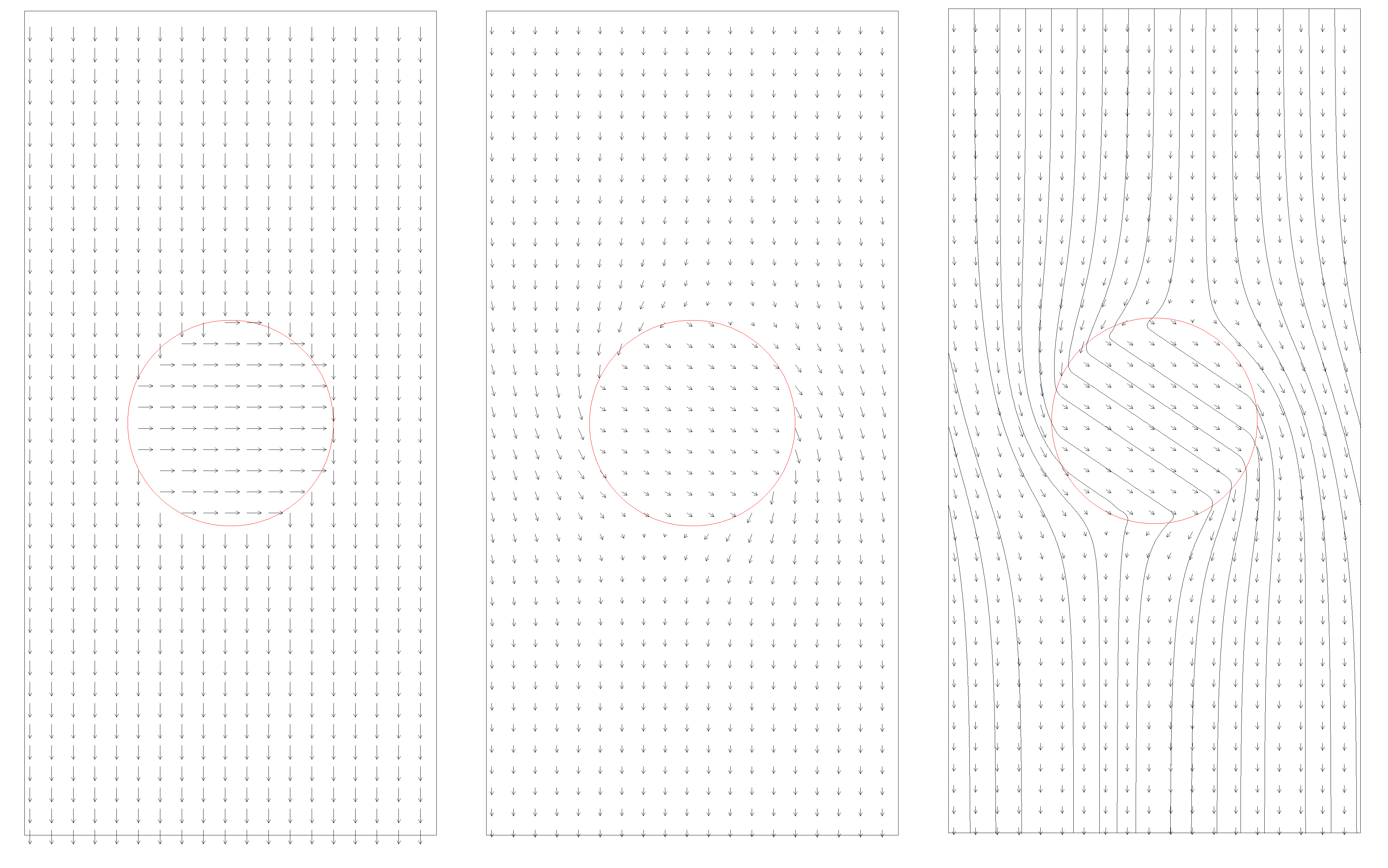
Refer to caption
Figure 6.1. The velocity fields of fluid and solid before (left) and after (middle) the augmented Hodge projection, and the streamlines (right) after projection.

Figure 6.2 validates the theorem that the orthogonality condition

⟨(𝑼h,𝒗h,𝝎h),(𝑼∗−𝑼h,𝒗∗−𝒗h,𝝎∗−𝝎h)⟩Eh=0\langle(\boldsymbol{U}^{h},\boldsymbol{v}^{h},\boldsymbol{\omega}^{h}),(\boldsymbol{U}^{*}-\boldsymbol{U}^{h},\boldsymbol{v}^{*}-\boldsymbol{v}^{h},\boldsymbol{\omega}^{*}-\boldsymbol{\omega}^{h})\rangle_{E_{h}}=0

and the stability condition ∥(𝑼h,𝒗h,𝝎h)∥Eh≤∥(𝑼∗,𝒗∗,𝝎∗)∥Eh\lVert(\boldsymbol{U}^{h},\boldsymbol{v}^{h},\boldsymbol{\omega}^{h})\rVert_{E_{h}}\leq\lVert(\boldsymbol{U}^{*},\boldsymbol{v}^{*},\boldsymbol{\omega}^{*})\rVert_{E_{h}} are satisfied for all θ∈[0,2​π]\theta\in\left[0,2\pi\right]. The numerical solution (𝑼h,𝒗h,𝝎h)(\boldsymbol{U}^{h},\boldsymbol{v}^{h},\boldsymbol{\omega}^{h}) was computed in a uniform grid 40×8040\times 80.

Refer to caption
Figure 6.2. The kinetic energy before (dashed line) and after (solid line) the augmented Hodge projection, and the inner product. This figure validates ∥(𝑼h,𝒗h,𝝎h)∥Eh≤∥(𝑼∗,𝒗∗,𝝎∗)∥Eh\lVert(\boldsymbol{U}^{h},\boldsymbol{v}^{h},\boldsymbol{\omega}^{h})\rVert_{E_{h}}\leq\lVert(\boldsymbol{U}^{*},\boldsymbol{v}^{*},\boldsymbol{\omega}^{*})\rVert_{E_{h}} and ⟨(𝑼h,𝒗h,𝝎h),(𝑼∗−𝑼h,𝒗∗−𝒗h,𝝎∗−𝝎h)⟩Eh=0\langle(\boldsymbol{U}^{h},\boldsymbol{v}^{h},\boldsymbol{\omega}^{h}),(\boldsymbol{U}^{*}-\boldsymbol{U}^{h},\boldsymbol{v}^{*}-\boldsymbol{v}^{h},\boldsymbol{\omega}^{*}-\boldsymbol{\omega}^{h})\rangle_{E_{h}}=0.

6.2. Convergence in two dimensions

We showed in Theorem 5.2 that

∥(𝑼h,𝒗h,𝝎h)−(𝑼,𝒗,𝝎∥Eh=O(h),\lVert(\boldsymbol{U}^{h},\boldsymbol{v}^{h},\boldsymbol{\omega}^{h})-(\boldsymbol{U},\boldsymbol{v},\boldsymbol{\omega}\rVert_{E_{h}}=O(h),

which implies that each of the approximations 𝑼h≃𝑼\boldsymbol{U}^{h}\simeq\boldsymbol{U}, 𝒗h≃𝒗\boldsymbol{v}^{h}\simeq\boldsymbol{v}, and 𝝎h≃𝝎\boldsymbol{\omega}^{h}\simeq\boldsymbol{\omega} is at least first-order accurate. In this example, we numerically validate the convergence order. Inside [−π2,π2]2\left[-\frac{\pi}{2},\frac{\pi}{2}\right]^{2}, a solid with mass m=1m=1 and inertia 𝕀=𝔼\mathbb{I}=\mathbb{E} is located in a domain {(x,y)|cos⁡x​cos⁡y<32}\left\{\left(x,y\right)|\cos x\cos y<\frac{\sqrt{3}}{2}\right\}. Fluid with density ρ=1\rho=1 fills the rectangle outside the solid. In this setting, the augmented Hodge projection is performed on 𝑼∗=𝑼+1ρ∇p\boldsymbol{U}^{*}=\boldsymbol{U}+\frac{1}{\rho}\nabla p, 𝒗∗=0−1m​∫Γp​𝒏​𝑑s\boldsymbol{v}^{*}=0-\frac{1}{m}\intop_{\Gamma}p\boldsymbol{n}ds, and 𝝎∗=0−𝕀−1​∫Γp​𝑱​𝑑s\boldsymbol{\omega}^{*}=0-\mathbb{I}^{-1}\intop_{\Gamma}p\boldsymbol{J}ds with 𝑼⁡(x,y)=(cos⁡x​sin⁡y,−sin⁡x​cos⁡y)\boldsymbol{U}\left(x,y\right)=\left(\cos x\sin y,-\sin x\cos y\right) and p⁡(x,y)=e−(x−1)2+yp\left(x,y\right)=e^{-\left(x-1\right)^{2}+y}.

Note that 𝑼\boldsymbol{U} satisfies the incompressibility condition ∇⋅𝑼=0\nabla\cdot\boldsymbol{U}=0 and the non-penetration condition 𝑼⋅𝒏=0\boldsymbol{U}\cdot\boldsymbol{n}=0 on the rectangular boundary as well as on the interface Γ={(x,y)|cos⁡x​cos⁡y=32}.\Gamma=\{(x,y)|\cos x\cos y=\frac{\sqrt{3}}{2}\}. Numerically computed solutions (𝑼h,𝒗h,𝝎h)(\boldsymbol{U}^{h},\boldsymbol{v}^{h},\boldsymbol{\omega}^{h}) are compared to the exact solution (𝑼,𝒗=0,𝝎=0).\left(\boldsymbol{U},\boldsymbol{v}=0,\boldsymbol{\omega}=0\right). The exact values of the boundary integrals are

∫Γp𝒏dS=[−0.61757657740494⋯,−0.35222653922478⋯]\int_{\Gamma}p\boldsymbol{n}\,dS=[-0.61757657740494\cdots,-0.35222653922478\cdots]

and

∫Γp𝑱dS=−0.0000757711760965⋯.\int_{\Gamma}p\boldsymbol{J}\,dS=-0.0000757711760965\cdots.

Table 1 reports the numerical results. The convergence order of ∥(𝑼h,𝒗h,𝝎h)−(𝑼,𝒗,𝝎)∥Eh\lVert(\boldsymbol{U}^{h},\boldsymbol{v}^{h},\boldsymbol{\omega}^{h})-(\boldsymbol{U},\boldsymbol{v},\boldsymbol{\omega})\rVert_{E_{h}} with respect to hh fluctuates, but its least squares fit, as plotted in Figure 6.3, indicates that the convergence order is 1.61.1.61. In the following estimate obtained from combining Lemma 5.1 (iii) and the last inequality in the proof of Theorem 5.2,

∥(𝑼−𝑼h,𝒗−𝒗h,𝝎−𝝎h)∥Eh≤|Γ|​((diam⁡Γ)+1)​∥∇p∥L∞2​h+O⁡(h1.5),\lVert(\boldsymbol{U}-\boldsymbol{U}^{h},\boldsymbol{v}-\boldsymbol{v}^{h},\boldsymbol{\omega}-\boldsymbol{\omega}^{h})\rVert_{E_{h}}\leq\frac{\lvert\Gamma\rvert\left((\operatorname{diam}\Gamma)+1\right)\lVert\nabla p\rVert_{L^{\infty}}}{2}\,h+O(h^{1.5}),

the first term becomes dominant and forms an upper bound of the error for sufficiently small h.h. All the errors in Figure 6.3 are certainly below the upper bound, which validates the theorem. We deduced from the theorem that each of 𝑼h≃𝑼,𝒗h≃v,𝝎h≃𝝎\boldsymbol{U}^{h}\simeq\boldsymbol{U},\boldsymbol{v}^{h}\simeq v,\boldsymbol{\omega}^{h}\simeq\boldsymbol{\omega} is at least first order accurate. Table 2 confirms the deduction.

grid h ∥(𝑼−𝑼h,𝒗−𝒗h,𝝎−𝝎h)∥Eh\lVert(\boldsymbol{U}-\boldsymbol{U}^{h},\boldsymbol{v}-\boldsymbol{v}^{h},\boldsymbol{\omega}-\boldsymbol{\omega}^{h})\rVert_{E_{h}} order
20220^{2} π20\frac{\pi}{20} 3.14×10−23.14\times 10^{-2}
40240^{2} π40\frac{\pi}{40} 5.01×10−35.01\times 10^{-3} 2.65
80280^{2} π80\frac{\pi}{80} 3.42×10−33.42\times 10^{-3} 0.551
1602160^{2} π160\frac{\pi}{160} 5.70×10−45.70\times 10^{-4} 2.58
3202320^{2} π320\frac{\pi}{320} 4.17×10−44.17\times 10^{-4} 0.451
6402640^{2} π640\frac{\pi}{640} 6.99×10−56.99\times 10^{-5} 2.57
Table 1. Convergence order in the example of two dimensions. The order fluctuates, and its least squares fitting is tried in Figure 6.3.
Refer to caption
Figure 6.3. Log-plot of the least squares fit of the errors ‖(𝑼h,𝒗h,𝝎h)−(𝑼,𝒗,𝝎)‖Eh\|\left(\boldsymbol{U}^{h},\boldsymbol{v}^{h},\boldsymbol{\omega}^{h}\right)-\left(\boldsymbol{U},\boldsymbol{v},\boldsymbol{\omega}\right)\|_{E_{h}} in the example of two dimensions. The errors are certainly below the upper bound O⁡(h).O(h).
Individual error order
∥𝑼−𝑼h∥L2\lVert\boldsymbol{U}-\boldsymbol{U}^{h}\rVert_{L^{2}} O⁡(h1.61)O(h^{1.61})
|𝒗−𝒗h|\lvert\boldsymbol{v}-\boldsymbol{v}^{h}\rvert O⁡(h1.73)O(h^{1.73})
|𝝎−𝝎h|\lvert\boldsymbol{\omega}-\boldsymbol{\omega}^{h}\rvert O⁡(h2.72)O(h^{2.72})
Table 2. The convergence order of each individual error in the sum ‖(𝑼h,𝒗h,𝝎h)−(𝑼,𝒗,𝝎)‖Eh2=ρ2​‖𝑼h−𝑼‖L22+m2​‖𝒗h−𝒗‖2+𝕀2​‖𝝎h−𝝎‖2.\|\left(\boldsymbol{U}^{h},\boldsymbol{v}^{h},\boldsymbol{\omega}^{h}\right)-\left(\boldsymbol{U},\boldsymbol{v},\boldsymbol{\omega}\right)\|_{E_{h}}^{2}=\frac{\rho}{2}\|\boldsymbol{U}^{h}-\boldsymbol{U}\|_{L^{2}}^{2}+\frac{m}{2}\|\boldsymbol{v}^{h}-\boldsymbol{v}\|^{2}+\frac{\mathbb{I}}{2}\|\boldsymbol{\omega}^{h}-\boldsymbol{\omega}\|^{2}. For the same data in Figure 6.3, the order was obtained from the least squares fit of each error.

6.3. Convergence in three dimensions

We measure the convergence order of the discrete Hodge projection in a three-dimensional example. In [−2,2]2×[−4,4][-2,2]^{2}\times[-4,4], a solid with mass m=83​πm=\frac{8}{3}\pi and inertia 𝕀=1615​π​𝔼\mathbb{I}=\frac{16}{15}\pi\,\mathbb{E} is located in a ball centered at (0,0,0)(0,0,0) of radius one. We recall that 𝔼\mathbb{E} is the 3×33\times 3 identity matrix. Fluid with density ρ=1\rho=1 fills the box outside the solid. In this setting, the augmented Hodge projection is performed on 𝑼∗=(0,0,−1)\boldsymbol{U}^{*}=(0,0,-1), 𝒗∗=(0,0,−1)\boldsymbol{v}^{*}=(0,0,-1), and 𝝎∗=(0,0,0)\boldsymbol{\omega}^{*}=(0,0,0). The non-penetration condition is imposed on the rectangular boundary. Figure 6.4 illustrates the setting.

Refer to caption
Refer to caption
Figure 6.4. The physical setting for the example of three dimensions (left) and the streamlines after the projection in section x=0{x=0} (right).

Since the exact solution is unknown, we instead measure the convergence order through ∥(𝑼2​h−𝑼h,𝒗2​h−𝒗h,𝝎2​h−𝝎h)∥Eh\lVert(\boldsymbol{U}^{2h}-\boldsymbol{U}^{h},\boldsymbol{v}^{2h}-\boldsymbol{v}^{h},\boldsymbol{\omega}^{2h}-\boldsymbol{\omega}^{h})\rVert_{E_{h}}, based on the fact that we have

∥(𝑼2​h−𝑼h,𝒗2​h−𝒗h,𝝎2​h−𝝎h)∥Eh\displaystyle\lVert(\boldsymbol{U}^{2h}-\boldsymbol{U}^{h},\boldsymbol{v}^{2h}-\boldsymbol{v}^{h},\boldsymbol{\omega}^{2h}-\boldsymbol{\omega}^{h})\rVert_{E_{h}} ≤∥(𝑼−𝑼2​h,𝒗−𝒗2​h,𝝎−𝝎2​h)∥Eh\displaystyle\leq\lVert(\boldsymbol{U}-\boldsymbol{U}^{2h},\boldsymbol{v}-\boldsymbol{v}^{2h},\boldsymbol{\omega}-\boldsymbol{\omega}^{2h})\rVert_{E_{h}}
+∥(𝑼−𝑼h,𝒗−𝒗h,𝝎−𝝎h)∥Eh\displaystyle\qquad+\lVert(\boldsymbol{U}-\boldsymbol{U}^{h},\boldsymbol{v}-\boldsymbol{v}^{h},\boldsymbol{\omega}-\boldsymbol{\omega}^{h})\rVert_{E_{h}}
=O⁡(hα+2α​hα)=O⁡(hα),\displaystyle=O(h^{\alpha}+2^{\alpha}h^{\alpha})=O(h^{\alpha}),

whenever ∥(𝑼−𝑼h,𝒗−𝒗h,𝝎−𝝎h)∥Eh=O⁡(hα)\lVert(\boldsymbol{U}-\boldsymbol{U}^{h},\boldsymbol{v}-\boldsymbol{v}^{h},\boldsymbol{\omega}-\boldsymbol{\omega}^{h})\rVert_{E_{h}}=O(h^{\alpha}) for the exact solution (𝑼,𝒗,𝝎)\left(\boldsymbol{U},\boldsymbol{v},\boldsymbol{\omega}\right).

grid hh ∥(𝑼2​h,𝒗2​h,𝝎2​h)−(𝑼h,𝒗h,𝝎h)∥Eh\lVert(\boldsymbol{U}^{2h},\boldsymbol{v}^{2h},\boldsymbol{\omega}^{2h})-(\boldsymbol{U}^{h},\boldsymbol{v}^{h},\boldsymbol{\omega}^{h})\rVert_{E_{h}} order
162×3216^{2}\times 32 14\frac{1}{4} 6.16×10−26.16\times 10^{-2}
322×6432^{2}\times 64 18\frac{1}{8} 1.62×10−21.62\times 10^{-2} 1.92
642×12864^{2}\times 128 116\frac{1}{16} 4.31×10−34.31\times 10^{-3} 1.91
1282×256128^{2}\times 256 132\frac{1}{32} 1.26×10−31.26\times 10^{-3} 1.77
2562×512256^{2}\times 512 164\frac{1}{64} 3.74×10−43.74\times 10^{-4} 1.75
Table 3. The convergence error in the example of three dimensions

Table 3 reports the numerical results, which validates the convergence order O⁡(h)O\left(h\right) shown in Theorem 5.2. Also the table shows that the order is actually far greater than one. Table 4 indicates that ∥𝑼2​h−𝑼h∥L2=O⁡(h1.6)\lVert\boldsymbol{U}^{2h}-\boldsymbol{U}^{h}\rVert_{L^{2}}=O(h^{1.6}) and |𝒗h−𝒗2​h|+|𝝎h−𝝎2​h|=O⁡(h2)\lvert\boldsymbol{v}^{h}-\boldsymbol{v}^{2h}\rvert+\lvert\boldsymbol{\omega}^{h}-\boldsymbol{\omega}^{2h}\rvert=O(h^{2}). The convergence error ∥(𝑼2​h,𝒗2​h,𝝎2​h)−(𝑼h,𝒗h,𝝎h)∥Eh\lVert(\boldsymbol{U}^{2h},\boldsymbol{v}^{2h},\boldsymbol{\omega}^{2h})-(\boldsymbol{U}^{h},\boldsymbol{v}^{h},\boldsymbol{\omega}^{h})\rVert_{E_{h}} can be regarded as a sum of ∥𝑼2​h−𝑼h∥L2\lVert\boldsymbol{U}^{2h}-\boldsymbol{U}^{h}\rVert_{L^{2}} and |𝒗h−𝒗2​h|+|𝝎h−𝝎2​h|\lvert\boldsymbol{v}^{h}-\boldsymbol{v}^{2h}\rvert+\lvert\boldsymbol{\omega}^{h}-\boldsymbol{\omega}^{2h}\rvert, when the order calculation is a matter of interests. It implies that ∥(𝑼2​h,𝒗2​h,𝝎2​h)−(𝑼h,𝒗h,𝝎h)∥Eh\lVert(\boldsymbol{U}^{2h},\boldsymbol{v}^{2h},\boldsymbol{\omega}^{2h})-(\boldsymbol{U}^{h},\boldsymbol{v}^{h},\boldsymbol{\omega}^{h})\rVert_{E_{h}} is mainly influenced by ∥𝑼2​h−𝑼h∥L2=O⁡(h1.6)\lVert\boldsymbol{U}^{2h}-\boldsymbol{U}^{h}\rVert_{L^{2}}=O(h^{1.6}) rather than by the other term, when hh becomes smaller. This explains why the convergence order in Table 3 slowly decreases toward 1.61.6.

grid hh ∥𝑼2​h−𝑼h∥L2\lVert\boldsymbol{U}^{2h}-\boldsymbol{U}^{h}\rVert_{L^{2}} order |𝒗h−𝒗2​h|+|𝝎h−𝝎2​h|\lvert\boldsymbol{v}^{h}-\boldsymbol{v}^{2h}\rvert+\lvert\boldsymbol{\omega}^{h}-\boldsymbol{\omega}^{2h}\rvert order
162×3216^{2}\times 32 14\frac{1}{4} 2.65×10−22.65\times 10^{-2} 5.56×10−25.56\times 10^{-2}
322×6432^{2}\times 64 18\frac{1}{8} 8.74×10−38.74\times 10^{-3} 1.60 1.36×10−21.36\times 10^{-2} 2.03
642×12864^{2}\times 128 116\frac{1}{16} 2.61×10−32.61\times 10^{-3} 1.74 3.43×10−33.43\times 10^{-3} 1.98
1282×256128^{2}\times 256 132\frac{1}{32} 9.30×10−49.30\times 10^{-4} 1.48 8.62×10−48.62\times 10^{-4} 1.99
2562×512256^{2}\times 512 164\frac{1}{64} 3.50×10−43.50\times 10^{-4} 1.60 2.16×10−42.16\times 10^{-4} 2.00
Table 4. The convergence errors of ∥𝑼2​h−𝑼h∥L2\lVert\boldsymbol{U}^{2h}-\boldsymbol{U}^{h}\rVert_{L^{2}} and |𝒗h−𝒗2​h|+|𝝎h−𝝎2​h|\lvert\boldsymbol{v}^{h}-\boldsymbol{v}^{2h}\rvert+\lvert\boldsymbol{\omega}^{h}-\boldsymbol{\omega}^{2h}\rvert in the example of three dimensions

7. Conclusion and comment

In this work, we have studied a Fluid-Solid interaction by taking a monolithic treatment on fluid-solid interaction. It is based on the fact that fluid velocity field 𝑼\boldsymbol{U} and solid velocities 𝒗\boldsymbol{v} and 𝝎\boldsymbol{\omega} do not separately proceed but as a whole by a combined state variable (𝑼,𝒗,𝝎)(\boldsymbol{U},\boldsymbol{v},\boldsymbol{\omega}). We introduced the so-called augmented Hodge decomposition of the state variable into two orthogonal components, which is a variation of the Hodge decomposition. The decomposition enables us to decouple the computations of the velocity and the pressure in the incompressible Navier-Stokes equation. Then, the decomposition is fulfilled by solving an elliptic equation for the pressure with non-local Robin type boundary condition. We have shown the existence, uniqueness and the regularity of the solution to the equation. The monolithic treatment leads to the stability that the kinetic energy does not increase in the projection step. Using an Heaviside function, we expressed the boundary condition independent of the interface. We proposed a numerical method producing the numerical solution at least with first order accuracy. Also, we showed that the unique decomposition and orthogonality also hold in the discrete setting. We carried out numerical experiments for 2 and 3 dimensions and the numerical tests validate our analysis and arguments. Even though the experiments supports our arguments, ∥(𝑼h,𝒗h,𝝎h)−(𝑼,𝒗,𝝎)∥Eh=O⁡(h),\lVert(\boldsymbol{U}^{h},\boldsymbol{v}^{h},\boldsymbol{\omega}^{h})-(\boldsymbol{U},\boldsymbol{v},\boldsymbol{\omega})\rVert_{E_{h}}=O(h), it reveals that the convergence order is greater than one and the error is mainly influenced by ∥𝑼2​h−𝑼h∥L2=O⁡(h1.6)\lVert\boldsymbol{U}^{2h}-\boldsymbol{U}^{h}\rVert_{L^{2}}=O(h^{1.6}) rather than by the other term, when hh becomes smaller. The analysis for the phenomenon would involve very different arguments from the current one, and we put it off to future work.

References

  • [1] S. Badia, F. Nobile, and C. Vergara, Robin-Robin preconditioned Krylov methods for fluid-structure interaction problems, Comput. Methods Appl. Mech. Eng., 198, 2768–2784, 2009.
  • [2] S. Badia, A. Quaini, and A. Quarteroni, Modular vs. non-modular preconditioners for fluid?structure systems with large addedmass effect, Comput. Methods Appl. Mech. Eng., 197, 4216–4232, 2008.
  • [3] C. Batty, F. Bertails, and R. Bridson, A fast variational framework for accurate solid-fluid coupling, ACM Trans. Graph. (SIGGRAPH Proc.), 26(3), 2007.
  • [4] J. B. Bell, P. Colella, and H. M. Glaz, A second order projection method for the incompressible Navier-Stokes equations, J. Comput. Phys., 85, 257–283, 1989.
  • [5] I. Borazjani, L. Ge, and F. Sotiropoulos, Curvilinear immersed boundary method for simulating fluid structure interaction with complex 3D rigid bodies, J. Comput. Phys. 227(16), 7587–7620, 2008.
  • [6] R. Bridson, Fluid simulation for computer graphics, A K Pters, Ltd., 2008, 888 Worcester Street, Wellesley, MA 02482.
  • [7] D. Brown, R. Cortez, and M. Minion, Accurate projection methods for the incompressible Navier-Stokes equations, J. Comput. Phys., 168, 464–499, 2001.
  • [8] M. Bukač, I. Yotov, and P. Zunino, An operator splitting approach for the interaction between a fluid and a multilayered poroelastic structure, Numerical Methods for Partial Differential Equations, 31, 1054–1100, 2015.
  • [9] P. Causin, J. Gerbeau, and F. Nobile, Added-mass effect in the design of partitioned algorithms for fluid-structure problems, Comput. Methods Appl. Mech. Eng., 194, 42–44, 2005.
  • [10] S. K. Chakrabarti (Ed.), Numerical Models in Fluid Structure Interaction, Advances in Fluid Mechanics, 42, WIT Press, 2005.
  • [11] Z. Q. Chen, R. J. Williams, and Z. Zhao, A Sobolev inequality and Neumann heat kernel estimate for unbounded domains, Math. Res. Lett., 1, 177–184, 1994.
  • [12] A. Chorin, A numerical method for solving incompressible viscous flow problems, J. Comput. Phys., 2, 12–26, 1967.
  • [13] J. Degroote, P. Bruggeman, R. Haelterman, and J. Vierendeels, Stability of a coupling technique for partitioned solvers in FSI applications, Comput. Struct., 86, 2224–2234, 2008.
  • [14] E. H. Dowell and K. C. Hall, Modeling of fluid-structure interaction, Annual Review of Fluid Mechanics, 33, 445–490, 2001.
  • [15] L. C. Evans, Partial differential equations, Graduate Studies in Mathematics, vol., 19, Amer. Math. Soc., 1998.
  • [16] C. Farhat, K. van der Zee,and P. Geuzaine, Provably second-order time-accurate loosely-coupled solution algorithms for transient nonlinear computational aeroelasticity, Comput. Methods Appl. Mech. Eng., 195, 1973–2001, 2006.
  • [17] M. Fernández, Incremental displacement-correction schemes for incompressible fluid-structure interaction, Numerische Mathematik, 123, 21–65, 2013
  • [18] M. Fernández and J. Mullaert, Convergence and error analysis for a class of splitting schemes in incompressible fluid-structure interaction, IMA Journal of Numerical Analysis, (2015), p. drv055.
  • [19] C. Förster, W. A. Wall, and E. Ramm, Artificial added mass instabilities in sequential staggered coupling of nonlinear structures and incompressible viscous flows, Comput. Methods Appl. Mech. Eng., 196(7), 1278–1293, 2007.
  • [20] M. Gee, U. Küttler, and W. Wall, Truly monolithic algebraic multigrid for fluid-structure interaction, Int. J. Numer. Meth. Eng., 85, 987–1016, 2011.
  • [21] F. Gibou, R. Fedkiw, L.-T. Cheng, and M. Kang, A second-order-accurate symmetric discretization of the Poisson equation on irregular domains, J. Comput. Phys., 176, 205–227, 2002.
  • [22] F. Gibou and C. Min, Efficient symmetric positive definite second-order accurate monolithic solver for fluid/solid interactions, J. Comput. Phys., 231, 3245–3263, 2012.
  • [23] D. Gilbarg and N. S. Trudinger, Elliptic partial differential equations of second order, Reprint of the 1998 ed. Springer-Verlag, Berlin, 2001.
  • [24] J. T. Grétarsson, N. Kwatra, and R. Fedkiw, Numerically stable fluid-structure interactions between compressible flow and solid structures, J. Comput. Phys., 230, 3062–3084, 2011.
  • [25] J. L. Guermond, P. Minev, and J. Shen, An overview of projection methods for incompressible flows, Comput. Methods Appl. Mech. Engrg., 195, 6011?6045, 2006
  • [26] F. Harlow and J. Welch, Numerical calculation of time-dependent viscous incompressible flow of fluids with free surfaces, Physics of Fluids, 8, 2182–2189, 1965.
  • [27] M. Heil, A. Hazel, and J. Boyle, Solvers for large-displacement fluid-structure interaction problems: segregated versus monolithic approaches, Comput. Mech., 43, 91–101, 2008.
  • [28] H. Helmholtz, On integrals of the hydrodynamic equations which correspond to vortex motions, Journal fur die reine und angewandte Mathematik, 55, 25–55, 1858.
  • [29] B. Hübner, E. Walhorn, and D. Dinkler, A monolithic approach to fluid-structure interaction using space-time finite elements, Comput. Methods Appl. Mech. Eng., 193, 2087–2104, 2004.
  • [30] J. Kim and P. Moin, Application of a fractional-step method to incompressible Navier-Stokes equations, J. Comput. Phys., 59, 308–323, 1985.
  • [31] E. W. Liu and J. G. Liu, Gauge method for viscous incompressible flows, Comm. Math. Sci., 1, 317–332, 2003.
  • [32] C. Michler, S. J. Hulshoff, E. H. van Brummelen, and R. de Borst, A monolithic approach to fluid-structure interaction, Comput. Fluids, 33, 839–848, 2004
  • [33] C. Min and G. Yoon, Convergence analysis on Gibou-Min method for the scalar field in Hodge-Helmholtz decomposition, J. Korean Soc. Ind. Appl. Math., 18, 305–316, 2014.
  • [34] H. J.-P. Morand and R. Ohayon, Fluid-Structure Interaction: Applied Numerical Methods, Wiley, 1995.
  • [35] B. Muha and S. Čanić, Existence of a Weak Solution to a Nonlinear Fluid-Structure Interaction Problem Modeling the Flow of an Incompressible, Viscous Fluid in a Cylinder with Deformable Walls, Arch. Rational Mech. Anal., 207, 919–968, 2013.
  • [36] Y. T. Ng, C. Min, and F. Gibou, An efficient fluid-solid coupling algorithm for single-phase flows, J. Comput. Phys., 228, 8807–8829, 2009.
  • [37] F. Nobile and C. Vergara, An effective fluid-structure interaction formulation for vascular dynamics by generalized Robin conditions, SIAM J. Sci. Comput., 30, 731–763, 2008.
  • [38] C. Pozrikidis, Introduction to theoretical and computational fluid dynamics, Oxford university press, 1997.
  • [39] J. W. Purvis and J. E. Burkhalter, Prediction of critical Mach number for store configurations, AIAA J., 17, 1170–1177, 1979.
  • [40] P. B. Ryzhakov, R. Rossi, S. R. Idelsohn, and E. Oñate, A monolithic Lagrangian approach for fluid-structure interaction problems, Comput. Mech., 46, 883–899, 2010.
  • [41] M. Uhlmann, An immersed boundary method with direct forcing for the simulation of particulate flows, J. Comput. Phys., 209(2), 448–476, 2005.
  • [42] E. Walhorn, A. Kölke, B. Hübner, and D. Dinkler, Fluid-structure coupling within a monolithic model involving free surface flows, Comput. Struct., 83, 2100–2111, 2005.
  • [43] D. Xiu and G. Karniadakis, A semi-Lagrangian high-order method for Navier-Stokes equations, J. Comput. Phys., 172, 658–684, 2001.
  • [44] G. Yoon and C. Min, Analyses on the finite difference method by Gibou et al. for Poisson equation, J. Comput. Phys., 280, 184–194, 2015.
  • [45] G. Yoon and C. Min, Convergence analysis of the standard central finite difference method for Poisson equation, J. Sci. Comput., accepted.
  • [46] G. Yoon, J.-H. Park, and C. Min, Convergence analysis on the Gibou-Min method for the Hodge projection, Commun. Math. Sci., submitted.