跳到论文正文
W Papers独立论文阅读器 arXiv:1610.03140 论文正文 计算阅读时间 · 0%
引用这篇论文根据当前论文元数据生成,正式投稿前建议核对。


License: arXiv.org perpetual non-exclusive license
arXiv:1610.03140v2 [math.DS] 05 May 2017

On the Global Dynamics of an Electroencephalographic Mean Field Model of the Neocortex

Farshad Shirani ††thanks: School of Aerospace Engineering, Georgia Institute of Technology, Atlanta, GA 30332    Wassim M. Haddad ††thanks: School of Aerospace Engineering, Georgia Institute of Technology, Atlanta, GA 30332    Rafael de la Llave ††thanks: School of Mathematics, Georgia Institute of Technology, Atlanta, GA 30332
Abstract

This paper investigates the global dynamics of a mean field model of the electroencephalogram developed by Liley et al., 2002. The model is presented as a system of coupled ordinary and partial differential equations with periodic boundary conditions. Existence, uniqueness, and regularity of weak and strong solutions of the model are established in appropriate function spaces, and the associated initial-boundary value problems are proved to be well-posed. Sufficient conditions are developed for the phase spaces of the model to ensure nonnegativity of certain quantities in the model, as required by their biophysical interpretation. It is shown that the semigroups of weak and strong solution operators possess bounded absorbing sets for the entire range of biophysical values of the parameters of the model. Challenges towards establishing a global attractor for the model are discussed and it is shown that there exist parameter values for which the constructed semidynamical systems do not possess a compact global attractor due to the lack of the asymptotic compactness property. Finally, using the theoretical results of the paper, instructive insights are provided into the complexity of the behavior of the model and computational analysis of the model.

1 Introduction

Inspired by the seminal work of Alan Hodgkin and Andrew Huxley on modeling the flow of ionic currents through the membrane of a giant nerve fiber, numerous biophysical and mathematical models have been developed towards understanding the neurophysiology of the central nervous system and the underlying mechanism of the various phenomena that emerge during its vital operation in the body; many of which still remain a mystery to researchers [26, 17, 42, 54]. In particular, exploring the core component of the central nervous system—the brain—substantial effort has been devoted to develop models at different levels of scope; from the molecular and intercellular level dealing with the transportation of ions and the enzymatic kinetics of neurotransmitter-receptor binding at ion channels; to the single cell and intracellular level dealing with the creation and transmission of action potential; to the population and neuronal network level dealing with the average behavior and synchronized activity of neuronal ensembles; to the system level dealing with the systematic operation and interaction between cortical and subcortical components of the brain; and eventually, to the behavioral and cognitive level dealing with the integrated mental activity and the creation of mind [29, 1, 15, 30, 22, 55, 46, 48].

As an effective methodology for developing models at the population and network level, mean field theory has been employed to construct approximate models for interconnected populations of neurons by averaging the effect of all other neurons on a given individual neuron inside a population. The resulting averaged neuron can be used to analyze the overall temporal behavior of a single population of neurons—leading to a neural mass model—or can be considered as a locally averaged component of a continuum of neural populations—leading to a spatio-temporal mean field model. These models are particularly useful in analyzing the electrophysiological activity of neuronal ensembles using local field potentials and electroencephalograms [43, 40, 45, 10].

The evolution equations that describe a mean field model of neural activity in the cortex are in the form of a system of partial differential equations, or a system of coupled ordinary and partial differential equations. The theory of infinite-dimensional dynamical systems is hence used to analyze the global dynamics and long-term behavior of these systems. The classical approach to this problem follows several steps. First, existence, uniqueness, and regularity of solutions are established for all positive time in appropriately chosen problem-dependent function spaces, and the well-posedness of the problem is confirmed. Second, a semidynamical framework is constructed over a positively invariant complete normed space—the phase space for the evolution of the solutions—and is shown to possess bounded absorbing sets. Asymptotic compactness of the semigroup of solution operators is then ensured to guarantee the existence of a global attractor, which is a compact strictly invariant attracting set and contains all the information regarding the asymptotic behavior of the model. Third, the Hausdorff or fractal dimension of the global attractor is estimated to show that the attractor is finite dimensional, so that the asymptotic dynamics of the system is determined by a finite number of degrees of freedom. Fourth, the existence of an inertial manifold is established, which is a smooth finite-dimensional invariant manifold containing the global attractor. Consequently, the dynamics on the attractor can be presented by a finite set of ordinary differential equations and further characterized to give the overall picture of the long-term behavior of the system [24, 51, 7, 44, 25].

In this paper, we investigate the mean field model proposed in [36] for understanding the electrical activity in the neocortex as observed in the electroencephalogram (EEG). This model, which is comprised of a system of coupled ordinary and partial differential equations in a two-dimensional space, has been widely used in the literature to study the alpha- and gamma-band rhythmic activity in the cortex [5, 4], phase transition and burst suppression in cortical neurons during general anesthesia [37, 6, 49], the effect of anesthetic drugs on the EEG [2, 19], and epileptic seizures [35, 33, 31, 32]. Open-source tools for numerical implementation of the model and computation of equilibria and time-periodic solutions are developed in [23]. Complexity of the dynamics of the model, including periodic and pseudo-periodic solutions, chaotic behavior, multistability, and bifurcation are studied in [20, 21, 13, 11, 12, 52, 53].

The above results, however, are mainly computational or use approximate versions of the model. A rigorous analysis of the dynamics of the model in an infinite-dimensional dynamical system framework as outlined above is not available in the literature. In particular, the basic problems of well-posedness of the initial-boundary value problem associated with the model and regularity of the solutions remain uninvestigated. It is not known under what conditions, if any, the components of the solutions of the model that are associated with nonnegative biophysical quantities remain nonnegative for all time. The solutions that take negative values for such quantities—even for a small interval of time in distant future—cannot represent a biophysically plausible dynamics of the electrical activity in the neocortex.

The aim of this paper is to study the global dynamics of the mean field model discussed above, to ensure its biophysical plausibility, and to provide the basic analytical results required for characterization of the long-term dynamics of the model. Specifically, we follow the first two steps of the classical analysis approach to investigate the problem of existence or nonexistence of a global attractor.

This paper is organized as follows. In Section 2, we introduce notation and recall key definitions that are necessary for developing the results in this paper. In Section 3, we give a description of the anatomical structure of the neocortex and the physiological interactions that underly the construction of the model. Moreover, we present the mathematical structure of the model as a system of coupled ordinary-partial differential equations with initial values and periodic boundary conditions. In Section 4, following the first step of the classical analysis approach, we prove the existence and uniqueness of weak and strong solutions for the proposed initial value problem and analyze the regularity of these solutions.

As in the second step of the classical analysis approach, in Section 5 we define semigroups of weak and strong solution operators and show their continuity properties. Moreover, we establish sufficient conditions on the phase spaces that ensure biophysical plausibility of the evolution of the solutions under the associated semidynamical systems. In Section 6, we show that the semigroups of solution operators possess bounded absorbing sets for all possible values of the biophysical parameters of the model. In Section 7, we discuss challenges towards establishing a global attractor for the model, and in particular, we show that there exist sets of values for the biophysical parameters of the model such that the associated semigroups of solution operators do not possess a compact global attractor. We conclude the paper in Section 8 with a discussion on the results developed in the paper and their application to computational analysis of the model.

2 Notation and Preliminaries

The notation used in this paper is fairly standard. Specifically, ℝn\mathbb{R}^{n} denotes the nn-dimensional real Euclidean space and ℝm×n\mathbb{R}^{m\times n} denotes the space of real m×nm\times n matrices. A point x∈ℝnx\in\mathbb{R}^{n} is presented by the nn-tuple x=(x1,…,xn)x=(x_{1},\dots,x_{n}) or, when it appears in matrix operations, by the column vector x=[x1⋯xn]Tx=\left[\begin{array}[]{ccc}x_{1}&\cdots&x_{n}\end{array}\right]^{\mathrm{T}}, where (⋅)T(\cdot)^{\mathrm{T}} denotes transpose. The nonnegative cone {x∈ℝn:xj≥0 for j=1,…,n}\{x\in\mathbb{R}^{n}:x_{j}\geq 0\text{ for }j=1,\dots,n\} is denoted by ℝ+n\mathbb{R}_{+}^{n}. A sequence of points in ℝn\mathbb{R}^{n} is denoted by {x(l)}l=1∞\big\{x^{(l)}\big\}_{l=1}^{\infty}, with the jjth component of x(l)x^{(l)} denoted by xj(l)x_{j}^{(l)}. Moreover, the trace of a square matrix A∈ℝn×nA\in\mathbb{R}^{n\times n} is denoted by tr⁡A\trace A and a block-diagonal matrix DD with kk blocks D1,…,DkD_{1},\dots,D_{k} is denoted by diag⁡(D1,…,Dk)\diag(D_{1},\dots,D_{k}). For x,y∈ℝnx,y\in\mathbb{R}^{n}, we write x≥yx\geq y to denote component-wise inequality, that is, xj≥yjx_{j}\geq y_{j}, j=1,…,nj=1,\dots,n. For A,B∈ℝn×nA,B\in\mathbb{R}^{n\times n} we write A≥BA\geq B to denote A−BA-B is positive semidefinite. Finally, we denote by 0n×n0_{n\times n} and In×nI_{n\times n} the zero and identity matrices in ℝn×n\mathbb{R}^{n\times n}, respectively. We write II for the identity operator in other vector spaces.

For an inner product space 𝒰\mathcal{U}, we denote the associated inner product by (⋅,⋅)𝒰\big(\cdot,\cdot\big)\hskip-0.85358pt_{\mathcal{U}} and the norm generated by the inner product by ∥⋅∥𝒰\big\|\cdot\big\|_{\mathcal{U}}. For a Hilbert space 𝒰\mathcal{U}, we denote the pairing of 𝒰\mathcal{U} with its dual space 𝒰∗\mathcal{U}^{\ast} by ⟨⋅,⋅⟩𝒰\big\langle\cdot,\cdot\big\rangle\hskip-0.85358pt_{\mathcal{U}}. In particular, for 𝒰=ℝn\mathcal{U}=\mathbb{R}^{n} we write (⋅,⋅)ℝn\big(\cdot,\cdot\big)\hskip-0.85358pt_{\mathbb{R}^{n}} and ∥⋅∥ℝn\big\|\cdot\big\|_{\mathbb{R}^{n}} for the standard inner product and the Euclidean norm, respectively. Similarly, for 𝒰=ℝm×n\mathcal{U}=\mathbb{R}^{m\times n} we write (⋅,⋅)ℝm×n\big(\cdot,\cdot\big)\hskip-0.85358pt_{\mathbb{R}^{m\times n}} for the standard inner product and ∥⋅∥ℝm×n\big\|\cdot\big\|_{\mathbb{R}^{m\times n}} for the associated inner product norm. Moreover, we denote the vector 1-, 2-, and ∞\infty-norms in ℝn\mathbb{R}^{n} by ∥⋅∥1\big\|\cdot\big\|_{1}, ∥⋅∥2=∥⋅∥ℝn\big\|\cdot\big\|_{2}=\big\|\cdot\big\|_{\mathbb{R}^{n}}, and ∥⋅∥∞\big\|\cdot\big\|_{\infty}, respectively. The matrix 1-, 2-, and ∞\infty-norms in ℝm×n\mathbb{R}^{m\times n} induced, respectively, by the vector 1-, 2-, and ∞\infty-norms in ℝn\mathbb{R}^{n} are denoted by ∥⋅∥1\big\|\cdot\big\|_{1}, ∥⋅∥2\big\|\cdot\big\|_{2} and ∥⋅∥∞\big\|\cdot\big\|_{\infty}.

Let Ω\Omega be an open subset of ℝn\mathbb{R}^{n} denoting the space domain of a given dynamical system, with x∈Ωx\in\Omega denoting a spatial point in Ω\Omega. The time domain of the system is given by the closed interval [0,T]⊂ℝ[0,T]\subset\mathbb{R}, T>0T>0, with the temporal point tt. For a function u:[0,T]→ℝu:[0,T]\rightarrow\mathbb{R}, the kkth-order total derivative with respect to tt at t0t_{0} is denoted by dtk​u​(t0)\mathrm{d}_{t}^{k}u(t_{0}). For k=1k=1, we write dt​u​(t0)\mathrm{d}_{t}u(t_{0}). For a function u⁡(x,t):Ω×[0,T]→ℝu(x,t):\Omega\times[0,T]\rightarrow\mathbb{R}, the kkth-order partial derivative with respect to tt at (x0,t0)(x_{0},t_{0}) is denoted by ∂tku⁡(x0,t0)\partial_{t}^{k}u(x_{0},t_{0}) and the kkth-order partial derivative with respect to xjx_{j} at (x0,t0)(x_{0},t_{0}) is denoted by ∂xjku⁡(x0,t0)\partial_{x_{j}}^{k}u(x_{0},t_{0}), j=1,…,nj=1,\dots,n. For k=1k=1, we write ∂tu⁡(x0,t0)\partial_{t}u(x_{0},t_{0}) and ∂xju⁡(x0,t0)\partial_{x_{j}}u(x_{0},t_{0}). The gradient of uu in Ω\Omega is denoted by ∂xu\partial_{x}u and is given by ∂xu:=(∂x1u,…,∂xnu)\partial_{x}u:=(\partial_{x_{1}}u,\dots,\partial_{x_{n}}u). The Laplacian of uu in Ω\Omega is denoted by Δ​u\Delta u and is given by Δu:=(∂x12+⋯+∂xn2)\Delta u:=(\partial_{x_{1}}^{2}+\dots+\partial_{x_{n}}^{2}). For a vector-valued function u⁡(x,t):Ω×[0,T]→ℝmu(x,t):\Omega\times[0,T]\rightarrow\mathbb{R}^{m} we interpret u⁡(x,t)u(x,t) as the mm-tuple u⁡(x,t)=(u1​(x,t),…,um​(x,t))u(x,t)=(u_{1}(x,t),\dots,u_{m}(x,t)), where each component uj​(x,t)u_{j}(x,t), j=1,…,mj=1,\dots,m, is a scalar-valued function on Ω×[0,T]\Omega\times[0,T]. In this case, ∂xu⁡(x,t)∈ℝm×n\partial_{x}u(x,t)\in\mathbb{R}^{m\times n} is the gradient of uu and the vector Laplacian Δ​u\Delta u is given by Δ​u​(x,t):=(Δ​u1​(x,t),…,Δ​um​(x,t))∈ℝm\Delta u(x,t):=(\Delta u_{1}(x,t),\dots,\Delta u_{m}(x,t))\in\mathbb{R}^{m}, assuming Cartesian coordinates.

For every integer k≥0k\geq 0, the space of kk-times continuously differentiable real-valued functions on Ω\Omega is denoted by Ck​(Ω)C^{k}(\Omega). The space Ck​(Ω¯)C^{k}(\overline{\Omega}) consists of all functions in Ck​(Ω)C^{k}(\Omega) that, together with all of their partial derivatives up to the order kk, are uniformly continuous in bounded subsets of Ω\Omega. Moreover, for 0<λ≤10<\lambda\leq 1, the Hölder space Ck,λ​(Ω¯)C^{k,\lambda}(\overline{\Omega}) is a subspace of Ck​(Ω¯)C^{k}(\overline{\Omega}) consisting of functions whose partial derivatives of order kk are Hölder continuous with exponent λ\lambda; see [9, Sec. 1.18] for details. We use Cc∞​(Ω)C_{\mathrm{c}}^{\infty}(\Omega) to denote the space of infinitely differentiable real-valued functions with compact support in Ω\Omega. Moreover, we denote by Lloc1​(Ω)L_{\rm loc}^{1}(\Omega) the space of locally integrable real-valued functions on Ω\Omega. Then, for every function u∈Lloc1​(Ω)u\in L_{\rm loc}^{1}(\Omega) and any multi index α\alpha with |α|≥1|\alpha|\geq 1, the weak partial derivative of uu in Lloc1​(Ω)L_{\rm loc}^{1}(\Omega), of order |α||\alpha|, is defined by the distribution uαu^{\alpha} that stisfies

∫Ωuα​ϕ​𝑑x=(−1)|α|​∫Ωu​∂αϕ​𝑑xfor all ​ϕ∈Cc∞​(Ω),\int_{\Omega}u^{\alpha}\phi\,\mathrm{d}x=(-1)^{|\alpha|}\int_{\Omega}u\partial^{\alpha}\phi\,\mathrm{d}x\quad\text{for all }\phi\in C_{\mathrm{c}}^{\infty}(\Omega),

where dx=dx1⋯dxn\mathrm{d}x=\mathrm{d}x_{1}\cdots\mathrm{d}x_{n} is the Lebesgue measure on ℝn\mathbb{R}^{n}; see [9, Sec. 6.3] for details. With a minor abuse of notation, we use ∂tk\partial_{t}^{k} and ∂xk\partial_{x}^{k} to denote the kkth-order weak—as well as classical—partial derivatives with respect to tt and xx, respectively. The distinction will be clear from the context, or will otherwise be explicitly specified.

The Hilbert space of vector-valued Lebesgue measurable functions u:Ω→ℝmu:\Omega\rightarrow\mathbb{R}^{m} with finite L2L^{2}-norm is denoted by L2​(Ω,ℝm)L^{2}(\Omega;\mathbb{R}^{m}), with associated inner product and norm given by

(u,v)L2​(Ω,ℝm):=∫Ω(u⁡(x),v⁡(x))ℝm​𝑑x,‖u‖L2​(Ω,ℝm):=[∫Ω‖u⁡(x)‖ℝm2​𝑑x]12.\displaystyle\big(u,v\big)\hskip-0.85358pt_{L^{2}(\Omega;\mathbb{R}^{m})}:=\int_{\Omega}\big(u(x),v(x)\big)\hskip-0.85358pt_{\mathbb{R}^{m}}\mathrm{d}x,\quad\big\|u\big\|_{L^{2}(\Omega;\mathbb{R}^{m})}:=\left[\int_{\Omega}\big\|u(x)\big\|_{\mathbb{R}^{m}}^{2}\mathrm{d}x\right]^{\frac{1}{2}}.

The Banach space of vector-valued Lebesgue measurable functions u:Ω→ℝmu:\Omega\rightarrow\mathbb{R}^{m} with finite L∞L^{\infty}-norm is denoted by L∞​(Ω,ℝm)L^{\infty}(\Omega;\mathbb{R}^{m}), with the norm

‖u‖L∞​(Ω,ℝm):=ess​supx∈Ω⁡‖u⁡(x)‖∞.\displaystyle\big\|u\big\|_{L^{\infty}(\Omega;\mathbb{R}^{m})}:=\esssup_{x\in\Omega}\big\|u(x)\big\|_{\infty}.

The Sobolev space of vector-valued functions u∈Lp​(Ω,ℝm)u\in L^{p}(\Omega;\mathbb{R}^{m}) whose all llth-order weak derivatives ∂xlu\partial_{x}^{l}u, l≤kl\leq k, exist and belong to Lp​(Ω,ℝm×nl)L^{p}(\Omega;\mathbb{R}^{m\times n^{l}}) is denoted by Wk,p​(Ω,ℝm)W^{k,p}(\Omega;\mathbb{R}^{m}). When p=2p=2, the Sobolev spaces Wk,2​(Ω,ℝm)W^{k,2}(\Omega;\mathbb{R}^{m}) are Hilbert spaces for all k∈[0,∞)k\in[0,\infty), and are denoted by Hk​(Ω,ℝm):=Wk,2​(Ω,ℝm)H^{k}(\Omega;\mathbb{R}^{m}):=W^{k,2}(\Omega;\mathbb{R}^{m}). Specifically, H0​(Ω,ℝm)=L2​(Ω,ℝm)H^{0}(\Omega;\mathbb{R}^{m})=L^{2}(\Omega;\mathbb{R}^{m}), and H1​(Ω,ℝm)H^{1}(\Omega;\mathbb{R}^{m}) is a Hilbert space with the inner product

(u,v)H1​(Ω,ℝm)\displaystyle\big(u,v\big)\hskip-0.85358pt_{H^{1}(\Omega;\mathbb{R}^{m})} :=(u,v)L2​(Ω,ℝm)+(∂xu,∂xv)L2​(Ω,ℝm×n).\displaystyle:=\big(u,v\big)\hskip-0.85358pt_{L^{2}(\Omega;\mathbb{R}^{m})}+\big(\partial_{x}u,\partial_{x}v\big)\hskip-0.85358pt_{L^{2}(\Omega;\mathbb{R}^{m\times n})}.

Moreover, H2​(Ω,ℝm)H^{2}(\Omega;\mathbb{R}^{m}) is a Hilbert space with the inner product

(u,v)H2​(Ω,ℝm)\displaystyle\big(u,v\big)\hskip-0.85358pt_{H^{2}(\Omega;\mathbb{R}^{m})} :=(u,v)L2​(Ω,ℝm)+(∂xu,∂xv)L2​(Ω,ℝm×n)+(∂x2u,∂x2v)L2​(Ω,ℝm×n2).\displaystyle:=\big(u,v\big)\hskip-0.85358pt_{L^{2}(\Omega;\mathbb{R}^{m})}+\big(\partial_{x}u,\partial_{x}v\big)\hskip-0.85358pt_{L^{2}(\Omega;\mathbb{R}^{m\times n})}+\big(\partial_{x}^{2}u,\partial_{x}^{2}v\big)\hskip-0.85358pt_{L^{2}(\Omega;\mathbb{R}^{m\times n^{2}})}.

Let Ω=(0,ω1)×⋯×(0,ωn)\Omega=(0,\omega_{1})\times\cdots\times(0,\omega_{n}), where ωj>0\omega_{j}>0, j=1,…,nj=1,\dots,n, be an open rectangle in ℝn\mathbb{R}^{n}. A function u:ℝn→ℝu:\mathbb{R}^{n}\rightarrow\mathbb{R} is called Ω\Omega-periodic if it is periodic in each direction, that is,

u(x+ωjej)=u(x),j=1,…,n,x∈ℝn,u(x+\omega_{j}e_{j})=u(x),\quad j=1,\dots,n,\quad x\in\mathbb{R}^{n},

where eje_{j} is the unit vector in the jjth direction. Define the space Cper∞​(Ω)C_{\rm per}^{\infty}(\Omega) as the restriction to Ω\Omega of the space of infinitely differentiable Ω\Omega-periodic functions. Then, the Sobolev space Hperk​(Ω)H_{\rm per}^{k}(\Omega), k≥0k\geq 0, is defined by the completion of Cper∞​(Ω)C_{\rm per}^{\infty}(\Omega) in Hk​(Ω)H^{k}(\Omega); see [44, Definition 5.37] or, for an equivalent definition, [51, p. 50] . A vector-valued function u:ℝn→ℝmu:\mathbb{R}^{n}\rightarrow\mathbb{R}^{m} is Ω\Omega-periodic if each of its components uj:ℝn→ℝu_{j}:\mathbb{R}^{n}\rightarrow\mathbb{R}, j=1,…,mj=1,\dots,m, is Ω\Omega-periodic. The spaces Cper∞​(Ω,ℝm)C_{\rm per}^{\infty}(\Omega;\mathbb{R}^{m}) and Hperk​(Ω,ℝm)H_{\rm per}^{k}(\Omega;\mathbb{R}^{m}) are then defined accordingly. It follows from Green’s formula that

(2.1) (−Δ​u,v)Lper2​(Ω,ℝm)\displaystyle\big(-\Delta u,v\big)\hskip-0.85358pt_{L_{\rm per}^{2}(\Omega;\mathbb{R}^{m})} =(∂xu,∂xv)Lper2​(Ω,ℝm×n),\displaystyle=\big(\partial_{x}u,\partial_{x}v\big)\hskip-0.85358pt_{L_{\rm per}^{2}(\Omega;\mathbb{R}^{m\times n})},
((−Δ+I)​u,v)Lper2​(Ω,ℝm)\displaystyle\big((-\Delta+I)u,v\big)\hskip-0.85358pt_{L_{\rm per}^{2}(\Omega;\mathbb{R}^{m})} =(u,v)Hper1​(Ω,ℝm),\displaystyle=\big(u,v\big)\hskip-0.85358pt_{H_{\rm per}^{1}(\Omega;\mathbb{R}^{m})},
(−Δ​u,(−Δ+I)​u)Lper2​(Ω,ℝm)\displaystyle\big(-\Delta u,(-\Delta+I)u\big)\hskip-0.85358pt_{L_{\rm per}^{2}(\Omega;\mathbb{R}^{m})} =‖u‖Hper2​(Ω,ℝm)2−‖u‖Lper2​(Ω,ℝm)2,\displaystyle=\big\|u\big\|_{H_{\rm per}^{2}(\Omega;\mathbb{R}^{m})}^{2}-\big\|u\big\|_{L_{\rm per}^{2}(\Omega;\mathbb{R}^{m})}^{2},
‖(−Δ+I)​u‖Lper2​(Ω,ℝm)2\displaystyle\big\|(-\Delta+I)u\big\|_{L_{\rm per}^{2}(\Omega;\mathbb{R}^{m})}^{2} =‖u‖Hper2​(Ω,ℝm)2+‖∂xu‖Lper2​(Ω,ℝm×n)2\displaystyle=\big\|u\big\|_{H_{\rm per}^{2}(\Omega;\mathbb{R}^{m})}^{2}+\big\|\partial_{x}u\big\|_{L_{\rm per}^{2}(\Omega;\mathbb{R}^{m\times n})}^{2}
=‖u‖Hper1​(Ω,ℝm)2+‖∂xu‖Hper1​(Ω,ℝm×n)2.\displaystyle=\big\|u\big\|_{H_{\rm per}^{1}(\Omega;\mathbb{R}^{m})}^{2}+\big\|\partial_{x}u\big\|_{H_{\rm per}^{1}(\Omega;\mathbb{R}^{m\times n})}^{2}.

In this paper, we interchangeably view the function u⁡(x,t)u(x,t), x∈Ωx\in\Omega, t∈[0,T]t\in[0,T], as a composite function of xx and tt, as well as a mapping uu of tt to a function of xx, that is,

[u⁡(t)]​(x):=u⁡(x,t),x∈Ω,t∈[0,T].[u(t)](x):=u(x,t),\quad x\in\Omega,\quad t\in[0,T].

With a minor abuse of notation, the same symbol is used to denote both the original form of the function and the mapping. The distinction becomes evident in the way we define the space of such mappings or, equivalently, Banach space-valued functions; see for example [16, Appx. E.5]. For a Banach space 𝒰\mathcal{U}, the space L2​(0,T,𝒰)L^{2}(0,T;\mathcal{U}) is composed of all strongly measurable Banach space-valued functions u:[0,T]→𝒰u:[0,T]\rightarrow\mathcal{U} with the finite L2L^{2}-norm defined by

‖u‖L2​(0,T,𝒰):=[∫0T‖u⁡(t)‖𝒰2​𝑑t]12.\big\|u\big\|_{L^{2}(0,T;\mathcal{U})}:=\left[\int_{0}^{T}\big\|u(t)\big\|_{\mathcal{U}}^{2}\mathrm{d}t\right]^{\frac{1}{2}}.

The space C0​([0,T],𝒰)C^{0}([0,T];\mathcal{U}) is composed of all continuous Banach space-valued functions u:[0,T]→𝒰u:[0,T]\rightarrow\mathcal{U} with the finite uniform norm defined by

‖u‖C0​([0,T],𝒰):=maxt∈[0,T]⁡‖u⁡(t)‖𝒰.\big\|u\big\|_{C^{0}([0,T];\mathcal{U})}:=\max_{t\in[0,T]}\big\|u(t)\big\|_{\mathcal{U}}.

Accordingly, the spaces Ck​([0,T],𝒰)C^{k}([0,T];\mathcal{U}) and Ck,λ​([0,T],𝒰)C^{k,\lambda}([0,T];\mathcal{U}), k≥0k\geq 0, 0<λ≤10<\lambda\leq 1, are defined as the space of kk-times continuously differentiable Banach space-valued functions and its Hölder continuous subspace. The Sobolev spaces Hk​(0,T,𝒰)H^{k}(0,T;\mathcal{U}), k≥0k\geq 0, are composed of all functions u∈L2​(0,T,𝒰)u\in L^{2}(0,T;\mathcal{U}) whose llth-order weak derivatives dtl​u\mathrm{d}_{t}^{l}u exist for l≤kl\leq k and belong to L2​(0,T,𝒰)L^{2}(0,T;\mathcal{U}). In particular, for k=1k=1 we have

‖u‖H1​(0,T,𝒰):=[∫0T(‖u⁡(t)‖𝒰2+‖dt​u​(t)‖𝒰2)​𝑑t]12.\big\|u\big\|_{H^{1}(0,T;\mathcal{U})}:=\left[\int_{0}^{T}\left(\big\|u(t)\big\|_{\mathcal{U}}^{2}+\big\|\mathrm{d}_{t}u(t)\big\|_{\mathcal{U}}^{2}\right)\,\mathrm{d}t\right]^{\frac{1}{2}}.

For further details on these spaces; see [16, Sec. 5.9.2] and [44, Sec. 7.1].

When P:𝒰→𝒴P:\mathcal{U}\rightarrow\mathcal{Y} is a mapping between the Banach spaces 𝒰\mathcal{U} and 𝒴\mathcal{Y}, we denote the kkth order Fréchet derivative of PP at u0u_{0} by du​P​(u0)\mathrm{d}_{u}P(u_{0}). The space Ck​(𝒰,𝒴)C^{k}(\mathcal{U};\mathcal{Y}) is then composed of all kk-times continuously differentiable mappings from 𝒰\mathcal{U} into 𝒴\mathcal{Y}. For a mapping P:𝒰1×⋯×𝒰m→𝒴P:\mathcal{U}_{1}\times\dots\times\mathcal{U}_{m}\rightarrow\mathcal{Y}, where 𝒴\mathcal{Y} and 𝒰j\mathcal{U}_{j}, j=1,…​mj=1,\dots m, are Banach spaces, ∂ujP⁡(u0)\partial_{u_{j}}P(u_{0}) is the jjth partial Fréchet derivative of PP at u0=(u01,…,u0m)u_{0}=({u_{0}}_{1},\dots,{u_{0}}_{m}). The gradient of PP at u0u_{0} is then written as ∂uP⁡(u0)\partial_{u}P(u_{0}); see [9, Sec. 7.1] for details.

Finally, we denote the symmetric difference of two sets 𝒳\mathscr{X} and 𝒴\mathscr{Y} by 𝒳△𝒴\mathscr{X}\bigtriangleup\mathscr{Y}. In a topological space 𝒳\mathcal{X}, we denote the closure of a set 𝒳⊂𝒳\mathscr{X}\subset\mathcal{X} by 𝒳¯\overline{\mathscr{X}}, its interior by 𝒳∘\mathscr{X}^{\circ}, and its boundary by ∂𝒳\partial\mathscr{X}. The characteristic function of 𝒳\mathscr{X} is denoted by χ⁡(𝒳)\chi(\mathscr{X}). When 𝒳\mathcal{X} is a measure space, |𝒳||\mathscr{X}| denotes the measure of the set 𝒳⊂𝒳\mathscr{X}\subset\mathcal{X}. For normed vector spaces 𝒳\mathcal{X} and 𝒴\mathcal{Y}, we write 𝒳↪𝒴\mathcal{X}\hookrightarrow\mathcal{Y} for continuous embedding of 𝒳\mathcal{X} in 𝒴\mathcal{Y}, and 𝒳⋐𝒴\mathcal{X}\Subset\mathcal{Y} for compact embedding of 𝒳\mathcal{X} in 𝒴\mathcal{Y}; see [9, Sec. 6.6] for details. When 𝒳\mathcal{X} is a metric space and the topology on 𝒳\mathcal{X} is induced by the given metric, B⁡(x,R)B(x,R) denotes the open ball centered at x∈𝒳x\in\mathcal{X} with radius R>0R>0, which is a basis element for the topology. For every bounded measurable set in 𝒳\mathcal{X} and, in particular for B⁡(x,R)B(x,R), we denote by −∫B⁡(x,R)\mathchoice{{\vbox{\hbox{$\textstyle-$}}\kern-4.86108pt}}{{\vbox{\hbox{$\scriptstyle-$}}\kern-3.43057pt}}{{\vbox{\hbox{$\scriptscriptstyle-$}}\kern-2.908pt}}{{\vbox{\hbox{$\scriptscriptstyle-$}}\kern-2.76045pt}}\!\int_{B(x,R)} the averaging operator over B⁡(x,R)B(x,R), that is, −∫B⁡(x,R):=1|B⁡(x,R)|∫B⁡(x,R)\mathchoice{{\vbox{\hbox{$\textstyle-$}}\kern-4.86108pt}}{{\vbox{\hbox{$\scriptstyle-$}}\kern-3.43057pt}}{{\vbox{\hbox{$\scriptscriptstyle-$}}\kern-2.908pt}}{{\vbox{\hbox{$\scriptscriptstyle-$}}\kern-2.76045pt}}\!\int_{B(x,R)}:=\frac{1}{|B(x,R)|}\int_{B(x,R)}.

3 Model Description

Refer to caption
Figure 1: Schematic of the structure of the neocortex with intracortical and corticocortical connections.

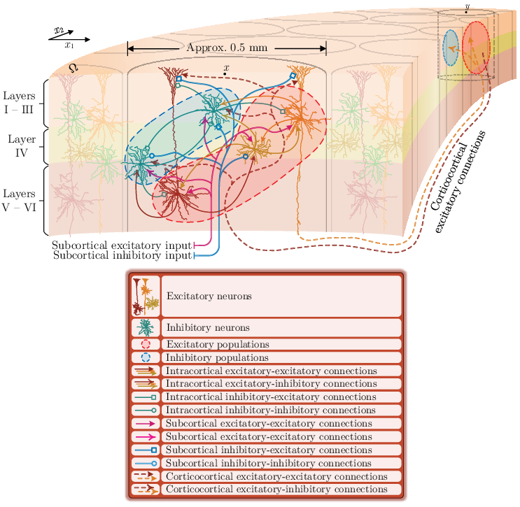
The neocortex has a layered columnar structure consisting mostly of six distinctive layers. Neurons in the neocortex are organized in vertical columns, usually referred to as cortical columns or macrocolumns, which are a fraction of a millimeter wide and traverse all the layers of the neocortex from the white matter to the pial surface [28, 41, 27]. Depending on their type of action, neurons are mainly classified as excitatory or inhibitory, wherein this distinction depends on whether they increase the firing rate in the destination neurons they are communicating with, or they essentially suppress them. Inhibitory neurons are located in all layers and usually have axons that remain within the same area where their cell body resides, and hence, they have a local range of action. Layers III, V, and VI contain pyramidal excitatory neurons whose axons can provide long-range communication (projection) throughout the neocortex. Layer IV contains primarily star-shaped excitatory interneurons that receive sensory inputs from the thalamus. Figure 1 shows a schematic of the structure of the neocortex, including the intracortical and corticocortical neuronal connections; see [28, Ch. 15] for further details.

On a local scale, within a cortical column, neurons are densely interconnected and involve all types of feedforward and feedback intracortical connections. Such a dense and relatively homogeneous local structure of the neocortex suggests modeling a local population of functionally similar neurons by a single space-averaged neuron, which preserves enough physiological information to understand the temporal patterns observed in spatially smoothed (averaged) EEG signals without creating excessive theoretical complicacies in the mathematical analysis of the model. On a global scale, in the exclusively excitatory corticocortical communication throughout the neocortex, two major patterns of connectivity are observed. Namely, a homogeneous, symmetrical, and translation invariant pattern of connections, versus a heterogeneous, patchy, and asymmetrical distribution of connections. For modeling simplicity and due to unavailability of detailed anatomical data, in the model that we investigate in this paper the corticocortical connectivity is assumed to be isotropic, homogeneous, symmetric, and translation invariant [36].

To establish the mathematical framework of the model, let Ω=(0,ω)×(0,ω)\Omega=(0,\omega)\times(0,\omega), ω>0\omega>0, be an open rectangle in ℝ2\mathbb{R}^{2} that defines the domain of the neocortex. Each point x=(x1,x2)∈Ωx=(x_{1},x_{2})\in\Omega indicates the location of a local network—possibly representing a cortical column—modeled by a space-averaged excitatory neuron and a space-averaged inhibitory neuron. Let e denote a population of excitatory neurons and i denote a population of inhibitory neurons. For x∈Ωx\in\Omega, t∈[0,T]t\in[0,T], T>0T>0, and x,y∈{e,i}\textsc{x},\textsc{y}\in\{\textsc{e},\textsc{i}\}, we denote by vx​(x,t)v_{\textsc{x}}(x,t), measured in mV, the spatially mean soma membrane potential of a population of type x centered at xx. Moreover, we denote by ixy​(x,t)i_{\textsc{x}\textsc{y}}(x,t), measured in mV, the spatially mean postsynaptic activation of synapses of a population of type x centered at xx, onto a population of type y centered at the same point xx. In addition, we denote by wex​(x,t)w_{\textsc{e}\textsc{x}}(x,t), measured in s−1\mathrm{s}^{-1}, the mean rate of corticocortical excitatory input pulses from the entire domain of the neocortex to a population of type x centered at xx. Finally, we denote by gxy​(x,t)g_{\textsc{x}\textsc{y}}(x,t), measured in s−1\mathrm{s}^{-1}, the mean rate of subcortical input pulses of type x to a population of type y centered at xx. Note that, by definition, ixy​(x,t)i_{\textsc{x}\textsc{y}}(x,t), wex​(x,t)w_{\textsc{e}\textsc{x}}(x,t), and gxy​(x,t)g_{\textsc{x}\textsc{y}}(x,t) are nonnegative quantities.

Then, as developed in [36], the system of coupled ordinary and partial differential equations

(3.1) (τe∂t+1)ve(x,t)\displaystyle(\tau_{\textsc{e}}\partial_{t}+1)v_{\textsc{e}}(x,t) =Vee−ve​(x,t)|Vee|​iee​(x,t)+Vie−ve​(x,t)|Vie|​iie​(x,t),\displaystyle=\frac{\mathrm{V}_{\textsc{e}\textsc{e}}-v_{\textsc{e}}(x,t)}{|\mathrm{V}_{\textsc{e}\textsc{e}}|}i_{\textsc{e}\textsc{e}}(x,t)+\frac{\mathrm{V}_{\textsc{i}\textsc{e}}-v_{\textsc{e}}(x,t)}{|\mathrm{V}_{\textsc{i}\textsc{e}}|}i_{\textsc{i}\textsc{e}}(x,t),
(τi∂t+1)vi(x,t)\displaystyle(\tau_{\textsc{i}}\partial_{t}+1)v_{\textsc{i}}(x,t) =Vei−vi​(x,t)|Vei|​iei​(x,t)+Vii−vi​(x,t)|Vii|​iii​(x,t),\displaystyle=\frac{\mathrm{V}_{\textsc{e}\textsc{i}}-v_{\textsc{i}}(x,t)}{|\mathrm{V}_{\textsc{e}\textsc{i}}|}i_{\textsc{e}\textsc{i}}(x,t)+\frac{\mathrm{V}_{\textsc{i}\textsc{i}}-v_{\textsc{i}}(x,t)}{|\mathrm{V}_{\textsc{i}\textsc{i}}|}i_{\textsc{i}\textsc{i}}(x,t),
(∂t+γee)2iee(x,t)\displaystyle(\partial_{t}+\gamma_{\textsc{e}\textsc{e}})^{2}i_{\textsc{e}\textsc{e}}(x,t) =e​Υee​γee​[Nee​fe​(ve​(x,t))+wee​(x,t)+gee​(x,t)],\displaystyle=e\Upsilon_{\textsc{e}\textsc{e}}\gamma_{\textsc{e}\textsc{e}}\left[\mathrm{N}_{\textsc{e}\textsc{e}}f_{\textsc{e}}\big(v_{\textsc{e}}(x,t)\big)+w_{\textsc{e}\textsc{e}}(x,t)+g_{\textsc{e}\textsc{e}}(x,t)\right],
(∂t+γei)2iei(x,t)\displaystyle(\partial_{t}+\gamma_{\textsc{e}\textsc{i}})^{2}i_{\textsc{e}\textsc{i}}(x,t) =e​Υei​γei​[Nei​fe​(ve​(x,t))+wei​(x,t)+gei​(x,t)],\displaystyle=e\Upsilon_{\textsc{e}\textsc{i}}\gamma_{\textsc{e}\textsc{i}}\left[\mathrm{N}_{\textsc{e}\textsc{i}}f_{\textsc{e}}\big(v_{\textsc{e}}(x,t)\big)+w_{\textsc{e}\textsc{i}}(x,t)+g_{\textsc{e}\textsc{i}}(x,t)\right],
(∂t+γie)2iie(x,t)\displaystyle(\partial_{t}+\gamma_{\textsc{i}\textsc{e}})^{2}i_{\textsc{i}\textsc{e}}(x,t) =e​Υie​γie​[Nie​fi​(vi​(x,t))+gie​(x,t)],\displaystyle=e\Upsilon_{\textsc{i}\textsc{e}}\gamma_{\textsc{i}\textsc{e}}\left[\mathrm{N}_{\textsc{i}\textsc{e}}f_{\textsc{i}}\big(v_{\textsc{i}}(x,t)\big)+g_{\textsc{i}\textsc{e}}(x,t)\right],
(∂t+γii)2iii(x,t)\displaystyle(\partial_{t}+\gamma_{\textsc{i}\textsc{i}})^{2}i_{\textsc{i}\textsc{i}}(x,t) =e​Υii​γii​[Nii​fi​(vi​(x,t))+gii​(x,t)],\displaystyle=e\Upsilon_{\textsc{i}\textsc{i}}\gamma_{\textsc{i}\textsc{i}}\left[\mathrm{N}_{\textsc{i}\textsc{i}}f_{\textsc{i}}\big(v_{\textsc{i}}(x,t)\big)+g_{\textsc{i}\textsc{i}}(x,t)\right],
[(∂t+νΛee)2−32ν2Δ]wee(x,t)\displaystyle\big[(\partial_{t}+\nu\Lambda_{\textsc{e}\textsc{e}})^{2}-\tfrac{3}{2}\nu^{2}\Delta\big]w_{\textsc{e}\textsc{e}}(x,t) =ν2​Λee2​Mee​fe​(ve​(x,t)),\displaystyle=\nu^{2}\Lambda_{\textsc{e}\textsc{e}}^{2}\mathrm{M}_{\textsc{e}\textsc{e}}f_{\textsc{e}}\big(v_{\textsc{e}}(x,t)\big),
[(∂t+νΛei)2−32ν2Δ]wei(x,t)\displaystyle\big[(\partial_{t}+\nu\Lambda_{\textsc{e}\textsc{i}})^{2}-\tfrac{3}{2}\nu^{2}\Delta\big]w_{\textsc{e}\textsc{i}}(x,t) =ν2​Λei2​Mei​fe​(ve​(x,t)),(x,t)∈Ω×(0,T],\displaystyle=\nu^{2}\Lambda_{\textsc{e}\textsc{i}}^{2}\mathrm{M}_{\textsc{e}\textsc{i}}f_{\textsc{e}}\big(v_{\textsc{e}}(x,t)\big),\hskip 46.94687pt(x,t)\in\Omega\times(0,T],

with periodic boundary conditions provides a mean field model for the electrocortical activity in the neocortex. Here, ee is the Napier constant and fx​(⋅)f_{\textsc{x}}(\cdot) is the mean firing rate function of a population of type x and is given by

(3.2) fx​(vx​(x,t)):=Fx1+exp⁡(−2​vx​(x,t)−μxσx),x∈{e,i}.f_{\textsc{x}}\big(v_{\textsc{x}}(x,t)\big):=\frac{\mathrm{F}_{{\textsc{x}}}}{1+\exp\left(-\sqrt{2}\,\dfrac{v_{\textsc{x}}(x,t)-\mu_{\textsc{x}}}{\sigma_{\textsc{x}}}\right)},\quad\textsc{x}\in\{\textsc{e},\textsc{i}\}.

The definition of the biophysical parameters of the model and the ranges of the values they may take are given in Table 1. For the range of values given in Table 1, we have |Vee|=Vee|\mathrm{V}_{\textsc{e}\textsc{e}}|=\mathrm{V}_{\textsc{e}\textsc{e}}, |Vei|=Vei|\mathrm{V}_{\textsc{e}\textsc{i}}|=\mathrm{V}_{\textsc{e}\textsc{i}}, |Vie|=−Vie|\mathrm{V}_{\textsc{i}\textsc{e}}|=-\mathrm{V}_{\textsc{i}\textsc{e}} , and |Vii|=−Vii|\mathrm{V}_{\textsc{i}\textsc{i}}|=-\mathrm{V}_{\textsc{i}\textsc{i}}, which we use to simplify (3.1). Note that other than notational changes to the original equations given in [36], we have changed the reference of electric potential to the resting potential to avoid the constant terms that would otherwise appear in (3.1). Figure 2 shows a schematic of intracortical, corticocortical, and subcortical inputs to two local networks located at points xx and yy, along with their contribution to the global corticocortical activation as modeled by (3.1). The particular coupling between the equations of the model is depicted by the block diagram shown in Figure 3.

Table 1: Definition and range of values for the biophysical parameters of the mean field model (3.1). All electric potentials are given with respect to the mean resting soma membrane potential vrest=−70​ mVv_{\rm rest}=-70\text{ mV} [3].
Parameter Definition Range Unit
τe\tau_{\textsc{e}} Passive excitatory membrane decay time constant [0.005,0.15][0.005,0.15] s
τi\tau_{\textsc{i}} Passive inhibitory membrane decay time constant [0.005,0.15][0.005,0.15] s
Vee\mathrm{V}_{\textsc{e}\textsc{e}}, Vei\mathrm{V}_{\textsc{e}\textsc{i}} Mean excitatory Nernst potentials [50,80][50,80] mV
Vie\mathrm{V}_{\textsc{i}\textsc{e}}, Vii\mathrm{V}_{\textsc{i}\textsc{i}} Mean inhibitory Nernst potentials [−20,−5][-20,-5] mV
γee\gamma_{\textsc{e}\textsc{e}}, γei\gamma_{\textsc{e}\textsc{i}} Excitatory postsynaptic potential rate constants [100,1000][100,1000] s-1
γie\gamma_{\textsc{i}\textsc{e}}, γii\gamma_{\textsc{i}\textsc{i}} Inhibitory postsynaptic potential rate constants [10,500][10,500] s-1
Υee\Upsilon_{\textsc{e}\textsc{e}}, Υei\Upsilon_{\textsc{e}\textsc{i}} Amplitude of excitatory postsynaptic potentials [0.1,2.0][0.1,2.0] mV
Υie\Upsilon_{\textsc{i}\textsc{e}}, Υii\Upsilon_{\textsc{i}\textsc{i}} Amplitude of inhibitory postsynaptic potentials [0.1,2.0][0.1,2.0] mV
Nee\mathrm{N}_{\textsc{e}\textsc{e}}, Nei\mathrm{N}_{\textsc{e}\textsc{i}} Number of intracortical excitatory connections [2000,5000][2000,5000] —
Nie\mathrm{N}_{\textsc{i}\textsc{e}}, Nii\mathrm{N}_{\textsc{i}\textsc{i}} Number of intracortical inhibitory connections [100,1000][100,1000] —
ν\nu Corticocortical conduction velocity [100,1000][100,1000] cm/s
Λee\Lambda_{\textsc{e}\textsc{e}}, Λei\Lambda_{\textsc{e}\textsc{i}} Decay scale of corticocortical excitatory connectivities [0.1,1.0][0.1,1.0] cm-1
Mee\mathrm{M}_{\textsc{e}\textsc{e}}, Mei\mathrm{M}_{\textsc{e}\textsc{i}} Number of corticocortical excitatory connections [2000,5000][2000,5000] —
Fe\mathrm{F}_{{\textsc{e}}} Maximum mean excitatory firing rate [50,500][50,500] s-1
Fi\mathrm{F}_{{\textsc{i}}} Maximum mean inhibitory firing rate [50,500][50,500] s-1
μe\mu_{\textsc{e}} Excitatory firing threshold potential [15,30][15,30] mV
μi\mu_{\textsc{i}} Inhibitory firing threshold potential [15,30][15,30] mV
σe\sigma_{\textsc{e}} Standard deviation of excitatory firing threshold potential [2,7][2,7] mV
σi\sigma_{\textsc{i}} Standard deviation of inhibitory firing threshold potential [2,7][2,7] mV
Refer to caption
Figure 2: Cortical inputs to two local networks located at points xx and yy as modeled by (3.1).
Refer to caption
Figure 3: Block diagram of the mean field model (3.1). The operators P1,…,P8P_{1},\dots,P_{8} represent the eight equations in (3.1), respectively. Similar to Figures 1 and 2, the blocks associated with excitatory populations are shown in red, and the blocks associated with inhibitory populations are shown in blue.

The first two equations in (3.1), that is, the vv-equations, model the dynamics of the resistive-capacitive membrane of the space-averaged neurons located at xx. In the absence of postsynaptic ii-inputs, the mean membrane potential decays exponentially to the resting potential. The fractions appearing in the equations weight the postsynaptic inputs to incorporate the effect of transmembrane diffusive ion flows into the model. Specifically, the depolarizing effect of excitatory inputs on the membrane is linearly decreased by the weights as the membrane potential rises to the Nernst (reversal) potential. When the membrane potential exceeds the Nernst potential, the effect is reversed and further excitation tends to hyperpolarize the membrane. The weights associated with the inhibitory postsynaptic inputs have opposite signs at the resting potential, and hence, they have an opposite reversal effect.

The critically damped second order dynamics of the four ii-equations in (3.1) generates a synaptic α\alpha-function—as in the classical dendritic cable theory—in response to an impulse. As shown in Figure 2, these second order dynamical systems are driven by three different sources of presynaptic spikes, namely, the inputs Nxy​fx​(vx)\mathrm{N}_{\textsc{x}\textsc{y}}f_{\textsc{x}}(v_{\textsc{x}}) from local neuronal populations, the excitatory inputs wexw_{\textsc{e}\textsc{x}} form corticocortical fibers, and the inputs gxyg_{\textsc{x}\textsc{y}} from subcortical regions. As a result, these four equations generate the postsynaptic responses that modulate the polarization of the cell membranes according to the vv-equations discussed before.

Unlike the conduction through short-range intracortical fibers, the conduction through long-range corticocortical fibers cannot be assumed to be instantaneous. The ww-equations in (3.1) form a system of telegraph equations that effectively models the propagation of the excitatory axonal pulses through corticocortical fibers. To derive these equations, it is assumed in [36] that the strength of corticocortical connections onto a local population decays exponentially with distance, with the characteristic scale Λex\Lambda_{\textsc{e}\textsc{x}}. Moreover, it is assumed that the spatial distribution of connections is isotropic and homogeneous all over the neocortex.

In practical applications, the key variable in the model presented by (3.1) is the mean membrane potential of excitatory populations ve​(x,t)v_{\textsc{e}}(x,t) that is presumed to be linearly proportional to EEG recordings from the scalp [36, 37]. For further details of the model see [36], or the introductory sections of [6, 37, 21].

Now, let

v⁡(x,t)\displaystyle v(x,t) :=(ve​(x,t),vi​(x,t))∈ℝ2,\displaystyle:=\big(v_{\textsc{e}}(x,t),v_{\textsc{i}}(x,t)\big)\in\mathbb{R}^{2},
i⁡(x,t)\displaystyle i(x,t) :=(iee​(x,t),iei​(x,t),iie​(x,t),iii​(x,t))∈ℝ4,\displaystyle:=\big(i_{\textsc{e}\textsc{e}}(x,t),i_{\textsc{e}\textsc{i}}(x,t),i_{\textsc{i}\textsc{e}}(x,t),i_{\textsc{i}\textsc{i}}(x,t)\big)\in\mathbb{R}^{4},
w⁡(x,t)\displaystyle w(x,t) :=(wee​(x,t),wei​(x,t))∈ℝ2,\displaystyle:=\big(w_{\textsc{e}\textsc{e}}(x,t),w_{\textsc{e}\textsc{i}}(x,t)\big)\in\mathbb{R}^{2},
g⁡(x,t)\displaystyle g(x,t) :=(gee​(x,t),gei​(x,t),gie​(x,t),gii​(x,t))∈ℝ4,\displaystyle:=\big(g_{\textsc{e}\textsc{e}}(x,t),g_{\textsc{e}\textsc{i}}(x,t),g_{\textsc{i}\textsc{e}}(x,t),g_{\textsc{i}\textsc{i}}(x,t)\big)\in\mathbb{R}^{4},

and note that (3.1) can be represented in vector form in Ω×(0,T]\Omega\times(0,T] as

(3.3) Φ​∂tv+v−J1​i+J2​v​iT​Ψ​J4+J3​v​iT​Ψ​J5\displaystyle\Phi\partial_{t}v+v-J_{1}i+J_{2}vi^{\mathrm{T}}\Psi J_{4}+J_{3}vi^{\mathrm{T}}\Psi J_{5} =0,\displaystyle=0,
(3.4) ∂t2i+2​Γ​∂ti+Γ2​i−e​Υ​Γ​J6​w−e​Υ​Γ​N​J7​f​(v)\displaystyle\partial_{t}^{2}i+2\Gamma\partial_{t}i+\Gamma^{2}i-e\Upsilon\Gamma J_{6}w-e\Upsilon\Gamma\mathrm{N}J_{7}f(v) =e​Υ​Γ​g,\displaystyle=e\Upsilon\Gamma g,
(3.5) ∂t2w+2​ν​Λ​∂tw−32​ν2​Δ​w+ν2​Λ2​w−ν2​Λ2​M​J8​f​(v)\displaystyle\partial_{t}^{2}w+2\nu\Lambda\partial_{t}w-\tfrac{3}{2}\nu^{2}\Delta w+\nu^{2}\Lambda^{2}w-\nu^{2}\Lambda^{2}\mathrm{M}J_{8}f\big(v\big) =0,\displaystyle=0,

where vv, ii, and ww are Ω\Omega-periodic vector-valued functions with the initial values

(3.6) v|t=0=v0,i|t=0=i0,(∂ti)|t=0=i0′,w|t=0=w0,(∂tw)|t=0=w0′,v\big|_{t=0}=v_{0},\quad i\big|_{t=0}=i_{0},\quad(\partial_{t}i)\big|_{t=0}=i_{0}^{\prime},\quad w\big|_{t=0}=w_{0},\quad(\partial_{t}w)\big|_{t=0}=w_{0}^{\prime},

and

(3.7) Φ\displaystyle\Phi =diag⁡(τe,τi),\displaystyle=\mathrm{diag}\big(\tau_{\textsc{e}},\tau_{\textsc{i}}\big),\quad Ψ\displaystyle\Psi =diag⁡(1|Vee|,1|Vei|,1|Vie|,1|Vii|),\displaystyle=\mathrm{diag}\big(\tfrac{1}{|\mathrm{V}_{\textsc{e}\textsc{e}}|},\tfrac{1}{|\mathrm{V}_{\textsc{e}\textsc{i}}|},\tfrac{1}{|\mathrm{V}_{\textsc{i}\textsc{e}}|},\tfrac{1}{|\mathrm{V}_{\textsc{i}\textsc{i}}|}\big),
Γ\displaystyle\Gamma =diag⁡(γee,γei,γie,γii),\displaystyle=\mathrm{diag}(\gamma_{\textsc{e}\textsc{e}},\gamma_{\textsc{e}\textsc{i}},\gamma_{\textsc{i}\textsc{e}},\gamma_{\textsc{i}\textsc{i}}),\quad Υ\displaystyle\Upsilon =diag⁡(Υee,Υei,Υie,Υii),\displaystyle=\mathrm{diag}(\Upsilon_{\textsc{e}\textsc{e}},\Upsilon_{\textsc{e}\textsc{i}},\Upsilon_{\textsc{i}\textsc{e}},\Upsilon_{\textsc{i}\textsc{i}}),
N\displaystyle\mathrm{N} =diag⁡(Nee,Nei,Nie,Nii),\displaystyle=\mathrm{diag}(\mathrm{N}_{\textsc{e}\textsc{e}},\mathrm{N}_{\textsc{e}\textsc{i}},\mathrm{N}_{\textsc{i}\textsc{e}},\mathrm{N}_{\textsc{i}\textsc{i}}),\quad M\displaystyle\mathrm{M} =diag⁡(Mee,Mei),\displaystyle=\mathrm{diag}(\mathrm{M}_{\textsc{e}\textsc{e}},\mathrm{M}_{\textsc{e}\textsc{i}}),
Λ\displaystyle\Lambda =diag⁡(Λee,Λei),\displaystyle=\mathrm{diag}(\Lambda_{\textsc{e}\textsc{e}},\Lambda_{\textsc{e}\textsc{i}}),\quad J1\displaystyle J_{1} =[I2×2−I2×2],\displaystyle=\left[\begin{array}[]{cc}I_{2\times 2}&-I_{2\times 2}\end{array}\right],
J2\displaystyle J_{2} =diag⁡(1,0),\displaystyle=\mathrm{diag}(1,0),\quad J3\displaystyle J_{3} =diag⁡(0,1),\displaystyle=\mathrm{diag}(0,1),
J4\displaystyle J_{4} =[1010]T,\displaystyle=\left[\begin{array}[]{cccc}1&0&1&0\end{array}\right]^{\mathrm{T}},\quad J5\displaystyle J_{5} =[0101]T,\displaystyle=\left[\begin{array}[]{cccc}0&1&0&1\end{array}\right]^{\mathrm{T}},
J6\displaystyle J_{6} =[10000100]T,\displaystyle=\left[\begin{array}[]{cccc}1&0&0&0\\ 0&1&0&0\end{array}\right]^{\mathrm{T}},\quad J7\displaystyle J_{7} =[11000011]T,\displaystyle=\left[\begin{array}[]{cccc}1&1&0&0\\ 0&0&1&1\end{array}\right]^{\mathrm{T}},
J8\displaystyle J_{8} =[1010],\displaystyle=\left[\begin{array}[]{cc}1&0\\ 1&0\end{array}\right],\quad f⁡(v)\displaystyle f(v) =[fe​([10]​v)fi​([01]​v)].\displaystyle=\left[\begin{array}[]{c}f_{\textsc{e}}\big(\left[\begin{array}[]{cc}1&0\\ \end{array}\right]v\big)\\ f_{\textsc{i}}\big(\left[\begin{array}[]{cc}0&1\\ \end{array}\right]v\big)\end{array}\right].

For simplicity of exposition, the dependence of the functions vv, ii, ww, and gg on the arguments (x,t)(x,t) is not explicitly shown in (3.3)–(3.5). Note that (3.3) and (3.4), which model the local dynamics of the neocortex, are essentially systems of ordinary differential equations. These equations do not possess any spatial smoothing component, and hence, their solutions are expected to evolve in less regular function spaces [47, 39]. The system of partial differential equations (3.5) consists of two telegraph equations coupled indirectly through (3.3) and (3.4); see Figure 3.

Remark 3.1 (Variations in the parameters).

: In the analysis that follows in the rest of the paper, we assume that all the parameters of the model are constant. However, in practical applications, certain parameters may be considered to vary in time or space to model specific physiological situations in the brain. The variations can occur independently, or can be modeled using additional ODE’s or PDE’s coupled with the existing equations. We give all the details of the results—even though some of which may be found fairly standard—along with a careful inclusion of all parameters. Therefore, in applications, it should be possible to easily observe where the parameters of interest appear in the analysis, and whether or not their particular variations can affect the validity of the results.

4 Existence and Uniqueness of Solutions

In this section, we investigate the problem of existence, uniqueness, and regularity of solutions for (3.3)–(3.5) with the initial values (3.6) and periodic boundary conditions. We set appropriate spaces of Ω\Omega-periodic functions as the functional framework of the problem by which we include the boundary conditions in the solution spaces. We view v⁡(x,t)v(x,t), i⁡(x,t)i(x,t), and w⁡(x,t)w(x,t) as Banach space-valued functions and follow the standard technique of Galerkin approximations [44, 16, 51] to construct weak and strong solutions in Theorems 4.5 and 4.7. The details of the proof of these results can be skipped in the case the reader is proficient in the analysis of Galerkin method.

First, define the function spaces

(4.1) ℒv2\displaystyle\mathcal{L}^{2}_{v} :=Lper2​(Ω,ℝ2),\displaystyle:=L_{\rm per}^{2}(\Omega;\mathbb{R}^{2}), ℒi2\displaystyle\quad\mathcal{L}^{2}_{i} :=Lper2​(Ω,ℝ4),\displaystyle:=L_{\rm per}^{2}(\Omega;\mathbb{R}^{4}), ℒw2\displaystyle\quad\mathcal{L}^{2}_{w} :=Lper2​(Ω,ℝ2),\displaystyle:=L_{\rm per}^{2}(\Omega;\mathbb{R}^{2}),
ℒv∞\displaystyle\mathcal{L}^{\infty}_{v} :=Lper∞​(Ω,ℝ2),\displaystyle:=L_{\rm per}^{\infty}(\Omega;\mathbb{R}^{2}), ℒi∞\displaystyle\quad\mathcal{L}^{\infty}_{i} :=Lper∞​(Ω,ℝ4),\displaystyle:=L_{\rm per}^{\infty}(\Omega;\mathbb{R}^{4}), ℒw∞\displaystyle\quad\mathcal{L}^{\infty}_{w} :=Lper∞​(Ω,ℝ2),\displaystyle:=L_{\rm per}^{\infty}(\Omega;\mathbb{R}^{2}),
ℋw1\displaystyle\mathcal{H}_{w}^{1} :=Hper1​(Ω,ℝ2),\displaystyle:=H_{\rm per}^{1}(\Omega;\mathbb{R}^{2}), ℋw2\displaystyle\quad\mathcal{H}_{w}^{2} :=Hper2​(Ω,ℝ2),\displaystyle:=H_{\rm per}^{2}(\Omega;\mathbb{R}^{2}),
ℒ∂w2\displaystyle\mathcal{L}_{\partial w}^{2} :=Lper2​(Ω,ℝ2×2),\displaystyle:=L_{\rm per}^{2}(\Omega;\mathbb{R}^{2\times 2}), ℋ∂w1\displaystyle\quad\mathcal{H}_{\partial w}^{1} :=Hper1​(Ω,ℝ2×2),\displaystyle:=H_{\rm per}^{1}(\Omega;\mathbb{R}^{2\times 2}),
𝒲w1,∞\displaystyle\mathcal{W}_{w}^{1,\infty} :=Wper1,∞​(Ω,ℝ2),\displaystyle:=W_{\rm per}^{1,\infty}(\Omega;\mathbb{R}^{2}),

and denote by ℒv2∗{\mathcal{L}^{2}_{v}}^{\ast}, ℒi2∗{\mathcal{L}^{2}_{i}}^{\ast}, and ℋw1∗{\mathcal{H}^{1}_{w}}^{\!\!\ast} the dual spaces of ℒv2\mathcal{L}^{2}_{v}, ℒi2\mathcal{L}^{2}_{i}, and ℋw1\mathcal{H}_{w}^{1}, respectively. Note that ℒv2\mathcal{L}^{2}_{v} and ℒi2\mathcal{L}^{2}_{i} are, respectively, isometrically isomorphic to ℒv2∗{\mathcal{L}^{2}_{v}}^{\ast} and ℒi2∗{\mathcal{L}^{2}_{i}}^{\ast} [18, Th. 6.15], which we denote by ℒv2∗=ℒv2{\mathcal{L}^{2}_{v}}^{\ast}=\mathcal{L}^{2}_{v} and ℒi2∗=ℒi2{\mathcal{L}^{2}_{i}}^{\ast}=\mathcal{L}^{2}_{i}. By the Rellich-Kondrachov compact embedding theorems we have ℋw1⋐ℒw2↪ℋw1∗\mathcal{H}_{w}^{1}\Subset\mathcal{L}^{2}_{w}\hookrightarrow{\mathcal{H}^{1}_{w}}^{\!\!\ast}; see [9, Th. 6.6-3] and [44, Th. A.4]. Moreover, there exists a dual orthogonal basis of ℋw1\mathcal{H}_{w}^{1} and ℒw2\mathcal{L}_{w}^{2} given by the following lemma. The proof of this lemma is fairly standard and follows the general results given in [51, Sec. II.2.1].

Lemma 4.1 (Dual orthogonal basis).

There exists an orthonormal basis of ℒw2\mathcal{L}^{2}_{w} that is also an orthogonal basis of ℋw1\mathcal{H}_{w}^{1}, and can be constructed by the eigenfunctions of the linear operator A:=−Δ+IA:=-\Delta+I.

Now, before proceeding to the main results of this section, we define the notions of weak and strong solutions of (3.3)–(3.6) as used in this paper.

Definition 4.2 (Weak solution).

A solution (v,i,w)(v,i,w) is called an Ω\Omega-periodic weak solution of the initial value problem (3.3)–(3.6) if it solves the weak version of the problem wherein the partial differential equations are understood as equalities in the space of duals L2​(0,T,ℒv2∗×ℒi2∗×ℋw1∗)L^{2}(0,T;{\mathcal{L}^{2}_{v}}^{\ast}\times{\mathcal{L}^{2}_{i}}^{\ast}\times{\mathcal{H}^{1}_{w}}^{\!\!\ast}). That is, the functions

v∈L2​(0,T,ℒv2),i∈L2​(0,T,ℒi2),w∈L2​(0,T,ℋw1),v\in L^{2}(0,T;\mathcal{L}_{v}^{2}),\quad i\in L^{2}(0,T;\mathcal{L}_{i}^{2}),\quad w\in L^{2}(0,T;\mathcal{H}_{w}^{1}),

with

dt​v\displaystyle\mathrm{d}_{t}v ∈L2​(0,T,ℒv2∗),\displaystyle\in L^{2}(0,T;{\mathcal{L}^{2}_{v}}^{\ast}),\quad dt​i\displaystyle\mathrm{d}_{t}i ∈L2​(0,T,ℒi2),\displaystyle\in L^{2}(0,T;\mathcal{L}_{i}^{2}),\quad dt2​i∈L2​(0,T,ℒi2∗),\displaystyle\mathrm{d}_{t}^{2}i\in L^{2}(0,T;{\mathcal{L}^{2}_{i}}^{\ast}),
dt​w\displaystyle\mathrm{d}_{t}w ∈L2​(0,T,ℒw2),\displaystyle\in L^{2}(0,T;\mathcal{L}_{w}^{2}),\quad dt2​w\displaystyle\mathrm{d}_{t}^{2}w ∈L2​(0,T,ℋw1∗),\displaystyle\in L^{2}(0,T;{\mathcal{H}^{1}_{w}}^{\!\!\ast}),

construct an Ω\Omega-periodic weak solution for (3.3)–(3.6) if for every ℓv∈ℒv2\ell_{v}\in\mathcal{L}_{v}^{2}, ℓi∈ℒi2\ell_{i}\in\mathcal{L}_{i}^{2}, hw∈ℋw1h_{w}\in\mathcal{H}_{w}^{1}, and almost every t∈[0,T]t\in[0,T], T>0T>0,

(4.2) ⟨Φ​dt​v,ℓv⟩ℒv2+(v,ℓv)ℒv2−(J1​i,ℓv)ℒv2+(J2​v​iT​Ψ​J4+J3​v​iT​Ψ​J5,ℓv)ℒv2\displaystyle\big\langle\Phi\mathrm{d}_{t}v,\ell_{v}\big\rangle\hskip-0.85358pt_{\mathcal{L}_{v}^{2}}+\big(v,\ell_{v}\big)\hskip-0.85358pt_{\mathcal{L}_{v}^{2}}-\big(J_{1}i,\ell_{v}\big)\hskip-0.85358pt_{\mathcal{L}_{v}^{2}}+\big(J_{2}vi^{\mathrm{T}}\Psi J_{4}+J_{3}vi^{\mathrm{T}}\Psi J_{5},\ell_{v}\big)\hskip-0.85358pt_{\mathcal{L}_{v}^{2}} =0,\displaystyle=0,
(4.3) ⟨dt2​i,ℓi⟩ℒi2+2​(Γ​dt​i,ℓi)ℒi2+(Γ2​i,ℓi)ℒi2−e​(Υ​Γ​J6​w,ℓi)ℒi2\displaystyle\big\langle\mathrm{d}_{t}^{2}i,\ell_{i}\big\rangle\hskip-0.85358pt_{\mathcal{L}_{i}^{2}}+2\big(\Gamma\mathrm{d}_{t}i,\ell_{i}\big)\hskip-0.85358pt_{\mathcal{L}_{i}^{2}}+\big(\Gamma^{2}i,\ell_{i}\big)\hskip-0.85358pt_{\mathcal{L}_{i}^{2}}-e\big(\Upsilon\Gamma J_{6}w,\ell_{i}\big)\hskip-0.85358pt_{\mathcal{L}_{i}^{2}}\hskip 62.0268pt
−e​(Υ​Γ​N​J7​f​(v),ℓi)ℒi2\displaystyle-e\big(\Upsilon\Gamma\mathrm{N}J_{7}f(v),\ell_{i}\big)\hskip-0.85358pt_{\mathcal{L}_{i}^{2}} =e​(Υ​Γ​g,ℓi)ℒi2,\displaystyle=e\big(\Upsilon\Gamma g,\ell_{i}\big)\hskip-0.85358pt_{\mathcal{L}_{i}^{2}},
(4.4) ⟨dt2​w,hw⟩ℋw1+2​ν​(Λ​dt​w,hw)ℒw2+32​ν2​(∂xw,∂xhw)ℒ∂w2\displaystyle\big\langle\mathrm{d}_{t}^{2}w,h_{w}\big\rangle\hskip-0.85358pt_{\mathcal{H}_{w}^{1}}+2\nu\big(\Lambda\mathrm{d}_{t}w,h_{w}\big)\hskip-0.85358pt_{\mathcal{L}_{w}^{2}}+\tfrac{3}{2}\nu^{2}\big(\partial_{x}w,\partial_{x}h_{w}\big)\hskip-0.85358pt_{\mathcal{L}_{\partial w}^{2}}\hskip 71.98543pt
+ν2​(Λ2​w,hw)ℒw2−ν2​(Λ2​M​J8​f​(v),hw)ℒw2\displaystyle+\nu^{2}\big(\Lambda^{2}w,h_{w}\big)\hskip-0.85358pt_{\mathcal{L}_{w}^{2}}-\nu^{2}\big(\Lambda^{2}\mathrm{M}J_{8}f(v),h_{w}\big)\hskip-0.85358pt_{\mathcal{L}_{w}^{2}} =0,\displaystyle=0,

with the initial values

(4.5) v⁡(0)=v0,i⁡(0)=i0,dt​i​(0)=i0′,w⁡(0)=w0,dt​w​(0)=w0′.v(0)=v_{0},\quad i(0)=i_{0},\quad\mathrm{d}_{t}i(0)=i_{0}^{\prime},\quad w(0)=w_{0},\quad\mathrm{d}_{t}w(0)=w_{0}^{\prime}.

Definition 4.3 (Strong solution).

A solution (v,i,w)(v,i,w) is called an Ω\Omega-periodic strong solution of the initial value problem (3.3)–(3.6) if it solves the strong version of the problem wherein the partial differential equations are understood as equalities in L2​(0,T,ℒv2×ℒi2×ℒw2)L^{2}(0,T;\mathcal{L}^{2}_{v}\times\mathcal{L}^{2}_{i}\times\mathcal{L}^{2}_{w}). That is, the functions

v∈H1​(0,T,ℒv2),i∈H2​(0,T,ℒi2),w∈L2​(0,T,ℋw2),v\in H^{1}(0,T;\mathcal{L}_{v}^{2}),\quad i\in H^{2}(0,T;\mathcal{L}_{i}^{2}),\quad w\in L^{2}(0,T;\mathcal{H}_{w}^{2}),

with

dt​v\displaystyle\mathrm{d}_{t}v ∈L2​(0,T,ℒv2),\displaystyle\in L^{2}(0,T;\mathcal{L}_{v}^{2}), dt​i\displaystyle\quad\mathrm{d}_{t}i ∈H1​(0,T,ℒi2),\displaystyle\in H^{1}(0,T;\mathcal{L}_{i}^{2}), dt2​i\displaystyle\quad\mathrm{d}_{t}^{2}i ∈L2​(0,T,ℒi2),\displaystyle\in L^{2}(0,T;\mathcal{L}_{i}^{2}),
dt​w\displaystyle\mathrm{d}_{t}w ∈L2​(0,T,ℋw1),\displaystyle\in L^{2}(0,T;\mathcal{H}_{w}^{1}), dt2​w\displaystyle\quad\mathrm{d}_{t}^{2}w ∈L2​(0,T,ℒw2),\displaystyle\in L^{2}(0,T;\mathcal{L}_{w}^{2}),

construct an Ω\Omega-periodic strong solution for (3.3)–(3.6) wherein they solve the equations for almost every x∈Ωx\in\Omega and almost every t∈[0,T]t\in[0,T], T>0T>0.

Now, let ℬv={ℓv(l)}l=1∞\mathcal{B}_{v}=\big\{\ell_{v}^{(l)}\big\}_{l=1}^{\infty} be a basis of ℒv2\mathcal{L}_{v}^{2} such that {Φ12​ℓv(l)}l=1∞\big\{\Phi^{\frac{1}{2}}\ell_{v}^{(l)}\big\}_{l=1}^{\infty} is orthonormal in ℒv2\mathcal{L}_{v}^{2}. Note that (3.7), with the range of values given in Table 1, implies that Φ\Phi is a positive-definite diagonal matrix, and hence, such a basis exists. Moreover, let ℬi={ℓi(l)}l=1∞\mathcal{B}_{i}=\big\{\ell_{i}^{(l)}\big\}_{l=1}^{\infty} be an orthonormal basis of ℒi2\mathcal{L}_{i}^{2}, and ℬw={hw(l)}l=1∞\mathcal{B}_{w}=\big\{h_{w}^{(l)}\big\}_{l=1}^{\infty} be an orthogonal basis of ℋw1\mathcal{H}_{w}^{1} that is orthonormal in ℒw2\mathcal{L}_{w}^{2}; see Lemma 4.1 for the existence and structure of ℬw\mathcal{B}_{w}. Finally, construct the set ℬ={b(k)}k=1∞⊂ℒv2×ℒi2×ℋw1\mathcal{B}=\big\{b^{(k)}\big\}_{k=1}^{\infty}\subset\mathcal{L}^{2}_{v}\times\mathcal{L}^{2}_{i}\times\mathcal{H}_{w}^{1} as

(4.6) ℬ:=ℬv×ℬi×ℬw={b(k)=(ℓv(k),ℓi(k),hw(k)):ℓv(k)∈ℬv,ℓi(k)∈ℬi,hw(k)∈ℬw}k=1∞.\displaystyle\mathcal{B}:=\mathcal{B}_{v}\times\mathcal{B}_{i}\times\mathcal{B}_{w}=\left\{b^{(k)}=(\ell_{v}^{(k)},\ell_{i}^{(k)},h_{w}^{(k)}):\ell_{v}^{(k)}\in\mathcal{B}_{v},\ell_{i}^{(k)}\in\mathcal{B}_{i},h_{w}^{(k)}\in\mathcal{B}_{w}\right\}_{k=1}^{\infty}.

For each positive integer mm, we seek approximations v(m):[0,T]→ℒv2v^{(m)}:[0,T]\rightarrow\mathcal{L}_{v}^{2}, i(m):[0,T]→ℒi2i^{(m)}:[0,T]\rightarrow\mathcal{L}_{i}^{2}, and w(m):[0,T]→ℋw1w^{(m)}:[0,T]\rightarrow\mathcal{H}_{w}^{1} of the form

(4.7) v(m)​(t)\displaystyle v^{(m)}(t) :=∑k=1mcvk(m)​(t)​ℓv(k),\displaystyle:=\sum\nolimits_{k=1}^{m}c_{v_{k}}^{(m)}(t)\ell_{v}^{(k)},
(4.8) i(m)​(t)\displaystyle i^{(m)}(t) :=∑k=1mcik(m)​(t)​ℓi(k),\displaystyle:=\sum\nolimits_{k=1}^{m}c_{i_{k}}^{(m)}(t)\ell_{i}^{(k)},
(4.9) w(m)​(t)\displaystyle w^{(m)}(t) :=∑k=1mcwk(m)​(t)​hw(k),\displaystyle:=\sum\nolimits_{k=1}^{m}c_{w_{k}}^{(m)}(t)h_{w}^{(k)},

constructed by the first mm components of ℬ\mathcal{B} and sufficiently smooth scalar-valued functions cvk(m)c_{v_{k}}^{(m)}, cik(m)c_{i_{k}}^{(m)}, and cwk(m)c_{w_{k}}^{(m)} on [0,T][0,T], such that these approximations satisfy

(4.10) (Φ​dt​v(m),ℓv(k))ℒv2+(v(m),ℓv(k))ℒv2−(J1​i(m),ℓv(k))ℒv2\displaystyle\big(\Phi\mathrm{d}_{t}v^{(m)},\ell_{v}^{(k)}\big)\hskip-0.85358pt_{\mathcal{L}_{v}^{2}}+\big(v^{(m)},\ell_{v}^{(k)}\big)\hskip-0.85358pt_{\mathcal{L}_{v}^{2}}-\big(J_{1}i^{(m)},\ell_{v}^{(k)}\big)\hskip-0.85358pt_{\mathcal{L}_{v}^{2}}\hskip 73.40816pt
+(J2​v(m)​i(m)T​Ψ​J4+J3​v(m)​i(m)T​Ψ​J5,ℓv(k))ℒv2\displaystyle+\big(J_{2}v^{(m)}i^{{(m)}^{\mathrm{T}}}\Psi J_{4}+J_{3}v^{(m)}i^{{(m)}^{\mathrm{T}}}\Psi J_{5},\ell_{v}^{(k)}\big)\hskip-0.85358pt_{\mathcal{L}_{v}^{2}} =0,\displaystyle=0,
(4.11) (dt2​i(m),ℓi(k))ℒi2+2​(Γ​dt​i(m),ℓi(k))ℒi2+(Γ2​i(m),ℓi(k))ℒi2\displaystyle\big(\mathrm{d}_{t}^{2}i^{(m)},\ell_{i}^{(k)}\big)\hskip-0.85358pt_{\mathcal{L}_{i}^{2}}+2\big(\Gamma\mathrm{d}_{t}i^{(m)},\ell_{i}^{(k)}\big)\hskip-0.85358pt_{\mathcal{L}_{i}^{2}}+\big(\Gamma^{2}i^{(m)},\ell_{i}^{(k)}\big)\hskip-0.85358pt_{\mathcal{L}_{i}^{2}}\hskip 62.88077pt
−e​(Υ​Γ​J6​w(m),ℓi(k))ℒi2−e​(Υ​Γ​N​J7​f​(v(m)),ℓi(k))ℒi2\displaystyle-e\big(\Upsilon\Gamma J_{6}w^{(m)},\ell_{i}^{(k)}\big)\hskip-0.85358pt_{\mathcal{L}_{i}^{2}}-e\big(\Upsilon\Gamma\mathrm{N}J_{7}f(v^{(m)}),\ell_{i}^{(k)}\big)\hskip-0.85358pt_{\mathcal{L}_{i}^{2}} =e​(Υ​Γ​g,ℓi(k))ℒi2,\displaystyle=e\big(\Upsilon\Gamma g,\ell_{i}^{(k)}\big)\hskip-0.85358pt_{\mathcal{L}_{i}^{2}},
(4.12) (dt2​w(m),hw(k))ℒw2+2​ν​(Λ​dt​w(m),hw(k))ℒw2+32​ν2​(∂xw(m),∂xhw(k))ℒ∂w2\displaystyle\big(\mathrm{d}_{t}^{2}w^{(m)},h_{w}^{(k)}\big)\hskip-0.85358pt_{\mathcal{L}_{w}^{2}}+2\nu\big(\Lambda\mathrm{d}_{t}w^{(m)},h_{w}^{(k)}\big)\hskip-0.85358pt_{\mathcal{L}_{w}^{2}}+\tfrac{3}{2}\nu^{2}\big(\partial_{x}w^{(m)},\partial_{x}h_{w}^{(k)}\big)\hskip-0.85358pt_{\mathcal{L}_{\partial w}^{2}}\hskip 0.0pt
+ν2​(Λ2​w(m),hw(k))ℒw2−ν2​(Λ2​M​J8​f​(v(m)),hw(k))ℒw2\displaystyle+\nu^{2}\big(\Lambda^{2}w^{(m)},h_{w}^{(k)}\big)\hskip-0.85358pt_{\mathcal{L}_{w}^{2}}-\nu^{2}\big(\Lambda^{2}\mathrm{M}J_{8}f(v^{(m)}),h_{w}^{(k)}\big)\hskip-0.85358pt_{\mathcal{L}_{w}^{2}} =0,\displaystyle=0,

for all t∈[0,T]t\in[0,T] and k=1,…,mk=1,\dots,m, subject to the initial conditions

(4.13) cvk(m)​(0)\displaystyle c_{v_{k}}^{(m)}(0) =(v0,ℓv(k))ℒv2,\displaystyle=\big(v_{0},\ell_{v}^{(k)}\big)\hskip-0.85358pt_{\mathcal{L}_{v}^{2}}, cik(m)​(0)\displaystyle\quad c_{i_{k}}^{(m)}(0) =(i0,ℓi(k))ℒi2,\displaystyle=\big(i_{0},\ell_{i}^{(k)}\big)\hskip-0.85358pt_{\mathcal{L}_{i}^{2}}, dt​cik(m)​(0)\displaystyle\quad\mathrm{d}_{t}c_{i_{k}}^{(m)}(0) =(i0′,ℓi(k))ℒi2,\displaystyle=\big(i_{0}^{\prime},\ell_{i}^{(k)}\big)\hskip-0.85358pt_{\mathcal{L}_{i}^{2}},
cwk(m)​(0)\displaystyle c_{w_{k}}^{(m)}(0) =(w0,hw(k))ℒw2,\displaystyle=\big(w_{0},h_{w}^{(k)}\big)\hskip-0.85358pt_{\mathcal{L}_{w}^{2}}, dt​cwk(m)​(0)\displaystyle\quad\mathrm{d}_{t}c_{w_{k}}^{(m)}(0) =(w0′,hw(k))ℒw2,\displaystyle=\big(w_{0}^{\prime},h_{w}^{(k)}\big)\hskip-0.85358pt_{\mathcal{L}_{w}^{2}},

on the coefficients ck(m)​(t):=(cvk(m)​(t),cik(m)​(t),cwk(m)​(t))∈ℝ3c_{k}^{(m)}(t):=(c_{v_{k}}^{(m)}(t),c_{i_{k}}^{(m)}(t),c_{w_{k}}^{(m)}(t))\in\mathbb{R}^{3}.

Equations (4.10)–(4.13) are equivalent to a system of nonlinear 3​m3m-dimensional ordinary differential equations on coefficients c(m)​(t)=(c1(m)​(t),…,cm(m)​(t))∈ℝ3​mc^{(m)}(t)=(c_{1}^{(m)}(t),\dots,c_{m}^{(m)}(t))\in\mathbb{R}^{3m}. Therefore, by the standard theory of ordinary differential equations [50, Th. 2.1], there exists a unique function c(m)​(t)c^{(m)}(t) that solves (4.10)–(4.13) for t∈[0,Tm)t\in[0,T_{m}), Tm>0T_{m}>0, with the approximations (4.7)–(4.9). Moreover, Tm=TT_{m}=T for all positive integers mm, which follows from Proposition 4.4.

The standard Galerkin approximation method involves providing energy estimates that are uniform in mm for all the approximations (v(m),i(m),w(m))(v^{(m)},i^{(m)},w^{(m)}). Such a priori energy estimates then allow construction of solutions by passing to the limits as m→∞m\rightarrow\infty. The following proposition gives the desired estimates for the approximations (4.7)–(4.9).

Proposition 4.4 (Energy estimates).

Suppose g∈L2​(0,T,ℒi2)g\in L^{2}(0,T;\mathcal{L}_{i}^{2}) and for every positive integer mm let v(m)v^{(m)}, i(m)i^{(m)}, and w(m)w^{(m)} be functions of the form (4.7)–(4.9), respectively, satisfying (4.10)–(4.12) with the initial conditions (4.13). Then there exist positive constants αv\alpha_{v}, βv\beta_{v}, αi\alpha_{i}, and αw\alpha_{w}, dependent only on the parameters of the model, such that for every positive integer mm,

(4.14) supt∈[0,T](‖v(m)​(t)‖ℒv22)+‖dt​v(m)‖L2​(0,T,ℒv2∗)2\displaystyle\sup_{t\in[0,T]}\left(\big\|v^{(m)}(t)\big\|_{\mathcal{L}_{v}^{2}}^{2}\right)+\big\|\mathrm{d}_{t}v^{(m)}\big\|_{L^{2}(0,T;{\mathcal{L}^{2}_{v}}^{\ast})}^{2} ≤κv,\displaystyle\leq\kappa_{v},
(4.15) supt∈[0,T](‖dt​i(m)​(t)‖ℒi22+‖i(m)​(t)‖ℒi22)+‖dt2​i(m)‖L2​(0,T,ℒi2∗)2\displaystyle\sup_{t\in[0,T]}\left(\big\|\mathrm{d}_{t}i^{(m)}(t)\big\|_{\mathcal{L}_{i}^{2}}^{2}+\big\|i^{(m)}(t)\big\|_{\mathcal{L}_{i}^{2}}^{2}\right)+\big\|\mathrm{d}_{t}^{2}i^{(m)}\big\|_{L^{2}(0,T;{\mathcal{L}^{2}_{i}}^{\ast})}^{2} ≤κi,\displaystyle\leq\kappa_{i},
(4.16) supt∈[0,T](‖dt​w(m)​(t)‖ℒw22+‖w(m)​(t)‖ℋw12)+‖dt2​w(m)‖L2​(0,T,ℋw1∗)2\displaystyle\sup_{t\in[0,T]}\left(\big\|\mathrm{d}_{t}w^{(m)}(t)\big\|_{\mathcal{L}_{w}^{2}}^{2}+\big\|w^{(m)}(t)\big\|_{\mathcal{H}_{w}^{1}}^{2}\right)+\big\|\mathrm{d}_{t}^{2}w^{(m)}\big\|_{L^{2}(0,T;{\mathcal{H}^{1}_{w}}^{\!\!\ast})}^{2} ≤κw,\displaystyle\leq\kappa_{w},

where κv\kappa_{v}, κi\kappa_{i}, and κw\kappa_{w} are positive constants given, independently of mm, by

(4.17) κv\displaystyle\kappa_{v} :=αv​((1+(1+κi)2​T)​exp⁡(βv​κi​T)​[‖v0‖ℒv22+κi]+κi​T),\displaystyle:=\alpha_{v}\left(\big(1+(1+\sqrt{\kappa_{i}})^{2}T\big)\exp\left(\beta_{v}\sqrt{\kappa_{i}}T\right)\left[\big\|v_{0}\big\|_{\mathcal{L}_{v}^{2}}^{2}+\sqrt{\kappa_{i}}\right]+\kappa_{i}T\right),
(4.18) κi\displaystyle\kappa_{i} :=αi​((1+T)​[‖i0′‖ℒi22+‖i0‖ℒi22]+(2+T)​[T⁡(κw+|Ω|)+‖g‖L2​(0,T,ℒi2)2]),\displaystyle:=\alpha_{i}\left((1+T)\left[\big\|i^{\prime}_{0}\big\|_{\mathcal{L}_{i}^{2}}^{2}+\big\|i_{0}\big\|_{\mathcal{L}_{i}^{2}}^{2}\right]+(2+T)\Big[T\left(\kappa_{w}+|\Omega|\right)+\big\|g\big\|_{L^{2}(0,T;\mathcal{L}_{i}^{2})}^{2}\Big]\right),
(4.19) κw\displaystyle\kappa_{w} :=αw​((1+T)​[‖w0′‖ℒw22+‖w0‖ℋw12]+(2+T)​T​|Ω|).\displaystyle:=\alpha_{w}\left((1+T)\left[\big\|w_{0}^{\prime}\big\|_{\mathcal{L}_{w}^{2}}^{2}+\big\|w_{0}\big\|_{\mathcal{H}_{w}^{1}}^{2}\right]+(2+T)T|\Omega|\right).

Proof.

Multiplying (4.12) by dt​cwk(m)\mathrm{d}_{t}c_{w_{k}}^{(m)} and summing over k=1,…,mk=1,\dots,m yields

(dt2​w(m),dt​w(m))ℒw2+2​ν​(Λ​dt​w(m),dt​w(m))ℒw2+32​ν2​(∂xw(m),dt​∂xw(m))ℒ∂w2+ν2​(Λ2​w(m),dt​w(m))ℒw2−ν2​(Λ2​M​J8​f​(v(m)),dt​w(m))ℒw2=0,\big(\mathrm{d}_{t}^{2}w^{(m)},\mathrm{d}_{t}w^{(m)}\big)\hskip-0.85358pt_{\mathcal{L}_{w}^{2}}+2\nu\big(\Lambda\mathrm{d}_{t}w^{(m)},\mathrm{d}_{t}w^{(m)}\big)\hskip-0.85358pt_{\mathcal{L}_{w}^{2}}+\tfrac{3}{2}\nu^{2}\big(\partial_{x}w^{(m)},\mathrm{d}_{t}\partial_{x}w^{(m)}\big)\hskip-0.85358pt_{\mathcal{L}_{\partial w}^{2}}\\ +\nu^{2}\big(\Lambda^{2}w^{(m)},\mathrm{d}_{t}w^{(m)}\big)\hskip-0.85358pt_{\mathcal{L}_{w}^{2}}-\nu^{2}\big(\Lambda^{2}\mathrm{M}J_{8}f(v^{(m)}),\mathrm{d}_{t}w^{(m)}\big)\hskip-0.85358pt_{\mathcal{L}_{w}^{2}}=0,

or, equivalently,

12​dt​[‖dt​w(m)‖ℒw22+32​ν2​‖∂xw(m)‖ℒ∂w22+ν2​‖Λ​w(m)‖ℒw22]+2​ν​‖Λ12​dt​w(m)‖ℒw22−ν2​(Λ2​M​J8​f​(v(m)),dt​w(m))ℒw2=0.\tfrac{1}{2}\mathrm{d}_{t}\left[\big\|\mathrm{d}_{t}w^{(m)}\big\|_{\mathcal{L}_{w}^{2}}^{2}+\tfrac{3}{2}\nu^{2}\big\|\partial_{x}w^{(m)}\big\|_{\mathcal{L}^{2}_{\partial w}}^{2}+\nu^{2}\big\|\Lambda w^{(m)}\big\|_{\mathcal{L}_{w}^{2}}^{2}\right]+2\nu\big\|\Lambda^{\frac{1}{2}}\mathrm{d}_{t}w^{(m)}\big\|_{\mathcal{L}_{w}^{2}}^{2}\\ -\nu^{2}\big(\Lambda^{2}\mathrm{M}J_{8}f(v^{(m)}),\mathrm{d}_{t}w^{(m)}\big)\hskip-0.85358pt_{\mathcal{L}_{w}^{2}}=0.

Now, Young’s inequality implies that, for every ε1>0\varepsilon_{1}>0,

ν2​(Λ2​M​J8​f​(v(m)),dt​w(m))ℒw2\displaystyle\nu^{2}\big(\Lambda^{2}\mathrm{M}J_{8}f(v^{(m)}),\mathrm{d}_{t}w^{(m)}\big)\hskip-0.85358pt_{\mathcal{L}_{w}^{2}} ≤ε1​ν2​‖dt​w(m)‖ℒw22+ν24​ε1​‖Λ2​M​J8​f​(v(m))‖ℒw22\displaystyle\leq\varepsilon_{1}\nu^{2}\big\|\mathrm{d}_{t}w^{(m)}\big\|_{\mathcal{L}_{w}^{2}}^{2}+\frac{\nu^{2}}{4\varepsilon_{1}}\big\|\Lambda^{2}\mathrm{M}J_{8}f(v^{(m)})\big\|_{\mathcal{L}_{w}^{2}}^{2}
=ε1​ν2​‖dt​w(m)‖ℒw22+ν24​ε1​tr⁡(Λ4​M2)​∫Ω|fe​(ve(m))|2​𝑑x\displaystyle=\varepsilon_{1}\nu^{2}\big\|\mathrm{d}_{t}w^{(m)}\big\|_{\mathcal{L}_{w}^{2}}^{2}+\frac{\nu^{2}}{4\varepsilon_{1}}\trace(\Lambda^{4}\mathrm{M}^{2})\int_{\Omega}\big|f_{\textsc{e}}(v_{\textsc{e}}^{(m)})\big|^{2}\mathrm{d}x
≤ε1​ν2​‖dt​w(m)‖ℒw22+ν24​ε1​|Ω|​Fe2​tr⁡(Λ4​M2).\displaystyle\leq\varepsilon_{1}\nu^{2}\big\|\mathrm{d}_{t}w^{(m)}\big\|_{\mathcal{L}_{w}^{2}}^{2}+\frac{\nu^{2}}{4\varepsilon_{1}}|\Omega|\mathrm{F}_{\textsc{e}}^{2}\trace(\Lambda^{4}\mathrm{M}^{2}).

Therefore,

dt​[‖dt​w(m)‖ℒw22+32​ν2​‖∂xw(m)‖ℒ∂w22+ν2​‖Λ​w(m)‖ℒw22]+2​ν​(2​Λmin−ε1​ν)​‖dt​w(m)‖ℒw22≤ν22​ε1​|Ω|​Fe2​tr⁡(Λ4​M2),\mathrm{d}_{t}\left[\big\|\mathrm{d}_{t}w^{(m)}\big\|_{\mathcal{L}_{w}^{2}}^{2}+\tfrac{3}{2}\nu^{2}\big\|\partial_{x}w^{(m)}\big\|_{\mathcal{L}^{2}_{\partial w}}^{2}+\nu^{2}\big\|\Lambda w^{(m)}\big\|_{\mathcal{L}_{w}^{2}}^{2}\right]+2\nu(2\Lambda_{\min}-\varepsilon_{1}\nu)\big\|\mathrm{d}_{t}w^{(m)}\big\|_{\mathcal{L}_{w}^{2}}^{2}\\ \leq\frac{\nu^{2}}{2\varepsilon_{1}}|\Omega|\mathrm{F}_{\textsc{e}}^{2}\trace(\Lambda^{4}\mathrm{M}^{2}),

where Λmin:=min⁡{Λee,Λei}\Lambda_{\min}:=\min\{\Lambda_{\textsc{e}\textsc{e}},\Lambda_{\textsc{e}\textsc{i}}\} is the smallest eigenvalue of Λ\Lambda.

Next, setting ε1=2ν​Λmin\varepsilon_{1}=\frac{2}{\nu}\Lambda_{\min} and integrating with respect to time over [0,t][0,t] yields

‖dt​w(m)​(t)‖ℒw22+32​ν2​‖∂xw(m)​(t)‖ℒ∂w22+ν2​‖Λ​w(m)​(t)‖ℒw22≤(‖dt​w(m)‖ℒw22+32​ν2​‖∂xw(m)‖ℒ∂w22+ν2​‖Λ​w(m)‖ℒw22)|t=0+14​ν3Λmin​|Ω|​Fe2​tr⁡(Λ4​M2)​t,\big\|\mathrm{d}_{t}w^{(m)}(t)\big\|_{\mathcal{L}_{w}^{2}}^{2}+\tfrac{3}{2}\nu^{2}\big\|\partial_{x}w^{(m)}(t)\big\|_{\mathcal{L}_{\partial w}^{2}}^{2}+\nu^{2}\big\|\Lambda w^{(m)}(t)\big\|_{\mathcal{L}_{w}^{2}}^{2}\\ \leq\left(\big\|\mathrm{d}_{t}w^{(m)}\big\|_{\mathcal{L}_{w}^{2}}^{2}+\tfrac{3}{2}\nu^{2}\big\|\partial_{x}w^{(m)}\big\|_{\mathcal{L}_{\partial w}^{2}}^{2}+\nu^{2}\big\|\Lambda w^{(m)}\big\|_{\mathcal{L}_{w}^{2}}^{2}\right)\hskip-2.84526pt\Big|_{t=0}+\tfrac{1}{4}\frac{\nu^{3}}{\Lambda_{\min}}|\Omega|\mathrm{F}_{\textsc{e}}^{2}\trace(\Lambda^{4}\mathrm{M}^{2})t,

which, using (4.13), implies

‖dt​w(m)​(t)‖ℒw22+‖w(m)​(t)‖ℋw12≤α^w​(‖w0′‖ℒw22+‖w0‖ℋw12+14​ν3Λmin​|Ω|​Fe2​tr⁡(Λ4​M2)​t)\displaystyle\big\|\mathrm{d}_{t}w^{(m)}(t)\big\|_{\mathcal{L}_{w}^{2}}^{2}+\big\|w^{(m)}(t)\big\|_{\mathcal{H}_{w}^{1}}^{2}\leq\hat{\alpha}_{w}\left(\big\|w_{0}^{\prime}\big\|_{\mathcal{L}_{w}^{2}}^{2}+\big\|w_{0}\big\|_{\mathcal{H}_{w}^{1}}^{2}+\tfrac{1}{4}\frac{\nu^{3}}{\Lambda_{\min}}|\Omega|\mathrm{F}_{\textsc{e}}^{2}\trace(\Lambda^{4}\mathrm{M}^{2})t\right)

for all t∈[0,T]t\in[0,T] and some α^w>0\hat{\alpha}_{w}>0. Since this inequality holds for all t∈[0,T]t\in[0,T], it follows that

(4.20) supt∈[0,T](‖dt​w(m)​(t)‖ℒw22+‖w(m)​(t)‖ℋw12)≤κ^w,\displaystyle\sup_{t\in[0,T]}\left(\big\|\mathrm{d}_{t}w^{(m)}(t)\big\|_{\mathcal{L}_{w}^{2}}^{2}+\big\|w^{(m)}(t)\big\|_{\mathcal{H}_{w}^{1}}^{2}\right)\leq\hat{\kappa}_{w},

where

κ^w:=α^w​(‖w0′‖ℒw22+‖w0‖ℋw12+14​ν3Λmin​|Ω|​Fe2​tr⁡(Λ4​M2)​T).\displaystyle\hat{\kappa}_{w}:=\hat{\alpha}_{w}\left(\big\|w_{0}^{\prime}\big\|_{\mathcal{L}_{w}^{2}}^{2}+\big\|w_{0}\big\|_{\mathcal{H}_{w}^{1}}^{2}+\tfrac{1}{4}\frac{\nu^{3}}{\Lambda_{\min}}|\Omega|\mathrm{F}_{\textsc{e}}^{2}\trace(\Lambda^{4}\mathrm{M}^{2})T\right).

Now, fix h¯∈ℋw1\bar{h}\in\mathcal{H}_{w}^{1} such that ‖h¯‖ℋw1≤1\big\|\bar{h}\big\|_{\mathcal{H}_{w}^{1}}\leq 1 and decompose h¯\bar{h} as h¯=h+h⟂\bar{h}=h+h^{\perp}, where h∈span​{hw(k)}k=1mh\in\mathrm{span}\big\{h_{w}^{(k)}\big\}_{k=1}^{m} and (hw(k),h⟂)ℒw2=0\big(h_{w}^{(k)},h^{\perp}\big)\hskip-0.85358pt_{\mathcal{L}_{w}^{2}}=0, k=1,…,mk=1,\dots,m. Since the basis ℬw\mathcal{B}_{w} used to construct ℬ\mathcal{B} in (4.6) is orthonormal in ℒw2\mathcal{L}_{w}^{2}, it follows from (4.9) that

⟨dt2​w(m),h¯⟩ℋw1=(dt2​w(m),h¯)ℒw2=(dt2​w(m),h)ℒw2,\big\langle\mathrm{d}_{t}^{2}w^{(m)},\bar{h}\big\rangle\hskip-0.85358pt_{\mathcal{H}_{w}^{1}}=\big(\mathrm{d}_{t}^{2}w^{(m)},\bar{h}\big)\hskip-0.85358pt_{\mathcal{L}_{w}^{2}}=\big(\mathrm{d}_{t}^{2}w^{(m)},h\big)\hskip-0.85358pt_{\mathcal{L}_{w}^{2}},

where the first equality holds since dt2​w(m)∈ℋw1\mathrm{d}_{t}^{2}w^{(m)}\in\mathcal{H}_{w}^{1}; see the proof of [16, Th. 5.9-1]. Therefore, (4.12) gives

⟨dt2​w(m),h¯⟩ℋw1=−2​ν​(Λ​dt​w(m),h)ℒw2−32​ν2​(∂xw(m),∂xh)ℒ∂w2−ν2​(Λ2​w(m),h)ℒw2+ν2​(Λ2​M​J8​f​(v(m)),h)ℒw2.\big\langle\mathrm{d}_{t}^{2}w^{(m)},\bar{h}\big\rangle\hskip-0.85358pt_{\mathcal{H}_{w}^{1}}=-2\nu\big(\Lambda\mathrm{d}_{t}w^{(m)},h\big)\hskip-0.85358pt_{\mathcal{L}_{w}^{2}}-\tfrac{3}{2}\nu^{2}\big(\partial_{x}w^{(m)},\partial_{x}h\big)\hskip-0.85358pt_{\mathcal{L}_{\partial w}^{2}}\\ -\nu^{2}\big(\Lambda^{2}w^{(m)},h\big)\hskip-0.85358pt_{\mathcal{L}_{w}^{2}}+\nu^{2}\big(\Lambda^{2}\mathrm{M}J_{8}f(v^{(m)}),h\big)\hskip-0.85358pt_{\mathcal{L}_{w}^{2}}.

Since ℬw\mathcal{B}_{w} is orthogonal in ℋw1\mathcal{H}_{w}^{1} we have ‖h‖ℋw1≤‖h¯‖ℋw1≤1\big\|h\big\|_{\mathcal{H}_{w}^{1}}\leq\big\|\bar{h}\big\|_{\mathcal{H}_{w}^{1}}\leq 1, and hence, the Cauchy-Schwarz inequality gives

|⟨dt2w(m)\displaystyle\big|\big\langle\mathrm{d}_{t}^{2}w^{(m)} ,h¯⟩ℋw1|\displaystyle,\bar{h}\big\rangle\hskip-0.85358pt_{\mathcal{H}_{w}^{1}}\big|
≤2​ν​‖dt​w(m)‖ℒw2+32​ν2​‖∂xw(m)‖ℒ∂w2+ν2​‖Λ2​w(m)‖ℒw2+ν2​‖Λ2​M​J8​f​(v(m))‖ℒw2\displaystyle\leq 2\nu\big\|\mathrm{d}_{t}w^{(m)}\big\|_{\mathcal{L}_{w}^{2}}\!\!+\tfrac{3}{2}\nu^{2}\big\|\partial_{x}w^{(m)}\big\|_{\mathcal{L}_{\partial w}^{2}}\!+\nu^{2}\big\|\Lambda^{2}w^{(m)}\big\|_{\mathcal{L}_{w}^{2}}\!\!\!+\nu^{2}\big\|\Lambda^{2}\mathrm{M}J_{8}f(v^{(m)})\big\|_{\mathcal{L}_{w}^{2}}
≤α1​(‖dt​w(m)‖ℒw2+‖w(m)‖ℋw1+ν2​(|Ω|​Fe2​tr⁡(Λ4​M2))12)\displaystyle\leq\alpha_{1}\left(\big\|\mathrm{d}_{t}w^{(m)}\big\|_{\mathcal{L}_{w}^{2}}+\big\|w^{(m)}\big\|_{\mathcal{H}_{w}^{1}}+\nu^{2}\big(|\Omega|\mathrm{F}_{\textsc{e}}^{2}\trace(\Lambda^{4}\mathrm{M}^{2})\big)^{\frac{1}{2}}\right)

for some α1>0\alpha_{1}>0. Therefore, there exists α2>0\alpha_{2}>0 such that

∫0T‖dt2​w(m)‖ℋw1∗2​𝑑t\displaystyle\int_{0}^{T}\big\|\mathrm{d}_{t}^{2}w^{(m)}\big\|_{{\mathcal{H}^{1}_{w}}^{\!\!\ast}}^{2}\mathrm{d}t ≤α2​∫0T(‖dt​w(m)‖ℒw22+‖w(m)‖ℋw12+ν4​|Ω|​Fe2​tr⁡(Λ4​M2))​𝑑t,\displaystyle\leq\alpha_{2}\int_{0}^{T}\left(\big\|\mathrm{d}_{t}w^{(m)}\big\|_{\mathcal{L}_{w}^{2}}^{2}+\big\|w^{(m)}\big\|_{\mathcal{H}_{w}^{1}}^{2}+\nu^{4}|\Omega|\mathrm{F}_{\textsc{e}}^{2}\trace(\Lambda^{4}\mathrm{M}^{2})\right)\mathrm{d}t,

which, using (4.20), yields

‖dt2​w(m)‖L2​(0,T,ℋw1∗)2≤α2​(κ^w+ν4​|Ω|​Fe2​tr⁡(Λ4​M2))​T.\displaystyle\big\|\mathrm{d}_{t}^{2}w^{(m)}\big\|_{L^{2}(0,T;{\mathcal{H}^{1}_{w}}^{\!\!\ast})}^{2}\leq\alpha_{2}\left(\hat{\kappa}_{w}+\nu^{4}|\Omega|\mathrm{F}_{\textsc{e}}^{2}\trace(\Lambda^{4}\mathrm{M}^{2})\right)T.

This inequality, together with (4.20), establishes the bound (4.16) with (4.19) for some αw>0\alpha_{w}>0.

Next, multiplying (4.11) by dt​cik(m)\mathrm{d}_{t}c_{i_{k}}^{(m)} and summing over k=1,…,mk=1,\dots,m yields

(4.21) (dt2​i(m),dt​i(m))ℒi2+2​(Γ​dt​i(m),dt​i(m))ℒi2+(Γ2​i(m),dt​i(m))ℒi2−e​(Υ​Γ​J6​w(m),dt​i(m))ℒi2−e​(Υ​Γ​N​J7​f​(v(m)),dt​i(m))ℒi2=e​(Υ​Γ​g,dt​i(m))ℒi2.\big(\mathrm{d}_{t}^{2}i^{(m)},\mathrm{d}_{t}i^{(m)}\big)\hskip-0.85358pt_{\mathcal{L}_{i}^{2}}+2\big(\Gamma\mathrm{d}_{t}i^{(m)},\mathrm{d}_{t}i^{(m)}\big)\hskip-0.85358pt_{\mathcal{L}_{i}^{2}}+\big(\Gamma^{2}i^{(m)},\mathrm{d}_{t}i^{(m)}\big)\hskip-0.85358pt_{\mathcal{L}_{i}^{2}}\\ \hskip 31.2982pt-e\big(\Upsilon\Gamma J_{6}w^{(m)},\mathrm{d}_{t}i^{(m)}\big)\hskip-0.85358pt_{\mathcal{L}_{i}^{2}}-e\big(\Upsilon\Gamma\mathrm{N}J_{7}f(v^{(m)}),\mathrm{d}_{t}i^{(m)}\big)\hskip-0.85358pt_{\mathcal{L}_{i}^{2}}=e\big(\Upsilon\Gamma g,\mathrm{d}_{t}i^{(m)}\big)\hskip-0.85358pt_{\mathcal{L}_{i}^{2}}.

For the second term we have

(Γ​dt​i(m),dt​i(m))ℒi2≥γmin​‖dt​i(m)‖ℒi22,\displaystyle\big(\Gamma\mathrm{d}_{t}i^{(m)},\mathrm{d}_{t}i^{(m)}\big)\hskip-0.85358pt_{\mathcal{L}_{i}^{2}}\geq\gamma_{\min}\big\|\mathrm{d}_{t}i^{(m)}\big\|_{\mathcal{L}_{i}^{2}}^{2},\quad

where γmin:=min⁡{γee,γei,γie,γii}\gamma_{\min}:=\min\{\gamma_{\textsc{e}\textsc{e}},\gamma_{\textsc{e}\textsc{i}},\gamma_{\textsc{i}\textsc{e}},\gamma_{\textsc{i}\textsc{i}}\} is the smallest eigenvalue of Γ\Gamma. Now, using Young’s inequality and recalling (4.16) we obtain, for every ε2,…,ε4>0\varepsilon_{2},\dots,\varepsilon_{4}>0,

e​(Υ​Γ​J6​w(m),dt​i(m))ℒi2\displaystyle e\big(\Upsilon\Gamma J_{6}w^{(m)},\mathrm{d}_{t}i^{(m)}\big)\hskip-0.85358pt_{\mathcal{L}_{i}^{2}} ≤ε2​‖dt​i(m)‖ℒi22+e24​ε2​‖Υ​Γ​J6​w(m)‖ℒi22\displaystyle\leq\varepsilon_{2}\big\|\mathrm{d}_{t}i^{(m)}\big\|_{\mathcal{L}_{i}^{2}}^{2}+\frac{e^{2}}{4\varepsilon_{2}}\big\|\Upsilon\Gamma J_{6}w^{(m)}\big\|_{\mathcal{L}_{i}^{2}}^{2}
≤ε2​‖dt​i(m)‖ℒi22+e24​ε2​‖Υ​Γ​J6‖22​‖w(m)‖ℒw22\displaystyle\leq\varepsilon_{2}\big\|\mathrm{d}_{t}i^{(m)}\big\|_{\mathcal{L}_{i}^{2}}^{2}+\frac{e^{2}}{4\varepsilon_{2}}\big\|\Upsilon\Gamma J_{6}\big\|_{2}^{2}\big\|w^{(m)}\big\|_{\mathcal{L}_{w}^{2}}^{2}
≤ε2​‖dt​i(m)‖ℒi22+e2​κw4​ε2​‖Υ​Γ​J6‖22,\displaystyle\leq\varepsilon_{2}\big\|\mathrm{d}_{t}i^{(m)}\big\|_{\mathcal{L}_{i}^{2}}^{2}+\frac{e^{2}\kappa_{w}}{4\varepsilon_{2}}\big\|\Upsilon\Gamma J_{6}\big\|_{2}^{2},
e​(Υ​Γ​N​J7​f​(v(m)),dt​i(m))ℒi2\displaystyle e\big(\Upsilon\Gamma\mathrm{N}J_{7}f(v^{(m)}),\mathrm{d}_{t}i^{(m)}\big)\hskip-0.85358pt_{\mathcal{L}_{i}^{2}} ≤ε3​‖dt​i(m)‖ℒi22+e24​ε3​‖Υ​Γ​N​J7​f​(v(m))‖ℒi22\displaystyle\leq\varepsilon_{3}\big\|\mathrm{d}_{t}i^{(m)}\big\|_{\mathcal{L}_{i}^{2}}^{2}+\frac{e^{2}}{4\varepsilon_{3}}\big\|\Upsilon\Gamma\mathrm{N}J_{7}f(v^{(m)})\big\|_{\mathcal{L}_{i}^{2}}^{2}
≤ε3​‖dt​i(m)‖ℒi22+e24​ε3​‖Υ​Γ​N​J7‖22​‖f⁡(v(m))‖ℒv22\displaystyle\leq\varepsilon_{3}\big\|\mathrm{d}_{t}i^{(m)}\big\|_{\mathcal{L}_{i}^{2}}^{2}+\frac{e^{2}}{4\varepsilon_{3}}\big\|\Upsilon\Gamma\mathrm{N}J_{7}\big\|_{2}^{2}\big\|f(v^{(m)})\big\|_{\mathcal{L}_{v}^{2}}^{2}
≤ε3​‖dt​i(m)‖ℒi22+e2​|Ω|4​ε3​(Fe2+Fi2)​‖Υ​Γ​N​J7‖22,\displaystyle\leq\varepsilon_{3}\big\|\mathrm{d}_{t}i^{(m)}\big\|_{\mathcal{L}_{i}^{2}}^{2}+\frac{e^{2}|\Omega|}{4\varepsilon_{3}}(\mathrm{F}_{\textsc{e}}^{2}+\mathrm{F}_{\textsc{i}}^{2})\big\|\Upsilon\Gamma\mathrm{N}J_{7}\big\|_{2}^{2},
e​(Υ​Γ​g,dt​i(m))ℒi2\displaystyle e\big(\Upsilon\Gamma g,\mathrm{d}_{t}i^{(m)}\big)\hskip-0.85358pt_{\mathcal{L}_{i}^{2}} ≤ε4​‖dt​i(m)‖ℒi22+e24​ε4​‖Υ​Γ​g‖ℒi22\displaystyle\leq\varepsilon_{4}\big\|\mathrm{d}_{t}i^{(m)}\big\|_{\mathcal{L}_{i}^{2}}^{2}+\frac{e^{2}}{4\varepsilon_{4}}\big\|\Upsilon\Gamma g\big\|_{\mathcal{L}_{i}^{2}}^{2}
≤ε4​‖dt​i(m)‖ℒi22+e24​ε4​‖Υ​Γ‖22​‖g‖ℒi22.\displaystyle\leq\varepsilon_{4}\big\|\mathrm{d}_{t}i^{(m)}\big\|_{\mathcal{L}_{i}^{2}}^{2}+\frac{e^{2}}{4\varepsilon_{4}}\big\|\Upsilon\Gamma\big\|_{2}^{2}\big\|g\big\|_{\mathcal{L}_{i}^{2}}^{2}.

Hence, with the above inequalities, (4.21) implies

dt​[‖dt​i(m)‖ℒi22+‖Γ​i(m)‖ℒi22]+2​(2​γmin−ε2−ε3−ε4)​‖dt​i(m)‖ℒi22≤e2​κw2​ε2​‖Υ​Γ​J6‖22+e2​|Ω|2​ε3​(Fe2+Fi2)​‖Υ​Γ​N​J7‖22+e22​ε4​‖Υ​Γ‖22​‖g‖ℒi22.\mathrm{d}_{t}\left[\big\|\mathrm{d}_{t}i^{(m)}\big\|_{\mathcal{L}_{i}^{2}}^{2}+\big\|\Gamma i^{(m)}\big\|_{\mathcal{L}_{i}^{2}}^{2}\right]+2(2\gamma_{\min}-\varepsilon_{2}-\varepsilon_{3}-\varepsilon_{4})\big\|\mathrm{d}_{t}i^{(m)}\big\|_{\mathcal{L}_{i}^{2}}^{2}\\ \leq\frac{e^{2}\kappa_{w}}{2\varepsilon_{2}}\big\|\Upsilon\Gamma J_{6}\big\|_{2}^{2}+\frac{e^{2}|\Omega|}{2\varepsilon_{3}}(\mathrm{F}_{\textsc{e}}^{2}+\mathrm{F}_{\textsc{i}}^{2})\big\|\Upsilon\Gamma\mathrm{N}J_{7}\big\|_{2}^{2}+\frac{e^{2}}{2\varepsilon_{4}}\big\|\Upsilon\Gamma\big\|_{2}^{2}\big\|g\big\|_{\mathcal{L}_{i}^{2}}^{2}.

Now, setting ε2=ε3=12​γmin\varepsilon_{2}=\varepsilon_{3}=\frac{1}{2}\gamma_{\min} and ε4=γmin\varepsilon_{4}=\gamma_{\min}, integrating with respect to time over [0,t][0,t], and taking the supremum over t∈[0,T]t\in[0,T] we have

(4.22) supt∈[0,T](‖dt​i(m)​(t)‖ℒi22+‖i(m)​(t)‖ℒi22)≤κ^i,\displaystyle\sup_{t\in[0,T]}\left(\big\|\mathrm{d}_{t}i^{(m)}(t)\big\|_{\mathcal{L}_{i}^{2}}^{2}+\big\|i^{(m)}(t)\big\|_{\mathcal{L}_{i}^{2}}^{2}\right)\leq\hat{\kappa}_{i},

where, for some α^i>0\hat{\alpha}_{i}>0,

κ^i=α^i​(‖i0′‖ℒi22+‖i0‖ℒi22+[e2​κwγmin​‖Υ​Γ​J6‖22+e2​|Ω|γmin​(Fe2+Fi2)​‖Υ​Γ​N​J7‖22]​TCLOSEOPEN+e22​γmin​‖Υ​Γ‖22​‖g‖L2​(0,T,ℒi2)2).\hat{\kappa}_{i}=\hat{\alpha}_{i}\left(\big\|i^{\prime}_{0}\big\|_{\mathcal{L}_{i}^{2}}^{2}+\big\|i_{0}\big\|_{\mathcal{L}_{i}^{2}}^{2}+\left[\frac{e^{2}\kappa_{w}}{\gamma_{\min}}\big\|\Upsilon\Gamma J_{6}\big\|_{2}^{2}+\frac{e^{2}|\Omega|}{\gamma_{\min}}(\mathrm{F}_{\textsc{e}}^{2}+\mathrm{F}_{\textsc{i}}^{2})\big\|\Upsilon\Gamma\mathrm{N}J_{7}\big\|_{2}^{2}\right]T\right.\\ \left.+\frac{e^{2}}{2\gamma_{\min}}\big\|\Upsilon\Gamma\big\|_{2}^{2}\big\|g\big\|_{L^{2}(0,T;\mathcal{L}_{i}^{2})}^{2}\right).

Fix ℓ¯∈ℒi2\bar{\ell}\in\mathcal{L}_{i}^{2} such that ‖ℓ¯‖ℒi2≤1\big\|\bar{\ell}\big\|_{\mathcal{L}_{i}^{2}}\leq 1 and decompose ℓ¯\bar{\ell} as ℓ¯=ℓ+ℓ⟂\bar{\ell}=\ell+\ell^{\perp}, where ℓ∈span​{ℓi(k)}k=1m\ell\in\mathrm{span}\big\{\ell_{i}^{(k)}\big\}_{k=1}^{m} and (ℓi(k),ℓ⟂)ℒi2=0\big(\ell_{i}^{(k)},\ell^{\perp}\big)\hskip-0.85358pt_{\mathcal{L}_{i}^{2}}=0, k=1,…,mk=1,\dots,m. Using (4.8) and (4.11) we obtain

⟨dt2​i(m),ℓ¯⟩ℒi2\displaystyle\big\langle\mathrm{d}_{t}^{2}i^{(m)},\bar{\ell}\,\big\rangle\hskip-0.85358pt_{\mathcal{L}_{i}^{2}} =(dt2​i(m),ℓ¯)ℒi2=(dt2​i(m),ℓ)ℒi2\displaystyle=\,\big(\mathrm{d}_{t}^{2}i^{(m)},\bar{\ell}\big)\hskip-0.85358pt_{\mathcal{L}_{i}^{2}}=\big(\mathrm{d}_{t}^{2}i^{(m)},\ell\big)\hskip-0.85358pt_{\mathcal{L}_{i}^{2}}
=−2​(Γ​dt​i(m),ℓ)ℒi2−(Γ2​i(m),ℓ)ℒi2+e​(Υ​Γ​J6​w(m),ℓ)ℒi2+e​(Υ​Γ​N​J7​f​(v(m)),ℓ)ℒi2\displaystyle=-2\big(\Gamma\mathrm{d}_{t}i^{(m)},\ell\big)\hskip-0.85358pt_{\mathcal{L}_{i}^{2}}-\big(\Gamma^{2}i^{(m)},\ell\big)\hskip-0.85358pt_{\mathcal{L}_{i}^{2}}+e\big(\Upsilon\Gamma J_{6}w^{(m)},\ell\big)\hskip-0.85358pt_{\mathcal{L}_{i}^{2}}+e\big(\Upsilon\Gamma\mathrm{N}J_{7}f(v^{(m)}),\ell\big)\hskip-0.85358pt_{\mathcal{L}_{i}^{2}}
+e​(Υ​Γ​g,ℓ)ℒi2.\displaystyle\quad+e\big(\Upsilon\Gamma g,\ell\big)\hskip-0.85358pt_{\mathcal{L}_{i}^{2}}.

The orthogonality of the basis ℬi\mathcal{B}_{i} in (4.6) implies ‖ℓ‖ℒi2≤1\big\|\ell\big\|_{\mathcal{L}_{i}^{2}}\leq 1, and hence,

|⟨dt2​i(m),ℓ¯⟩ℒi2|\displaystyle\big|\big\langle\mathrm{d}_{t}^{2}i^{(m)},\bar{\ell}\big\rangle\hskip-0.85358pt_{\mathcal{L}_{i}^{2}}\big| ≤2​‖Γ‖2​‖dt​i(m)‖ℒi2+‖Γ2‖2​‖i(m)‖ℒi2\displaystyle\leq 2\big\|\Gamma\big\|_{2}\big\|\mathrm{d}_{t}i^{(m)}\big\|_{\mathcal{L}_{i}^{2}}+\;\big\|\Gamma^{2}\big\|_{2}\big\|i^{(m)}\big\|_{\mathcal{L}_{i}^{2}}
+e​‖Υ​Γ​J6​w(m)‖ℒi2+e​‖Υ​Γ​N​J7​f​(v(m))‖ℒi2+e​‖Υ​Γ​g‖ℒi2.\displaystyle\quad+e\big\|\Upsilon\Gamma J_{6}w^{(m)}\big\|_{\mathcal{L}_{i}^{2}}+e\big\|\Upsilon\Gamma\mathrm{N}J_{7}f(v^{(m)})\big\|_{\mathcal{L}_{i}^{2}}+e\big\|\Upsilon\Gamma g\big\|_{\mathcal{L}_{i}^{2}}.

Therefore, it follows from the same inequalities used to derive (4.22) that, for some α3>0\alpha_{3}>0,

‖dt2​i(m)‖L2​(0,T,ℒi2∗)2≤α3​([κ^i+e2​κw​‖Υ​Γ​J6‖22+e2​|Ω|​(Fe2+Fi2)​‖Υ​Γ​N​J7‖22]​TCLOSEOPEN+e2​‖Υ​Γ‖22​‖g‖L2​(0,T,ℒi2)2).\big\|\mathrm{d}_{t}^{2}i^{(m)}\big\|_{L^{2}(0,T;{\mathcal{L}^{2}_{i}}^{\ast})}^{2}\leq\alpha_{3}\left(\left[\hat{\kappa}_{i}+e^{2}\kappa_{w}\big\|\Upsilon\Gamma J_{6}\big\|_{2}^{2}+e^{2}|\Omega|(\mathrm{F}_{\textsc{e}}^{2}+\mathrm{F}_{\textsc{i}}^{2})\big\|\Upsilon\Gamma\mathrm{N}J_{7}\big\|_{2}^{2}\right]T\right.\\ \left.+e^{2}\big\|\Upsilon\Gamma\big\|_{2}^{2}\big\|g\big\|_{L^{2}(0,T;\mathcal{L}_{i}^{2})}^{2}\right).

This, together with (4.22), establishes the bound (4.15) with (4.18) for some αi>0\alpha_{i}>0.

Finally, multiplying (4.10) by cvk(m)c_{v_{k}}^{(m)} and summing over k=1,…,mk=1,\dots,m yields

(4.23) (Φ​dt​v(m),v(m))ℒv2+(v(m),v(m))ℒv2−(J1​i(m),v(m))ℒv2+(J2​v(m)​i(m)T​Ψ​J4+J3​v(m)​i(m)T​Ψ​J5,v(m))ℒv2=0.\big(\Phi\mathrm{d}_{t}v^{(m)},v^{(m)}\big)\hskip-0.85358pt_{\mathcal{L}_{v}^{2}}+\big(v^{(m)},v^{(m)}\big)\hskip-0.85358pt_{\mathcal{L}_{v}^{2}}-\big(J_{1}i^{(m)},v^{(m)}\big)\hskip-0.85358pt_{\mathcal{L}_{v}^{2}}\\ +\big(J_{2}v^{(m)}i^{{(m)}^{\mathrm{T}}}\Psi J_{4}+J_{3}v^{(m)}i^{{(m)}^{\mathrm{T}}}\Psi J_{5},v^{(m)}\big)\hskip-0.85358pt_{\mathcal{L}_{v}^{2}}=0.

Now, using Young’s inequality and recalling (4.15) we obtain, for every ε5>0\varepsilon_{5}>0,

(J1​i(m),v(m))ℒv2\displaystyle\big(J_{1}i^{(m)},v^{(m)}\big)\hskip-0.85358pt_{\mathcal{L}_{v}^{2}} ≤ε5​‖v(m)‖ℒv22+14​ε5​‖J1​i(m)‖ℒv22\displaystyle\leq\varepsilon_{5}\big\|v^{(m)}\big\|_{\mathcal{L}_{v}^{2}}^{2}+\frac{1}{4\varepsilon_{5}}\big\|J_{1}i^{(m)}\big\|_{\mathcal{L}_{v}^{2}}^{2}
≤ε5​‖v(m)‖ℒv22+12​ε5​‖i(m)‖ℒv22\displaystyle\leq\varepsilon_{5}\big\|v^{(m)}\big\|_{\mathcal{L}_{v}^{2}}^{2}+\frac{1}{2\varepsilon_{5}}\big\|i^{(m)}\big\|_{\mathcal{L}_{v}^{2}}^{2}
≤ε5​‖v(m)‖ℒv22+κi2​ε5.\displaystyle\leq\varepsilon_{5}\big\|v^{(m)}\big\|_{\mathcal{L}_{v}^{2}}^{2}+\frac{\kappa_{i}}{2\varepsilon_{5}}.

Moreover, using Hölder’s inequality in ℝ2\mathbb{R}^{2} and the Cauchy-Schwarz inequality in ℝ4\mathbb{R}^{4} we obtain

−(J2​v(m)​i(m)T​Ψ​J4+J3​v(m)CLOSE\displaystyle-\big(J_{2}v^{(m)}i^{{(m)}^{\mathrm{T}}}\Psi J_{4}+J_{3}v^{(m)} OPENi(m)T​Ψ​J5,v(m))ℒv2\displaystyle i^{{(m)}^{\mathrm{T}}}\Psi J_{5},v^{(m)}\big)\hskip-0.85358pt_{\mathcal{L}_{v}^{2}}
=−∫Ω((v1(m))2i(m)TΨJ4+(v2(m))2i(m)TΨJ5)dx\displaystyle=-\int_{\Omega}\left((v_{1}^{(m)})^{2}i^{{(m)}^{\mathrm{T}}}\Psi J_{4}+(v_{2}^{(m)})^{2}i^{{(m)}^{\mathrm{T}}}\Psi J_{5}\right)\mathrm{d}x
≤∫Ω‖v(m)‖ℝ22​max⁡{|i(m)T​Ψ​J4|,|i(m)T​Ψ​J5|}​𝑑x\displaystyle\leq\int_{\Omega}\big\|v^{(m)}\big\|_{\mathbb{R}^{2}}^{2}\max\left\{|i^{{(m)}^{\mathrm{T}}}\Psi J_{4}|,|i^{{(m)}^{\mathrm{T}}}\Psi J_{5}|\right\}\mathrm{d}x
≤∫Ω‖v(m)‖ℝ22​‖i(m)‖ℝ4​max⁡{‖Ψ​J4‖ℝ4,‖Ψ​J5‖ℝ4}​𝑑x\displaystyle\leq\int_{\Omega}\big\|v^{(m)}\big\|_{\mathbb{R}^{2}}^{2}\big\|i^{(m)}\big\|_{\mathbb{R}^{4}}\max\left\{\big\|\Psi J_{4}\big\|_{\mathbb{R}^{4}},\big\|\Psi J_{5}\big\|_{\mathbb{R}^{4}}\right\}\mathrm{d}x
≤2​κi​‖Ψ‖2​‖v(m)‖ℒv22.\displaystyle\leq\sqrt{2\kappa_{i}}\big\|\Psi\big\|_{2}\big\|v^{(m)}\big\|_{\mathcal{L}_{v}^{2}}^{2}.

Therefore, (4.23) implies

dt​‖Φ12​v(m)‖ℒv22+2​(1−ε5−2​κi​‖Ψ‖2)​‖v(m)‖ℒv22≤κiε5.\displaystyle\mathrm{d}_{t}\big\|\Phi^{\frac{1}{2}}v^{(m)}\big\|_{\mathcal{L}_{v}^{2}}^{2}+2\left(1-\varepsilon_{5}-\sqrt{2\kappa_{i}}\big\|\Psi\big\|_{2}\right)\big\|v^{(m)}\big\|_{\mathcal{L}_{v}^{2}}^{2}\leq\frac{\kappa_{i}}{\varepsilon_{5}}.

Next, setting ε5=1\varepsilon_{5}=1 and using Grönwall’s inequality [51, Sec. III.1.1.3.] yields

(4.24) supt∈[0,T](‖v(m)​(t)‖ℒv22)≤κ^v,\displaystyle\sup_{t\in[0,T]}\left(\big\|v^{(m)}(t)\big\|_{\mathcal{L}_{v}^{2}}^{2}\right)\leq\hat{\kappa}_{v},

where, for some α^v>0\hat{\alpha}_{v}>0 and β^v>0\hat{\beta}_{v}>0,

κ^v=α^v​exp⁡(β^v​2​κi​‖Ψ‖2​T)​(‖v0‖ℒv22+κi2​κi​‖Ψ‖2).\displaystyle\hat{\kappa}_{v}=\hat{\alpha}_{v}\exp\left(\hat{\beta}_{v}\sqrt{2\kappa_{i}}\big\|\Psi\big\|_{2}T\right)\left(\big\|v_{0}\big\|_{\mathcal{L}_{v}^{2}}^{2}+\frac{\kappa_{i}}{\sqrt{2\kappa_{i}}\big\|\Psi\big\|_{2}}\right).

Now, fix ℓ¯∈ℒv2\bar{\ell}\in\mathcal{L}_{v}^{2} such that ‖ℓ¯‖ℒv2≤1\big\|\bar{\ell}\big\|_{\mathcal{L}_{v}^{2}}\leq 1 and decompose ℓ¯\bar{\ell} as ℓ¯=ℓ+ℓ⟂\bar{\ell}=\ell+\ell^{\perp}, where ℓ∈span​{ℓv(k)}k=1m\ell\in\mathrm{span}\big\{\ell_{v}^{(k)}\big\}_{k=1}^{m} and (Φ​ℓv(k),ℓ⟂)ℒv2=0\big(\Phi\ell_{v}^{(k)},\ell^{\perp}\big)\hskip-0.85358pt_{\mathcal{L}_{v}^{2}}=0, k=1,…,mk=1,\dots,m. Note that this decomposition exists due to the way we construct the basis ℬv\mathcal{B}_{v} in (4.6), wherein the elements, weighted by Φ12\Phi^{\frac{1}{2}}, are orthonormal in ℒv2\mathcal{L}_{v}^{2}. Then, it follows from (4.7) and (4.10) that

⟨Φ​dt​v(m),ℓ¯⟩ℒv2\displaystyle\big\langle\Phi\mathrm{d}_{t}v^{(m)},\bar{\ell}\big\rangle\hskip-0.85358pt_{\mathcal{L}_{v}^{2}} =(Φ​dt​v(m),ℓ¯)ℒv2=(Φ​dt​v(m),ℓ)ℒv2\displaystyle=\,\big(\Phi\mathrm{d}_{t}v^{(m)},\bar{\ell}\big)\hskip-0.85358pt_{\mathcal{L}_{v}^{2}}=\big(\Phi\mathrm{d}_{t}v^{(m)},\ell\big)\hskip-0.85358pt_{\mathcal{L}_{v}^{2}}
=−(v(m),ℓ)ℒv2+(J1​i(m),ℓ)ℒv2−(J2​v(m)​i(m)T​Ψ​J4+J3​v(m)​i(m)T​Ψ​J5,ℓ)ℒv2.\displaystyle=-\big(v^{(m)},\ell\big)\hskip-0.85358pt_{\mathcal{L}_{v}^{2}}+\big(J_{1}i^{(m)},\ell\big)\hskip-0.85358pt_{\mathcal{L}_{v}^{2}}-\big(J_{2}v^{(m)}i^{{(m)}^{\mathrm{T}}}\Psi J_{4}+J_{3}v^{(m)}i^{{(m)}^{\mathrm{T}}}\Psi J_{5},\ell\big)\hskip-0.85358pt_{\mathcal{L}_{v}^{2}}.

Since ℬv\mathcal{B}_{v} is a Φ12\Phi^{\frac{1}{2}}-weighted orthonormal set in ℒv2\mathcal{L}_{v}^{2}, it follows that

‖ℓ‖ℒv2≤‖Φ−12‖2​‖Φ12​ℓ‖ℒv2≤‖Φ−12‖2​‖Φ12​ℓ¯‖ℒv2≤‖Φ−12‖2​‖Φ12‖2​‖ℓ¯‖ℒv2≤‖Φ−12‖2​‖Φ12‖2\big\|\ell\big\|_{\mathcal{L}_{v}^{2}}\leq\big\|\Phi^{-\frac{1}{2}}\big\|_{2}\big\|\Phi^{\frac{1}{2}}\ell\big\|_{\mathcal{L}_{v}^{2}}\leq\big\|\Phi^{-\frac{1}{2}}\big\|_{2}\big\|\Phi^{\frac{1}{2}}\bar{\ell}\big\|_{\mathcal{L}_{v}^{2}}\leq\big\|\Phi^{-\frac{1}{2}}\big\|_{2}\big\|\Phi^{\frac{1}{2}}\big\|_{2}\big\|\bar{\ell}\big\|_{\mathcal{L}_{v}^{2}}\leq\big\|\Phi^{-\frac{1}{2}}\big\|_{2}\big\|\Phi^{\frac{1}{2}}\big\|_{2}

and hence, letting α4:=‖Φ−12‖2​‖Φ12‖2\alpha_{4}:=\big\|\Phi^{-\frac{1}{2}}\big\|_{2}\big\|\Phi^{\frac{1}{2}}\big\|_{2} and using Cauchy-Schwarz inequality we have

|⟨Φ​dt​v(m),ℓ¯⟩ℒv2|\displaystyle\big|\big\langle\Phi\mathrm{d}_{t}v^{(m)},\bar{\ell}\big\rangle\hskip-0.85358pt_{\mathcal{L}_{v}^{2}}\big| ≤α4​(‖v(m)‖ℒv2+‖J1​i(m)‖ℒv2+‖J2​v(m)​i(m)T​Ψ​J4+J3​v(m)​i(m)T​Ψ​J5‖ℒv2)\displaystyle\leq\alpha_{4}\left(\big\|v^{(m)}\big\|_{\mathcal{L}_{v}^{2}}+\big\|J_{1}i^{(m)}\big\|_{\mathcal{L}_{v}^{2}}+\big\|J_{2}v^{(m)}i^{{(m)}^{\mathrm{T}}}\Psi J_{4}+J_{3}v^{(m)}i^{{(m)}^{\mathrm{T}}}\Psi J_{5}\big\|_{\mathcal{L}_{v}^{2}}\right)
≤α4​(‖v(m)‖ℒv2+2​‖i(m)‖ℒi2+2​2​‖v(m)‖ℒv2​‖i(m)‖ℒi2​‖Ψ‖2)\displaystyle\leq\alpha_{4}\left(\big\|v^{(m)}\big\|_{\mathcal{L}_{v}^{2}}+\sqrt{2}\big\|i^{(m)}\big\|_{\mathcal{L}_{i}^{2}}+2\sqrt{2}\big\|v^{(m)}\big\|_{\mathcal{L}_{v}^{2}}\big\|i^{(m)}\big\|_{\mathcal{L}_{i}^{2}}\big\|\Psi\big\|_{2}\right)
≤α4​((1+2​2​κi​‖Ψ‖2)​‖v(m)‖ℒv2+2​κi),\displaystyle\leq\alpha_{4}\left(\left(1+2\sqrt{2\kappa_{i}}\big\|\Psi\big\|_{2}\right)\big\|v^{(m)}\big\|_{\mathcal{L}_{v}^{2}}+\sqrt{2\kappa_{i}}\right),

which, along with (4.24) implies that, for some α5>0\alpha_{5}>0,

‖dt​v(m)‖L2​(0,T,ℒv2∗)2≤α5​((1+2​2​κi​‖Ψ‖2)2​κ^v+2​κi)​T.\displaystyle\big\|\mathrm{d}_{t}v^{(m)}\big\|_{L^{2}(0,T;{\mathcal{L}^{2}_{v}}^{\ast})}^{2}\leq\alpha_{5}\left(\left(1+2\sqrt{2\kappa_{i}}\big\|\Psi\big\|_{2}\right)^{2}\hat{\kappa}_{v}+2\kappa_{i}\right)T.

This, together with (4.24), establishes the bound (4.14) with (4.17) for some αv>0\alpha_{v}>0. Note that constants α1,…,α5\alpha_{1},\dots,\alpha_{5}, α^v\hat{\alpha}_{v}, β^v\hat{\beta}_{v}, α^i\hat{\alpha}_{i}, and α^w\hat{\alpha}_{w} depend only on the parameters of the model, which further implies that the constants αv\alpha_{v}, βv\beta_{v}, αi\alpha_{i}, and αw\alpha_{w} also depend only on the parameters of the model and completes the proof.   

Theorem 4.5 (Existence and uniqueness of weak solutions).

Suppose that g∈L2​(0,T,ℒi2)g\in L^{2}(0,T;\mathcal{L}_{i}^{2}), v0∈ℒv2v_{0}\in\mathcal{L}_{v}^{2}, i0∈ℒi2i_{0}\in\mathcal{L}_{i}^{2}, i0′∈ℒi2i^{\prime}_{0}\in\mathcal{L}_{i}^{2}, w0∈ℋw1w_{0}\in\mathcal{H}_{w}^{1}, and w0′∈ℒw2w^{\prime}_{0}\in\mathcal{L}_{w}^{2}. Then there exists a unique Ω\Omega-periodic weak solution (v,i,w)(v,i,w) of the initial value problem (3.3)–(3.6).

Proof.

The energy estimate (4.14) implies that the sequence {v(m)}m=1∞\big\{v^{(m)}\big\}_{m=1}^{\infty} is bounded in L2​(0,T,ℒv2)L^{2}(0,T;\mathcal{L}_{v}^{2}) and the sequence {dt​v(m)}m=1∞\big\{\mathrm{d}_{t}v^{(m)}\big\}_{m=1}^{\infty} is bounded in L2​(0,T,ℒv2∗)L^{2}(0,T;{\mathcal{L}^{2}_{v}}^{\ast}). Since ℒv2∗=ℒv2{\mathcal{L}^{2}_{v}}^{\ast}=\mathcal{L}_{v}^{2}, it follows that {v(m)}m=1∞\big\{v^{(m)}\big\}_{m=1}^{\infty} is bounded in H1​(0,T,ℒv2)H^{1}(0,T;\mathcal{L}_{v}^{2}) and {dt​v(m)}m=1∞\big\{\mathrm{d}_{t}v^{(m)}\big\}_{m=1}^{\infty} is bounded in L2​(0,T,ℒv2)L_{2}(0,T;\mathcal{L}_{v}^{2}). Similarly, since ℒi2∗=ℒi2{\mathcal{L}^{2}_{i}}^{\ast}=\mathcal{L}_{i}^{2}, the energy estimate (4.15) implies that the sequence {i(m)}m=1∞\big\{i^{(m)}\big\}_{m=1}^{\infty} is bounded in H2​(0,T,ℒi2)H^{2}(0,T;\mathcal{L}_{i}^{2}), the sequence {dt​i(m)}m=1∞\big\{\mathrm{d}_{t}i^{(m)}\big\}_{m=1}^{\infty} is bounded in H1​(0,T,ℒi2)H^{1}(0,T;\mathcal{L}_{i}^{2}), and the sequence {dt2​i(m)}m=1∞\big\{\mathrm{d}_{t}^{2}i^{(m)}\big\}_{m=1}^{\infty} is bounded in L2​(0,T,ℒi2)L^{2}(0,T;\mathcal{L}_{i}^{2}). Finally, the energy estimate (4.16) implies that the sequence {w(m)}m=1∞\big\{w^{(m)}\big\}_{m=1}^{\infty} is bounded in L2​(0,T,ℋw1)L^{2}(0,T;\mathcal{H}_{w}^{1}), the sequence {dt​w(m)}m=1∞\big\{\mathrm{d}_{t}w^{(m)}\big\}_{m=1}^{\infty} is bounded in L2​(0,T,ℒw2)L^{2}(0,T;\mathcal{L}_{w}^{2}), and the sequence {dt2​w(m)}m=1∞\big\{\mathrm{d}_{t}^{2}w^{(m)}\big\}_{m=1}^{\infty} is bounded in L2​(0,T,ℋw1∗)L^{2}(0,T;{\mathcal{H}^{1}_{w}}^{\!\!\ast}). Now, it follows from the Rellich-Kondrachov compact embedding theorems [9, Th. 6.6-3] that H1​(0,T,ℒv2)⋐L2​(0,T,ℒv2)H^{1}(0,T;\mathcal{L}_{v}^{2})\Subset L^{2}(0,T;\mathcal{L}_{v}^{2}) and H1​(0,T,ℒi2)⋐L2​(0,T,ℒi2)H^{1}(0,T;\mathcal{L}_{i}^{2})\Subset L^{2}(0,T;\mathcal{L}_{i}^{2}). Therefore, by [9, Th. 2.10-1b], there exist subsequences {v(mk)}k=1∞\big\{v^{(m_{k})}\big\}_{k=1}^{\infty}, {i(mk)}k=1∞\big\{i^{(m_{k})}\big\}_{k=1}^{\infty}, and {dt​i(mk)}k=1∞\big\{\mathrm{d}_{t}i^{(m_{k})}\big\}_{k=1}^{\infty} such that

(4.25) v(mk)\displaystyle v^{(m_{k})} →v\displaystyle\rightarrow v  strongly in L2​(0,T,ℒv2),\displaystyle L^{2}(0,T;\mathcal{L}_{v}^{2}),
i(mk)\displaystyle i^{(m_{k})} →i\displaystyle\rightarrow i  strongly in L2​(0,T,ℒi2),\displaystyle L^{2}(0,T;\mathcal{L}_{i}^{2}),
dt​i(mk)\displaystyle\mathrm{d}_{t}i^{(m_{k})} →i′\displaystyle\rightarrow i^{\prime}  strongly in L2​(0,T,ℒi2).\displaystyle L^{2}(0,T;\mathcal{L}_{i}^{2}).

Moreover, by the Banach-Eberlein-Šmulian theorem [9, Th. 5.14-4], there exist subsequences {dt​v(mk)}k=1∞\big\{\mathrm{d}_{t}v^{(m_{k})}\big\}_{k=1}^{\infty}, dt2​{i(mk)}k=1∞\mathrm{d}_{t}^{2}\big\{i^{(m_{k})}\big\}_{k=1}^{\infty}, {w(mk)}k=1∞\big\{w^{(m_{k})}\big\}_{k=1}^{\infty}, {dt​w(mk)}k=1∞\big\{\mathrm{d}_{t}w^{(m_{k})}\big\}_{k=1}^{\infty}, and {dt2​w(mk)}k=1∞\big\{\mathrm{d}_{t}^{2}w^{(m_{k})}\big\}_{k=1}^{\infty} such that

(4.26) dt​v(mk)\displaystyle\mathrm{d}_{t}v^{(m_{k})} ⇀v′\displaystyle\rightharpoonup v^{\prime}  weakly in L2​(0,T,ℒv2),\displaystyle L^{2}(0,T;\mathcal{L}_{v}^{2}),
dt2​i(mk)\displaystyle\mathrm{d}_{t}^{2}i^{(m_{k})} ⇀i′′\displaystyle\rightharpoonup i^{\prime\prime}  weakly in L2​(0,T,ℒi2),\displaystyle L^{2}(0,T;\mathcal{L}_{i}^{2}),
w(mk)\displaystyle w^{(m_{k})} ⇀w\displaystyle\rightharpoonup w  weakly in L2​(0,T,ℋw1),\displaystyle L^{2}(0,T;\mathcal{H}_{w}^{1}),
dt​w(mk)\displaystyle\mathrm{d}_{t}w^{(m_{k})} ⇀w′\displaystyle\rightharpoonup w^{\prime}  weakly in L2​(0,T,ℒw2),\displaystyle L^{2}(0,T;\mathcal{L}_{w}^{2}),
dt2​w(mk)\displaystyle\mathrm{d}_{t}^{2}w^{(m_{k})} ⇀w′′\displaystyle\rightharpoonup w^{\prime\prime}  weakly in L2​(0,T,ℋw1∗),\displaystyle L^{2}(0,T;{\mathcal{H}^{1}_{w}}^{\!\!\ast}),

where the time derivatives in the above analysis are derivatives in the weak sense.

Next, we show that

v′=dt​v,i′=dt​i,i′′=dt2​i,w′=dt​w,w′′=dt2​w.v^{\prime}=\mathrm{d}_{t}v,\quad i^{\prime}=\mathrm{d}_{t}i,\quad i^{\prime\prime}=\mathrm{d}_{t}^{2}i,\quad w^{\prime}=\mathrm{d}_{t}w,\quad w^{\prime\prime}=\mathrm{d}_{t}^{2}w.

Since L2​(0,T,ℋw1)L^{2}(0,T;\mathcal{H}_{w}^{1}) is reflexive, the weak and weak* convergence coincide. Recalling the definition of weak* convergence and weak derivatives, it follows that for every h∈ℋw1h\in\mathcal{H}_{w}^{1} and ϕ∈Cc∞​([0,T])\phi\in C_{\mathrm{c}}^{\infty}([0,T]),

⟨∫0Tw′′​ϕ​𝑑t,h⟩ℋw1\displaystyle\big\langle\int_{0}^{T}w^{\prime\prime}\phi\mathrm{d}t,h\big\rangle\hskip-0.85358pt_{\mathcal{H}_{w}^{1}} =∫0T⟨w′′​ϕ,h⟩ℋw1​𝑑t=limk→∞∫0T⟨dt2​w(mk)​ϕ,h⟩ℋw1​𝑑t\displaystyle=\int_{0}^{T}\big\langle w^{\prime\prime}\phi,h\big\rangle\hskip-0.85358pt_{\mathcal{H}_{w}^{1}}\mathrm{d}t=\lim\limits_{k\rightarrow\infty}\int_{0}^{T}\big\langle\mathrm{d}_{t}^{2}w^{(m_{k})}\phi,h\big\rangle\hskip-0.85358pt_{\mathcal{H}_{w}^{1}}\mathrm{d}t
=limk→∞⟨∫0Tdt2​w(mk)​ϕ​𝑑t,h⟩ℋw1=limk→∞⟨(−1)2​∫0Tw(mk)​dt2​ϕ​𝑑t,h⟩ℋw1\displaystyle=\lim\limits_{k\rightarrow\infty}\big\langle\int_{0}^{T}\mathrm{d}_{t}^{2}w^{(m_{k})}\phi\mathrm{d}t,h\big\rangle\hskip-0.85358pt_{\mathcal{H}_{w}^{1}}=\lim\limits_{k\rightarrow\infty}\big\langle(-1)^{2}\int_{0}^{T}w^{(m_{k})}\mathrm{d}_{t}^{2}\phi\mathrm{d}t,h\big\rangle\hskip-0.85358pt_{\mathcal{H}_{w}^{1}}
=limk→∞(−1)2​∫0T⟨w(mk)​dt2​ϕ,h⟩ℋw1​𝑑t=(−1)2​∫0T⟨w​dt2​ϕ,h⟩ℋw1​𝑑t\displaystyle=\lim\limits_{k\rightarrow\infty}(-1)^{2}\int_{0}^{T}\big\langle w^{(m_{k})}\mathrm{d}_{t}^{2}\phi,h\big\rangle\hskip-0.85358pt_{\mathcal{H}_{w}^{1}}\mathrm{d}t=(-1)^{2}\int_{0}^{T}\big\langle w\mathrm{d}_{t}^{2}\phi,h\big\rangle\hskip-0.85358pt_{\mathcal{H}_{w}^{1}}\mathrm{d}t
=⟨(−1)2​∫0Tw​dt2​ϕ​𝑑t,h⟩ℋw1,\displaystyle=\big\langle(-1)^{2}\int_{0}^{T}w\mathrm{d}_{t}^{2}\phi\mathrm{d}t,h\big\rangle\hskip-0.85358pt_{\mathcal{H}_{w}^{1}},

which implies w′′=dt2​ww^{\prime\prime}=\mathrm{d}_{t}^{2}w in the weak sense. The other identities are proved similarly.

Now, recall (3.2) and (3.7) and note that the nonlinear map f:ℝ2→ℝ2f:\mathbb{R}^{2}\rightarrow\mathbb{R}^{2} is bounded and smooth, and in particular, is Lipschitz continuous. Therefore, it follows from the strong convergence of {v(mk)}k=1∞\big\{v^{(m_{k})}\big\}_{k=1}^{\infty} in (4.25) that

(4.27) f⁡(v(mk))→f⁡(v)strongly in ​L2​(0,T,ℒv2).f(v^{(m_{k})})\rightarrow f(v)\quad\text{strongly in }L^{2}(0,T;\mathcal{L}_{v}^{2}).

For the bilinear term J2​v​iT​Ψ​J4J_{2}vi^{\mathrm{T}}\Psi J_{4}, use (4.14) and (4.15) to write

∥J2(\displaystyle\big\|J_{2}\big( viT−v(mk)i(mk)T)ΨJ4∥L2​(0,T,ℒv2)\displaystyle vi^{\mathrm{T}}-v^{(m_{k})}{i^{(m_{k})}}^{\mathrm{T}}\big)\Psi J_{4}\big\|_{L^{2}(0,T;\mathcal{L}_{v}^{2})}
≤‖J2​(v−v(mk))​iT​Ψ​J4‖L2​(0,T,ℒv2)+‖J2​v(mk)​(i−i(mk))T​Ψ​J4‖L2​(0,T,ℒv2)\displaystyle\leq\big\|J_{2}(v-v^{(m_{k})})i^{\mathrm{T}}\Psi J_{4}\big\|_{L^{2}(0,T;\mathcal{L}_{v}^{2})}+\big\|J_{2}v^{(m_{k})}(i-i^{(m_{k})})^{\mathrm{T}}\Psi J_{4}\big\|_{L^{2}(0,T;\mathcal{L}_{v}^{2})}
≤2​‖Ψ‖2​[‖v−v(mk)‖L2​(0,T,ℒv2)​‖i‖L2​(0,T,ℒi2)+‖v(mk)‖L2​(0,T,ℒv2)​‖i−i(mk)‖L2​(0,T,ℒi2)]\displaystyle\leq\sqrt{2}\big\|\Psi\big\|_{2}\left[\big\|v-v^{(m_{k})}\big\|_{L^{2}(0,T;\mathcal{L}_{v}^{2})}\big\|i\big\|_{L^{2}(0,T;\mathcal{L}_{i}^{2})}+\big\|v^{(m_{k})}\big\|_{L^{2}(0,T;\mathcal{L}_{v}^{2})}\big\|i-i^{(m_{k})}\big\|_{L^{2}(0,T;\mathcal{L}_{i}^{2})}\right]
≤2​‖Ψ‖2​[κi​‖v−v(mk)‖L2​(0,T,ℒv2)+κv​‖i−i(mk)‖L2​(0,T,ℒi2)].\displaystyle\leq\sqrt{2}\big\|\Psi\big\|_{2}\left[\sqrt{\kappa_{i}}\,\big\|v-v^{(m_{k})}\big\|_{L^{2}(0,T;\mathcal{L}_{v}^{2})}+\sqrt{\kappa_{v}}\,\big\|i-i^{(m_{k})}\big\|_{L^{2}(0,T;\mathcal{L}_{i}^{2})}\right].

The same inequality holds for the bilinear term J3​v​iT​Ψ​J5J_{3}vi^{\mathrm{T}}\Psi J_{5} as well. Therefore, (4.25) gives

(4.28) J2​v(mk)​i(mk)T​Ψ​J4\displaystyle J_{2}v^{(m_{k})}{i^{(m_{k})}}^{\mathrm{T}}\Psi J_{4} →J2​v​iT​Ψ​J4\displaystyle\rightarrow J_{2}vi^{\mathrm{T}}\Psi J_{4}  strongly in L2​(0,T,ℒv2),\displaystyle L^{2}(0,T;\mathcal{L}_{v}^{2}),
J3​v(mk)​i(mk)T​Ψ​J5\displaystyle J_{3}v^{(m_{k})}{i^{(m_{k})}}^{\mathrm{T}}\Psi J_{5} →J3​v​iT​Ψ​J5\displaystyle\rightarrow J_{3}vi^{\mathrm{T}}\Psi J_{5}  strongly in L2​(0,T,ℒv2).\displaystyle L^{2}(0,T;\mathcal{L}_{v}^{2}).

Next, fix a positive integer KK and choose the functions

v^\displaystyle\hat{v} =∑k=1Kcvk​(t)​ℓv(k)\displaystyle=\sum\nolimits_{k=1}^{K}c_{v_{k}}(t)\ell_{v}^{(k)} ∈C1​([0,T],ℒv2),\displaystyle\in C^{1}([0,T];\mathcal{L}_{v}^{2}),
i^\displaystyle\hat{i} =∑k=1Kcik​(t)​ℓi(k)\displaystyle=\sum\nolimits_{k=1}^{K}c_{i_{k}}(t)\ell_{i}^{(k)} ∈C1​([0,T],ℒi2),\displaystyle\in C^{1}([0,T];\mathcal{L}_{i}^{2}),
w^\displaystyle\hat{w} =∑k=1Kcwk​(t)​hw(k)\displaystyle=\sum\nolimits_{k=1}^{K}c_{w_{k}}(t)h_{w}^{(k)} ∈C1​([0,T],ℋw1),\displaystyle\in C^{1}([0,T];\mathcal{H}_{w}^{1}),

where cvkc_{v_{k}}, cikc_{i_{k}}, and cwkc_{w_{k}} are sufficiently smooth functions on [0,T][0,T], and (ℓv(k),ℓi(k),hw(k))(\ell_{v}^{(k)},\ell_{i}^{(k)},h_{w}^{(k)}), k=1,…,Kk=1,\dots,K, are the first KK components of ℬ\mathcal{B} given by (4.6). Set m=mkm=m_{k} in (4.10)–(4.12) and choose mk≥Km_{k}\geq K. Then, multiplying (4.10)–(4.12) by cvkc_{v_{k}}, cikc_{i_{k}}, and cwkc_{w_{k}}, respectively, summing over k=1,…,Kk=1,\dots,K, and integrating over t∈[0,T]t\in[0,T] yields

(4.29) ∫0T[⟨Φdtv(mk),v^⟩ℒv2+(v(mk),v^)ℒv2−(J1i(mk),v^)ℒv2\displaystyle\int_{0}^{T}\left[\big\langle\Phi\mathrm{d}_{t}v^{(m_{k})},\hat{v}\big\rangle\hskip-0.85358pt_{\mathcal{L}_{v}^{2}}+\big(v^{(m_{k})},\hat{v}\big)\hskip-0.85358pt_{\mathcal{L}_{v}^{2}}-\big(J_{1}i^{(m_{k})},\hat{v}\big)\hskip-0.85358pt_{\mathcal{L}_{v}^{2}}\right.\hskip 113.81102pt
+(J2v(mk)i(mk)TΨJ4+J3v(mk)i(mk)TΨJ5,v^)ℒv2]dt\displaystyle\left.+\big(J_{2}v^{(m_{k})}i^{{(m_{k})}^{\mathrm{T}}}\Psi J_{4}+J_{3}v^{(m_{k})}i^{{(m_{k})}^{\mathrm{T}}}\Psi J_{5},\hat{v}\big)\hskip-0.85358pt_{\mathcal{L}_{v}^{2}}\right]\mathrm{d}t =0,\displaystyle=0,
∫0T[⟨dt2i(mk),i^⟩ℒi2+2(Γdti(mk),i^)ℒi2+(Γ2i(mk),i^)ℒi2\displaystyle\int_{0}^{T}\left[\big\langle\mathrm{d}_{t}^{2}i^{(m_{k})},\hat{i}\big\rangle\hskip-0.85358pt_{\mathcal{L}_{i}^{2}}+2\big(\Gamma\mathrm{d}_{t}i^{(m_{k})},\hat{i}\big)\hskip-0.85358pt_{\mathcal{L}_{i}^{2}}+\big(\Gamma^{2}i^{(m_{k})},\hat{i}\big)\hskip-0.85358pt_{\mathcal{L}_{i}^{2}}\right.\hskip 108.9741pt
−e(ΥΓJ6w(mk),i^)ℒi2−e(ΥΓNJ7f(v(mk)),i^)ℒi2−e(ΥΓg,i^)ℒi2]dt\displaystyle\left.-e\big(\Upsilon\Gamma J_{6}w^{(m_{k})},\hat{i}\big)\hskip-0.85358pt_{\mathcal{L}_{i}^{2}}-e\big(\Upsilon\Gamma\mathrm{N}J_{7}f(v^{(m_{k})}),\hat{i}\big)\hskip-0.85358pt_{\mathcal{L}_{i}^{2}}-e\big(\Upsilon\Gamma g,\hat{i}\big)\hskip-0.85358pt_{\mathcal{L}_{i}^{2}}\right]\mathrm{d}t =0,\displaystyle=0,
∫0T[⟨dt2w(mk),w^⟩ℒw2+2ν(Λdtw(mk),w^)ℒw2+32ν2(∂xw(mk),∂xw^)ℒ∂w2\displaystyle\int_{0}^{T}\left[\big\langle\mathrm{d}_{t}^{2}w^{(m_{k})},\hat{w}\big\rangle\hskip-0.85358pt_{\mathcal{L}_{w}^{2}}+2\nu\big(\Lambda\mathrm{d}_{t}w^{(m_{k})},\hat{w}\big)\hskip-0.85358pt_{\mathcal{L}_{w}^{2}}+\tfrac{3}{2}\nu^{2}\big(\partial_{x}w^{(m_{k})},\partial_{x}\hat{w}\big)\hskip-0.85358pt_{\mathcal{L}_{\partial w}^{2}}\right.\hskip 38.98013pt
+ν2(Λ2w(mk),w^)ℒw2−ν2(Λ2MJ8f(v(m)),w^)ℒw2]dt\displaystyle\left.+\nu^{2}\big(\Lambda^{2}w^{(m_{k})},\hat{w}\big)\hskip-0.85358pt_{\mathcal{L}_{w}^{2}}-\nu^{2}\big(\Lambda^{2}\mathrm{M}J_{8}f(v^{(m)}),\hat{w}\big)\hskip-0.85358pt_{\mathcal{L}_{w}^{2}}\right]\mathrm{d}t =0.\displaystyle=0.

Note that the families of functions v^\hat{v}, i^\hat{i}, and w^\hat{w} chosen above are dense in the spaces L2​(0,T,ℒv2)L^{2}(0,T;\mathcal{L}_{v}^{2}), L2​(0,T,ℒi2)L^{2}(0,T;\mathcal{L}_{i}^{2}), and L2​(0,T,ℋw1)L^{2}(0,T;\mathcal{H}_{w}^{1}), respectively. Therefore, (4.29) holds for all functions v^∈L2​(0,T,ℒv2)\hat{v}\in L^{2}(0,T;\mathcal{L}_{v}^{2}), i^∈L2​(0,T,ℒi2)\hat{i}\in L^{2}(0,T;\mathcal{L}_{i}^{2}), and w^∈L2​(0,T,ℋw1)\hat{w}\in L^{2}(0,T;\mathcal{H}_{w}^{1}). Now, use (4.25)–(4.28) to pass to the limits in (4.29), which implies that (4.2)–(4.4) hold for all ℓv∈ℒv2\ell_{v}\in\mathcal{L}_{v}^{2}, ℓi∈ℒi2\ell_{i}\in\mathcal{L}_{i}^{2}, hw∈ℋw1h_{w}\in\mathcal{H}_{w}^{1}, and almost every t∈[0,T]t\in[0,T].

It remains to verify the initial conditions (4.5). Choose the functions

v^∈C1​([0,T],ℒv2),i^∈C2​([0,T],ℒi2),w^∈C2​([0,T],ℋw1),\hat{v}\in C^{1}([0,T];\mathcal{L}_{v}^{2}),\quad\hat{i}\in C^{2}([0,T];\mathcal{L}_{i}^{2}),\quad\hat{w}\in C^{2}([0,T];\mathcal{H}_{w}^{1}),

such that these functions vanish at the end point t=Tt=T. Integrating by parts in (4.29) yields

(4.30) ∫0T[−(Φ​v(mk),dt​v^)ℒv2+⋯]​𝑑t\displaystyle\int_{0}^{T}\left[-\big(\Phi v^{(m_{k})},\mathrm{d}_{t}\hat{v}\big)\hskip-0.85358pt_{\mathcal{L}_{v}^{2}}+\cdots\right]\mathrm{d}t =(Φ​v(mk)​(0),v^​(0))ℒv2,\displaystyle=\big(\Phi v^{(m_{k})}(0),\hat{v}(0)\big)\hskip-0.85358pt_{\mathcal{L}_{v}^{2}},
∫0T[(i(mk),dt2​i^)ℒi2+⋯]​𝑑t\displaystyle\int_{0}^{T}\left[\big(i^{(m_{k})},\mathrm{d}_{t}^{2}\hat{i}\big)\hskip-0.85358pt_{\mathcal{L}_{i}^{2}}+\cdots\right]\mathrm{d}t =⋯+(dt​i(mk)​(0),i^​(0))ℒi2−(i(mk)​(0),dt​i^​(0))ℒi2,\displaystyle=\cdots+\big(\mathrm{d}_{t}i^{(m_{k})}(0),\hat{i}(0)\big)\hskip-0.85358pt_{\mathcal{L}_{i}^{2}}-\big(i^{(m_{k})}(0),\mathrm{d}_{t}\hat{i}(0)\big)\hskip-0.85358pt_{\mathcal{L}_{i}^{2}},
∫0T[(w(mk),dt2​w^)ℋw1+⋯]​𝑑t\displaystyle\int_{0}^{T}\left[\big(w^{(m_{k})},\mathrm{d}_{t}^{2}\hat{w}\big)\hskip-0.85358pt_{\mathcal{H}_{w}^{1}}+\cdots\right]\mathrm{d}t =(dt​w(mk)​(0),w^​(0))ℒw2−(w(mk)​(0),dt​w^​(0))ℒw2,\displaystyle=\big(\mathrm{d}_{t}w^{(m_{k})}(0),\hat{w}(0)\big)\hskip-0.85358pt_{\mathcal{L}_{w}^{2}}-\big(w^{(m_{k})}(0),\mathrm{d}_{t}\hat{w}(0)\big)\hskip-0.85358pt_{\mathcal{L}_{w}^{2}},

where “⋯\cdots” denotes terms that are not pertinent to the analysis. Similarly, integrating by parts in the limit of (4.29) yields

(4.31) ∫0T[−(Φ​v,dt​v^)ℒv2+⋯]​𝑑t\displaystyle\int_{0}^{T}\left[-\big(\Phi v,\mathrm{d}_{t}\hat{v}\big)\hskip-0.85358pt_{\mathcal{L}_{v}^{2}}+\cdots\right]\mathrm{d}t =(Φ​v​(0),v^​(0))ℒv2,\displaystyle=\big(\Phi v(0),\hat{v}(0)\big)\hskip-0.85358pt_{\mathcal{L}_{v}^{2}},
∫0T[(i,dt2​i^)ℒi2+⋯]​𝑑t\displaystyle\int_{0}^{T}\left[\big(i,\mathrm{d}_{t}^{2}\hat{i}\big)\hskip-0.85358pt_{\mathcal{L}_{i}^{2}}+\cdots\right]\mathrm{d}t =⋯+(dt​i​(0),i^​(0))ℒi2−(i⁡(0),dt​i^​(0))ℒi2,\displaystyle=\cdots+\big(\mathrm{d}_{t}i(0),\hat{i}(0)\big)\hskip-0.85358pt_{\mathcal{L}_{i}^{2}}-\big(i(0),\mathrm{d}_{t}\hat{i}(0)\big)\hskip-0.85358pt_{\mathcal{L}_{i}^{2}},
∫0T[(w,dt2​w^)ℋw1+⋯]​𝑑t\displaystyle\int_{0}^{T}\left[\big(w,\mathrm{d}_{t}^{2}\hat{w}\big)\hskip-0.85358pt_{\mathcal{H}_{w}^{1}}+\cdots\right]\mathrm{d}t =(dt​w​(0),w^​(0))ℒw2−(w⁡(0),dt​w^​(0))ℒw2.\displaystyle=\big(\mathrm{d}_{t}w(0),\hat{w}(0)\big)\hskip-0.85358pt_{\mathcal{L}_{w}^{2}}-\big(w(0),\mathrm{d}_{t}\hat{w}(0)\big)\hskip-0.85358pt_{\mathcal{L}_{w}^{2}}.

Now, consider the initial conditions (4.13), pass to the limits in (4.30) through (4.25)–(4.28), and compare the results with (4.31). Since v^\hat{v}, i^\hat{i}, and w^\hat{w} are arbitrary, the initial condition (4.5) holds and this completes the proof of existence.

To prove uniqueness, assume, by contradiction, that there exist two weak solutions (v~,i~,w~)(\tilde{v},\tilde{i},\tilde{w}) and (v^,i^,w^)(\hat{v},\hat{i},\hat{w}) for (3.1), initiating from the same initial values, such that (v~,i~,w~)≠(v^,i^,w^)(\tilde{v},\tilde{i},\tilde{w})\neq(\hat{v},\hat{i},\hat{w}). Then, (v,i,w):=(v~,i~,w~)−(v^,i^,w^)(v,i,w):=(\tilde{v},\tilde{i},\tilde{w})-(\hat{v},\hat{i},\hat{w}) is a weak solution initiating from the zero initial condition (v0,i0,i0′,w0,w0′)=0(v_{0},i_{0},i^{\prime}_{0},w_{0},w^{\prime}_{0})=0. Now, fix s∈[0,T]s\in[0,T] and define, for 0≤t≤T0\leq t\leq T, the functions

(4.32) p⁡(t):=∫0tw⁡(r)​𝑑r,q⁡(t):={∫tsw⁡(r)​dr,if ​0≤t≤s,0,if ​s<t≤T.p(t):=\int_{0}^{t}w(r)\mathrm{d}r,\quad\quad q(t):=\begin{cases}\int_{t}^{s}w(r)\mathrm{d}r,&\text{if }0\leq t\leq s,\\ 0,&\text{if }s<t\leq T.\end{cases}

Note that p⁡(t)∈ℋw1p(t)\in\mathcal{H}_{w}^{1} and q⁡(t)∈ℋw1q(t)\in\mathcal{H}_{w}^{1} for all t∈[0,T]t\in[0,T], and hence, pp and qq are regular enough to be used as the test function hwh_{w} in (4.4). Moreover, q⁡(s)=0q(s)=0, q⁡(0)=p⁡(s)q(0)=p(s), and p⁡(0)=0p(0)=0. Let u~\tilde{u} and u^\hat{u} satisfy (4.2)–(4.4) with the same test functions ℓv=v⁡(t)\ell_{v}=v(t), ℓi=dt​i​(t)\ell_{i}=\mathrm{d}_{t}i(t), and hw=q⁡(t)h_{w}=q(t). Subtracting the two sets of equations and integrating over t∈[0,s]t\in[0,s] yields

(4.33) ∫0s[⟨Φdtv,v⟩ℒv2+(v,v)ℒv2−(J1i,v)ℒv2\displaystyle\int_{0}^{s}\Big[\big\langle\Phi\mathrm{d}_{t}v,v\big\rangle\hskip-0.85358pt_{\mathcal{L}_{v}^{2}}+\big(v,v\big)\hskip-0.85358pt_{\mathcal{L}_{v}^{2}}-\big(J_{1}i,v\big)\hskip-0.85358pt_{\mathcal{L}_{v}^{2}}\hskip 188.3571pt
+(J2(v~i~T−v^i^T)ΨJ4+J3(v~i~T−v^i^T)ΨJ5,v)ℒv2]dt\displaystyle+\big(J_{2}(\tilde{v}\tilde{i}^{\mathrm{T}}-\hat{v}\hat{i}^{\mathrm{T}})\Psi J_{4}+J_{3}(\tilde{v}\tilde{i}^{\mathrm{T}}-\hat{v}\hat{i}^{\mathrm{T}})\Psi J_{5},v\big)\hskip-0.85358pt_{\mathcal{L}_{v}^{2}}\Big]\mathrm{d}t =0,\displaystyle=0,
(4.34) ∫0s[⟨dt2i,dti⟩ℒi2+2(Γdti,dti)ℒi2+(Γ2i,dti)ℒi2−e(ΥΓJ6w,dti)ℒi2\displaystyle\int_{0}^{s}\Big[\big\langle\mathrm{d}_{t}^{2}i,\mathrm{d}_{t}i\big\rangle\hskip-0.85358pt_{\mathcal{L}_{i}^{2}}+2\big(\Gamma\mathrm{d}_{t}i,\mathrm{d}_{t}i\big)\hskip-0.85358pt_{\mathcal{L}_{i}^{2}}+\big(\Gamma^{2}i,\mathrm{d}_{t}i\big)\hskip-0.85358pt_{\mathcal{L}_{i}^{2}}-e\big(\Upsilon\Gamma J_{6}w,\mathrm{d}_{t}i\big)\hskip-0.85358pt_{\mathcal{L}_{i}^{2}}\hskip 63.44952pt
−e(ΥΓNJ7(f(v~)−f(v^)),dti)ℒi2]dt\displaystyle-e\big(\Upsilon\Gamma\mathrm{N}J_{7}(f(\tilde{v})-f(\hat{v})),\mathrm{d}_{t}i\big)\hskip-0.85358pt_{\mathcal{L}_{i}^{2}}\Big]\mathrm{d}t =0,\displaystyle=0,
(4.35) ∫0s[⟨dt2w,q⟩ℋw1+2ν(Λdtw,q)ℒw2+32ν2(∂xw,∂xq)ℒ∂w2+ν2(Λ2w,q)ℒw2\displaystyle\int_{0}^{s}\Big[\big\langle\mathrm{d}_{t}^{2}w,q\big\rangle\hskip-0.85358pt_{\mathcal{H}_{w}^{1}}+2\nu\big(\Lambda\mathrm{d}_{t}w,q\big)\hskip-0.85358pt_{\mathcal{L}_{w}^{2}}+\tfrac{3}{2}\nu^{2}\big(\partial_{x}w,\partial_{x}q\big)\hskip-0.85358pt_{\mathcal{L}_{\partial w}^{2}}+\nu^{2}\big(\Lambda^{2}w,q\big)\hskip-0.85358pt_{\mathcal{L}_{w}^{2}}\hskip 42.67912pt
−ν2(Λ2MJ8(f(v~)−f(v^)),q)ℒw2]dt\displaystyle-\nu^{2}\big(\Lambda^{2}\mathrm{M}J_{8}(f(\tilde{v})-f(\hat{v})),q\big)\hskip-0.85358pt_{\mathcal{L}_{w}^{2}}\Big]\mathrm{d}t =0.\displaystyle=0.

Next, integrating by parts in the first and second terms in (4.35) yields

∫0s[−(dt​w,dt​q)ℒw2−2​ν​(Λ​w,dt​q)ℒw2+32​ν2​(∂xw,∂xq)ℒ∂w2+ν2​(Λ2​w,q)ℒw2]​𝑑t=∫0sν2​(Λ2​M​J8​(f⁡(v~)−f⁡(v^)),q)ℒw2​dt.\int_{0}^{s}\Big[-\big(\mathrm{d}_{t}w,\mathrm{d}_{t}q\big)\hskip-0.85358pt_{\mathcal{L}_{w}^{2}}-2\nu\big(\Lambda w,\mathrm{d}_{t}q\big)\hskip-0.85358pt_{\mathcal{L}_{w}^{2}}+\tfrac{3}{2}\nu^{2}\big(\partial_{x}w,\partial_{x}q\big)\hskip-0.85358pt_{\mathcal{L}_{\partial w}^{2}}+\nu^{2}\big(\Lambda^{2}w,q\big)\hskip-0.85358pt_{\mathcal{L}_{w}^{2}}\Big]\mathrm{d}t\\ =\int_{0}^{s}\nu^{2}\big(\Lambda^{2}\mathrm{M}J_{8}(f(\tilde{v})-f(\hat{v})),q\big)\hskip-0.85358pt_{\mathcal{L}_{w}^{2}}\mathrm{d}t.

Note that ⟨dt​w,dt​q⟩ℋw1=(dt​w,dt​q)ℒw2\big\langle\mathrm{d}_{t}w,\mathrm{d}_{t}q\big\rangle\hskip-0.85358pt_{\mathcal{H}_{w}^{1}}=\big(\mathrm{d}_{t}w,\mathrm{d}_{t}q\big)\hskip-0.85358pt_{\mathcal{L}_{w}^{2}} since dt​w∈ℒw2\mathrm{d}_{t}w\in\mathcal{L}_{w}^{2} for almost every t∈[0,T]t\in[0,T]; see the proof of [16, Th. 5.9-1]. Now, it follows from the definition of q⁡(t)q(t) that dt​q=−w\mathrm{d}_{t}q=-w for all t∈[0,s]t\in[0,s]. Therefore,

(4.36) ∫0s[12​dt​(‖w‖ℒw22−32​ν2​‖∂xq‖ℒ∂w22)+2​ν​‖Λ12​w‖ℒw22+ν2​(Λ2​w,q)ℒw2]​𝑑t=∫0sν2​(Λ2​M​J8​(f⁡(v~)−f⁡(v^)),q)ℒw2​dt.\int_{0}^{s}\left[\tfrac{1}{2}\mathrm{d}_{t}\left(\big\|w\big\|_{\mathcal{L}_{w}^{2}}^{2}-\tfrac{3}{2}\nu^{2}\big\|\partial_{x}q\big\|_{\mathcal{L}_{\partial w}^{2}}^{2}\right)+2\nu\big\|\Lambda^{\frac{1}{2}}w\big\|_{\mathcal{L}_{w}^{2}}^{2}+\nu^{2}\big(\Lambda^{2}w,q\big)\hskip-0.85358pt_{\mathcal{L}_{w}^{2}}\right]\mathrm{d}t\\ =\int_{0}^{s}\nu^{2}\big(\Lambda^{2}\mathrm{M}J_{8}(f(\tilde{v})-f(\hat{v})),q\big)\hskip-0.85358pt_{\mathcal{L}_{w}^{2}}\mathrm{d}t.

Using Young’s inequality,

ν2​(Λ2​M​J8​(f⁡(v~)−f⁡(v^)),q)ℒw2\displaystyle\nu^{2}\big(\Lambda^{2}\mathrm{M}J_{8}(f(\tilde{v})-f(\hat{v})),q\big)\hskip-0.85358pt_{\mathcal{L}_{w}^{2}} ≤14​ν2​‖q‖ℒw22+ν2​tr⁡(Λ4​M2)​[supve​(x,t)∈ℝ|∂vefe​(ve)|]2​‖v‖ℒv22\displaystyle\leq\tfrac{1}{4}\nu^{2}\big\|q\big\|_{\mathcal{L}_{w}^{2}}^{2}+\nu^{2}\trace(\Lambda^{4}\mathrm{M}^{2})\left[\sup_{v_{\textsc{e}}(x,t)\in\mathbb{R}}|\partial_{v_{\textsc{e}}}f_{\textsc{e}}(v_{\textsc{e}})|\right]^{2}\big\|v\big\|_{\mathcal{L}_{v}^{2}}^{2}
≤14​ν2​‖q‖ℒw22+18​ν2​Fe2σe2​tr⁡(Λ4​M2)​‖v‖ℒv22,\displaystyle\leq\tfrac{1}{4}\nu^{2}\big\|q\big\|_{\mathcal{L}_{w}^{2}}^{2}+\tfrac{1}{8}\nu^{2}\frac{\mathrm{F}_{\textsc{e}}^{2}}{\sigma_{\textsc{e}}^{2}}\trace(\Lambda^{4}\mathrm{M}^{2})\big\|v\big\|_{\mathcal{L}_{v}^{2}}^{2},
−ν2​(Λ2​w,q)ℒw2\displaystyle-\nu^{2}\big(\Lambda^{2}w,q\big)\hskip-0.85358pt_{\mathcal{L}_{w}^{2}} ≤14​ν2​‖q‖ℒw22+ν2​‖Λ‖24​‖w‖ℒw22,\displaystyle\leq\tfrac{1}{4}\nu^{2}\big\|q\big\|_{\mathcal{L}_{w}^{2}}^{2}+\nu^{2}\big\|\Lambda\big\|_{2}^{4}\big\|w\big\|_{\mathcal{L}_{w}^{2}}^{2},

where the second inequality follows, for x=e\textsc{x}=\textsc{e}, from differentiating (3.2) as

(4.37) ∂vxfx​(vx)=2σx​Fx​exp⁡(−2​vx−μxσx)​[1+exp⁡(−2​vx−μxσx)]−2,x∈{e,i},\partial_{v_{\textsc{x}}}f_{\textsc{x}}(v_{\textsc{x}})=\dfrac{\sqrt{2}}{\sigma_{\textsc{x}}}\,\mathrm{F}_{{\textsc{x}}}\exp\left(\!-\sqrt{2}\,\dfrac{v_{\textsc{x}}-\mu_{\textsc{x}}}{\sigma_{\textsc{x}}}\right)\!\left[1+\exp\left(\!-\sqrt{2}\,\dfrac{v_{\textsc{x}}-\mu_{\textsc{x}}}{\sigma_{\textsc{x}}}\right)\right]^{-2}\!\!,\quad\textsc{x}\in\{\textsc{e},\textsc{i}\},

which implies supvX​(x,t)∈ℝ|∂vxfx​(vx)|≤Fx2​2​σx\sup_{v_{\rm X}(x,t)\in\mathbb{R}}|\partial_{v_{\textsc{x}}}f_{\textsc{x}}(v_{\textsc{x}})|\leq\frac{\mathrm{F}_{\textsc{x}}}{2\sqrt{2}\sigma_{\textsc{x}}}.

Now, (4.36) implies

12​‖w⁡(s)‖ℒw22+34​ν2​‖q⁡(0)‖ℋw12\displaystyle\tfrac{1}{2}\big\|w(s)\big\|_{\mathcal{L}_{w}^{2}}^{2}+\tfrac{3}{4}\nu^{2}\big\|q(0)\big\|_{\mathcal{H}_{w}^{1}}^{2} ≤∫0s[(−2νΛmin+ν2∥Λ∥24)∥w∥ℒw22+12ν2∥q∥ℒw22\displaystyle\leq\int_{0}^{s}\left[\Big(\!-2\nu\Lambda_{\min}+\nu^{2}\big\|\Lambda\big\|_{2}^{4}\Big)\big\|w\big\|_{\mathcal{L}_{w}^{2}}^{2}+\tfrac{1}{2}\nu^{2}\big\|q\big\|_{\mathcal{L}_{w}^{2}}^{2}\right.
+18ν2Fe2σe2tr(Λ4M2)∥v∥ℒv22]dt+34ν2∥q(0)∥ℒw22.\displaystyle\left.\quad+\tfrac{1}{8}\nu^{2}\frac{\mathrm{F}_{\textsc{e}}^{2}}{\sigma_{\textsc{e}}^{2}}\trace(\Lambda^{4}\mathrm{M}^{2})\big\|v\big\|_{\mathcal{L}_{v}^{2}}^{2}\right]\mathrm{d}t+\tfrac{3}{4}\nu^{2}\big\|q(0)\big\|_{\mathcal{L}_{w}^{2}}^{2}.

where Λmin:=min⁡{Λee,Λei}\Lambda_{\min}:=\min\{\Lambda_{\textsc{e}\textsc{e}},\Lambda_{\textsc{e}\textsc{i}}\} is the smallest eigenvalue of Λ\Lambda. Noting from (4.32) that q⁡(t)=p⁡(s)−p⁡(t)q(t)=p(s)-p(t) for all t∈[0,s]t\in[0,s], it follows that the above inequality can be written as

12​‖w⁡(s)‖ℒw22+34​ν2​‖p⁡(s)‖ℋw12\displaystyle\tfrac{1}{2}\big\|w(s)\big\|_{\mathcal{L}_{w}^{2}}^{2}+\tfrac{3}{4}\nu^{2}\big\|p(s)\big\|_{\mathcal{H}_{w}^{1}}^{2} ≤∫0s[(−2νΛmin+ν2∥Λ∥24)∥w(t)∥ℒw22+12ν2∥p(s)−p(t)∥ℒw22\displaystyle\leq\int_{0}^{s}\left[\Big(\!-2\nu\Lambda_{\min}+\nu^{2}\big\|\Lambda\big\|_{2}^{4}\Big)\big\|w(t)\big\|_{\mathcal{L}_{w}^{2}}^{2}+\tfrac{1}{2}\nu^{2}\big\|p(s)-p(t)\big\|_{\mathcal{L}_{w}^{2}}^{2}\right.
+18ν2Fe2σe2tr(Λ4M2)∥v(t)∥ℒv22]dt+34ν2∥p(s)∥ℒw22.\displaystyle\left.\quad+\tfrac{1}{8}\nu^{2}\frac{\mathrm{F}_{\textsc{e}}^{2}}{\sigma_{\textsc{e}}^{2}}\trace(\Lambda^{4}\mathrm{M}^{2})\big\|v(t)\big\|_{\mathcal{L}_{v}^{2}}^{2}\right]\mathrm{d}t+\tfrac{3}{4}\nu^{2}\big\|p(s)\big\|_{\mathcal{L}_{w}^{2}}^{2}.

Using the Cauchy-Schwarz inequality, it follows from the definition of p⁡(t)p(t) given by (4.32) that ‖p⁡(s)‖ℒw22≤s​∫0s‖w⁡(t)‖ℒw22​𝑑t\big\|p(s)\big\|_{\mathcal{L}_{w}^{2}}^{2}\leq s\int_{0}^{s}\big\|w(t)\big\|_{\mathcal{L}_{w}^{2}}^{2}\mathrm{d}t. Moreover,

‖p⁡(s)−p⁡(t)‖ℒw22≤2​‖p⁡(s)‖ℒw22+2​‖p⁡(t)‖ℒw22≤2​‖p⁡(s)‖ℋw12+2​‖p⁡(t)‖ℋw12.\big\|p(s)-p(t)\big\|_{\mathcal{L}_{w}^{2}}^{2}\leq 2\big\|p(s)\big\|_{\mathcal{L}_{w}^{2}}^{2}+2\big\|p(t)\big\|_{\mathcal{L}_{w}^{2}}^{2}\leq 2\big\|p(s)\big\|_{\mathcal{H}_{w}^{1}}^{2}+2\big\|p(t)\big\|_{\mathcal{H}_{w}^{1}}^{2}.

Therefore,

(4.38) 12​‖w⁡(s)‖ℒw22+ν2​(34−s)​‖p⁡(s)‖ℋw12\displaystyle\tfrac{1}{2}\big\|w(s)\big\|_{\mathcal{L}_{w}^{2}}^{2}+\nu^{2}(\tfrac{3}{4}-s)\big\|p(s)\big\|_{\mathcal{H}_{w}^{1}}^{2} ≤∫0s[(−2νΛmin+ν2∥Λ∥24+34ν2s)∥w(t)∥ℒw22\displaystyle\leq\int_{0}^{s}\left[\Big(\!-2\nu\Lambda_{\min}+\nu^{2}\big\|\Lambda\big\|_{2}^{4}+\tfrac{3}{4}\nu^{2}s\Big)\big\|w(t)\big\|_{\mathcal{L}_{w}^{2}}^{2}\right.
+ν2∥p(t)∥ℋw12+18ν2Fe2σe2tr(Λ4M2)∥v(t)∥ℒv22]dt.\displaystyle\left.\quad+\nu^{2}\big\|p(t)\big\|_{\mathcal{H}_{w}^{1}}^{2}+\tfrac{1}{8}\nu^{2}\frac{\mathrm{F}_{\textsc{e}}^{2}}{\sigma_{\textsc{e}}^{2}}\trace(\Lambda^{4}\mathrm{M}^{2})\big\|v(t)\big\|_{\mathcal{L}_{v}^{2}}^{2}\right]\mathrm{d}t.

Next, recalling (4.14) and (4.15) and using the Cauchy-Schwarz and Young inequalities, it follows that the fourth term in (4.33) satisfies, for every ε1>0\varepsilon_{1}>0,

(J2​(v~​i~T−v^​i^T)​Ψ​J4,v)ℒv2\displaystyle\big(J_{2}(\tilde{v}\tilde{i}^{\mathrm{T}}-\hat{v}\hat{i}^{\mathrm{T}})\Psi J_{4},v\big)\hskip-0.85358pt_{\mathcal{L}_{v}^{2}} =(J2​v​i~T​Ψ​J4,v)ℒv2+(J2​v^​iT​Ψ​J4,v)ℒv2\displaystyle=\big(J_{2}v\tilde{i}^{\mathrm{T}}\Psi J_{4},v\big)\hskip-0.85358pt_{\mathcal{L}_{v}^{2}}+\big(J_{2}\hat{v}i^{\mathrm{T}}\Psi J_{4},v\big)\hskip-0.85358pt_{\mathcal{L}_{v}^{2}}
≥−2​κi~​‖Ψ‖2​‖v‖ℒv22−ε1​‖v‖ℒv22−2​κv^4​ε1​‖Ψ‖22​‖i‖ℒi22,\displaystyle\geq-\sqrt{2\kappa_{\tilde{i}}}\;\big\|\Psi\big\|_{2}\big\|v\big\|_{\mathcal{L}_{v}^{2}}^{2}-\varepsilon_{1}\big\|v\big\|_{\mathcal{L}_{v}^{2}}^{2}-\frac{2\kappa_{\hat{v}}}{4\varepsilon_{1}}\big\|\Psi\big\|_{2}^{2}\big\|i\big\|_{\mathcal{L}_{i}^{2}}^{2},

where κv^\kappa_{\hat{v}} and κi~\kappa_{\tilde{i}} are in the form of (4.17) and (4.18), respectively. The same inequality holds for (J3​(v~​i~T−v^​i^T)​Ψ​J5,v)ℒv2\big(J_{3}(\tilde{v}\tilde{i}^{\mathrm{T}}-\hat{v}\hat{i}^{\mathrm{T}})\Psi J_{5},v\big)\hskip-0.85358pt_{\mathcal{L}_{v}^{2}}. Similarly, using Young’s inequality and (4.37),

e​(Υ​Γ​N​J7​(f⁡(v~)−f⁡(v^)),dt​i)ℒi2\displaystyle e\big(\Upsilon\Gamma\mathrm{N}J_{7}(f(\tilde{v})-f(\hat{v})),\mathrm{d}_{t}i\big)\hskip-0.85358pt_{\mathcal{L}_{i}^{2}} ≤ε2​‖dt​i‖ℒi22+e24​ε2​‖Υ​Γ​N​J7‖22​supv⁡(x,t)∈ℝ2‖∂vf⁡(v)‖22​‖v‖ℒv22\displaystyle\leq\varepsilon_{2}\big\|\mathrm{d}_{t}i\big\|_{\mathcal{L}_{i}^{2}}^{2}+\frac{e^{2}}{4\varepsilon_{2}}\big\|\Upsilon\Gamma\mathrm{N}J_{7}\big\|_{2}^{2}\sup_{v(x,t)\in\mathbb{R}^{2}}\big\|\partial_{v}f(v)\big\|_{2}^{2}\big\|v\big\|_{\mathcal{L}_{v}^{2}}^{2}
≤ε2​‖dt​i‖ℒi22+e232​ε2​‖Υ​Γ​N​J7‖22​max⁡{Fe2σe2,Fi2σi2}​‖v‖ℒv22,\displaystyle\leq\varepsilon_{2}\big\|\mathrm{d}_{t}i\big\|_{\mathcal{L}_{i}^{2}}^{2}+\frac{e^{2}}{32\varepsilon_{2}}\big\|\Upsilon\Gamma\mathrm{N}J_{7}\big\|_{2}^{2}\max\left\{\frac{\mathrm{F}_{\textsc{e}}^{2}}{\sigma_{\textsc{e}}^{2}},\frac{\mathrm{F}_{\textsc{i}}^{2}}{\sigma_{\textsc{i}}^{2}}\right\}\big\|v\big\|_{\mathcal{L}_{v}^{2}}^{2},

for every ε2>0\varepsilon_{2}>0. Moreover, for every ε3>0\varepsilon_{3}>0 and ε4>0\varepsilon_{4}>0,

(J1​i,v)ℒv2\displaystyle\big(J_{1}i,v\big)\hskip-0.85358pt_{\mathcal{L}_{v}^{2}} ≤ε4​‖v‖ℒv22+12​ε4​‖i‖ℒi22,\displaystyle\leq\varepsilon_{4}\big\|v\big\|_{\mathcal{L}_{v}^{2}}^{2}+\frac{1}{2\varepsilon_{4}}\big\|i\big\|_{\mathcal{L}_{i}^{2}}^{2},
e​(Υ​Γ​J6​w,dt​i)ℒi2\displaystyle e\big(\Upsilon\Gamma J_{6}w,\mathrm{d}_{t}i\big)\hskip-0.85358pt_{\mathcal{L}_{i}^{2}} ≤ε4​‖dt​i‖ℒi22+e24​ε4​‖Υ​Γ​J6‖22​‖w‖ℒw22.\displaystyle\leq\varepsilon_{4}\big\|\mathrm{d}_{t}i\big\|_{\mathcal{L}_{i}^{2}}^{2}+\frac{e^{2}}{4\varepsilon_{4}}\big\|\Upsilon\Gamma J_{6}\big\|_{2}^{2}\big\|w\big\|_{\mathcal{L}_{w}^{2}}^{2}.

Substituting the above inequalities into (4.33) and (4.34), and adding the resulting inequalities to (4.38) yields, for some α>0\alpha>0,

‖Φ12​v​(s)‖ℒv22+‖dt​i​(s)‖ℒi22+‖Γ​i​(s)‖ℒi22+‖w⁡(s)‖ℒw22+ν2​(32−2​s)​‖p⁡(s)‖ℋw12≤α​∫0s[‖v⁡(t)‖ℒv22+‖dt​i​(t)‖ℒi22+‖i⁡(t)‖ℒi22+‖w⁡(t)‖ℒw22+‖p⁡(t)‖ℋw12]​dt.\big\|\Phi^{\frac{1}{2}}v(s)\big\|_{\mathcal{L}_{v}^{2}}^{2}+\big\|\mathrm{d}_{t}i(s)\big\|_{\mathcal{L}_{i}^{2}}^{2}+\big\|\Gamma i(s)\big\|_{\mathcal{L}_{i}^{2}}^{2}+\big\|w(s)\big\|_{\mathcal{L}_{w}^{2}}^{2}+\nu^{2}(\tfrac{3}{2}-2s)\big\|p(s)\big\|_{\mathcal{H}_{w}^{1}}^{2}\\ \leq\alpha\int_{0}^{s}\left[\big\|v(t)\big\|_{\mathcal{L}_{v}^{2}}^{2}+\big\|\mathrm{d}_{t}i(t)\big\|_{\mathcal{L}_{i}^{2}}^{2}+\big\|i(t)\big\|_{\mathcal{L}_{i}^{2}}^{2}+\big\|w(t)\big\|_{\mathcal{L}_{w}^{2}}^{2}+\big\|p(t)\big\|_{\mathcal{H}_{w}^{1}}^{2}\right]\mathrm{d}t.

Now, setting T1=34T_{1}=\frac{3}{4}, it follows from the integral form of Grönwall’s inequality [16, Appx. B.2] that (v⁡(s),i⁡(s),w⁡(s))=0(v(s),i(s),w(s))=0 for all s∈[0,T1]s\in[0,T_{1}]. Repeating the same arguments for intervals [T1,2​T1][T_{1},2T_{1}], [2​T1,3​T1][2T_{1},3T_{1}], …\dots, we deduce (v⁡(t),i⁡(t),w⁡(t))=0(v(t),i(t),w(t))=0 for all t∈[0,T]t\in[0,T], and hence, (v~,i~,w~)=(v^,i^,w^)(\tilde{v},\tilde{i},\tilde{w})=(\hat{v},\hat{i},\hat{w}) for all t∈[0,T]t\in[0,T], which is a contradiction and completes the proof of uniqueness.   

Proposition 4.6 (Regularity of weak solutions).

Suppose that the assumptions of Theorem 4.5 hold, namely, g∈L2​(0,T,ℒi2)g\in L^{2}(0,T;\mathcal{L}_{i}^{2}), v0∈ℒv2v_{0}\in\mathcal{L}_{v}^{2}, i0∈ℒi2i_{0}\in\mathcal{L}_{i}^{2}, i0′∈ℒi2i^{\prime}_{0}\in\mathcal{L}_{i}^{2}, w0∈ℋw1w_{0}\in\mathcal{H}_{w}^{1}, and w0′∈ℒw2w^{\prime}_{0}\in\mathcal{L}_{w}^{2}. Then the Ω\Omega-periodic weak solution (v,i,w)(v,i,w) of the initial value problem (3.3)–(3.6) satisfies

(4.39) ess​supt∈[0,T]⁡(‖v⁡(t)‖ℒv22)+‖dt​v‖L2​(0,T,ℒv2)2\displaystyle\esssup_{t\in[0,T]}\left(\big\|v(t)\big\|_{\mathcal{L}_{v}^{2}}^{2}\right)+\big\|\mathrm{d}_{t}v\big\|_{L^{2}(0,T;\mathcal{L}_{v}^{2})}^{2} ≤κv,\displaystyle\leq\kappa_{v},
ess​supt∈[0,T]⁡(‖dt​i​(t)‖ℒi22+‖i⁡(t)‖ℒi22)+‖dt2​i‖L2​(0,T,ℒi2)2\displaystyle\esssup_{t\in[0,T]}\left(\big\|\mathrm{d}_{t}i(t)\big\|_{\mathcal{L}_{i}^{2}}^{2}+\big\|i(t)\big\|_{\mathcal{L}_{i}^{2}}^{2}\right)+\big\|\mathrm{d}_{t}^{2}i\big\|_{L^{2}(0,T;\mathcal{L}_{i}^{2})}^{2} ≤κi,\displaystyle\leq\kappa_{i},
ess​supt∈[0,T]⁡(‖dt​w​(t)‖ℒw22+‖w⁡(t)‖ℋw12)+‖dt2​w‖L2​(0,T,ℋw1∗)2\displaystyle\esssup_{t\in[0,T]}\left(\big\|\mathrm{d}_{t}w(t)\big\|_{\mathcal{L}_{w}^{2}}^{2}+\big\|w(t)\big\|_{\mathcal{H}_{w}^{1}}^{2}\right)+\big\|\mathrm{d}_{t}^{2}w\big\|_{L^{2}(0,T;{\mathcal{H}^{1}_{w}}^{\!\!\ast})}^{2} ≤κw,\displaystyle\leq\kappa_{w},
(4.40) v\displaystyle v ∈H1​(0,T,ℒv2)∩C2​([0,T],ℒv2),\displaystyle\in H^{1}(0,T;\mathcal{L}_{v}^{2})\cap C^{2}([0,T];\mathcal{L}_{v}^{2}),
i\displaystyle i ∈H2​(0,T,ℒi2)∩C1,12​([0,T],ℒi2),\displaystyle\in H^{2}(0,T;\mathcal{L}_{i}^{2})\cap C^{1,\frac{1}{2}}([0,T];\mathcal{L}_{i}^{2}), dt​i\displaystyle\quad\mathrm{d}_{t}i ∈H1​(0,T,ℒi2)∩C0,12​([0,T],ℒi2),\displaystyle\in H^{1}(0,T;\mathcal{L}_{i}^{2})\cap C^{0,\frac{1}{2}}([0,T];\mathcal{L}_{i}^{2}),
w\displaystyle w ∈H1​(0,T,ℒw2)∩C0​([0,T],ℋw1),\displaystyle\in H^{1}(0,T;\mathcal{L}_{w}^{2})\cap C^{0}([0,T];\mathcal{H}_{w}^{1}), dt​w\displaystyle\quad\mathrm{d}_{t}w ∈C0​([0,T],ℒw2),\displaystyle\in C^{0}([0,T];\mathcal{L}_{w}^{2}),

where κv\kappa_{v}, κi\kappa_{i}, and κw\kappa_{w} are given by (4.17)–(4.19). Moreover, if g∈C0​([0,T],ℒi2)g\in C^{0}([0,T];\mathcal{L}_{i}^{2}), then

(4.41) v∈C3​([0,T],ℒv2),i∈C2​([0,T],ℒi2),dt​i∈C1​([0,T],ℒi2),v\in C^{3}([0,T];\mathcal{L}_{v}^{2}),\quad i\in C^{2}([0,T];\mathcal{L}_{i}^{2}),\quad\mathrm{d}_{t}i\in C^{1}([0,T];\mathcal{L}_{i}^{2}),

and if g∈C1​([0,T],ℒi2)g\in C^{1}([0,T];\mathcal{L}_{i}^{2}), then

(4.42) v∈C4​([0,T],ℒv2),i∈C3​([0,T],ℒi2),dt​i∈C2​([0,T],ℒi2).v\in C^{4}([0,T];\mathcal{L}_{v}^{2}),\quad i\in C^{3}([0,T];\mathcal{L}_{i}^{2}),\quad\mathrm{d}_{t}i\in C^{2}([0,T];\mathcal{L}_{i}^{2}).

Proof.

First, recall that ℒv2=ℒv2∗\mathcal{L}_{v}^{2}={\mathcal{L}^{2}_{v}}^{\ast} and ℒi2=ℒi2∗\mathcal{L}_{i}^{2}={\mathcal{L}^{2}_{i}}^{\ast}. Assertion (4.39) follows immediately from (4.14)–(4.16) by setting m=mkm=m_{k} and passing to the limits through (4.25) and (4.26). The inclusions in H1H^{1} and H2H^{2} in assertion (4.40) are immediate from (4.39). The Sobolev embedding theorems [9, Th. 6.6-1] applied to Banach space-valued functions on [0,T]⊂ℝ[0,T]\subset\mathbb{R} imply that v∈C0,12​([0,T],ℒv2)v\in C^{0,\frac{1}{2}}([0,T];\mathcal{L}_{v}^{2}), i∈C1,12​([0,T],ℒi2)i\in C^{1,\frac{1}{2}}([0,T];\mathcal{L}_{i}^{2}), and dt​i∈C0,12​([0,T],ℒi2)\mathrm{d}_{t}i\in C^{0,\frac{1}{2}}([0,T];\mathcal{L}_{i}^{2}), which further imply by (3.3) that v∈C2​([0,T],ℒv2)v\in C^{2}([0,T];\mathcal{L}_{v}^{2}).

Consider the time-independent self-adjoint linear operator A:=(−32​ν2​Δ+I):ℋw1→ℋw1∗A:=(-\frac{3}{2}\nu^{2}\Delta+I):\mathcal{H}_{w}^{1}{\rightarrow\mathcal{H}_{w}^{1}}^{\!\!\ast}. Note that f⁡(v)∈C2​([0,T],ℒv∞)f(v)\in C^{2}([0,T];\mathcal{L}_{v}^{\infty}), since ff is a bounded smooth function and v∈C2​([0,T],ℒv2)v\in C^{2}([0,T];\mathcal{L}_{v}^{2}). Then, it follows from (3.5) and (4.39) that dt2​w+A​w∈L2​(0,T,ℒw2)\mathrm{d}_{t}^{2}w+Aw\in L^{2}(0,T;\mathcal{L}_{w}^{2}). Therefore, by [51, Lemma II.4.1] we have w∈C0​([0,T],ℋw1)w\in C^{0}([0,T];\mathcal{H}_{w}^{1}) and dt​w∈C0​([0,T],ℒw2)\mathrm{d}_{t}w\in C^{0}([0,T];\mathcal{L}_{w}^{2}), which completes the proof of (4.40). Assertions (4.41) and (4.42) are now immediate from (3.3), (3.4), and (4.40).   

Theorem 4.7 (Existence and uniqueness of strong solutions).

Suppose that g∈L2​(0,T,ℒi2)g\in L^{2}(0,T;\mathcal{L}_{i}^{2}), v0∈ℒv2v_{0}\in\mathcal{L}_{v}^{2}, i0∈ℒi2i_{0}\in\mathcal{L}_{i}^{2}, i0′∈ℒi2i^{\prime}_{0}\in\mathcal{L}_{i}^{2}, w0∈ℋw2w_{0}\in\mathcal{H}_{w}^{2}, and w0′∈ℋw1w^{\prime}_{0}\in\mathcal{H}_{w}^{1}. Then there exists a unique Ω\Omega-periodic strong solution (v,i,w)(v,i,w) of the initial value problem (3.3)–(3.6).

Proof.

Uniqueness follows immediately from Theorem 4.5 since every strong solution of (3.3)–(3.6) is also a weak solution. Moreover, Proposition 4.6 implies that the weak solutions v∈H1​(0,T,ℒv2)v\in H^{1}(0,T;\mathcal{L}_{v}^{2}) and i∈H2​(0,T,ℒi2)i\in H^{2}(0,T;\mathcal{L}_{i}^{2}) are indeed strong solutions as given in Definition 4.3. It remains to prove the regularity required for ww by Definition 4.3.

Consider (4.12) with the approximation (4.9), let ℬw={hw(k)}k=1∞\mathcal{B}_{w}=\big\{h_{w}^{(k)}\big\}_{k=1}^{\infty} be the orthogonal basis of ℋw1\mathcal{H}_{w}^{1} consisting of the eigenfunctions of A:=−Δ+IA:=-\Delta+I as given by Lemma 4.1, and let λk\lambda_{k} denote the eigenvalue corresponding to the eigenfunction hw(k)h_{w}^{(k)}. Multiplying (4.12) by λk​cwk(m)\lambda_{k}c_{w_{k}}^{(m)} and summing over k=1,…,mk=1,\dots,m yields

(dt2​w(m),A​w(m))ℒw2+2​ν​(Λ​dt​w(m),A​w(m))ℒw2+32​ν2​(∂xw(m),A​∂xw(m))ℒ∂w2+ν2​(Λ2​w(m),A​w(m))ℒw2−ν2​(Λ2​M​J8​f​(v(m)),A​w(m))ℒw2=0.\big(\mathrm{d}_{t}^{2}w^{(m)},Aw^{(m)}\big)\hskip-0.85358pt_{\mathcal{L}_{w}^{2}}+2\nu\big(\Lambda\mathrm{d}_{t}w^{(m)},Aw^{(m)}\big)\hskip-0.85358pt_{\mathcal{L}_{w}^{2}}+\tfrac{3}{2}\nu^{2}\big(\partial_{x}w^{(m)},A\partial_{x}w^{(m)}\big)\hskip-0.85358pt_{\mathcal{L}_{\partial w}^{2}}\\ +\nu^{2}\big(\Lambda^{2}w^{(m)},Aw^{(m)}\big)\hskip-0.85358pt_{\mathcal{L}_{w}^{2}}-\nu^{2}\big(\Lambda^{2}\mathrm{M}J_{8}f(v^{(m)}),Aw^{(m)}\big)\hskip-0.85358pt_{\mathcal{L}_{w}^{2}}=0.

Now, Young’s inequality implies that, for every ε1,…,ε4>0\varepsilon_{1},\dots,\varepsilon_{4}>0,

−(dt2​w(m),A​w(m))ℒw2\displaystyle-\big(\mathrm{d}_{t}^{2}w^{(m)},Aw^{(m)}\big)\hskip-0.85358pt_{\mathcal{L}_{w}^{2}} ≤ε1​‖A​w(m)‖ℒw22+14​ε1​‖dt2​w(m)‖ℒw22,\displaystyle\leq\varepsilon_{1}\big\|Aw^{(m)}\big\|_{\mathcal{L}_{w}^{2}}^{2}+\frac{1}{4\varepsilon_{1}}\big\|\mathrm{d}_{t}^{2}w^{(m)}\big\|_{\mathcal{L}_{w}^{2}}^{2},
−(Λ​dt​w(m),A​w(m))ℒw2\displaystyle-\big(\Lambda\mathrm{d}_{t}w^{(m)},Aw^{(m)}\big)\hskip-0.85358pt_{\mathcal{L}_{w}^{2}} ≤ε2​‖A​w(m)‖ℒw22+14​ε2​‖Λ​dt​w(m)‖ℒw22,\displaystyle\leq\varepsilon_{2}\big\|Aw^{(m)}\big\|_{\mathcal{L}_{w}^{2}}^{2}+\frac{1}{4\varepsilon_{2}}\big\|\Lambda\mathrm{d}_{t}w^{(m)}\big\|_{\mathcal{L}_{w}^{2}}^{2},
−(Λ2​w(m),A​w(m))ℒw2\displaystyle-\big(\Lambda^{2}w^{(m)},Aw^{(m)}\big)\hskip-0.85358pt_{\mathcal{L}_{w}^{2}} ≤ε3​‖A​w(m)‖ℒw22+14​ε3​‖Λ2​w(m)‖ℒw22,\displaystyle\leq\varepsilon_{3}\big\|Aw^{(m)}\big\|_{\mathcal{L}_{w}^{2}}^{2}+\frac{1}{4\varepsilon_{3}}\big\|\Lambda^{2}w^{(m)}\big\|_{\mathcal{L}_{w}^{2}}^{2},
(Λ2​M​J8​f​(v(m)),A​w(m))ℒw2\displaystyle\big(\Lambda^{2}\mathrm{M}J_{8}f(v^{(m)}),Aw^{(m)}\big)\hskip-0.85358pt_{\mathcal{L}_{w}^{2}} ≤ε4​‖A​w(m)‖ℒw22+14​ε4​‖Λ2​M​J8​f​(v(m))‖ℒw22\displaystyle\leq\varepsilon_{4}\big\|Aw^{(m)}\big\|_{\mathcal{L}_{w}^{2}}^{2}+\frac{1}{4\varepsilon_{4}}\big\|\Lambda^{2}\mathrm{M}J_{8}f(v^{(m)})\big\|_{\mathcal{L}_{w}^{2}}^{2}
≤ε4​‖A​w(m)‖ℒw22+14​ε4​|Ω|​Fe2​tr⁡(Λ4​M2).\displaystyle\leq\varepsilon_{4}\big\|Aw^{(m)}\big\|_{\mathcal{L}_{w}^{2}}^{2}+\frac{1}{4\varepsilon_{4}}|\Omega|\mathrm{F}_{\textsc{e}}^{2}\trace(\Lambda^{4}\mathrm{M}^{2}).

Therefore, using (2.1),

32​ν2​‖w(m)‖ℋw22\displaystyle\tfrac{3}{2}\nu^{2}\big\|w^{(m)}\big\|_{\mathcal{H}_{w}^{2}}^{2} ≤(ε1+2​ν​ε2+ν2​ε3+ν2​ε4)​(‖w(m)‖ℋw22+‖∂xw(m)‖ℒ∂w22)\displaystyle\leq(\varepsilon_{1}+2\nu\varepsilon_{2}+\nu^{2}\varepsilon_{3}+\nu^{2}\varepsilon_{4})\left(\big\|w^{(m)}\big\|_{\mathcal{H}_{w}^{2}}^{2}+\big\|\partial_{x}w^{(m)}\big\|_{\mathcal{L}_{\partial w}^{2}}^{2}\right)
+32​ν2​‖w(m)‖ℒw22+14​ε1​‖dt2​w(m)‖ℒw22+ν2​ε2​‖Λ​dt​w(m)‖ℒw22\displaystyle\quad+\tfrac{3}{2}\nu^{2}\big\|w^{(m)}\big\|_{\mathcal{L}_{w}^{2}}^{2}+\frac{1}{4\varepsilon_{1}}\big\|\mathrm{d}_{t}^{2}w^{(m)}\big\|_{\mathcal{L}_{w}^{2}}^{2}+\frac{\nu}{2\varepsilon_{2}}\big\|\Lambda\mathrm{d}_{t}w^{(m)}\big\|_{\mathcal{L}_{w}^{2}}^{2}
+ν24​ε3​‖Λ2​w(m)‖ℒw22+ν24​ε4​|Ω|​Fe2​tr⁡(Λ4​M2).\displaystyle\quad+\frac{\nu^{2}}{4\varepsilon_{3}}\big\|\Lambda^{2}w^{(m)}\big\|_{\mathcal{L}_{w}^{2}}^{2}+\frac{\nu^{2}}{4\varepsilon_{4}}|\Omega|\mathrm{F}_{\textsc{e}}^{2}\trace(\Lambda^{4}\mathrm{M}^{2}).

Next, set ε1=ν28\varepsilon_{1}=\frac{\nu^{2}}{8}, ε2=ν16\varepsilon_{2}=\frac{\nu}{16}, ε3=18\varepsilon_{3}=\frac{1}{8}, and ε4=18\varepsilon_{4}=\frac{1}{8}, and note that, for some constant β>0\beta>0,

(4.43) ‖w(m)‖ℋw22≤β⁡(‖dt2​w(m)‖ℒw22+‖dt​w(m)‖ℒw22+‖w(m)‖ℋw12+|Ω|​Fe2​tr⁡(Λ4​M2)).\big\|w^{(m)}\big\|_{\mathcal{H}_{w}^{2}}^{2}\leq\beta\left(\big\|\mathrm{d}_{t}^{2}w^{(m)}\big\|_{\mathcal{L}_{w}^{2}}^{2}+\big\|\mathrm{d}_{t}w^{(m)}\big\|_{\mathcal{L}_{w}^{2}}^{2}+\big\|w^{(m)}\big\|_{\mathcal{H}_{w}^{1}}^{2}+|\Omega|\mathrm{F}_{\textsc{e}}^{2}\trace(\Lambda^{4}\mathrm{M}^{2})\right).

Bounds on ‖dt​w(m)‖ℒw2\big\|\mathrm{d}_{t}w^{(m)}\big\|_{\mathcal{L}_{w}^{2}} and ‖w(m)‖ℋw1\big\|w^{(m)}\big\|_{\mathcal{H}_{w}^{1}} are given by the energy estimate (4.16). To establish bounds on ‖dt2​w(m)‖ℒw2\big\|\mathrm{d}_{t}^{2}w^{(m)}\big\|_{\mathcal{L}_{w}^{2}} and ‖dt​w(m)‖ℋw1\big\|\mathrm{d}_{t}w^{(m)}\big\|_{\mathcal{H}_{w}^{1}}, consider (4.12) with the initial values given in (4.13). Differentiating (4.12) with respect to tt, multiplying the result by dt2​cwk(m)\mathrm{d}_{t}^{2}c_{w_{k}}^{(m)}, and summing over k=1,…​mk=1,\dots m, yields

(dt2​w˙(m),dt​w˙(m))ℒw2+2​ν​(Λ​dt​w˙(m),dt​w˙(m))ℒw2+32​ν2​(∂xw˙(m),dt​∂xw˙(m))ℒ∂w2+ν2​(Λ2​w˙(m),dt​w˙(m))ℒw2−ν2​(Λ2​M​J8​dt​f​(v(m)),dt​w˙(m))ℒw2=0,\big(\mathrm{d}_{t}^{2}\dot{w}^{(m)},\mathrm{d}_{t}\dot{w}^{(m)}\big)\hskip-0.85358pt_{\mathcal{L}_{w}^{2}}+2\nu\big(\Lambda\mathrm{d}_{t}\dot{w}^{(m)},\mathrm{d}_{t}\dot{w}^{(m)}\big)\hskip-0.85358pt_{\mathcal{L}_{w}^{2}}+\tfrac{3}{2}\nu^{2}\big(\partial_{x}\dot{w}^{(m)},\mathrm{d}_{t}\partial_{x}\dot{w}^{(m)}\big)\hskip-0.85358pt_{\mathcal{L}_{\partial w}^{2}}\\ +\nu^{2}\big(\Lambda^{2}\dot{w}^{(m)},\mathrm{d}_{t}\dot{w}^{(m)}\big)\hskip-0.85358pt_{\mathcal{L}_{w}^{2}}-\nu^{2}\big(\Lambda^{2}\mathrm{M}J_{8}\,\mathrm{d}_{t}f(v^{(m)}),\mathrm{d}_{t}\dot{w}^{(m)}\big)\hskip-0.85358pt_{\mathcal{L}_{w}^{2}}=0,

where w˙:=dt​w\dot{w}:=\mathrm{d}_{t}w and dt​fe​(ve(m))=∂vefe​(ve(m))​dt​ve(m)\mathrm{d}_{t}f_{\textsc{e}}(v_{\textsc{e}}^{(m)})=\partial_{v_{\textsc{e}}}f_{\textsc{e}}(v_{\textsc{e}}^{(m)})\,\mathrm{d}_{t}v_{\textsc{e}}^{(m)}. Now, (4.37) with x=e\textsc{x}=\textsc{e} gives

(4.44) ‖Λ2​M​J8​dt​f​(v(m))‖ℒw22\displaystyle\big\|\Lambda^{2}\mathrm{M}J_{8}\,\mathrm{d}_{t}f(v^{(m)})\big\|_{\mathcal{L}_{w}^{2}}^{2} =tr⁡(Λ4​M2)​∫Ω|dt​fe​(ve(m))|2​𝑑x\displaystyle=\trace(\Lambda^{4}\mathrm{M}^{2})\int_{\Omega}\big|\mathrm{d}_{t}f_{\textsc{e}}(v_{\textsc{e}}^{(m)})\big|^{2}\mathrm{d}x
≤tr⁡(Λ4​M2)​Fe28​σe2​∫Ω|dt​ve(m)|2​𝑑x≤tr⁡(Λ4​M2)​Fe28​σe2​‖dt​v(m)‖ℒv22.\displaystyle\leq\trace(\Lambda^{4}\mathrm{M}^{2})\frac{\mathrm{F}_{\textsc{e}}^{2}}{8\sigma_{\textsc{e}}^{2}}\int_{\Omega}\big|\mathrm{d}_{t}v_{\textsc{e}}^{(m)}\big|^{2}\mathrm{d}x\leq\trace(\Lambda^{4}\mathrm{M}^{2})\frac{\mathrm{F}_{\textsc{e}}^{2}}{8\sigma_{\textsc{e}}^{2}}\big\|\mathrm{d}_{t}v^{(m)}\big\|_{\mathcal{L}_{v}^{2}}^{2}.

Using similar arguments as in the proof of Proposition 4.4, it follows from the above inequality and Young’s inequality that, for every ε>0\varepsilon>0,

dt​[‖dt​w˙(m)‖ℒw22+32​ν2​‖∂xw˙(m)‖ℒ∂w22+ν2​‖Λ​w˙(m)‖ℒw22]+2​ν​(2​Λmin−ε​ν)​‖dt​w˙(m)‖ℒw22≤ν22​ε​Fe28​σe2​tr⁡(Λ4​M2)​‖dt​v(m)‖ℒv22,\mathrm{d}_{t}\left[\big\|\mathrm{d}_{t}\dot{w}^{(m)}\big\|_{\mathcal{L}_{w}^{2}}^{2}+\tfrac{3}{2}\nu^{2}\big\|\partial_{x}\dot{w}^{(m)}\big\|_{\mathcal{L}_{\partial w}^{2}}^{2}+\nu^{2}\big\|\Lambda\dot{w}^{(m)}\big\|_{\mathcal{L}_{w}^{2}}^{2}\right]+2\nu(2\Lambda_{\min}-\varepsilon\nu)\big\|\mathrm{d}_{t}\dot{w}^{(m)}\big\|_{\mathcal{L}_{w}^{2}}^{2}\\ \leq\frac{\nu^{2}}{2\varepsilon}\frac{\mathrm{F}_{\textsc{e}}^{2}}{8\sigma_{\textsc{e}}^{2}}\trace(\Lambda^{4}\mathrm{M}^{2})\big\|\mathrm{d}_{t}v^{(m)}\big\|_{\mathcal{L}_{v}^{2}}^{2},

where Λmin:=min⁡{Λee,Λei}\Lambda_{\min}:=\min\{\Lambda_{\textsc{e}\textsc{e}},\Lambda_{\textsc{e}\textsc{i}}\} is the smallest eigenvalue of Λ\Lambda. Next, setting ε=2ν​Λmin\varepsilon=\frac{2}{\nu}\Lambda_{\min}, replacing w˙=dt​w\dot{w}=\mathrm{d}_{t}w, and using Grönwall’s inequality yields

(4.45) ‖dt2​w(m)​(t)‖ℒw22\displaystyle\big\|\mathrm{d}_{t}^{2}w^{(m)}(t)\big\|_{\mathcal{L}_{w}^{2}}^{2} +32​ν2​‖dt​∂xw(m)​(t)‖ℒ∂w22+ν2​‖Λ​dt​w(m)​(t)‖ℒw22\displaystyle+\tfrac{3}{2}\nu^{2}\big\|\mathrm{d}_{t}\partial_{x}w^{(m)}(t)\big\|_{\mathcal{L}_{\partial w}^{2}}^{2}+\nu^{2}\big\|\Lambda\mathrm{d}_{t}w^{(m)}(t)\big\|_{\mathcal{L}_{w}^{2}}^{2}
≤(‖dt2​w(m)‖ℒw22+32​ν2​‖dt​∂xw(m)‖ℒ∂w22+ν2​‖Λ​dt​w(m)‖ℒw22)|t=0\displaystyle\leq\left(\big\|\mathrm{d}_{t}^{2}w^{(m)}\big\|_{\mathcal{L}_{w}^{2}}^{2}+\tfrac{3}{2}\nu^{2}\big\|\mathrm{d}_{t}\partial_{x}w^{(m)}\big\|_{\mathcal{L}_{\partial w}^{2}}^{2}+\nu^{2}\big\|\Lambda\mathrm{d}_{t}w^{(m)}\big\|_{\mathcal{L}_{w}^{2}}^{2}\right)\!\Big|_{t=0}
+132​ν3Λmin​σ2​Fe2​tr⁡(Λ4​M2)​‖dt​v(m)‖L2​(0,T,ℒv2)2.\displaystyle\quad+\tfrac{1}{32}\frac{\nu^{3}}{\Lambda_{\min}\sigma^{2}}\mathrm{F}_{\textsc{e}}^{2}\trace(\Lambda^{4}\mathrm{M}^{2})\big\|\mathrm{d}_{t}v^{(m)}\big\|_{L^{2}(0,T;\mathcal{L}_{v}^{2})}^{2}.

Finally, it follows from (4.12) and (4.13) that, for some α1>0\alpha_{1}>0,

‖dt2​w(m)‖ℒw22|t=0≤α1​(‖w0′‖ℋw12+‖w0‖ℋw22+ν2​|Ω|​Fe2​tr⁡(Λ4​M2)).\big\|\mathrm{d}_{t}^{2}w^{(m)}\big\|_{\mathcal{L}_{w}^{2}}^{2}\Big|_{t=0}\leq\alpha_{1}\left(\big\|w^{\prime}_{0}\big\|_{\mathcal{H}_{w}^{1}}^{2}+\big\|w_{0}\big\|_{\mathcal{H}_{w}^{2}}^{2}+\nu^{2}|\Omega|\mathrm{F}_{\textsc{e}}^{2}\trace(\Lambda^{4}\mathrm{M}^{2})\right).

Now, using the energy estimate (4.14) and the above inequality in (4.45) it follows that

‖dt2​w(m)​(t)‖ℒw22+‖dt​w(m)​(t)‖ℋw12≤α2​(‖w0′‖ℋw12+‖w0‖ℋw22+(|Ω|+κv)​Fe2)\big\|\mathrm{d}_{t}^{2}w^{(m)}(t)\big\|_{\mathcal{L}_{w}^{2}}^{2}+\big\|\mathrm{d}_{t}w^{(m)}(t)\big\|_{\mathcal{H}_{w}^{1}}^{2}\leq\alpha_{2}\left(\big\|w_{0}^{\prime}\big\|_{\mathcal{H}_{w}^{1}}^{2}+\big\|w_{0}\big\|_{\mathcal{H}_{w}^{2}}^{2}+(|\Omega|+\kappa_{v})\mathrm{F}_{\textsc{e}}^{2}\right)

for some α2>0\alpha_{2}>0 and all t∈[0,T]t\in[0,T]. Since this inequality and (4.43) hold for all t∈[0,T]t\in[0,T], it follows that

(4.46) supt∈[0,T](‖dt2​w(m)​(t)‖ℒw22+‖dt​w(m)​(t)‖ℋw12+‖w(m)​(t)‖ℋw22)≤β^w,\displaystyle\sup_{t\in[0,T]}\left(\big\|\mathrm{d}_{t}^{2}w^{(m)}(t)\big\|_{\mathcal{L}_{w}^{2}}^{2}+\big\|\mathrm{d}_{t}w^{(m)}(t)\big\|_{\mathcal{H}_{w}^{1}}^{2}+\big\|w^{(m)}(t)\big\|_{\mathcal{H}_{w}^{2}}^{2}\right)\leq\hat{\beta}_{w},

where

β^w:=α⁡(‖w0′‖ℋw12+‖w0‖ℋw22+(|Ω|+κv)​Fe2)\displaystyle\hat{\beta}_{w}:=\alpha\left(\big\|w_{0}^{\prime}\big\|_{\mathcal{H}_{w}^{1}}^{2}+\big\|w_{0}\big\|_{\mathcal{H}_{w}^{2}}^{2}+(|\Omega|+\kappa_{v})\mathrm{F}_{\textsc{e}}^{2}\right)

for some α>0\alpha>0. Now, using the above estimate and passing to the limits, the result follows by similar arguments as in the proof of Theorem 4.5.   

Proposition 4.8 (Regularity of strong solutions).

Suppose that the assumptions of Theorem 4.7 hold, namely, g∈L2​(0,T,ℒi2)g\in L^{2}(0,T;\mathcal{L}_{i}^{2}), v0∈ℒv2v_{0}\in\mathcal{L}_{v}^{2}, i0∈ℒi2i_{0}\in\mathcal{L}_{i}^{2}, i0′∈ℒi2i^{\prime}_{0}\in\mathcal{L}_{i}^{2}, w0∈ℋw2w_{0}\in\mathcal{H}_{w}^{2}, and w0′∈ℋw1w^{\prime}_{0}\in\mathcal{H}_{w}^{1}. Then, in addition to the properties of the weak solution given in Proposition 4.6, the Ω\Omega-periodic strong solution (v,i,w)(v,i,w) of the initial value problem (3.3)–(3.6) satisfies

(4.47) ess​supt∈[0,T]⁡(‖dt2​w​(t)‖ℒw22+‖dt​w​(t)‖ℋw12+‖w⁡(t)‖ℋw22)+‖dt3​w‖L2​(0,T,ℋw1∗)2≤βw,\displaystyle\esssup_{t\in[0,T]}\left(\big\|\mathrm{d}_{t}^{2}w(t)\big\|_{\mathcal{L}_{w}^{2}}^{2}+\big\|\mathrm{d}_{t}w(t)\big\|_{\mathcal{H}_{w}^{1}}^{2}+\big\|w(t)\big\|_{\mathcal{H}_{w}^{2}}^{2}\right)+\big\|\mathrm{d}_{t}^{3}w\big\|_{L^{2}(0,T;{\mathcal{H}^{1}_{w}}^{\!\!\ast})}^{2}\leq\beta_{w},
(4.48) w\displaystyle w ∈H2​(0,T,ℒw2)∩H1​(0,T,ℋw1)∩C1,12​([0,T],ℒw2)∩C0,12​([0,T],ℋw1)\displaystyle\in H^{2}(0,T;\mathcal{L}_{w}^{2})\cap H^{1}(0,T;\mathcal{H}_{w}^{1})\cap C^{1,\frac{1}{2}}([0,T];\mathcal{L}_{w}^{2})\cap C^{0,\frac{1}{2}}([0,T];\mathcal{H}_{w}^{1})
∩C0​([0,T],ℋw2)∩C0​([0,T],Cper0,λ​(Ω¯,ℝ2)),\displaystyle\hskip 148.80779pt\cap C^{0}([0,T];\mathcal{H}_{w}^{2})\cap C^{0}([0,T];C_{\rm per}^{0,\lambda}(\overline{\Omega},\mathbb{R}^{2})),
dt​w\displaystyle\mathrm{d}_{t}w ∈H1​(0,T,ℒw2)∩C0,12​([0,T],ℒw2)∩C0​([0,T],ℋw1),\displaystyle\in H^{1}(0,T;\mathcal{L}_{w}^{2})\cap C^{0,\frac{1}{2}}([0,T];\mathcal{L}_{w}^{2})\cap C^{0}([0,T];\mathcal{H}_{w}^{1}),
dt2​w\displaystyle\mathrm{d}_{t}^{2}w ∈C0​([0,T],ℒw2),\displaystyle\in C^{0}([0,T];\mathcal{L}_{w}^{2}),

for all λ∈(0,1)\lambda\in(0,1) and some βw>0\beta_{w}>0.

Proof.

Differentiate (4.12) with respect to tt and denote w˙:=dt​w\dot{w}:=\mathrm{d}_{t}w. Use (4.44) and follow the same steps used to prove (4.16) in Proposition 4.4 to show ‖dt2​w˙(m)‖L2​(0,T,ℋw1∗)2≤β~w\big\|\mathrm{d}_{t}^{2}\dot{w}^{(m)}\big\|_{L^{2}(0,T;{\mathcal{H}^{1}_{w}}^{\!\!\ast})}^{2}\leq\tilde{\beta}_{w} for every positive integer mm, all t∈[0,T]t\in[0,T], and some β~w>0\tilde{\beta}_{w}>0 proportional to β^w\hat{\beta}_{w} in (4.46). Replacing w˙=dt​w\dot{w}=\mathrm{d}_{t}w, adding the result to (4.46), and passing to the limits establishes (4.47) for some βw>0\beta_{w}>0 proportional to β^w\hat{\beta}_{w}.

The inclusions in H1H^{1} and H2H^{2} in assertion (4.48) follow immediately from (4.47). The inclusions in the Hölder spaces C0,12C^{0,\frac{1}{2}} and C1,12C^{1,\frac{1}{2}} are implied by the Sobolev embedding theorems [9, Th. 6.6-1] applied to Banach space-valued functions on [0,T]⊂ℝ[0,T]\subset\mathbb{R}.

To show dt​w∈C0​([0,T],ℋw1)\mathrm{d}_{t}w\in C^{0}([0,T];\mathcal{H}_{w}^{1}) and dt2​w∈C0​([0,T],ℒw2)\mathrm{d}_{t}^{2}w\in C^{0}([0,T];\mathcal{L}_{w}^{2}), consider the time-independent self-adjoint linear operator A:=(−32​ν2​Δ+I):ℋw1→ℋw1∗A:=(-\frac{3}{2}\nu^{2}\Delta+I):\mathcal{H}_{w}^{1}{\rightarrow\mathcal{H}_{w}^{1}}^{\!\!\ast}. Differentiate (3.5) with respect to tt and denote w˙:=dt​w\dot{w}:=\mathrm{d}_{t}w. Note that dt​f​(v)∈C1​([0,T],ℒv∞)\mathrm{d}_{t}f(v)\in C^{1}([0,T];\mathcal{L}_{v}^{\infty}) since ∂vf\partial_{v}f is a bounded smooth function and dt​v∈C1​([0,T],ℒv2)\mathrm{d}_{t}v\in C^{1}([0,T];\mathcal{L}_{v}^{2}), given by Proposition 4.6. Then, it follows from (3.5) and (4.47) that dt2​w˙+A​w˙∈L2​(0,T,ℒw2)\mathrm{d}_{t}^{2}\dot{w}+A\dot{w}\in L^{2}(0,T;\mathcal{L}_{w}^{2}). Therefore, by [51, Lemma II.4.1] we have w˙∈C0​([0,T],ℋw1)\dot{w}\in C^{0}([0,T];\mathcal{H}_{w}^{1}) and dt​w˙∈C0​([0,T],ℒw2)\mathrm{d}_{t}\dot{w}\in C^{0}([0,T];\mathcal{L}_{w}^{2}).

Next, noting that f⁡(v)∈C2​([0,T],ℒv∞)f(v)\in C^{2}([0,T];\mathcal{L}_{v}^{\infty}), w∈C1,12​([0,T],ℒw2)w\in C^{1,\frac{1}{2}}([0,T];\mathcal{L}_{w}^{2}), dt​w∈C0,12​([0,T],ℒw2)\mathrm{d}_{t}w\in C^{0,\frac{1}{2}}([0,T];\mathcal{L}_{w}^{2}), and dt2​w∈C0​([0,T],ℒw2)\mathrm{d}_{t}^{2}w\in C^{0}([0,T];\mathcal{L}_{w}^{2}), it follows from (3.5) that (−Δ+I)​w∈C0​([0,T],ℒw2)(-\Delta+I)w\in C^{0}([0,T];\mathcal{L}_{w}^{2}), and hence, w∈C0​([0,T],ℋw2)w\in C^{0}([0,T];\mathcal{H}_{w}^{2}). Moreover, using the Sobolev embedding theorems applied to Ω\Omega-periodic functions in ℝ2\mathbb{R}^{2}, this further implies that w∈C0​([0,T],Cper0,λ​(Ω¯,ℝ2))w\in C^{0}([0,T];C_{\rm per}^{0,\lambda}(\overline{\Omega},\mathbb{R}^{2})).   

Other than the regularity properties given in Propositions 4.6 and 4.8, boundedness of weak and strong solutions associated with bounded input functions gg can also be established. We defer this result to Section 5.1, as a corollary of Proposition 5.3.

In the remainder of the paper, as suggested in [44, Sec. 11.1.2], we give formal arguments for some of the proofs, in the sense that we take the inner product of (3.5) with functions that belong to ℒw2\mathcal{L}_{w}^{2}, instead of functions belonging to ℋw1\mathcal{H}_{w}^{1} as required for the test functions hwh_{w} in (4.4). However, the proofs can be made rigorous using the Galerkin approximation technique based on the dual orthogonal basis of ℋw1⋐ℒw2\mathcal{H}_{w}^{1}\Subset\mathcal{L}_{w}^{2} and then passing to the limits, as in the proofs of Theorems 4.5 and 4.7. See the discussion and results in [44, Sec. 11.1.2] for further details.

5 Semidynamical Systems and Biophysical Plausibility of the Evolution

In this section, we establish a semidynamical system framework for the initial-value problem presented in Section 4. Assume g∈L2​(0,∞,ℒi2)g\in L^{2}(0,\infty;\mathcal{L}_{i}^{2}) and let u⁡(t):=(v⁡(t),i⁡(t),dt​i​(t),w⁡(t),dt​w​(t))u(t):=(v(t),i(t),\mathrm{d}_{t}i(t),w(t),\mathrm{d}_{t}w(t)) denote a solution of (3.3)–(3.5) with the initial value u0:=u⁡(0)=(v0,i0,i0′,w0,w0′)u_{0}:=u(0)=(v_{0},i_{0},i^{\prime}_{0},w_{0},w^{\prime}_{0}). Recall the Definitions 4.2 and 4.3 and the results of Theorems 4.5 and 4.7 to note that the Hilbert spaces

(5.1) 𝒰w\displaystyle\mathcal{U}_{\mathrm{w}} :=ℒv2×ℒi2×ℒi×ℋw1×ℒw2,\displaystyle:=\mathcal{L}_{v}^{2}\times\mathcal{L}_{i}^{2}\times\mathcal{L}_{i}\times\mathcal{H}_{w}^{1}\times\mathcal{L}_{w}^{2},
𝒰s\displaystyle\mathcal{U}_{\mathrm{s}} :=ℒv2×ℒi2×ℒi×ℋw2×ℋw1,\displaystyle:=\mathcal{L}_{v}^{2}\times\mathcal{L}_{i}^{2}\times\mathcal{L}_{i}\times\mathcal{H}_{w}^{2}\times\mathcal{H}_{w}^{1},

construct, respectively, the phase spaces associated with the weak and strong solutions. Now, for every t∈[0,∞)t\in[0,\infty), define the mappings

Sw​(t)\displaystyle S_{\mathrm{w}}(t) :𝒰w→𝒰w,\displaystyle:\mathcal{U}_{\mathrm{w}}\rightarrow\mathcal{U}_{\mathrm{w}}, Sw​(t)​u0\displaystyle\quad S_{\mathrm{w}}(t)u_{0} :=u⁡(t),\displaystyle:=u(t),
Ss​(t)\displaystyle S_{\mathrm{s}}(t) :𝒰s→𝒰s,\displaystyle:\mathcal{U}_{\mathrm{s}}\rightarrow\mathcal{U}_{\mathrm{s}}, Ss​(t)​u0\displaystyle\quad S_{\mathrm{s}}(t)u_{0} :=u⁡(t).\displaystyle:=u(t).

The existence and uniqueness of solutions given by Theorems 4.5 and 4.7 along with the time-continuity of solutions given by Propositions 4.6 and 4.8 imply that the above mappings are well-defined for all t∈[0,∞)t\in[0,\infty). Then, {Sw​(t)}t∈[0,∞)\big\{S_{\mathrm{w}}(t)\big\}_{t\in[0,\infty)} and {Ss​(t)}t∈[0,∞)\big\{S_{\mathrm{s}}(t)\big\}_{t\in[0,\infty)} form semigroups of operators which give the weak and strong solutions of (3.1), respectively. The following propositions show that these semigroups are continuous, which also ensures that the initial-value problems of finding weak and strong solutions for (3.1) are well-posed.

Proposition 5.1 (Continuity of the semigroup {Sw}\{S_{\mathrm{w}}\}).

The semigroup {Sw​(t)}t∈[0,∞)\big\{S_{\mathrm{w}}(t)\big\}_{t\in[0,\infty)} of weak solution operators is continuous for all g∈L2​(0,∞,ℒi2)g\in L^{2}(0,\infty;\mathcal{L}_{i}^{2}).

Proof.

Continuity of the semigroup with respect to tt follows immediately from the continuity of the weak solutions given in Proposition 4.6. It remains to prove continuous dependence of the solution on the initial values. Let u~0\tilde{u}_{0} and u^0\hat{u}_{0} be any two initial values in 𝒰w\mathcal{U}_{\mathrm{w}} that give the solutions u~​(t)=Sw​(t)​u~0\tilde{u}(t)=S_{\mathrm{w}}(t)\tilde{u}_{0} and u^​(t)=Sw​(t)​u^0\hat{u}(t)=S_{\mathrm{w}}(t)\hat{u}_{0} for all t∈[0,T]t\in[0,T], T>0T>0. Let u​(t):=u~​(t)−u^​(t)u(t):=\tilde{u}(t)-\hat{u}(t) be the weak solution with the initial value u0:=u~0−u^0u_{0}:=\tilde{u}_{0}-\hat{u}_{0}. Now, consider (3.3)–(3.5) satisfied by u~\tilde{u} and u^\hat{u}, and take the inner product of (3.3)–(3.5) in each set with vv, dt​i\mathrm{d}_{t}i, and dt​w\mathrm{d}_{t}w, respectively. Subtracting the resulting two sets of equations yields

(5.2) (Φ​dt​v,v)ℒv2+(v,v)ℒv2−(J1​i,v)ℒv2\displaystyle\big(\Phi\mathrm{d}_{t}v,v\big)\hskip-0.85358pt_{\mathcal{L}_{v}^{2}}+\big(v,v\big)\hskip-0.85358pt_{\mathcal{L}_{v}^{2}}-\big(J_{1}i,v\big)\hskip-0.85358pt_{\mathcal{L}_{v}^{2}}\hskip 194.90155pt
+(J2​(v~​i~T−v^​i^T)​Ψ​J4+J3​(v~​i~T−v^​i^T)​Ψ​J5,v)ℒv2\displaystyle+\big(J_{2}(\tilde{v}\tilde{i}^{\mathrm{T}}-\hat{v}\hat{i}^{\mathrm{T}})\Psi J_{4}+J_{3}(\tilde{v}\tilde{i}^{\mathrm{T}}-\hat{v}\hat{i}^{\mathrm{T}})\Psi J_{5},v\big)\hskip-0.85358pt_{\mathcal{L}_{v}^{2}} =0,\displaystyle=0,
(5.3) (dt2​i,dt​i)ℒi2+2​(Γ​dt​i,dt​i)ℒi2+(Γ2​i,dt​i)ℒi2−e​(Υ​Γ​J6​w,dt​i)ℒi2\displaystyle\big(\mathrm{d}_{t}^{2}i,\mathrm{d}_{t}i\big)\hskip-0.85358pt_{\mathcal{L}_{i}^{2}}+2\big(\Gamma\mathrm{d}_{t}i,\mathrm{d}_{t}i\big)\hskip-0.85358pt_{\mathcal{L}_{i}^{2}}+\big(\Gamma^{2}i,\mathrm{d}_{t}i\big)\hskip-0.85358pt_{\mathcal{L}_{i}^{2}}-e\big(\Upsilon\Gamma J_{6}w,\mathrm{d}_{t}i\big)\hskip-0.85358pt_{\mathcal{L}_{i}^{2}}\hskip 69.70915pt
−e​(Υ​Γ​N​J7​(f⁡(v~)−f⁡(v^)),dt​i)ℒi2\displaystyle-e\big(\Upsilon\Gamma\mathrm{N}J_{7}(f(\tilde{v})-f(\hat{v})),\mathrm{d}_{t}i\big)\hskip-0.85358pt_{\mathcal{L}_{i}^{2}} =0,\displaystyle=0,
(5.4) (dt2​w,dt​w)ℒw2+2​ν​(Λ​dt​w,dt​w)ℒw2+32​ν2​(∂xw,dt​∂xw)ℒ∂w2+ν2​(Λ2​w,dt​w)ℒw2\displaystyle\big(\mathrm{d}_{t}^{2}w,\mathrm{d}_{t}w\big)\hskip-0.85358pt_{\mathcal{L}_{w}^{2}}+2\nu\big(\Lambda\mathrm{d}_{t}w,\mathrm{d}_{t}w\big)\hskip-0.85358pt_{\mathcal{L}_{w}^{2}}+\tfrac{3}{2}\nu^{2}\big(\partial_{x}w,\mathrm{d}_{t}\partial_{x}w\big)\hskip-0.85358pt_{\mathcal{L}_{\partial w}^{2}}+\nu^{2}\big(\Lambda^{2}w,\mathrm{d}_{t}w\big)\hskip-0.85358pt_{\mathcal{L}_{w}^{2}}\hskip 0.0pt
−ν2​(Λ2​M​J8​(f⁡(v~)−f⁡(v^)),dt​w)ℒw2\displaystyle-\nu^{2}\big(\Lambda^{2}\mathrm{M}J_{8}(f(\tilde{v})-f(\hat{v})),\mathrm{d}_{t}w\big)\hskip-0.85358pt_{\mathcal{L}_{w}^{2}} =0.\displaystyle=0.

As in the proof of uniqueness given in Theorem 4.5,

(5.5) −(J2​(v~​i~T−v^​i^T)​Ψ​J4,v)ℒv2\displaystyle-\big(J_{2}(\tilde{v}\tilde{i}^{\mathrm{T}}-\hat{v}\hat{i}^{\mathrm{T}})\Psi J_{4},v\big)\hskip-0.85358pt_{\mathcal{L}_{v}^{2}} ≤2​κi~​‖Ψ‖2​‖v‖ℒv22+‖v‖ℒv22+12​κv^​‖Ψ‖22​‖i‖ℒi22,\displaystyle\leq\sqrt{2\kappa_{\tilde{i}}}\;\big\|\Psi\big\|_{2}\big\|v\big\|_{\mathcal{L}_{v}^{2}}^{2}+\big\|v\big\|_{\mathcal{L}_{v}^{2}}^{2}+\tfrac{1}{2}\kappa_{\hat{v}}\big\|\Psi\big\|_{2}^{2}\big\|i\big\|_{\mathcal{L}_{i}^{2}}^{2},
−(J3​(v~​i~T−v^​i^T)​Ψ​J5,v)ℒv2\displaystyle-\big(J_{3}(\tilde{v}\tilde{i}^{\mathrm{T}}-\hat{v}\hat{i}^{\mathrm{T}})\Psi J_{5},v\big)\hskip-0.85358pt_{\mathcal{L}_{v}^{2}} ≤2​κi~​‖Ψ‖2​‖v‖ℒv22+‖v‖ℒv22+12​κv^​‖Ψ‖22​‖i‖ℒi22,\displaystyle\leq\sqrt{2\kappa_{\tilde{i}}}\;\big\|\Psi\big\|_{2}\big\|v\big\|_{\mathcal{L}_{v}^{2}}^{2}+\big\|v\big\|_{\mathcal{L}_{v}^{2}}^{2}+\tfrac{1}{2}\kappa_{\hat{v}}\big\|\Psi\big\|_{2}^{2}\big\|i\big\|_{\mathcal{L}_{i}^{2}}^{2},
e​(Υ​Γ​N​J7​(f⁡(v~)−f⁡(v^)),dt​i)ℒi2\displaystyle e\big(\Upsilon\Gamma\mathrm{N}J_{7}(f(\tilde{v})-f(\hat{v})),\mathrm{d}_{t}i\big)\hskip-0.85358pt_{\mathcal{L}_{i}^{2}} ≤‖dt​i‖ℒi22+132​e2​‖Υ​Γ​N​J7‖22​max⁡{Fe2σe2,Fi2σi2}​‖v‖ℒv22,\displaystyle\leq\big\|\mathrm{d}_{t}i\big\|_{\mathcal{L}_{i}^{2}}^{2}+\tfrac{1}{32}e^{2}\big\|\Upsilon\Gamma\mathrm{N}J_{7}\big\|_{2}^{2}\max\left\{\frac{\mathrm{F}_{\textsc{e}}^{2}}{\sigma_{\textsc{e}}^{2}},\frac{\mathrm{F}_{\textsc{i}}^{2}}{\sigma_{\textsc{i}}^{2}}\right\}\big\|v\big\|_{\mathcal{L}_{v}^{2}}^{2},
ν2​(Λ2​M​J8​(f⁡(v~)−f⁡(v^)),dt​w)ℒw2\displaystyle\nu^{2}\big(\Lambda^{2}\mathrm{M}J_{8}(f(\tilde{v})-f(\hat{v})),\mathrm{d}_{t}w\big)\hskip-0.85358pt_{\mathcal{L}_{w}^{2}} ≤ν2​‖dt​w‖ℒw22+132​ν2​Fe2σe2​tr⁡(Λ4​M2)​‖v‖ℒv22,\displaystyle\leq\nu^{2}\big\|\mathrm{d}_{t}w\big\|_{\mathcal{L}_{w}^{2}}^{2}+\tfrac{1}{32}\nu^{2}\frac{\mathrm{F}_{\textsc{e}}^{2}}{\sigma_{\textsc{e}}^{2}}\,\trace(\Lambda^{4}\mathrm{M}^{2})\big\|v\big\|_{\mathcal{L}_{v}^{2}}^{2},
(J1​i,v)ℒv2\displaystyle\big(J_{1}i,v\big)\hskip-0.85358pt_{\mathcal{L}_{v}^{2}} ≤‖v‖ℒv22+12​‖i‖ℒi22,\displaystyle\leq\big\|v\big\|_{\mathcal{L}_{v}^{2}}^{2}+\tfrac{1}{2}\big\|i\big\|_{\mathcal{L}_{i}^{2}}^{2},
e​(Υ​Γ​J6​w,dt​i)ℒi2\displaystyle e\big(\Upsilon\Gamma J_{6}w,\mathrm{d}_{t}i\big)\hskip-0.85358pt_{\mathcal{L}_{i}^{2}} ≤‖dt​i‖ℒi22+14​e2​‖Υ​Γ​J6‖22​‖w‖ℒw22,\displaystyle\leq\big\|\mathrm{d}_{t}i\big\|_{\mathcal{L}_{i}^{2}}^{2}+\tfrac{1}{4}e^{2}\big\|\Upsilon\Gamma J_{6}\big\|_{2}^{2}\big\|w\big\|_{\mathcal{L}_{w}^{2}}^{2},

where κv^\kappa_{\hat{v}} and κi~\kappa_{\tilde{i}} are in the form of (4.17) and (4.18). Now, substituting the above inequalities into (5.2)–(5.4), adding the resulting inequalities together, and using Grönwall’s inequality yield, for some α,β>0\alpha,\beta>0,

(5.6) ‖u⁡(t)‖𝒰w2≤β​eα​T​‖u0‖𝒰w2for all ​t∈[0,T],\big\|u(t)\big\|_{\mathcal{U}_{\mathrm{w}}}^{2}\leq\beta e^{\alpha T}\big\|u_{0}\big\|_{\mathcal{U}_{\mathrm{w}}}^{2}\quad\text{for all }t\in[0,T],

which completes the proof.   

Proposition 5.2 (Continuity of the semigroup {Ss}\{S_{\mathrm{s}}\}).

The semigroup {Ss​(t)}t∈[0,∞)\big\{S_{\mathrm{s}}(t)\big\}_{t\in[0,\infty)} of strong solution operators is continuous for all g∈L2​(0,∞,ℒi2)g\in L^{2}(0,\infty;\mathcal{L}_{i}^{2}).

Proof.

Continiuity of the semigroup with respect to tt follows immediately from the time continuity of the strong solutions given by Proposition 4.8. To prove continuous dependence on the initial values, consider any two initial values u~0\tilde{u}_{0} and u^0\hat{u}_{0} in 𝒰s\mathcal{U}_{\mathrm{s}} and construct the solutions u~​(t)=Ss​(t)​u~0\tilde{u}(t)=S_{\mathrm{s}}(t)\tilde{u}_{0} and u^​(t)=Ss​(t)​u^0\hat{u}(t)=S_{\mathrm{s}}(t)\hat{u}_{0}, t∈[0,T]t\in[0,T], T>0T>0, for (3.3)–(3.5). Let u:=u~−u^u:=\tilde{u}-\hat{u} and A:=−Δ+IA:=-\Delta+I, and take the inner product of (3.3)–(3.5) for each solutions with vv, dt​i\mathrm{d}_{t}i, and A​dt​wA\mathrm{d}_{t}w, respectively. Subtracting the resulting two sets of equations gives (5.2), (5.3), and

(5.7) 12​dt​‖dt​w‖ℋw12+2​ν​‖Λ12​dt​w‖ℋw12+34​ν2​dt​‖∂xw‖ℋ∂w12+12​ν2​dt​‖Λ​w‖ℋw12=ν2​(Λ2​M​J8​(f⁡(v~)−f⁡(v^)),A​dt​w)ℒw2.\tfrac{1}{2}\mathrm{d}_{t}\big\|\mathrm{d}_{t}w\big\|_{\mathcal{H}_{w}^{1}}^{2}+2\nu\big\|\Lambda^{\frac{1}{2}}\mathrm{d}_{t}w\big\|_{\mathcal{H}_{w}^{1}}^{2}+\tfrac{3}{4}\nu^{2}\mathrm{d}_{t}\big\|\partial_{x}w\big\|_{\mathcal{H}_{\partial w}^{1}}^{2}+\tfrac{1}{2}\nu^{2}\mathrm{d}_{t}\big\|\Lambda w\big\|_{\mathcal{H}_{w}^{1}}^{2}\\ =\nu^{2}\big(\Lambda^{2}\mathrm{M}J_{8}(f(\tilde{v})-f(\hat{v})),A\mathrm{d}_{t}w\big)\hskip-0.85358pt_{\mathcal{L}_{w}^{2}}.

Note that (5.6) also holds since 𝒰s⊂𝒰w\mathcal{U}_{\mathrm{s}}\subset\mathcal{U}_{\mathrm{w}}, and since (5.2) and (5.3) remain unchanged, the continuity of vv and ii holds.

Now, it follows from (5.7) by integrating over [0,t][0,t] that

‖dt​w‖ℋw12+ν2​[32​‖∂xw‖ℋ∂w12+‖Λ​w‖ℋw12]\displaystyle\big\|\mathrm{d}_{t}w\big\|_{\mathcal{H}_{w}^{1}}^{2}+\nu^{2}\left[\tfrac{3}{2}\big\|\partial_{x}w\big\|_{\mathcal{H}_{\partial w}^{1}}^{2}+\big\|\Lambda w\big\|_{\mathcal{H}_{w}^{1}}^{2}\right] ≤(‖dt​w‖ℋw12+ν2​[32​‖∂xw‖ℋ∂w12+‖Λ​w‖ℋw12])|t=0\displaystyle\leq\left(\big\|\mathrm{d}_{t}w\big\|_{\mathcal{H}_{w}^{1}}^{2}+\nu^{2}\left[\tfrac{3}{2}\big\|\partial_{x}w\big\|_{\mathcal{H}_{\partial w}^{1}}^{2}+\big\|\Lambda w\big\|_{\mathcal{H}_{w}^{1}}^{2}\right]\right)\hskip-2.84526pt\Big|_{t=0}
+2ν2∫0t(Λ2MJ8(f(v~)−f(v^)),Adsw)ℒw2ds,\displaystyle\quad+2\nu^{2}\int_{0}^{t}\big(\Lambda^{2}\mathrm{M}J_{8}(f(\tilde{v})-f(\hat{v})),A\mathrm{d}_{s}w\big)\hskip-0.85358pt_{\mathcal{L}_{w}^{2}}\mathrm{d}s,

which, using (2.1), can be written equivalently for some α1,β1>0\alpha_{1},\beta_{1}>0 as

(5.8) Q⁡(w⁡(t),dt​w​(t))≤α1​Q​(w⁡(0),dt​w​(0))+β1​∫0t(Λ2​M​J8​(f⁡(v~)−f⁡(v^)),A​ds​w)ℒw2​𝑑s,Q(w(t),\mathrm{d}_{t}w(t))\leq\alpha_{1}Q(w(0),\mathrm{d}_{t}w(0))+\beta_{1}\int_{0}^{t}\big(\Lambda^{2}\mathrm{M}J_{8}(f(\tilde{v})-f(\hat{v})),A\mathrm{d}_{s}w\big)\hskip-0.85358pt_{\mathcal{L}_{w}^{2}}\mathrm{d}s,

where

(5.9) Q⁡(w⁡(t),dt​w​(t)):=‖dt​w​(t)‖ℋw12+‖A​w​(t)‖ℒw22.Q(w(t),\mathrm{d}_{t}w(t)):=\big\|\mathrm{d}_{t}w(t)\big\|_{\mathcal{H}_{w}^{1}}^{2}+\big\|Aw(t)\big\|_{\mathcal{L}_{w}^{2}}^{2}.

Integrating by parts in the second term of the right-hand side of (5.8) yields

(5.10) β1∫0t\displaystyle\beta_{1}\int_{0}^{t} (Λ2​M​J8​(f⁡(v~)−f⁡(v^)),A​ds​w)ℒw2​d​s\displaystyle\big(\Lambda^{2}\mathrm{M}J_{8}(f(\tilde{v})-f(\hat{v})),A\mathrm{d}_{s}w\big)\hskip-0.85358pt_{\mathcal{L}_{w}^{2}}\mathrm{d}s
=β1​(Λ2​M​J8​(f⁡(v~)−f⁡(v^)),A​w)ℒw2−β1​(Λ2​M​J8​(f⁡(v~0)−f⁡(v^0)),A​w0)ℒw2\displaystyle=\beta_{1}\big(\Lambda^{2}\mathrm{M}J_{8}(f(\tilde{v})-f(\hat{v})),Aw\big)\hskip-0.85358pt_{\mathcal{L}_{w}^{2}}-\beta_{1}\big(\Lambda^{2}\mathrm{M}J_{8}(f(\tilde{v}_{0})-f(\hat{v}_{0})),Aw_{0}\big)\hskip-0.85358pt_{\mathcal{L}_{w}^{2}}
−β1∫0t(Λ2MJ8ds(f(v~)−f(v^)),Aw)ℒw2ds.\displaystyle\hskip 165.02606pt-\beta_{1}\int_{0}^{t}\big(\Lambda^{2}\mathrm{M}J_{8}\mathrm{d}_{s}(f(\tilde{v})-f(\hat{v})),Aw\big)\hskip-0.85358pt_{\mathcal{L}_{w}^{2}}\mathrm{d}s.

Next, recalling that supvX​(x,t)∈ℝ|∂vxfx​(vx)|≤Fx2​2​σx\sup_{v_{\rm X}(x,t)\in\mathbb{R}}|\partial_{v_{\textsc{x}}}f_{\textsc{x}}(v_{\textsc{x}})|\leq\frac{\mathrm{F}_{\textsc{x}}}{2\sqrt{2}\sigma_{\textsc{x}}} by (4.37) and using Young’s inequality we obtain

(5.11) β1​(Λ2​M​J8​(f⁡(v~)−f⁡(v^)),A​w)ℒw2\displaystyle\beta_{1}\big(\Lambda^{2}\mathrm{M}J_{8}(f(\tilde{v})-f(\hat{v})),Aw\big)\hskip-0.85358pt_{\mathcal{L}_{w}^{2}} ≤12​‖A​w‖ℒw22+β1216​Fe2σe2​tr⁡(Λ4​M2)​‖v‖ℒv22,\displaystyle\leq\tfrac{1}{2}\big\|Aw\big\|_{\mathcal{L}_{w}^{2}}^{2}+\frac{\beta_{1}^{2}}{16}\frac{\mathrm{F}_{\textsc{e}}^{2}}{\sigma_{\textsc{e}}^{2}}\,\trace(\Lambda^{4}\mathrm{M}^{2})\big\|v\big\|_{\mathcal{L}_{v}^{2}}^{2},
−β1​(Λ2​M​J8​(f⁡(v~0)−f⁡(v^0)),A​w0)ℒw2\displaystyle-\beta_{1}\big(\Lambda^{2}\mathrm{M}J_{8}(f(\tilde{v}_{0})-f(\hat{v}_{0})),Aw_{0}\big)\hskip-0.85358pt_{\mathcal{L}_{w}^{2}} ≤12​‖A​w0‖ℒw22+β1216​Fe2σe2​tr⁡(Λ4​M2)​‖v0‖ℒv22.\displaystyle\leq\tfrac{1}{2}\big\|Aw_{0}\big\|_{\mathcal{L}_{w}^{2}}^{2}+\frac{\beta_{1}^{2}}{16}\frac{\mathrm{F}_{\textsc{e}}^{2}}{\sigma_{\textsc{e}}^{2}}\,\trace(\Lambda^{4}\mathrm{M}^{2})\big\|v_{0}\big\|_{\mathcal{L}_{v}^{2}}^{2}.

Moreover,

−β1​(Λ2​M​J8​ds​(f⁡(v~)CLOSECLOSE\displaystyle-\beta_{1}\big(\Lambda^{2}\mathrm{M}J_{8}\mathrm{d}_{s}(f(\tilde{v}) OPENOPEN−f⁡(v^)),A​w)ℒw2\displaystyle-f(\hat{v})),Aw\big)\hskip-0.85358pt_{\mathcal{L}_{w}^{2}}
=−β1​(Λ2​M​J8​(∂v~f⁡(v~)​ds​v~−∂v^f⁡(v^)​ds​v^),A​w)ℒw2\displaystyle=-\beta_{1}\big(\Lambda^{2}\mathrm{M}J_{8}(\partial_{\tilde{v}}f(\tilde{v})\mathrm{d}_{s}\tilde{v}-\partial_{\hat{v}}f(\hat{v})\mathrm{d}_{s}\hat{v}),Aw\big)\hskip-0.85358pt_{\mathcal{L}_{w}^{2}}
≤12​‖A​w‖ℒw22+12​β12​‖Λ2​M​J8​(∂v~f⁡(v~)​ds​v~−∂v^f⁡(v^)​ds​v^)‖ℒw22\displaystyle\leq\tfrac{1}{2}\big\|Aw\big\|_{\mathcal{L}_{w}^{2}}^{2}+\tfrac{1}{2}\beta_{1}^{2}\big\|\Lambda^{2}\mathrm{M}J_{8}(\partial_{\tilde{v}}f(\tilde{v})\mathrm{d}_{s}\tilde{v}-\partial_{\hat{v}}f(\hat{v})\mathrm{d}_{s}\hat{v})\big\|_{\mathcal{L}_{w}^{2}}^{2}
=12​‖A​w‖ℒw22+12​β12​tr⁡(Λ4​M2)​∫Ω|∂v~ef⁡(v~e)​ds​v~e−∂v^ef⁡(v^e)​ds​v^e|2​𝑑x,\displaystyle=\tfrac{1}{2}\big\|Aw\big\|_{\mathcal{L}_{w}^{2}}^{2}+\tfrac{1}{2}\beta_{1}^{2}\trace(\Lambda^{4}\mathrm{M}^{2})\int_{\Omega}|\partial_{\tilde{v}_{\textsc{e}}}f(\tilde{v}_{\textsc{e}})\mathrm{d}_{s}\tilde{v}_{\textsc{e}}-\partial_{\hat{v}_{\textsc{e}}}f(\hat{v}_{\textsc{e}})\mathrm{d}_{s}\hat{v}_{\textsc{e}}|^{2}\mathrm{d}x,

where, noting that supve​(x,t)∈ℝ|∂ve2fe​(ve)|<15​Feσe2\sup_{v_{\textsc{e}}(x,t)\in\mathbb{R}}|\partial_{v_{\textsc{e}}}^{2}f_{\textsc{e}}(v_{\textsc{e}})|<\frac{1}{5}\frac{\mathrm{F}_{\textsc{e}}}{\sigma_{\textsc{e}}^{2}} by direct computation of the derivative of (4.37), we can write

|∂v~ef⁡(v~e)​ds​v~e−∂v^ef⁡(v^e)​ds​v^e|2​d​x\displaystyle|\partial_{\tilde{v}_{\textsc{e}}}f(\tilde{v}_{\textsc{e}})\mathrm{d}_{s}\tilde{v}_{\textsc{e}}-\partial_{\hat{v}_{\textsc{e}}}f(\hat{v}_{\textsc{e}})\mathrm{d}_{s}\hat{v}_{\textsc{e}}|^{2}\mathrm{d}x =|∂v~ef⁡(v~e)​ds​ve+(∂v~ef⁡(v~e)−∂v^ef⁡(v^e))​ds​v^e|2\displaystyle=|\partial_{\tilde{v}_{\textsc{e}}}f(\tilde{v}_{\textsc{e}})\mathrm{d}_{s}v_{\textsc{e}}+(\partial_{\tilde{v}_{\textsc{e}}}f(\tilde{v}_{\textsc{e}})-\partial_{\hat{v}_{\textsc{e}}}f(\hat{v}_{\textsc{e}}))\mathrm{d}_{s}\hat{v}_{\textsc{e}}|^{2}
≤2​|∂v~ef⁡(v~e)|2​|ds​ve|2+2​|∂v~ef⁡(v~e)−∂v^ef⁡(v^e)|2​|ds​v^e|2\displaystyle\leq 2|\partial_{\tilde{v}_{\textsc{e}}}f(\tilde{v}_{\textsc{e}})|^{2}|\mathrm{d}_{s}v_{\textsc{e}}|^{2}+2|\partial_{\tilde{v}_{\textsc{e}}}f(\tilde{v}_{\textsc{e}})-\partial_{\hat{v}_{\textsc{e}}}f(\hat{v}_{\textsc{e}})|^{2}|\mathrm{d}_{s}\hat{v}_{\textsc{e}}|^{2}
≤14​Fe2σe2​|ds​ve|2+2​[supve​(x,t)∈ℝ|∂ve2fe​(ve)|]2​|ve|2​|ds​v^e|2\displaystyle\leq\tfrac{1}{4}\frac{\mathrm{F}_{\textsc{e}}^{2}}{\sigma_{\textsc{e}}^{2}}|\mathrm{d}_{s}v_{\textsc{e}}|^{2}+2\left[\sup_{v_{\textsc{e}}(x,t)\in\mathbb{R}}|\partial_{v_{\textsc{e}}}^{2}f_{\textsc{e}}(v_{\textsc{e}})|\right]^{2}|v_{\textsc{e}}|^{2}|\mathrm{d}_{s}\hat{v}_{\textsc{e}}|^{2}
≤14​Fe2σe2​|ds​ve|2+225​Fe2σe4​|ve|2​|ds​v^e|2.\displaystyle\leq\tfrac{1}{4}\frac{\mathrm{F}_{\textsc{e}}^{2}}{\sigma_{\textsc{e}}^{2}}|\mathrm{d}_{s}v_{\textsc{e}}|^{2}+\tfrac{2}{25}\frac{\mathrm{F}_{\textsc{e}}^{2}}{\sigma_{\textsc{e}}^{4}}|v_{\textsc{e}}|^{2}|\mathrm{d}_{s}\hat{v}_{\textsc{e}}|^{2}.

Therefore, it follows that

(5.12) −β1​(Λ2​M​J8​ds​(f⁡(v~)−f⁡(v^)),A​w)ℒw2\displaystyle-\beta_{1}\big(\Lambda^{2}\mathrm{M}J_{8}\mathrm{d}_{s}(f(\tilde{v})-f(\hat{v})),Aw\big)\hskip-0.85358pt_{\mathcal{L}_{w}^{2}} ≤12​‖A​w‖ℒw22+β128​Fe2σe2​tr⁡(Λ4​M2)​‖ds​v‖ℒv22\displaystyle\leq\tfrac{1}{2}\big\|Aw\big\|_{\mathcal{L}_{w}^{2}}^{2}+\frac{\beta_{1}^{2}}{8}\frac{\mathrm{F}_{\textsc{e}}^{2}}{\sigma_{\textsc{e}}^{2}}\trace(\Lambda^{4}\mathrm{M}^{2})\big\|\mathrm{d}_{s}v\big\|_{\mathcal{L}_{v}^{2}}^{2}
+β1225​Fe2σe4​tr⁡(Λ4​M2)​‖ds​v^‖C1​([0,T],ℒv2)2​‖v‖ℒv22.\displaystyle\quad+\frac{\beta_{1}^{2}}{25}\frac{\mathrm{F}_{\textsc{e}}^{2}}{\sigma_{\textsc{e}}^{4}}\trace(\Lambda^{4}\mathrm{M}^{2})\big\|\mathrm{d}_{s}\hat{v}\big\|_{C^{1}([0,T];\mathcal{L}_{v}^{2})}^{2}\big\|v\big\|_{\mathcal{L}_{v}^{2}}^{2}.

Moreover, (3.3) implies that for some α2>0\alpha_{2}>0,

(5.13) ‖ds​v​(s)‖ℒv22≤α2​(‖v⁡(s)‖ℒv22+‖i⁡(s)‖ℒi22+‖v⁡(s)‖ℒv22​‖i⁡(s)‖ℒi22)for all ​s∈[0,T].\big\|\mathrm{d}_{s}v(s)\big\|_{\mathcal{L}_{v}^{2}}^{2}\leq\alpha_{2}\left(\big\|v(s)\big\|_{\mathcal{L}_{v}^{2}}^{2}+\big\|i(s)\big\|_{\mathcal{L}_{i}^{2}}^{2}+\big\|v(s)\big\|_{\mathcal{L}_{v}^{2}}^{2}\big\|i(s)\big\|_{\mathcal{L}_{i}^{2}}^{2}\right)\quad\text{for all }s\in[0,T].

Now, substituting (5.11), (5.12) and (5.13) into (5.10) and using (5.6), it follows that there exist some β2,…,β6>0\beta_{2},\dots,\beta_{6}>0 such that

β1∫0t\displaystyle\beta_{1}\int_{0}^{t} (Λ2​M​J8​(f⁡(v~)−f⁡(v^)),ds​A​w)ℒw2​d​s\displaystyle\big(\Lambda^{2}\mathrm{M}J_{8}(f(\tilde{v})-f(\hat{v})),\mathrm{d}_{s}Aw\big)\hskip-0.85358pt_{\mathcal{L}_{w}^{2}}\mathrm{d}s
≤12​∫0t‖A​w‖ℒw22​𝑑s+β2​∫0t(‖v‖ℒv22+‖i‖ℒi22+‖v‖ℒv22​‖i‖ℒi22)​𝑑s\displaystyle\leq\tfrac{1}{2}\int_{0}^{t}\big\|Aw\big\|_{\mathcal{L}_{w}^{2}}^{2}\mathrm{d}s+\beta_{2}\int_{0}^{t}\left(\big\|v\big\|_{\mathcal{L}_{v}^{2}}^{2}+\big\|i\big\|_{\mathcal{L}_{i}^{2}}^{2}+\big\|v\big\|_{\mathcal{L}_{v}^{2}}^{2}\big\|i\big\|_{\mathcal{L}_{i}^{2}}^{2}\right)\mathrm{d}s
+12​‖A​w‖ℒw22+β3​‖v‖ℒv22+12​‖A​w0‖ℒw22+β4​‖v0‖ℒv22,\displaystyle\hskip 91.04872pt+\tfrac{1}{2}\big\|Aw\big\|_{\mathcal{L}_{w}^{2}}^{2}+\beta_{3}\big\|v\big\|_{\mathcal{L}_{v}^{2}}^{2}+\tfrac{1}{2}\big\|Aw_{0}\big\|_{\mathcal{L}_{w}^{2}}^{2}+\beta_{4}\big\|v_{0}\big\|_{\mathcal{L}_{v}^{2}}^{2},
≤12​∫0t‖A​w‖ℒw22​𝑑s+β5​‖u0‖𝒰w2​(1+‖u0‖𝒰w2)​t+12​‖A​w‖ℒw22+12​‖A​w0‖ℒw22+β6​‖u0‖𝒰w2.\displaystyle\leq\tfrac{1}{2}\int_{0}^{t}\big\|Aw\big\|_{\mathcal{L}_{w}^{2}}^{2}\mathrm{d}s+\beta_{5}\big\|u_{0}\big\|_{\mathcal{U}_{\mathrm{w}}}^{2}\left(1+\big\|u_{0}\big\|_{\mathcal{U}_{\mathrm{w}}}^{2}\right)t+\tfrac{1}{2}\big\|Aw\big\|_{\mathcal{L}_{w}^{2}}^{2}+\tfrac{1}{2}\big\|Aw_{0}\big\|_{\mathcal{L}_{w}^{2}}^{2}+\beta_{6}\big\|u_{0}\big\|_{\mathcal{U}_{\mathrm{w}}}^{2}.

Substituting this inequality into (5.8) yields

(5.14) 12​Q​(w⁡(t),dt​w​(t))\displaystyle\tfrac{1}{2}Q(w(t),\mathrm{d}_{t}w(t)) ≤12​∫0tQ⁡(w⁡(s),ds​w​(s))​𝑑s+β5​‖u0‖𝒰w2​(1+‖u0‖𝒰w2)​t\displaystyle\leq\tfrac{1}{2}\int_{0}^{t}Q(w(s),\mathrm{d}_{s}w(s))\mathrm{d}s+\beta_{5}\big\|u_{0}\big\|_{\mathcal{U}_{\mathrm{w}}}^{2}\left(1+\big\|u_{0}\big\|_{\mathcal{U}_{\mathrm{w}}}^{2}\right)t
+α1​Q​(w⁡(0),dt​w​(0))+12​‖A​w0‖ℒw22+β6​‖u0‖𝒰w2,\displaystyle\quad+\alpha_{1}Q(w(0),\mathrm{d}_{t}w(0))+\tfrac{1}{2}\big\|Aw_{0}\big\|_{\mathcal{L}_{w}^{2}}^{2}+\beta_{6}\big\|u_{0}\big\|_{\mathcal{U}_{\mathrm{w}}}^{2},

where, using Grönwall’s inequality for the function 12​∫0tQ⁡(w⁡(s),ds​w​(s))​𝑑s\tfrac{1}{2}\int_{0}^{t}Q(w(s),\mathrm{d}_{s}w(s))\mathrm{d}s, we can write

12​∫0tQ⁡(w⁡(s),ds​w​(s))​𝑑s\displaystyle\tfrac{1}{2}\int_{0}^{t}Q(w(s),\mathrm{d}_{s}w(s))\mathrm{d}s ≤β5​‖u0‖𝒰w2​(1+‖u0‖𝒰w2)​(et−(t+1))\displaystyle\leq\beta_{5}\big\|u_{0}\big\|_{\mathcal{U}_{\mathrm{w}}}^{2}\left(1+\big\|u_{0}\big\|_{\mathcal{U}_{\mathrm{w}}}^{2}\right)\big(e^{t}-(t+1)\big)
+[α1​Q​(w⁡(0),dt​w​(0))+12​‖A​w0‖ℒw22+β6​‖u0‖𝒰w2]​(et−1).\displaystyle\quad+\left[\alpha_{1}Q(w(0),\mathrm{d}_{t}w(0))+\tfrac{1}{2}\big\|Aw_{0}\big\|_{\mathcal{L}_{w}^{2}}^{2}+\beta_{6}\big\|u_{0}\big\|_{\mathcal{U}_{\mathrm{w}}}^{2}\right]\big(e^{t}-1\big).

This inequality along with (5.14) and the definition of QQ, given by (5.9), implies that for some β7>0\beta_{7}>0,

Q⁡(w⁡(t),dt​w​(t))≤β7​eT​[Q⁡(w⁡(0),dt​w​(0))+‖u0‖𝒰w2​(1+‖u0‖𝒰w2)]for all ​t∈[0,T].\displaystyle Q(w(t),\mathrm{d}_{t}w(t))\leq\beta_{7}e^{T}\left[Q(w(0),\mathrm{d}_{t}w(0))+\big\|u_{0}\big\|_{\mathcal{U}_{\mathrm{w}}}^{2}\left(1+\big\|u_{0}\big\|_{\mathcal{U}_{\mathrm{w}}}^{2}\right)\right]\quad\text{for all }t\in[0,T].

Now, noting that Q⁡(w⁡(0),dt​w​(0))=‖w0′‖ℋw12+‖A​w0‖ℒw22Q(w(0),\mathrm{d}_{t}w(0))=\big\|w_{0}^{\prime}\big\|_{\mathcal{H}_{w}^{1}}^{2}+\big\|Aw_{0}\big\|_{\mathcal{L}_{w}^{2}}^{2}, it follows from the above inequality and (5.6) that, for some α^,β^>0\hat{\alpha},\hat{\beta}>0,

‖u⁡(t)‖𝒰s2≤β^​eα^​T​‖u0‖𝒰s2​(1+‖u0‖𝒰w2)for all ​t∈[0,T],\big\|u(t)\big\|_{\mathcal{U}_{\mathrm{s}}}^{2}\leq\hat{\beta}e^{\hat{\alpha}T}\big\|u_{0}\big\|_{\mathcal{U}_{\mathrm{s}}}^{2}\left(1+\big\|u_{0}\big\|_{\mathcal{U}_{\mathrm{w}}}^{2}\right)\quad\text{for all }t\in[0,T],

which completes the proof.   

5.1 Biophysically Plausible Phase Spaces

Although the spaces 𝒰w\mathcal{U}_{\mathrm{w}} and 𝒰s\mathcal{U}_{\mathrm{s}} constructed in (5.1) provide the theoretical phase spaces of the problem for the solutions constructed in Section 4, the evolution of the dynamics of the model is not biophysically plausible on the entire spaces 𝒰w\mathcal{U}_{\mathrm{w}} and 𝒰s\mathcal{U}_{\mathrm{s}}. As described in Section 3, i⁡(x,t)i(x,t), w⁡(x,t)w(x,t), and g⁡(x,t)g(x,t) represent nonnegative biophysical quantities. In fact, initial functions i0′∈ℒi2i^{\prime}_{0}\in\mathcal{L}_{i}^{2} and w0′∈ℒw2w^{\prime}_{0}\in\mathcal{L}_{w}^{2} can be constructed such that the solutions i⁡(x,t)i(x,t) and w⁡(x,t)w(x,t), despite starting from nonnegative initial values i0∈ℒi2i_{0}\in\mathcal{L}_{i}^{2} and w0∈ℋw1w_{0}\in\mathcal{H}_{w}^{1}, take negative values over a set 𝒳⊂Ω\mathscr{X}\subset\Omega of positive measure for a time interval of positive length. In the following propositions, we establish conditions under which the dynamics of the model is guaranteed to evolve in biophysically plausible subsets of 𝒰w\mathcal{U}_{\mathrm{w}} and 𝒰s\mathcal{U}_{\mathrm{s}}.

Proposition 5.3 (Nonnegativity of the solution w⁡(x,t)w(x,t)).

Suppose that w∈L2​(0,T,ℋw1)w\in L^{2}(0,T;\mathcal{H}_{w}^{1}) is the ww-component of an Ω\Omega-periodic weak solution u⁡(t)=Sw​(t)​u0u(t)=S_{\mathrm{w}}(t)u_{0} of (3.3)–(3.6) and define the set 𝒟w⊂ℋw1×ℒw2\mathcal{D}_{w}\subset\mathcal{H}_{w}^{1}\times\mathcal{L}_{w}^{2} as

(5.15) 𝒟w:={(w0,w0′)∈𝒲w1,∞×ℒw∞:w0′+νΛw0≥0 a.e. in Ω, and w0(y)+∂yw0(y)(y−x)≥0 for almost every x∈Ω,y∈B(x,t),t∈(0,T]}.\mathcal{D}_{w}:=\left\{(w_{0},w_{0}^{\prime})\in\mathcal{W}_{w}^{1,\infty}\times\mathcal{L}_{w}^{\infty}:w_{0}^{\prime}+\nu\Lambda w_{0}\geq 0\text{ a.e. in }\Omega,\right.\\ \left.\text{ and }w_{0}(y)+\partial_{y}w_{0}(y)(y-x)\geq 0\text{ for almost every }x\in\Omega,y\in B(x,t),t\in(0,T]\right\}.

Then, for every initial values (w0,w0′)∈𝒟w(w_{0},w_{0}^{\prime})\in\mathcal{D}_{w}, the solution w⁡(x,t)w(x,t) remains nonnegative almost everywhere in Ω\Omega for all t∈(0,T]t\in(0,T].

Proof.

First, note that the weak and strong solutions coincide for v⁡(t)v(t) and they satisfy (3.3) and (3.4) almost everywhere in Ω\Omega for all t∈[0,T]t\in[0,T], T>0T>0; see the proof of Theorem 4.7. Substituting v⁡(t)v(t) into ff, we can interpret f⁡(v)f(v) in (3.5) as a function f^​(x,t):=f​(v​(x,t))\hat{f}(x,t):=f(v(x,t)) for almost every x∈Ωx\in\Omega and all t∈[0,T]t\in[0,T]. Next, using (3.2), (3.7), and Proposition 4.6, it is implied that f^∈L∞​(0,T,ℒv∞)\hat{f}\in L^{\infty}(0,T;\mathcal{L}_{v}^{\infty}), and f^>0\hat{f}>0 in Ω×[0,T]\Omega\times[0,T]. Now, replace f⁡(v)f(v) in (3.5) by f^\hat{f} and scale xx by the factor 32​ν\sqrt{\tfrac{3}{2}}\nu to obtain

∂t2w~+2​ν​Λ​∂tw~−Δ​w~+ν2​Λ2​w~−f~=0,\displaystyle\partial_{t}^{2}\tilde{w}+2\nu\Lambda\partial_{t}\tilde{w}-\Delta\tilde{w}+\nu^{2}\Lambda^{2}\tilde{w}-\tilde{f}=0, in ​Ω~×(0,T],\displaystyle\quad\text{in }\tilde{\Omega}\times(0,T],
w~=w~0,∂tw~=w~0′,\displaystyle\tilde{w}=\tilde{w}_{0},\quad\partial_{t}\tilde{w}=\tilde{w}^{\prime}_{0}, on ​Ω~×{0},\displaystyle\quad\text{on }\tilde{\Omega}\times\{0\},

where Ω~:=32​ν​Ω\tilde{\Omega}:=\sqrt{\tfrac{3}{2}}\nu\Omega, and w~\tilde{w}, w~0\tilde{w}_{0}, w~0′\tilde{w}_{0}^{\prime}, and f~\tilde{f} denote ww, w0w_{0}, w0′w_{0}^{\prime}, and ν2​Λ2​M​J8​f^\nu^{2}\Lambda^{2}\mathrm{M}J_{8}\hat{f} in the scaled domain Ω~\tilde{\Omega}, respectively. Note that with the new interpretation of ff, the above equation is a system of two decoupled telegraph equations. Therefore, applying the same arguments to each of the two equations independently, in what follows we assume without loss of generality that the above equation is a scalar equation.

Using the change of variable q:=eν​Λ​t​w~q:=e^{\nu\Lambda t}\tilde{w} the problem can be transformed to the initial-value problem of the standard wave equation given by

(5.16) ∂t2q−Δ​q=eν​Λ​t​f~,\displaystyle\partial_{t}^{2}q-\Delta q=e^{\nu\Lambda t}\tilde{f}, in ​ℝ2×(0,T],\displaystyle\quad\text{in }\mathbb{R}^{2}\times(0,T],
q=w~0,∂tq=w~0′+ν​Λ​w~0,\displaystyle q=\tilde{w}_{0},\quad\partial_{t}q=\tilde{w}^{\prime}_{0}+\nu\Lambda\tilde{w}_{0}, on ​ℝ2×{0}.\displaystyle\quad\text{on }\mathbb{R}^{2}\times\{0\}.

Here, the extension from Ω~\tilde{\Omega} to ℝ2\mathbb{R}^{2} is done periodically due to the Ω~\tilde{\Omega}-periodicity of the functions. Let w~0​ε\tilde{w}_{0\varepsilon}, w~′0​ε{\tilde{w}^{\prime}}_{0\varepsilon}, and f~ε\tilde{f}_{\varepsilon} denote, respectively, w~0\tilde{w}_{0}, w~0′\tilde{w}_{0}^{\prime}, and f~\tilde{f} after mollification by the standard positive mollifier ϕε∈Cc∞​(ℝ2)\phi_{\varepsilon}\in C_{\mathrm{c}}^{\infty}(\mathbb{R}^{2}); see [9, Sec. 2.6]. Using Poisson’s formula for the homogeneous wave equation in ℝ2\mathbb{R}^{2}, along with Duhamel’s principle for the nonhomogeneous problem [16, Sec. 2.4], it follows that the function

(5.17) qε​(x,t)\displaystyle q_{\varepsilon}(x,t) :=12−∫B⁡(x,t)t⁡[w~0​ε​(y)+(∂yw~0​ε​(y),y−x)ℝ2]+t2​[w~′0​ε​(y)+ν​Λ​w~0​ε​(y)][t2−‖y−x‖ℝ22]12​𝑑y\displaystyle:=\tfrac{1}{2}\mathchoice{{\vbox{\hbox{$\textstyle-$}}\kern-4.86108pt}}{{\vbox{\hbox{$\scriptstyle-$}}\kern-3.43057pt}}{{\vbox{\hbox{$\scriptscriptstyle-$}}\kern-2.908pt}}{{\vbox{\hbox{$\scriptscriptstyle-$}}\kern-2.76045pt}}\!\int_{B(x,t)}\frac{t\big[\tilde{w}_{0\varepsilon}(y)+\big(\partial_{y}\tilde{w}_{0\varepsilon}(y),y-x\big)\hskip-0.85358pt_{\mathbb{R}^{2}}\big]+t^{2}\big[{\tilde{w}^{\prime}}_{0\varepsilon}(y)+\nu\Lambda\tilde{w}_{0\varepsilon}(y)\big]}{\big[t^{2}-\big\|y-x\big\|_{\mathbb{R}^{2}}^{2}\big]^{\frac{1}{2}}}\,\mathrm{d}y
+12∫0t(t−s)2eν​Λ​s−∫B⁡(x,t−s)f~ε​(y,s)[(t−s)2−‖y−x‖ℝ22]12dyds\displaystyle\hskip 58.32823pt+\tfrac{1}{2}\int_{0}^{t}(t-s)^{2}e^{\nu\Lambda s}\mathchoice{{\vbox{\hbox{$\textstyle-$}}\kern-4.86108pt}}{{\vbox{\hbox{$\scriptstyle-$}}\kern-3.43057pt}}{{\vbox{\hbox{$\scriptscriptstyle-$}}\kern-2.908pt}}{{\vbox{\hbox{$\scriptscriptstyle-$}}\kern-2.76045pt}}\!\int_{B(x,t-s)}\frac{\tilde{f}_{\varepsilon}(y,s)}{\big[(t-s)^{2}-\big\|y-x\big\|_{\mathbb{R}^{2}}^{2}\big]^{\frac{1}{2}}}\,\mathrm{d}y\,\mathrm{d}s

solves (5.16) classically for the forcing term eν​Λ​t​f~εe^{\nu\Lambda t}\tilde{f}_{\varepsilon} and initial values w~0​ε\tilde{w}_{0\varepsilon} and w~′0​ε{\tilde{w}^{\prime}}_{0\varepsilon}.

The second term in this solution is nonnegative for all t∈[0,T]t\in[0,T] since f~\tilde{f}, and consequently, f~ε\tilde{f}_{\varepsilon} are nonnegative on B⁡(x,t)B(x,t) for all x∈Ωx\in\Omega and all t∈[0,T]t\in[0,T]. Moreover, by [9, Theorem 2.6-1] and the definition of weak derivative we can write

(∂yw~0​ε​(y),y−x)ℝ2\displaystyle\big(\partial_{y}\tilde{w}_{0\varepsilon}(y),y-x\big)\hskip-0.85358pt_{\mathbb{R}^{2}} =(∫B⁡(y,ε)∂yϕε​(y−z)​w~0​(z)​𝑑z,y−x)ℝ2\displaystyle=\left(\int_{B(y,\varepsilon)}\partial_{y}\phi_{\varepsilon}(y-z)\tilde{w}_{0}(z)\mathrm{d}z\,,\,y-x\right)_{\hskip-2.56073pt\mathbb{R}^{2}}
=(−∫B⁡(y,ε)∂zϕε(y−z)w~0(z)dz,y−x)ℝ2\displaystyle=\left(-\int_{B(y,\varepsilon)}\partial_{z}\phi_{\varepsilon}(y-z)\tilde{w}_{0}(z)\mathrm{d}z\,,\,y-x\right)_{\hskip-2.56073pt\mathbb{R}^{2}}
=(∫B⁡(y,ε)ϕε​(y−z)​∂zw~0​(z)​𝑑z,y−x)ℝ2\displaystyle=\left(\int_{B(y,\varepsilon)}\phi_{\varepsilon}(y-z)\partial_{z}\tilde{w}_{0}(z)\mathrm{d}z\,,\,y-x\right)_{\hskip-2.56073pt\mathbb{R}^{2}}
=∫B⁡(y,ε)ϕε​(y−z)​(∂zw~0​(z),z−x)ℝ2​𝑑z\displaystyle=\int_{B(y,\varepsilon)}\phi_{\varepsilon}(y-z)\big(\partial_{z}\tilde{w}_{0}(z),z-x\big)\hskip-0.85358pt_{\mathbb{R}^{2}}\mathrm{d}z
+∫B⁡(y,ε)ϕε(y−z)(∂zw~0(z),y−z)ℝ2dz,\displaystyle\hskip 44.10185pt+\int_{B(y,\varepsilon)}\phi_{\varepsilon}(y-z)\big(\partial_{z}\tilde{w}_{0}(z),y-z\big)\hskip-0.85358pt_{\mathbb{R}^{2}}\mathrm{d}z,

where, using Hölder’s inequality and the property ∫B⁡(0,ε)ϕε​(x)​𝑑x=1\int_{B(0,\varepsilon)}\phi_{\varepsilon}(x)\mathrm{d}x=1, we have

|∫B⁡(y,ε)ϕε​(y−z)​(∂zw~0​(z),y−z)ℝ2​𝑑z|\displaystyle\left|\int_{B(y,\varepsilon)}\phi_{\varepsilon}(y-z)\big(\partial_{z}\tilde{w}_{0}(z),y-z\big)\hskip-0.85358pt_{\mathbb{R}^{2}}\mathrm{d}z\right| ≤‖∂xw~0‖ℒ∂w∞​∫B⁡(y,ε)ϕε​(y−z)​‖y−z‖1​𝑑z\displaystyle\leq\big\|\partial_{x}\tilde{w}_{0}\big\|_{\mathcal{L}_{\partial w}^{\infty}}\int_{B(y,\varepsilon)}\phi_{\varepsilon}(y-z)\big\|y-z\big\|_{1}\mathrm{d}z
≤2​‖∂xw~0‖ℒ∂w∞​ε.\displaystyle\leq\sqrt{2}\big\|\partial_{x}\tilde{w}_{0}\big\|_{\mathcal{L}_{\partial w}^{\infty}}\varepsilon.

Therefore, it follows that

−∫B⁡(x,t)\displaystyle\mathchoice{{\vbox{\hbox{$\textstyle-$}}\kern-4.86108pt}}{{\vbox{\hbox{$\scriptstyle-$}}\kern-3.43057pt}}{{\vbox{\hbox{$\scriptscriptstyle-$}}\kern-2.908pt}}{{\vbox{\hbox{$\scriptscriptstyle-$}}\kern-2.76045pt}}\!\int_{B(x,t)} t⁡[w~0​ε​(y)+(∂yw~0​ε​(y),y−x)ℝ2][t2−‖y−x‖ℝ22]12​d​y\displaystyle\frac{t\big[\tilde{w}_{0\varepsilon}(y)+\big(\partial_{y}\tilde{w}_{0\varepsilon}(y),y-x\big)\hskip-0.85358pt_{\mathbb{R}^{2}}\big]}{\big[t^{2}-\big\|y-x\big\|_{\mathbb{R}^{2}}^{2}\big]^{\frac{1}{2}}}\,\mathrm{d}y
≥−∫B⁡(x,t)t[∫B⁡(y,ε)ϕε​(y−z)​[w~0​(z)+(∂zw~0​(z),z−x)ℝ2]​𝑑z[t2−‖y−x‖ℝ22]12−2​‖∂xw0‖ℒ∂w∞​ε[t2−‖y−x‖ℝ22]12]dy\displaystyle\geq\mathchoice{{\vbox{\hbox{$\textstyle-$}}\kern-4.86108pt}}{{\vbox{\hbox{$\scriptstyle-$}}\kern-3.43057pt}}{{\vbox{\hbox{$\scriptscriptstyle-$}}\kern-2.908pt}}{{\vbox{\hbox{$\scriptscriptstyle-$}}\kern-2.76045pt}}\!\int_{B(x,t)}t\left[\frac{\int_{B(y,\varepsilon)}\phi_{\varepsilon}(y-z)\big[\tilde{w}_{0}(z)+\big(\partial_{z}\tilde{w}_{0}(z),z-x\big)\hskip-0.85358pt_{\mathbb{R}^{2}}\big]\mathrm{d}z}{\big[t^{2}-\big\|y-x\big\|_{\mathbb{R}^{2}}^{2}\big]^{\frac{1}{2}}}-\frac{\sqrt{2}\big\|\partial_{x}w_{0}\big\|_{\mathcal{L}_{\partial w}^{\infty}}\varepsilon}{\big[t^{2}-\big\|y-x\big\|_{\mathbb{R}^{2}}^{2}\big]^{\frac{1}{2}}}\right]\mathrm{d}y
≥−2​‖∂xw~0‖ℒ∂w∞​εfor all ​(w~0,w~0′)∈𝒟~w,\displaystyle\geq-\sqrt{2}\big\|\partial_{x}\tilde{w}_{0}\big\|_{\mathcal{L}_{\partial w}^{\infty}}\varepsilon\quad\text{for all }(\tilde{w}_{0},\tilde{w}_{0}^{\prime})\in\tilde{\mathcal{D}}_{w},

where 𝒟~w\tilde{\mathcal{D}}_{w} denotes 𝒟w\mathcal{D}_{w} in the scaled domain Ω~\tilde{\Omega}. Note that the last inequality holds since the first term in the integration on the right-hand side is nonnegative by (5.15), and t​[t2−‖y−x‖ℝ22]−12t\big[t^{2}-\big\|y-x\big\|_{\mathbb{R}^{2}}^{2}\big]^{-\frac{1}{2}} takes the average value 11 over the ball B⁡(x,t)B(x,t). Finally, note that w~′0​ε​(y)+ν​Λ​w~0​ε​(y){\tilde{w}^{\prime}}_{0\varepsilon}(y)+\nu\Lambda\tilde{w}_{0\varepsilon}(y) in (5.17) is nonnegative on B⁡(x,t)B(x,t) when (w~0,w~0′)∈𝒟~w(\tilde{w}_{0},\tilde{w}_{0}^{\prime})\in\tilde{\mathcal{D}}_{w}. Therefore, it follows that

(5.18) qε​(x,t)≥−2​‖∂xw~0‖ℒ∂w∞​εfor all ​(w~0,w~0′)∈𝒟~w.q_{\varepsilon}(x,t)\geq-\sqrt{2}\big\|\partial_{x}\tilde{w}_{0}\big\|_{\mathcal{L}_{\partial w}^{\infty}}\varepsilon\quad\text{for all }(\tilde{w}_{0},\tilde{w}_{0}^{\prime})\in\tilde{\mathcal{D}}_{w}.

Now, taking the limits as ε→0\varepsilon\rightarrow 0, it follows from [9, Theorem 2.6-3] that w~0​ε→w~0\tilde{w}_{0\varepsilon}\rightarrow\tilde{w}_{0}, w~′0​ε→w~0′{\tilde{w}^{\prime}}_{0\varepsilon}\rightarrow\tilde{w}_{0}^{\prime}, and f~ε→f~{\tilde{f}}_{\varepsilon}\rightarrow\tilde{f} in L2​(Ω~t)L^{2}(\tilde{\Omega}_{t}), where Ω~t:={y∈ℝ2:y∈B(x,t),x∈Ω}\tilde{\Omega}_{t}:=\left\{y\in\mathbb{R}^{2}:y\in B(x,t),x\in\Omega\right\}. Therefore, there exists a subsequence {εn}n=1∞\big\{\varepsilon_{n}\big\}_{n=1}^{\infty}, convergent to 00, such that w~0​εn→w~0\tilde{w}_{0\varepsilon_{n}}\rightarrow\tilde{w}_{0}, w~0​εn′→w~0′\tilde{w}^{\prime}_{0\varepsilon_{n}}\rightarrow\tilde{w}_{0}^{\prime}, and f~εn→f~{\tilde{f}}_{\varepsilon_{n}}\rightarrow\tilde{f} almost everywhere on Ωt\Omega_{t} as n→∞n\rightarrow\infty [18, Th. 2.30]. Moreover, since (w~0,w~0′)∈𝒲w1,∞×ℒw∞(\tilde{w}_{0},\tilde{w}_{0}^{\prime})\in\mathcal{W}_{w}^{1,\infty}\times\mathcal{L}_{w}^{\infty} in 𝒟~w\tilde{\mathcal{D}}_{w}, f~∈L∞​(0,T,ℒv∞)\tilde{f}\in L^{\infty}(0,T;\mathcal{L}^{\infty}_{v}), and the function [t2−‖y−x‖ℝ22]−12\big[t^{2}-\big\|y-x\big\|_{\mathbb{R}^{2}}^{2}\big]^{-\frac{1}{2}} is integrable over B⁡(x,t)B(x,t), it follows that the integrands in (5.17) are uniformly bounded with respect to ε\varepsilon by integrable functions over B⁡(x,t)B(x,t). The Lebesgue dominated convergence theorem then implies that q⁡(x,t):=limn→∞qεn​(x,t)q(x,t):=\lim_{n\rightarrow\infty}q_{\varepsilon_{n}}(x,t) exists on Ω~t\tilde{\Omega}_{t} and, by uniqueness of the weak solution, is a weak solution of the wave equation (5.16). Now, letting ε=εn→0\varepsilon=\varepsilon_{n}\rightarrow 0 in (5.18), it follows that if (w~0,w~0′)∈𝒟~w(\tilde{w}_{0},\tilde{w}_{0}^{\prime})\in\tilde{\mathcal{D}}_{w}, then q⁡(x,t)≥0q(x,t)\geq 0 for almost every x∈Ω~x\in\tilde{\Omega} and all t∈(0,T]t\in(0,T]. This completes the proof since the change of variable w~=e−ν​Λ​t​q\tilde{w}=e^{-\nu\Lambda t}q and space rescaling Ω=23​ν−1​Ω~\Omega=\sqrt{\frac{2}{3}}\nu^{-1}\tilde{\Omega} do not change the sign of solutions.   

Corollary 5.4 (Boundedness of the weak solutions).

Suppose g∈L∞​(0,T,ℒi∞)g\in L^{\infty}(0,T;\mathcal{L}_{i}^{\infty}), v0∈ℒv∞v_{0}\in\mathcal{L}_{v}^{\infty}, i0∈ℒi∞i_{0}\in\mathcal{L}_{i}^{\infty}, i0′∈ℒi∞i_{0}^{\prime}\in\mathcal{L}_{i}^{\infty}, w0∈𝒲w1,∞w_{0}\in\mathcal{W}_{w}^{1,\infty}, and w0′∈ℒw∞w_{0}^{\prime}\in\mathcal{L}_{w}^{\infty}. Then, in addition to the regularities given by Proposition 4.6, the weak solution (v⁡(t),i⁡(t),w⁡(t))(v(t),i(t),w(t)) of (3.3)–(3.6) satisfies

v\displaystyle v ∈W2,∞​(0,T,ℒv∞)∩C1,1​([0,T],ℒv∞),\displaystyle\in W^{2,\infty}(0,T;\mathcal{L}_{v}^{\infty})\cap C^{1,1}([0,T];\mathcal{L}_{v}^{\infty}),
i\displaystyle i ∈W1,∞​(0,T,ℒi∞)∩C0,1​([0,T],ℒi∞),\displaystyle\in W^{1,\infty}(0,T;\mathcal{L}_{i}^{\infty})\cap C^{0,1}([0,T];\mathcal{L}_{i}^{\infty}),
w\displaystyle w ∈L∞​(0,T,ℒw∞).\displaystyle\in L^{\infty}(0,T;\mathcal{L}_{w}^{\infty}).

Proof.

The boundedness of ww follows immediately from the proof of Proposition 5.3, since under the assumption w0∈𝒲w1,∞w_{0}\in\mathcal{W}_{w}^{1,\infty} and w0′∈ℒw∞w_{0}^{\prime}\in\mathcal{L}_{w}^{\infty} the integrands in (5.17) are integrable and each component of the weak solution w⁡(t)w(t) is achieved almost everywhere in Ω\Omega as the limit of (5.17) when ε→0\varepsilon\rightarrow 0, followed by the space rescaling from Ω~\tilde{\Omega} to Ω\Omega.

Now, to prove boundedness of vv, ii, and dt​i\mathrm{d}_{t}i, let x0∈Ωx_{0}\in\Omega be any Lebesgue point11 1 The choice of a Lebesgue point is for the sake of definiteness. Almost every point in Ω\Omega can be used as x0x_{0}. of the initial functions v0v_{0}, i0i_{0}, i0′i_{0}^{\prime}, w0w_{0}, and g⁡(0)g(0). Take the ℝ4\mathbb{R}^{4}-inner product of (3.4) at x0x_{0} with dt​i​(x0,t)\mathrm{d}_{t}i(x_{0},t) for every t∈(0,T]t\in(0,T] to obtain

(dt2​ix0,dt​ix0)ℝ4+2​(Γ​dt​ix0,dt​ix0)ℝ4+(Γ2​ix0,dt​ix0)ℝ4−e​(Υ​Γ​J6​wx0,dt​ix0)ℝ4−e​(Υ​Γ​N​J7​f​(vx0),dt​ix0)ℝ4=e​(Υ​Γ​gx0,dt​ix0)ℝ4,\big(\mathrm{d}_{t}^{2}i_{x_{0}},\mathrm{d}_{t}i_{x_{0}}\big)\hskip-0.85358pt_{\mathbb{R}^{4}}+2\big(\Gamma\mathrm{d}_{t}i_{x_{0}},\mathrm{d}_{t}i_{x_{0}}\big)\hskip-0.85358pt_{\mathbb{R}^{4}}+\big(\Gamma^{2}i_{x_{0}},\mathrm{d}_{t}i_{x_{0}}\big)\hskip-0.85358pt_{\mathbb{R}^{4}}\\ \hskip 31.2982pt-e\big(\Upsilon\Gamma J_{6}w_{x_{0}},\mathrm{d}_{t}i_{x_{0}}\big)\hskip-0.85358pt_{\mathbb{R}^{4}}-e\big(\Upsilon\Gamma\mathrm{N}J_{7}f(v_{x_{0}}),\mathrm{d}_{t}i_{x_{0}}\big)\hskip-0.85358pt_{\mathbb{R}^{4}}=e\big(\Upsilon\Gamma g_{x_{0}},\mathrm{d}_{t}i_{x_{0}}\big)\hskip-0.85358pt_{\mathbb{R}^{4}},

where vx0​(t):=v⁡(x0,t)v_{x_{0}}(t):=v(x_{0},t), ix0​(t):=i⁡(x0,t)i_{x_{0}}(t):=i(x_{0},t), wx0​(t):=w⁡(x0,t)w_{x_{0}}(t):=w(x_{0},t), and gx0​(t):=g⁡(x0,t)g_{x_{0}}(t):=g(x_{0},t). This equality is similar to (4.21) in the proof of Proposition 4.4, with ℒi2\mathcal{L}_{i}^{2}-inner products being replaced by ℝ4\mathbb{R}^{4}-inner product, and v(m)v^{(m)}, i(m)i^{(m)}, and w(m)w^{(m)} being replaced by vx0v_{x_{0}}, ix0i_{x_{0}}, and wx0w_{x_{0}}, respectively. Therefore, similar arguments as in the proof of Proposition 4.4 imply that

(5.19) supt∈[0,T](‖dt​ix0​(t)‖ℝ42+‖ix0​(t)‖ℝ42)≤κi,\displaystyle\sup_{t\in[0,T]}\left(\big\|\mathrm{d}_{t}i_{x_{0}}(t)\big\|_{\mathbb{R}^{4}}^{2}+\big\|i_{x_{0}}(t)\big\|_{\mathbb{R}^{4}}^{2}\right)\leq\kappa_{i},

where, with κw:=‖w‖L∞​(0,T,ℒw∞)2\kappa_{w}:=\big\|w\big\|_{L^{\infty}(0,T;\mathcal{L}_{w}^{\infty})}^{2} and for some α1>0\alpha_{1}>0 independent of x0x_{0},

κi=α1​(‖i0′‖ℒi∞2+‖i0‖ℒi∞2+[e2​κwγmin​‖Υ​Γ​J6‖22+e2​|Ω|γmin​(Fe2+Fi2)​‖Υ​Γ​N​J7‖22]​TCLOSEOPEN+e22​γmin​‖Υ​Γ‖22​‖g‖L∞​(0,T,ℒi∞)2),\kappa_{i}=\alpha_{1}\left(\big\|i^{\prime}_{0}\big\|_{\mathcal{L}_{i}^{\infty}}^{2}+\big\|i_{0}\big\|_{\mathcal{L}_{i}^{\infty}}^{2}+\left[\frac{e^{2}\kappa_{w}}{\gamma_{\min}}\big\|\Upsilon\Gamma J_{6}\big\|_{2}^{2}+\frac{e^{2}|\Omega|}{\gamma_{\min}}(\mathrm{F}_{\textsc{e}}^{2}+\mathrm{F}_{\textsc{i}}^{2})\big\|\Upsilon\Gamma\mathrm{N}J_{7}\big\|_{2}^{2}\right]T\right.\\ \left.+\frac{e^{2}}{2\gamma_{\min}}\big\|\Upsilon\Gamma\big\|_{2}^{2}\big\|g\big\|_{L^{\infty}(0,T;\mathcal{L}_{i}^{\infty})}^{2}\right),

and γmin\gamma_{\min} is the smallest eigenvalue of Γ\Gamma.

Similarly, taking the ℝ2\mathbb{R}^{2}-inner product of (3.3) at x0x_{0} with vx0​(t)v_{x_{0}}(t) and using the arguments following (4.23) in the proof of Proposition 4.4 yields

(5.20) supt∈[0,T](‖vx0​(t)‖ℒv22)≤κv,\displaystyle\sup_{t\in[0,T]}\left(\big\|v_{x_{0}}(t)\big\|_{\mathcal{L}_{v}^{2}}^{2}\right)\leq\kappa_{v},

where, for some α2,β>0\alpha_{2},\beta>0 independent of x0x_{0},

κv=α2​exp⁡(β​2​κi​‖Ψ‖2​T)​(‖v0‖ℒv∞2+κi2​κi​‖Ψ‖2).\displaystyle\kappa_{v}=\alpha_{2}\exp\left(\beta\sqrt{2\kappa_{i}}\big\|\Psi\big\|_{2}T\right)\left(\big\|v_{0}\big\|_{\mathcal{L}_{v}^{\infty}}^{2}+\frac{\kappa_{i}}{\sqrt{2\kappa_{i}}\big\|\Psi\big\|_{2}}\right).

Now, note that almost every point x0∈Ωx_{0}\in\Omega is a Lebesgue point for the locally integrable initial functions, and the estimates κv\kappa_{v} and κi\kappa_{i} are independent of x0x_{0}. Therefore, taking the supremum over all Lebesgue points x0∈Ωx_{0}\in\Omega in (5.19) and (5.20) implies v∈L∞​(0,T,ℒv∞)v\in L^{\infty}(0,T;\mathcal{L}_{v}^{\infty}) and i∈W1,∞​(0,T,ℒi∞)i\in W^{1,\infty}(0,T;\mathcal{L}_{i}^{\infty}) which, recalling (3.3), further imply v∈W2,∞​(0,T,ℒv∞)v\in W^{2,\infty}(0,T;\mathcal{L}_{v}^{\infty}). Finally, it follows by using Morrey’s inequality [16, Th. 5.6-4 and Th. 5.6-5] that v∈C1,1​([0,T],ℒv∞)v\in C^{1,1}([0,T];\mathcal{L}_{v}^{\infty}) and i∈C0,1​([0,T],ℒi∞)i\in C^{0,1}([0,T];\mathcal{L}_{i}^{\infty}), which completes the proof.   

Next, we recall and use the following standard result in the theory of ordinary differntial equations to establish conditions that guarantee nonnegativity of i⁡(x,t)i(x,t) for all biophysically plausible values of the input gg, that is, for all g∈L2​(0,T,𝒟g)g\in L^{2}(0,T;\mathcal{D}_{g}), where

(5.21) 𝒟g:={ℓ∈ℒi2:ℓ≥0​ a.e. in ​Ω}.\mathcal{D}_{g}:=\left\{\ell\in\mathcal{L}_{i}^{2}:\ell\geq 0\text{ a.e. in }\Omega\right\}.
Proposition 5.5 (Invariance of the nonnegative cone [7, Prop. I.1.1]).

Let {S⁡(t)}t∈[0,∞)\big\{S(t)\big\}_{t\in[0,\infty)} be the semigroup of solution operators associated with the ordinary differential equation

dt​q​(t)=P⁡(q⁡(t)),q⁡(t)∈ℝn,t∈[0,∞),\mathrm{d}_{t}q(t)=P(q(t)),\quad q(t)\in\mathbb{R}^{n},\quad t\in[0,\infty),

where P:ℝn→ℝnP:\mathbb{R}^{n}\rightarrow\mathbb{R}^{n} is a continuous locally Lipschitz mapping. Then the nonnegative cone ℝ+n\mathbb{R}_{+}^{n} is invariant for {S⁡(t)}t∈[0,∞)\big\{S(t)\big\}_{t\in[0,\infty)} if and only if P⁡(q)P(q) is quasipositive, that is, for every j∈{1,…,n}j\in\{1,\dots,n\},

Pj​(q1,…,qn)≥0​ whenevr ​qj=0​ and ​qk≥0​ for all ​k≠j.P_{j}(q_{1},\dots,q_{n})\geq 0\text{ whenevr }q_{j}=0\text{ and }q_{k}\geq 0\text{ for all }k\neq j.

Proposition 5.6 (Positively invariant region for the solution i⁡(x,t)i(x,t)).

Suppose g∈L2​(0,T,𝒟g)g\in L^{2}(0,T;\mathcal{D}_{g}) and let u⁡(t)=Sw​(t)​u0u(t)=S_{\mathrm{w}}(t)u_{0} be an Ω\Omega-periodic weak solution of (3.3)–(3.6). Suppose the ww-component of the weak solution, w⁡(x,t)w(x,t), is nonnegative for almost every x∈Ωx\in\Omega and all t∈[0,T]t\in[0,T], T>0T>0, and define the set

(5.22) 𝒟i:={(ℓ,ℓ′)∈ℒi2×ℒi2:ℓ≥0​ and ​ℓ′+Γ​ℓ≥0​ a.e. in ​Ω}.\mathcal{D}_{i}:=\left\{(\ell,\ell^{\prime})\in\mathcal{L}_{i}^{2}\times\mathcal{L}_{i}^{2}:\ell\geq 0\text{ and }\ell^{\prime}+\Gamma\ell\geq 0\text{ a.e. in }\Omega\right\}.

Then, for every (i0,i0′)∈𝒟i(i_{0},i^{\prime}_{0})\in\mathcal{D}_{i}, we have (i⁡(t),dt​i​(t))∈𝒟i(i(t),\mathrm{d}_{t}i(t))\in\mathcal{D}_{i} almost everywhere in Ω\Omega for all t∈[0,T]t\in[0,T]. An identical result holds for strong solutions u⁡(t)=Ss​(t)​u0u(t)=S_{\mathrm{s}}(t)u_{0} of (3.3)–(3.6) with nonnegative ww-component.

Proof.

Let b:=dt​i+Γ​ib:=\mathrm{d}_{t}i+\Gamma i and rewrite (3.4) as the first-order system of equations

(5.23) dt​i\displaystyle\mathrm{d}_{t}i =−Γ​i+b,\displaystyle=-\Gamma i+b,
dt​b\displaystyle\mathrm{d}_{t}b =−Γ​b+e​Υ​Γ​J6​w+e​Υ​Γ​N​J7​f​(v)+e​Υ​Γ​g.\displaystyle=-\Gamma b+e\Upsilon\Gamma J_{6}w+e\Upsilon\Gamma\mathrm{N}J_{7}f(v)+e\Upsilon\Gamma g.

Let x0∈Ωx_{0}\in\Omega be a Lebesgue point of the initial functions v0v_{0}, i0i_{0}, i0′i_{0}^{\prime}, w0w_{0}, and g⁡(0)g(0), and define vx0​(t)v_{x_{0}}(t), ix0​(t)i_{x_{0}}(t), wx0​(t)w_{x_{0}}(t), and gx0​(t)g_{x_{0}}(t) as given in the proof of Corollary 5.4. Accordingly, let bx0​(t):=b⁡(x0,t)=dt​ix0​(t)+Γ​ix0​(t)b_{x_{0}}(t):=b(x_{0},t)=\mathrm{d}_{t}i_{x_{0}}(t)+\Gamma i_{x_{0}}(t).

Now, (5.23) implies that the function qx0:=(ix0,bx0)q_{x_{0}}:=(i_{x_{0}},b_{x_{0}}) satisfies the ordinary differential equation dt​qx0​(t)=P⁡(qx0​(t))\mathrm{d}_{t}q_{x_{0}}(t)=P(q_{x_{0}}(t)), t∈[0,T]t\in[0,T], where the mapping P:ℝ8→ℝ8P:\mathbb{R}^{8}\rightarrow\mathbb{R}^{8} given by

P⁡(qx0)=P⁡(ix0,bx0):=(−Γ​ix0+bx0,−Γ​bx0+e​Υ​Γ​J6​wx0+e​Υ​Γ​N​J7​f​(vx0)+e​Υ​Γ​gx0)P(q_{x_{0}})=P(i_{x_{0}},b_{x_{0}}):=(-\Gamma i_{x_{0}}+b_{x_{0}},-\Gamma b_{x_{0}}+e\Upsilon\Gamma J_{6}w_{x_{0}}+e\Upsilon\Gamma\mathrm{N}J_{7}f(v_{x_{0}})+e\Upsilon\Gamma g_{x_{0}})

is Lipschitz continuous. Moreover, note that by assumption we have wx0≥0w_{x_{0}}\geq 0 and gx0≥0g_{x_{0}}\geq 0 which, along with the definitions of ff, Υ\Upsilon, Γ\Gamma, N\mathrm{N}, J6J_{6}, and J7J_{7} given by (3.2) and (3.7), implies e​Υ​Γ​J6​wx0​(t)≥0e\Upsilon\Gamma J_{6}w_{x_{0}}(t)\geq 0, e​Υ​Γ​N​J7​f​(vx0​(t))≥0e\Upsilon\Gamma\mathrm{N}J_{7}f(v_{x_{0}}(t))\geq 0, and e​Υ​Γ​gx0​(t)≥0e\Upsilon\Gamma g_{x_{0}}(t)\geq 0 for all t∈[0,T]t\in[0,T]. Therefore, it follows that PP is quasipositive, and hence, by Proposition 5.5 we have qx0​(t)≥0q_{x_{0}}(t)\geq 0 for all t∈[0,T]t\in[0,T]. This completes the proof since x0x_{0} is an arbitrary Lebesgue point of the initial functions and almost every points in Ω\Omega is a Lebesgue point for these functions.22 2 Note that there are fairly standard results in the literature that ensure the positivity of a C1​(Ω¯×[0,T],ℝm)C^{1}(\overline{\Omega}\times[0,T];\mathbb{R}^{m}) function as it evolves in time, provided its time-derivative satisfies certain conditions on the boundary of the positive cone; see for example [34, Lemma 6] and [8]. The proofs of these results are relatively geometrical and usually use continuity of the functions and the compactness of Ω¯\overline{\Omega}. However, these proofs are by no means applicable to functions in C1​([0,T],ℒ2​(Ω,ℝm))C^{1}([0,T];\mathcal{L}^{2}({\Omega};\mathbb{R}^{m})). In fact, functions in C1​([0,T],ℒ2​(Ω,ℝm))C^{1}([0,T];\mathcal{L}^{2}({\Omega};\mathbb{R}^{m})) are allowed to leak through the boundary of the positive cone on sets of measure zero at every t∈[0,T]t\in[0,T]. Since any subinterval of [0,T][0,T] is uncountable, it is not guaranteed that the uncountable union of such leakage sets remains having measure zero over a subinterval. In the proof of Proposition 5.6, we use the additional property that the functions are governed by a system of ODE’s. Therefore, for all t∈(0,T]t\in(0,T], the Banach-space valued function i⁡(t)i(t) is defined at the same almost every points in Ω\Omega as they are defined initially at t=0t=0. In other words, the leakage set remains unchanged for all t∈(0,T]t\in(0,T].   

Remark 5.7 (Biophysically plausible set of initial values).

Propositions 5.3 and 5.6 ensure that if g∈L2​(0,∞,𝒟g)g\in L^{2}(0,\infty;\mathcal{D}_{g}), where 𝒟g\mathcal{D}_{g} is given by (5.21), and the initial values lie in the set

(5.24) 𝒟Bio:=ℒv2×𝒟i×𝒟w,\mathcal{D}_{\rm Bio}:=\mathcal{L}_{v}^{2}\times\mathcal{D}_{i}\times\mathcal{D}_{w},

where 𝒟w\mathcal{D}_{w} and 𝒟i\mathcal{D}_{i} are given by (5.15) and (5.22), respectively, then i⁡(x,t)i(x,t) and w⁡(x,t)w(x,t) always remain nonnegative at almost every point in Ω\Omega as they evolve in time. However, it should be noted that this does not imply that the set 𝒟Bio⊂𝒰w\mathcal{D}_{\rm Bio}\subset\mathcal{U}_{\mathrm{w}} is positively invariant, since Proposition 5.3 does not imply positive invariance of the set 𝒟w\mathcal{D}_{w}. Therefore, 𝒟Bio\mathcal{D}_{\rm Bio} cannot serve as a phase space for the semidynamical system framework of the problem.

In the analysis of next sections, nonnegativity of the solution i⁡(x,t)i(x,t) is essential. Moreover, it would be of no practical value if we analyze the dynamics of the model out of the biophysical regions of the phase space. Therefore, we define

(5.25) 𝒟w\displaystyle\mathcal{D}_{\mathrm{w}} :={u0∈𝒰w:i(t)≥0,w(t)≥0 a.e. in Ω for all t∈[0,∞),u(t)=Sw(t)u0},\displaystyle:=\left\{u_{0}\in\mathcal{U}_{\mathrm{w}}:i(t)\geq 0,w(t)\geq 0\text{ a.e. in }\Omega\text{ for all }t\in[0,\infty),u(t)=S_{\mathrm{w}}(t)u_{0}\right\},
𝒟s\displaystyle\mathcal{D}_{\mathrm{s}} :={u0∈𝒰s:i(t)≥0,w(t)≥0 a.e. in Ω for all t∈[0,∞),u(t)=Ss(t)u0},\displaystyle:=\left\{u_{0}\in\mathcal{U}_{\mathrm{s}}:i(t)\geq 0,w(t)\geq 0\text{ a.e. in }\Omega\text{ for all }t\in[0,\infty),u(t)=S_{\mathrm{s}}(t)u_{0}\right\},

as the maximal closed subsets of 𝒰w\mathcal{U}_{\mathrm{w}} and 𝒰s\mathcal{U}_{\mathrm{s}} for the initial values of the weak and strong solutions, respectively, such that ii and ww initiated from the points in these sets evolve nonnegatively over time. Note that 𝒟w\mathcal{D}_{\mathrm{w}} and 𝒟s\mathcal{D}_{\mathrm{s}} are nonempty since 𝒟Bio⊂𝒟w\mathcal{D}_{\rm Bio}\subset\mathcal{D}_{\mathrm{w}} and 𝒟Bio∩𝒰s⊂𝒟s\mathcal{D}_{\rm Bio}\cap\mathcal{U}_{\mathrm{s}}\subset\mathcal{D}_{\mathrm{s}} when g∈L2​(0,∞,𝒟g)g\in L^{2}(0,\infty,\mathcal{D}_{g}). Moreover, 𝒟w\mathcal{D}_{\mathrm{w}} and 𝒟s\mathcal{D}_{\mathrm{s}} are closed sets since {Sw​(t)}t∈[0,∞)\big\{S_{\mathrm{w}}(t)\big\}_{t\in[0,\infty)} and {Ss​(t)}t∈[0,∞)\big\{S_{\mathrm{s}}(t)\big\}_{t\in[0,\infty)} are continuous semigroups, as given by Propositions 5.1 and 5.2. Moreover, it follows immediately from the definitions given by (5.25) that 𝒟w\mathcal{D}_{\mathrm{w}} and 𝒟s\mathcal{D}_{\mathrm{s}} are positively invariant sets. Therefore, endowed with the metric induced by the norm in 𝒰w\mathcal{U}_{\mathrm{w}} and 𝒰s\mathcal{U}_{\mathrm{s}}, the sets 𝒟w\mathcal{D}_{\mathrm{w}} and 𝒟s\mathcal{D}_{\mathrm{s}} form positively invariant complete metric spaces and can be considered as biophysically plausible phase spaces of the model, based on which, we construct the semidynamical systems

(𝒟w,{Sw​(t)}t∈[0,∞)),(𝒟s,{Ss​(t)}t∈[0,∞)),\Big(\mathcal{D}_{\mathrm{w}},\big\{S_{\mathrm{w}}(t)\big\}_{t\in[0,\infty)}\Big),\quad\Big(\mathcal{D}_{\mathrm{s}},\big\{S_{\mathrm{s}}(t)\big\}_{t\in[0,\infty)}\Big),

associated with the weak and strong solutions of (3.3)–(3.6), respectively, and investigate their global dynamics in the remainder of the paper.

6 Existence of Absorbing Sets

In this section, we prove the existence of bounded absorbing sets for the semigroups {Sw​(t)}t∈[0,∞)\big\{S_{\mathrm{w}}(t)\big\}_{t\in[0,\infty)} and {Ss​(t)}t∈[0,∞)\big\{S_{\mathrm{s}}(t)\big\}_{t\in[0,\infty)} acting on 𝒟w\mathcal{D}_{\mathrm{w}} and 𝒟s\mathcal{D}_{\mathrm{s}}, respectively. First, we recall the following definition of an absorbing set for an operator semigroup.

Definition 6.1 (Absorbing set [7, Def. II.2.3]).

A set ℬ0\mathscr{B}_{0} in a complete metric space 𝒟\mathcal{D} is called an absorbing set for the semigroup {S⁡(t):𝒟→𝒟}t∈[0,∞)\big\{S(t):\mathcal{D}\rightarrow\mathcal{D}\big\}_{t\in[0,\infty)} if for every bounded set ℬ∈𝒟\mathscr{B}\in\mathcal{D} there exists t0​(ℬ)∈(0,∞)t_{0}(\mathscr{B})\in(0,\infty) such that S⁡(t)​ℬ⊂ℬ0S(t)\mathscr{B}\subset\mathscr{B}_{0} for all t≥t0​(ℬ)t\geq t_{0}(\mathscr{B}).

Theorem 6.2 (Existence of absorbing sets in 𝒟w\mathcal{D}_{\mathrm{w}}).

Assume that g∈L∞​(0,∞,𝒟g)g\in L^{\infty}(0,\infty;\mathcal{D}_{g}) and there exists θ>2​γmin−3\theta>2\gamma_{\min}^{-3} such that

  1. i)

    43​θ​e2​Υee2​γmax​(ν​Λee)−3<1\tfrac{4}{3}\theta e^{2}\Upsilon_{\textsc{e}\textsc{e}}^{2}\gamma_{\max}(\nu\Lambda_{\textsc{e}\textsc{e}})^{-3}<1,

  2. ii)

    43​θ​e2​Υei2​γmax​(ν​Λei)−3<1\tfrac{4}{3}\theta e^{2}\Upsilon_{\textsc{e}\textsc{i}}^{2}\gamma_{\max}(\nu\Lambda_{\textsc{e}\textsc{i}})^{-3}<1,

where γmin:=min⁡{γee,γei,γie,γii}\gamma_{\min}:=\min\{\gamma_{\textsc{e}\textsc{e}},\gamma_{\textsc{e}\textsc{i}},\gamma_{\textsc{i}\textsc{e}},\gamma_{\textsc{i}\textsc{i}}\} and γmax:=max⁡{γee,γei,γie,γii}\gamma_{\max}:=\max\{\gamma_{\textsc{e}\textsc{e}},\gamma_{\textsc{e}\textsc{i}},\gamma_{\textsc{i}\textsc{e}},\gamma_{\textsc{i}\textsc{i}}\} are the smallest and largest eigenvalues of Γ\Gamma, respectively. Then the semigroup {Sw​(t):𝒟w→𝒟w}t∈[0,∞)\big\{S_{\mathrm{w}}(t):\mathcal{D}_{\mathrm{w}}\rightarrow\mathcal{D}_{\mathrm{w}}\big\}_{t\in[0,\infty)} associated with the weak solutions of (3.3)–(3.6) has a bounded absorbing set ℬw\mathscr{B}_{\mathrm{w}}. Specifically, consider the functions Qw−:𝒟w→[0,∞)Q_{\mathrm{w}}^{-}:\mathcal{D}_{\mathrm{w}}\rightarrow[0,\infty) and Qw+:𝒟w→[0,∞)Q_{\mathrm{w}}^{+}:\mathcal{D}_{\mathrm{w}}\rightarrow[0,\infty) defined by

(6.1) Qw−​(u)\displaystyle Q_{\mathrm{w}}^{-}(u) :=‖Φ12​v‖ℒv22+θ​‖dt​i+32​Γ​i‖ℒi22+14​θ​‖Γ​i‖ℒi22+‖dt​w+32​ν​Λ​w‖ℒw22\displaystyle:=\big\|\Phi^{\frac{1}{2}}v\big\|_{\mathcal{L}_{v}^{2}}^{2}+\theta\big\|\mathrm{d}_{t}i+\tfrac{3}{2}\Gamma i\big\|_{\mathcal{L}_{i}^{2}}^{2}+\tfrac{1}{4}\theta\big\|\Gamma i\big\|_{\mathcal{L}_{i}^{2}}^{2}+\big\|\mathrm{d}_{t}w+\tfrac{3}{2}\nu\Lambda w\big\|_{\mathcal{L}_{w}^{2}}^{2}
+14​ν2​min⁡{6,Λmin2}​‖w‖ℋw12,\displaystyle\hskip 219.08612pt+\tfrac{1}{4}\nu^{2}\min\{6,\Lambda_{\min}^{2}\}\big\|w\big\|_{\mathcal{H}_{w}^{1}}^{2},
Qw+​(u)\displaystyle Q_{\mathrm{w}}^{+}(u) :=‖Φ12​v‖ℒv22+θ​‖dt​i+32​Γ​i‖ℒi22+14​θ​‖Γ​i‖ℒi22+‖dt​w+32​ν​Λ​w‖ℒw22\displaystyle:=\big\|\Phi^{\frac{1}{2}}v\big\|_{\mathcal{L}_{v}^{2}}^{2}+\theta\big\|\mathrm{d}_{t}i+\tfrac{3}{2}\Gamma i\big\|_{\mathcal{L}_{i}^{2}}^{2}+\tfrac{1}{4}\theta\big\|\Gamma i\big\|_{\mathcal{L}_{i}^{2}}^{2}+\big\|\mathrm{d}_{t}w+\tfrac{3}{2}\nu\Lambda w\big\|_{\mathcal{L}_{w}^{2}}^{2}
+14​ν2​max⁡{6,Λmax2}​‖w‖ℋw12,\displaystyle\hskip 216.2411pt+\tfrac{1}{4}\nu^{2}\max\{6,\Lambda_{\max}^{2}\}\big\|w\big\|_{\mathcal{H}_{w}^{1}}^{2},

and a scalar ε\varepsilon such that

(6.2) max⁡{43​θ​e2​Υee2​γmax​(ν​Λee)−3,43​θ​e2​Υei2​γmax​(ν​Λei)−3}<2​γmax​ε<1.\max\left\{\tfrac{4}{3}\theta e^{2}\Upsilon_{\textsc{e}\textsc{e}}^{2}\gamma_{\max}(\nu\Lambda_{\textsc{e}\textsc{e}})^{-3},\tfrac{4}{3}\theta e^{2}\Upsilon_{\textsc{e}\textsc{i}}^{2}\gamma_{\max}(\nu\Lambda_{\textsc{e}\textsc{i}})^{-3}\right\}<2\gamma_{\max}\varepsilon<1.

Let τmax:=max⁡{τe,τi}\tau_{\max}:=\max\{\tau_{\textsc{e}},\tau_{\textsc{i}}\} denote the largest eigenvalue of Φ\Phi, and Λmin:=min⁡{Λee,Λei}\Lambda_{\min}:=\min\{\Lambda_{\textsc{e}\textsc{e}},\Lambda_{\textsc{e}\textsc{i}}\} and Λmax:=max⁡{Λee,Λei}\Lambda_{\max}:=\max\{\Lambda_{\textsc{e}\textsc{e}},\Lambda_{\textsc{e}\textsc{i}}\} denote the smallest and largest eigenvalues of Λ\Lambda, respectively. Let ρw2:=βwαw\rho_{\mathrm{w}}^{2}:=\frac{\beta_{\mathrm{w}}}{\alpha_{\mathrm{w}}}, where

(6.3) αw\displaystyle\alpha_{\mathrm{w}} :=min{23τmax−1,(12γmax−1−ε)γmin2,3θ−1(θγmin−2γmin−2),12νΛmin,\displaystyle:=\min\Big\{\tfrac{2}{3}\tau_{\max}^{-1},\left(\tfrac{1}{2}\gamma_{\max}^{-1}-\varepsilon\right)\gamma_{\min}^{2},3\theta^{-1}\left(\theta\gamma_{\min}-2\gamma_{\min}^{-2}\right),\tfrac{1}{2}\nu\Lambda_{\min},
3νΛmax−2min{Λee3−23θ​e2ν3​εΥee2,Λei3−23θ​e2ν3​εΥei2}},\displaystyle\hskip 165.59525pt3\nu\Lambda_{\max}^{-2}\min\{\Lambda_{\textsc{e}\textsc{e}}^{3}-\tfrac{2}{3}\tfrac{\theta e^{2}}{\nu^{3}\varepsilon}\Upsilon_{\textsc{e}\textsc{e}}^{2},\Lambda_{\textsc{e}\textsc{i}}^{3}-\tfrac{2}{3}\tfrac{\theta e^{2}}{\nu^{3}\varepsilon}\Upsilon_{\textsc{e}\textsc{i}}^{2}\}\Big\},
(6.4) βw\displaystyle\beta_{\mathrm{w}} :=4​θ​e2γmax−1−2​ε​[|Ω|​(Fe2+Fi2)​‖Υ​N​J7‖22+‖Υ‖22​‖g‖L∞​(0,∞,ℒi2)2]+2​ν3​|Ω|​Fe2​tr⁡(Λ3​M2).\displaystyle:=\frac{4\theta e^{2}}{\gamma_{\max}^{-1}-2\varepsilon}\left[|\Omega|(\mathrm{F}_{\textsc{e}}^{2}+\mathrm{F}_{\textsc{i}}^{2})\big\|\Upsilon\mathrm{N}J_{7}\big\|_{2}^{2}+\big\|\Upsilon\big\|_{2}^{2}\big\|g\big\|_{L^{\infty}(0,\infty;\mathcal{L}_{i}^{2})}^{2}\right]+2\nu^{3}|\Omega|\mathrm{F}_{\textsc{e}}^{2}\trace(\Lambda^{3}\mathrm{M}^{2}).

Then, for all ρ>ρw\rho>\rho_{\mathrm{w}}, the bounded sets ℬw:={u∈𝒟w:Qw−​(u)≤ρ2}\mathscr{B}_{\mathrm{w}}:=\left\{u\in\mathcal{D}_{\mathrm{w}}:Q_{\mathrm{w}}^{-}(u)\leq\rho^{2}\right\} are absorbing in 𝒰w\mathcal{U}_{\mathrm{w}}. Moreover, for every bounded set ℬ⊂𝒟w\mathscr{B}\subset\mathcal{D}_{\mathrm{w}} there exists R>0R>0 such that Qw+​(u0)≤R2Q_{\mathrm{w}}^{+}(u_{0})\leq R^{2} for all u0∈ℬu_{0}\in\mathscr{B}, and S⁡(t)​ℬ⊂ℬwS(t)\mathscr{B}\subset\mathscr{B}_{\mathrm{w}} for all t≥tw​(ℬ)t\geq t_{\mathrm{w}}(\mathscr{B}), where

(6.5) tw​(ℬ)=tw​(R):=max⁡{0,1αw​log⁡R2ρ2−ρw2}.t_{\mathrm{w}}(\mathscr{B})=t_{\mathrm{w}}(R):=\max\left\{0,\frac{1}{\alpha_{\mathrm{w}}}\log\frac{R^{2}}{\rho^{2}-\rho_{\mathrm{w}}^{2}}\right\}.

Proof.

First, taking the inner product of (3.3) with vv yields

12​dt​‖Φ12​v‖ℒv22+‖v‖ℒv22−(J1​i,v)ℒv2+∫Ω(v12​iT​Ψ​J4+v22​iT​Ψ​J5)​𝑑x=0.\tfrac{1}{2}\mathrm{d}_{t}\big\|\Phi^{\frac{1}{2}}v\big\|_{\mathcal{L}_{v}^{2}}^{2}+\big\|v\big\|_{\mathcal{L}_{v}^{2}}^{2}-\big(J_{1}i,v\big)\hskip-0.85358pt_{\mathcal{L}_{v}^{2}}+\int_{\Omega}\left(v_{1}^{2}i^{\mathrm{T}}\Psi J_{4}+v_{2}^{2}i^{\mathrm{T}}\Psi J_{5}\right)\mathrm{d}x=0.

The integral term in this equation is nonnegative in 𝒟w\mathcal{D}_{\mathrm{w}} for all t∈[0,∞)t\in[0,\infty); see (3.7) and (5.25). Therefore, dropping the integral term and using Young’s inequality yields, for every ε1>0\varepsilon_{1}>0,

(6.6) dt​‖Φ12​v‖ℒv22\displaystyle\mathrm{d}_{t}\big\|\Phi^{\frac{1}{2}}v\big\|_{\mathcal{L}_{v}^{2}}^{2} ≤−2​(1−ε1)​‖v‖ℒv22+1ε1​‖i‖ℒi22\displaystyle\leq-2(1-\varepsilon_{1})\big\|v\big\|_{\mathcal{L}_{v}^{2}}^{2}+\frac{1}{\varepsilon_{1}}\big\|i\big\|_{\mathcal{L}_{i}^{2}}^{2}
≤−2​(1−ε1)​τmax−1​‖Φ12​v‖ℒv22+1ε1​γmin2​‖Γ​i‖ℒi22.\displaystyle\leq-2(1-\varepsilon_{1})\tau_{\max}^{-1}\big\|\Phi^{\frac{1}{2}}v\big\|_{\mathcal{L}_{v}^{2}}^{2}+\frac{1}{\varepsilon_{1}\gamma_{\min}^{2}}\big\|\Gamma i\big\|_{\mathcal{L}_{i}^{2}}^{2}.

Next, let b:=dt​i+32​Γ​ib:=\mathrm{d}_{t}i+\frac{3}{2}\Gamma i and rewrite (3.4) as

dt​b+12​Γ​b+14​Γ2​i−e​Υ​Γ​J6​w−e​Υ​Γ​N​J7​f​(v)=e​Υ​Γ​g.\mathrm{d}_{t}b+\tfrac{1}{2}\Gamma b+\tfrac{1}{4}\Gamma^{2}i-e\Upsilon\Gamma J_{6}w-e\Upsilon\Gamma\mathrm{N}J_{7}f(v)=e\Upsilon\Gamma g.

Taking the inner product of the above equality with bb yields

12​dt​‖b‖ℒi22+12​(Γ​b,b)ℒi2+18​dt​‖Γ​i‖ℒi22+38​‖Γ32​i‖ℒi22−e​(Υ​Γ​J6​w,b)ℒi2−e​(Υ​Γ​N​J7​f​(v),b)ℒi2=e​(Υ​Γ​g,b)ℒi2.\tfrac{1}{2}\mathrm{d}_{t}\big\|b\big\|_{\mathcal{L}_{i}^{2}}^{2}+\tfrac{1}{2}\big(\Gamma b,b\big)\hskip-0.85358pt_{\mathcal{L}_{i}^{2}}+\tfrac{1}{8}\mathrm{d}_{t}\big\|\Gamma i\big\|_{\mathcal{L}_{i}^{2}}^{2}+\tfrac{3}{8}\big\|\Gamma^{\frac{3}{2}}i\big\|_{\mathcal{L}_{i}^{2}}^{2}\\ -e\big(\Upsilon\Gamma J_{6}w,b\big)\hskip-0.85358pt_{\mathcal{L}_{i}^{2}}-e\big(\Upsilon\Gamma\mathrm{N}J_{7}f(v),b\big)\hskip-0.85358pt_{\mathcal{L}_{i}^{2}}=e\big(\Upsilon\Gamma g,b\big)\hskip-0.85358pt_{\mathcal{L}_{i}^{2}}.

Note that

(Γ​b,b)ℒi2\displaystyle\big(\Gamma b,b\big)\hskip-0.85358pt_{\mathcal{L}_{i}^{2}} ≥γmax−1​‖Γ​b‖ℒi22,\displaystyle\geq\gamma_{\max}^{-1}\big\|\Gamma b\big\|_{\mathcal{L}_{i}^{2}}^{2},
‖Γ32​i‖ℒi22\displaystyle\big\|\Gamma^{\frac{3}{2}}i\big\|_{\mathcal{L}_{i}^{2}}^{2} ≥γmin​‖Γ​i‖ℒi22,\displaystyle\geq\gamma_{\min}\big\|\Gamma i\big\|_{\mathcal{L}_{i}^{2}}^{2},

and, using similar arguments as in the proof of Proposition 4.4, it follows that for every ε2,ε3,ε4>0\varepsilon_{2},\varepsilon_{3},\varepsilon_{4}>0,

e​(Υ​Γ​J6​w,b)ℒi2\displaystyle e\big(\Upsilon\Gamma J_{6}w,b\big)\hskip-0.85358pt_{\mathcal{L}_{i}^{2}} ≤ε2​‖Γ​b‖ℒi22+e24​ε2​‖Υ​J6​w‖ℒi22\displaystyle\leq\varepsilon_{2}\big\|\Gamma b\big\|_{\mathcal{L}_{i}^{2}}^{2}+\frac{e^{2}}{4\varepsilon_{2}}\big\|\Upsilon J_{6}w\big\|_{\mathcal{L}_{i}^{2}}^{2}
e​(Υ​Γ​N​J7​f​(v),b)ℒi2\displaystyle e\big(\Upsilon\Gamma\mathrm{N}J_{7}f(v),b\big)\hskip-0.85358pt_{\mathcal{L}_{i}^{2}} ≤ε3​‖Γ​b‖ℒi22+e2​|Ω|4​ε3​(Fe2+Fi2)​‖Υ​N​J7‖22,\displaystyle\leq\varepsilon_{3}\big\|\Gamma b\big\|_{\mathcal{L}_{i}^{2}}^{2}+\frac{e^{2}|\Omega|}{4\varepsilon_{3}}(\mathrm{F}_{\textsc{e}}^{2}+\mathrm{F}_{\textsc{i}}^{2})\big\|\Upsilon\mathrm{N}J_{7}\big\|_{2}^{2},
e​(Υ​Γ​g,b)ℒi2\displaystyle e\big(\Upsilon\Gamma g,b\big)\hskip-0.85358pt_{\mathcal{L}_{i}^{2}} ≤ε4​‖Γ​b‖ℒi22+e24​ε4​‖Υ‖22​‖g‖ℒi22.\displaystyle\leq\varepsilon_{4}\big\|\Gamma b\big\|_{\mathcal{L}_{i}^{2}}^{2}+\frac{e^{2}}{4\varepsilon_{4}}\big\|\Upsilon\big\|_{2}^{2}\big\|g\big\|_{\mathcal{L}_{i}^{2}}^{2}.

Therefore,

(6.7) dt​[‖b‖ℒi22+14​‖Γ​i‖ℒi22]≤−(γmax−1−2​(ε2+ε3+ε4))​‖Γ​b‖ℒi22−34​γmin​‖Γ​i‖ℒi22+e22​ε2​‖Υ​J6​w‖ℒi22+e22​ε3​|Ω|​(Fe2+Fi2)​‖Υ​N​J7‖22+e22​ε4​‖Υ‖22​‖g‖ℒi22.\mathrm{d}_{t}\left[\big\|b\big\|_{\mathcal{L}_{i}^{2}}^{2}+\tfrac{1}{4}\big\|\Gamma i\big\|_{\mathcal{L}_{i}^{2}}^{2}\right]\leq-\left(\gamma_{\max}^{-1}-2(\varepsilon_{2}+\varepsilon_{3}+\varepsilon_{4})\right)\big\|\Gamma b\big\|_{\mathcal{L}_{i}^{2}}^{2}-\tfrac{3}{4}\gamma_{\min}\big\|\Gamma i\big\|_{\mathcal{L}_{i}^{2}}^{2}\\ +\frac{e^{2}}{2\varepsilon_{2}}\big\|\Upsilon J_{6}w\big\|_{\mathcal{L}_{i}^{2}}^{2}+\frac{e^{2}}{2\varepsilon_{3}}|\Omega|(\mathrm{F}_{\textsc{e}}^{2}+\mathrm{F}_{\textsc{i}}^{2})\big\|\Upsilon\mathrm{N}J_{7}\big\|_{2}^{2}+\frac{e^{2}}{2\varepsilon_{4}}\big\|\Upsilon\big\|_{2}^{2}\big\|g\big\|_{\mathcal{L}_{i}^{2}}^{2}.

Next, let q:=dt​w+32​ν​Λ​wq:=\mathrm{d}_{t}w+\frac{3}{2}\nu\Lambda w and rewrite (3.5) as

(6.8) dt​q+12​ν​Λ​q−32​ν2​Δ​w+14​ν2​Λ2​w−ν2​Λ2​M​J8​f​(v)=0.\mathrm{d}_{t}q+\tfrac{1}{2}\nu\Lambda q-\tfrac{3}{2}\nu^{2}\Delta w+\tfrac{1}{4}\nu^{2}\Lambda^{2}w-\nu^{2}\Lambda^{2}\mathrm{M}J_{8}f(v)=0.

Taking the inner product of this equality with qq yields

12​dt​‖q‖ℒw22+12​ν​‖Λ12​q‖ℒw22+34​ν2​dt​‖∂xw‖ℒ∂w22+94​ν3​‖Λ12​∂xw‖ℒ∂w22+18​ν2​dt​‖Λ​w‖ℒw22+38​ν3​‖Λ32​w‖ℒw22−ν2​(Λ2​M​J8​f​(v),q)ℒw2=0.\tfrac{1}{2}\mathrm{d}_{t}\big\|q\big\|_{\mathcal{L}_{w}^{2}}^{2}+\tfrac{1}{2}\nu\big\|\Lambda^{\frac{1}{2}}q\big\|_{\mathcal{L}_{w}^{2}}^{2}+\tfrac{3}{4}\nu^{2}\mathrm{d}_{t}\big\|\partial_{x}w\big\|_{\mathcal{L}_{\partial w}^{2}}^{2}+\tfrac{9}{4}\nu^{3}\big\|\Lambda^{\frac{1}{2}}\partial_{x}w\big\|_{\mathcal{L}_{\partial w}^{2}}^{2}+\tfrac{1}{8}\nu^{2}\mathrm{d}_{t}\big\|\Lambda w\big\|_{\mathcal{L}_{w}^{2}}^{2}\\ +\tfrac{3}{8}\nu^{3}\big\|\Lambda^{\frac{3}{2}}w\big\|_{\mathcal{L}_{w}^{2}}^{2}-\nu^{2}\big(\Lambda^{2}\mathrm{M}J_{8}f(v),q\big)\hskip-0.85358pt_{\mathcal{L}_{w}^{2}}=0.

Using similar arguments as in the proof of Proposition 4.4 we can write, for every ε5>0\varepsilon_{5}>0,

(Λ2​M​J8​f​(v(m)),q)ℒw2≤ε5​‖Λ12​q‖ℒw22+14​ε5​|Ω|​Fe2​tr⁡(Λ3​M2),\big(\Lambda^{2}\mathrm{M}J_{8}f(v^{(m)}),q\big)\hskip-0.85358pt_{\mathcal{L}_{w}^{2}}\leq\varepsilon_{5}\big\|\Lambda^{\frac{1}{2}}q\big\|_{\mathcal{L}_{w}^{2}}^{2}+\frac{1}{4\varepsilon_{5}}|\Omega|\mathrm{F}_{\textsc{e}}^{2}\trace(\Lambda^{3}\mathrm{M}^{2}),

and hence, it follows that

(6.9) dt[∥q∥ℒw22\displaystyle\mathrm{d}_{t}\Big[\big\|q\big\|_{\mathcal{L}_{w}^{2}}^{2} +32ν2∥∂xw∥ℒ∂w22+14ν2∥Λw∥ℒw22]\displaystyle+\tfrac{3}{2}\nu^{2}\big\|\partial_{x}w\big\|_{\mathcal{L}_{\partial w}^{2}}^{2}+\tfrac{1}{4}\nu^{2}\big\|\Lambda w\big\|_{\mathcal{L}_{w}^{2}}^{2}\Big]
≤−ν⁡(1−2​ν​ε5)​‖Λ12​q‖ℒw22−3​ν​(32​ν2​‖Λ12​∂xw‖ℒ∂w22+14​ν2​‖Λ32​w‖ℒw22)\displaystyle\leq-\nu(1-2\nu\varepsilon_{5})\big\|\Lambda^{\frac{1}{2}}q\big\|_{\mathcal{L}_{w}^{2}}^{2}-3\nu\Big(\tfrac{3}{2}\nu^{2}\big\|\Lambda^{\frac{1}{2}}\partial_{x}w\big\|_{\mathcal{L}_{\partial w}^{2}}^{2}+\tfrac{1}{4}\nu^{2}\big\|\Lambda^{\frac{3}{2}}w\big\|_{\mathcal{L}_{w}^{2}}^{2}\Big)
+ν22​ε5​|Ω|​Fe2​tr⁡(Λ3​M2).\displaystyle\quad+\frac{\nu^{2}}{2\varepsilon_{5}}|\Omega|\mathrm{F}_{\textsc{e}}^{2}\trace(\Lambda^{3}\mathrm{M}^{2}).

Now, set ε1=23\varepsilon_{1}=\tfrac{2}{3} in (6.6), set ε3=ε4=18​(γmax−1−2​ε)\varepsilon_{3}=\varepsilon_{4}=\tfrac{1}{8}(\gamma_{\max}^{-1}-2\varepsilon) in (6.7) with ε:=ε2\varepsilon:=\varepsilon_{2}, and set ε5=14​ν\varepsilon_{5}=\tfrac{1}{4\nu} in (6.9). Then, multiplying (6.7) by θ>0\theta>0 and adding the result to (6.6) and (6.9) yields

dt​Qw\displaystyle\mathrm{d}_{t}Q_{\mathrm{w}} ≤−23​τmax−1​‖Φ12​v‖ℒv22−θ⁡(12​γmax−1−ε)​‖Γ​b‖ℒi22−34​(θ​γmin−2​γmin−2)​‖Γ​i‖ℒi22−12​ν​‖Λ12​q‖ℒw22\displaystyle\leq-\tfrac{2}{3}\tau_{\max}^{-1}\big\|\Phi^{\frac{1}{2}}v\big\|_{\mathcal{L}_{v}^{2}}^{2}-\theta\left(\tfrac{1}{2}\gamma_{\max}^{-1}-\varepsilon\right)\big\|\Gamma b\big\|_{\mathcal{L}_{i}^{2}}^{2}-\tfrac{3}{4}\left(\theta\gamma_{\min}-2\gamma_{\min}^{-2}\right)\big\|\Gamma i\big\|_{\mathcal{L}_{i}^{2}}^{2}-\tfrac{1}{2}\nu\big\|\Lambda^{\frac{1}{2}}q\big\|_{\mathcal{L}_{w}^{2}}^{2}
−3​ν​(32​ν2​‖Λ12​∂xw‖ℒ∂w22+14​ν2​([Λ3−23​θ​e2ν3​ε​J6T​Υ2​J6]​w,w)ℒw2)+βw,\displaystyle\quad-3\nu\left(\tfrac{3}{2}\nu^{2}\big\|\Lambda^{\frac{1}{2}}\partial_{x}w\big\|_{\mathcal{L}_{\partial w}^{2}}^{2}+\tfrac{1}{4}\nu^{2}\big(\left[\Lambda^{3}-\tfrac{2}{3}\frac{\theta e^{2}}{\nu^{3}\varepsilon}J_{6}^{\mathrm{T}}\Upsilon^{2}J_{6}\right]w,w\big)\hskip-0.85358pt_{\mathcal{L}_{w}^{2}}\right)+\beta_{\mathrm{w}},

where βw\beta_{\mathrm{w}} is given by (6.4) and

(6.10) Qw​(u)=‖Φ12​v‖ℒv22+θ​‖b‖ℒi22+14​θ​‖Γ​i‖ℒi22+‖q‖ℒw22+32​ν2​‖∂xw‖ℒ∂w22+14​ν2​‖Λ​w‖ℒw22.Q_{\mathrm{w}}(u)=\big\|\Phi^{\frac{1}{2}}v\big\|_{\mathcal{L}_{v}^{2}}^{2}+\theta\big\|b\big\|_{\mathcal{L}_{i}^{2}}^{2}+\tfrac{1}{4}\theta\big\|\Gamma i\big\|_{\mathcal{L}_{i}^{2}}^{2}+\big\|q\big\|_{\mathcal{L}_{w}^{2}}^{2}+\tfrac{3}{2}\nu^{2}\big\|\partial_{x}w\big\|_{\mathcal{L}_{\partial w}^{2}}^{2}+\tfrac{1}{4}\nu^{2}\big\|\Lambda w\big\|_{\mathcal{L}_{w}^{2}}^{2}.

Note that for θ>2​γmin−3\theta>2\gamma_{\min}^{-3} we have θ​γmin−2​γmin−2>0\theta\gamma_{\min}-2\gamma_{\min}^{-2}>0 and for the range of values of ε\varepsilon given by (6.2) we have 12​γmax−1−ε>0\tfrac{1}{2}\gamma_{\max}^{-1}-\varepsilon>0. Moreover, Assumptions (i) and (ii) along with (6.2) ensure that Λ3−23​θ​e2ν3​ε​J6T​Υ2​J6>0\Lambda^{3}-\tfrac{2}{3}\frac{\theta e^{2}}{\nu^{3}\varepsilon}J_{6}^{\mathrm{T}}\Upsilon^{2}J_{6}>0. Therefore, with the decay rate αw\alpha_{\mathrm{w}} given by (6.3),

(6.11) dt​Qw​(u)≤−αw​Qw​(u)+βw,\mathrm{d}_{t}Q_{\mathrm{w}}(u)\leq-\alpha_{\mathrm{w}}Q_{\mathrm{w}}(u)+\beta_{\mathrm{w}},

and hence, using Grönwall’s inequality [51, Sec. III.1.1.3.],

(6.12) Qw−​(u⁡(t))≤Qw+​(u⁡(0))​e−αw​t+ρ02​(1−e−αw​t),Q_{\mathrm{w}}^{-}(u(t))\leq Q_{\mathrm{w}}^{+}(u(0))e^{-\alpha_{\mathrm{w}}t}+\rho_{0}^{2}\left(1-e^{-\alpha_{\mathrm{w}}t}\right),

where Qw−Q_{\mathrm{w}}^{-} and Qw+Q_{\mathrm{w}}^{+} are given in (6.1) and lim supt→∞Qw−​(u⁡(t))≤ρ02:=βwαw\limsup_{t\rightarrow\infty}Q_{\mathrm{w}}^{-}(u(t))\leq\rho_{0}^{2}:=\frac{\beta_{\mathrm{w}}}{\alpha_{\mathrm{w}}}. Now, since the mapping

(6.13) (v,i,i′,w,w′)↦(Φ12​v,12​θ12​Γ​i,θ12​[i′+32​Γ​i],12​ν​[max⁡{6,Λmax2}]12​w,w′+32​ν​Λ​w)(v,i,i^{\prime},w,w^{\prime})\mapsto(\Phi^{\frac{1}{2}}v,\tfrac{1}{2}\theta^{\frac{1}{2}}\Gamma i,\theta^{\frac{1}{2}}[i^{\prime}+\tfrac{3}{2}\Gamma i],\tfrac{1}{2}\nu[\max\{6,\Lambda_{\max}^{2}\}]^{\frac{1}{2}}w,w^{\prime}+\tfrac{3}{2}\nu\Lambda w)

is a linear isomorphism over 𝒰w\mathcal{U}_{\mathrm{w}}, for every bounded set ℬ⊂𝒟w\mathscr{B}\subset\mathcal{D}_{\mathrm{w}} there exists R>0R>0 such that Qw+​(u0)≤R2Q_{\mathrm{w}}^{+}(u_{0})\leq R^{2} for all u0∈ℬu_{0}\in\mathscr{B}. Hence, it is immediate from (6.12) that Sw​(t)​ℬ⊂ℬwS_{\mathrm{w}}(t)\mathscr{B}\subset\mathscr{B}_{\mathrm{w}} for all t≥tw​(ℬ)t\geq t_{\mathrm{w}}(\mathscr{B}), where tw​(ℬ)t_{\mathrm{w}}(\mathscr{B}) is given by (6.5).   

Theorem 6.3 (Existence of absorbing sets in 𝒟s\mathcal{D}_{\mathrm{s}}).

Suppose the assumptions of Theorem 6.2 hold, namely, assume g∈L∞​(0,∞,𝒟g)g\in L^{\infty}(0,\infty;\mathcal{D}_{g}) and there exists θ>2​γmin−3\theta>2\gamma_{\min}^{-3} such that the biophysical parameters of the model satisfy

  1. i)

    43​θ​e2​Υee2​γmax​(ν​Λee)−3<1\tfrac{4}{3}\theta e^{2}\Upsilon_{\textsc{e}\textsc{e}}^{2}\gamma_{\max}(\nu\Lambda_{\textsc{e}\textsc{e}})^{-3}<1,

  2. ii)

    43​θ​e2​Υei2​γmax​(ν​Λei)−3<1\tfrac{4}{3}\theta e^{2}\Upsilon_{\textsc{e}\textsc{i}}^{2}\gamma_{\max}(\nu\Lambda_{\textsc{e}\textsc{i}})^{-3}<1,

where γmin\gamma_{\min} and γmax\gamma_{\max} are the smallest and largest eigenvalues of Γ\Gamma, respectively. Then the semigroup {Ss​(t):𝒟s→𝒟s}t∈[0,∞)\big\{S_{\mathrm{s}}(t):\mathcal{D}_{\mathrm{s}}\rightarrow\mathcal{D}_{\mathrm{s}}\big\}_{t\in[0,\infty)} associated with the strong solutions of (3.3)–(3.6) has a bounded absorbing set ℬs\mathscr{B}_{\mathrm{s}}. Specifically, consider the function Qs−:𝒟s→[0,∞)Q_{\mathrm{s}}^{-}:\mathcal{D}_{\mathrm{s}}\rightarrow[0,\infty) defined by

(6.14) Qs−​(u):=‖Φ12​v‖ℒv22+θ​‖dt​i+32​Γ​i‖ℒi22+14​θ​‖Γ​i‖ℒi22+‖dt​w+32​ν​Λ​w‖ℋw12+18​ν2​min⁡{6,Λmin2}​‖(−Δ+I)​w‖ℒw22,Q_{\mathrm{s}}^{-}(u):=\big\|\Phi^{\frac{1}{2}}v\big\|_{\mathcal{L}_{v}^{2}}^{2}+\theta\big\|\mathrm{d}_{t}i+\tfrac{3}{2}\Gamma i\big\|_{\mathcal{L}_{i}^{2}}^{2}+\tfrac{1}{4}\theta\big\|\Gamma i\big\|_{\mathcal{L}_{i}^{2}}^{2}+\big\|\mathrm{d}_{t}w+\tfrac{3}{2}\nu\Lambda w\big\|_{\mathcal{H}_{w}^{1}}^{2}\\ +\tfrac{1}{8}\nu^{2}\min\{6,\Lambda_{\min}^{2}\}\big\|(-\Delta+I)w\big\|_{\mathcal{L}_{w}^{2}}^{2},

and denote by Λmin\Lambda_{\min} and Λmax\Lambda_{\max} the smallest and largest eigenvalues of Λ\Lambda, respectively, and by τmax\tau_{\max} the largest eigenvalue of Φ\Phi. Let ρs2:=2​βsαs\rho_{\mathrm{s}}^{2}:=\frac{2\beta_{\mathrm{s}}}{\alpha_{\mathrm{s}}} with

(6.15) αs\displaystyle\alpha_{\mathrm{s}} :=min{23τmax−1,(12γmax−1−ε)γmin2,3θ−1(θγmin−2γmin−2),νΛmin,\displaystyle:=\min\Big\{\tfrac{2}{3}\tau_{\max}^{-1},\left(\tfrac{1}{2}\gamma_{\max}^{-1}-\varepsilon\right)\gamma_{\min}^{2},3\theta^{-1}\left(\theta\gamma_{\min}-2\gamma_{\min}^{-2}\right),\nu\Lambda_{\min},
3νΛmax−2min{Λee3−23θ​e2ν3​εΥee2,Λei3−23θ​e2ν3​εΥei2}},\displaystyle\hskip 119.50148pt3\nu\Lambda_{\max}^{-2}\min\{\Lambda_{\textsc{e}\textsc{e}}^{3}-\tfrac{2}{3}\tfrac{\theta e^{2}}{\nu^{3}\varepsilon}\Upsilon_{\textsc{e}\textsc{e}}^{2},\Lambda_{\textsc{e}\textsc{i}}^{3}-\tfrac{2}{3}\tfrac{\theta e^{2}}{\nu^{3}\varepsilon}\Upsilon_{\textsc{e}\textsc{i}}^{2}\}\Big\},
(6.16) βs\displaystyle\beta_{\mathrm{s}} :=4​θ​e2γmax−1−2​ε​[|Ω|​(Fe2+Fi2)​‖Υ​N​J7‖22+‖Υ‖22​‖g‖L∞​(0,∞,ℒi2)2]\displaystyle:=\frac{4\theta e^{2}}{\gamma_{\max}^{-1}-2\varepsilon}\left[|\Omega|(\mathrm{F}_{\textsc{e}}^{2}+\mathrm{F}_{\textsc{i}}^{2})\big\|\Upsilon\mathrm{N}J_{7}\big\|_{2}^{2}+\big\|\Upsilon\big\|_{2}^{2}\big\|g\big\|_{L^{\infty}(0,\infty;\mathcal{L}_{i}^{2})}^{2}\right]
+2​ν2​[132​ε1​Fe2σe2​tr⁡(Λ4​M2)​η​ρw2​(1+ρw2)+14​|Ω|​Fe2​tr⁡(Λ4​M2)​(1ε1+αsε2)],\displaystyle\hskip 57.47469pt+2\nu^{2}\left[\frac{1}{32\varepsilon_{1}}\frac{\mathrm{F}_{\textsc{e}}^{2}}{\sigma_{\textsc{e}}^{2}}\trace(\Lambda^{4}\mathrm{M}^{2})\eta\rho_{\mathrm{w}}^{2}(1+\rho_{\mathrm{w}}^{2})+\tfrac{1}{4}|\Omega|\mathrm{F}_{\textsc{e}}^{2}\trace(\Lambda^{4}\mathrm{M}^{2})\left(\frac{1}{\varepsilon_{1}}+\frac{\alpha_{\mathrm{s}}}{\varepsilon_{2}}\right)\right],

where η\eta is a positive constant, ρw2:=βwαw\rho_{\mathrm{w}}^{2}:=\frac{\beta_{\mathrm{w}}}{\alpha_{\mathrm{w}}} is the same constant given in Theorem 6.2, the scalar ε\varepsilon takes values within the same range given by (6.2), and

(6.17) ε1:=132​αs​min​{6,Λmin2}​(1+‖32​ν​Λ−α​I‖22)−1,ε2:=116​min​{6,Λmin2}.\varepsilon_{1}:=\tfrac{1}{32}\alpha_{\mathrm{s}}\min\{6,\Lambda_{\min}^{2}\}\big(1+\big\|\tfrac{3}{2}\nu\Lambda-\alpha I\big\|_{2}^{2}\big)^{-1},\quad\varepsilon_{2}:=\tfrac{1}{16}\min\{6,\Lambda_{\min}^{2}\}.

Then, for all ρ>ρs\rho>\rho_{\mathrm{s}}, the bounded sets ℬs:={u∈𝒟s:Qs−​(u)≤ρ2}\mathscr{B}_{\mathrm{s}}:=\left\{u\in\mathcal{D}_{\mathrm{s}}:Q_{\mathrm{s}}^{-}(u)\leq\rho^{2}\right\} are absorbing in 𝒟s\mathcal{D}_{\mathrm{s}}.

Proof.

Let A:=−Δ+IA:=-\Delta+I and take the inner product of (6.8) with A​qAq to obtain

12​dt​‖q‖ℋw12+12​ν​‖Λ12​q‖ℋw12+34​ν2​dt​‖∂xw‖ℋ∂w12+94​ν3​‖Λ12​∂xw‖ℋ∂w12+18​ν2​dt​‖Λ​w‖ℋw12+38​ν3​‖Λ32​w‖ℋw12−ν2​(Λ2​M​J8​f​(v),A​q)ℒw2=0.\tfrac{1}{2}\mathrm{d}_{t}\big\|q\big\|_{\mathcal{H}_{w}^{1}}^{2}+\tfrac{1}{2}\nu\big\|\Lambda^{\frac{1}{2}}q\big\|_{\mathcal{H}_{w}^{1}}^{2}+\tfrac{3}{4}\nu^{2}\mathrm{d}_{t}\big\|\partial_{x}w\big\|_{\mathcal{H}_{\partial w}^{1}}^{2}+\tfrac{9}{4}\nu^{3}\big\|\Lambda^{\frac{1}{2}}\partial_{x}w\big\|_{\mathcal{H}_{\partial w}^{1}}^{2}+\tfrac{1}{8}\nu^{2}\mathrm{d}_{t}\big\|\Lambda w\big\|_{\mathcal{H}_{w}^{1}}^{2}\\ +\tfrac{3}{8}\nu^{3}\big\|\Lambda^{\frac{3}{2}}w\big\|_{\mathcal{H}_{w}^{1}}^{2}-\nu^{2}\big(\Lambda^{2}\mathrm{M}J_{8}f(v),Aq\big)\hskip-0.85358pt_{\mathcal{L}_{w}^{2}}=0.

This equality, along with the inequalities (6.6) and (6.7) derived in the proof of Theorem 6.2 and the same values of ε1,…,ε4\varepsilon_{1},\dots,\varepsilon_{4} therein, implies that

dt​Qs\displaystyle\mathrm{d}_{t}Q_{\mathrm{s}} ≤−23​τmax​‖Φ12​v‖ℒv22−θ⁡(12​γmax−1−ε)​‖Γ​b‖ℒi22−34​(θ​γmin−2​γmin−2)​‖Γ​i‖ℒi22−ν​‖Λ12​q‖ℋw12\displaystyle\leq-\tfrac{2}{3}\tau_{\max}\big\|\Phi^{\frac{1}{2}}v\big\|_{\mathcal{L}_{v}^{2}}^{2}-\theta\left(\tfrac{1}{2}\gamma_{\max}^{-1}-\varepsilon\right)\big\|\Gamma b\big\|_{\mathcal{L}_{i}^{2}}^{2}-\tfrac{3}{4}\left(\theta\gamma_{\min}-2\gamma_{\min}^{-2}\right)\big\|\Gamma i\big\|_{\mathcal{L}_{i}^{2}}^{2}-\nu\big\|\Lambda^{\frac{1}{2}}q\big\|_{\mathcal{H}_{w}^{1}}^{2}
−3​ν​(32​ν2​‖Λ12​∂xw‖ℋ∂w12+14​ν2​([Λ3−23​θ​e2ν3​ε​J6T​Υ2​J6]​w,w)ℋw1)\displaystyle\quad-3\nu\left(\tfrac{3}{2}\nu^{2}\big\|\Lambda^{\frac{1}{2}}\partial_{x}w\big\|_{\mathcal{H}_{\partial w}^{1}}^{2}+\tfrac{1}{4}\nu^{2}\big(\left[\Lambda^{3}-\tfrac{2}{3}\frac{\theta e^{2}}{\nu^{3}\varepsilon}J_{6}^{\mathrm{T}}\Upsilon^{2}J_{6}\right]w,w\big)\hskip-0.85358pt_{\mathcal{H}_{w}^{1}}\right)
+2​ν2​(Λ2​M​J8​f​(v),A​q)ℒw2+β,\displaystyle\quad+2\nu^{2}\big(\Lambda^{2}\mathrm{M}J_{8}f(v),Aq\big)\hskip-0.85358pt_{\mathcal{L}_{w}^{2}}+\beta,

where

Qs​(u)\displaystyle Q_{\mathrm{s}}(u) :=‖Φ12​v‖ℒv22+θ​‖b‖ℒi22+14​θ​‖Γ​i‖ℒi22+‖q‖ℋw12+32​ν2​‖∂xw‖ℋ∂w12+14​ν2​‖Λ​w‖ℋw12,\displaystyle:=\big\|\Phi^{\frac{1}{2}}v\big\|_{\mathcal{L}_{v}^{2}}^{2}+\theta\big\|b\big\|_{\mathcal{L}_{i}^{2}}^{2}+\tfrac{1}{4}\theta\big\|\Gamma i\big\|_{\mathcal{L}_{i}^{2}}^{2}+\big\|q\big\|_{\mathcal{H}_{w}^{1}}^{2}+\tfrac{3}{2}\nu^{2}\big\|\partial_{x}w\big\|_{\mathcal{H}_{\partial w}^{1}}^{2}+\tfrac{1}{4}\nu^{2}\big\|\Lambda w\big\|_{\mathcal{H}_{w}^{1}}^{2},
β\displaystyle\beta :=4​θ​e2γmax−1−2​ε​[|Ω|​(Fe2+Fi2)​‖Υ​N​J7‖22+‖Υ‖22​‖g‖L∞​(0,∞,ℒi2)2],\displaystyle:=\frac{4\theta e^{2}}{\gamma_{\max}^{-1}-2\varepsilon}\left[|\Omega|(\mathrm{F}_{\textsc{e}}^{2}+\mathrm{F}_{\textsc{i}}^{2})\big\|\Upsilon\mathrm{N}J_{7}\big\|_{2}^{2}+\big\|\Upsilon\big\|_{2}^{2}\big\|g\big\|_{L^{\infty}(0,\infty;\mathcal{L}_{i}^{2})}^{2}\right],

and ε\varepsilon takes values within the range given by (6.2). Now, using similar arguments as in the proof of Theorem 6.2, it follows from Assumptions (i) and (ii) with θ>2​γmin−3\theta>2\gamma_{\min}^{-3} that

(6.18) dt​Qs​(u)≤−αs​Qs​(u)+2​ν2​(Λ2​M​J8​f​(v),A​q)ℒw2+β,\mathrm{d}_{t}Q_{\mathrm{s}}(u)\leq-\alpha_{\mathrm{s}}Q_{\mathrm{s}}(u)+2\nu^{2}\big(\Lambda^{2}\mathrm{M}J_{8}f(v),Aq\big)\hskip-0.85358pt_{\mathcal{L}_{w}^{2}}+\beta,

where the decay rate αs\alpha_{\mathrm{s}} is given by (6.15). Then, Grönwall’s inequality [51, Sec. III.1.1.3.] implies

(6.19) Qs​(u⁡(t))≤Qs​(u⁡(0))​e−αs​t+2​ν2​∫0t(Λ2​M​J8​f​(v),A​q)ℒw2​eαs​(s−t)​𝑑s+βαs​(1−e−αs​t).Q_{\mathrm{s}}(u(t))\leq Q_{\mathrm{s}}(u(0))e^{-\alpha_{\mathrm{s}}t}+2\nu^{2}\int_{0}^{t}\big(\Lambda^{2}\mathrm{M}J_{8}f(v),Aq\big)\hskip-0.85358pt_{\mathcal{L}_{w}^{2}}e^{\alpha_{\mathrm{s}}(s-t)}\mathrm{d}s+\frac{\beta}{\alpha_{\mathrm{s}}}\left(1-e^{-\alpha_{\mathrm{s}}t}\right).

Replacing q:=dt​w+32​ν​Λ​wq:=\mathrm{d}_{t}w+\frac{3}{2}\nu\Lambda w in the integral term in the above inequality and integrating by parts yields

∫0t\displaystyle\int_{0}^{t} (Λ2​M​J8​f​(v),A​q)ℒw2​eαs​(s−t)​d​s\displaystyle\big(\Lambda^{2}\mathrm{M}J_{8}f(v),Aq\big)\hskip-0.85358pt_{\mathcal{L}_{w}^{2}}e^{\alpha_{\mathrm{s}}(s-t)}\mathrm{d}s
=−∫0t(Λ2MJ8dsf(v),Aw)ℒw2eαs​(s−t)ds+∫0t(Λ2MJ8f(v),(32νΛ−αsI)Aw)ℒw2eαs​(s−t)ds\displaystyle=-\int_{0}^{t}\big(\Lambda^{2}\mathrm{M}J_{8}\mathrm{d}_{s}f(v),Aw\big)\hskip-0.85358pt_{\mathcal{L}_{w}^{2}}e^{\alpha_{\mathrm{s}}(s-t)}\mathrm{d}s+\int_{0}^{t}\big(\Lambda^{2}\mathrm{M}J_{8}f(v),(\tfrac{3}{2}\nu\Lambda-\alpha_{\mathrm{s}}I)Aw\big)\hskip-0.85358pt_{\mathcal{L}_{w}^{2}}e^{\alpha_{\mathrm{s}}(s-t)}\mathrm{d}s
+(Λ2​M​J8​f​(v),A​w)ℒw2−(Λ2​M​J8​f​(v0),A​w0)ℒw2​e−αs​t.\displaystyle\hskip 11.9501pt+\big(\Lambda^{2}\mathrm{M}J_{8}f(v),Aw\big)\hskip-0.85358pt_{\mathcal{L}_{w}^{2}}-\big(\Lambda^{2}\mathrm{M}J_{8}f(v_{0}),Aw_{0}\big)\hskip-0.85358pt_{\mathcal{L}_{w}^{2}}e^{-\alpha_{\mathrm{s}}t}.

Next, noting that ds​f​(v)=∂vf⁡(v)​ds​v\mathrm{d}_{s}f(v)=\partial_{v}f(v)\mathrm{d}_{s}v and supve​(x,t)∈ℝ|∂vefe​(ve)|≤Fe2​2​σe\sup_{v_{\textsc{e}}(x,t)\in\mathbb{R}}|\partial_{v_{\textsc{e}}}f_{\textsc{e}}(v_{\textsc{e}})|\leq\frac{\mathrm{F}_{\textsc{e}}}{2\sqrt{2}\sigma_{\textsc{e}}} by (4.37), it follows that for every ε1,ε2>0\varepsilon_{1},\varepsilon_{2}>0,

∫0t\displaystyle\int_{0}^{t} (Λ2​M​J8​f​(v),A​q)ℒw2​eαs​(s−t)​d​s\displaystyle\big(\Lambda^{2}\mathrm{M}J_{8}f(v),Aq\big)\hskip-0.85358pt_{\mathcal{L}_{w}^{2}}e^{\alpha_{\mathrm{s}}(s-t)}\mathrm{d}s
≤ε1​(1+‖32​ν​Λ−αs​I‖22)​∫0t‖A​w‖ℒw22​eαs​(s−t)​𝑑s+132​ε1​Fe2σe2​tr⁡(Λ4​M2)​∫0t‖ds​v‖ℒv22​eαs​(s−t)​𝑑s\displaystyle\leq\varepsilon_{1}\big(1+\big\|\tfrac{3}{2}\nu\Lambda-\alpha_{\mathrm{s}}I\big\|_{2}^{2}\big)\int_{0}^{t}\big\|Aw\big\|_{\mathcal{L}_{w}^{2}}^{2}e^{\alpha_{\mathrm{s}}(s-t)}\mathrm{d}s+\frac{1}{32\varepsilon_{1}}\frac{\mathrm{F}_{\textsc{e}}^{2}}{\sigma_{\textsc{e}}^{2}}\trace(\Lambda^{4}\mathrm{M}^{2})\int_{0}^{t}\big\|\mathrm{d}_{s}v\big\|_{\mathcal{L}_{v}^{2}}^{2}e^{\alpha_{\mathrm{s}}(s-t)}\mathrm{d}s
+ε2​‖A​w‖ℒw22+14​|Ω|​Fe2​tr⁡(Λ4​M2)​(1αs​ε1+1ε2)−(Λ2​M​J8​f​(v0),A​w0)ℒw2​e−αs​t.\displaystyle\hskip 11.9501pt+\varepsilon_{2}\big\|Aw\big\|_{\mathcal{L}_{w}^{2}}^{2}+\tfrac{1}{4}|\Omega|\mathrm{F}_{\textsc{e}}^{2}\trace(\Lambda^{4}\mathrm{M}^{2})\left(\frac{1}{\alpha_{\mathrm{s}}\varepsilon_{1}}+\frac{1}{\varepsilon_{2}}\right)-\big(\Lambda^{2}\mathrm{M}J_{8}f(v_{0}),Aw_{0}\big)\hskip-0.85358pt_{\mathcal{L}_{w}^{2}}e^{-\alpha_{\mathrm{s}}t}.

Moreover, it follows from Theorem 6.2 that for every bounded set ℬ⊂𝒟s\mathscr{B}\subset\mathcal{D}_{\mathrm{s}} there exists a time tw​(ℬ)t_{\mathrm{w}}(\mathscr{B}), given by (6.5), and positive constant η1\eta_{1} and η2\eta_{2} such that ‖v⁡(t)‖ℒv22≤η1​ρw2\big\|v(t)\big\|_{\mathcal{L}_{v}^{2}}^{2}\leq\eta_{1}\rho_{\mathrm{w}}^{2} and ‖i⁡(t)‖ℒi22≤η1​ρw2\big\|i(t)\big\|_{\mathcal{L}_{i}^{2}}^{2}\leq\eta_{1}\rho_{\mathrm{w}}^{2} for all t≥tw​(ℬ)t\geq t_{\mathrm{w}}(\mathscr{B}). Therefore, using the estimate (5.13) we can write

(6.20) ∫0t‖ds​v‖ℒv22​eαs​(s−t)​𝑑s\displaystyle\int_{0}^{t}\big\|\mathrm{d}_{s}v\big\|_{\mathcal{L}_{v}^{2}}^{2}e^{\alpha_{\mathrm{s}}(s-t)}\mathrm{d}s ≤∫0tw​(ℬ)‖ds​v‖ℒv22​eαs​(s−t)​𝑑s+1αs​η​ρw2​(1+ρw2)\displaystyle\leq\int_{0}^{t_{\mathrm{w}}(\mathscr{B})}\big\|\mathrm{d}_{s}v\big\|_{\mathcal{L}_{v}^{2}}^{2}e^{\alpha_{\mathrm{s}}(s-t)}\mathrm{d}s+\frac{1}{\alpha_{\mathrm{s}}}\eta\rho_{\mathrm{w}}^{2}(1+\rho_{\mathrm{w}}^{2})
≤κ0​(ℬ)​e−αs​t+1αs​η​ρw2​(1+ρw2),\displaystyle\leq\kappa_{0}(\mathscr{B})e^{-\alpha_{\mathrm{s}}t}+\frac{1}{\alpha_{\mathrm{s}}}\eta\rho_{\mathrm{w}}^{2}(1+\rho_{\mathrm{w}}^{2}),

where η\eta is a positive constant and, for some α>0\alpha>0,

κ0​(ℬ):=α​∫0tw​(ℬ)(‖v⁡(s)‖ℒv22+‖i⁡(s)‖ℒi22+‖v⁡(s)‖ℒv22​‖i⁡(s)‖ℒi22)​eαs​s​𝑑s<∞.\kappa_{0}(\mathscr{B}):=\alpha\int_{0}^{t_{\mathrm{w}}(\mathscr{B})}\left(\big\|v(s)\big\|_{\mathcal{L}_{v}^{2}}^{2}+\big\|i(s)\big\|_{\mathcal{L}_{i}^{2}}^{2}+\big\|v(s)\big\|_{\mathcal{L}_{v}^{2}}^{2}\big\|i(s)\big\|_{\mathcal{L}_{i}^{2}}^{2}\right)e^{\alpha_{\mathrm{s}}s}\mathrm{d}s<\infty.

Now, using the above estimate for the integral term in (6.19), with ε1\varepsilon_{1} and ε2\varepsilon_{2} given by (6.17), yields

(6.21) Qs−​(u)​eαs​t≤12​αs​∫0tQs−​(u)​eαs​s​𝑑s+κ⁡(ℬ)+βsαs​eαs​t,Q_{\mathrm{s}}^{-}(u)e^{\alpha_{\mathrm{s}}t}\leq\tfrac{1}{2}\alpha_{\mathrm{s}}\int_{0}^{t}Q_{\mathrm{s}}^{-}(u)e^{\alpha_{\mathrm{s}}s}\mathrm{d}s+\kappa(\mathscr{B})+\frac{\beta_{\mathrm{s}}}{\alpha_{\mathrm{s}}}e^{\alpha_{\mathrm{s}}t},

where βs:=β+2​ν2​[132​ε1​Fe2σe2​tr⁡(Λ4​M2)​η​ρw2​(1+ρw2)+14​|Ω|​Fe2​tr⁡(Λ4​M2)​(1ε1+αsε2)]\beta_{\mathrm{s}}:=\beta+2\nu^{2}\left[\frac{1}{32\varepsilon_{1}}\frac{\mathrm{F}_{\textsc{e}}^{2}}{\sigma_{\textsc{e}}^{2}}\trace(\Lambda^{4}\mathrm{M}^{2})\eta\rho_{\mathrm{w}}^{2}(1+\rho_{\mathrm{w}}^{2})+\tfrac{1}{4}|\Omega|\mathrm{F}_{\textsc{e}}^{2}\trace(\Lambda^{4}\mathrm{M}^{2})\big(\tfrac{1}{\varepsilon_{1}}+\tfrac{\alpha_{\mathrm{s}}}{\varepsilon_{2}}\big)\right] as given in (6.16), Qs−​(u)Q_{\mathrm{s}}^{-}(u) is given in (6.14), and

κ⁡(ℬ)\displaystyle\kappa(\mathscr{B}) :=Qs+​(u⁡(0))+2​ν2​[132​ε1​Fe2σe2​tr⁡(Λ4​M2)​κ0​(ℬ)−(Λ2​M​J8​f​(v0),A​w0)ℒw2]−βαs,\displaystyle:=Q_{\mathrm{s}}^{+}(u(0))+2\nu^{2}\left[\frac{1}{32\varepsilon_{1}}\frac{\mathrm{F}_{\textsc{e}}^{2}}{\sigma_{\textsc{e}}^{2}}\trace(\Lambda^{4}\mathrm{M}^{2})\kappa_{0}(\mathscr{B})-\big(\Lambda^{2}\mathrm{M}J_{8}f(v_{0}),Aw_{0}\big)\hskip-0.85358pt_{\mathcal{L}_{w}^{2}}\right]-\frac{\beta}{\alpha_{\mathrm{s}}},
Qs+​(u)\displaystyle Q_{\mathrm{s}}^{+}(u) :=‖Φ12​v‖ℒv22+θ​‖b‖ℒi22+14​θ​‖Γ​i‖ℒi22+‖q‖ℋw12+14​ν2​max⁡{6,Λmax2}​‖A​w‖ℒw22.\displaystyle:=\big\|\Phi^{\frac{1}{2}}v\big\|_{\mathcal{L}_{v}^{2}}^{2}+\theta\big\|b\big\|_{\mathcal{L}_{i}^{2}}^{2}+\tfrac{1}{4}\theta\big\|\Gamma i\big\|_{\mathcal{L}_{i}^{2}}^{2}+\big\|q\big\|_{\mathcal{H}_{w}^{1}}^{2}+\tfrac{1}{4}\nu^{2}\max\{6,\Lambda_{\max}^{2}\}\big\|Aw\big\|_{\mathcal{L}_{w}^{2}}^{2}.

Next, using Grönwall’s inequality for the function ∫0tQs−​(u)​eαs​s​𝑑s\int_{0}^{t}Q_{\mathrm{s}}^{-}(u)e^{\alpha_{\mathrm{s}}s}\mathrm{d}s in (6.21) gives

∫0tQs−​(u)​eαs​s​𝑑s≤112​αs​[κ⁡(ℬ)​(e12​αs​t−1)+βsαs​(eαs​t−e12​αs​t)],\int_{0}^{t}Q_{\mathrm{s}}^{-}(u)e^{\alpha_{\mathrm{s}}s}\mathrm{d}s\leq\frac{1}{\tfrac{1}{2}\alpha_{\mathrm{s}}}\left[\kappa(\mathscr{B})\left(e^{\frac{1}{2}\alpha_{\mathrm{s}}t}-1\right)+\frac{\beta_{\mathrm{s}}}{\alpha_{\mathrm{s}}}\left(e^{\alpha_{\mathrm{s}}t}-e^{\frac{1}{2}\alpha_{\mathrm{s}}t}\right)\right],

which, along with (6.21) implies

(6.22) Qs−​(u)≤κ⁡(ℬ)​e−12​αs​t+ρs2​(1−12​e−12​αs​t),Q_{\mathrm{s}}^{-}(u)\leq\kappa(\mathscr{B})e^{-\frac{1}{2}\alpha_{\mathrm{s}}t}+\rho_{\mathrm{s}}^{2}\left(1-\tfrac{1}{2}e^{-\frac{1}{2}\alpha_{\mathrm{s}}t}\right),

where lim supt→∞Qs−​(u⁡(t))≤ρs2:=2​βsαs\limsup_{t\rightarrow\infty}Q_{\mathrm{s}}^{-}(u(t))\leq\rho_{\mathrm{s}}^{2}:=\frac{2\beta_{\mathrm{s}}}{\alpha_{\mathrm{s}}}.

Finally, considering the linear isomorphism (6.13) over 𝒰s\mathcal{U}_{\mathrm{s}}, it follows that for every bounded set ℬ⊂𝒟s\mathscr{B}\subset\mathcal{D}_{\mathrm{s}} there exists R>0R>0 such that κ⁡(ℬ)≤R2\kappa(\mathscr{B})\leq R^{2} for all u0∈ℬu_{0}\in\mathscr{B}. Therefore, (6.22) implies that Ss​(t)​ℬ⊂ℬsS_{\mathrm{s}}(t)\mathscr{B}\subset\mathscr{B}_{\mathrm{s}} for all t≥ts​(ℬ)t\geq t_{\mathrm{s}}(\mathscr{B}) and some ts​(ℬ)>0t_{\mathrm{s}}(\mathscr{B})>0, which completes the proof.   

Note that an estimate similar to (6.5) given in Theorem 6.2 can be also obtained for ts​(ℬ)t_{\mathrm{s}}(\mathscr{B}) in the proof of Theorem 6.3. However, this would be of limited practical value since the bound (6.20) is very conservative for times t≪tw​(ℬ)t\ll t_{\mathrm{w}}(\mathscr{B}).

Remark 6.4 (Conditions on parameter sets).

For the range of values given in Table 1, the maximum value that the left-hand side of the inequalities in Assumptions (i) and (ii) of Theorems 6.2 and 6.3 may take is 39.4083​θ39.4083\,\theta, which is achieved when Υee=2\Upsilon_{\textsc{e}\textsc{e}}=2, Υei=2\Upsilon_{\textsc{e}\textsc{i}}=2, Λee=0.1\Lambda_{\textsc{e}\textsc{e}}=0.1, Λei=0.1\Lambda_{\textsc{e}\textsc{i}}=0.1, ν=100\nu=100, and γmax=1000\gamma_{\max}=1000. Assumptions (i) and (ii) then require that θ<139.4083=0.0254\theta<\frac{1}{39.4083}=0.0254. Moreover, Theorems 6.2 and 6.3 allow for θ>2​γmin−3≥0.002\theta>2\gamma_{\min}^{-3}\geq 0.002, in accordance with Table 1. This implies that—for the entire range of values that the biophysical parameters of the model may take—the conditions imposed by Theorems 6.2 and 6.3 are satisfied at least for any 0.002<θ<0.02540.002<\theta<0.0254, and the model (3.1) possesses bounded absorbing sets as given by these theorems.

7 Existence and Nonexistence of a Global Attractor

In this section, we investigate the problem of existence of a global attractor for the semigroups {Sw​(t):𝒟w→𝒟w}t∈[0,∞)\big\{S_{\mathrm{w}}(t):\mathcal{D}_{\mathrm{w}}\rightarrow\mathcal{D}_{\mathrm{w}}\big\}_{t\in[0,\infty)} and {Ss​(t):𝒟s→𝒟s}t∈[0,∞)\big\{S_{\mathrm{s}}(t):\mathcal{D}_{\mathrm{s}}\rightarrow\mathcal{D}_{\mathrm{s}}\big\}_{t\in[0,\infty)} of solution operators of (3.3)–(3.6). First, we recall the definition of a global attractor, and a widely used theorem for establishing the existence of a global attractor. See [25, Ch.1] for the motivation behind this definition, and [25, Ch.3] for further results.

Definition 7.1 (Attracting set [7, Def. II.2.4]).

A set 𝒫\mathscr{P} in a complete metric space 𝒟\mathcal{D} is called an attracting set for a semigroup {S⁡(t)}t∈[0,∞)\big\{S(t)\big\}_{t\in[0,\infty)} acting in 𝒟\mathcal{D} if for every bounded set ℬ∈𝒟\mathscr{B}\in\mathcal{D}, dist𝒟⁡(S⁡(t)​ℬ,𝒫)→0\dist_{\mathcal{D}}(S(t)\mathscr{B},\mathscr{P})\rightarrow 0 as t→∞t\rightarrow\infty. Here, dist𝒟⁡(𝒢,ℋ):=supg∈𝒢infh∈ℋ‖g−h‖𝒟\dist_{\mathcal{D}}(\mathscr{G},\mathscr{H}):=\sup_{g\in\mathscr{G}}\inf_{h\in\mathscr{H}}\big\|g-h\big\|_{\mathcal{D}} is the Hausdorff distance between the two sets 𝒢,ℋ⊂𝒟\mathscr{G},\mathscr{H}\subset\mathcal{D}.

Definition 7.2 (Global attractor [7, Def. II.3.1]).

A bounded set 𝒜\mathscr{A} in a complete metric space 𝒟\mathcal{D} is called a global attractor for a semigroup {S⁡(t)}t∈[0,∞)\big\{S(t)\big\}_{t\in[0,\infty)} acting in 𝒟\mathcal{D} if it satisfies the following conditions:

  1. i)

    𝒜\mathscr{A} is compact in 𝒟\mathcal{D}.

  2. ii)

    𝒜\mathscr{A} is an attracting set for {S⁡(t)}t∈[0,∞)\big\{S(t)\big\}_{t\in[0,\infty)}.

  3. iii)

    𝒜\mathscr{A} is strictly invariant with respect to {S⁡(t)}t∈[0,∞)\big\{S(t)\big\}_{t\in[0,\infty)}, that is, S⁡(t)​𝒜=𝒜S(t)\mathscr{A}=\mathscr{A} for all t∈[0,∞)t\in[0,\infty).

Definition 7.3 (Asymptotic compactness [7, Def. II.2.5]).

The semigroup {S⁡(t)}t∈[0,∞)\big\{S(t)\big\}_{t\in[0,\infty)} acting in a complete metric space 𝒟\mathcal{D} is called asymptotically compact if it possesses a compact attracting set 𝒦⋐𝒟\mathscr{K}\Subset\mathcal{D}.

Theorem 7.4 (Global Attractor [7, Th. II.3.1]).

Let {S⁡(t)}t∈[0,∞)\big\{S(t)\big\}_{t\in[0,\infty)} be an asymptotically compact continuous semigroup in a complete metric space 𝒟\mathcal{D}, possessing a compact attracting set 𝒦⋐𝒟\mathscr{K}\Subset\mathcal{D}. Then {S⁡(t)}t∈[0,∞)\big\{S(t)\big\}_{t\in[0,\infty)} has a global attractor 𝒜⊂𝒦\mathscr{A}\subset\mathscr{K} given by 𝒜=ω⁡(𝒦)\mathscr{A}=\omega(\mathscr{K}), where ω⁡(𝒦)\omega(\mathscr{K}) is the ω\omega-limit set of 𝒦\mathscr{K}.

7.1 Challenges in Establishing a Global Attractor

In this section, we discuss some of the standard approaches available in the literature for establishing a global attractor based on Theorem 7.4, and identify reasons that make these approaches rather unpromising for the model (3.3)–(3.5).

Continuity of {Sw​(t)}t∈[0,∞)\big\{S_{\mathrm{w}}(t)\big\}_{t\in[0,\infty)} and {Ss​(t)}t∈[0,∞)\big\{S_{\mathrm{s}}(t)\big\}_{t\in[0,\infty)}, as required by Theorem 7.4, is established in Propositions 5.1 and 5.2, respectively. To prove asymptotic compactness of a semigroup {S⁡(t)}t∈[0,∞)\big\{S(t)\big\}_{t\in[0,\infty)} acting in 𝒟\mathcal{D}, a general approach is to first show that the semigroup possesses a bounded absorbing set and then show that the semigroup is κ\kappa-contracting, meaning that limt→∞κ⁡(S⁡(t)​ℬ)=0\lim_{t\rightarrow\infty}\kappa(S(t)\mathscr{B})=0 for any bounded set ℬ∈𝒟\mathscr{B}\in\mathcal{D}, where κ\kappa denotes the Kuratowski measure of noncompactness; see [38, 56] and [25, Ch. 3]. An effective way to establish the later property is through a decomposition S⁡(t)=S1​(t)+S2​(t)S(t)=S_{1}(t)+S_{2}(t) such that for every bounded set ℬ∈𝒟\mathscr{B}\in\mathcal{D} the component S1​(t)​ℬS_{1}(t)\mathscr{B} converges uniformly to 00 as t→0t\rightarrow 0, and the component S2​(t)​ℬS_{2}(t)\mathscr{B} is κ\kappa-contractive or is precompact in 𝒟\mathcal{D} for large tt [47, 51].

As the first step towards proving the asymptotic compactness property stated above, existence of bounded absorbing sets for {Sw​(t)}t∈[0,∞)\big\{S_{\mathrm{w}}(t)\big\}_{t\in[0,\infty)} and {Ss​(t)}t∈[0,∞)\big\{S_{\mathrm{s}}(t)\big\}_{t\in[0,\infty)} is established in Theorems 6.2 and 6.3, respectively. However, it turns out that the κ\kappa-contracting property is hard to achieve for the model (3.3)–(3.5) with parameter values in the range given in Table 1, due to the lack of space-dissipative terms in the ordinary differential equations (3.3) and (3.4), the nature of nonlinear couplings in (3.3) and (3.4), and the range of values of the biophysical parameters of the model.

The uniform compactness of the component S2​(t)S_{2}(t) in the decomposition approach stated above is usually verified by establishing energy estimates in more regular function spaces and then deducing compactness from compact embedding theorems. This approach, although successfully used in [39] to prove existence of a global attractor for a coupled ODE-PDE reaction-diffusion system, is not very promising here. In [39], the ODE subsystem is linear and the energy estimates in a higher regular space are achieved by taking space-derivatives of the ODE’s and constructing energy functionals for the resulting equations. As seen in the proof of Theorem 6.2, the nonnegativity of i⁡(x,t)i(x,t) is a key property that permits elimination of the sign-indefinite quadratic term in the energy equation of (3.3), which results in the energy variation inequality (6.6). This nonnegativity property, however, is not preserved in the derivative or any other variations of i⁡(x,t)i(x,t), leaving some sign-indefinite quadratic terms in the analysis. Moreover, it can be observed from the range of parameter values given in Table 1 that the sign-indefinite nonlinear terms that would appear in the energy equations of any variations of (3.3) and (3.4) have significantly larger coefficients than the sign-definite dissipative terms. This makes it challenging to balance the terms in the energy functional to absorb the nondissipative terms into dissipative ones. Finally, the nonlinear terms appearing in (3.3) and (3.4) do not satisfy the usual assumptions, e.g., as in [14], that enable shaping the energy functional to eliminate the nondissipative terms that would otherwise appear in the equations.

Some other techniques are available in the literature to avoid energy estimations in higher regular spaces. In [38], for instance, the notion of ω\omega-limit compactness is used to develop necessary and sufficient conditions for existence of a global attractor. This is accomplished by decomposing the phase space into two spaces, one of which being finite-dimensional, and then showing that for every bounded set ℬ⊂𝒟\mathscr{B}\subset\mathcal{D} the canonical projection of S⁡(t)​ℬS(t)\mathscr{B} onto the finite-dimensional space is bounded, and the canonical projection on the complement space remains arbitrarily small for sufficiently large t≥t0t\geq t_{0}, for some t0=t0​(ℬ)>0t_{0}=t_{0}(\mathscr{B})>0. These decomposition techniques, however, rely on the spectral decomposition of the space-acting operators to construct the desired phase space decomposition. Such operators do not exist in the ODE subsystems (3.3) and (3.4) in our problem.

7.2 Nonexistence of a Global Attractor

As discussed in Section 7.1, establishing a global attractor for (3.3)–(3.5) is a challenging problem. In fact, in this section we show that there exit sets of parameter values, leading to physiologically reasonable behavior in the model, for which the semigroups {Sw​(t)}t∈[0,∞)\big\{S_{\mathrm{w}}(t)\big\}_{t\in[0,\infty)} and {Ss​(t)}t∈[0,∞)\big\{S_{\mathrm{s}}(t)\big\}_{t\in[0,\infty)} do not possess a global attractor.

We first use [14, Prop. 4.7] to prove Theorem 7.5 below, which gives sufficient conditions for noncompactness of the equilibrium sets of (3.3)–(3.5) in 𝒰w\mathcal{U}_{\mathrm{w}} and 𝒰s\mathcal{U}_{\mathrm{s}}. However, before embarking on the technical details of this theorem, we motivate the main idea using the following intuitive discussion.

Assume that the ODE components (3.3) and (3.4) are decoupled from the PDE component (3.5) by freezing w⁡(x,t)w(x,t) in space and time in (3.4). In this case, (3.3) and (3.4) can be viewed pointwise as an uncountable set of dynamical systems governed by ODE’s that are enumerated by points x∈Ωx\in\Omega. To distinguish this pointwise view, let (vx​(t),ix​(t))(v_{x}(t),i_{x}(t)) denote the solution of the dynamical system located at x∈Ωx\in\Omega, in contrast with (v⁡(x,t),i⁡(x,t))(v(x,t),i(x,t)) that denotes the solution of the decoupled ODE’s (3.3) and (3.4) defined over Ω\Omega. Note that the pointwise-defined dynamical systems are fully decoupled from each other, that means the solutions (vx​(t),ix​(t))(v_{x}(t),i_{x}(t)) and (vy​(t),iy​(t))(v_{y}(t),i_{y}(t)) evolve totally independently in time for every x≠y∈Ωx\neq y\in\Omega.

Now, assume further that the decoupled ODE system (3.3) and (3.4) possesses more than one equilibrium, two of which denoted by (ve,ie)(v_{\mathrm{e}},i_{\mathrm{e}}) and (v0,i0)(v_{0},i_{0}). Then, all pointwise defined dynamical systems correspondingly possess more than one equilibrium, in particular, (vxe,ixe)=(ve​(x),ie​(x))({v_{x}}_{\mathrm{e}},{i_{x}}_{\mathrm{e}})=(v_{\mathrm{e}}(x),i_{\mathrm{e}}(x)) and (vx0,ix0)=(v0​(x),i0​(x))({v_{x}}_{0},{i_{x}}_{0})=(v_{0}(x),i_{0}(x)) for the system located at xx. This implies that the solutions (vx​(t),ix​(t))(v_{x}(t),i_{x}(t)) can converge independently to different values at different points x∈Ωx\in\Omega. Therefore, when composed together, they form a solution (v⁡(x,t),i⁡(x,t))(v(x,t),i(x,t)) for the decoupled ODE system (3.3) and (3.4), which can possibly develop drastic discontinuities over Ω\Omega as it evolves in time. Note that such discontinuities in the solutions can occur even though the initial values are smooth. Moreover, it follows in particular that the ODE system (3.3) and (3.4) possesses an uncountable discrete equilibrium set. In fact, any function composed arbitrarily of either values (vxe,ixe)({v_{x}}_{\mathrm{e}},{i_{x}}_{\mathrm{e}}) and (vx0,ix0)({v_{x}}_{0},{i_{x}}_{0}) at each point x∈Ωx\in\Omega would be an equilibrium.

The idea of Theorem 7.5 is to prove that the space-smoothing effect of the coupling with the PDE component (3.5) is not sufficiently strong to rule out the discontinuities of the above nature in (v,i)(v,i) and, in particular, having a noncompact equilibrium set. Define the mappings

(7.1) Pv​(v,i)\displaystyle P_{v}(v,i) :=v−J1​i+J2​v​iT​Ψ​J4+J3​v​iT​Ψ​J5,\displaystyle:=v-J_{1}i+J_{2}vi^{\mathrm{T}}\Psi J_{4}+J_{3}vi^{\mathrm{T}}\Psi J_{5},
Pi​(v,i)\displaystyle P_{i}(v,i) :=(e​Υ)−1​Γ​i−N​J7​f​(v)−g,\displaystyle:=(e\Upsilon)^{-1}\Gamma i-\mathrm{N}J_{7}f(v)-g,

and let (ve,ie,we)(v_{\mathrm{e}},i_{\mathrm{e}},w_{\mathrm{e}}) be an equilibrium of (3.3)–(3.5), that is Pv​(ve,ie)=0P_{v}(v_{\mathrm{e}},i_{\mathrm{e}})=0 and Pi​(ve,ie)=J6​weP_{i}(v_{\mathrm{e}},i_{\mathrm{e}})=J_{6}w_{\mathrm{e}}. Assume there exists (v0,i0)≠(ve,ie)(v_{0},i_{0})\neq(v_{\mathrm{e}},i_{\mathrm{e}}) such that Pv​(v0,i0)=0P_{v}(v_{0},i_{0})=0 and Pi​(v0,i0)=Pi​(ve,ie)P_{i}(v_{0},i_{0})=P_{i}(v_{\mathrm{e}},i_{\mathrm{e}}). In this case, (ve,ie)(v_{\mathrm{e}},i_{\mathrm{e}}) and (v0,i0)(v_{0},i_{0}) are both equilibrium of the system (3.3) and (3.4) if we assume it is decoupled from (3.5) by freezing ww at w=wew=w_{\mathrm{e}}. Therefore, motivated by the discussion above, we can construct a new equilibrium (v¯,i¯)(\bar{v},\bar{i}) for this decoupled system by letting (v¯,i¯)=(v0,i0)(\bar{v},\bar{i})=(v_{0},i_{0}) over an arbitrary set Ω0\Omega_{0}, and (v¯,i¯)=(ve,ie)(\bar{v},\bar{i})=(v_{\mathrm{e}},i_{\mathrm{e}}) over the complement set Ωe\Omega_{\mathrm{e}}. This construction is illustrated in Figure 4.

Since ww is not actually frozen at w=wew=w_{\mathrm{e}}, the function (v¯,i¯)(\bar{v},\bar{i}) is not necessarily a component of a new equilibrium of the coupled system (3.3)–(3.5). However, if it is ensured that ww remains close to wew_{\mathrm{e}}, then we can expect that there exists a new equilibrium (v∗,i∗,w∗)(v^{\ast},i^{\ast},w^{\ast}) of (3.3)–(3.5) whose component (v∗,i∗)(v^{\ast},i^{\ast}) is close to (v¯,i¯)(\bar{v},\bar{i}). Since the ww component of an equilibrium of (3.3)–(3.5) is continuous over Ω¯\overline{\Omega}, we may postulate that, provided the sets Ω0\Omega_{0} are sufficiently small, updating (ve,ie)(v_{\mathrm{e}},i_{\mathrm{e}}) by (v¯,i¯)(\bar{v},\bar{i}) in the equilibrium equations would not largely deviate the ww component from wew_{\mathrm{e}} and the above expectation is satisfied. This postulation is indeed true and it is proved in Theorem 7.5 that under certain conditions a new equilibrium (v∗,i∗,w∗)(v^{\ast},i^{\ast},w^{\ast}) exists such that (v∗,i∗)(v^{\ast},i^{\ast}) are arbitrarily close to (v¯,i¯)(\bar{v},\bar{i}) provided Ω0\Omega_{0} is sufficiently small. The proof is relatively involved and constitutes the core part of the proof of Theorem 7.5. It highly relies on the ℒw∞\mathcal{L}_{w}^{\infty}-boundedness of the space-acting operator A−1A^{-1} that appears in the equilibrium equations, and on Assumption (iv) of Theorem 7.5. Figure 4 gives and illustration of the component (v∗,i∗)(v^{\ast},i^{\ast}) lying uniformly closer than ε\varepsilon to (v¯,i¯)(\bar{v},\bar{i}).

Finally, the noncompactness of the equilibrium set of (3.3)–(3.5) follows if we show that the existence of equilibria (v∗,i∗,w∗)(v^{\ast},i^{\ast},w^{\ast}) is uniform with respect to the shape of the sets Ω0\Omega_{0}, that is, as long as only the size of Ω0\Omega_{0} is smaller than a uniform bound. In this case, we take ε\varepsilon small enough such that the distance between (ve​(x),ie​(x))(v_{\mathrm{e}}(x),i_{\mathrm{e}}(x)) and (v0​(x),i0​(x))(v_{0}(x),i_{0}(x)) is larger than 3​ε3\varepsilon. Then, for any two sufficiently small sets Ω~0\tilde{\Omega}_{0} and Ω^0\hat{\Omega}_{0} we can construct new equilibria as discussed above, having components closer than ε\varepsilon to their associated estimates (v¯,i¯)(\bar{v},\bar{i}). It can be observed from Figure 4 that the associated components (v∗,i∗)(v^{\ast},i^{\ast}) of these two equilibria would certainly be at a distance larger than ε\varepsilon from each other at least on the difference of the two sets Ω~0\tilde{\Omega}_{0} and Ω^0\hat{\Omega}_{0}. Therefore, since this construction is independent of the shape of the sets Ω~0\tilde{\Omega}_{0} and Ω^0\hat{\Omega}_{0} and we have uncountably different choices for these sets, it follows that we can construct an uncountable set of disjoint equilibria. This implies the noncompactness of the equilibrium set of (3.3)–(3.5) . Theorem 7.5 below gives rigorous arguments for the above discussion.

Refer to caption
Figure 4: Illustrative construction of new equilibria as given by Theorem 7.5. To avoid unnecessary complexities in the graphs, only one representative curve out of the six curves in the (v,i)(v,i) components of the solutions is shown.
Theorem 7.5 (Noncompactness of equilibrium sets).

Suppose gg is bounded and constant in time, that is, g⁡(x,t)=g⁡(x)g(x,t)=g(x) for all (x,t)∈Ω×[0,∞)(x,t)\in\Omega\times[0,\infty) and g∈ℒi∞g\in\mathcal{L}_{i}^{\infty}. Let ue:=(ve,ie,0,we,0)u_{\mathrm{e}}:=(v_{\mathrm{e}},i_{\mathrm{e}},0,w_{\mathrm{e}},0) be an equilibrium of (3.3)–(3.5) such that ve∈ℒv∞v_{\mathrm{e}}\in\mathcal{L}_{v}^{\infty}, ie∈ℒi∞i_{\mathrm{e}}\in\mathcal{L}_{i}^{\infty}, and we∈ℋw2w_{\mathrm{e}}\in\mathcal{H}_{w}^{2}. Define the mapping P=(Pv,Pi):ℒv∞×ℒi∞→ℒv∞×ℒi∞P=(P_{v},P_{i}):\mathcal{L}_{v}^{\infty}\times\mathcal{L}_{i}^{\infty}\rightarrow\mathcal{L}_{v}^{\infty}\times\mathcal{L}_{i}^{\infty} as in (7.1) and let A:=−32​Δ+Λ2​IA:=-\frac{3}{2}\Delta+\Lambda^{2}I. Assume that the following conditions hold:

  1. i)

    Λee\Lambda_{\textsc{e}\textsc{e}} and Λei\Lambda_{\textsc{e}\textsc{i}} take the same values, that is, Λ=Λee​I2×2=Λei​I2×2\Lambda=\Lambda_{\textsc{e}\textsc{e}}I_{2\times 2}=\Lambda_{\textsc{e}\textsc{i}}I_{2\times 2}.

  2. ii)

    There exists (v0,i0)∈ℒv∞×ℒi∞(v_{0},i_{0})\in\mathcal{L}_{v}^{\infty}\times\mathcal{L}_{i}^{\infty} such that

    ess​infx∈Ω⁡‖(ve​(x),ie​(x))−(v0​(x),i0​(x))‖∞>0\essinf_{x\in\Omega}\big\|(v_{\mathrm{e}}(x),i_{\mathrm{e}}(x))-(v_{0}(x),i_{0}(x))\big\|_{\infty}>0

    and

    (7.2) Pv​(v0,i0)=0,Pi​(v0,i0)=Pi​(ve,ie).P_{v}(v_{0},i_{0})=0,\quad P_{i}(v_{0},i_{0})=P_{i}(v_{\mathrm{e}},i_{\mathrm{e}}).
  3. iii)

    ∂(v,i)P⁡(ve,ie)\partial_{(v,i)}P(v_{\mathrm{e}},i_{\mathrm{e}}) and ∂(v,i)P⁡(v0,i0)\partial_{(v,i)}P(v_{0},i_{0}) are nonsingular almost everywhere in Ω\Omega.

  4. iv)

    There exists α>0\alpha>0 such that, for every b=(bv,bi)∈ℒv∞×ℒi∞b=(b_{v},b_{i})\in\mathcal{L}_{v}^{\infty}\times\mathcal{L}_{i}^{\infty}, the system of equations

    (7.3) ∂(v,i)Pv​(ve,ie)​ϕ\displaystyle\partial_{(v,i)}P_{v}(v_{\mathrm{e}},i_{\mathrm{e}})\phi =bv,\displaystyle=b_{v},
    ∂(v,i)Pi​(ve,ie)​ϕ−J6​A−1​Λ2​M​J8​∂vf⁡(ve)​ϕv\displaystyle\partial_{(v,i)}P_{i}(v_{\mathrm{e}},i_{\mathrm{e}})\phi-J_{6}A^{-1}\Lambda^{2}\mathrm{M}J_{8}\partial_{v}f(v_{\mathrm{e}})\phi_{v} =bi,\displaystyle=b_{i},

    has a unique solution ϕ=(ϕv,ϕi)∈ℒv∞×ℒi∞\phi=(\phi_{v},\phi_{i})\in\mathcal{L}_{v}^{\infty}\times\mathcal{L}_{i}^{\infty} that satisfies

    (7.4) ‖ϕ‖ℒv∞×ℒi∞≤α​‖b‖ℒv∞×ℒi∞.\big\|\phi\big\|_{\mathcal{L}_{v}^{\infty}\times\mathcal{L}_{i}^{\infty}}\leq\alpha\big\|b\big\|_{\mathcal{L}_{v}^{\infty}\times\mathcal{L}_{i}^{\infty}}.

Then, for a measurable partition Ω=Ωe∪Ω0\Omega=\Omega_{\mathrm{e}}\cup\Omega_{0} and

(7.5) v¯:=ve​χΩe+v0​χΩ0,i¯:=ie​χΩe+i0​χΩ0,\bar{v}:=v_{\mathrm{e}}\chi_{\Omega_{\mathrm{e}}}+v_{0}\chi_{\Omega_{0}},\quad\quad\bar{i}:=i_{\mathrm{e}}\chi_{\Omega_{\mathrm{e}}}+i_{0}\chi_{\Omega_{0}},

the following assertions hold:

  1. I)

    For every ε>0\varepsilon>0 there exists δ>0\delta>0 and an equilibrium u∗:=(v∗,i∗,0,w∗,0)u^{\ast}:=(v^{\ast},i^{\ast},0,w^{\ast},0) of (3.3)–(3.5) such that

    ‖(v∗,i∗)−(v¯,i¯)‖ℒv∞×ℒi∞≤ε,whenever ​|Ω0|≤δ.\big\|(v^{\ast},i^{\ast})-(\bar{v},\bar{i})\big\|_{\mathcal{L}_{v}^{\infty}\times\mathcal{L}_{i}^{\infty}}\leq\varepsilon,\quad\text{whenever }|\Omega_{0}|\leq\delta.
  2. II)

    The equilibrium sets of (3.3)–(3.5) are noncompact in 𝒰s\mathcal{U}_{\mathrm{s}} and 𝒰w\mathcal{U}_{\mathrm{w}}.

Proof.

The proof is organized in three steps.

Step 1. We show that there exists α¯>0\bar{\alpha}>0 such that, for every b=(bv,bi)∈ℒv∞×ℒi∞b=(b_{v},b_{i})\in\mathcal{L}_{v}^{\infty}\times\mathcal{L}_{i}^{\infty}, the system of equations

(7.6) ∂(v,i)Pv​(v¯,i¯)​ϕ\displaystyle\partial_{(v,i)}P_{v}(\bar{v},\bar{i})\phi =bv,\displaystyle=b_{v},
∂(v,i)Pi​(v¯,i¯)​ϕ−J6​A−1​Λ2​M​J8​∂vf⁡(v¯)​ϕv\displaystyle\partial_{(v,i)}P_{i}(\bar{v},\bar{i})\phi-J_{6}A^{-1}\Lambda^{2}\mathrm{M}J_{8}\partial_{v}f(\bar{v})\phi_{v} =bi,\displaystyle=b_{i},

has a unique solution ϕ∈ℒv∞×ℒi∞\phi\in\mathcal{L}_{v}^{\infty}\times\mathcal{L}_{i}^{\infty} that satisfies ‖ϕ‖ℒv∞×ℒi∞≤α¯​‖b‖ℒv∞×ℒi∞\big\|\phi\big\|_{\mathcal{L}_{v}^{\infty}\times\mathcal{L}_{i}^{\infty}}\leq\bar{\alpha}\big\|b\big\|_{\mathcal{L}_{v}^{\infty}\times\mathcal{L}_{i}^{\infty}}. This provides the required conditions of the implicit function theorem that is used in Step 2 to prove the existence of the equilibrium u∗u^{\ast}. The proof proceeds by iteratively constructing a solution by starting from the solution of (7.3) and applying certain corrections at each iteration.

Let ϕ(0)=(ϕv(0),ϕi(0))\phi^{(0)}=(\phi_{v}^{(0)},\phi_{i}^{(0)}) be the solution of (7.3) for a given b∈ℒv∞×ℒi∞b\in\mathcal{L}_{v}^{\infty}\times\mathcal{L}_{i}^{\infty} and construct an approximate solution for (7.6) of the form ϕ(1):=ϕ(0)+ϕr(1)\phi^{(1)}:=\phi^{(0)}+\phi_{\mathrm{r}}^{(1)}, where ϕr(1)=(ϕrv(1),ϕri(1))\phi_{\mathrm{r}}^{(1)}=(\phi^{(1)}_{\mathrm{r}_{v}},\phi^{(1)}_{\mathrm{r}_{i}}) is the unique solution of

(7.7) ∂(v,i)P⁡(v0,i0)​ϕr(1)=(∂(v,i)P⁡(ve,ie)−∂(v,i)P⁡(v0,i0))​ϕ(0)​χΩ0.\displaystyle\partial_{(v,i)}P(v_{0},i_{0})\phi_{\mathrm{r}}^{(1)}=\left(\partial_{(v,i)}P(v_{\mathrm{e}},i_{\mathrm{e}})-\partial_{(v,i)}P(v_{0},i_{0})\right)\phi^{(0)}\chi_{\Omega_{0}}.

Note that by Assumption (iii) the unique solution ϕr(1)\phi_{\mathrm{r}}^{(1)} exists and belongs to ℒv∞×ℒi∞\mathcal{L}_{v}^{\infty}\times\mathcal{L}_{i}^{\infty}. The approximate solution ϕ(1)\phi^{(1)} solves

∂(v,i)Pv​(v¯,i¯)​ϕ(1)\displaystyle\partial_{(v,i)}P_{v}(\bar{v},\bar{i})\phi^{(1)} =bv,\displaystyle=b_{v},
∂(v,i)Pi​(v¯,i¯)​ϕ(1)−J6​A−1​Λ2​M​J8​∂vf⁡(v¯)​ϕv(1)\displaystyle\partial_{(v,i)}P_{i}(\bar{v},\bar{i})\phi^{(1)}-J_{6}A^{-1}\Lambda^{2}\mathrm{M}J_{8}\partial_{v}f(\bar{v})\phi_{v}^{(1)} =bi+bri(1),\displaystyle=b_{i}+b_{\mathrm{r}_{i}}^{(1)},

where br(1)=(0,bri(1))b_{\mathrm{r}}^{(1)}=(0,b_{\mathrm{r}_{i}}^{(1)}), with

(7.8) bri(1):=J6​A−1​Λ2​M​J8​[(∂vf⁡(ve)−∂vf⁡(v0))​ϕv(0)−∂vf⁡(v0)​ϕrv(1)]​χΩ0,b_{\mathrm{r}_{i}}^{(1)}:=J_{6}A^{-1}\Lambda^{2}\mathrm{M}J_{8}\left[\left(\partial_{v}f(v_{\mathrm{e}})-\partial_{v}f(v_{0})\right)\phi_{v}^{(0)}-\partial_{v}f(v_{0})\phi^{(1)}_{\mathrm{r}_{v}}\right]\chi_{\Omega_{0}},

is the remainder resulting from the approximation error in ϕ(1)\phi^{(1)}.

Now, note that by Assumption (iv) there exist α0:=α>0\alpha_{0}:=\alpha>0 such that

(7.9) ‖ϕ(0)‖ℒv∞×ℒi∞≤α0​‖b‖ℒv∞×ℒi∞.\big\|\phi^{(0)}\big\|_{\mathcal{L}_{v}^{\infty}\times\mathcal{L}_{i}^{\infty}}\leq\alpha_{0}\big\|b\big\|_{\mathcal{L}_{v}^{\infty}\times\mathcal{L}_{i}^{\infty}}.

Moreover, since by Assumption (ii) we have (v0,i0)∈ℒv∞×ℒi∞(v_{0},i_{0})\in\mathcal{L}_{v}^{\infty}\times\mathcal{L}_{i}^{\infty}, it is immediate from the definition of PvP_{v} and PiP_{i}, given by (7.1), that ∂(v,i)P⁡(v0,i0)\partial_{(v,i)}P(v_{0},i_{0}) is bounded. This, along with Assumption (iii) and (7.9), implies that the solution ϕr(1)\phi_{\mathrm{r}}^{(1)} of (7.7) satisfies

(7.10) ‖ϕr(1)‖ℒv∞×ℒi∞≤ζ1​‖ϕ(0)‖ℒv∞×ℒi∞≤α1​‖b‖ℒv∞×ℒi∞\big\|\phi_{\mathrm{r}}^{(1)}\big\|_{\mathcal{L}_{v}^{\infty}\times\mathcal{L}_{i}^{\infty}}\leq\zeta_{1}\big\|\phi^{(0)}\big\|_{\mathcal{L}_{v}^{\infty}\times\mathcal{L}_{i}^{\infty}}\leq\alpha_{1}\big\|b\big\|_{\mathcal{L}_{v}^{\infty}\times\mathcal{L}_{i}^{\infty}}

for some ζ1,α1>0\zeta_{1},\alpha_{1}>0.

Next, note that since A−1:ℒw2→ℋw2A^{-1}:\mathcal{L}_{w}^{2}\rightarrow\mathcal{H}_{w}^{2} is a bounded operator and ff is smooth, the definition of bri(1)b_{\mathrm{r}_{i}}^{(1)}, given by (7.8), implies that bri(1)∈Hper2​(Ω,ℝ4)b_{\mathrm{r}_{i}}^{(1)}\in H_{\rm per}^{2}(\Omega;\mathbb{R}^{4}). Moreover, it further implies by the Sobolev embedding theorems [9, Th. 6.6-1] that bri(1)∈Cper0,λ​(Ω¯,ℝ4)b_{\mathrm{r}_{i}}^{(1)}\in C_{\rm per}^{0,\lambda}(\overline{\Omega},\mathbb{R}^{4}) for all λ∈(0,1)\lambda\in(0,1) and, in particular, ‖bri(1)‖ℒi∞≤ζ2​‖bri(1)‖Hper2​(Ω,ℝ4)\big\|b_{\mathrm{r}_{i}}^{(1)}\big\|_{\mathcal{L}_{i}^{\infty}}\leq\zeta_{2}\big\|b_{\mathrm{r}_{i}}^{(1)}\big\|_{H_{\rm per}^{2}(\Omega;\mathbb{R}^{4})} for some ζ2>0\zeta_{2}>0. Therefore, using (7.9) and (7.10), there exist ζ3,ζ4,ζ5,β1>0\zeta_{3},\zeta_{4},\zeta_{5},\beta_{1}>0 such that

(7.11) ‖br(1)‖ℒv∞×ℒi∞\displaystyle\big\|b_{\mathrm{r}}^{(1)}\big\|_{\mathcal{L}_{v}^{\infty}\times\mathcal{L}_{i}^{\infty}} ≤ζ2​‖bri(1)‖Hper2​(Ω,ℝ4)≤ζ3​(‖ϕv(0)‖ℒv2+‖ϕrv(1)‖ℒv2)\displaystyle\leq\zeta_{2}\big\|b_{\mathrm{r}_{i}}^{(1)}\big\|_{H_{\rm per}^{2}(\Omega;\mathbb{R}^{4})}\leq\zeta_{3}\left(\big\|\phi_{v}^{(0)}\big\|_{\mathcal{L}_{v}^{2}}+\big\|\phi^{(1)}_{\mathrm{r}_{v}}\big\|_{\mathcal{L}_{v}^{2}}\right)
≤ζ4​‖ϕ(0)‖ℒv2×ℒi2≤ζ5​|Ω0|12​‖ϕ(0)‖ℒv∞×ℒi∞\displaystyle\leq\zeta_{4}\big\|\phi^{(0)}\big\|_{\mathcal{L}_{v}^{2}\times\mathcal{L}_{i}^{2}}\leq\zeta_{5}|\Omega_{0}|^{\frac{1}{2}}\big\|\phi^{(0)}\big\|_{\mathcal{L}_{v}^{\infty}\times\mathcal{L}_{i}^{\infty}}
≤β1​|Ω0|12​‖b‖ℒv∞×ℒi∞.\displaystyle\leq\beta_{1}|\Omega_{0}|^{\frac{1}{2}}\big\|b\big\|_{\mathcal{L}_{v}^{\infty}\times\mathcal{L}_{i}^{\infty}}.

Now, for m=2,3,…m=2,3,\dots, let ϕ(m):=ϕ(m−1)+ϕr(m)\phi^{(m)}:=\phi^{(m-1)}+\phi_{\mathrm{r}}^{(m)}, where ϕr(m)\phi_{\mathrm{r}}^{(m)} is the unique solution of

∂(v,i)P⁡(v0,i0)​ϕr(m)=−br(m−1)​χΩ0.\partial_{(v,i)}P(v_{0},i_{0})\phi_{\mathrm{r}}^{(m)}=-b_{\mathrm{r}}^{(m-1)}\chi_{\Omega_{0}}.

It follows immediately that, for some η>0\eta>0,

(7.12) ∥ϕr(m)∥ℒv∞×ℒi∞≤η∥br(m−1)∥ℒv∞×ℒi∞,m=2,3,….\big\|\phi_{\mathrm{r}}^{(m)}\big\|_{\mathcal{L}_{v}^{\infty}\times\mathcal{L}_{i}^{\infty}}\leq\eta\big\|b_{\mathrm{r}}^{(m-1)}\big\|_{\mathcal{L}_{v}^{\infty}\times\mathcal{L}_{i}^{\infty}},\quad m=2,3,\dots.

Moreover, ϕr(m)\phi_{\mathrm{r}}^{(m)} solves the system of equations

∂(v,i)Pv​(v¯,i¯)​ϕ(m)\displaystyle\partial_{(v,i)}P_{v}(\bar{v},\bar{i})\phi^{(m)} =bv,\displaystyle=b_{v},
∂(v,i)Pi​(v¯,i¯)​ϕ(m)−J6​A−1​Λ2​M​J8​∂vf⁡(v¯)​ϕv(m)\displaystyle\partial_{(v,i)}P_{i}(\bar{v},\bar{i})\phi^{(m)}-J_{6}A^{-1}\Lambda^{2}\mathrm{M}J_{8}\partial_{v}f(\bar{v})\phi_{v}^{(m)} =bi+bri(m),\displaystyle=b_{i}+b_{\mathrm{r}_{i}}^{(m)},

where

bri(m):=−J6A−1Λ2MJ8∂vf(v0)ϕrv(m)χΩ0,m=2,3,….b_{\mathrm{r}_{i}}^{(m)}:=-J_{6}A^{-1}\Lambda^{2}\mathrm{M}J_{8}\partial_{v}f(v_{0})\phi^{(m)}_{\mathrm{r}_{v}}\chi_{\Omega_{0}},\quad m=2,3,\dots.

Using the Sobolev embedding theorems and (7.12), the remainder br(m)=(0,bri(m))b_{\mathrm{r}}^{(m)}=(0,b_{\mathrm{r}_{i}}^{(m)}) satisfies, for some ζ6,ζ7,ζ8,β>0\zeta_{6},\zeta_{7},\zeta_{8},\beta>0,

‖br(m)‖ℒv∞×ℒi∞\displaystyle\big\|b_{\mathrm{r}}^{(m)}\big\|_{\mathcal{L}_{v}^{\infty}\times\mathcal{L}_{i}^{\infty}} ≤ζ6​‖bri(m)‖Hper2​(Ω,ℝ4)≤ζ7​‖ϕr(m)‖ℒv2×ℒi2≤ζ8​|Ω0|12​‖ϕr(m)‖ℒv∞×ℒi∞\displaystyle\leq\zeta_{6}\big\|b_{\mathrm{r}_{i}}^{(m)}\big\|_{H_{\rm per}^{2}(\Omega;\mathbb{R}^{4})}\leq\zeta_{7}\big\|\phi^{(m)}_{\mathrm{r}}\big\|_{\mathcal{L}_{v}^{2}\times\mathcal{L}_{i}^{2}}\leq\zeta_{8}|\Omega_{0}|^{\frac{1}{2}}\big\|\phi^{(m)}_{\mathrm{r}}\big\|_{\mathcal{L}_{v}^{\infty}\times\mathcal{L}_{i}^{\infty}}
≤β|Ω0|12∥br(m−1)∥ℒv∞×ℒi∞,m=2,3,…,\displaystyle\leq\beta|\Omega_{0}|^{\frac{1}{2}}\big\|b_{\mathrm{r}}^{(m-1)}\big\|_{\mathcal{L}_{v}^{\infty}\times\mathcal{L}_{i}^{\infty}},\quad m=2,3,\dots,

which, letting κ:=β​|Ω0|12\kappa:=\beta|\Omega_{0}|^{\frac{1}{2}} and recalling (7.11), implies

(7.13) ‖br(m)‖ℒv∞×ℒi∞≤β1​|Ω0|12​κ(m−1)​‖b‖ℒv∞×ℒi∞m=2,3,….\big\|b_{\mathrm{r}}^{(m)}\big\|_{\mathcal{L}_{v}^{\infty}\times\mathcal{L}_{i}^{\infty}}\leq\beta_{1}|\Omega_{0}|^{\frac{1}{2}}\kappa^{(m-1)}\big\|b\big\|_{\mathcal{L}_{v}^{\infty}\times\mathcal{L}_{i}^{\infty}}\quad m=2,3,\dots.

Now, let |Ω0|<δ¯|\Omega_{0}|<\bar{\delta}, δ¯>0\bar{\delta}>0, and choose δ¯\bar{\delta} such that κ<1\kappa<1. Note that β\beta, and consequently, the choice of δ¯\bar{\delta} and the value of κ\kappa do not depend on bb and the specific form of the partition Ω=Ωe∪Ω0\Omega=\Omega_{\mathrm{e}}\cup\Omega_{0}. Therefore, it follows that ‖br(m)‖ℒv∞×ℒi∞→0\big\|b_{\mathrm{r}}^{(m)}\big\|_{\mathcal{L}_{v}^{\infty}\times\mathcal{L}_{i}^{\infty}}\rightarrow 0 as m→∞m\rightarrow\infty, and hence, ϕ(m)\phi^{(m)} converges to a solution ϕ\phi for (7.6) when |Ω0|<δ¯|\Omega_{0}|<\bar{\delta}. Moreover, (7.9)–(7.13) imply

‖ϕ(m)‖ℒv∞×ℒi∞\displaystyle\big\|\phi^{(m)}\big\|_{\mathcal{L}_{v}^{\infty}\times\mathcal{L}_{i}^{\infty}} ≤‖ϕ(0)‖ℒv∞×ℒi∞+‖ϕr(1)‖ℒv∞×ℒi∞+∑l=2m‖ϕr(l)‖ℒv∞×ℒi∞\displaystyle\leq\big\|\phi^{(0)}\big\|_{\mathcal{L}_{v}^{\infty}\times\mathcal{L}_{i}^{\infty}}+\big\|\phi_{\mathrm{r}}^{(1)}\big\|_{\mathcal{L}_{v}^{\infty}\times\mathcal{L}_{i}^{\infty}}+\sum_{l=2}^{m}\big\|\phi_{\mathrm{r}}^{(l)}\big\|_{\mathcal{L}_{v}^{\infty}\times\mathcal{L}_{i}^{\infty}}
≤[α0+α1+η​β1​|Ω0|12​∑l=2mκ(l−2)]​‖b‖ℒv∞×ℒi∞,\displaystyle\leq\left[\alpha_{0}+\alpha_{1}+\eta\beta_{1}|\Omega_{0}|^{\frac{1}{2}}\sum_{l=2}^{m}\kappa^{(l-2)}\right]\big\|b\big\|_{\mathcal{L}_{v}^{\infty}\times\mathcal{L}_{i}^{\infty}},

and hence, taking the limit as m→∞m\rightarrow\infty, there exists α¯>0\bar{\alpha}>0, independent of the form of the partition, such that

(7.14) ‖ϕ‖ℒv∞×ℒi∞≤α¯​‖b‖ℒv∞×ℒi∞.\big\|\phi\big\|_{\mathcal{L}_{v}^{\infty}\times\mathcal{L}_{i}^{\infty}}\leq\bar{\alpha}\big\|b\big\|_{\mathcal{L}_{v}^{\infty}\times\mathcal{L}_{i}^{\infty}}.

To prove the solution constructed above for (7.6) is unique, first note that by Assumption (i) the operator AA becomes a scalar operator given by A=(−32​Δ+Λee2​I)A=(-\frac{3}{2}\Delta+\Lambda_{\textsc{e}\textsc{e}}^{2}I). Then, considering the structure of the matrix parameters given by (3.7) and reinspecting the expanded form (3.1), the system of equations (7.6) can be transformed to a system composed of five algebraic equations and one partial differential equation by pre-multiplying the second equation in (7.6) by the elementary matrix

[10−MeiMee102×202×2I2×2].\left[\begin{array}[]{c|c}\hskip-9.95863pt\begin{array}[]{c c}1&0\\ -\frac{M_{\textsc{e}\textsc{i}}}{M_{\textsc{e}\textsc{e}}}&1\end{array}&0_{2\times 2}\\ \hline\cr 0_{2\times 2}&I_{2\times 2}\end{array}\right].

This follows from the fact that the scalar operator (−32​Δ+Λee2​I)−1(-\frac{3}{2}\Delta+\Lambda_{\textsc{e}\textsc{e}}^{2}I)^{-1} acts only on one of the unknowns, namely, ϕve\phi_{v_{\textsc{e}}}. Now, since ∂(v,i)P⁡(v¯,i¯)\partial_{(v,i)}P(\bar{v},\bar{i}) is nonsingular by Assumption (iii), the five unknowns ϕi=(ϕiee,ϕiei,ϕiie,ϕiii)\phi_{i}=(\phi_{i_{\textsc{e}\textsc{e}}},\phi_{i_{\textsc{e}\textsc{i}}},\phi_{i_{\textsc{i}\textsc{e}}},\phi_{i_{\textsc{i}\textsc{i}}}) and ϕvi\phi_{v_{\textsc{i}}} can be uniquely determined in terms of ϕve\phi_{v_{\textsc{e}}} by elementary algebraic operations. Consequently, (7.6) is reduced to a scalar partial differential equation of the form

p⁡(v¯,i¯)​ϕve−(−32​Δ+Λee2​I)−1​Λee2​Mee​∂vef⁡(v¯e)​ϕve=h^,p(\bar{v},\bar{i})\phi_{v_{\textsc{e}}}-(-\tfrac{3}{2}\Delta+\Lambda_{\textsc{e}\textsc{e}}^{2}I)^{-1}\Lambda_{\textsc{e}\textsc{e}}^{2}\mathrm{M}_{\textsc{e}\textsc{e}}\partial_{v_{\textsc{e}}}f(\bar{v}_{\textsc{e}})\phi_{v_{\textsc{e}}}=\hat{h},

where h^∈Lper∞​(Ω,ℝ)\hat{h}\in L_{\rm per}^{\infty}(\Omega,\mathbb{R}) is given by the same elementary operations on bb and p⁡(v¯,i¯)p(\bar{v},\bar{i}) is nonzero almost everywhere in Ω\Omega, since elementary operations do not disrupt the nonsingularity of ∂(v,i)P⁡(v¯,i¯)\partial_{(v,i)}P(\bar{v},\bar{i}).

Next, dividing by p⁡(v¯,i¯)p(\bar{v},\bar{i}), the above equation can be written as

(7.15) (I−K)​ϕve=h,(I-K)\phi_{v_{\textsc{e}}}=h,

where K:=p​(v¯,i¯)−1​Λee2​Mee​∂vef⁡(v¯e)​(−32​Δ+Λee2​I)−1K:=p(\bar{v},\bar{i})^{-1}\Lambda_{\textsc{e}\textsc{e}}^{2}\mathrm{M}_{\textsc{e}\textsc{e}}\partial_{v_{\textsc{e}}}f(\bar{v}_{\textsc{e}})(-\tfrac{3}{2}\Delta+\Lambda_{\textsc{e}\textsc{e}}^{2}I)^{-1} and h:=p​(v¯,i¯)−1​h^h:=p(\bar{v},\bar{i})^{-1}\hat{h}. The operator K:Lper2​(Ω,ℝ)→Lper2​(Ω,ℝ)K:L_{\rm per}^{2}(\Omega,\mathbb{R})\rightarrow L_{\rm per}^{2}(\Omega,\mathbb{R}) is linear, self-adjoint, and compact by the Rellich-Kondrachov compact embedding theorems[9, Th. 6.6-3]. The existence of solutions of (7.6) proved above guaranteers the existence of a solution ϕve∈Lper∞​(Ω,ℝ)\phi_{v_{\textsc{e}}}\in L_{\rm per}^{\infty}(\Omega,\mathbb{R}) for every h∈Lper∞​(Ω,ℝ)h\in L_{\rm per}^{\infty}(\Omega,\mathbb{R}), which implies, Lper∞​(Ω,ℝ)⊂Range⁡(I−K)L_{\rm per}^{\infty}(\Omega,\mathbb{R})\subset\range(I-K). However, Range⁡(I−K)=Kernel⁡(I−K∗)⟂=Kernel⁡(I−K)⟂\range(I-K)=\kernel(I-K^{\ast})^{\perp}=\kernel(I-K)^{\perp} by the Fredholm alternative [16, Th. 5, Appx. D], and hence, Lper∞​(Ω,ℝ)∩Kernel⁡(I−K)={0}L_{\rm per}^{\infty}(\Omega,\mathbb{R})\cap\kernel(I-K)=\{0\}. This proves the uniqueness of bounded solutions of (7.15), and consequently, the uniqueness of solutions of (7.6) for every b=(bv,bi)∈ℒv∞×ℒi∞b=(b_{v},b_{i})\in\mathcal{L}_{v}^{\infty}\times\mathcal{L}_{i}^{\infty}.

Step 2. We prove Assertion (I) using the implicit function theorem. Note that since ue:=(ve,ie,0,we,0)u_{\mathrm{e}}:=(v_{\mathrm{e}},i_{\mathrm{e}},0,w_{\mathrm{e}},0) is an equilibrium of (3.3)–(3.5), we have

(7.16) Pv​(ve,ie)=0,Pi​(ve,ie)=J6​we,we=A−1​Λ2​M​J8​f​(ve).P_{v}(v_{\mathrm{e}},i_{\mathrm{e}})=0,\quad P_{i}(v_{\mathrm{e}},i_{\mathrm{e}})=J_{6}w_{\mathrm{e}},\quad w_{\mathrm{e}}=A^{-1}\Lambda^{2}\mathrm{M}J_{8}f(v_{\mathrm{e}}).

We seek an equilibrium point u∗:=(v∗,i∗,0,w∗,0)u^{\ast}:=(v^{\ast},i^{\ast},0,w^{\ast},0) such that

v∗=v¯+ϕv,i∗=i¯+ϕi,v^{\ast}=\bar{v}+\phi_{v},\quad i^{\ast}=\bar{i}+\phi_{i},

where ϕ:=(ϕv,ϕi)∈ℒv∞×ℒi∞\phi:=(\phi_{v},\phi_{i})\in\mathcal{L}_{v}^{\infty}\times\mathcal{L}_{i}^{\infty} is a small corrector function that satisfies

(7.17) Pv​(v∗,i∗)=0,Pi​(v∗,i∗)=J6​w∗,w∗=A−1​Λ2​M​J8​f​(v∗).P_{v}(v^{\ast},i^{\ast})=0,\quad P_{i}(v^{\ast},i^{\ast})=J_{6}w^{\ast},\quad w^{\ast}=A^{-1}\Lambda^{2}\mathrm{M}J_{8}f(v^{\ast}).

Note that (7.2), (7.5), and (7.16) imply

Pv​(v¯,i¯)=0,Pi​(v¯,i¯)=J6​we,ve=v¯−(v0−ve)​χΩ0.P_{v}(\bar{v},\bar{i})=0,\quad P_{i}(\bar{v},\bar{i})=J_{6}w_{\mathrm{e}},\quad v_{\mathrm{e}}=\bar{v}-(v_{0}-v_{\mathrm{e}})\chi_{\Omega_{0}}.

Therefore, the system of equations (7.17) is equivalent to

(7.18) Pv​(v¯+ϕv,i¯+ϕi)−Pv​(v¯,i¯)\displaystyle P_{v}(\bar{v}+\phi_{v},\bar{i}+\phi_{i})-P_{v}(\bar{v},\bar{i}) =0,\displaystyle=0,
Pi​(v¯+ϕv,i¯+ϕi)−Pi​(v¯,i¯)\displaystyle P_{i}(\bar{v}+\phi_{v},\bar{i}+\phi_{i})-P_{i}(\bar{v},\bar{i}) =J6​A−1​Λ2​M​J8​(f⁡(v¯+ϕv)−f⁡(v¯−(v0−ve)​χΩ0)),\displaystyle=J_{6}A^{-1}\Lambda^{2}\mathrm{M}J_{8}\big(f(\bar{v}+\phi_{v})-f(\bar{v}-(v_{0}-v_{\mathrm{e}})\chi_{\Omega_{0}})\big),

which, by the implicit function theorem [9, Th. 7.13-1], has a unique solution ϕ∈ℒv∞×ℒi∞\phi\in\mathcal{L}_{v}^{\infty}\times\mathcal{L}_{i}^{\infty} since (7.6) has a unique solution in ℒv∞×ℒi∞\mathcal{L}_{v}^{\infty}\times\mathcal{L}_{i}^{\infty} for every b∈ℒv∞×ℒi∞b\in\mathcal{L}_{v}^{\infty}\times\mathcal{L}_{i}^{\infty}, as proved in Step 1. Moreover, it is immediate from the definition of the Fréchet derivative of the mappings PiP_{i} and PvP_{v} that the solution of (7.18) is arbitrarily close to the solution of (7.6) with

b:=(0,J6​A−1​Λ2​M​J8​∂vf⁡(v¯)​(v0−ve))​χΩ0,b:=(0,J_{6}A^{-1}\Lambda^{2}\mathrm{M}J_{8}\partial_{v}f(\bar{v})(v_{0}-v_{\mathrm{e}}))\chi_{\Omega_{0}},

provided these solutions are sufficiently small. This is ensured by (7.14) for small |Ω0||\Omega_{0}|, since ‖b‖ℒv∞×ℒi∞≤ζ​|Ω0|12\big\|b\big\|_{\mathcal{L}_{v}^{\infty}\times\mathcal{L}_{i}^{\infty}}\leq\zeta|\Omega_{0}|^{\frac{1}{2}} for some ζ>0\zeta>0. Therefore, it follows that Assertion (I) holds for some δ=δ⁡(ε)≤δ¯\delta=\delta(\varepsilon)\leq\bar{\delta}.

Step 3. We prove Assertion (II) using the fact that δ=δ⁡(ε)>0\delta=\delta(\varepsilon)>0 in Assertion (I) is independent of the specific form of the partition Ω=Ωe∪Ω0\Omega=\Omega_{\mathrm{e}}\cup\Omega_{0}. Figure 4 can be used to visualize the arguments of the proof.

Let

(7.19) ε:=13​ess​infx∈Ω⁡‖(ve​(x),ie​(x))−(v0​(x),i0​(x))‖∞>0\varepsilon:=\tfrac{1}{3}\essinf_{x\in\Omega}\big\|(v_{\mathrm{e}}(x),i_{\mathrm{e}}(x))-(v_{0}(x),i_{0}(x))\big\|_{\infty}>0

in Assertion (I), and let δ=δ⁡(ε)>0\delta=\delta(\varepsilon)>0 be the corresponding bound on the size of the partitions that satisfies the result of Assertion (I). Note that ε>0\varepsilon>0 by Assumption (ii). Moreover, let ℳ⁡(Ω)\mathscr{M}(\Omega) denote the set of all measurable subsets of Ω\Omega and define

𝒫δ(Ω):={(Ωe,Ω0)∈ℳ(Ω)×ℳ(Ω):Ωe=Ω∖Ω0,|Ω0|≤δ}.\mathscr{P}_{\delta}(\Omega):=\left\{(\Omega_{\mathrm{e}},\Omega_{0})\in\mathscr{M}(\Omega)\times\mathscr{M}(\Omega):\Omega_{\mathrm{e}}=\Omega\setminus\Omega_{0},|\Omega_{0}|\leq\delta\right\}.

Let Θδ​(Ω)⊂𝒫δ​(Ω)\Theta_{\delta}(\Omega)\subset\mathscr{P}_{\delta}(\Omega) such that for every θ~=(Ω~e,Ω~0)∈Θδ​(Ω)\tilde{\theta}=(\tilde{\Omega}_{\mathrm{e}},\tilde{\Omega}_{0})\in\Theta_{\delta}(\Omega) and θ^=(Ω^e,Ω^0)∈Θδ​(Ω)\hat{\theta}=(\hat{\Omega}_{\mathrm{e}},\hat{\Omega}_{0})\in\Theta_{\delta}(\Omega) we have |Ω~0△Ω^0|>12​δ|\tilde{\Omega}_{0}\bigtriangleup\hat{\Omega}_{0}|>\frac{1}{2}\delta. Note that Θδ​(Ω)\Theta_{\delta}(\Omega) is an uncountable set that can be viewed as an index set enumerating all measurable partitions Ω=Ωe∪Ω0\Omega=\Omega_{\mathrm{e}}\cup\Omega_{0}, |Ω0|≤δ|\Omega_{0}|\leq\delta, which are distinct in the sense of measure by a factor of at least 12​δ\frac{1}{2}\delta.

Now, it follows from Assertion (I) that, for every θ~≠θ^∈Θδ​(Ω)\tilde{\theta}\neq\hat{\theta}\in\Theta_{\delta}(\Omega), there exist equilibria uθ~:=(vθ~,iθ~,0,wθ~,0)u_{\tilde{\theta}}:=(v_{\tilde{\theta}},i_{\tilde{\theta}},0,w_{\tilde{\theta}},0) and uθ^:=(vθ^,iθ^,0,wθ^,0)u_{\hat{\theta}}:=(v_{\hat{\theta}},i_{\hat{\theta}},0,w_{\hat{\theta}},0) such that

ess​supx∈(Ω~e∩Ω^0)⁡‖(vθ^​(x),iθ^​(x))−(v0​(x),i0​(x))‖∞\displaystyle\esssup_{x\in(\tilde{\Omega}_{\mathrm{e}}\cap\hat{\Omega}_{0})}\big\|(v_{\hat{\theta}}(x),i_{\hat{\theta}}(x))-(v_{0}(x),i_{0}(x))\big\|_{\infty} ≤ε,\displaystyle\leq\varepsilon,
ess​supx∈(Ω~0∩Ω^e)⁡‖(vθ^​(x),iθ^​(x))−(ve​(x),ie​(x))‖∞\displaystyle\esssup_{x\in(\tilde{\Omega}_{0}\cap\hat{\Omega}_{\mathrm{e}})}\big\|(v_{\hat{\theta}}(x),i_{\hat{\theta}}(x))-(v_{\mathrm{e}}(x),i_{\mathrm{e}}(x))\big\|_{\infty} ≤ε,\displaystyle\leq\varepsilon,
ess​supx∈(Ω~e∩Ω^0)∥(vθ~(x),iθ~(x))−(ve(x),ie))∥∞\displaystyle\esssup_{x\in(\tilde{\Omega}_{\mathrm{e}}\cap\hat{\Omega}_{0})}\big\|(v_{\tilde{\theta}}(x),i_{\tilde{\theta}}(x))-(v_{\mathrm{e}}(x),i_{\mathrm{e}}))\big\|_{\infty} ≤ε,\displaystyle\leq\varepsilon,
ess​supx∈(Ω~0∩Ω^e)∥(vθ~(x),iθ~(x))−(v0(x),i0))∥∞\displaystyle\esssup_{x\in(\tilde{\Omega}_{0}\cap\hat{\Omega}_{\mathrm{e}})}\big\|(v_{\tilde{\theta}}(x),i_{\tilde{\theta}}(x))-(v_{0}(x),i_{0}))\big\|_{\infty} ≤ε.\displaystyle\leq\varepsilon.

Therefore, noting that Ω~0△Ω^0=(Ω~0∩Ω^e)∪(Ω~e∩Ω^0)\tilde{\Omega}_{0}\bigtriangleup\hat{\Omega}_{0}=(\tilde{\Omega}_{0}\cap\hat{\Omega}_{\mathrm{e}})\cup(\tilde{\Omega}_{\mathrm{e}}\cap\hat{\Omega}_{0}) and recalling the definition of ε\varepsilon given by (7.19),

ess​supx∈(Ω~0△Ω^0)⁡‖(vθ~​(x),iθ~​(x))−(vθ^​(x),iθ^​(x))‖∞≥ε,\esssup_{x\in(\tilde{\Omega}_{0}\bigtriangleup\hat{\Omega}_{0})}\big\|(v_{\tilde{\theta}}(x),i_{\tilde{\theta}}(x))-(v_{\hat{\theta}}(x),i_{\hat{\theta}}(x))\big\|_{\infty}\geq\varepsilon,

which further implies

‖(vθ~,iθ~)−(vθ^,iθ^)‖ℒv2×ℒi2≥|Ω~0△Ω^0|12​ess​supx∈(Ω~0△Ω^0)⁡‖(vθ~​(x),iθ~​(x))−(vθ^​(x),iθ^​(x))‖∞>(12​δ)12​ε.\big\|(v_{\tilde{\theta}},i_{\tilde{\theta}})-(v_{\hat{\theta}},i_{\hat{\theta}})\big\|_{\mathcal{L}_{v}^{2}\times\mathcal{L}_{i}^{2}}\geq|\tilde{\Omega}_{0}\bigtriangleup\hat{\Omega}_{0}|^{\frac{1}{2}}\esssup_{x\in(\tilde{\Omega}_{0}\bigtriangleup\hat{\Omega}_{0})}\big\|(v_{\tilde{\theta}}(x),i_{\tilde{\theta}}(x))-(v_{\hat{\theta}}(x),i_{\hat{\theta}}(x))\big\|_{\infty}>(\tfrac{1}{2}\delta)^{\frac{1}{2}}\varepsilon.

Since θ~\tilde{\theta} and θ^\hat{\theta} are arbitrary, it follows that the set ℰ:={uθ}θ∈Θδ​(Ω)\mathcal{E}:=\big\{u_{\theta}\big\}_{\theta\in\Theta_{\delta}(\Omega)} composed of the equilibria uθu_{\theta} constructed as above is an uncountable discrete subset of the equilibrium sets of (3.3)–(3.5) in 𝒰s\mathcal{U}_{\mathrm{s}} and 𝒰w\mathcal{U}_{\mathrm{w}}. This completes the proof.   

Remark 7.6 (Alternative assumptions for Theorem 7.5).

According to the proof of Theorem 7.5, some of the assumptions of this theorem can be relaxed or replaced by alternative assumptions as follows:

  • •

    Assumption (i) is used to prove the uniqueness of solutions of (7.6). Without this assumption, the operator AA is not a scalar operator and (7.6) cannot be reduced to a scalar partial differential equation using elementary algebraic operations. The operator KK representing the system of PDE’s in this case would not be self-adjoint, and hence, application of the Fredholm alternative would not immediately imply uniqueness of the solutions. However, an alternative assumption to Assumption (i) can be made on the adjoint of the operator KK, so that the uniqueness of the solutions of (7.6) is still ensured using the Fredholm alternative. We avoid this complication since the fiber decay scale constants Λee\Lambda_{\textsc{e}\textsc{e}} and Λei\Lambda_{\textsc{e}\textsc{i}} are always assumed to be equal in the practical applications of the model [3].

  • •

    In Assumption (ii), it suffices to have ess​infx∈𝒳∥(ve(x),ie(x)−(v0(x),i0(x))∥∞>0\essinf_{x\in\mathscr{X}}\big\|(v_{\mathrm{e}}(x),i_{\mathrm{e}}(x)-(v_{0}(x),i_{0}(x))\big\|_{\infty}>0, where 𝒳\mathscr{X} is any measurable subset of Ω\Omega with positive measure. Correspondingly, it suffices that the nonsingularity in Assumption (iii) holds almost everywhere on an open subset 𝒴⊃𝒳\mathscr{Y}\supset\mathscr{X} of Ω\Omega. In this case, the proof is modified by restricting 𝒫δ​(Ω)\mathscr{P}_{\delta}(\Omega) to its subset consisting of partitions with Ω0⊂𝒳\Omega_{0}\subset\mathscr{X}. The index set Θδ​(Ω)\Theta_{\delta}(\Omega) remains uncountable, and the noncompactness result of the theorem holds with no change.

Table 2: A set of biophysically plausible parameter values for the model (3.1) for which Theorem 7.5 implies nonexistence of a global attractor [3, Table VI, Col. 2]. The parameters g¯ee\bar{g}_{\textsc{e}\textsc{e}}, g¯ei\bar{g}_{\textsc{e}\textsc{i}}, g¯ie\bar{g}_{\textsc{i}\textsc{e}}, and g¯ii\bar{g}_{\textsc{i}\textsc{i}} are, respectively, the mean values of the physiologically shaped random inputs geeg_{\textsc{e}\textsc{e}}, geig_{\textsc{e}\textsc{i}}, gieg_{\textsc{i}\textsc{e}}, and giig_{\textsc{i}\textsc{i}} used in [3].
Parameter τe\tau_{\textsc{e}} τi\tau_{\textsc{i}} Vee\mathrm{V}_{\textsc{e}\textsc{e}} Vei\mathrm{V}_{\textsc{e}\textsc{i}} Vie\mathrm{V}_{\textsc{i}\textsc{e}} Vii\mathrm{V}_{\textsc{i}\textsc{i}} γee\gamma_{\textsc{e}\textsc{e}} γei\gamma_{\textsc{e}\textsc{i}}
Value 11.78711.787×10−3\times 10^{-3} 138.25138.25×10−3\times 10^{-3} 61.26461.264 51.70351.703 −7.127-7.127 −12.679-12.679 816.04816.04 261.29261.29
Parameter γie\gamma_{\textsc{i}\textsc{e}} γii\gamma_{\textsc{i}\textsc{i}} Υee\Upsilon_{\textsc{e}\textsc{e}} Υei\Upsilon_{\textsc{e}\textsc{i}} Υie\Upsilon_{\textsc{i}\textsc{e}} Υii\Upsilon_{\textsc{i}\textsc{i}} Nee\mathrm{N}_{\textsc{e}\textsc{e}} Nei\mathrm{N}_{\textsc{e}\textsc{i}}
Value 219.09219.09 40.57540.575 0.926950.92695 1.30121.3012 0.190530.19053 0.949210.94921 3893.03893.0 3326.83326.8
Parameter Nie\mathrm{N}_{\textsc{i}\textsc{e}} Nii\mathrm{N}_{\textsc{i}\textsc{i}} ν\nu Λee,Λei\Lambda_{\textsc{e}\textsc{e}},\Lambda_{\textsc{e}\textsc{i}} Mee\mathrm{M}_{\textsc{e}\textsc{e}} Mei\mathrm{M}_{\textsc{e}\textsc{i}} Fe\mathrm{F}_{{\textsc{e}}} Fi\mathrm{F}_{{\textsc{i}}}
Value 839.39839.39 682.41682.41 101.78101.78 0.965450.96545 4013.54013.5 1544.31544.3 266.44266.44 300.65300.65
Parameter μe\mu_{\textsc{e}} μi\mu_{\textsc{i}} σe\sigma_{\textsc{e}} σi\sigma_{\textsc{i}} g¯ee\bar{g}_{\textsc{e}\textsc{e}} g¯ei\bar{g}_{\textsc{e}\textsc{i}} g¯ie\bar{g}_{\textsc{i}\textsc{e}} g¯ii\bar{g}_{\textsc{i}\textsc{i}}
Value 30.62830.628 19.38319.383 5.65365.6536 3.31403.3140 83.19083.190 6407.56407.5 00 00
Remark 7.7 (Nonexistence of a Global Attractor).

Suppose that the assumptions of Theorem 7.5 hold for an input gg and an equilibrium ueu_{\mathrm{e}} that further satisfy ie,we>0i_{\mathrm{e}},w_{\mathrm{e}}>0 almost everywhere in Ω\Omega and g∈𝒟gg\in\mathcal{D}_{g}, where 𝒟g\mathcal{D}_{g} is given by (5.21). Note that ueu_{\mathrm{e}} then belongs to 𝒟s\mathcal{D}_{\mathrm{s}}. Then, the equation Pi​(ve,ie)=J6​weP_{i}(v_{\mathrm{e}},i_{\mathrm{e}})=J_{6}w_{\mathrm{e}} in the equilibrium equations (7.16) implies that Pi​(ve,ie)≥0P_{i}(v_{\mathrm{e}},i_{\mathrm{e}})\geq 0, and hence, Pi​(v0,i0)≥0P_{i}(v_{0},i_{0})\geq 0 in (7.2). Therefore, it follows from the definition of PiP_{i} given by (7.1) that every solution i0i_{0} of (7.2) is positive almost everywhere in Ω\Omega. Then, by definition of (v¯,i¯)(\bar{v},\bar{i}), given by (7.5), all equilibria u∗u^{\ast} constructed by Assertion (I) of Theorem 7.5 satisfy i∗>0i^{\ast}>0 almost everywhere in Ω\Omega when δ\delta is sufficiently small. Also, the equilibrium equations we=A−1​Λ2​M​J8​f​(ve)w_{\mathrm{e}}=A^{-1}\Lambda^{2}\mathrm{M}J_{8}f(v_{\mathrm{e}}) and w∗=A−1​Λ2​M​J8​f​(v∗)w^{\ast}=A^{-1}\Lambda^{2}\mathrm{M}J_{8}f(v^{\ast}) imply that

‖w∗−we‖ℒw∞≤β1​‖w∗−we‖ℋw2≤β​|Ω|12​‖v∗−ve‖ℒv∞\big\|w^{\ast}-w_{\mathrm{e}}\big\|_{\mathcal{L}_{w}^{\infty}}\leq\beta_{1}\big\|w^{\ast}-w_{\mathrm{e}}\big\|_{\mathcal{H}_{w}^{2}}\leq\beta|\Omega|^{\frac{1}{2}}\big\|v^{\ast}-v_{\mathrm{e}}\big\|_{\mathcal{L}_{v}^{\infty}}

for some β>0\beta>0, and hence, w∗>0w^{\ast}>0 almost everywhere in Ω\Omega, when δ\delta is sufficiently small. Therefore, Assertion (II) of Theorem 7.5 ensures existence of a biophysically plausible noncompact set of equilibria ℰ⊂𝒟s⊂𝒟w\mathcal{E}\subset\mathcal{D}_{\mathrm{s}}\subset\mathcal{D}_{\mathrm{w}}. This, in particular, implies that in the case where the assumptions of Theorem 7.5 are satisfied for some ueu_{\mathrm{e}} and gg as given above, the semigroups {Sw​(t):𝒟w→𝒟w}t∈[0,∞)\big\{S_{\mathrm{w}}(t):\mathcal{D}_{\mathrm{w}}\rightarrow\mathcal{D}_{\mathrm{w}}\big\}_{t\in[0,\infty)} and {Ss​(t):𝒟s→𝒟s}t∈[0,∞)\big\{S_{\mathrm{s}}(t):\mathcal{D}_{\mathrm{s}}\rightarrow\mathcal{D}_{\mathrm{s}}\big\}_{t\in[0,\infty)} are not asymptotically compact, and hence, they do not possess a global attractor.

The assumptions of Theorem 7.5 are relatively straightforward to check for the space-homogeneous equilibria of (3.3)–(3.5). Consider the set of values given in Table 2 for the parameters of the model, which are suggested in [3, Table VI, col. 2] as a set of parameter values leading to physiologically reasonable behavior of the model. The parameters g¯ee\bar{g}_{\textsc{e}\textsc{e}}, g¯ei\bar{g}_{\textsc{e}\textsc{i}}, g¯ie\bar{g}_{\textsc{i}\textsc{e}}, and g¯ii\bar{g}_{\textsc{i}\textsc{i}} are the mean values of the physiologically shaped random signals used in [3] as the subcortical inputs geeg_{\textsc{e}\textsc{e}}, geig_{\textsc{e}\textsc{i}}, gieg_{\textsc{i}\textsc{e}}, and giig_{\textsc{i}\textsc{i}}, respectively. Here, we set g⁡(t,x)=(g¯ee,g¯ei,g¯ie,g¯ii)g(t,x)=(\bar{g}_{\textsc{e}\textsc{e}},\bar{g}_{\textsc{e}\textsc{i}},\bar{g}_{\textsc{i}\textsc{e}},\bar{g}_{\textsc{i}\textsc{i}}) for all xx and tt, and check the assumptions of Theorem 7.5 for a space-homogeneous equilibrium of (3.3)–(3.5).

Assumption (i) holds with Λee=Λee=0.96545\Lambda_{\textsc{e}\textsc{e}}=\Lambda_{\textsc{e}\textsc{e}}=0.96545, as given in Table 2. Solving the equations Pv​(ve,ie)=0P_{v}(v_{\mathrm{e}},i_{\mathrm{e}})=0, Pi​(ve,ie)=J6​weP_{i}(v_{\mathrm{e}},i_{\mathrm{e}})=J_{6}w_{\mathrm{e}} and we=M​J8​f​(ve)w_{\mathrm{e}}=\mathrm{M}J_{8}f(v_{\mathrm{e}}), a space-homogeneous equilibrium is calculated as

ve=(1.9629,6.5150),ie=(5.2552,100.2372,2.4493,53.5665),we=(821.7136,316.1760).v_{\mathrm{e}}=(1.9629,6.5150),\;\,i_{\mathrm{e}}=(5.2552,100.2372,2.4493,53.5665),\>\,w_{\mathrm{e}}=(821.7136,316.1760).

Note that the numbers given here should actually be regarded as constant functions over Ω\Omega. Assumption (ii) then holds by finding a solution (v0,i0)≠(ve,ie)(v_{0},i_{0})\neq(v_{\mathrm{e}},i_{\mathrm{e}}) for (7.2) as

v0=(10.9417,7.7148),i0=(25.9005,177.5837,4.0757,89.1352).v_{0}=(10.9417,7.7148),\quad i_{0}=(25.9005,177.5837,4.0757,89.1352).

Assumption (iii) also holds with the following nonsingular matrix-valued functions

∂(v,i)P⁡(ve,ie)\displaystyle\partial_{(v,i)}P(v_{\mathrm{e}},i_{\mathrm{e}}) =[1.42940−0.968001.2754007.16350−0.874001.5138−199.22220323.8625000−170.24720073.8727000−440.340900423.023700−357.989800015.7254],\displaystyle=\left[\begin{array}[]{cc|cccc}1.4294&0&-0.9680&0&1.2754&0\\ 0&7.1635&0&-0.8740&0&1.5138\\ \hline\cr-199.2222&0&323.8625&0&0&0\\ -170.2472&0&0&73.8727&0&0\\ 0&-440.3409&0&0&423.0237&0\\ 0&-357.9898&0&0&0&15.7254\end{array}\right],
∂(v,i)P⁡(v0,i0)\displaystyle\partial_{(v,i)}P(v_{0},i_{0}) =[1.99460−0.821402.53520011.46480−0.850801.6085−1858.3950323.8625000−1588.1090073.8727000−730.726000423.023700−594.068000015.7254].\displaystyle=\left[\begin{array}[]{cc|cccc}1.9946&0&-0.8214&0&2.5352&0\\ 0&11.4648&0&-0.8508&0&1.6085\\ \hline\cr-1858.395&0&323.8625&0&0&0\\ -1588.109&0&0&73.8727&0&0\\ 0&-730.7260&0&0&423.0237&0\\ 0&-594.0680&0&0&0&15.7254\end{array}\right].

To check Assumption (iv), note that for every b=(bv,bi)∈ℒv∞×ℒi∞b=(b_{v},b_{i})\in\mathcal{L}_{v}^{\infty}\times\mathcal{L}_{i}^{\infty}, elementary algebraic operations reduce (7.3) to

(7.20) ϕve\displaystyle\phi_{v_{\textsc{e}}} =0.6287​ϕ​iee+hve,\displaystyle=0.6287\phi{i_{\textsc{e}\textsc{e}}}+h_{v_{\textsc{e}}}, ϕvi\displaystyle\quad\phi_{v_{\textsc{i}}} =0.0521​ϕ​iee+hvi,\displaystyle=0.0521\phi{i_{\textsc{e}\textsc{e}}}+h_{v_{\textsc{i}}},
ϕiei\displaystyle\phi_{i_{\textsc{e}\textsc{i}}} =2.4834​ϕ​iee+hiei,\displaystyle=2.4834\phi{i_{\textsc{e}\textsc{e}}}+h_{i_{\textsc{e}\textsc{i}}}, ϕiie\displaystyle\quad\phi_{i_{\textsc{i}\textsc{e}}} =0.0543​ϕ​iee+hiie,\displaystyle=0.0543\phi{i_{\textsc{e}\textsc{e}}}+h_{i_{\textsc{i}\textsc{e}}}, ϕiii\displaystyle\quad\phi_{i_{\textsc{i}\textsc{i}}} =1.1870​ϕ​iee+hiii,\displaystyle=1.1870\phi{i_{\textsc{e}\textsc{e}}}+h_{i_{\textsc{i}\textsc{i}}},

and the scalar partial differential equation

(7.21) (I−D)​ϕiee=hiee,D:=0.6060​(−32​Δ+0.965452​I)−1,(I-D)\phi_{i_{\textsc{e}\textsc{e}}}=h_{i_{\textsc{e}\textsc{e}}},\quad D:=0.6060(-\tfrac{3}{2}\Delta+0.96545^{2}I)^{-1},

where h=(hv,hi)∈ℒv∞×ℒi∞h=(h_{v},h_{i})\in\mathcal{L}_{v}^{\infty}\times\mathcal{L}_{i}^{\infty} is the result of the same algebraic operations on bb. Now, note that since −Δ-\Delta is a nonnegative operator in Hper2​(Ω,ℝ)H_{\rm per}^{2}(\Omega;\mathbb{R}), it follows from the spectral theory of bounded linear self-adjoint operators [16, Appx. D.6] that the spectrum of the operator (I−D):Lper2​(Ω,ℝ)→Lper2​(Ω,ℝ)(I-D):L_{\rm per}^{2}(\Omega;\mathbb{R})\rightarrow L_{\rm per}^{2}(\Omega;\mathbb{R}) lies entirely above 1−0.6060×0.96545−2=0.3498>01-0.6060\times 0.96545^{-2}=0.3498>0. Therefore, the partial differential equation (7.21) has a unique solution ϕiee∈Lper2​(Ω,ℝ)\phi_{i_{\textsc{e}\textsc{e}}}\in L_{\rm per}^{2}(\Omega;\mathbb{R}) for every hiee∈Lper2​(Ω,ℝ)⊃Lper∞​(Ω,ℝ)h_{i_{\textsc{e}\textsc{e}}}\in L_{\rm per}^{2}(\Omega;\mathbb{R})\supset L_{\rm per}^{\infty}(\Omega;\mathbb{R}), and hence, it follows from (7.20) that (7.3) has a unique solution ϕ=(ϕv,ϕi)∈ℒv∞×ℒi∞\phi=(\phi_{v},\phi_{i})\in\mathcal{L}_{v}^{\infty}\times\mathcal{L}_{i}^{\infty} for every b∈ℒv∞×ℒi∞b\in\mathcal{L}_{v}^{\infty}\times\mathcal{L}_{i}^{\infty}.

It remains to check (7.4). Using the spectral theory of bounded linear self-adjoint operators and Cauchy-Schwarz inequality we can write

‖ϕiee‖Lper2​(Ω,ℝ)2\displaystyle\big\|\phi_{i_{\textsc{e}\textsc{e}}}\big\|_{L_{\rm per}^{2}(\Omega;\mathbb{R})}^{2} ≤10.3498​((I−D)​ϕiee,ϕiee)Lper2​(Ω,ℝ)=10.3498​(hiee,ϕiee)Lper2​(Ω,ℝ)\displaystyle\leq\tfrac{1}{0.3498}\big((I-D)\phi_{i_{\textsc{e}\textsc{e}}},\phi_{i_{\textsc{e}\textsc{e}}}\big)\hskip-0.85358pt_{L_{\rm per}^{2}(\Omega;\mathbb{R})}=\tfrac{1}{0.3498}\big(h_{i_{\textsc{e}\textsc{e}}},\phi_{i_{\textsc{e}\textsc{e}}}\big)\hskip-0.85358pt_{L_{\rm per}^{2}(\Omega;\mathbb{R})}
≤10.3498​‖hiee‖Lper2​(Ω,ℝ)​‖ϕiee‖Lper2​(Ω,ℝ).\displaystyle\leq\tfrac{1}{0.3498}\big\|h_{i_{\textsc{e}\textsc{e}}}\big\|_{L_{\rm per}^{2}(\Omega;\mathbb{R})}\big\|\phi_{i_{\textsc{e}\textsc{e}}}\big\|_{L_{\rm per}^{2}(\Omega;\mathbb{R})}.

Therefore, there exists α1=10.3498>0\alpha_{1}=\frac{1}{0.3498}>0 such that

‖ϕiee‖Lper2​(Ω,ℝ)≤α1​‖hiee‖Lper2​(Ω,ℝ).\big\|\phi_{i_{\textsc{e}\textsc{e}}}\big\|_{L_{\rm per}^{2}(\Omega;\mathbb{R})}\leq\alpha_{1}\big\|h_{i_{\textsc{e}\textsc{e}}}\big\|_{L_{\rm per}^{2}(\Omega;\mathbb{R})}.

Now, using (7.21) and the Sobolev embedding theorems we can write, for some α2,α3>0\alpha_{2},\alpha_{3}>0,

‖ϕiee‖Lper∞​(Ω,ℝ)\displaystyle\big\|\phi_{i_{\textsc{e}\textsc{e}}}\big\|_{L_{\rm per}^{\infty}(\Omega;\mathbb{R})} ≤‖hiee‖Lper∞​(Ω,ℝ)+‖D​ϕiee‖Lper∞​(Ω,ℝ)≤‖hiee‖Lper∞​(Ω,ℝ)+α2​‖D​ϕiee‖Hper2​(Ω,ℝ)\displaystyle\leq\big\|h_{i_{\textsc{e}\textsc{e}}}\big\|_{L_{\rm per}^{\infty}(\Omega;\mathbb{R})}+\big\|D\phi_{i_{\textsc{e}\textsc{e}}}\big\|_{L_{\rm per}^{\infty}(\Omega;\mathbb{R})}\leq\big\|h_{i_{\textsc{e}\textsc{e}}}\big\|_{L_{\rm per}^{\infty}(\Omega;\mathbb{R})}+\alpha_{2}\big\|D\phi_{i_{\textsc{e}\textsc{e}}}\big\|_{H_{\rm per}^{2}(\Omega;\mathbb{R})}
≤‖hiee‖Lper∞​(Ω,ℝ)+α3​‖ϕiee‖Lper2​(Ω,ℝ)≤‖hiee‖Lper∞​(Ω,ℝ)+α1​α3​‖hiee‖Lper2​(Ω,ℝ)\displaystyle\leq\big\|h_{i_{\textsc{e}\textsc{e}}}\big\|_{L_{\rm per}^{\infty}(\Omega;\mathbb{R})}+\alpha_{3}\big\|\phi_{i_{\textsc{e}\textsc{e}}}\big\|_{L_{\rm per}^{2}(\Omega;\mathbb{R})}\leq\big\|h_{i_{\textsc{e}\textsc{e}}}\big\|_{L_{\rm per}^{\infty}(\Omega;\mathbb{R})}+\alpha_{1}\alpha_{3}\big\|h_{i_{\textsc{e}\textsc{e}}}\big\|_{L_{\rm per}^{2}(\Omega;\mathbb{R})}
≤(1+α1​α3​|Ω|12)​‖hiee‖Lper∞​(Ω,ℝ),\displaystyle\leq(1+\alpha_{1}\alpha_{3}|\Omega|^{\frac{1}{2}})\big\|h_{i_{\textsc{e}\textsc{e}}}\big\|_{L_{\rm per}^{\infty}(\Omega;\mathbb{R})},

which, along with the algebraic equalities (7.20), implies (7.4). Hence, Assumption (iv) holds.

It is now implied by Theorem 7.5 that the equilibrium sets of (3.3)–(3.5) are noncompact in 𝒰s\mathcal{U}_{\mathrm{s}} and 𝒰w\mathcal{U}_{\mathrm{w}}. Moreover, it follows immediately from the equilibrium equations (7.16) and the definition of PiP_{i} given by (7.1) that, in general, all space-homogeneous equilibria iei_{\mathrm{e}} and wew_{\mathrm{e}} are positive and, in particular, belong to 𝒟Bio∩𝒟s\mathcal{D}_{\rm Bio}\cap\mathcal{D}_{\mathrm{s}}. Therefore, by Remark 7.7, the semigroups {Sw​(t):𝒟w→𝒟w}t∈[0,∞)\big\{S_{\mathrm{w}}(t):\mathcal{D}_{\mathrm{w}}\rightarrow\mathcal{D}_{\mathrm{w}}\big\}_{t\in[0,\infty)} and {Ss​(t):𝒟s→𝒟s}t∈[0,∞)\big\{S_{\mathrm{s}}(t):\mathcal{D}_{\mathrm{s}}\rightarrow\mathcal{D}_{\mathrm{s}}\big\}_{t\in[0,\infty)} associated with (3.3)–(3.5) with parameter values given by Table 2 do not possess a global attractor.

It can be shown by similar calculations as above that the assumptions of Theorem 7.5 are satisfied by space-homogeneous equilibria of the model for 33 other sets of parameter values out the 2424 sets available in [3, Tables V and VI], namely, the sets given in [3, Tables V, col. 2] and [3, Tables VI, col. 10 and col. 12]. Moreover, it is likely that these assumptions or their possible alternatives suggested in Remark 7.6 would also hold for other sets of parameter values if we consider equilibria ueu_{\mathrm{e}} and inputs gg that are not homogeneous over Ω\Omega. Checking the assumptions of Theorem 7.5 in this case is, however, not straightforward.

8 Discussion and Conclusion

In this paper, we developed basic analytical results to establish a global attractor theory for the mean field model of the electroencephalogram proposed by Liley et al., 2002. We showed the boundary-initial value problem associated with the model is well-posed in the weak and strong sense, and established sufficient conditions for the nonnegativity of the i⁡(x,t)i(x,t) and w⁡(x,t)w(x,t) components of the solution over the entire time horizon. Moreover, we proved existence of bounded absorbing sets for semigroups of weak and strong solutions, and discussed challenges towards proving the asymptotic compactness property for these semigroups. Finally, we showed that the equilibrium sets of the model are noncompact for some physiologically reasonable sets of parameter values which, in particular, implies nonexistence of a global attractor.

The conditions developed in this paper for ensuring nonnegativity of the solution components i⁡(x,t)i(x,t) and w⁡(x,t)w(x,t) over the entire infinite time horizon can be useful in computational analysis of the model. Without using such mathematical analysis, it is impossible to ensure that the solutions computed numerically over a finite time horizon are biophysically plausible since, evidently, nonnegativity might occur for time intervals beyond the finite time horizon of numerical computations. This fact has been overlooked in most of the available computational analysis of the model. However, in these computational studies, the initial values are usually set equal to a numerically computed space-homogeneous equilibrium of the model, or equal to zero when no equilibrium is found numerically. In both cases, the preset initial values satisfy the sufficient conditions developed in Section 5.1 of this paper for biophysical plausibility of the solutions. It is perhaps an intractable problem to specify a set of biophysical initial values for a model of the EEG; however, analyzing a more diverse set of reasonable initial values satisfying the sufficient conditions developed in Section 5.1 can be beneficial in observing different behaviors of the model.

Existence of bounded absorbing sets is a desirable global property for a model of electrical activity in the neocortex. As stated in Remark 6.4, the EEG model investigated in this paper possesses this global property for its entire range of parameter values given in Table 1. Moreover, this property holds independently of the parameters of the firing rate functions, number of intracortical and corticocortical connections, mean Nernst potentials, and membrane time constants, as observed in Assumptions (i) and (ii) of Theorems 6.2 and 6.3.

The lack of space-dissipative terms in the ODE components (3.3) and (3.4) of the model is one of the major sources of difficulties towards establishing a global attractor. Indeed, as discussed in Section 7.2, the v⁡(x,t)v(x,t) and i⁡(x,t)i(x,t) components of the solution can evolve discontinuously in space despite continuous evolution of the w⁡(x,t)w(x,t) component. Other than disrupting the asymptotic compactness property of the semigroups of solution operators, these space irregularities can predict sharp transitions in the v⁡(x,t)v(x,t) and i⁡(x,t)i(x,t) components of the solution, which can potentially be problematic in numerical computation of the solutions.

Slight modifications to the model that result in the presence of additional space-dissipative terms in the ODE’s can improve the regularity of the solutions and can be of particular advantage in numerical computations. The fact that part of the equations of the model appears as ODE’s is partially due to the simplifying assumption of instantaneous conduction through short-range fibers. Removal of such simplifying assumptions, or considering a singularly perturbed version of (3.3) and (3.4) by artificially including additional diffusion terms ε​Δ\varepsilon\Delta, with sufficiently small ε\varepsilon, can be considered as potential modifications. Any such modifications should, however, maintain the neurophysiological plausibility of the model.

The regularization made by appropriate modifications on the model may result in the possibility of establishing the asymptotic compactness property. However, the analysis in Section 7.2 suggests that the resulting compact attractor would be of very high dimension. Based on this observation, we speculate that the noncompactness of the attracting sets shown in this paper can provide an explanation for the possibility of having a rich variety of behaviors for this model, part of which already shown by computational analysis in the literature; see for example [5, 4, 20, 21, 13, 11, 12, 52, 53]. Such diversity of complicated behaviors is indeed what would be expected from a model of the neocortex, the part of the brain that is presumed responsible for the extremely complicated perceptual and cognitive functionality of the brain.

Acknowledgment

The authors would like to thank Professor Andrzej Święch from the School of Mathematics at Georgia Institute of Technology for his helpful suggestions with some of the proofs appearing in this paper.

References

  • [1] M. F. Bear, B. W. Connors, and M. A. Paradiso, Neuroscience: Exploring the Brain, Wolters Kluwer, Philadelphia, PA, 4th ed., 2016.
  • [2] I. Bojak, H. C. Day, and D. T. J. Liley, Ketamine, propofol and the EEG: a neural field analysis of HCN1-mediated interactions, Frontiers in Computational Neuroscience, 7 (2013).
  • [3] I. Bojak and D. T. J. Liley, Modeling the effects of anesthesia on the electroencephalogram, Phys. Rev. E, 71 (2005), p. 041902.
  • [4]  , Self-organized 40 hz synchronization in a physiological theory of EEG, Neurocomputing, 70 (2007), pp. 2085–2090.
  • [5] I. Bojak, D. T. J. Liley, P. Cadusch, and K. Cheng, Electrorhythmogenesis and anaesthesia in a physiological mean field theory, Neurocomputing, 58–60 (2004), pp. 1197–1202.
  • [6] I. Bojak, Z. V. Stoyanov, and D. Liley, Emergence of spatially heterogeneous burst suppression in a neural field model of electrocortical activity, Frontiers in Computational Neuroscience, 9 (2015).
  • [7] V. V. Chepyzhov and M. I. Vishik, Attractors for Equations of Mathematical Physics, American Mathematical Society, Providence, Rhode Island, 2002.
  • [8] K. Chueh, C. Conley, and J. Smoller, Positively invariant regions for systems of nonlinear diffusion equations, Indiana Univ. Math. J., 26 (1977), pp. 373–392.
  • [9] P. G. Ciarlet, Linear and Nonlinear Functional Analysis with Applications, Society for Industrial and Applied Mathematics, Philadelphia, PA, 2013.
  • [10] S. Coombes, P. beim Graben, R. Potthast, and J. Wright, Neural Fields: Theory and Applications, Springer-Verlag, New York, NY, 2014.
  • [11] M. P. Dafilis, F. Frascoli, P. J. Cadusch, and D. T. J. Liley, Four dimensional chaos and intermittency in a mesoscopic model of the electroencephalogram, Chaos, 23 (2013).
  • [12]  , Extensive four-dimensional chaos in a mesoscopic model of the electroencephalogram, The Journal of Mathematical Neuroscience, 5 (2015).
  • [13] M. P. Dafilis, D. T. J. Liley, and P. J. Cadusch, Robust chaos in a model of the electroencephalogram: Implications for brain dynamics, Chaos, 11 (2001), pp. 474–478.
  • [14] M. Efendiev and S. Zelik, Global attractor and stabilization for a coupled PDE-ODE system, arXiv:1110.1837, (2011).
  • [15] G. B. Ermentrout and D. H. Terman, Mathematical Foundations of Neuroscience, Springer-Verlag, New York, NY, 2010.
  • [16] L. C. Evans, Partial Differential Equations, American Mathematical Society, Providence, RI, 2nd ed., 2010.
  • [17] R. FitzHugh, Impulses and physiological states in theoretical models of nerve membrane, Biophysical Journal, 1 (1961), pp. 445–466.
  • [18] G. B. Folland, Real Analysis: Modern Techniques and Their Applications, John Wiley & Sons, Inc., New York, NY, 2nd ed., 1999.
  • [19] B. L. Foster, I. Bojak, and D. T. J. Liley, Population based models of cortical drug response: insights from anaesthesia, Cognitive Neurodynamics, 2 (2008), pp. 283–296.
  • [20] F. Frascoli, M. P. Dafilis, L. van Veen, I. Bojak, and D. T. J. Liley, Dynamical complexity in a mean-field model of human EEG, Proc. SPIE, 7270 (2008), pp. 72700V–72700V–10.
  • [21] F. Frascoli, L. van Veen, I. Bojak, and D. T. J. Liley, Metabifurcation analysis of a mean field model of the cortex, Physica D: Nonlinear Phenomena, 240 (2011), pp. 949–962.
  • [22] W. Gerstner and W. M. Kistler, Spiking Neuron Models: Single Neurons, Populations, Plasticity, Cambridge University Press, New York, NY, 2002.
  • [23] K. R. Green and L. van Veen, Open-source tools for dynamical analysis of Liley’s mean-field cortex model, Journal of Computational Science, 5 (2014), pp. 507–516.
  • [24] J. Guckenheimer, Review: Roger temam, infinite-dimensional dynamical systems in mechanics and physics, Bull. Amer. Math. Soc. (N.S.), 21 (1989), pp. 196–198.
  • [25] J. K. Hale, Asymptotic Behavior of Dissipative Systems, American Mathematical Society, Providence, RI, 1988.
  • [26] A. L. Hodgkin and A. F. Huxley, A quantitative description of membrane current and its application to conduction and excitation in nerve, The Journal of Physiology, 117 (1952), pp. 500–544.
  • [27] J. C. Horton and D. L. Adams, The cortical column: a structure without a function, Phil. Trans. R. Soc. B, 360 (2005), pp. 837–862.
  • [28] E. R. Kandel, J. H. Schwartz, T. M. Jessell, S. A. Siegelbaum, and A. J. Hudspeth, Principles of Neural Science, McGraw-Hill, New York, NY, 5th ed., 2013.
  • [29] J. Keener and J. Sneyd, Mathematical Physiology, Springer-Verlag, New York, NY, 2nd ed., 2009.
  • [30] C. Koch, Biophysics of Computation: Information Processing in Single Neurons, Oxford University Press, New York, NY, 2004.
  • [31] M. A. Kramer, H. E. Kirsch, and A. J. Szeri, Pathological pattern formation and cortical propagation of epileptic seizures, Journal of the Royal Society Interface, 2 (2005), pp. 113–127.
  • [32] M. A. Kramer, A. J. Szeri, J. W. Sleigh, and H. E. Kirsch, Mechanisms of seizure propagation in a cortical model, Journal of Computational Neuroscience, 22 (2006), pp. 63–80.
  • [33] M. A. Kramer, W. Truccolo, U. T. Eden, K. Q. Lepage, L. R. Hochberg, E. N. Eskandar, J. R. Madsen, J. W. Lee, A. Maheshwari, E. Halgren, C. J. Chu, and S. S. Cash, Human seizures self-terminate across spatial scales via a critical transition, Proceedings of the National Academy of Sciences, 109 (2012), pp. 21116–21121.
  • [34] K. H. W. Küfner, Invariant regions for quasilinear reaction-diffusion systems and applications to a two population model, Nonlinear Differential Equations and Applications NoDEA, 3 (1996), pp. 421–444.
  • [35] D. T. J. Liley and I. Bojak, Understanding the transition to seizure by modeling the epileptiform activity of general anesthetic agents, Journal of Clinical Neurophysiology, 22 (2005), pp. 300–313.
  • [36] D. T. J. Liley, P. J. Cadusch, and M. P. Dafilis, A spatially continuous mean field theory of electrocortical dynamics, Network: Comput. Neural Syst., 13 (2002), pp. 67–113.
  • [37] D. T. J. Liley and M. Walsh, The mesoscopic modelling of burst suppression during anaesthesia, Frontiers in Computational Neuroscience, 7 (2013).
  • [38] Q. Ma, S. Wang, and C. Zhong, Necessary and sufficient conditions for the existence of global attractors for semigroups and applications, Indiana Univ. Math. J., 51 (2002), pp. 1541–1559.
  • [39] M. Marion, Finite-dimensional attractors associated with partly dissipative reaction-diffusion systems, SIAM Journal on Mathematical Analysis, 20 (1989), pp. 816–844.
  • [40] R. J. Moran, D. A. Pinotsis, and K. J. Friston, Neural masses and fields in dynamic causal modelling, Frontiers in Computational Neuroscience, 7 (2013).
  • [41] V. B. Mountcastle, The columnar organization of the neocortex, Brain, 120 (1997), pp. 701–722.
  • [42] J. Nagumo, S. Arimoto, and S. Yoshizawa, An active pulse transmission line simulating nerve axon, Proceedings of the IRE, 50 (1962), pp. 2061–2070.
  • [43] D. A. Pinotsis, P. Robinson, P. Graben, and K. J. Friston, Neural masses and fields: Modelling the dynamics of brain activity, Frontiers in Computational Neuroscience, 8 (2014).
  • [44] J. C. Robinson, Infinite-Dimensional Dynamical Systems: An Introduction to Dissipative Parabolic PDEs and the Theory of Global Attractors, Cambridge University Press, Cambridge, UK, 2001.
  • [45] P. A. Robinson, C. J. Rennie, D. L. Rowe, S. C. O’Connor, J. J. Wright, E. Gordon, and R. W. Whitehouse, Neurophysical modeling of brain dynamics, Neuropsychopharmacology, 28 (2003), pp. S74–S79.
  • [46] P. Sanz-Leon, S. A. Knock, A. Spiegler, and V. K. Jirsa, Mathematical framework for large-scale brain network modeling in the virtual brain, NeuroImage, 111 (2015), pp. 385–430.
  • [47] G. R. Sell and Y. You, Dynamics of Evolutionary Equations, Springer-Verlag, New York, NY, 2002.
  • [48] O. Sporns, Contributions and challenges for network models in cognitive neuroscience, Nature Neuroscience, 17 (2014), pp. 652–660.
  • [49] M. L. Steyn-Ross, D. A. Steyn-Ross, and J. W. Sleigh, Modelling general anaesthesia as a first-order phase transition in the cortex, Progress in Biophysics and Molecular Biology, 85 (2004), pp. 369–385.
  • [50] M. E. Taylor, Partial Differential Equations I, Springer-Verlag, New York, NY, 2nd ed., 2011.
  • [51] R. Temam, Infinite-Dimensional Dynamical Systems in Mechanics and Physics, Springer-Verlag, New York, NY, 1997.
  • [52] L. van Veen and K. R. Green, Periodic solutions to a mean-field model for electrocortical activity, The European Physical Journal Special Topics, 223 (2014), pp. 2979–2988.
  • [53] L. van Veen and D. T. J. Liley, Chaos via Shilnikov’s saddle-node bifurcation in a theory of the electroencephalogram, Phys. Rev. Lett., 97 (2006), p. 208101.
  • [54] H. R. Wilson and J. D. Cowan, Excitatory and inhibitory interactions in localized populations of model neurons, Biophysical Journal, 12 (1972), pp. 1–24.
  • [55] M. T. Wilson, P. A. Robinson, B. O’Neill, and D. A. Steyn-Ross, Complementarity of spike- and rate-based dynamics of neural systems, PLoS Comput Biol, 8 (2012).
  • [56] Y. You, Global dynamics of the Brusselator equations, Dynamics of Partial Differential Equations, 4 (2007), pp. 167–196.