跳到论文正文
W Papers独立论文阅读器 arXiv:1610.02877 论文正文 计算阅读时间 · 0%
引用这篇论文根据当前论文元数据生成,正式投稿前建议核对。


License: arXiv.org perpetual non-exclusive license
arXiv:1610.02877v1 [math.PR] 10 Oct 2016

A class of Solvable Multiple Entry Problems with Forced Exits

Jukka Lempa Address: Jukka Lempa, Department of Mathematics and Statistics, University of Turku, FI - 20014 Turun Yliopisto, Finland, jumile@utu.fi
Date: August 24, 2026, \currenttime
Abstract.

We study an optimal investment problem with multiple entries and forced exits. A closed form solution of the optimisation problem is presented for general underlying diffusion dynamics and a general running payoff function in the case when forced exits occur on the jump times of a Poisson process. Furthermore, we allow the investment opportunity to be subject to the risk of a catastrophe that can occur at the jumps of the Poisson process. More precisely, we attach IID Bernoulli trials to the jump times and if the trial fails, no further re-entries are allowed. We show in the general case that the optimal investment threshold is independent of the success probability is the Bernoulli trials. The results are illustrated with explicit examples.

1. Introduction

We consider an investment model in continuous time where the decision maker has the option to invest in a given project yielding uncertain returns XX. The investors objective is to choose the entry time such that a particular objective functional (often of either discounted or ergodic type) is maximised. At the time of the entry, a known fixed lump sum KK of entry costs must be paid. Once the entry is made, the investment incurs a known constant instantaneous running cost CC. In the classical perpetual version of this problem, see, e.g., [6, 7], it is assumed that once the entry is made, the return from the investment will accrue from the investment date to infinity. A variant of this problem includes the possibility of voluntary exits, see, e.g., [2, 8, 12]. The problem becomes then of sequential nature, where a sequence of entry and exit times is determined such that the objective functional is maximised.

The purpose of this paper is to study a class of multiple entry problems where the exits are not voluntary but forced. This type of problem was first studied in [11] and can be informally described as follows. Subject to return uncertainty modelled by a time homogeneous diffusion process XX, and known entry and running costs KK and CC, the investor chooses the time of entry. However, the investment is subject to exogenous interventions, which will terminate the flow of returns. These interventions occur uniformly over time and are modelled by the jumps of a Poisson process NN independent of XX. Once the investment is terminated, the decision maker can make a new entry. The objective is then to maximise the expected present value of the total revenue from the investment. As was discussed already in [11], this setting lends itself to a possible application to a so-called liquidation risk [5]. Consider the case where the investor is funding the investment with borrowed money. To increase liquidity on the lenders side, it is possible that the lender is given (or requires) the right to seize the asset and put it to alternative use, that is, liquidate. Thus the intervention would be forced liquidation from the lenders side. After a forced liquidation, the investor can find a new lender to make a new entry.

This paper makes two contributions. First, we allow the underlying stochastic process XX to follow a general one-dimensional diffusion process with natural boundaries. In comparison to [11], where the case of geometric Brownian motion is considered, this is a substantial generalisation which has not, to our best knowledge, been studied earlier in the literature. Furthermore, we introduce a so-called catastrophe risk in the model as follows: we attach IID Bernoulli trials to the jump times of NN and if the trial fails, no further re-entries are allowed. In the liquidation risk application described above, the catastrophe event describes a fundamental change in the economical environment of the investment opportunity such that all lenders lose interest in financing a new entry. Such a change could be, for instance, due to the emergence of a new technology. This is again a substantial generalisation and it effectively means that the number of forced exits up to the catastrophe is geometrically distributed. Somewhat remarkably we find that the optimal investment threshold is independent of the success probability of the Bernoulli trials.

The paper is organised as follows. In Section 2 we set up the probabilistic framework. In Section 3 the entry problem is introduced. The solution is derived in Section 4. The paper is concluded in Section 5 with illustrative examples.

2. The Probabilistic Setting

We set up the probabilistic framework for the entry problem, for details, see [1]. Let (Ω,ℱ,𝔽,𝐏)(\Omega,\mathcal{F},\mathbb{F},\mathbf{P}), where 𝔽={ℱt}t≥0\mathbb{F}=\{\mathcal{F}_{t}\}_{t\geq 0}, be a complete filtered probability space satisfying the usual conditions. Assume that the filtration is rich enough to carry the underlying state process X=(Xt,ℱt)X=(X_{t},\mathcal{F}_{t}) and a Poisson process N=(Nt,ℱt)N=(N_{t},\mathcal{F}_{t}). We assume that the process NN has jump intensity λ\lambda and that it is independent of XX. The process XX is a linear diffusion evolving on 𝐑+\mathbf{R}_{+} with the infinitesimal generator 𝒜=12​β2​(x)​d2d​x2+α⁡(x)​dd​x\mathcal{A}=\frac{1}{2}\beta^{2}(x)\frac{d^{2}}{dx^{2}}+\alpha(x)\frac{d}{dx} and initial state xx. In what follows, we assume that the functions α\alpha and β\beta are continuous and that the process does not die inside the state space. The densities of the speed measure mm and the scale function SS of XX are defined, respectively, as m′​(x)=2β2​(x)​eB⁡(x)m^{\prime}(x)=\frac{2}{\beta^{2}(x)}e^{B(x)} and S′​(x)=e−B⁡(x)S^{\prime}(x)=e^{-B(x)} for all x∈𝐑+x\in\mathbf{R}_{+}, where B⁡(x):=∫x2​α​(y)β2​(y)​𝑑yB(x):=\int^{x}\frac{2\alpha(y)}{\beta^{2}(y)}dy.

We denote as, respectively, ψr>0\psi_{r}>0 and φr>0\varphi_{r}>0 the increasing and decreasing solution of the ODE 𝒜​u=r​u\mathcal{A}u=ru, where r>0r>0, defined on the domain of the characteristic operator of XX. By posing appropriate boundary conditions depending on the boundary classification of XX, the functions ψr\psi_{r} and φr\varphi_{r} are defined uniquely up to a multiplicative constant and can be identified as the minimal rr-excessive functions. To impose the boundary conditions, we assume, using the terminology of [1], that the boundaries 00 and ∞\infty are natural. This means that

(2.1) limx→0+ψr​(x)=limx→0+ψr′​(x)S′​(x)\displaystyle\lim_{x\rightarrow 0+}\psi_{r}(x)=\lim_{x\rightarrow 0+}\frac{\psi_{r}^{\prime}(x)}{S^{\prime}(x)} =0,limx→∞ψr​(x)=limx→∞ψr′​(x)S′​(x)=∞,\displaystyle=0,\ \lim_{x\rightarrow\infty}\psi_{r}(x)=\lim_{x\rightarrow\infty}\frac{\psi_{r}^{\prime}(x)}{S^{\prime}(x)}=\infty,
limx→0+φr​(x)=limx→0+φr′​(x)S′​(x)\displaystyle\lim_{x\rightarrow 0+}\varphi_{r}(x)=\lim_{x\rightarrow 0+}\frac{\varphi_{r}^{\prime}(x)}{S^{\prime}(x)} =∞,limx→∞φr​(x)=limx→∞φr′​(x)S′​(x)=0.\displaystyle=\infty,\ \lim_{x\rightarrow\infty}\varphi_{r}(x)=\lim_{x\rightarrow\infty}\frac{\varphi_{r}^{\prime}(x)}{S^{\prime}(x)}=0.

Finally, we denote as 𝐏x\mathbf{P}_{x} the probability measure 𝐏\mathbf{P} conditioned on the initial state xx and as 𝐄x\mathbf{E}_{x} the expectation with respect to 𝐏x\mathbf{P}_{x}.

For r>0r>0, we denote as L1rL^{r}_{1} the class of real valued functions on 𝐑+\mathbf{R}_{+} satisfying the condition 𝐄x​[∫0∞e−r​t​|f⁡(Xt)|​𝑑t]<∞\mathbf{E}_{x}\left[\int_{0}^{\infty}e^{-rt}|f(X_{t})|dt\right]<\infty. For a function f∈L1rf\in L^{r}_{1}, the resolvent Rr​fR_{r}f is defined as

(Rr​f)​(x)=𝐄x​[∫0∞e−r​t​f​(Xt)​𝑑t].(R_{r}f)(x)=\mathbf{E}_{x}\left[\int_{0}^{\infty}e^{-rt}f(X_{t})dt\right].

It is well known, see, e.g., [1], that for the considered class of diffusion processes, the resolvent operator can be expressed as

(2.2) (Rr​h)​(x)=Br−1​(φr​(x)​∫0xψr​(z)​h​(z)​m′​(z)​𝑑z+ψr​(x)​∫x∞φr​(z)​h​(z)​m′​(z)​𝑑z).\displaystyle(R_{r}h)(x)=B_{r}^{-1}\left(\varphi_{r}(x)\int_{0}^{x}\psi_{r}(z)h(z)m^{\prime}(z)dz+\psi_{r}(x)\int_{x}^{\infty}\varphi_{r}(z)h(z)m^{\prime}(z)dz\right).

where Br=ψr′​(x)S′​(x)​φr​(x)−φr′​(x)S′​(x)​ψr​(x)B_{r}=\frac{\psi^{\prime}_{r}(x)}{S^{\prime}(x)}\varphi_{r}(x)-\frac{\varphi^{\prime}_{r}(x)}{S^{\prime}(x)}\psi_{r}(x) is the Wronskian determinant. We also point out that the resolvent operator satisfies the following resolvent equation

Rq−Rp+(q−p)​Rq​Rp=0,R_{q}-R_{p}+(q-p)R_{q}R_{p}=0,

for all q,p>0q,p>0.

Remark 2.1.

Let h∈L1rh\in L_{1}^{r}. For an arbitrary y>0y>0, define the functions hˇy\check{h}_{y} and h^y\hat{h}_{y} as

hˇy(x)=h(x)𝟏{x<y},h^y(x)=h(x)𝟏{x≥y},\displaystyle\check{h}_{y}(x)=h(x)\mathbf{1}_{\{x<y\}},\ \hat{h}_{y}(x)=h(x)\mathbf{1}_{\{x\geq y\}},

for all x∈(0,∞)x\in(0,\infty). Then, obviously, hˇy,h^y∈L1r\check{h}_{y},\hat{h}_{y}\in L_{1}^{r} and h=hˇy+h^yh=\check{h}_{y}+\hat{h}_{y} for all y∈(0,∞)y\in(0,\infty). Furthermore,

(Rr​hˇy)​(x)={Br−1​(φr​(x)​∫0xψr​(z)​h​(z)​m′​(z)​dz+ψr​(x)​∫xyφr​(z)​h​(z)​m′​(z)​dz),x<y,Br−1​φr​(x)​∫0yψr​(z)​h​(z)​m′​(z)​dz,x≥y,(R_{r}\check{h}_{y})(x)=\begin{cases}B_{r}^{-1}\left(\varphi_{r}(x)\int_{0}^{x}\psi_{r}(z)h(z)m^{\prime}(z)dz+\psi_{r}(x)\int_{x}^{y}\varphi_{r}(z)h(z)m^{\prime}(z)dz\right),&x<y,\\ B_{r}^{-1}\varphi_{r}(x)\int_{0}^{y}\psi_{r}(z)h(z)m^{\prime}(z)dz,&x\geq y,\end{cases}

and

(Rr​h^y)​(x)={Br−1​ψr​(x)​∫y∞φr​(z)​h​(z)​m′​(z)​dz,x<y,Br−1​(φr​(x)​∫yxψr​(z)​h​(z)​m′​(z)​dz+ψr​(x)​∫x∞φr​(z)​h​(z)​m′​(z)​dz),x≥y.(R_{r}\hat{h}_{y})(x)=\begin{cases}B_{r}^{-1}\psi_{r}(x)\int_{y}^{\infty}\varphi_{r}(z)h(z)m^{\prime}(z)dz,&x<y,\\ B_{r}^{-1}\left(\varphi_{r}(x)\int_{y}^{x}\psi_{r}(z)h(z)m^{\prime}(z)dz+\psi_{r}(x)\int_{x}^{\infty}\varphi_{r}(z)h(z)m^{\prime}(z)dz\right),&x\geq y.\end{cases}

The following auxiliary result can be readily verified using the representation (2.2) and the conditions (2.1).

Lemma 2.2.

Let r>0r>0 and h∈L1rh\in L_{1}^{r}. Then

(Rr​h)′​(x)−(Rr​h)​(x)​ψr′​(x)ψr​(x)\displaystyle(R_{r}h)^{\prime}(x)-(R_{r}h)(x)\frac{\psi_{r}^{\prime}(x)}{\psi_{r}(x)} =−S′​(x)ψr​(x)∫0xψr(z)h(z)m′(z)dz,\displaystyle=-\frac{S^{\prime}(x)}{\psi_{r}(x)}\int_{0}^{x}\psi_{r}(z)h(z)m^{\prime}(z)dz,
φr′​(x)S′​(x)​(Rr​h)​(x)−(Rr​h)′​(x)S′​(x)​φr​(x)\displaystyle\frac{\varphi_{r}^{\prime}(x)}{S^{\prime}(x)}(R_{r}h)(x)-\frac{(R_{r}h)^{\prime}(x)}{S^{\prime}(x)}\varphi_{r}(x) =−∫x∞φr(z)h(z)m′(z)dz,\displaystyle=-\int_{x}^{\infty}\varphi_{r}(z)h(z)m^{\prime}(z)dz,
ψr′​(x)S′​(x)​(Rr​h)​(x)−(Rr​h)′​(x)S′​(x)​ψr​(x)\displaystyle\frac{\psi_{r}^{\prime}(x)}{S^{\prime}(x)}(R_{r}h)(x)-\frac{(R_{r}h)^{\prime}(x)}{S^{\prime}(x)}\psi_{r}(x) =∫0xψr​(z)​h​(z)​m′​(z)​𝑑z.\displaystyle=\int_{0}^{x}\psi_{r}(z)h(z)m^{\prime}(z)dz.

3. The Entry Problem

We are now in position to state our entry problem. Let (Tj)(T_{j}) denote the jump times of the Poisson process NN with the convention T0=0T_{0}=0. Denote as τ¯\bar{\tau} an arbitrary sequence of stopping times (τj)(\tau_{j}) taking values in [0,∞][0,\infty] satisfying the constraint τj≤σj≤τj+1\tau_{j}\leq\sigma_{j}\leq\tau_{j+1} for all jj, where σj=inf{Tk:τj<Tk}\sigma_{j}=\inf\{T_{k}\ :\ \tau_{j}<T_{k}\}. Let hh be a measurable function, CC and KK two non-negative constants, and r>0r>0 the constant rate of discounting. Motivated by the discussion in the introduction, consider the following multiple entry problems:

(3.1) Vi​(x)=supτ¯𝐄x​[∑j=1M(∫τjσje−r​t​(h⁡(Xt)−C)​𝑑t−e−r​τj​K)]\displaystyle V_{i}(x)=\sup_{\bar{\tau}}\mathbf{E}_{x}\left[\sum_{j=1}^{M}\left(\int_{\tau_{j}}^{\sigma_{j}}e^{-rt}(h(X_{t})-C)dt-e^{-r\tau_{j}}K\right)\right]

and

(3.2) Va​(x)=supτ¯𝐄x​[∫0T1e−r​t​(h⁡(Xt)−C)​𝑑t+∑j=1M(∫τjσje−r​t​(h⁡(Xt)−C)​𝑑t−e−r​τj​K)].\displaystyle V_{a}(x)=\sup_{\bar{\tau}}\mathbf{E}_{x}\left[\int_{0}^{T_{1}}e^{-rt}(h(X_{t})-C)dt+\sum_{j=1}^{M}\left(\int_{\tau_{j}}^{\sigma_{j}}e^{-rt}(h(X_{t})-C)dt-e^{-r\tau_{j}}K\right)\right].

where M∼Geom(p)M\sim\operatornamewithlimits{Geom}(p) and independent of XX. Here, the random variable MM is realized as follows: we attach an independent Bernoulli trial with success probability pp to each jump time of NN. When the first failure occurs, the re-entry possibility expires permanently. This problem was studied in [11] in the case where the diffusion XX is a geometric Brownian motion and no catastrophes occur, i.e., p=1p=1.

We study the problems (3.1) and (3.2) under the following assumptions.

Assumption 3.1.

Let the function hh be Lr1L^{1}_{r}, continuous, non-decreasing, non-constant and satisfy h⁡(0)=0h(0)=0. Furthermore, let at least one of the constants CC and KK be strictly positive.

It is helpful to write the value functions (3.1) and (3.2) as infinite sums instead of sums of random length. To this end, we use the well-known thinning procedure of Poisson processes, see, e.g., [10]. As we have labeled the jump times of NN with outcomes of independent Bernoulli trials, we can split the process NN into two independent Poisson processes N0N^{0} and N1N^{1} corresponding to outcomes 00 and 11, respectively. Moreover, the intensities of N0N^{0} and N1N^{1} are λ⁡(1−p)\lambda(1-p) and λ​p\lambda p, respectively. Now, denote the jump times of N1N^{1} as Tj1T_{j}^{1}. These jump times correspond to events where further entries are still possible. On the other hand, the first jump of N0N^{0} will terminate the whole investment opportunity. Denote this jump time as T10T^{0}_{1}

Denote as τ¯1\bar{\tau}^{1} an arbitrary sequence of stopping times (τj)(\tau_{j}) taking values in [0,∞][0,\infty] satisfying the constraint τj≤σj1≤τj+1\tau_{j}\leq\sigma^{1}_{j}\leq\tau_{j+1} for all jj, where σj1=inf{Tk1:τj<Tk1}\sigma^{1}_{j}=\inf\{T^{1}_{k}\ :\ \tau_{j}<T^{1}_{k}\}. Then we have the following lemma.

Lemma 3.2.

The value functions (3.1) and (3.2) can be expressed as

(3.3) Vi​(x)=supτ¯1𝐄x​[∑j=1∞(∫τjσj1e−(r+(1−p)​λ)​t​(h⁡(Xt)−C)​𝑑t−e−(r+(1−p)​λ)​τj​K)]\displaystyle V_{i}(x)=\sup_{\bar{\tau}^{1}}\mathbf{E}_{x}\left[\sum_{j=1}^{\infty}\left(\int_{\tau_{j}}^{\sigma_{j}^{1}}e^{-(r+(1-p)\lambda)t}(h(X_{t})-C)dt-e^{-(r+(1-p)\lambda)\tau_{j}}K\right)\right]

and

(3.4) Va​(x)=supτ¯1𝐄x\displaystyle V_{a}(x)=\sup_{\bar{\tau}^{1}}\mathbf{E}_{x} [∫0T11e−(r+(1−p)​λ)​t(h(Xt)−C)dt\displaystyle\left[\int_{0}^{T^{1}_{1}}e^{-(r+(1-p)\lambda)t}(h(X_{t})-C)dt\right.
+∑j=1∞(∫τjσj1e−(r+(1−p)​λ)​t(h(Xt)−C)dt−e−(r+(1−p)​λ)​τjK)].\displaystyle+\left.\sum_{j=1}^{\infty}\left(\int_{\tau_{j}}^{\sigma^{1}_{j}}e^{-(r+(1-p)\lambda)t}(h(X_{t})-C)dt-e^{-(r+(1-p)\lambda)\tau_{j}}K\right)\right].
Proof.

Since the variable T10∼Exp((1−p)​λ)T^{0}_{1}\sim\operatornamewithlimits{Exp}((1-p)\lambda) and it is independent of XX, we can use the additive functional At=(1−p)​λ​tA_{t}=(1-p)\lambda t to impose an additional killing rate of d​At=(1−p)​λdA_{t}=(1-p)\lambda on the process XX, for details, see, e.g., [1]. This results in the total killing rate of r+(1−p)​λr+(1-p)\lambda. ∎

Remark 3.3.

The previous lemma shows that the jumps of the process N1N^{1} are the forced exit times for which further re-entry opportunities remain. To simplify the notation, we denote from now on the jump times of N1N^{1} simply as TjT_{j} for which Tj+1−Tj∼Exp(λ​p)T_{j+1}-T_{j}\sim\operatornamewithlimits{Exp}(\lambda p) and the stopping times σj1\sigma^{1}_{j} as σj\sigma_{j} for all j≥1j\geq 1.

Remark 3.4.

We point out following [11] that the optimization problems (3.3) and (3.4) are well defined. For every sequence τ¯\bar{\tau} of stopping times, we have

∑j=1∞\displaystyle\sum_{j=1}^{\infty} |∫τjσje−(r+(1−p)​λ)​t​(h⁡(Xt)−C)​𝑑t−e−(r+(1−p)​λ)​τj​K|\displaystyle\left|\int_{\tau_{j}}^{\sigma_{j}}e^{-(r+(1-p)\lambda)t}(h(X_{t})-C)dt-e^{-(r+(1-p)\lambda)\tau_{j}}K\right|
≤∫0∞(h⁡(Xt)+c)​𝑑t+∑j=1∞e−(r+(1−p)​λ)​τj​K.\displaystyle\leq\int_{0}^{\infty}(h(X_{t})+c)dt+\sum_{j=1}^{\infty}e^{-(r+(1-p)\lambda)\tau_{j}}K.

Since τj≥Tj−1\tau_{j}\geq T_{j-1}, we find that

∑j=1∞e−(r+(1−p)​λ)​τj​K≤K​∑j=1∞e−(r+(1−p)​λ)​Tj−11=K​∑j=1∞(λ​pr+λ)j−1=K​r+λr+(1−p)​λ.\displaystyle\sum_{j=1}^{\infty}e^{-(r+(1-p)\lambda)\tau_{j}}K\leq K\sum_{j=1}^{\infty}e^{-(r+(1-p)\lambda)T^{1}_{j-1}}=K\sum_{j=1}^{\infty}\left(\frac{\lambda p}{r+\lambda}\right)^{j-1}=K\frac{r+\lambda}{r+(1-p)\lambda}.
Remark 3.5.

We observe from Lemma 3.2 that as the parameter pp approaches zero, the total killing rate r+(1−p)​λr+(1-p)\lambda increases which, in turn, decreases the value. Thus we can say that generally under our assumptions, increased catastrophe risk (as measured by decreasing pp) decreases the values GiG_{i} and GaG_{a}.

4. The Solution

4.1. Necessary Conditions

We derive the candidate solutions GiG_{i} and GaG_{a} in a partly heuristic way. We start by making the working assumption that the continuation region for both active and idle problem is the interval (0,x∗)(0,x^{*}) for some threshold x∗x^{*}. Consider first the idle problem and assume that x<x∗x<x^{*}. Then it is optimal to wait. On an infinitesimal time period d​tdt, the process NN will jump with probability λ​d​t\lambda dt. Given there is a jump, success in the Bernoulli experiment implies that further entry possibilities remain. By the memoryless property of geometric distribution, the value of the remaining entry possibilities is Gi​(x)G_{i}(x). On the other hand, if the Bernoulli experiment fails, there is no further entry possibilities and the remaining value is zero. Based on these observations, we expect that the function GiG_{i} satisfies the following partly heuristic computation

Gi​(x)\displaystyle G_{i}(x) =λ​d​t​(p​Gi​(x)+(1−p)⋅0)+(1−λ​d​t)​𝐄x​[e−r​d​t​Gi​(Xd​t)]\displaystyle=\lambda dt(pG_{i}(x)+(1-p)\cdot 0)+(1-\lambda dt)\mathbf{E}_{x}\left[e^{-rdt}G_{i}(X_{dt})\right]
(4.1) =λ​p​Gi​(x)​d​t+(1−λ​d​t)​(Gi​(x)+(𝒜−r)​Gi​(x)​d​t)\displaystyle=\lambda pG_{i}(x)dt+(1-\lambda dt)(G_{i}(x)+(\mathcal{A}-r)G_{i}(x)dt)
=Gi​(x)+[(𝒜−r)​Gi​(x)+λ​p​Gi​(x)−λ​Gi​(x)]​d​t,\displaystyle=G_{i}(x)+\left[(\mathcal{A}-r)G_{i}(x)+\lambda pG_{i}(x)-\lambda G_{i}(x)\right]dt,

here, we have neglected the d​t2dt^{2}-term. Thus we expect that the candidate GiG_{i} satisfies

(𝒜−(r+(1−p)​λ))​Gi​(x)=0,(\mathcal{A}-(r+(1-p)\lambda))G_{i}(x)=0,

for all x∈(0,x∗)x\in(0,x^{*}). When x≥x∗x\geq x^{*}, the it is optimal to make an entry, that is, to pay the cost KK and become active. Therefore, we expect that

Gi​(x)=Ga​(x)−K,G_{i}(x)=G_{a}(x)-K,

for all x∈[x∗,∞)x\in[x^{*},\infty).

Consider now the active problem. Now the decision maker can do nothing before the first forced exit. Let x>0x>0. By reasoning similarly as in (4.1), we expect that the function GaG_{a} satisfies the following, again, partly heuristic computation

Ga​(x)\displaystyle G_{a}(x) =(h⁡(x)−C)​d​t+λ​d​t​(p​Gi​(x)+(1−p)⋅0)+(1−λ​d​t)​𝐄x​[e−r​d​t​Ga​(Xd​t)]\displaystyle=(h(x)-C)dt+\lambda dt(pG_{i}(x)+(1-p)\cdot 0)+(1-\lambda dt)\mathbf{E}_{x}\left[e^{-rdt}G_{a}(X_{dt})\right]
=Ga​(x)+[h⁡(x)−C+(𝒜−r)​Ga​(x)+λ⁡(p​Gi​(x)−Ga​(x))]​d​t.\displaystyle=G_{a}(x)+\left[h(x)-C+(\mathcal{A}-r)G_{a}(x)+\lambda(pG_{i}(x)-G_{a}(x))\right]dt.

Therefore, we expect that the candidate GaG_{a} satisfies

(𝒜−r)​Ga​(x)+λ⁡(p​Gi​(x)−Ga​(x))+h⁡(x)−C=0,\displaystyle(\mathcal{A}-r)G_{a}(x)+\lambda(pG_{i}(x)-G_{a}(x))+h(x)-C=0,

for all x>0x>0. Summarizing, the task is now to solve the following coupled free boundary problem: Find continuously differentiable functions GiG_{i} and GaG_{a} and threshold x∗>0x^{*}>0 such that

(4.2) {(𝒜−(r+(1−p)λ)Gi(x)=0,x≤x∗,Gi​(x)=Ga​(x)−K,x≥x∗,(𝒜−r)​Ga​(x)+λ⁡(p​Gi​(x)−Ga​(x))+h⁡(x)−C=0,x>0.\begin{cases}(\mathcal{A}-(r+(1-p)\lambda)G_{i}(x)=0,&x\leq x^{*},\\ G_{i}(x)=G_{a}(x)-K,&x\geq x^{*},\\ (\mathcal{A}-r)G_{a}(x)+\lambda(pG_{i}(x)-G_{a}(x))+h(x)-C=0,&x>0.\end{cases}

By the definitions (3.1) and (3.2), we also expect that the functions GiG_{i} and GaG_{a} satisfy the growth condition

(4.3) Gi​(x)≤(Rr+(1−p)​λ​h)​(x),Ga​(x)≤(Rr+λ​h)​(x)+(Rr+(1−p)​λ​h)​(x),\displaystyle G_{i}(x)\leq(R_{r+(1-p)\lambda}h)(x),\quad G_{a}(x)\leq(R_{r+\lambda}h)(x)+(R_{r+(1-p)\lambda}h)(x),

for all x∈(0,∞)x\in(0,\infty).

Remark 4.1.

In [11] it is required that Ga∈C2G_{a}\in C^{2}. This additional smoothness requirement is not necessary for the results to hold as we will see in the next section.

Since we are looking for a function GiG_{i} that is bounded in the origin, we find from the first equation of (4.2) that Gi​(x)=ci,1​ψr+(1−p)​λ​(x)G_{i}(x)=c_{i,1}\psi_{r+(1-p)\lambda}(x) for all x≤x∗x\leq x^{*}, where ci,1c_{i,1} is a constant. Using this, we can rewrite the third equation of (4.2) as

(𝒜−(r+λ))​Ga​(x)=−(λ​p​ci,1​ψr+(1−p)​λ​(x)+h⁡(x)−C),(\mathcal{A}-(r+\lambda))G_{a}(x)=-(\lambda pc_{i,1}\psi_{r+(1-p)\lambda}(x)+h(x)-C),

for all x≤x∗x\leq x^{*}. Solutions to this ODE can be expressed as

(Rr+λ​h)​(x)−Cr+λ+λ​p​ci,1​(Rr+λ​ψr+(1−p)​λ)​(x)+ca,1​ψr+λ​(x)+ca,2​φr+λ​(x).(R_{r+\lambda}h)(x)-\frac{C}{r+\lambda}+\lambda pc_{i,1}(R_{r+\lambda}\psi_{r+(1-p)\lambda})(x)+c_{a,1}\psi_{r+\lambda}(x)+c_{a,2}\varphi_{r+\lambda}(x).

Again, we are looking for a solution that is bounded in the origin, so we find that ca,2=0c_{a,2}=0. Since the boundary ∞\infty is natural for the diffusion XX, we can use [9, Lemma 2.1] to rewrite the solution as

(Rr+λ​h)​(x)−Cr+λ+ci,1​ψr+(1−p)​λ​(x)+ca,1​ψr+λ​(x),(R_{r+\lambda}h)(x)-\frac{C}{r+\lambda}+c_{i,1}\psi_{r+(1-p)\lambda}(x)+c_{a,1}\psi_{r+\lambda}(x),

for all x≤x∗x\leq x^{*}.

Next, we study the solutions on the interval (x∗,∞)(x^{*},\infty). Using the two last equations in (4.2), we find that

(𝒜−(r+(1−p)​λ))​Gi​(x)−K⁡(r+λ)+h⁡(x)−C=0(\mathcal{A}-(r+(1-p)\lambda))G_{i}(x)-K(r+\lambda)+h(x)-C=0

for all x≥x∗x\geq x^{*}. The solutions to this ODE can be written as

(Rr+(1−p)​λ​h)​(x)−C+K⁡(r+λ)r+(1−p)​λ+di,1​ψr+(1−p)​λ​(x)+di,2​φr+(1−p)​λ​(x).(R_{r+(1-p)\lambda}h)(x)-\frac{C+K(r+\lambda)}{r+(1-p)\lambda}+d_{i,1}\psi_{r+(1-p)\lambda}(x)+d_{i,2}\varphi_{r+(1-p)\lambda}(x).

The growth condition (4.3) implies that di,1=0d_{i,1}=0. Furthermore, we observe that

(Rr+(1−p)​λ​h)​(x)−C+K⁡(r+λ)r+(1−p)​λ=(Rr+(1−p)​λ​hC)​(x),(R_{r+(1-p)\lambda}h)(x)-\frac{C+K(r+\lambda)}{{r+(1-p)\lambda}}=(R_{r+(1-p)\lambda}h_{C})(x),

where hC​(x)=h⁡(x)−(C+K⁡(r+λ))h_{C}(x)=h(x)-(C+K(r+\lambda)) for all x∈(0,∞)x\in(0,\infty). Summarising, we have the following candidate solutions

(4.4) Gi​(x)={ci,1​ψr+(1−p)​λ​(x),x<x∗,(Rr+(1−p)​λ​hC)​(x)+di,2​φr+(1−p)​λ​(x),x≥x∗,Ga​(x)={(Rr+λ​h)​(x)−Cr+λ+ci,1​ψr+(1−p)​λ​(x)+ca,1​ψr+λ​(x),x<x∗,(Rr+(1−p)​λ​h)​(x)−C+K​p​λr+(1−p)​λ+di,2​φr+(1−p)​λ​(x),x≥x∗.\begin{split}G_{i}(x)&=\begin{cases}c_{i,1}\psi_{r+(1-p)\lambda}(x),&x<x^{*},\\ (R_{r+(1-p)\lambda}h_{C})(x)+d_{i,2}\varphi_{r+(1-p)\lambda}(x),&x\geq x^{*},\end{cases}\\ G_{a}(x)&=\begin{cases}(R_{r+\lambda}h)(x)-\frac{C}{r+\lambda}+c_{i,1}\psi_{r+(1-p)\lambda}(x)+c_{a,1}\psi_{r+\lambda}(x),&x<x^{*},\\ (R_{r+(1-p)\lambda}h)(x)-\frac{C+Kp\lambda}{r+(1-p)\lambda}+d_{i,2}\varphi_{r+(1-p)\lambda}(x),&x\geq x^{*}.\end{cases}\end{split}

To determine the unknown constants ci,1c_{i,1}, ca,1c_{a,1}, di,2d_{i,2}, and the threshold x∗x^{*}, we use value-matching and smooth-pasting conditions. First, since the candidate value GiG_{i} and its derivative are continuous over x∗x^{*}, we find that the conditions

{ci,1​ψr+(1−p)​λ​(x∗)−di,2​φr+(1−p)​λ​(x∗)=(Rr+(1−p)​λ​hC)​(x∗),ci,1​ψr+(1−p)​λ′​(x∗)−di,2​φr+(1−p)​λ′​(x∗)=(Rr+(1−p)​λ​hC)′​(x∗).\begin{cases}c_{i,1}\psi_{r+(1-p)\lambda}(x^{*})-d_{i,2}\varphi_{r+(1-p)\lambda}(x^{*})&=(R_{r+(1-p)\lambda}h_{C})(x^{*}),\\ c_{i,1}\psi_{r+(1-p)\lambda}^{\prime}(x^{*})-d_{i,2}\varphi_{r+(1-p)\lambda}^{\prime}(x^{*})&=(R_{r+(1-p)\lambda}h_{C})^{\prime}(x^{*}).\end{cases}

must hold. This implies that

(4.5) ci,1\displaystyle c_{i,1} =Br+(1−p)​λ−1​((Rr+(1−p)​λ​hC)′​(x∗)S′​(x∗)​φr+(1−p)​λ​(x∗)−φr+(1−p)​λ′​(x∗)S′​(x∗)​(Rr+(1−p)​λ​hC)​(x∗)),\displaystyle=B_{r+(1-p)\lambda}^{-1}\left(\frac{(R_{r+(1-p)\lambda}h_{C})^{\prime}(x^{*})}{S^{\prime}(x^{*})}\varphi_{r+(1-p)\lambda}(x^{*})-\frac{\varphi_{r+(1-p)\lambda}^{\prime}(x^{*})}{S^{\prime}(x^{*})}(R_{r+(1-p)\lambda}h_{C})(x^{*})\right),
di,2\displaystyle d_{i,2} =−Br+(1−p)​λ−1​(ψr+(1−p)​λ′​(x∗)S′​(x∗)​(Rr+(1−p)​λ​hC)​(x∗)−(Rr+(1−p)​λ​hC)′​(x∗)S′​(x∗)​ψr+(1−p)​λ​(x∗)).\displaystyle=-B_{r+(1-p)\lambda}^{-1}\left(\frac{\psi_{r+(1-p)\lambda}^{\prime}(x^{*})}{S^{\prime}(x^{*})}(R_{r+(1-p)\lambda}h_{C})(x^{*})-\frac{(R_{r+(1-p)\lambda}h_{C})^{\prime}(x^{*})}{S^{\prime}(x^{*})}\psi_{r+(1-p)\lambda}(x^{*})\right).

and, consequently, by using Lemma 2.2 that

ci,1\displaystyle c_{i,1} =Br+(1−p)​λ−1​∫x∗∞φr+(1−p)​λ​(z)​hC​(z)​m′​(z)​𝑑z,\displaystyle=B_{r+(1-p)\lambda}^{-1}\int_{x^{*}}^{\infty}\varphi_{r+(1-p)\lambda}(z)h_{C}(z)m^{\prime}(z)dz,
di,2\displaystyle d_{i,2} =−Br+(1−p)​λ−1∫0x∗ψr+(1−p)​λ(z)hC(z)m′(z)dz.\displaystyle=-B_{r+(1-p)\lambda}^{-1}\int_{0}^{x^{*}}\psi_{r+(1-p)\lambda}(z)h_{C}(z)m^{\prime}(z)dz.

Now we can solve the constant ca,1c_{a,1} by substitution. Indeed, after an application of the resolvent equation, a simplification yields

(4.6) ca,1=λ​p​(Rr+λ​Rr+(1−p)​λ​hC)​(x∗)−ci,1​ψr+(1−p)​λ​(x∗)+di,2​φr+(1−p)​λ​(x∗)ψr+λ​(x∗).\displaystyle c_{a,1}=\frac{\lambda p(R_{r+\lambda}R_{r+(1-p)\lambda}h_{C})(x^{*})-c_{i,1}\psi_{r+(1-p)\lambda}(x^{*})+d_{i,2}\varphi_{r+(1-p)\lambda}(x^{*})}{\psi_{r+\lambda}(x^{*})}.

To characterise the threshold x∗x^{*}, we use the smoothness of GaG_{a} over x∗x^{*}. First, an application of the resolvent equation yields

(4.7) λ​p​(Rr+λ​Rr+(1−p)​λ​hC)​(x∗)−ca,1​ψr+λ′​(x∗)=ci,1​ψr+(1−p)​λ′​(x∗)−di,2​φr+(1−p)​λ′​(x∗).\lambda p(R_{r+\lambda}R_{r+(1-p)\lambda}h_{C})(x^{*})-c_{a,1}\psi_{r+\lambda}^{\prime}(x^{*})=c_{i,1}\psi_{r+(1-p)\lambda}^{\prime}(x^{*})-d_{i,2}\varphi_{r+(1-p)\lambda}^{\prime}(x^{*}).

Using the expression for ca,1c_{a,1}, we rewrite this condition as

λ​p\displaystyle\lambda p (Rr+λ​Rr+(1−p)​λ​hC)′​(x∗)−λ​p​(Rr+λ​Rr+(1−p)​λ​hC)​(x∗)​ψr+λ′​(x∗)ψr+λ​(x∗)=\displaystyle(R_{r+\lambda}R_{r+(1-p)\lambda}h_{C})^{\prime}(x^{*})-\lambda p(R_{r+\lambda}R_{r+(1-p)\lambda}h_{C})(x^{*})\frac{\psi_{r+\lambda}^{\prime}(x^{*})}{\psi_{r+\lambda}(x^{*})}=
(4.8) ci,1​(ψr+(1−p)​λ′​(x∗)−ψr+(1−p)​λ​(x∗)​ψr+λ′​(x∗)ψr+λ​(x∗))−\displaystyle c_{i,1}\left(\psi_{r+(1-p)\lambda}^{\prime}(x^{*})-\psi_{r+(1-p)\lambda}(x^{*})\frac{\psi_{r+\lambda}^{\prime}(x^{*})}{\psi_{r+\lambda}(x^{*})}\right)-
di,2​(φr+(1−p)​λ′​(x∗)−φr+(1−p)​λ​(x∗)​ψr+λ′​(x∗)ψr+λ​(x∗)).\displaystyle d_{i,2}\left(\varphi_{r+(1-p)\lambda}^{\prime}(x^{*})-\varphi_{r+(1-p)\lambda}(x^{*})\frac{\psi_{r+\lambda}^{\prime}(x^{*})}{\psi_{r+\lambda}(x^{*})}\right).

We find using [9, Lemma 2.1] and Lemma 2.2 that

φr+(1−p)​λ\displaystyle\varphi_{r+(1-p)\lambda} (x∗)′−φr+(1−p)​λ(x∗)ψr+λ′​(x∗)ψr+λ​(x∗)={}^{\prime}(x^{*})-\varphi_{r+(1-p)\lambda}(x^{*})\frac{\psi_{r+\lambda}^{\prime}(x^{*})}{\psi_{r+\lambda}(x^{*})}=
λ​p​(Rr+λCLOSE\displaystyle\lambda p(R_{r+\lambda} OPENφr+(1−p)​λ)′​(x∗)−λ​p​(Rr+λ​φr+(1−p)​λ)​(x∗)​ψr+λ′​(x∗)ψr+λ​(x∗)−\displaystyle\varphi_{r+(1-p)\lambda})^{\prime}(x^{*})-\lambda p(R_{r+\lambda}\varphi_{r+(1-p)\lambda})(x^{*})\frac{\psi_{r+\lambda}^{\prime}(x^{*})}{\psi_{r+\lambda}(x^{*})}-
S′​(x∗)ψr+λ​(x∗)​λ​p​∫0x∗ψr+λ​(z)​φr+(1−p)​λ​(z)​m′​(z)​𝑑z;\displaystyle\frac{S^{\prime}(x^{*})}{\psi_{r+\lambda}(x^{*})}\lambda p\int_{0}^{x^{*}}\psi_{r+\lambda}(z)\varphi_{r+(1-p)\lambda}(z)m^{\prime}(z)dz;

we can handle the other term on the right hand side of (4.8) similarly. By applying Lemma 2.2 also to the left hand side, we can express the condition (4.8) as

Br+(1−p)​λ∫0x∗\displaystyle B_{r+(1-p)\lambda}\int_{0}^{x^{*}} ψr+λ​(z)​(Rr+(1−p)​λ​hC)​(z)​m′​(z)​d​z=\displaystyle\psi_{r+\lambda}(z)(R_{r+(1-p)\lambda}h_{C})(z)m^{\prime}(z)dz=
(4.9) ∫x∗∞φr+(1−p)​λ​(z)​hC​(z)​m′​(z)​𝑑z​∫0x∗ψr+λ​(z)​ψr+(1−p)​λ​(z)​m′​(z)​𝑑z\displaystyle\int_{x^{*}}^{\infty}\varphi_{r+(1-p)\lambda}(z)h_{C}(z)m^{\prime}(z)dz\int_{0}^{x^{*}}\psi_{r+\lambda}(z)\psi_{r+(1-p)\lambda}(z)m^{\prime}(z)dz
+∫0x∗ψr+(1−p)​λ(z)hC(z)m′(z)dz∫0x∗ψr+λ(z)φr+(1−p)​λ(z)m′(z)dz.\displaystyle+\int_{0}^{x^{*}}\psi_{r+(1-p)\lambda}(z)h_{C}(z)m^{\prime}(z)dz\int_{0}^{x^{*}}\psi_{r+\lambda}(z)\varphi_{r+(1-p)\lambda}(z)m^{\prime}(z)dz.

Next, apply the representation (2.2) and change the order of integration; this yields the expression

(4.10) ∫0x∗hC​(y)\displaystyle\int_{0}^{x^{*}}h_{C}(y) (ψr+(1−p)​λ​(y)​∫0yψr+λ​(z)​φr+(1−p)​λ​(z)​m′​(z)​𝑑zCLOSE\displaystyle\left(\psi_{r+(1-p)\lambda}(y)\int_{0}^{y}\psi_{r+\lambda}(z)\varphi_{r+(1-p)\lambda}(z)m^{\prime}(z)dz\right.
−φr+(1−p)​λ(y)∫0yψr+λ(z)ψr+(1−p)​λ(z)m′(z)dz)m′(y)dy=0.\displaystyle-\left.\varphi_{r+(1-p)\lambda}(y)\int_{0}^{y}\psi_{r+\lambda}(z)\psi_{r+(1-p)\lambda}(z)m^{\prime}(z)dz\right)m^{\prime}(y)dy=0.

Using the properties of functions ψ⋅\psi_{\cdot} and φ⋅\varphi_{\cdot}, it is elementary to verify that

λ​p​∫0yψr+λ​(z)​φr+(1−p)​λ​(z)​m′​(z)​𝑑z\displaystyle\lambda p\int_{0}^{y}\psi_{r+\lambda}(z)\varphi_{r+(1-p)\lambda}(z)m^{\prime}(z)dz =ψr+λ′​(y)S′​(y)​φr+(1−p)​λ​(y)−φr+(1−p)​λ′​(y)S′​(y)​ψr+λ​(y),\displaystyle=\frac{\psi_{r+\lambda}^{\prime}(y)}{S^{\prime}(y)}\varphi_{r+(1-p)\lambda}(y)-\frac{\varphi_{r+(1-p)\lambda}^{\prime}(y)}{S^{\prime}(y)}\psi_{r+\lambda}(y),
λ​p​∫0yψr+λ​(z)​ψr+(1−p)​λ​(z)​m′​(z)​𝑑z\displaystyle\lambda p\int_{0}^{y}\psi_{r+\lambda}(z)\psi_{r+(1-p)\lambda}(z)m^{\prime}(z)dz =ψr+λ′​(y)S′​(y)​ψr+(1−p)​λ​(y)−ψr+(1−p)​λ′​(y)S′​(y)​ψr+λ​(y).\displaystyle=\frac{\psi_{r+\lambda}^{\prime}(y)}{S^{\prime}(y)}\psi_{r+(1-p)\lambda}(y)-\frac{\psi_{r+(1-p)\lambda}^{\prime}(y)}{S^{\prime}(y)}\psi_{r+\lambda}(y).

Finally, using these identities, a round of simplification shows that the condition (4.10) can be rewritten as

(4.11) ∫0x∗ψr+λ​(y)\displaystyle\int_{0}^{x^{*}}\psi_{r+\lambda}(y) hC​(y)​m′​(y)​d​y=0\displaystyle h_{C}(y)m^{\prime}(y)dy=0
⇔∫0x∗ψr+λ​(y)​h​(y)​m′​(y)​𝑑y=(K+Cr+λ)​ψr+λ′​(x∗)S′​(x∗).\displaystyle\Leftrightarrow\int_{0}^{x^{*}}\psi_{r+\lambda}(y)h(y)m^{\prime}(y)dy=\left(K+\frac{C}{r+\lambda}\right)\frac{\psi_{r+\lambda}^{\prime}(x^{*})}{S^{\prime}(x^{*})}.

By our assumptions, it is obvious that there is a unique x∗x^{*} satisfying this condition. Summarising, we collect the results derived in this section to the following lemma.

Lemma 4.2.

Let Assumptions 3.1 hold. Then the free boundary problem (4.2) has a unique solution (Gi,Ga,x∗)(G_{i},G_{a},x^{*}), where the functions GiG_{i} and GaG_{a} are defined in (4.4) such that (4.5) and (4.6) hold and the threshold x∗x^{*} is characterised by (4.11).

Remark 4.3.

We notice from the condition (4.11) that the optimal entry threshold does not depend on the parameter pp. This is a somewhat remarkable result. Indeed, if the decision maker is idle, her decision rule is independent of the success probability of the Bernoulli trial at the next jump time of the Poisson process NN. Even if this probability is very low, meaning that it is very likely that there will be no further re-entry opportunities after the next jump of NN, it is still optimal for the decision maker to act as if this probability is equal to one.

4.2. Sufficient Conditions

The purpose of this section is to prove that our candidate solution described in Lemma 4.2 is the solution of the main problem. The next result is our main theorem.

Theorem 4.4.

Let Assumption 3.1 hold.

  • (1)

    If limx→∞h⁡(x)≤C+(r+λ)​K\lim_{x\rightarrow\infty}h(x)\leq C+(r+\lambda)K, then Vi≡0V_{i}\equiv 0 and, and it is optimal never to make an entry.

  • (2)

    Let limx→∞h⁡(x)>C+(r+λ)​K\lim_{x\rightarrow\infty}h(x)>C+(r+\lambda)K and (Gi,Ga,x∗)(G_{i},G_{a},x^{*}) be the solution given in Lemma 4.2. Then Vi​(x)=Gi​(x)V_{i}(x)=G_{i}(x) for all x∈(0,∞)x\in(0,\infty). Furthermore, the sequence of optimal entry times is recursively defined as

    (4.12) τj∗=inf{τ≥σj−1∗:Xt≥x∗}\displaystyle\tau_{j}^{*}=\inf\left\{\tau\geq\sigma^{*}_{j-1}\ :\ X_{t}\geq x^{*}\right\}

    for every j≥1j\geq 1, where σ0∗=0\sigma^{*}_{0}=0 and σj∗=inf{Tk:τj∗<Tk}\sigma^{*}_{j}=\inf\{T_{k}\ :\ \tau^{*}_{j}<T_{k}\} for j≥1j\geq 1.

Before proving the main theorem, we establish some auxiliary results needed in the proof. The first one shows essentially that the candidates GiG_{i} and GaG_{a} satisfy Bellman’s principle.

Lemma 4.5.

Let τ\tau be a stopping time and σ:=inf{Tj:τ<Tj}\sigma:=\inf\{T_{j}\ :\ \tau<T_{j}\} where the inter-arrival times Tj+1−Tj∼Exp(λ​p)T_{j+1}-T_{j}\sim\operatornamewithlimits{Exp}(\lambda p). Then

e−(r+(1−p)​λ)​τ​Ga​(Xτ)=𝐄Xτ​[∫τσe−(r+(1−p)​λ)​t​(h⁡(Xt)−C)​𝑑t+e−(r+(1−p)​λ)​σ​Gi​(Xσ)].e^{-(r+(1-p)\lambda)\tau}G_{a}(X_{\tau})=\mathbf{E}_{X_{\tau}}\left[\int_{\tau}^{\sigma}e^{-(r+(1-p)\lambda)t}(h(X_{t})-C)dt+e^{-(r+(1-p)\lambda)\sigma}G_{i}(X_{\sigma})\right].
Proof.

Strong Markov property of XX coupled with the memoryless property of the exponential distribution guarantees that it is sufficient to show that

Ga​(x)=𝐄x​[∫0Ue−(r+(1−p)​λ)​t​(h⁡(Xt)−C)​𝑑t+e−(r+(1−p)​λ)​U​Gi​(XU)],\displaystyle G_{a}(x)=\mathbf{E}_{x}\left[\int_{0}^{U}e^{-(r+(1-p)\lambda)t}(h(X_{t})-C)dt+e^{-(r+(1-p)\lambda)U}G_{i}(X_{U})\right],

where U∼Exp(λ​p)U\sim\operatornamewithlimits{Exp}(\lambda p), for all x∈(0,∞)x\in(0,\infty). Using the resolvent equation, this can be rewritten as

Ga​(x)=(Rr+λ​h¯)​(x)+λ​p​(Rr+λ​Gi)​(x),\displaystyle G_{a}(x)=(R_{r+\lambda}\bar{h})(x)+\lambda p(R_{r+\lambda}G_{i})(x),

where h¯​(x)=h​(x)−C\bar{h}(x)=h(x)-C. First, let x<x∗x<x^{*}. Using Remark 2.1, we find that

λ​p​(Rr+λ​Gi)​(x)\displaystyle\lambda p(R_{r+\lambda}G_{i})(x) =λ​p​((Rr+λ​Gi^x∗)​(x)+(Rr+λ​Giˇx∗)​(x))=\displaystyle=\lambda p((R_{r+\lambda}\hat{G_{i}}_{x^{*}})(x)+(R_{r+\lambda}\check{G_{i}}_{x^{*}})(x))=
=λ​p​Br+λ−1​ψr+λ​(x)​∫x∗∞φr+λ​(z)​Gi​(z)​m′​(z)​𝑑z\displaystyle=\lambda pB_{r+\lambda}^{-1}\psi_{r+\lambda}(x)\int_{x^{*}}^{\infty}\varphi_{r+\lambda}(z)G_{i}(z)m^{\prime}(z)dz
+λ​p​Br+λ−1\displaystyle+\lambda pB_{r+\lambda}^{-1} (φr+λ​(x)​∫0xψr+λ​(z)​Gi​(z)​m′​(z)​𝑑z+ψr+λ​(x)​∫xx∗φr+λ​(z)​Gi​(z)​m′​(z)​𝑑z).\displaystyle\left(\varphi_{r+\lambda}(x)\int_{0}^{x}\psi_{r+\lambda}(z)G_{i}(z)m^{\prime}(z)dz+\psi_{r+\lambda}(x)\int_{x}^{x^{*}}\varphi_{r+\lambda}(z)G_{i}(z)m^{\prime}(z)dz\right).

By substituting the expression for GiG_{i} from (4.4), we obtain by using first [9, Lemma 2.1], then the optimality condition (4.9) and finally [9, Lemma 2.1] again

λ​p​(Rr+λ​Gi)\displaystyle\lambda p(R_{r+\lambda}G_{i}) (x)=ci,1​ψr+(1−p)​λ​(x)−λ​p​Br+λ−1​ψr+λ​(x)\displaystyle(x)=c_{i,1}\psi_{r+(1-p)\lambda}(x)-\lambda pB_{r+\lambda}^{-1}\psi_{r+\lambda}(x)
×∫x∗∞φr+λ​(z)​((Rr+(1−p)​λ​hC)​(z)+di,2​φr+(1−p)​λ​(z)−ci,1​ψr+(1−p)​λ​(z))​m′​(z)​𝑑z\displaystyle\times\int_{x^{*}}^{\infty}\varphi_{r+\lambda}(z)\left((R_{r+(1-p)\lambda}h_{C})(z)+d_{i,2}\varphi_{r+(1-p)\lambda}(z)-c_{i,1}\psi_{r+(1-p)\lambda}(z)\right)m^{\prime}(z)dz
=ci,1​ψr+(1−p)​λ​(x)+ψr+λ​(x)\displaystyle=c_{i,1}\psi_{r+(1-p)\lambda}(x)+\psi_{r+\lambda}(x)
×λ​p​(Rr+λ​Rr+(1−p)​λ​hC)​(x∗)+di,2​φr+(1−p)​λ​(x∗)−ci,1​ψr+(1−p)​λ​(x∗)ψr+λ​(x∗)\displaystyle\times\frac{\lambda p(R_{r+\lambda}R_{r+(1-p)\lambda}h_{C})(x^{*})+d_{i,2}\varphi_{r+(1-p)\lambda}(x^{*})-c_{i,1}\psi_{r+(1-p)\lambda}(x^{*})}{\psi_{r+\lambda}(x^{*})}
=Ga​(x)−(Rr+λ​h¯)​(x).\displaystyle=G_{a}(x)-(R_{r+\lambda}\bar{h})(x).

Now, let x≥x∗x\geq x^{*}. Again, by using Remark 2.1, we find that

λ​p​(Rr+λ​Gi)​(x)\displaystyle\lambda p(R_{r+\lambda}G_{i})(x) =λ​p​((Rr+λ​Gi^x∗)​(x)+(Rr+λ​Giˇx∗)​(x))\displaystyle=\lambda p((R_{r+\lambda}\hat{G_{i}}_{x^{*}})(x)+(R_{r+\lambda}\check{G_{i}}_{x^{*}})(x))
=λ​p​Br+λ−1\displaystyle=\lambda pB_{r+\lambda}^{-1} (φr+λ​(x)​∫x∗xψr+λ​(z)​Gi​(z)​m′​(z)​𝑑z+ψr+λ​(x)​∫x∞φr+λ​(z)​Gi​(z)​m′​(z)​𝑑z)\displaystyle\left(\varphi_{r+\lambda}(x)\int_{x^{*}}^{x}\psi_{r+\lambda}(z)G_{i}(z)m^{\prime}(z)dz+\psi_{r+\lambda}(x)\int_{x}^{\infty}\varphi_{r+\lambda}(z)G_{i}(z)m^{\prime}(z)dz\right)
+λpBr+λ−1φr+λ(x)∫0x∗ψr+λ(z)Gi(z)m′(z)dz.\displaystyle+\lambda pB_{r+\lambda}^{-1}\varphi_{r+\lambda}(x)\int_{0}^{x^{*}}\psi_{r+\lambda}(z)G_{i}(z)m^{\prime}(z)dz.

By substituting the expression for GiG_{i} from (4.4), we find by using first the optimality condition (4.9), then [9, Lemma 2.1], and finally the resolvent equation, that

λ\displaystyle\lambda p⁡(Rr+λ​Gi)​(x)=\displaystyle p(R_{r+\lambda}G_{i})(x)=
λ​p​Br+λ−1​(φr+λ​(x)​∫x∗xψr+λ​(z)​((Rr+(1−p)​λ​hC)​(z)+di,2​φr+(1−p)​λ​(z))​m′​(z)​𝑑z)+\displaystyle\lambda pB_{r+\lambda}^{-1}\left(\varphi_{r+\lambda}(x)\int_{x^{*}}^{x}\psi_{r+\lambda}(z)\left((R_{r+(1-p)\lambda}h_{C})(z)+d_{i,2}\varphi_{r+(1-p)\lambda}(z)\right)m^{\prime}(z)dz\right)+
λ​p​Br+λ−1​(ψr+λ​(x)​∫x∞φr+λ​(z)​((Rr+(1−p)​λ​hC)​(z)+di,2​φr+(1−p)​λ​(z))​m′​(z)​𝑑z)+\displaystyle\lambda pB_{r+\lambda}^{-1}\left(\psi_{r+\lambda}(x)\int_{x}^{\infty}\varphi_{r+\lambda}(z)\left((R_{r+(1-p)\lambda}h_{C})(z)+d_{i,2}\varphi_{r+(1-p)\lambda}(z)\right)m^{\prime}(z)dz\right)+
λ​p​Br+λ−1​φr+λ​(x)​∫0x∗ψr+λ​(z)​ci,1​ψr+(1−p)​λ​(z)​m′​(z)​𝑑z=\displaystyle\lambda pB_{r+\lambda}^{-1}\varphi_{r+\lambda}(x)\int_{0}^{x^{*}}\psi_{r+\lambda}(z)c_{i,1}\psi_{r+(1-p)\lambda}(z)m^{\prime}(z)dz=
λ​p​(Rr+λ​Rr+(1−p)​λ​hC)​(x)+di,2​φr+(1−p)​λ​(x)=Ga​(x)−(Rr+λ​h¯)​(x).\displaystyle\lambda p(R_{r+\lambda}R_{r+(1-p)\lambda}h_{C})(x)+d_{i,2}\varphi_{r+(1-p)\lambda}(x)=G_{a}(x)-(R_{r+\lambda}\bar{h})(x).

This completes the proof. ∎

Remark 4.6.

In [11], this results was proved using the free boundary problem (4.2) as a variational inequality. There, the fact that the candidates solve the variational inequality was primary and the form of the actual solution was secondary. In (4.5), we did the opposite and proved the result by the properties of the solution itself.

Remark 4.7.

Since the function GiG_{i} is finite and r+(1−p)​λr+(1-p)\lambda-excessive, the process t↦e−(r+(1−p)​λ)​t​Gi​(Xt)t\mapsto e^{-(r+(1-p)\lambda)t}G_{i}(X_{t}) is a non-negative supermartingale, see, e.g., [3]. Furthermore, let τ\tau be a stopping time and

τx∗=inf{t≥τ:Xt≥x∗}.\tau_{x^{*}}=\inf\{t\geq\tau\ :\ X_{t}\geq x^{*}\}.

We claim that

e−(r+(1−p)​λ)​τ​Gi​(Xτ)=𝐄Xτ​[e−(r+(1−p)​λ)​τx∗​Gi​(Xτx∗)].e^{-(r+(1-p)\lambda)\tau}G_{i}(X_{\tau})=\mathbf{E}_{X_{\tau}}\left[e^{-(r+(1-p)\lambda)\tau_{x^{*}}}G_{i}(X_{\tau_{x^{*}}})\right].

By strong Markov property, we can take τ=0\tau=0. If x:=Xτ≥x∗x:=X_{\tau}\geq x^{*}, the claim holds trivially. Let x<x∗x<x^{*}. Since ψr+(1−p)​λ\psi_{r+(1-p)\lambda} is r+(1−p)r+(1-p)-harmonic and XX has continuous paths, we have that

𝐄x​[e−(r+(1−p)​λ)​τx∗​Gi​(Xτx∗)]=𝐄x​[e−(r+(1−p)​λ)​τx∗]​ci,1​ψr+(1−p)​λ​(x∗)=Gi​(x);\mathbf{E}_{x}\left[e^{-(r+(1-p)\lambda){\tau_{x^{*}}}}G_{i}(X_{\tau_{x^{*}}})\right]=\mathbf{E}_{x}\left[e^{-(r+(1-p)\lambda){\tau_{x^{*}}}}\right]c_{i,1}\psi_{r+(1-p)\lambda}(x^{*})=G_{i}(x);

for the last equality, see, e.g., [1].

Lemma 4.8.

Let (τj)(\tau_{j}) be a sequence of stopping times such that τj→∞\tau_{j}\rightarrow\infty as j→∞j\rightarrow\infty. Then 𝐄x​[e−(r+(1−p)​λ)​τj​Gi​(Xτj)]→0\mathbf{E}_{x}\left[e^{-(r+(1-p)\lambda)\tau_{j}}G_{i}(X_{\tau_{j}})\right]\rightarrow 0 as j→∞j\rightarrow\infty.

Proof.

For each j≥1j\geq 1, we write

(4.13) 𝐄x​[e−(r+(1−p)​λ)​τj​Gi​(Xτj)]=ψr+(1−p)​λ​(x)​𝐄^x​[Gi​(Xτj)ψr+(1−p)​λ​(Xτj)],\displaystyle\mathbf{E}_{x}\left[e^{-(r+(1-p)\lambda)\tau_{j}}G_{i}(X_{\tau_{j}})\right]=\psi_{r+(1-p)\lambda}(x)\hat{\mathbf{E}}_{x}\left[\frac{G_{i}(X_{\tau_{j}})}{\psi_{r+(1-p)\lambda}(X_{\tau_{j}})}\right],

where 𝐄^x\hat{\mathbf{E}}_{x} is the expectation with respect to the probability associated with Doob’s ψr+(1−p)​λ\psi_{r+(1-p)\lambda}-transform of XX, see, e.g., [1]. We find using the representation (2.2) that Gi​(x)/ψr+(1−p)​λ​(x)→0G_{i}(x)/\psi_{r+(1-p)\lambda}(x)\rightarrow 0 as x→∞x\rightarrow\infty. Since the ψr+(1−p)​λ\psi_{r+(1-p)\lambda}-transform of XX is the process XX conditioned to exit the state space via the upper boundary ∞\infty, the claim follows. ∎

Proof of Theorem 4.4.

We prove first Case (2). Let τ¯=(τn)\bar{\tau}=(\tau_{n}) be an arbitrary sequence of stopping times such that τn≤σn≤τn+1\tau_{n}\leq\sigma_{n}\leq\tau_{n+1} where σn=inf{Tj:τn<Tj}\sigma_{n}=\inf\{T_{j}\ :\ \tau_{n}<T_{j}\} and the inter-arrival times Tj+1−Tj∼Exp(λ​p)T_{j+1}-T_{j}\sim\operatornamewithlimits{Exp}(\lambda p). By using the supermartingale property of t↦e−(r+(1−p)​λ)​t​Gi​(Xt)t\mapsto e^{-(r+(1-p)\lambda)t}G_{i}(X_{t}), the fact that Gi​(x)≥Ga​(x)−KG_{i}(x)\geq G_{a}(x)-K for all x∈(0,∞)x\in(0,\infty), then Lemma 4.5, and the supermartingale property again, we obtain

Gi​(x)\displaystyle G_{i}(x) ≥𝐄x​[e−(r+(1−p)​λ)​τ1​Gi​(Xτ1)]\displaystyle\geq\mathbf{E}_{x}\left[e^{-(r+(1-p)\lambda)\tau_{1}}G_{i}(X_{\tau_{1}})\right]
(4.14) ≥𝐄x​[e−(r+(1−p)​λ)​τ1​Ga​(Xτ1)−e−(r+(1−p)​λ)​τ1​K]\displaystyle\geq\mathbf{E}_{x}\left[e^{-(r+(1-p)\lambda)\tau_{1}}G_{a}(X_{\tau_{1}})-e^{-(r+(1-p)\lambda)\tau_{1}}K\right]
=𝐄x​[∫τ1σ1e−(r+(1−p)​λ)​t​(h⁡(Xt)−C)​𝑑t+e−(r+(1−p)​λ)​σ1​Gi​(Xσ1)−e−(r+(1−p)​λ)​τ1​K]\displaystyle=\mathbf{E}_{x}\left[\int_{\tau_{1}}^{\sigma_{1}}e^{-(r+(1-p)\lambda)t}(h(X_{t})-C)dt+e^{-(r+(1-p)\lambda)\sigma_{1}}G_{i}(X_{\sigma_{1}})-e^{-(r+(1-p)\lambda)\tau_{1}}K\right]
≥𝐄x​[∫τ1σ1e−(r+(1−p)​λ)​t​(h⁡(Xt)−C)​𝑑t−e−(r+(1−p)​λ)​τ1​K]+𝐄x​[e−(r+(1−p)​λ)​τ2​Gi​(Xτ2)].\displaystyle\geq\mathbf{E}_{x}\left[\int_{\tau_{1}}^{\sigma_{1}}e^{-(r+(1-p)\lambda)t}(h(X_{t})-C)dt-e^{-(r+(1-p)\lambda)\tau_{1}}K\right]+\mathbf{E}_{x}\left[e^{-(r+(1-p)\lambda)\tau_{2}}G_{i}(X_{\tau_{2}})\right].

By repeating this argument, we find that

Gi​(x)\displaystyle G_{i}(x) =𝐄x​[∑j=1n∫τjσje−(r+(1−p)​λ)​t​(h⁡(Xt)−C)​𝑑t−e−(r+(1−p)​λ)​τj​K]\displaystyle=\mathbf{E}_{x}\left[\sum_{j=1}^{n}\int_{\tau_{j}}^{\sigma_{j}}e^{-(r+(1-p)\lambda)t}(h(X_{t})-C)dt-e^{-(r+(1-p)\lambda)\tau_{j}}K\right]
+𝐄x​[e−(r+(1−p)​λ)​τj+1​Gi​(Xτj+1)]\displaystyle+\mathbf{E}_{x}\left[e^{-(r+(1-p)\lambda)\tau_{j+1}}G_{i}(X_{\tau_{j+1}})\right]
≥𝐄x​[∑j=1n∫τjσje−(r+(1−p)​λ)​t​(h⁡(Xt)−C)​𝑑t−e−(r+(1−p)​λ)​τj​K],\displaystyle\geq\mathbf{E}_{x}\left[\sum_{j=1}^{n}\int_{\tau_{j}}^{\sigma_{j}}e^{-(r+(1-p)\lambda)t}(h(X_{t})-C)dt-e^{-(r+(1-p)\lambda)\tau_{j}}K\right],

for all n≥1n\geq 1. Let n→∞n\rightarrow\infty and apply Dominated Convergence Theorem. Then, by taking supremum over all τ¯\bar{\tau}, we obtain Gi​(x)≥Vi​(x)G_{i}(x)\geq V_{i}(x) for all x∈(0,∞)x\in(0,\infty).

To establish the opposite inequality, let τi=τi∗\tau_{i}=\tau^{*}_{i}, where τi∗\tau^{*}_{i} is given by (4.12). We find using Remark 4.7 that in this case, all inequalities in (4.14) become equalities. Therefore

Gi​(x)=𝐄x\displaystyle G_{i}(x)=\mathbf{E}_{x} [∑j=1n∫τj∗σj∗e−(r+(1−p)​λ)​t​(h⁡(Xt)−C)​𝑑t−e−(r+(1−p)​λ)​τj∗​K]\displaystyle\left[\sum_{j=1}^{n}\int_{\tau^{*}_{j}}^{\sigma^{*}_{j}}e^{-(r+(1-p)\lambda)t}(h(X_{t})-C)dt-e^{-(r+(1-p)\lambda)\tau^{*}_{j}}K\right]
+𝐄x​[e−(r+(1−p)​λ)​τj+1∗​Gi​(Xτj+1∗)],\displaystyle+\mathbf{E}_{x}\left[e^{-(r+(1-p)\lambda)\tau^{*}_{j+1}}G_{i}(X_{\tau^{*}_{j+1}})\right],

for all j≥1j\geq 1. Clearly τj∗≥Tj−1\tau^{*}_{j}\geq T_{j-1}. This implies that τj∗→∞\tau^{*}_{j}\rightarrow\infty almost surely. Using Lemma 4.8, we find that

𝐄x​[e−(r+(1−p)​λ)​τj+1∗​Gi​(Xτj+1∗)]→0,\mathbf{E}_{x}\left[e^{-(r+(1-p)\lambda)\tau^{*}_{j+1}}G_{i}(X_{\tau^{*}_{j+1}})\right]\rightarrow 0,

as j→∞j\rightarrow\infty. Letting n→∞n\rightarrow\infty, we obtain by Dominated Convergence

Gi​(x)=𝐄x​[∑j=1∞∫τj∗σj∗e−(r+(1−p)​λ)​t​(h⁡(Xt)−C)​𝑑t−e−(r+(1−p)​λ)​τj∗​K],\displaystyle G_{i}(x)=\mathbf{E}_{x}\left[\sum_{j=1}^{\infty}\int_{\tau^{*}_{j}}^{\sigma^{*}_{j}}e^{-(r+(1-p)\lambda)t}(h(X_{t})-C)dt-e^{-(r+(1-p)\lambda)\tau^{*}_{j}}K\right],

which implies that Gi​(x)≤Vi​(x)G_{i}(x)\leq V_{i}(x) for all x∈(0,∞)x\in(0,\infty). Thus Gi=ViG_{i}=V_{i} and the sequence τj∗\tau^{*}_{j} yields the optimal value.

Next, we consider Case (1). It is sufficient to show that for every τ¯\bar{\tau}, we have

𝐄x​[∫τjσjer+(1−p)​λ​(h⁡(Xt)−C)​𝑑t+e−(r+(1−p)​λ)​τj​K]≤0,\mathbf{E}_{x}\left[\int_{\tau_{j}}^{\sigma_{j}}e^{r+(1-p)\lambda}(h(X_{t})-C)dt+e^{-(r+(1-p)\lambda)\tau_{j}}K\right]\leq 0,

for all jj. By the strong Markov property of XX and the memoryless property of exponential distribution, we only need to establish that

𝐄x​[∫0Ue−(r+(1−p)​λ)​t​(h⁡(Xt)−C)​𝑑t]=(Rr+λ​h¯)​(x)≤K.\mathbf{E}_{x}\left[\int_{0}^{U}e^{-(r+(1-p)\lambda)t}(h(X_{t})-C)dt\right]=(R_{r+\lambda}\bar{h})(x)\leq K.

By the monotonicity of hh, we find that

(Rr+λ​h¯)​(x)≤limx→∞h⁡(x)−Cr+λ≤K.(R_{r+\lambda}\bar{h})(x)\leq\frac{\lim_{x\rightarrow\infty}h(x)-C}{r+\lambda}\leq K.

The proof is now complete. ∎

Remark 4.9.

Under Assumptions 3.1, it is possible to prove, similarly to Theorem 4.4, that the candidate Ga=VaG_{a}=V_{a} and that the optimal entry threshold is x∗x^{*}.

Remark 4.10.

The properties of the value functions and the optimal entry threshold with respect to the parameter λ\lambda were studied in detail in [11] in the case of GBM dynamics. For a general diffusion process, a similar analysis is a formidable task and is left for future research.

5. Some Illustrations

We illustrate in this section some of our results using explicit examples.

5.1. Geometric Brownian Motion

Assume that the process XX follows a geometric Brownian motion, that is, a diffusion process with the infinitesimal generator

𝒜=12​β2​x2​d2d​x2+α​x​dd​x.\mathcal{A}=\frac{1}{2}\beta^{2}x^{2}\frac{d^{2}}{dx^{2}}+\alpha x\frac{d}{dx}.

We assume that α−12​β2>0\alpha-\frac{1}{2}\beta^{2}>0. In this case, the process Xt→∞X_{t}\rightarrow\infty almost surely as t→∞t\rightarrow\infty. It is easy to check that for an arbitrary ρ>0\rho>0, the functions ψρ\psi_{\rho} and φρ\varphi_{\rho} read as

ψρ​(x)\displaystyle\psi_{\rho}(x) =xb⁡(ρ),b⁡(ρ)=(12−αβ2)+(12−αβ2)2+2​ρβ2,\displaystyle=x^{b(\rho)},\ b(\rho)=\left(\frac{1}{2}-\frac{\alpha}{\beta^{2}}\right)+\sqrt{\left(\frac{1}{2}-\frac{\alpha}{\beta^{2}}\right)^{2}+\frac{2\rho}{\beta^{2}}},
φρ​(x)\displaystyle\varphi_{\rho}(x) =xa⁡(ρ),a⁡(ρ)=(12−αβ2)−(12−αβ2)2+2​ρβ2.\displaystyle=x^{a(\rho)},\ a(\rho)=\left(\frac{1}{2}-\frac{\alpha}{\beta^{2}}\right)-\sqrt{\left(\frac{1}{2}-\frac{\alpha}{\beta^{2}}\right)^{2}+\frac{2\rho}{\beta^{2}}}.

We verify readily that the densities S′S^{\prime} and m′m^{\prime} read as S′​(x)=x−2​αβ2S^{\prime}(x)=x^{-\frac{2\alpha}{\beta^{2}}} and m′​(x)=2β2​x2​x2​αβ2m^{\prime}(x)=\frac{2}{\beta^{2}x^{2}}x^{\frac{2\alpha}{\beta^{2}}}. Moreover, the Wronskian determinant Bρ=2​(12−αβ2)2+2​ρβ2B_{\rho}=2\sqrt{\left(\frac{1}{2}-\frac{\alpha}{\beta^{2}}\right)^{2}+\frac{2\rho}{\beta^{2}}}.

Using this information and the formula (4.11), we find that the optimal entry threshold x∗x^{*} is characterized by

2β2​∫0x∗z−(a⁡(r+λ)+1)​h​(z)​𝑑z=(K+Cr+λ)​b​(r+λ)​x∗b⁡(r+λ)+2​αβ2−1,\frac{2}{\beta^{2}}\int_{0}^{x^{*}}z^{-(a(r+\lambda)+1)}h(z)dz=\left(K+\frac{C}{r+\lambda}\right)b(r+\lambda){x^{*}}^{b(r+\lambda)+\frac{2\alpha}{\beta^{2}}-1},

which can be further simplified to

∫01y−(a⁡(r+λ)+1)​h​(y​x∗)​𝑑z=12​β2​b​(r+λ)​(K+Cr+λ).\displaystyle\int_{0}^{1}y^{-(a(r+\lambda)+1)}h(yx^{*})dz=\frac{1}{2}\beta^{2}b(r+\lambda)\left(K+\frac{C}{r+\lambda}\right).

This is the expression (4.19) in [11].

As we have observed already in the general case, the optimal entry threshold is independent of the parameter pp. We illustrate the effect of the parameter pp on the value GiG_{i}. Let x≤x∗x\leq x^{*}. Straightforward integration yields

Gi​(x)=2β2​Br+(1−p)​λ​(xx∗)b⁡(r+(1−p)​λ)​∫1∞y−(b⁡(r+(1−p)​λ)+1)​hC​(y​x∗)​𝑑y.\displaystyle G_{i}(x)=\frac{2}{\beta^{2}B_{r+(1-p)\lambda}}\left(\frac{x}{x^{*}}\right)^{b(r+(1-p)\lambda)}\int_{1}^{\infty}y^{-(b(r+(1-p)\lambda)+1)}h_{C}(yx^{*})dy.

Since b⁡(r+(1−p)​λ)>1b(r+(1-p)\lambda)>1 for all p∈[0,1]p\in[0,1], the term (xx∗)b⁡(r+(1−p)​λ)\left(\frac{x}{x^{*}}\right)^{b(r+(1-p)\lambda)} becomes smaller as pp approaches zero. Similarly, we observe that the integral term becomes smaller as pp approaches zero. Finally, since the Wronskian Br+(1−p)​λB_{r+(1-p)\lambda} increases as pp approaches zero, we conclude that as the probability of success pp becomes smaller, the value of the idle problem decreases on (0,x∗)(0,x^{*}).

Let x≥x∗x\geq x^{*}. Straightforward integration and an application of (2.2) yields

Gi​(x)\displaystyle G_{i}(x) =(Rr+(1−p)​λ​hC)​(x)−2β2​Br+(1−p)​λ​(xx∗)a⁡(r+(1−p)​λ)​∫01y−(a⁡(r+(1−p)​λ)+1)​hC​(y​x∗)​𝑑y\displaystyle=(R_{r+(1-p)\lambda}h_{C})(x)-\frac{2}{\beta^{2}B_{r+(1-p)\lambda}}\left(\frac{x}{x^{*}}\right)^{a(r+(1-p)\lambda)}\int_{0}^{1}y^{-(a(r+(1-p)\lambda)+1)}h_{C}(yx^{*})dy
=2β2​Br+(1−p)​λ[∫01y−(a⁡(r+(1−p)​λ)+1)(hC(yx)−(xx∗)a⁡(r+(1−p)​λ)hC(yx∗))dy\displaystyle=\frac{2}{\beta^{2}B_{r+(1-p)\lambda}}\left[\int_{0}^{1}y^{-(a(r+(1-p)\lambda)+1)}\left(h_{C}(yx)-\left(\frac{x}{x^{*}}\right)^{a(r+(1-p)\lambda)}h_{C}(yx^{*})\right)dy\right.
+∫1∞y−(b⁡(r+(1−p)​λ)+1)hC(yx)dy].\displaystyle\phantom{abcdefghijklmnop}+\left.\int_{1}^{\infty}y^{-(b(r+(1-p)\lambda)+1)}h_{C}(yx)dy\vphantom{\left(\frac{x}{x^{*}}\right)^{a(r+(1-p)\lambda)}}\right].

We observe by standard differentiation that in the expression above, both integrands decrease on their respective intervals as pp approaches zero. Summarizing, we conclude that the value GiG_{i} decreases on (0,∞)(0,\infty) as pp decreases. This observation is in line with the general result and illustrates that increased catastrophe risk decreases value.

To conclude, we graphically illustrate the value function GiG_{i} for various values of pp. Let h⁡(x)=xh(x)=\sqrt{x}. It is easy to verify that the optimal entry threshold

x∗=[(12−a⁡(r+λ))​(12​β2​b​(r+λ)​(K+Cr+λ))]2.x^{*}=\left[\left(\frac{1}{2}-a(r+\lambda)\right)\left(\frac{1}{2}\beta^{2}b(r+\lambda)\left(K+\frac{C}{r+\lambda}\right)\right)\right]^{2}.

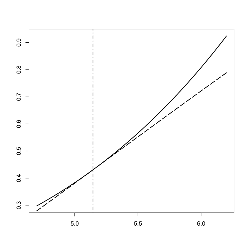
In Figure 1 we illustrate the curves x↦ci,1​ψr+(1−p)​λ​(x)x\mapsto c_{i,1}\psi_{r+(1-p)\lambda}(x) and and x↦(Rr+(1−p)​λ​hC)​(x)+di,2​φr+(1−p)​λ​(x)x\mapsto(R_{r+(1-p)\lambda}h_{C})(x)+d_{i,2}\varphi_{r+(1-p)\lambda}(x) around the optimal entry threshold x∗x^{*} under the parameter configuration α=0.05\alpha=0.05, β=0.25\beta=0.25, r=0.1r=0.1, K=C=λ=1K=C=\lambda=1, and p=0.5p=0.5. The figure suggests that the curves tangent at x∗x^{*}. This is in line with the smoothness requirement of GiG_{i}.

Figure 1. The curves x↦ci,1​ψr+(1−p)​λ​(x)x\mapsto c_{i,1}\psi_{r+(1-p)\lambda}(x) (solid black line) and x↦(Rr+(1−p)​λ​hC)​(x)+di,2​φr+(1−p)​λ​(x)x\mapsto(R_{r+(1-p)\lambda}h_{C})(x)+d_{i,2}\varphi_{r+(1-p)\lambda}(x) (dashes black line). The grey dashed line is located at x∗=5.144979x^{*}=5.144979.
Refer to caption

In Figure 2 we illustrate the effect of parameter pp on the value GiG_{i} under the parameter configuration α=0.05\alpha=0.05, β=0.25\beta=0.25, r=0.1r=0.1, and K=C=λ=1K=C=\lambda=1. The values of pp are 0.80.8, 0.60.6, 0.40.4, and 0.20.2 and the curves are colored such that the hue becomes lighter as the probability pp decreases. The figure shows that decreasing pp decreases value, this is in line with our general result.
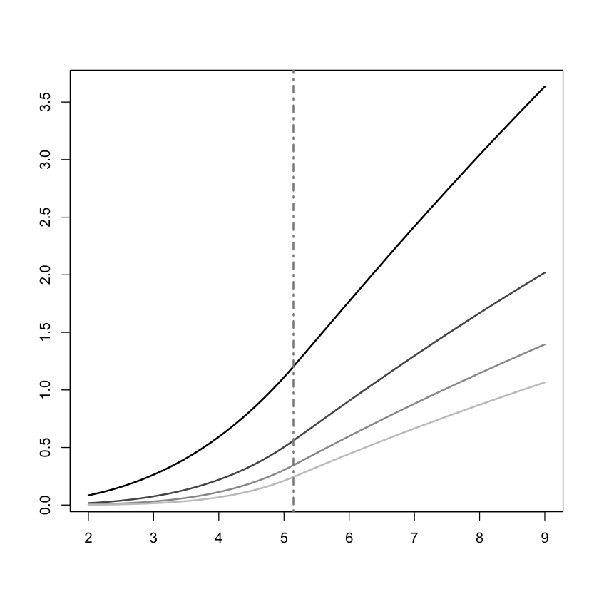
Figure 2. The value GiG_{i} for different values of pp, p=0.8,0.6,0.4,0.2p=0.8,0.6,0.4,0.2. The hue of the curve becomes lighter as the probability pp decreases. The grey dashed line marks the optimal entry threshold x∗=5.144979x^{*}=5.144979.
Refer to caption

5.2. Logistic Diffusion [7]

As a generalization of the geometric Brownian motion, we consider the diffusion XX with infinitesimal generator

𝒜=12​β2​x2​d2d​x2+α​x​(1−γ​x)​dd​x,\mathcal{A}=\frac{1}{2}\beta^{2}x^{2}\frac{d^{2}}{dx^{2}}+\alpha x(1-\gamma x)\frac{d}{dx},

with α\alpha, β\beta, and γ\gamma positive. This process exhibits mean reversion and has been applied successfully in investment theory, see [7]. We point out that when γ=0\gamma=0, this process reduces to a geometric Brownian motion.

A straightforward computation yields the functions S′S^{\prime} and m′m^{\prime}: S′​(x)=x−2​μσ2​e2​γ​μσ2​xS^{\prime}(x)=x^{-\frac{2\mu}{\sigma^{2}}}e^{\frac{2\gamma\mu}{\sigma^{2}}x} and m′​(x)=2(σ​x)2​x2​μσ2​e−2​γ​μσ2​xm^{\prime}(x)=\frac{2}{(\sigma x)^{2}}x^{\frac{2\mu}{\sigma^{2}}}e^{-\frac{2\gamma\mu}{\sigma^{2}}x} for all x∈(0,∞)x\in(0,\infty). Furthermore, it is known from the literature that for an arbitrary ρ>0\rho>0, the functions ψρ\psi_{\rho} and φρ\varphi_{\rho} reads as

ψρ​(x)\displaystyle\psi_{\rho}(x) =xb⁡(ρ)​M​(b⁡(ρ),2​b​(ρ)+2​μσ2,2​μ​γσ2​x),\displaystyle=x^{b(\rho)}M(b(\rho),2b(\rho)+\frac{2\mu}{\sigma^{2}},\frac{2\mu\gamma}{\sigma^{2}}x),
ψρ​(x)\displaystyle\psi_{\rho}(x) =xb⁡(ρ)​U​(b⁡(ρ),2​b​(ρ)+2​μσ2,2​μ​γσ2​x),\displaystyle=x^{b(\rho)}U(b(\rho),2b(\rho)+\frac{2\mu}{\sigma^{2}},\frac{2\mu\gamma}{\sigma^{2}}x),

where MM and UU are, respectively, the confluent hypergeometric functions of first and second type, see [4]. Due to the complicated nature of these functions, we resort to numerical solution of the optimal entry threshold x∗x^{*} and the value function GiG_{i}.

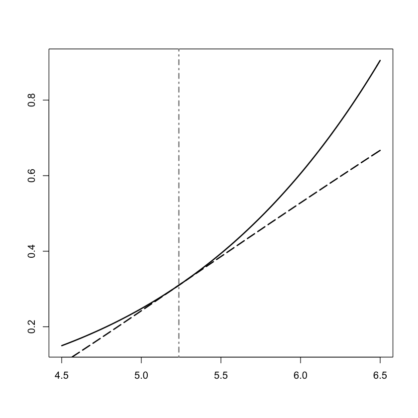
In Figure 3 we illustrate the curves x↦ci,1​ψr+(1−p)​λ​(x)x\mapsto c_{i,1}\psi_{r+(1-p)\lambda}(x) and and x↦(Rr+(1−p)​λ​hC)​(x)+di,2​φr+(1−p)​λ​(x)x\mapsto(R_{r+(1-p)\lambda}h_{C})(x)+d_{i,2}\varphi_{r+(1-p)\lambda}(x) around the optimal entry threshold x∗x^{*} under the parameter configuration α=0.05\alpha=0.05, β=0.25\beta=0.25, r=0.1r=0.1, K=C=λ=1K=C=\lambda=1, γ=0.2\gamma=0.2, and p=0.5p=0.5. The figure suggests that the curves tangent at x∗x^{*}.

Figure 3. The curves x↦ci,1​ψr+(1−p)​λ​(x)x\mapsto c_{i,1}\psi_{r+(1-p)\lambda}(x) (solid black line) and x↦(Rr+(1−p)​λ​hC)​(x)+di,2​φr+(1−p)​λ​(x)x\mapsto(R_{r+(1-p)\lambda}h_{C})(x)+d_{i,2}\varphi_{r+(1-p)\lambda}(x) (dashes black line). The grey dashed line is located at x∗=5.235711x^{*}=5.235711.
Refer to caption

In Figure 4 we illustrate the effect of parameter pp on the value GiG_{i} under the parameter configuration α=0.05\alpha=0.05, β=0.25\beta=0.25, r=0.1r=0.1, K=C=λ=1K=C=\lambda=1, and γ=0.2\gamma=0.2. The values of pp are 0.80.8, 0.60.6, 0.40.4, and 0.20.2 and the curves are colored such that the hue becomes lighter as the probability pp decreases. The figure shows that decreasing pp decreases value, this is in line with our general result.
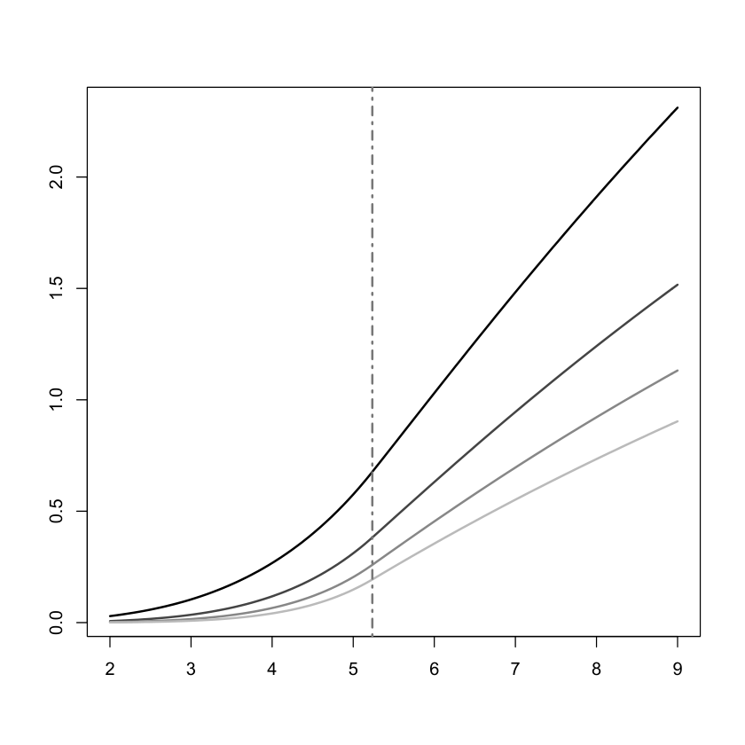
Figure 4. The value GiG_{i} for different values of pp, p=0.8,0.6,0.4,0.2p=0.8,0.6,0.4,0.2. The hue of the curve becomes lighter as the probability pp decreases. The grey dashed line marks the optimal entry threshold x∗=5.235711x^{*}=5.235711.
Refer to caption

References

  • [1] Borodin, A. and P. Salminen (2015). Handbook on Brownian Motion – Facts and Formulæ. 2nd Edition, Birkhäuser, Basel
  • [2] Bronstein, A. L. and M. Zervos (2006). Sequential entry and exit decisions with an ergodic performance criterion. Stochastics, 78/2, 99 – 121
  • [3] Chung, K. L. and J. B. Walsh (2005). Markov Processes, Brownian Motion and Time Symmetry. Springer, New York
  • [4] Dayanik, S. and I. Karatzas (2003). On the optimal stopping problem for one-dimensional diffusions. Stochastic Processes and Their Applications, 107/2, 173 – 212
  • [5] Diamond, D. W. and R. G. Rajan (2001). Liquidity Risk, Liquidity Creation, and Financial Fragility: A Theory of Banking. Journal of Political Economy, 109, 287 – 327
  • [6] Dixit, A. K. (1989). Entry and Exit Decisions under Uncertainty. Journal of Political Economy, 97, 620 – 638
  • [7] Dixit, A. K. and R. S. Pindyck (1994). Investment under Uncertainty. Princeton University Press
  • [8] Duckworth, J. K. and M. Zervos (2000). An Investment Model with Entry and Exit Decisions. Journal of Applied Probability, 37, 547 – 559.
  • [9] Lempa, J. (2012). Optimal Stopping with Information Constraint. Applied Mathematics and Optimization, 66/2, 147 – 173
  • [10] Serfozo, R. (2009). Basics of Applied Stochastic Processes. Springer, Berlin
  • [11] Wang, H. (2005). A Sequential Entry Problem with Forced Exits. Mathematics of Operations Research, 30/2, 501 – 520
  • [12] Zervos, M. (2003). A Problem of Sequential Entry and Exit Decisions Combined with Discretionary Stopping. SIAM Journal on Control and Optimization, 42/2, 397 – 421