Self-interaction in the Bopp-Podolsky electrodynamics: Spacetimes with angular defects

The formalism of BP electrodynamics starts from the Lagrangian

where $A_{i}$ is the electromagnetic field potential, $F_{ik}=\nabla_{i}A_{k}-\nabla_{k}A_{i}$ is the Maxwell tensor, $\nabla_{i}$ denotes the covariant derivative, and $j^{i}$ is the current density. The variation procedure with respect to the potentials $A_{i}$ gives the electromagnetic field equation

It is easy to see the BP Lagrangian (2) and the BP equation (3) reduce to the standard Maxwellian form when $\mu\to\infty$.

Solutions of the fourth-order equations (3) can be written as a difference between $A_{i}^{(0)}$ and $A_{i}^{(\mu)}$ (see [6]),

where the first term is a solution to the Maxwell equation, while the second one obeys the Proca equation with the same current density:

Thus, Eq. (3) splits into two second-order equations describing, correspondingly, massless and massive (with the mass $\mu$) vector fields. In this sense, the BP model has a close relationship with the Pauli-Villars regularization procedure (see, e.g., [14]) and Lee-Wick model [15] (see also the recent papers [16]).

The electromagnetic field energy-momentum tensor derived by the variation with respect to the metric from the action with the Lagrangian (2) of this model takes the form

When the potential $A_{i}$ satisfies the BP model equation (3), the energy-momentum tensor is also splitting into two parts: $T_{ik}^{BP}=T_{ik}^{(0)}-T_{ik}^{(\mu)}$, where the first one,

corresponds to the massless vector field $A_{i}^{(0)}$, and the second one,

is the energy-momentum tensor of the Proca-type massive field $A_{i}^{(\mu)}$. This field has a negative energy and therefore it can be interpreted as a phantom one.

When the particle is at rest, its current density is

where $q$ is a charge of the particle, $\delta(x)$ is the Dirac delta function, ${\bf r}_{c}$ denotes a radius-vector of a charge position, and the field potential in the framework of the BP electrodynamics [6, 9, 7] takes the form

For $\mu|\mathbf{r}-\mathbf{r}_{c}|\gg 1$ this formula turns into the well-known expression for the Coulomb electrostatic potential, but at the origin it has no singularity, $\lim\limits_{\mathbf{r}\to\mathbf{r}_{c}}A_{0}=\mu q$. The energy of the electrostatic field (9) in the BP model is also finite and expressed by the formula

Since in the BP model the expression of the point charge field potential is free from a singularity at the origin, in order to derive a formula for the self-force $f^{i}_{\rm sf}$, we could write down directly

where $F^{ik}$ is the Maxwell tensor of the electromagnetic field produced by the moving particle, and $u_{k}$ is its velocity vector, and both quantities have to be calculated at the present position of the charged particle.

However, for the static field potential (9) in the Minkowski spacetime, when $\mathbf{r}\to\mathbf{r}_{c}$ we have

It is easy to see that the strength tensor field (12) has a hedgehog-like singularity at the point of charge. Therefore, in order to calculate the force acting on the charge we should average the expression (12) over a solid angle. After this procedure we come to the predictable result: for the static charge in the Minkowski spacetime $f_{\rm sf}^{i}=0$. So, when we use the formula (11), the mentioned procedure of averaging should be always implied.

On the other hand, the expression (11) can be rewritten in the static case ($u^{i}=u^{0}\delta^{i}_{0}$) as follows

where $G^{(0)}(\mathbf{r},\mathbf{r}_{c})$ and $G^{(\mu)}(\mathbf{r},\mathbf{r}_{c})$ are the three-dimensional Green functions for Eqs. (4) and (5), respectively. Since, due to the reciprocity principle, the Green functions are symmetric with respect to the permutation of their arguments,

the formula (13) can be transformed into

where the quantity $U$ plays the role of the self-interaction potential energy. Mention that calculation of the self-interaction energy for the static point charge in the Minkowski spacetime ($u^{0}=1$) yields

and therefore $f^{i}_{\rm sf}=0$. It means that the second approach implies the averaging procedure automatically.

For the sake of simplicity, let us consider a static axially symmetric spacetime, the metric of which takes the form

Here $\rho\in[0;+\infty)$ is a radial coordinate, $\varphi\in[0;2\pi]$ is an azimuthal angle, and $R(\rho)$ is a unique unknown function, which will be defined later.

We will assume that a static charge is located at the point $(\rho_{c},\varphi_{c},z_{c})$ of this spacetime. The Green functions $G^{(0)}(\mathbf{r},\mathbf{r}_{c})$ and $G^{(\mu)}(\mathbf{r},\mathbf{r}_{c})$ obey the equations

where $\triangle$ is the Laplace operator relating to the spacetime with the metric (18):

The solutions to Eqs. (19), (20) can be represented as follows (see, e.g., [1], p. 125)

where the radial Green functions $g^{(0)}_{n\tau}$ and $g^{(\mu)}_{n\tau}$ satisfy the equations

respectively, and the prime denotes the derivative with respect to $\rho$. These functions can be written in the following form (for $g_{n\tau}^{(0)}$ we should put $\mu=0$),

where $y_{n\tau}^{1(\mu)}(\rho)$ and $y_{n\tau}^{2(\mu)}(\rho)$ are the solutions of the corresponding homogeneous equation

which are regular at $\rho=0$ and at $\rho=\infty$, respectively, and normalized by their Wronskian,

Now, to derive the formula for the self-interaction energy we can apply Eq. (16). Since $u^{0}=1$ for the metric (18), in the limit case ${\bf r}\to{\bf r}_{c}$ (i.e., $\rho\to\rho_{c}$, $\varphi\to\varphi_{c}$, $z\to z_{c}$), we obtain

Obviously, this function depends only on the radial coordinate of the charge position $\rho_{c}$.

For further progress we should fix the metric function $R(\rho)$. As an example, we consider the spacetime of a straight infinitely thin cosmic string, for which

where $b$ is a positive parameter related to a linear mass density of a string. When $b<1$ the density is positive, when $b>1$ it is negative, and in the case $b=1$ we deal with the standard Minkowski spacetime. From a spacetime geometry point of view, this parameter specifies the quantity of the spacetime angular defect.

A set of solutions to the homogeneous equation (27), regular at $\rho=0$ ($y_{n\tau}^{1(0)}$ and $y_{n\tau}^{1(\mu)}$) or at $\rho=\infty$ ($y_{n\tau}^{2(0)}$ and $y_{n\tau}^{2(\mu)}$), and satisfying the condition (28) takes the form

where ${\rm I}_{\nu}(x)$ and ${\rm K}_{\nu}(x)$ are the modified Bessel functions of the first and second kind, respectively. Substituting these expressions into (29), we obtain

In order to reduce this formula, as the first step, we apply the integral representation for the product of the Bessel functions (see [17]),

where ${\rm J}_{\nu}(x)$ is the Bessel function, with the identity

and evaluate the series:

The swapping integration and summation in (37) is possible, because if $\tau\neq 0$ the integral $\int_{0}^{\infty}dxf_{n}(x)$ and the series $\sum_{n}f_{n}(x)$, where

converge uniformly. Since the Bessel function ${\rm J}_{0}(x)$ at the origin behaves as ${\rm J}_{0}(x)\approx 1-x^{2}/4$, the integrand in the right-hand side of (37) is finite when $x\to 0$. Now we can integrate this expression over $\tau$. As a result, we obtain

where $U_{0}=\mu q^{2}/2$ is the charge field energy for the Minkowski spacetime (10), i.e., when $b=1$.

It is worth noting that in Eq. (38) we have interchanged the order of integration

where

To justify this transformation, let us consider, firstly, the case when both lower limits are nonzero. The swapping $\int_{A}^{\infty}d\tau\int_{B}^{\infty}dx=\int_{B}^{\infty}dx\int_{A}^{\infty}d\tau$ is allowed, because the integrals $\int_{A}^{\infty}d\tau F(\tau,x)$ and $\int_{B}^{\infty}dxF(\tau,x)$ converge uniformly for $x>B>0$ and $\tau>A>0$, respectively. Second, since at $x\to 0$ we have $F(\tau,x)\approx\mu^{2}\rho^{2}bx>0$, there exists a region in the vicinity of the origin (say, $x\in[0,B]$), where the function $F(\tau,x)$ is nonnegative. Due to a theorem from [18] the swapping $\int_{0}^{\infty}d\tau\int_{0}^{B}dx=\int_{0}^{B}dx\int_{0}^{\infty}d\tau$ is allowed again. At last, since the integral $\int_{0}^{\infty}dxF(\tau,x)$ has an integrable singularity at $\tau=0$, to prove the interchanging $\int_{0}^{A}d\tau\int_{0}^{\infty}dx=\int_{0}^{\infty}dx\int_{0}^{A}d\tau$ we should change a variable $\tau\to 1/\tau$. Obtained integrals converge uniformly as well.

From Eq. (38), one can see that the self-interaction potential energy depends on the dimensionless parameter $\mu\rho$ only. In order to demonstrate this dependence in the explicit form, we should consider the integral in (38) on the complex plane,

and change the path of integration. The new contour consists of two parts: first, the half-line $\mathop{\rm Im}\nolimits z=\pi/2,\ \mathop{\rm Re}\nolimits z\leq 0$, and second, the segment of the imaginary axis $\mathop{\rm Im}\nolimits z\in(0;\pi/2)$; meanwhile, the poles $z=\pi bni$ of the function $\coth z/b$ ($n$ is integer and less than $1/2b$) and the point $z=0$ should be excluded.

After some routine calculations we obtain (38) in the new, more convenient form,

This relation generalizes the corresponding formulas from [19] and [20] for the BP electrodynamics. If the angular defect parameter $b=1/(2N+1)$, where $N$ is nonnegative integer, the last term in (40) vanishes and this formula reduces to

In contrast, if $b=1/(2N)$ the last term tends to $\frac{1}{2\mu\rho}(1-\exp(-2\mu\rho))$, and the formula (40) transforms to

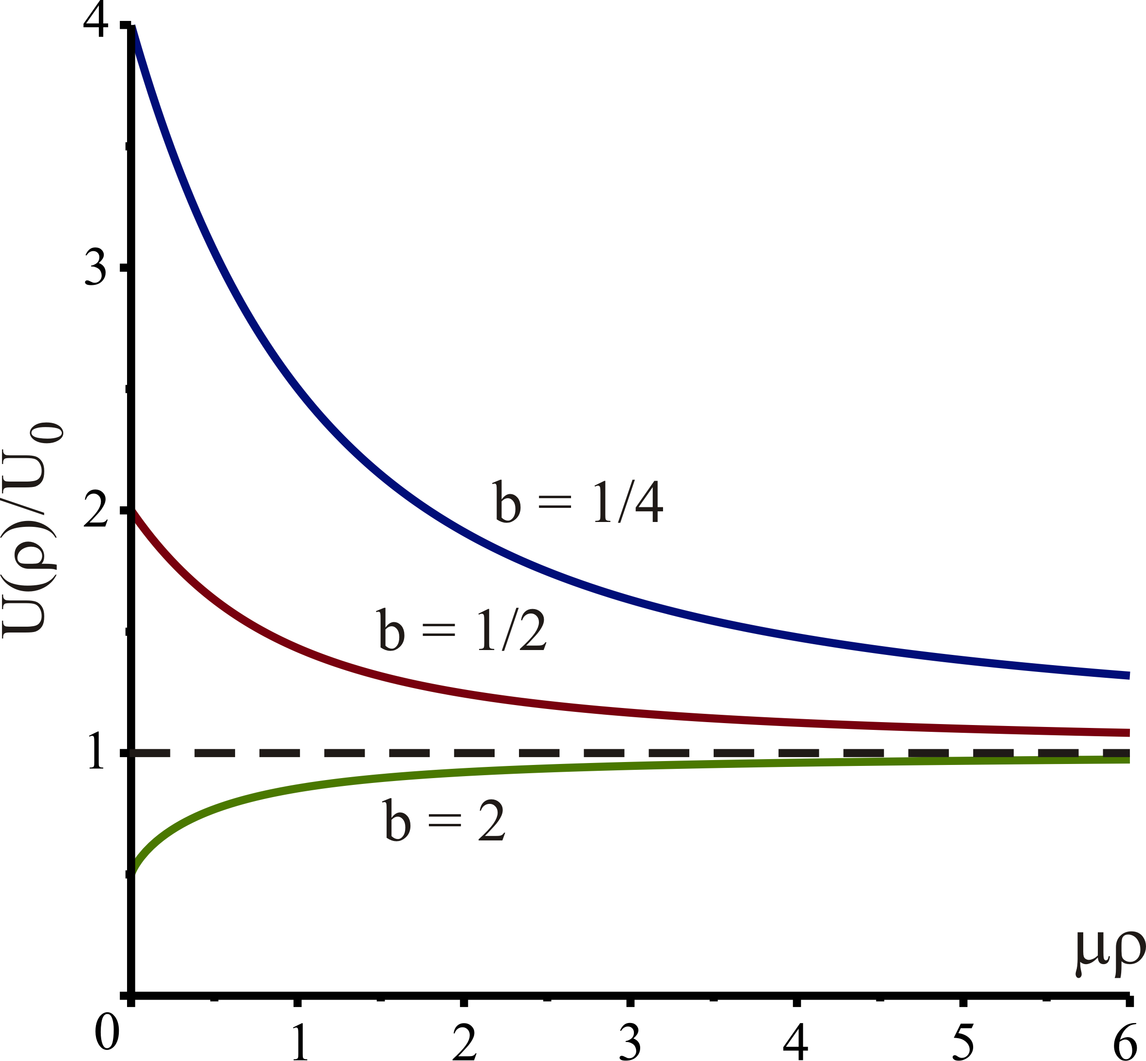
When $\rho\to\infty$ the function $U(\rho)$ obviously tends to $U_{0}$, while at the origin $U(0)=U_{0}/b$. Plots of the function $U(\rho)$ for some values of the parameter $b$ are presented in Fig. 1.

Let us consider the formula (40) in two limiting cases. First, when the angular defect (or the string mass density) is very small, i.e., for $|1-b|\ll 1$, Eq. (40) yields

Second, when $\mu\rho\gg 1$ the asymptotic behavior of $U(\rho)/U_{0}$ is determined by the expression

where

and the remainder term $L(\mu\rho,b)$ behaves as follows:

The term $P(b)/(\mu\rho)$ in the second form is a standard renormalized expression for the self-interaction potential energy [21] in the Maxwell model. In the framework of the BP electrodynamics, we derive it as the limiting case of the general formula (40) without any regularization procedure.

Analyzing the obtained function $U(\rho)$ for the self-interaction energy, we can conclude that if $b>1$, the function $U(\rho)$ is an increasing one, and the self-force attracts the charge to the cosmic string. In contrast, when $b<1$ the function $U(\rho)$ is a decreasing one, and in this case repulsion between the charge and the string occurs.

Let us proceed to the case, when the spacetime is static and it has the spherical symmetry. For the sake of simplicity, the metric of this spacetime takes the form

where $r\in[0;+\infty)$ is a radial coordinate, $\theta\in[0;\pi]$ and $\varphi\in[0;2\pi]$ are angular coordinates of the spherical system. $R(r)$ is a unique undefined metric function.

We will assume that a static charge is placed at the point ($r_{c}$, $\theta_{c}$, $\varphi_{c}$) of the spacetime. In order to derive the expression for the self-interaction potential energy we use the same scheme as it was demonstrated above. The Green functions $G^{(0)}(\mathbf{r},\mathbf{r}_{c})$ and $G^{(\mu)}(\mathbf{r},\mathbf{r}_{c})$ satisfy the equations

The Laplacian relating to the spacetime metric (47) takes the form

The solutions to Eqs. (48), (49) can be represented as follows (see, e.g., [1], p. 120):

where the radial Green functions $g^{(0)}_{n}$ and $g^{(\mu)}_{n}$ satisfy the equations

respectively, ${\rm Y}_{nm}(\theta,\varphi)$ is the spherical function, and the asterisk denotes complex conjugation. In contrast with the previous section, here the prime relates to the derivative with respect to $r$.

These functions can be written in the following form (for $g_{n}^{(0)}$ we should put $\mu=0$),

where $y_{n}^{1(\mu)}(r)$ and $y_{n}^{2(\mu)}(r)$ are the solutions of the corresponding homogeneous equation

which are regular at $r=0$ and at $r=\infty$, respectively, and normalized by their Wronskian

For the metric (47) we have $u^{0}=1$ (see (16)) and the self-interaction energy formula gives

It is easy to see this function depends only on the radial coordinate of the charge position $r_{c}$.

Let us fix again the metric function $R(r)$. As an example we consider the spacetime of a global monopole spacetime, for which

where $b$ is a positive parameter related to the scale characterizing spontaneous symmetry breaking. In the case $b=1$ we deal again with the standard Minkowski spacetime. When $b\neq 1$ this spacetime possesses the conic singularity at the origin and it is not locally flat. From this point of view, the parameter $b$ determines a defect of solid angle.

In this case, solutions to the homogeneous equation (56), regular at $r=0$ ($y_{n}^{1(0)}$ and $y_{n}^{1(\mu)}$) or at $r=\infty$ ($y_{n}^{2(0)}$ and $y_{n}^{2(\mu)}$), and obeying the condition (57) take the form

References

• [1] J. D. Jackson, Classical Electrodynamics, Wiley, 1999.
• [2] F. Rohrlich, Classical Charged Particles, World Scientific, 2007.
• [3] H. Spohn, Dynamics of Charged Particled and Their Radiation Field, Cambridge University Press, 2007.
• [4] N. R. Khusnutdinov, Phys. Usp. 48, 577 (2005);
E. Poisson, A. Pound, and I. Vega, Liv. Rev. Rel. 14, 7 (2011).
• [5] M. Born and L. Infeld, Proc. Roy. Soc. London A 144, 425 (1934).
• [6] F. Bopp, Ann. Phys. (Leipzig) 38, 345 (1940).
• [7] B. Podolsky, Phys. Rev. 62, 68 (1942).
• [8] D. Chruściński, Phys. Lett. A 240, 8 (1998);
V. Perlick, Fund. Theor. Phys. 179, 523 (2015).
• [9] A. Landé and L.H. Thomas, Phys. Rev. 60, 514 (1941).
• [10] J. Gratus, V. Perlick, and R. W. Tucker, J. Phys. A 48, 435401 (2015).
• [11] A. E. Zayats, Ann. Phys. (N.Y.) 342, 11 (2014).
• [12] J. R. Gott III, Astrophys. J. 288, 422 (1985);
W. A. Hiscock, Phys. Rev. D31, 3288 (1985);
B. Linet, Gen. Relativ. Gravit. 17, 1109 (1985).
• [13] M. Barriola and A. Vilenkin, Phys. Rev. Lett. 63, 341 (1989).
• [14] J. Kvasnica, Czech. J. Phys. B 10, 81 (1960).
• [15] T. D. Lee and G. C. Wick, Nucl. Phys. B 9, 209 (1969);
T. D. Lee and G. C. Wick, Phys. Rev. D2, 1033 (1970).
• [16] F. A. Barone, G. Flores-Hidalgo, and A. A. Nogueira, Phys. Rev. D88, 105031 (2013);
F. A. Barone and A. A. Nogueira, Eur. Phys. J. C 75, 339 (2015).
• [17] I. S. Gradshteyn and I. M. Ryzhik, Tables of Integrals, Series, and Products, Academic Press, 2007.
• [18] V. A. Zorich, Mathematical Analysis. Vol. 2, Springer, 2004.
• [19] N. R. Khusnutdinov, Classical Quantum Gravity 11, 1807 (1994);
N. R. Khusnutdinov, Theor. Math. Phys. 103, 603 (1995).
• [20] B. Linet, Ann. Inst. Henri Poincaré A 45, 249 (1986).
• [21] B. Linet, Phys. Rev. D33, 1833 (1986).
• [22] M. Abramowitz and I. Stegun, Handbook of Mathematical Functions, Dover, 1972.
• [23] E. R. Bezerra de Mello and C. Furtado, Phys. Rev. D56, 1345 (1997).
• [24] A. Vilenkin, Phys. Rev. D20, 373 (1979);
A. G. Smith and C. M. Will, Phys. Rev. D22, 1276 (1980).