Location-Aided Pilot Contamination Avoidance for Massive MIMO Systems
Abstract
Pilot contamination, defined as the interference during the channel estimation process due to reusing the same pilot sequences in neighboring cells, can severely degrade the performance of massive multiple-input multiple-output systems. In this paper, we propose a location-based approach to mitigating the pilot contamination problem for uplink multiple-input multiple-output systems. Our approach makes use of the approximate locations of mobile devices to provide good estimates of the channel statistics between the mobile devices and their corresponding base stations. Specifically, we aim at avoiding pilot contamination even when the number of base station antennas is not very large, and when multiple users from different cells, or even in the same cell, are assigned the same pilot sequence. First, we characterize a desired angular region of the target user at the serving base station based on the number of base station antennas and the location of the target user, and make the observation that in this region the interference is close to zero due to the spatial separability. Second, based on this observation, we propose pilot coordination methods for multi-user multi-cell scenarios to avoid pilot contamination. The numerical results indicate that the proposed pilot contamination avoidance schemes enhance the quality of the channel estimation and thereby improve the per-cell sum rate offered by target base stations.
Index Terms:
Interference alignment, MIMO systems, pilot contamination, location-aware communication.I Introduction
The use of very large antenna arrays at the base station (BS) is considered as a promising technology for 5G communications in order to cope with the increasing demand of wireless services [2]. Such massive multiple-input multiple-output (MIMO) systems provide numerous advantages [3, 4, 5, 6, 7, 8]: including (i) increasing the spectral efficiency by supporting a higher number of users per cell, (ii) improving energy efficiency by radiating focused beams towards users, and (iii) averaging out small scale fading resulting in the channel hardening effect. Furthermore, under the assumption of perfect channel estimation, massive MIMO provides asymptotic orthogonality between vector channels of the target and interfering users. However, performance of these systems is degraded by the pilot contamination effect, i.e., interference during uplink channel estimation due to reusing of the same pilot sequences.
Pilot sequences are a scarce resource due to the fact that the length of pilot sequences (the number of symbols) is limited by the coherence time and bandwidth of the wireless channel. As a result, the number of separable users is limited by the number of the available orthogonal pilot sequences [5, 6]. Therefore, in multi-cell massive MIMO systems, the pilot sequences must be reused, which leads to interference between identical pilot sequences from users in either neighboring cells or even the same cell; this effect is known as pilot contamination [9]. Pilot contamination is known to degrade the quality of channel state information at the BS, which in turn degrades the performance in terms of the achieved spectral efficiency, beamforming gains, and cell-edge user throughput. Since pilot contamination is an important phenomenon that degrades the performance of massive MIMO systems, we provide a detailed overview of existing works on this topic in the following subsection.
I-A Related Works
Mitigation strategies for pilot contamination have been well studied in the literature. A comprehensive survey on pilot contamination in massive MIMO systems is provided in [10]. The existing pilot decontamination methods for time division duplex (TDD) MIMO systems are broadly grouped in to two categories: pilot-based and subspace-based approaches.
In pilot-based approaches, each BS takes turns in sending pilots in a non-overlapping fashion[11, 12, 13, 14, 15]. In these works, the frame structure is modified such that the pilots are transmitted in each cell in non-overlapping time slots [12, 13], or pilots are transmitted in consecutive phases in which each BS keeps silent in one phase and repeatedly transmits in other phases [14]. Alternatively, a combination of downlink and uplink scheduled training can be used [15].
Subspace-based approaches exploit second-order statistics and utilize covariance-aided channel estimation [16, 17, 18, 7, 19, 20, 21, 22, 23, 24, 25]. Second-order statistics of desired and interfering user channels are exploited in [18, 7, 16, 17]. The works in [18, 9, 26, 16, 17] considered spatial correlated fading, while earlier works assumed uncorrelated fading. The use of non-diagonal covariance matrices enables the identification of spatially compatible users based on the spatial correlation of the covariance matrices. A closed-form expression of the non-asymptotic downlink rate exploiting the statistical second order channel covariance matrices information is provided in [24]. In [19, 20, 22], blind channel estimation with power and power-controlled hand-off is studied with singular value decomposition of the received signal matrix. The assumption that coherence time is larger than the number of BS antennas is used in [19, 20, 22] and relaxed in [21]. Blind channel estimation using eigenvalue-decomposition is described in [23].
A game-theoretic approach to tackle pilot contamination is studied in [27]. An iterative way of assigning users to pilots is proposed such that in each iteration the minimum signal-to-interference ratio is improved [28]. In [29], users in each cell are grouped based on severity of pilot contamination and a fractional pilot reuse scheme is employed. Other approaches include, among others, greater-than-one pilot reuse schemes [7, 30, 31, 32, 33, 25, 29, 34], and location-aided pilot allocation schemes [35, 36, 37]. In [35], a location-aided channel estimation method is described, wherein to mitigate the inter-cell interference where an FFT-based post-processing approach is employed after pilot-aided channel estimation. In[36], a location-aware novel pilot assignment algorithm is proposed for heterogeneous networks.The method ensures that users that are assigned to the same pilot sequence have distinguishable angle-of-arrivals (AoAs) at the macro BSs, while maintaining a large distances for the interfering users to the corresponding small BSs. The work reported in [37] proposed a location-aware pilot assignment scheme for Rician channel models and exploited the location-dependent line-of-sight (LOS) channel component during the pilot assignment procedure.
Recent insights about the impact of pilot contamination suggest that the capacity of massive MIMO systems increases without bound as the number of antennas tend to infinity, even in the presence of pilot contamination, if proper precoding/combining are employed [38]. As it is pointed out in that paper, this result does not imply that the negative effects of pilot contamination disappear, since the resulting estimation errors still degrade the performance. As our numerical results indeed show, the proposed pilot contamination avoidance scheme increases the sum rate of multicell systems.
I-B Contributions
In this work, we build on [18], which focused on a greedy pilot allocation for the asymptotic regime of infinite antennas at the BS, where pilot contamination is fully eliminated. Greedy approaches lead to performance degradation, as reported in [32], while pilot contamination does not vanish for the practical finite antenna regime. Here, we address both aspects and design explicitly for the finite-antenna regime, while targeting overall system performance by considering a joint design across multiple cells for all users in the system. More specifically, the contributions of our paper are as follows:
- •
Similar to our previous work[1], a location-aided approach is taken for pilot decontamination and we relate mean and the standard deviation of the AoA to a user location, rather than to a user’s channel.
- •
We then propose an approach with which, in the presence of location information of the users, we can quantify the effect of pilot contamination for BSs with a finite number of antennas. This result helps us predict how each user interferes with the rest of the users having identical pilot sequences when BSs are equipped with MIMO antennas, and the number of antennas is not necessarily approaching infinity. This quantification reveals that for a considerable number of antennas, there is a range of angles for which the pilot contamination is very small.
- •
Based on the above observation, we formulate pilot decontamination as an integer quadratic programming problem that we are able to solve for all the BSs as a joint optimization problem. In particular, we propose multi-cell multi-user joint optimization problems such that it takes into consideration during the pilot assignment the mutual interference seen by the target users at their respective BSs.
- •
We propose a heuristic approach for assigning users to BSs to decrease the computational complexity of the proposed joint optimization schemes. The proposed heuristic algorithm exploits both distance and AoA information of the users.
I-C Outline
The rest of the paper is structured as follows. In Section II, we introduce the system model comprising the network model, the channel model, the received pilot signal and MMSE estimator. Section III addresses the problem of pilot decontamination for BSs with (not necessarily massive) MIMO antennas. In Section IV, we present optimal user assignment and heuristic strategies for pilot contamination avoidance under various configurations, building on the theory developed in Section III. Section V demonstrates the performance of the proposed methods and we compare them with other user selection methods proposed in the literature. Finally, Section VI draws conclusions and discusses possible future directions.
Notation
Throughout the paper, vectors are written in bold lower case letters and matrices in bold upper case letters. For matrix , matrices and denote its transpose and hermitian, respectively. The -th entry of vector is denoted as . denotes stacking all the elements of in a vector. denotes a uniform distribution over the intervals defined by the set . A sequence of elements is written in short as . The positive operator is denoted as . The Kronecker product of two matrices and is denoted as . denotes the identity matrix of size and denotes the Euclidean norm. The cardinality of a set is denoted by . The sets of real and complex numbers are denoted by and , respectively; the -dimensional Euclidean and complex spaces are denoted by and , respectively.
Important angle symbols used in the paper are: represents the AoA support of user , where denotes the minimum AoA support angle and denotes the maximum AoA support angle. The mean AoA of user is denoted by . The AoA supports of the desired and interfering user after axis transformation are denoted by and respectively. The desired angular region of user is given by .
II System Model
II-A Network model
We consider a two-dimensional scenario with cells, and each cell is served by one BS equipped with antennas. We denote as the set of all cells and where the set of users in the -th cell, . The set of neighboring cells to the -th cell is denoted by . Users, equipped with a single antenna, are located uniformly within the cells. The location of user is denoted by , while the location of the BS in the -th cell is written as . We define as the set of available orthogonal pilots for allocation to users.
II-B Channel Model
The uplink channel of user from cell to BS is denoted by . We note that the channel depends only on user and BS , but the use of the additional index allows us to distinguish in which cell the users belong to. We consider the channel as the superposition of a large number of paths [18, 26, 39]:
| (1) |
where , for path-loss exponent and a known11 1 The constant depends on cell-edge signal-to-noise ratio (SNR), as specified in the numerical results. constant , is the antenna steering vector corresponding to AoA , is the path index, and is the random phase of the -th path. We restrict ourselves to uniform linear arrays with , for the antenna spacing and the signal wavelength . Under the assumption of and i.i.d. AoAs with common probability density , application of the law of large numbers (center limit theorem) gives rise to having a zero-mean Gaussian distribution with covariance matrix
| (2) | ||||
| (3) |
We further assume that corresponds to a uniform distribution with support , for some fixed , . Finally, we assume that a map exists in the BS, associating the user’s position to the support of the AoA distribution as well as the average received power (i.e., in the form of a radio map).
Remark 1.
In some scenarios, especially when the BS is elevated and seldom obstructed, propagation can be dominated by scatterers in the vicinity of the users, giving rise a limited AoA spread [26, 40, 41, 42, 43, 44], as assumed in this work. We note that the assumption of a uniform AoA distribution can be generated with the widely used ring model [39, 18, 45, 26, 46]. Such a ring model will be used for illustration and to exemplify the approach, but is not replied upon in the development of the method.
II-C Received Pilot Signal and MMSE Channel Estimator
The target user in cell sends uplink transmission to BS . Users from different cells have been assigned the same pilot sequence of length . For notational convenience, we will assume that all the users indexed with are also assigned the same pilot sequence . Later, in Section IV, we will present various ways to assign users across cells to a given pilot sequence. The received pilot signal observed at BS is written as
| (4) |
where is spatially and temporally additive white Gaussian noise (AWGN) with element-wise variance . In (4), is the desired signal channel in the cell and are the channels of interfering users.
The MMSE estimate of the desired channel by BS is given by [18, Eq. (18)]
| (5) |
where and is the covariance matrix of .
III Pilot Decontamination
In this section, we discuss pilot decontamination methods under massive and finite antenna array setting. For legibility, the extra subscripts are dropped. We consider the scenario of a given target user, say user , with channel that has arbitrary AoA distribution, but has a support . Our objective is to find an interfering user, say user in the surrounding cells and assign it the same pilot sequence as user in such a way as to minimize interference during channel estimation for user . These users have AoAs in the ranges with respect to (w.r.t.) target BS for the corresponding channels . It will turn out to be convenient to make the target BS as origin and mean AoA of user w.r.t. to BS be the new zero-degree axis. All other users are transformed according to the new coordinate system. In particular, we apply the axis transformation so that is the new zero-degrees axis. The corresponding modified AoA supports of the desired and interfering user after axis transformation are and respectively. Furthermore, we denote and The subscript denotes the user index and the superscript indicates with respect to which user the axis transformation has been applied.


III-A Massive MIMO
Note that with the term “massive MIMO”, we also refer to finite-dimensional antenna systems, similarly to most of the literature [47, 5, 48]. For a massive antenna array setting, it has been shown in [18, Theorem 1] that when the intervals are strictly non-overlapping with , i.e., , then the channel estimate tends to the interference free channel estimate , i.e., the channel estimate of the desired channel in the presence of no interfering pilot signals from other cells, obtained by setting the interference terms to zero in (5), leading to where is the received pilot signal vector at the BS under no interference from the other cell users. In fact, a sum-rate performance close to that of the interference-free channel estimation scenario is obtained for finite numbers of antennas and users. As the number of antennas goes to infinity, the pilot contamination is completely eliminated and the channel estimate of the target user reaches the interference-free scenario.
III-B Finite MIMO
Inspired by the approach in [18], we carry out the analysis that is applicable for moderate and large number of antennas . Our objective is to have a cost measure to the channel estimation quality of user when user is assigned the same pilot sequence.
III-B1 Condition for limited interference
Let us consider the desired user AoA after axis transformation is bounded by . We aim to determine for which AoAs a user causes only a small degradation to the channel estimation of user . In Appendix A, we show the interference from user with normalized steering vector is small when is small. Hence, users with steering vectors for which
| (6) | ||||
| (7) |
is small will lead to limited degradation during channel estimation of user . We have introduced
| (8) | ||||
| (9) |
Note that when and , then , as shown in [18], so that (7) also vanishes. In contrast, for finite , the shape of must be accounted for. We note that
so that users with AoA are preferred when is small, or equivalently, when , is small. The region of for which
is small is termed the desired angular region (DAR). To define the DAR, we must understand the behavior of as a function of .
III-B2 Characterization of
We characterize through its minima and maxima. It can be easily deduced that the minimum of is and is attained when the numerator becomes zero, i.e.,
| (10) |
which is equivalent to
| (11) |
where , such that and . Fig. 1 depicts the behavior of when and for various values of , where is computed numerically for all values of using (9). It can be observed that the number of zeros of the function depends on the number of antennas and it is equal to .


To ensure limited impact of user on user , should be small for all and all . Hence, we consider for at the boundaries of i.e., and , as shown in Fig. 2. We observe that both and are small for , where the values of and are detailed in Appendix B and visualized in Fig. 2.
Therefore, when the AoA support of the interfering user lies within the desired angular region () of the target user then the interference is limited. This property is exploited to devise various coordinated pilot assignment schemes in Section IV. As it is observed in Fig. 1, the range of the increases with BS antennas. The relation between , and , with is depicted in Fig. 3. Asymptotically, when , we note that and . In [18], only for the case , the AoA condition that needs to be satisfied between interfering and target users is provided, while Fig. 3 complements this for finite .
Remark 2.
For AoA distributions that are not bounded, the distribution can be bounded by truncating the support. For AoA distributions that can be described by union of multiple uniform distributions, the approach can be generalized by introducing multiple disjoint DARs.
III-B3 Approximation of cost function
The function is shown in Fig. 4 and can be approximated by a piecewise linear function (See blue dotted line in Fig. 4):

| (12) | ||||
Based on the , we define as the interference cost to the BS of user experiences from another user , which basically assigns zero cost when lies within the of user . Outside the , the cost grows linearly and saturates to at and
III-B4 Cost of pilot assignment
Based on the notion of the DAR and the function , we can finally determine a cost to user when user is assigned the same pilot. In particular, for the interfering user with , we can introduce
The interference cost is used in devising coordinated pilot assignment schemes described in Section IV.
IV Coordinated Pilot Assignment Schemes
In this section, we describe four different user assignment strategies for pilot decontamination under various configurations based on the theory developed in Section III.
IV-A Multi-User Multi-Cell Optimization
For this scenario, the goal is to reuse the pilots among the users in the best possible way such that each user has been allocated a pilot. Let us collect the users from all the cells in a set , where denotes the set of all cells and the set of users in the -th cell, . Recall that is the set of all available orthogonal pilot sequences. Let us introduce the variable , with , if -th user is activated on -th pilot and 0 otherwise. The one-shot joint optimization for user assignment for multi-user and multi-cell scenario can be written as a binary integer program (BIP):
| minimize | (13a) | |||
| (13b) | ||||
| (13c) | ||||
where
| (14) |
We note the following: (13a) gives preference to users who lie within the desired angular region of the target user; (13b) states each user must be active at least on one pilot; and (13c) imposes the binary integer requirements on the optimization variables. For each pilot, the optimization (13), looks for users in each cell with users in every cell and then chooses a set of users such that when assigned the same pilot to them, they will have minimum possible interference at their respective BSs.
The user assignment is performed based on the location for a target user, say , accounting for the following cases:
- (C1)
-
The support of interfering signals AoA lies completely inside the of the target user;
- (C2)
-
The support of interfering signal AoA lies partially inside the of the target user; and
- (C3)
-
The support of interfering signal AoA lies completely outside with the of the target user.
The above optimization problem is always feasible. The problem (13) gives preference to users that satisfy the case (C1), in which case the objective is zero. It might be possible that the user locations are such that (C1) cannot be satisfied. This is tackled in (13), as it implicitly considers the cases (C2) and (C3) in the formulation. For example, when does not lie within then the objective function becomes positive. Therefore, to minimize the objective, the interfering users are selected in such a way that the maximal overlap with the desired support of the target user is obtained.
The optimization (13) can be written as an integer quadratic constraint optimization problem (IQCP) as
| minimize | (15a) | |||
| (15b) | ||||
| (15c) | ||||
where , is a block diagonal matrix where is the utility matrix with entries
| (16) |
where is given in (14).
Remark 3.
The optimization problem (13) is formulated as an IQCP and it can be easily shown to be NP-hard. More specifically, quadratic problems (QPs) are known to be NP (see for example, [49]) and only the convex QP admits a polynomial time solution [50]. The standard QP problem where the constraints are linear, is NP-hard if matrix is indefinite [51]. In our case, the structure of matrix is non-symmetric, since in general is not necessarily equal to , and hence it is indefinite. Also, in our case, the Boolean constraints are nonconvex, since the IQCP can be written as a quadratic constrained quadratic programming (QCQP) in which .
It should be also emphasized that the above optimization problem is dependent on the number of antennas at each BS via (see (14)). Furthermore, the optimization relies on the fact that BSs acquire location information of users, which in turn incurs an overhead. Our assumption is that inter-BS communication using, for example the X2 interface in Long Term Evolution (LTE) systems, on the time scale of 100 ms would make such overhead for the inter-BS communication tolerable in a real system.
IV-B Multi-User Multi-Cell Optimization with QoS Guarantees
For the sake of establishing QoS guarantees, we may want to exclude the possibility of assigning users from the same cell as that of the target user to the same pilot. This is achieved by changing (15b) to a constraint such that only one user from each cell is assigned per pilot; this is enforced in the optimization problem via (17b). Note that if no user exists in a cell for a certain pilot, then for constraint (17b) to be valid, without loss of generality, the constraint for that cell at a certain pilot is removed. Therefore, the IQCP formulation for multi-user and multi-cell optimization with QoS guarantees is written as
| minimize | (17a) | |||
| (17b) | ||||
| (17c) | ||||
IV-C Multi-User Single-Cell Optimization
In this scenario, our objective is to find for each user in a target cell one user from the neighboring cells and assign them the same pilot sequence. For this scenario, the mutual interference of the users at the respective BSs is ignored and only the interference of the users observed at the target cell are required to be satisfied. This scenario finds applications to cases where priority is required to be given to a certain cell (for example, in case there is a special event that requires wireless communications to be robust) and in dense urban areas where it is computationally very expensive to include all the cells in the network and inevitably to run such a large-scale optimization in real time.
The set of users for this scenario are the users from the target cell and its neighboring cells. Let the set of users given by ), where is the set of cells surrounding cell The modified optimization is then written as
| minimize | (18a) | |||
| (18b) | ||||
| (18c) | ||||
where is an block diagonal matrix where is the dimension utility matrix with entries
| (19) |
IV-D Smart Pilot Assignment[28]
In this subsection, a modified smart pilot assignment of [28] for user assignment is described. The uplink signal-to-interference ratio (SINR) of -th user at -th BS is computed based on large scale fading coefficient as
which is assumed to be known, e.g., based on the distances, or from a radio map. The algorithm from [28] considers a target cell to be optimized, in the presence of already allocated pilot sequences in surrounding cells. Starting from a random allocation in the target cell, the algorithm identifies the user with minimum uplink SINR in the target cell and then tries to improve its SINR by switching pilots with another user in the target cell. This process is repeated until convergence. As this procedure is not guaranteed to converge when multiple cells are to be optimized simultaneously, we propose a modification, given in Algorithm 1.
- 1.
Initialize by randomly assigning users to pilots such that every user in each cell is assigned to one pilot.
- 2.
Sort all the users according to their uplink SINR .
- 3.
Take the user with the worst overall uplink SINR (say user in cell )
- (a)
find another user in cell with best SINR to possibly switch with, say
- (b)
if after switching
- i.
the smallest SINR is not increased, then try to find another user in cell and go to step (b). If there are no other users available in cell , STOP
- ii.
the smallest SINR is increased, do the switch and go to step 2
- i.
- (a)
IV-E Heuristic Algorithm
In this subsection, a heuristic algorithm is proposed to decrease the computational complexity of the proposed joint optimization schemes. The proposed heuristic algorithm exploits not only distance information but also AoA information. So, the algorithm assign users to pilots based on the cost (14). Recall is the cost associated if -th user and -th user are assigned to a pilot. The heuristic algorithm is similar in structure to Algorithm 1. The main difference is instead of uplink SINR, the cost is used for user assignment. The proposed heuristic algorithm is detailed in Algorithm 2. To improve the performance of the heuristic algorithm, once could use the initial user assignment obtained from Algorithm 1.
- 1.
Initialize by randomly assigning users to pilots such that every user in each cell is assigned to one pilot.
- 2.
Sort all the users according to their cost functions. Note that the cost function captures both distance and AoA information.
- 3.
Take the user with the highest overall cost (say user in cell )
- (a)
find another user in cell with lowest cost to possibly switch with, say
- (b)
if after switching
- i.
the highest cost is not decreased, then try to find another user in cell and go to step (b). If there are no other users available in cell , STOP
- ii.
the highest cost is reduced, do the switch and go to step 2
- i.
- (a)
V Numerical Results
In this section, we present numerical results to evaluate the proposed schemes described in Section IV.
V-A Simulation Scenario
| Parameter | Value |
|---|---|
| 2.5 | |
| 0.1 m | |
| 0.001 | |
| Parameter | Value |
|---|---|
| 1000 m | |
| 20 dB | |
| 50 | |
| 1W |
We consider hexagonal shaped cells and simulations are performed with a multi-cell system scenario. The simulation parameters used to obtain the numerical results are given in Table I. For a cell radius , we set to
| (20) |
where is the cell-edge SNR in dB and is the receiver noise power variance.We keep these parameters fixed for the simulations unless otherwise specified. To generate the AoA distributions, we consider a model where propagation is dominated by a ring of scatterers around the user [26, 40, 41, 42, 43, 44]. As an approximation, we consider a disk of radius comprising many scatterers around the user in cell . This radius can be different for each user depending on the environment. In that case, corresponds to a distribution with support , for some fixed , . We can calculate , , where
| (21) | ||||
| (22) |
As mentioned previously, we assume that a map exists in the base station, connecting the user’s position to the support of the AoA distribution as well as the average received power (i.e., in the form of a radio map). From those maps, it is then possible to compute , needed to compute in (5).
Remark 4.
We consider a non-LOS scenario with scattering paths. However, there might be cases where the scatterers are strong, causing large angular spreads, or cases where the location of users is not accurately known (i.e., the location estimates have uncertainty). These aspects can be incorporated into the system by allowing a larger radius , which translates to a larger range of angles. More complex AoA distributions can also be used by means of multiple scattering rings.
V-B Performance Metrics
Three different performance metrics are considered to evaluate the proposed schemes with existing approaches.
- •
Normalized mean squared error of channel estimation (NMSE) of uplink channel estimate of user at the -th BS in -th cell is denoted by and is written as
(23) where and are the desired and estimated channels of user at the -th BS in -th cell and the expectation is over many channel realizations.
- •
Cumulative distribution function of channel estimation errors: Let us define the NMSE errors in dB as ), , of the estimated channels with and without interfering users respectively, is the corresponding interference-free channel estimate. We further denote . The channel estimation errors from all cells for each pilot is collected in a set . The cumulative distribution function (CDF) is calculated on for every pilot based on several channel realizations.

Fig. 5: Comparison of channel estimation error versus BS antennas for different AoA of single interfering user. The target user is placed in m and the interfering user is placed in m from the target BS. The results are averaged over 1000 Monte-Carlo channel realizations. - •
Downlink per-cell sum rate: Assuming maximum ratio transmission, and the availability of perfect CSI at the user terminal, an upper bound on the downlink SINR of -th user at -th BS can be computed as
where . The factor in the numerator corresponds to received power, and the first and second terms in the denominator capture the intra and inter cell interference. The achievable downlink rate for the -th user in -th BS is then can be calculated as , and the sum rate of all users in a cell is obtained . Finally the per-cell downlink sum rate is given by .

(a) 
(b) Fig. 6: Performance comparison of a greedy vs joint optimization for a two cell scenario. Inset (a) two cell scenario with two users each, users are marked with a plus sign and BS with pentagons, and (b) channel estimation error as a function of the number of BS for the users in cell 1 with greedy and joint optimization schemes.
V-C Results and Discussion
V-C1 Impact of Different AoA Supports of an Interfering User
In Fig. 5, we show the impact of different ranges of AoA support of a single interfering user w.r.t. to of the target user. Note that all the angles are after the axis transformation performed w.r.t. to the target user. We can calculate , and for , it is obtained as We varied such that some are within and some are outside this range. When lies within then the interference is low, and the channel estimation converges fast to the interference-free scenario; with BS antennas the channel estimation performance is similar to that of the interference-free scenario. On the other hand, when is outside the , it can be observed that more BS antennas are needed to converge to the interference-free scenario. For example, when , then more than 50 BS antennas are required.
V-C2 Two Cell Scenario: Single Cell Optimization
We now look into the pilot allocation in a single cell, given known allocations in other cells. In particular, we consider a two-cell scenario with two users in each cell, is set to 50 m for each user, and (see Fig. 6 (a)), where the users in cell 2 have already been allocated pilots and we aim to reuse these pilots for the users in cell 1. We compare the proposed joint optimization scheme (18) with greedy sequential user assignment [1, 18]. For this scenario, both the users from cell 2 fall within the desired angular region of user 1 in cell 1. However, for user 2 of cell 1, only user 1 of cell 2 is permissible. In the greedy sequential scheme, user 1 of cell 1 is assigned the same pilot as user 1 of cell 2, since it provided the largest angular separation among the users in cell 2. Then user 2 of cell 1 has no choice but to be assigned the same pilot as user 2 in cell 2. In contrast, the joint optimization considers compatibility of both users of cell 1. Therefore, it matches user 1 of cell 1 with user 2 of cell 2 and user 2 of cell 1 with user 1 of cell 2. The channel estimation error performance for both schemes for the users in target cell (i.e., cell 1) is shown in Fig. 6 (b). As expected, the performance of pilot 2 with greedy assignment suffers as user 2 of cell 1 is not compatible with user 2 of cell 2.
V-C3 Two Cell Scenario: Multi-Cell Optimization
We now extend the discussion for the scenario above to multi-user multi-cell optimization (17). Now we can optimize the performance of both users in both cells. Therefore, the joint optimization during user assignment considers not only reducing the interference seen by the target user but also how the target user is contributing interference to users in the neighboring cells. So, users in different cells are assigned the same pilot if the AoA support of a user in one cell lies within the desired angular region of another user in another cell and vice-versa. Consequently, the channel estimation performance of the target users at their respective BS is improved. This is seen in Fig. 7, where the performance of each user in each cell approaches the interference-free condition.

When we increase the number of users per cell to 5 and set , and compare the joint assignment from Section IV-B with the smart pilot algorithm [28] described in Section IV-D, and the proposed heuristic from Section IV-E, we obtain the results in Fig. 8. We have fixed the users’ locations and the ring sizes (varying between 50 m and 100 m among users), and vary the channel and noise realizations to obtain a CDF of the channel estimation errors. This implies that the pilot assignments for each algorithms are fixed. It can be observed that all the medthods have similar performance when BS antennas. However, it was observed for when the proposed heuristic performs similar to that of joint optimization scheme, while the smart pilot scheme leads to worse performance for one of the pilots.

V-C4 Seven Cell Scenario: Multi-Cell Optimization
In this section, we will evaluate the CDF of the channel estimation errors and the sum-rate for a seven-cell scenario, with with 5 users per cell and a pilot length of . Fig. 9 shows that according to the joint optimization method, there are two bad pilots (i.e., a combination of users for which interference is unavoidably high). For dB, the heuristic outperforms the smart pilot allocation, which has two bad pilots, compared to one for the heuristic. When the number of cells is increased, it becomes even more difficult to reduce the pilot contamination for all the desired users in each cell per each pilot. The joint optimization and heuristic approaches offer relatively better performance to smart pilot scheme.

In Fig. 10, the per-cell downlink sum rate () with increase in number of BS antennas is depicted for 7-cell scenario with 5 users per cell. Furthermore, we also consider a random user assignment scheme, where in users are randomly assigned to pilots in each cell. For the random scheme, the average over the best sum rate over 1000 random pilot assignments is considered. Also, we depict the sum rate offered in the case of interference free scenario. We can clearly observe that as the number of antennas is increased the per-cell downlink sum rate is also increased. The joint optimization scheme offers better sum rate compared to the other schemes. This is due to the fact that it can better handle to avoid pilot contamination by choosing optimal user allocation. For BS antennas the joint optimization scheme gives around 11% more rate in comparison to random user assignment scheme. Furthermore, as increases the gap decreases between the sum rate offered by joint optimization scheme and the interference free scenario.
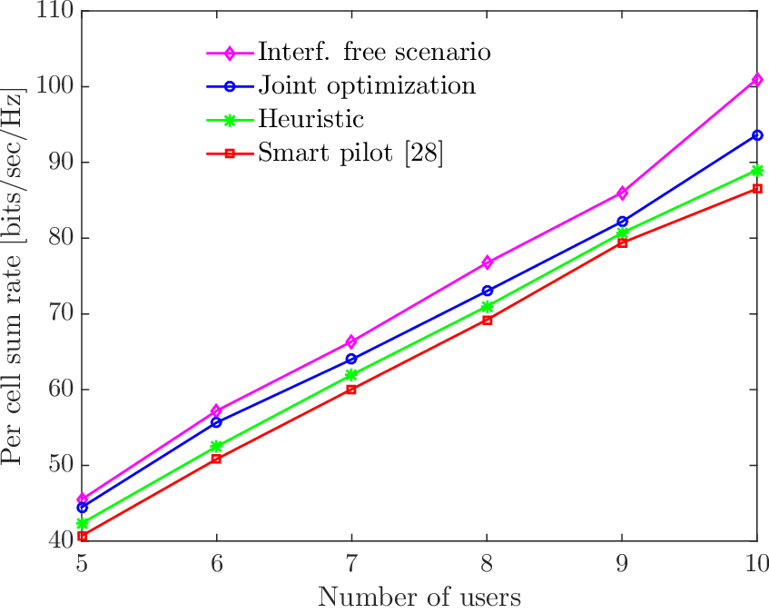
The offered sum rate by various schemes with increasing number of users per cell is shown in Fig. 11. The downlink sum rate increases with increase in number of users for all the schemes, with a widening gap between the joint optimization and the two competing methods.

VI Conclusions and Future Directions
In this paper, we characterized the effect of interference for MIMO BSs with a large, but finite, number of antennas, harnessing user location information. Building on this characterization, we formulated several pilot assignment problems as integer quadratic constraint optimization problem. These problems are solved centrally, provided that all the information about all users is shared among all BSs. To reduce the computational complexity of these joint optimization problems, we further proposed heuristic algorithm which assigns users to pilots based on both distance and angle of arrival information of the users. We show proposed pilot assignment strategies offer improved channel estimation performance as well as enhanced downlink sum rate even when the number of antennas is finite. However, low-complexity greedy methods suffer from a severe performance penalty compared to joint optimization.
Part of our ongoing research focuses on developing distributed implementations based on local information. Distributed implementations for pilot contamination avoidance under a game theoretic framework have been proposed using coalition games [52] and non-cooperative games [27]. However, none of the aforementioned approaches exploits the location information that BSs can obtain and considered in this work.
Appendix A Channel estimation under finite MIMO
The channel estimate of the desired user can be written using (4) and (5), with
as
where and the last terms constitutes the interference. We approximate by a low-rank version, i.e., , in which is an matrix. In general, for finite , is full rank, but for a sufficiently large number of antennas, , provided the AoA support of is finite [18], so low-rank approximation of exists. Then, has a rank approximation:
in which is decomposed into two orthogonal spaces. Note that may be different from .
We can now express , where is a unitary matrix spanning the orthogonal complement of . Then
The interference from user is thus determined by
Since , responses and for which indicate that causes more interference. Since , it can be used as a measure of interference. Hence, interfering users for which the steering vectors are such that is small are preferred over users for which is large, to limit the impact of interference during channel estimation for user .
Appendix B Selection of and
We denote and as the sets of zeros of functions and , respectively. The values of and are obtained by solving the following expressions using (11)
| (24) | ||||
| (25) |
We further define and .
Acknowledgment
We would like to thank Haifan Yin and David Gesbert for fruitful discussions. The authors would like to thank GUROBI for the free academic license to use their numerical optimization software.
References
- [1] L. S. Muppirisetty, H. Wymeersch, J. Karout, and G. Fodor, “Location-aided pilot contamination elimination for massive MIMO systems,” in Proc. IEEE Global Communications Conference, Dec 2015.
- [2] F. Boccardi, R. W. Heath, A. Lozano, T. L. Marzetta, and P. Popovski, “Five disruptive technology directions for 5G,” IEEE Communications Magazine, vol. 52, no. 2, pp. 74–80, Feb 2014.
- [3] Y.-G. Lim, C.-B. Chae, and G. Caire, “Performance analysis of massive MIMO for cell-boundary users,” IEEE Transactions on Wireless Communications, vol. 14, no. 12, pp. 6827–6842, Dec 2015.
- [4] E. G. Larsson, O. Edfors, F. Tufvesson, and T. L. Marzetta, “Massive MIMO for next generation wireless systems,” IEEE Communications Magazine, vol. 52, no. 2, pp. 186–195, Feb 2014.
- [5] F. Rusek, D. Persson, B. K. Lau, E. G. Larsson, T. L. Marzetta, O. Edfors, and F. Tufvesson, “Scaling up MIMO: Opportunities and challenges with very large arrays,” IEEE Signal Processing Magazine, vol. 30, no. 1, pp. 40–60, Jan 2013.
- [6] E. Bjornson, E. G. Larsson, and M. Debbah, “Optimizing multi-cell massive MIMO for spectral efficiency: How many users should be scheduled?” in Proc. IEEE Global Conference on Signal and Information Processing, Dec 2014, pp. 612–616.
- [7] T. L. Marzetta, “Noncooperative cellular wireless with unlimited numbers of base station antennas,” IEEE Transactions on Wireless Communications, vol. 9, no. 11, pp. 3590–3600, Nov 2010.
- [8] N. Rajatheva, S. Suyama, W. Zirwas, L. Thiele, G. Fodor, A. Tolli, E. D. Carvalho, and J. H. Sorensen, 5G Mobile and Wireless Communications Technology, A. Osseiran, J. F. Monserrat, and P. Marsch, Eds. Cambrdige University Press, 2016, no. ISBN 9781107130098.
- [9] J. Hoydis, S. Ten Brink, and M. Debbah, “Massive MIMO in the UL/DL of cellular networks: How many antennas do we need?” IEEE Journal on Selected Areas in Communications, vol. 31, no. 2, pp. 160–171, 2013.
- [10] O. Elijah, C. Y. Leow, T. A. Rahman, S. Nunoo, and S. Z. Iliya, “A comprehensive survey of pilot contamination in massive MIMO-5G system,” IEEE Communications Surveys &Tutorials, vol. 18, no. 2, pp. 905–923, 2016.
- [11] F. Fernandes, A. Ashikhmin, and T. L. Marzetta, “Inter-cell interference in noncooperative TDD large scale antenna systems,” IEEE Journal on Selected Areas in Communications, vol. 31, no. 2, pp. 192–201, 2013.
- [12] K. Appaiah, A. Ashikhmin, and T. L. Marzetta, “Pilot contamination reduction in multi-user TDD systems,” in Proc. IEEE International Conference on Communications, May 2010.
- [13] W. A. W. M. Mahyiddin, P. A. Martin, and P. J. Smith, “Pilot contamination reduction using time-shifted pilots in finite massive MIMO systems,” in Proc. IEEE Vehicular Technology Conference (Fall), Sep 2014.
- [14] T. X. Vu, T. A. Vu, and T. Q. S. Quek, “Successive pilot contamination elimination in multiantenna multicell networks,” IEEE Wireless Communications Letters, vol. 3, no. 6, pp. 617–620, Dec 2014.
- [15] J. Zhang, B. Zhang, S. Chen, X. Mu, M. El-Hajjar, and L. Hanzo, “Pilot Contamination Elimination for Large-Scale Multiple-Antenna Aided OFDM Systems,” IEEE Journal of Selected Topics in Signal Processing, vol. 8, no. 5, pp. 759–772, Oct 2014.
- [16] H. Yin, D. Gesbert, M. C. Filippou, and Y. Liu, “Decontaminating pilots in massive MIMO systems,” in IEEE International Conference on Communications (ICC), 2013, pp. 3170–3175.
- [17] M. Filippou, D. Gesbert, and H. Yin, “Decontaminating pilots in cognitive massive MIMO networks,” in International Symposium on Wireless Communication Systems (ISWCS), 2012, pp. 816–820.
- [18] H. Yin, D. Gesbert, M. Filippou, and Y. Liu, “A coordinated approach to channel estimation in large-scale multiple-antenna systems,” IEEE Journal on Selected Areas in Communications, vol. 31, no. 2, pp. 264–273, Feb 2013.
- [19] R. R. Mueller, M. Vehkaperae, and L. Cottatellucci, “Blind pilot decontamination,” in 17th International ITG Workshop on Smart Antennas, Mar 2013, pp. 1–6.
- [20] R. R. Muller, M. Vehkapera, and L. Cottatellucci, “Analysis of blind pilot decontamination,” in Asilomar Conference on Signals Systems and Computers, 2013, pp. 1016–1020.
- [21] R. R. Müller, L. Cottatellucci, and M. Vehkaperä, “Blind pilot decontamination,” IEEE Journal of Selected Topics in Signal Processing, vol. 8, no. 5, pp. 773–786, 2014.
- [22] L. Cottatellucci, R. R. Muller, and M. Vehkapera, “Analysis of pilot decontamination based on power control,” in 77th Vehicular Technology Conference (VTC Spring), 2013, pp. 1–5.
- [23] H. Q. Ngo and E. G. Larsson, “EVD-based channel estimation in multicell multiuser MIMO systems with very large antenna arrays,” in Proc. IEEE International Conference on Acoustics, Speech and Signal Processing, Mar 2012, pp. 3249–3252.
- [24] M. Li, S. Jin, and X. Gao, “Spatial orthogonality-based pilot reuse for multi-cell massive MIMO transmission,” in Wireless Communications & Signal Processing (WCSP), 2013 International Conference on, 2013, pp. 1–6.
- [25] L. You, X. Gao, X.-G. Xia, N. Ma, and Y. Peng, “Pilot reuse for massive MIMO transmission over spatially correlated Rayleigh fading channels,” IEEE Transactions on Wireless Communications, vol. 14, no. 6, pp. 3352–3366, 2015.
- [26] A. Adhikary, J. Nam, J.-Y. Ahn, and G. Caire, “Joint spatial division and multiplexing: The large-scale array regime,” IEEE Transactions on Information Theory, vol. 59, no. 10, pp. 6441–6463, Oct 2013.
- [27] H. Ahmadi, A. Farhang, N. Marchetti, and A. MacKenzie, “A game theoretic approach for pilot contamination avoidance in massive MIMO,” IEEE Wireless Communications Letters, vol. 5, no. 1, pp. 12–15, Feb 2016.
- [28] X. Zhu, Z. Wang, L. Dai, and C. Qian, “Smart pilot assignment for massive mimo,” IEEE Communications Letters, vol. 19, no. 9, pp. 1644–1647, Sep 2015.
- [29] D. Zhang, H. Wand, and Y. Fu, “Uplink sum rate analysis with flexible pilot reuse,” in 8th International Conference on Wireless Communications and Signal Processing (WCSP), Yangzhou, China, October 2016.
- [30] H. Yang and T. L. Marzetta, “Total energy efficiency of cellular large scale antenna system multiple access mobile networks,” in IEEE Online Conference on Green Communications (GreenCom), 2013, pp. 27–32.
- [31] Y. Li, Y.-H. Nam, B. L. Ng, and J. Zhang, “A non-asymptotic throughput for massive MIMO cellular uplink with pilot reuse,” in IEEE Global Communications Conference (GLOBECOM), 2012, pp. 4500–4504.
- [32] V. Saxena, G. Fodor, and E. Karipidis, “Mitigating pilot contamination by pilot reuse and power control schemes for massive MIMO systems,” in Proc. IEEE Vehicular Technology Conference Spring, May 2015.
- [33] M. Li, S. Jin, and X. Gao, “Spatial orthogonality-based pilot reuse for multi-cell massive MIMO transmission,” in International Conference on Wireless Communications and Signal Porcessing (WCSP), Hangzhou, China, 24-26 October 2013.
- [34] J. Li, L. Xiao, X. Xu, and S. Zhou, “Sectorization based pilot reuse for improving net spectral efficiency in the multicell massive MIMO system,” Science China Information Sciences, vol. 59(2):022307, February 2016.
- [35] Z. Wang, C. Qian, L. Dai, J. Chen, C. Sun, and S. Chen, “Location-based channel estimation and pilot assignment for massive MIMO systems,” in IEEE International Conference on Communication Workshop (ICCW), June 2015, pp. 1264–1268.
- [36] P. Zhao, Z. Wang, C. Qian, L. Dai, and S. Chen, “Location-aware pilot assignment for massive MIMO systems in heterogeneous networks,” IEEE Transactions on Vehicular Technology, vol. 65, no. 8, pp. 6815–6821, Aug 2016.
- [37] N. Akbar, S. Yan, N. Yang, and J. Yuan, “Mitigating pilot contamination through location-aware pilot assignment in massive MIMO networks,” in IEEE Globecom Workshops (GC Wkshps), Dec 2016, pp. 1–6.
- [38] E. Björnson, J. Hoydis, and L. Sanguinetti, “Massive mimo has unlimited capacity,” arXiv preprint arXiv:1705.00538, 2017.
- [39] J.-A. Tsai, R. Buehrer, and B. Woerner, “The impact of AOA energy distribution on the spatial fading correlation of linear antenna array,” in 55th IEEE Vehicular Technology Conference (Spring), vol. 2, 2002, pp. 933–937.
- [40] D. S. Shiu, G. Foschini, M. J. Gans, and J. M. Kahn, “Fading correlation and its effect on the capacity of multielement antenna systems,” IEEE Transactions on Communications, vol. 48, no. 3, pp. 502–513, March 2000.
- [41] A. Abdi and M. Kaveh, “A space-time correlation model for multielement antenna systems in mobile fading channels,” IEEE Journal on Selected Areas in Communications, vol. 20, no. 3, pp. 550–560, April 2002.
- [42] C. Oestges, B. Clerckx, D. Vanhoenacker-Janvier, and A. J. Paulraj, “Impact of diagonal correlations on MIMO capacity: Application to geometrical scattering models,” in Proc. 58th IEEE Vehicle Technology Conference, vol. 1, October 2003, pp. 394–398.
- [43] C. Oestges and A. J. Paulraj, “Beneficial impact of channel correlations on MIMO capacity,” IEEE Electronics Letters, vol. 40, no. 10, May 2004.
- [44] M. Zhang, P. J. Smith, and M. Shafi, “An extended one-ring MIMO channel model,” IEEE Transactions on Wireless Communications, vol. 6, no. 8, pp. 2759–2764, August 2007.
- [45] Z. Gao, L. Dai, Z. Wang, and S. Chen, “Spatially common sparsity based adaptive channel estimation and feedback for FDD massive MIMO,” IEEE Transactions on Signal Processing, vol. 63, no. 23, pp. 6169–6183, Dec 2015.
- [46] J. Fang, X. Li, H. Li, and F. Gao, “Low-rank covariance-assisted downlink training and channel estimation for FDD massive MIMO systems,” IEEE Transactions on Wireless Communications, vol. 16, no. 3, pp. 1935–1947, March 2017.
- [47] H. Huh, G. Caire, H. C. Papadopoulos, and S. A. Ramprashad, “Achieving "Massive MIMO" spectral efficiency with a not-so-large number of antennas,” IEEE Transactions on Wireless Communications, vol. 11, no. 9, pp. 3226–3239, September 2012.
- [48] H. Q. Ngo, E. G. Larsson, and T. L. Marzetta, “Massive MU-MIMO downlink TDD systems with linear precoding and downlink pilots,” in 51st Annual Allerton Conference, Allerton House, UIUC, Illinois, USA, October 2-3 2013, pp. 293–298.
- [49] S. A. Vavasis, “Quadratic programming is in NP,” Information Processing Letters, vol. 36, no. 2, pp. 73–77, 1990.
- [50] M. Kozlov, S. Tarasov, and L. Khachiyan, “The polynomial solvability of convex quadratic programming,” USSR Computational Mathematics and Mathematical Physics, vol. 20, no. 5, pp. 223–228, 1980.
- [51] S. Sahni, “Computationally related problems,” SIAM Journal on Computing, vol. 3, no. 4, pp. 262–279, 1974.
- [52] R. Mochaourab, E. Björnson, and M. Bengtsson, “Adaptive pilot clustering in heterogeneous massive MIMO networks,” IEEE Transactions on Wireless Communications, vol. 15, no. 8, pp. 5555–5568, Aug 2016.