Scale genesis and gravitational wave in a classically scale invariant extension of the standard model

One of the problems of the standard model (SM) is that it cannot explain the origin of the electroweak (EW) scale. Obviously, if we start with a theory which contains a scale from the beginning, we have no chance to explain its origin. We recall that the Higgs mass term is the only term that breaks scale invariance at the classical level in the SM. So, a central question is: What is the origin of the Higgs mass term? Recently, a number of studies on a scale invariant extension of the SM have been performed, where two ideas have been considered. The one [1, 2, 3, 4, 5, 6, 7, 8, 9, 10, 11, 12, 14, 15, 16, 17, 18, 13, 19, 20, 21, 22, 23, 24, 25, 26, 27, 28, 29, 30, 31, 32, 33, 34, 35, 36, 37, 38, 39, 40, 41, 42, 43] relies on the Coleman-Weinberg (CW) potential [44], and the other one is based on non-perturbative effects: Dynamical chiral symmetry breaking [45, 46] is applied in [47, 48, 49, 50, 51, 52, 53, 54, 55, 56, 57, 58, 59] and gauge-invariant scalar-bilinear condensation [60, 61, 62] is used in [63, 64].

In the case that a scale is dynamically created, there will be a corresponding scale phase transition. Chiral phase transition is a scale phase transition in this context. If a scale phase transition is strongly first-order, the Universe undergoes a strong phase transition at a certain high temperature, thereby producing gravitational wave (GW) background that could be observed today [65, 66, 67]. There are a number of GW experiments that are on-going or planned in the near and far future (see [68, 69] and also [70, 71, 72] for instance). It is in fact this year in which LIGO [73] has observed the GW for the first time.

In this paper we focus on the second non-perturbative effect, the gauge-invariant scalar-bilinear condensation, that produces the GW background in the early Universe. The present work is a natural extension of our recent works [63, 64], because we have shown there that the scale phase transition due to the scalar-bilinear condensation is strongly first-order in a wide region of the parameter space. We have performed the analysis, using an effective field theory that describes approximately the process of the dynamical scale genesis via the scalar-bilinear condensation. Since we will be using the same effective field theory to calculate the spectrum of the corresponding GW background, we devote, for completeness, first two chapters for briefly elucidating our effective field theory method, where parallels to the Nambu-Jona-Lasinio (NJL) theory [46] could be read off. In [63, 64] we have used the so-called self-consisting mean-field approximation [74, 75] to derive the mean-field Lagrangian, we will employ the path-integral approach [76, 77] (sect. II) to arrive at the same Lagrangian, a procedure which may be more readable in high-energy physics society.

We will single out a benchmark point in the parameter space in section III. The benchmark point represents the wide region of the parameter space, which is consistent with the dark matter (DM) phenomenology. (In the model we will consider there exists a DM candidate due to an unbroken flavor symmetry in the hidden sector.) In this region of the parameter space the scale phase transition is strongly first-order.

In section IV we will calculate the spectrum of the corresponding GW background. There are three production mechanisms of GWs at a strong first-oder phase transition, in which the bubble nucleation grows and the GW is produced; collisions of bubble walls $\Omega_{\text{coll}}$ [78, 79, 80, 81, 82, 83, 84], magnetohydrodynamic (MHD) turbulence $\Omega_{\text{MHD}}$ [85, 86, 87, 88, 89, 90, 91] and also sound waves $\Omega_{\text{sw}}$ after the bubble wall collisions [92, 93, 94, 95]. Using the formulas given in these papers and especially in [71], we will compute these individual contributions to the GW background spectrum for a set of the benchmark parameters and find that $\Omega_{\text{coll}}$ and $\Omega_{\text{MHD}}$ are several orders of magnitude smaller than $\Omega_{\text{sw}}$. Finally we will compare our result with the sensitivity of various GW experiments. We will find that the scale phase transition caused by the scalar-bilinear condensation can be strong enough to produce the GW background that can be observed by DECIGO [96].

Sect. V is devoted to a summary, and in the appendix we compute the field renormalization factor.

We assume that the $SU(N_{c})$ gauge theory in the hidden sector is asymptotically free and gauge symmetry is unbroken for the entire energy scale, such that above a certain energy the theory is perturbative and there is no mass scale except for renormalization scale, which is present due to scale anomaly [97]. At a certain low energy scale (say the confinement scale) the gauge coupling $g_{H}$ becomes so large that the $SU(N_{c})$ invariant scalar bilinear dynamically forms a $U(N_{f})$ invariant condensate [61, 62],

and the mass term (constituent mass) for $S_{i}$ is dynamically generated. The creation of the mass term from nothing is possible only by a non-perturbative effect: Scale anomaly [97] cannot generate a mass term, because the $SU(N_{c})$ gauge symmetry is unbroken by assumption. Of course, scale anomaly does contribute to the mass once it is generated, and how it logarithmically runs is described, for instance in [98], in a modern language of renormalization¹¹ 1 There exist proofs within the framework of perturbation theory that conformal anomaly does not generate mass term of scalar field in the class of massless renormalizable (not super-renormalizable) field theories. This is rigorously proven in the massless $\phi^{4}$ theory by Loewenstein and Zimmermann [99], and the same conclusion was made in massless non-abelian gauge theories in [100]. If the regularization (e.g. cut-off regularization) breaks scale invariance, one needs a counter term for the mass of the scalar field. From this reason we will employ dimensional regularization. .

It has been intended in [63, 64] to describe the non-perturbative phenomena of condensation (2) approximately by using an effective theory. That is, the effective theory should describe the dynamical generation of the mass for $S_{i}$ via the scalar-bilinear condensation (2). Using the effective theory it should be also possible to approximately describe how the energy scale transfers from the hidden sector to the SM sector. Inspired by the NJL theory, which can approximately describe the dynamical chiral symmetry breaking in QCD, we have assumed that the effective Lagrangian does not contain the $SU(N_{c})$ gauge fields, because they are integrated out, while it contains the “constituent” scalar fields $S_{i}^{a}$. Furthermore, since the hard breaking of scale invariance by anomaly is only logarithmic, the non-perturbative breaking may be assumed to be dominant, so that scale anomaly may be ignored in writing down an effective Lagrangian at the tree level:

where all $\lambda$’s are positive. This is the most general form which is consistent with the global $SU(N_{c})\times U(N_{f})$ symmetry and the classical scale invariance (we have suppressed the kinetic term for $H$ in (3) because it does not play any important role for our discussions here). That is, ${\cal L}_{\rm eff}$ has the same global symmetry as ${\cal L}_{\rm H}$ even at the quantum level. We emphasize that the effective Lagrangian (3) is not a Lagrangian for an effective theory of (1) after the confinement has taken place and the condensation (2) has appeared: It should describe the process of the condensation. Note also that the couplings $\hat{\lambda}_{S},\hat{\lambda^{\prime}}_{S}$, and $\hat{\lambda}_{HS}$ in ${\cal L}_{\rm H}$ are not the same as $\lambda_{S},\lambda^{\prime}_{S}$, and $\lambda_{HS}$ in ${\cal L}_{\rm eff}$, because the latter are effective couplings which are dressed by hidden gluon contributions.

Thanks to the unbroken $U(N_{f})$ flavor symmetry the excitation field $\phi^{a}$ can be a DM candidate. How to evaluate its relic abundance $\Omega_{\text{DM}}\hat{h}^{2}$ and its spin-independent elastic cross section off the nucleon $\sigma_{SI}$ is explained in [63], where $\hat{h}$ is the dimensionless Hubble constant today. Since we would like to perform a benchmark point analysis, let us explain the parameter space which we are interested in. To obtain the DM relic abundance and its spin-independent elastic cross section off the nucleon, the annihilation process, in which a pair of $\phi^{a}$ annihilates into the SM particles through the effective interaction $(\phi^{a})^{2}h^{2}$, has to be considered. The effective interaction is generated by the loop effects of $S$ as shown in Fig. 2, where the vertices in the diagrams are $S^{\dagger}_{i}t^{a}_{ij}\phi^{a}S_{j}$ and $(S^{\dagger}_{i}S_{i})h^{2}$ in the mean-field Lagrangian (12). The s-channel describes the DM annihilation process, while the t-channel is used for the DM interaction with the nucleon.

The Higgs portal coupling $\lambda_{HS}$ plays a triple role. First, as we see from (19), the smaller $\lambda_{HS}$ is, the larger $\Lambda_{H}$ has to become, because $|\langle H\rangle|$ is fixed at $v_{h}/\sqrt{2}=246/\sqrt{2}$ GeV. Secondly, since the coupling constant for the effective interaction $(\phi^{a})^{2}h^{2}$ is proportional to $\lambda_{HS}$, the DM relic abundance decreases as $\lambda_{HS}$ increases, while $\sigma_{SI}$ increases. That is, to satisfy the experimental constraints on $\Omega_{\text{DM}}\hat{h}^{2}$ [105] and $\sigma_{SI}$ [Akerib:2013tjd] at the same time, $\lambda_{HS}$ has to lie in an interval. Equivalently, too small or too large $\Lambda_{H}$ is inconsistent with the DM constraints. The interval depends strongly on $N_{f}$, because $\Omega_{\text{DM}}\hat{h}^{2}$ is proportional to $N_{f}^{2}-1$. This implies that the weakest constraint on $\lambda_{HS}$ is given for $N_{f}=2$. Furthermore, the color degrees of freedom in the hidden sector is not completely free within our effective field theory approach. This is due to the inverse propagator $\Gamma(p^{2})$ for the DM, which can have a zero for a positive $p^{2}$ only if $\lambda^{\prime}_{S}N_{c}$ is large enough (the zero of $\Gamma(p^{2})$ defines the DM mass). If we restrict ourselves to $\lambda^{\prime}_{S}\mathrel{\mathchoice{\vbox{\halign{$\m@th\displaystyle\hfil#\hfil$\cr<\crcr\sim\crcr}}}{\vbox{\halign{$\m@th\textstyle\hfil#\hfil$\cr<\crcr\sim\crcr}}}{\vbox{\halign{$\m@th\scriptstyle\hfil#\hfil$\cr<\crcr\sim\crcr}}}{\vbox{\halign{$\m@th\scriptscriptstyle\hfil#\hfil$\cr<\crcr\sim\crcr}}}}2$, we find that $N_{c}>4$. On the other hand, the results (at least for the DM phenomenology) for $N_{c}=5-8$ are very similar. The predicted region for $N_{f}=2$ and $N_{c}=6$ is shown in Fig. 1. As we can see from Fig. 1 this result could be tested by XENON1T [107, 108], whose sensitivity is indicated by the dotted line.

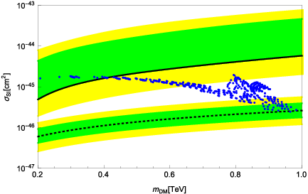
When discussing the scale phase transition at finite temperature and the GW background, we will consider a benchmark point in our parameter space:

which yields

As we can see from Fig. 1, most of the predicted points in the $m_{\rm DM}-\sigma_{SI}$ plane, except for those with smaller $m_{\rm DM}$, are close to the benchmark point. The third role of $\lambda_{HS}$ will be discussed when considering phase transition at finite temperature below.

It is expected that at high temperature the thermal effects restore the electroweak symmetry and scale symmetry. We assume that even at finite temperature the mean-field approximation is still a good approximation to the original strongly interacting gauge theory (1). The effective potential consists of four components,

where $V_{\text{MFA}}\!\left(f,h\right)$ and $V_{\text{CW}}\!\left(h\right)$ are given in (17) and (26), respectively. Since the absolute minimum of $V_{\text{MFA}}$ is located at $\langle\bar{S}\rangle=0$, we suppress the $\bar{S}$ dependence of $V_{\text{MFA}}$. The main thermal effects are included in $V_{\text{FT}}\!\left(f,h,T\right)$, which is

where $\omega_{I}=\sqrt{\vec{k}^{2}+m_{I}^{2}\!\left(h\right)}$, and the thermal masses are given by

Here $g_{2}=0.65$ and $g_{1}=0.36$ are the $SU(2)_{L}$ and $U(1)_{Y}$ gauge coupling constants, respectively, while $y_{t}=1.0$ stands for the top-Yukawa coupling constant. Further, $M^{2}$ and $\tilde{m}_{I}(I=W,Z,t,h)$ are given in (10) (with $H^{\dagger}H=h^{2}/2$) and (28), respectively. The thermal functions and their high temperature expansions are

Although the high temperature expansions are useful, they are not suitable for large $r>2$. Therefore, the following fitting functions [109] are used⁵⁵ 5 The validness of the approximations for the thermal functions is discussed in [110].:

The contribution from the ring (daisy) diagrams of gauge boson is [111]

where

Note that the ring contributions from the scalar $S$ and the Higgs field are included in (34).

Using the thermal effective potential (33), it is possible to consider phase transitions at finite temperature: There exist two phase transitions in this model, the scale and EW phase transitions (whose critical temperatures are denoted by $T_{\text{S}}$ and $T_{\text{EW}}$, respectively). The scale phase transition in hidden sector can be strongly first-order for a wide range in the parameter space [64]. In the case with $N_{f}=1$ (no DM) we see that both phase transitions can be strongly first-order and occur at the same temperature, $T_{\text{S}}=T_{\text{EW}}$. On the other hand, if DM is consistently included ($N_{f}>1$), the EW phase transition becomes weak, although the scale phase transition is still strongly first-order, and $T_{\text{EW}}<T_{\text{S}}$. The crucial difference between the two cases comes from the value of the Higgs portal coupling constant $\lambda_{HS}$, which controls the strength of the connection between the SM and hidden sector. As discussed in section III, smaller $\lambda_{HS}$ means larger $\Lambda_{H}$, which in turn implies larger $T_{S}$, while $T_{\text{EW}}$ stays around $O(100)$ GeV. This is the third role of $\lambda_{HS}$. Therefore, within the minimal model with a DM candidate we are considering here, the scale phase transition occurs at a higher temperature than the EW phase transition and is strongly first-order. Since we are especially interested in the possibility to explain the origin of the EW scale and DM at the same time, we focus in the following discussions on the model with $N_{f}=2$, in which, as explained in section III, the weakest constraint on $\lambda_{HS}$ has to be satisfied.

The EW phase transition is shown in Fig. 3 for the set of the benchmark parameters (31). We see from Fig. 3 that a weak transition appears around $T_{\text{EW}}\simeq 0.161$ TeV. Fig. 4 (left) presents $\langle f\rangle^{1/2}/T$ as a function of $T$, while Fig. 4 (right) shows the effective potential $V_{\text{eff}}$ given in (33) with $h=0$ at $T=T_{S}=0.323$ TeV as a function of $f^{1/2}$, showing that the scale phase transition is strongly first-order.

As we have seen in the previous section, the scale phase transition occurs at $T\mathrel{\mathchoice{\vbox{\halign{$\m@th\displaystyle\hfil#\hfil$\cr<\crcr\sim\crcr}}}{\vbox{\halign{$\m@th\textstyle\hfil#\hfil$\cr<\crcr\sim\crcr}}}{\vbox{\halign{$\m@th\scriptstyle\hfil#\hfil$\cr<\crcr\sim\crcr}}}{\vbox{\halign{$\m@th\scriptscriptstyle\hfil#\hfil$\cr<\crcr\sim\crcr}}}}$ few hundred GeV. This is larger than $T_{\text{EW}}$, and moreover the phase transition is strongly first-order⁶⁶ 6 The GW background produced by a strong EW phase transition has been studied in [112, 113, 114, 115, 116, 117, 118, 119]. Similar studies have been made in [120, 121].. This strong first-order phase transition produces the EW scale and at the same time dark matter in the early Universe. Fortunately, this phase transition could be observed indirectly, because it can generates stochastic GW background, which can be detected in GW experiments [65, 66, 67]. The most important quantity in studying the GW relics is the GW background spectrum (see for instance [68, 69]) $\Omega_{\text{GW}}\!\left(\nu\right)\sim\frac{d\rho_{\text{GW}}}{d\log\nu}$, where $\nu$ is the frequency of the GW, and $\rho_{\text{GW}}$ is the energy density of the GW. The energy density $\rho_{\text{GW}}$ is proportional to $\langle\dot{h}_{ij}\dot{h}_{ij}\rangle$, where $h_{ij}$ is the transverse, traceless, spatial tensor perturbation of the Robertson–Walker metric, and the dot on $h_{ij}$ denotes the derivative with respect to time. The evolution of $h_{ij}$ is described by the Einstein equation with the energy-momentum tensor which contains the information about the phase transitions.

The characteristics of a first-oder phase transition in discussing the GW background spectrum are the duration of the phase transition and the latent heat released. The duration time has to be sufficiently short compared with the expansion of the Universe, and it is clear that the more latent heat is released, the larger $\Omega_{\text{GW}}$ can become. In the following two subsections we will discuss these issues.

References

- [1] J. P. Fatelo, J. M. Gerard, T. Hambye and J. Weyers, Phys. Rev. Lett. 74 (1995) 492.
- [2] R. Hempfling, Phys. Lett. B 379 (1996) 153 [hep-ph/9604278].
- [3] T. Hambye, Phys. Lett. B 371 (1996) 87 [hep-ph/9510266].
- [4] K. A. Meissner and H. Nicolai, Phys. Lett. B 648 (2007) 312 [hep-th/0612165]; K. A. Meissner and H. Nicolai, Phys. Lett. B 660 (2008) 260 [arXiv:0710.2840 [hep-th]]; K. A. Meissner and H. Nicolai, Phys. Rev. D 80 (2009) 086005 [arXiv:0907.3298 [hep-th]].
- [5] R. Foot, A. Kobakhidze and R. R. Volkas, Phys. Lett. B 655 (2007) 156 [arXiv:0704.1165 [hep-ph]]; Phys. Rev. D 84 (2011) 075010 [arXiv:1012.4848 [hep-ph]].
- [6] R. Foot, A. Kobakhidze, K. .L. McDonald and R. .R. Volkas, Phys. Rev. D 76 (2007) 075014 [arXiv:0706.1829 [hep-ph]]; Phys. Rev. D 77 (2008) 035006 [arXiv:0709.2750 [hep-ph]]; Phys. Rev. D 89 (2014) 11, 115018 [arXiv:1310.0223 [hep-ph]].
- [7] W. -F. Chang, J. N. Ng and J. M. S. Wu, Phys. Rev. D 75 (2007) 115016 [hep-ph/0701254 [HEP-PH]].
- [8] T. Hambye and M. H. G. Tytgat, Phys. Lett. B 659 (2008) 651 [arXiv:0707.0633 [hep-ph]].
- [9] S. Iso, N. Okada and Y. Orikasa, Phys. Lett. B 676 (2009) 81 [arXiv:0902.4050 [hep-ph]]; Phys. Rev. D 80 (2009) 115007 [arXiv:0909.0128 [hep-ph]]; PTEP 2013 (2013) 023B08 [arXiv:1210.2848 [hep-ph]].
- [10] M. Holthausen, M. Lindner and M. A. Schmidt, Phys. Rev. D 82 (2010) 055002 [arXiv:0911.0710 [hep-ph]].
- [11] K. Ishiwata, Phys. Lett. B 710, 134 (2012) [arXiv:1112.2696 [hep-ph]].
- [12] C. Englert, J. Jaeckel, V. V. Khoze and M. Spannowsky, JHEP 1304 (2013) 060 [arXiv:1301.4224 [hep-ph]].
- [13] T. Hambye and A. Strumia, Phys. Rev. D 88, 055022 (2013) doi:10.1103/PhysRevD.88.055022 [arXiv:1306.2329 [hep-ph]].
- [14] V. V. Khoze and G. Ro, JHEP 1310 (2013) 075 [arXiv:1307.3764].
- [15] C. D. Carone and R. Ramos, Phys. Rev. D 88 (2013) 055020 [arXiv:1307.8428 [hep-ph]].
- [16] A. Farzinnia, H. -J. He and J. Ren, Phys. Lett. B 727 (2013) 141 [arXiv:1308.0295 [hep-ph]].
- [17] F. Gretsch and A. Monin, arXiv:1308.3863 [hep-th].
- [18] Y. Kawamura, PTEP 2013 (2013) 11, 113B04 [arXiv:1308.5069 [hep-ph]].
- [19] V. V. Khoze, JHEP 1311 (2013) 215 [arXiv:1308.6338 [hep-ph]].
- [20] E. Gabrielli, M. Heikinheimo, K. Kannike, A. Racioppi, M. Raidal and C. Spethmann, Phys. Rev. D 89, 015017 (2014) [arXiv:1309.6632 [hep-ph]].
- [21] S. Abel and A. Mariotti, Phys. Rev. D 89 (2014) 12, 125018 [arXiv:1312.5335 [hep-ph]].
- [22] M. Ibe, S. Matsumoto and T. T. Yanagida, Phys. Lett. B 732 (2014) 214 [arXiv:1312.7108 [hep-ph]].
- [23] C. T. Hill, Phys. Rev. D 89 (2014) 7, 073003 [arXiv:1401.4185 [hep-ph]].
- [24] J. Guo and Z. Kang, arXiv:1401.5609 [hep-ph].
- [25] S. Benic and B. Radovcic, Phys. Lett. B 732 (2014) 91 [arXiv:1401.8183 [hep-ph]]; S. Benic and B. Radovcic, JHEP 1501 (2015) 143 [arXiv:1409.5776 [hep-ph]].
- [26] V. V. Khoze, C. McCabe and G. Ro, JHEP 1408 (2014) 026 [arXiv:1403.4953 [hep-ph], arXiv:1403.4953].
- [27] A. Salvio and A. Strumia, JHEP 1406, 080 (2014) [arXiv:1403.4226 [hep-ph]].
- [28] H. Davoudiasl and I. M. Lewis, Phys. Rev. D 90 (2014) 3, 033003 [arXiv:1404.6260 [hep-ph]].
- [29] P. H. Chankowski, A. Lewandowski, K. A. Meissner and H. Nicolai, Mod. Phys. Lett. A 30 (2015) 02, 1550006 [arXiv:1404.0548 [hep-ph]].
- [30] K. Allison, C. T. Hill and G. G. Ross, Phys. Lett. B 738 (2014) 191 [arXiv:1404.6268 [hep-ph]]; K. Allison, C. T. Hill and G. G. Ross, Nucl. Phys. B 891 (2015) 613 [arXiv:1409.4029 [hep-ph]].
- [31] A. Farzinnia and J. Ren, Phys. Rev. D 90 (2014) 1, 015019 [arXiv:1405.0498 [hep-ph]].
- [32] P. Ko and Y. Tang, JCAP 1501 (2015) 023 [arXiv:1407.5492 [hep-ph]].
- [33] W. Altmannshofer, W. A. Bardeen, M. Bauer, M. Carena and J. D. Lykken, JHEP 1501 (2015) 032 [arXiv:1408.3429 [hep-ph]].
- [34] Z. Kang, arXiv:1411.2773 [hep-ph].
- [35] G. F. Giudice, G. Isidori, A. Salvio and A. Strumia, JHEP 1502 (2015) 137 [arXiv:1412.2769 [hep-ph]].
- [36] J. Guo, Z. Kang, P. Ko and Y. Orikasa, arXiv:1502.00508 [hep-ph].
- [37] K. Kannike, G. Hütsi, L. Pizza, A. Racioppi, M. Raidal, A. Salvio and A. Strumia, arXiv:1502.01334 [astro-ph.CO].
- [38] A. Ahriche, K. L. McDonald and S. Nasri, JHEP 1602 (2016) 038 [arXiv:1508.02607 [hep-ph]].
- [39] N. Haba, H. Ishida, N. Okada and Y. Yamaguchi, Phys. Lett. B 754 (2016) 349 [arXiv:1508.06828 [hep-ph]].
- [40] A. D. Plascencia, JHEP 1509, 026 (2015) doi:10.1007/JHEP09(2015)026 [arXiv:1507.04996 [hep-ph]].
- [41] V. V. Khoze and A. D. Plascencia, arXiv:1605.06834 [hep-ph].
- [42] A. Karam and K. Tamvakis, Phys. Rev. D 92, no. 7, 075010 (2015) doi:10.1103/PhysRevD.92.075010 [arXiv:1508.03031 [hep-ph]].
- [43] A. Karam and K. Tamvakis, Phys. Rev. D 94, no. 5, 055004 (2016) doi:10.1103/PhysRevD.94.055004 [arXiv:1607.01001 [hep-ph]].
- [44] S. R. Coleman and E. J. Weinberg, Phys. Rev. D 7 (1973) 1888.
- [45] Y. Nambu, Phys. Rev. Lett. 4 (1960) 380.
- [46] Y. Nambu and G. Jona-Lasinio, Phys. Rev. 122 (1961) 345; Phys. Rev. 124 (1961) 246.
- [47] T. Hur, D. -W. Jung, P. Ko and J. Y. Lee, Phys. Lett. B 696 (2011) 262 [arXiv:0709.1218 [hep-ph]].
- [48] T. Hur and P. Ko, Phys. Rev. Lett. 106 (2011) 141802 [arXiv:1103.2571 [hep-ph]].
- [49] M. Heikinheimo, A. Racioppi, M. Raidal, C. Spethmann and K. Tuominen, arXiv:1304.7006 [hep-ph].
- [50] M. Holthausen, J. Kubo, K. S. Lim and M. Lindner, JHEP 1312 (2013) 076 [arXiv:1310.4423 [hep-ph]].
- [51] J. Kubo, K. S. Lim and M. Lindner, Phys. Rev. Lett. 113 (2014) 091604 [arXiv:1403.4262 [hep-ph]].
- [52] J. Kubo, K. S. Lim and M. Lindner, JHEP 1409 (2014) 016 [arXiv:1405.1052 [hep-ph]].
- [53] O. Antipin, M. Redi and A. Strumia, JHEP 1501 (2015) 157 [arXiv:1410.1817 [hep-ph]].
- [54] M. Heikinheimo and C. Spethmann, JHEP 1412 (2014) 084 [arXiv:1410.4842 [hep-ph]].
- [55] C. D. Carone and R. Ramos, Phys. Lett. B 746 (2015) 424 [arXiv:1505.04448 [hep-ph]].
- [56] Y. Ametani, M. Aoki, H. Goto and J. Kubo, Phys. Rev. D 91, no. 11, 115007 (2015) [arXiv:1505.00128 [hep-ph]].
- [57] N. Haba, H. Ishida, N. Kitazawa and Y. Yamaguchi, Phys. Lett. B 755 (2016) 439 [arXiv:1512.05061 [hep-ph]].
- [58] K. Kannike, G. M. Pelaggi, A. Salvio and A. Strumia, JHEP 1607 (2016) 101 [arXiv:1605.08681 [hep-ph]].
- [59] H. Hatanaka, D. W. Jung and P. Ko, JHEP 1608 (2016) 094 [arXiv:1606.02969 [hep-ph]].
- [60] E. H. Fradkin and S. H. Shenker, Phys. Rev. D 19 (1979) 3682.
- [61] L. F. Abbott and E. Farhi, Phys. Lett. B 101 (1981) 69.
- [62] K. G. Chetyrkin, A. Y. Ignatiev, V. A. Matveev, M. E. Shaposhnikov and A. N. Tavkhelidze, Phys. Lett. B 117 (1982) 252.
- [63] J. Kubo and M. Yamada, Phys. Rev. D 93 (2016) no.7, 075016 [arXiv:1505.05971 [hep-ph]].
- [64] J. Kubo and M. Yamada, PTEP 2015 (2015) no.9, 093B01 [arXiv:1506.06460 [hep-ph]].
- [65] E. Witten, Phys. Rev. D 30 (1984) 272.
- [66] C. J. Hogan, Mon. Not. Roy. Astron. Soc. 218 (1986) 629.
- [67] M. S. Turner and F. Wilczek, Phys. Rev. Lett. 65 (1990) 3080.
- [68] M. Maggiore, Phys. Rept. 331 (2000) 283 doi:10.1016/S0370-1573(99)00102-7 [gr-qc/9909001].
- [69] P. Binetruy, A. Bohe, C. Caprini and J. F. Dufaux, JCAP 1206 (2012) 027 [arXiv:1201.0983 [gr-qc]].
- [70] T. Kahniashvili, A. Kosowsky, G. Gogoberidze and Y. Maravin, Phys. Rev. D 78, 043003 (2008) [arXiv:0806.0293 [astro-ph]].
- [71] C. Caprini et al., JCAP 1604 (2016) no.04, 001 [arXiv:1512.06239 [astro-ph.CO]].
- [72] P. Schwaller, Phys. Rev. Lett. 115 (2015) no.18, 181101 [arXiv:1504.07263 [hep-ph]].
- [73] B. P. Abbott et al. [LIGO Scientific and Virgo Collaborations], Phys. Rev. Lett. 116 (2016) no.6, 061102 [arXiv:1602.03837 [gr-qc]].
- [74] T. Hatsuda and T. Kunihiro, Prog. Theor. Phys. 71 (1984) 1332;
- [75] T. Hatsuda and T. Kunihiro, Phys. Rept. 247 (1994) 221 [hep-ph/9401310].
- [76] J. Hubbard, Phys. Rev. Lett. 3, 77 (1959).
- [77] R. L. Stratonovich, Sov.Phys.Dokl.,2,416 (1957).
- [78] A. Kosowsky, M. S. Turner and R. Watkins, Phys. Rev. D 45, 4514 (1992).
- [79] A. Kosowsky, M. S. Turner and R. Watkins, Phys. Rev. Lett. 69, 2026 (1992).
- [80] A. Kosowsky and M. S. Turner, Phys. Rev. D 47, 4372 (1993) [astro-ph/9211004].
- [81] M. Kamionkowski, A. Kosowsky and M. S. Turner, Phys. Rev. D 49, 2837 (1994) [astro-ph/9310044].
- [82] C. Caprini, R. Durrer and G. Servant, Phys. Rev. D 77, 124015 (2008) doi:10.1103/PhysRevD.77.124015 [arXiv:0711.2593 [astro-ph]].
- [83] S. J. Huber and T. Konstandin, JCAP 0809, 022 (2008) [arXiv:0806.1828 [hep-ph]].
- [84] R. Jinno and M. Takimoto, arXiv:1605.01403 [astro-ph.CO].
- [85] A. Kosowsky, A. Mack and T. Kahniashvili, Phys. Rev. D 66, 024030 (2002) [astro-ph/0111483].
- [86] A. D. Dolgov, D. Grasso and A. Nicolis, Phys. Rev. D 66, 103505 (2002) [astro-ph/0206461].
- [87] C. Caprini and R. Durrer, Phys. Rev. D 74, 063521 (2006) [astro-ph/0603476].
- [88] G. Gogoberidze, T. Kahniashvili and A. Kosowsky, Phys. Rev. D 76, 083002 (2007) [arXiv:0705.1733 [astro-ph]].
- [89] T. Kahniashvili, L. Campanelli, G. Gogoberidze, Y. Maravin and B. Ratra, Phys. Rev. D 78, 123006 (2008) Erratum: [Phys. Rev. D 79, 109901 (2009)] [arXiv:0809.1899 [astro-ph]].
- [90] C. Caprini, R. Durrer and G. Servant, JCAP 0912, 024 (2009) [arXiv:0909.0622 [astro-ph.CO]].
- [91] L. Kisslinger and T. Kahniashvili, Phys. Rev. D 92, no. 4, 043006 (2015) [arXiv:1505.03680 [astro-ph.CO]].
- [92] M. Hindmarsh, S. J. Huber, K. Rummukainen and D. J. Weir, Phys. Rev. Lett. 112, 041301 (2014) [arXiv:1304.2433 [hep-ph]].
- [93] M. Hindmarsh, S. J. Huber, K. Rummukainen and D. J. Weir, Phys. Rev. D 92, no. 12, 123009 (2015) [arXiv:1504.03291 [astro-ph.CO]].
- [94] J. T. Giblin, Jr. and J. B. Mertens, JHEP 1312, 042 (2013) [arXiv:1310.2948 [hep-th]].
- [95] J. T. Giblin and J. B. Mertens, Phys. Rev. D 90, no. 2, 023532 (2014) [arXiv:1405.4005 [astro-ph.CO]].
- [96] N. Seto, S. Kawamura and T. Nakamura, Phys. Rev. Lett. 87 (2001) 221103 [astro-ph/0108011]; S. Kawamura et al., Class. Quant. Grav. 23 (2006) S125; S. Kawamura et al., Class. Quant. Grav. 28 (2011) 094011.
- [97] C. G. Callan, Jr., Phys. Rev. D 2 (1970) 1541; K. Symanzik, Commun. Math. Phys. 18 (1970) 227.
- [98] H. Aoki and S. Iso, Phys. Rev. D 86 (2012) 013001 [arXiv:1201.0857 [hep-ph]].
- [99] J. H. Lowenstein and W. Zimmermann, Commun. Math. Phys. 46 (1976) 105; Commun. Math. Phys. 44 (1975) 73 [Lect. Notes Phys. 558 (2000) 310].
- [100] E. C. Poggio and H. R. Quinn, Phys. Rev. D 14 (1976) 578.
- [101] S. R. Coleman, R. Jackiw and H. D. Politzer, Phys. Rev. D 10 (1974) 2491.
- [102] M. Kobayashi and T. Kugo, Prog. Theor. Phys. 54 (1975) 1537.
- [103] L. F. Abbott, J. S. Kang and H. J. Schnitzer, Phys. Rev. D 13 (1976) 2212.
- [104] W. A. Bardeen and M. Moshe, Phys. Rev. D 28 (1983) 1372; Phys. Rev. D 34 (1986) 1229.
- [105] P. A. R. Ade et al. [Planck Collaboration], arXiv:1502.01589 [astro-ph.CO].
- [106] D. S. Akerib et al., arXiv:1608.07648 [astro-ph.CO]; D. S. Akerib et al. [LUX Collaboration], Phys. Rev. Lett. 112, 091303 (2014) [arXiv:1310.8214 [astro-ph.CO]]; D. S. Akerib et al. [LUX Collaboration], Phys. Rev. Lett. 116 (2016) no.16, 161301 [arXiv:1512.03506 [astro-ph.CO]].
- [107] E. Aprile [XENON1T Collaboration], Springer Proc. Phys. 148, 93 (2013) [arXiv:1206.6288 [astro-ph.IM]].
- [108] E. Aprile et al. [XENON Collaboration], JCAP 1604, no. 04, 027 (2016) [arXiv:1512.07501 [physics.ins-det]].
- [109] K. Funakubo and E. Senaha, Phys. Rev. D 79 (2009) 115024 [arXiv:0905.2022 [hep-ph]].
- [110] Y. Hamada and M. Yamada, arXiv:1605.06897 [hep-ph].
- [111] M. E. Carrington, Phys. Rev. D 45 (1992) 2933.
- [112] C. Grojean, G. Servant and J. D. Wells, Phys. Rev. D 71 (2005) 036001 [hep-ph/0407019]; C. Grojean and G. Servant, Phys. Rev. D 75 (2007) 043507 [hep-ph/0607107].
- [113] J. Kehayias and S. Profumo, JCAP 1003 (2010) 003 doi:10.1088/1475-7516/2010/03/003 [arXiv:0911.0687 [hep-ph]].
- [114] L. Leitao, A. Megevand and A. D. Sanchez, JCAP 1210 (2012) 024 [arXiv:1205.3070 [astro-ph.CO]].
- [115] Y. Kikuta, K. Kohri and E. So, arXiv:1405.4166 [hep-ph].
- [116] R. Jinno, K. Nakayama and M. Takimoto, Phys. Rev. D 93 (2016) no.4, 045024 [arXiv:1510.02697 [hep-ph]].
- [117] L. Leitao and A. Megevand, JCAP 1605 (2016) no.05, 037 [arXiv:1512.08962 [astro-ph.CO]].
- [118] M. Kakizaki, S. Kanemura and T. Matsui, Phys. Rev. D 92 (2015) no.11, 115007 [arXiv:1509.08394 [hep-ph]]; K. Hashino, M. Kakizaki, S. Kanemura and T. Matsui, Phys. Rev. D 94 (2016) no.1, 015005 [arXiv:1604.02069 [hep-ph]]; K. Hashino, M. Kakizaki, S. Kanemura, P. Ko and T. Matsui, arXiv:1609.00297 [hep-ph].
- [119] R. Jinno and M. Takimoto, arXiv:1604.05035 [hep-ph].
- [120] J. Jaeckel, V. V. Khoze and M. Spannowsky, arXiv:1602.03901 [hep-ph].
- [121] P. S. B. Dev and A. Mazumdar, Phys. Rev. D 93 (2016) no.10, 104001 [arXiv:1602.04203 [hep-ph]].
- [122] A. D. Linde, Nucl. Phys. B 216 (1983) 421 Erratum: [Nucl. Phys. B 223 (1983) 544].
- [123] M. Shirogane, S. Ejiri, R. Iwami, K. Kanaya and M. Kitazawa, Phys. Rev. D 94 (2016) no.1, 014506 [arXiv:1605.02997 [hep-lat]].
- [124] A. Petiteau, http://www.apc.univ-paris7.fr/Downloads/lisa/eLISA/Sensitivity/Cfgv1/StochBkgd/