Wigner crystal phases in confined carbon nanotubes
Abstract
We present a detailed theoretical analysis of the Wigner crystal states in confined semiconducting carbon nanotubes. We show by robust scaling arguments as well as by detailed semi-microscopic calculations that the effective exchange interaction has an SU(4) symmetry, and can reach values even as large as in weakly screened, small diameter nanotubes, close to the Wigner crystal - electron liquid crossover. Modeling the nanotube carefully and analyzing the magnetic structure of the inhomogeneous electron crystal, we recover the experimentally observed ’phase boundaries’ of Deshpande and Bockrath [V. V. Deshpande and M. Bockrath, Nature Physics 4, 314 (2008)]. Spin-orbit coupling only slightly modifies these phase boundaries, but breaks the spin symmetry down to SU(2)SU(2), and in Wigner molecules it gives rise to interesting excitation spectra, reflecting the underlying SU(4) as well as the residual SU(2)SU(2) symmetries.
I Introduction
Electrons interacting through simple Coulomb interaction represent a most fundamental, nevertheless challenging interacting quantum system. Apart from dimensionality (), the behavior of a Coulomb gas depends on just two parameters: the temperature , and the strength of the Coulomb interaction relative to the electrons’ kinetic energy, characterized by the dimensionless ratio [1]
| (1) |
with denoting the electron density, the electrons’ effective mass, and the dielectric constant of the environment through which electrons interact.
While at very high temperatures electrons form a (almost) classical plasma, the behavior of the gas at low temperatures depends on the specific value of . At large densities corresponding to , the Coulomb interaction plays a minor role in dimensions, and Landau’s Fermi liquid state emerges as the temperature is lowered. At small densities (), however, interactions become strong and relevant. In this limit, translational symmetry is broken, electrons localize at low temperatures, and form a Wigner crystal, characterized by magnetic ordering [2, 3, 4].
While the three-dimensional picture of the previous paragraph applies also to two dimensions [5, 6, 7, 8, 9], it fails in one dimension, where quantum fluctuations destroy the long ranged charge order, remove the phase transition(s) 11 1 Several intruding magnetic phases have been proposed, preempting a direct transition between the Wigner crystal and the Fermi liquid state. between the crystalline and the liquid phases, and replace it by a smooth crossover at some value [11, 12]. Though there is no phase transition in one dimension, the physical picture is quite different in the dilute, , and dense regimes, . In the Wigner crystal regime, , the density-density correlation function reveals charges localized relative to each other, reflected in deep and long-ranged periodic oscillations [13, 12, 14]. In contrast, in the weakly interacting limit, , these oscillations become weak perturbations on a non-oscillating background 22 2 In case of screening, both regimes can be described as a Luttinger liquid. However, while the charge- and spin velocities are about the same for , the spin velocity gets exponentially suppressed compared to the charge velocity in the Wigner crystal regime,.. These differences are even more pronounced in a finite system, where charges are typically pinned by some walls or confining potentials, and a true Wigner crystal structure emerges at small densities [16, 14, 17].
In a recent experiment, Deshpande and Bockrath reported the (indirect) observation of a Wigner crystal state in a suspended carbon nanotube with a presumably confinement induced gap [18, 19]. In a finite magnetic field, they have observed oscillations in the addition energy of holes in a p-type nanotube, and argued that only a Wigner crystal picture is able to account for these oscillations systematically (see Fig. 1 for their ’phase diagram’). More recently, an isolated two-electron Wigner molecule has been observed in an ultraclean carbon nanotube [20]. In the latter experiments, the observed level structure has been supported by detailed ’ab initio’ calculations, evidencing an exchange splitting much below the single particle level spacing, a clear indication of the Wigner crystal regime. In addition to these experiments, circumstantial evidence to support the formation of a Wigner crystal in one-dimensional wires has also been reported recently by other experimental groups [21, 22, 23]. It has been suggested in Ref. [21], e.g., that Wigner crystallization accounts for the negative Coulomb drag effect observed in coupled parallel quantum wires.
Although for the experiments of Ref. [18] the Wigner crystal picture seemed to provide a coherent explanation, a sufficiently ’microscopic’ theoretical description of the nanotube’s Wigner crystal state was missing. Furthermore, in several other experiments [24, 25] a single-particle or mean field scenario, or eventually a Luttinger liquid picture appears to be sufficient [26, 27, 28]. The goal of the present work is to provide a detailed and quantitative theoretical description of an inhomogeneous Wigner crystal in a gapped carbon nanotube, to investigate its intriguing spin and pseudospin (chirality) physics, and to make a comparison with the experimental findings of Ref. [18]. For this purpose, we use a bottom-up approach. We start out from a detailed microscopic modeling of the nanotube, similar to Ref. [14], and extract the effective exchange interaction of two neighboring electrons in the Hartree field of all other electrons from their two-electron spectrum. Exchange processes involve both the spin () and chiral spin () of the the crystallized electrons, and an almost perfectly SU(4)-symmetric exchange interaction is recovered [29, 30]. We then determine the positions of the crystallized electrons self-consistently at the classical level and, having the separation dependence of the exchange coupling in hand, arrive at an effective exchange Hamiltonian,
| (2) |
with the operators and exchanging the spin and the chiral spin of neighboring electrons in the crystal and . Although the exchange Hamiltonian possesses SU(4) symmetry, this symmetry is broken to SU(4)SU(2)SU(2) by the spin-orbit (SO) coupling [31, 32, 33, 34]. The spin-orbit coupling between the motion of the particles around the tube and their spin can be taken into account by the term
| (3) |
with and denoting the chirality and spin of the th localized electron, respectively, and the spin-orbit splitting. We use the effective Hamiltonians Eq. (2) and Eq. (3) first to construct and classify the low energy excitations of Wigner molecules, and then to construct the ’phase diagram’ of a parabolically confined Wigner crystal in a magnetic field by means of an inhomogeneous valence bond approach [27].
The final ’phase diagram’, constructed from the magnetization jumps between different charging states of the nanotube is summarized in Fig. 1 (and discussed in Section IV). Our theoretical ’phase diagram’ compares astonishingly well with the experimentally determined phase boundaries in Ref. [18]. Our calculations rely on just a few parameters, estimated from the experimental data: the radius of the nanotube, yielding the experimentally reported curvature induced gap [35], the dielectric constant , the strength of a parabolic confinement potential , defined in Eq. (13) and determined from the addition energy spectra (see Ref. [36] and Appendix D for details), and the measured orbital magnetic moment (-factor). We thus have one unknown parameter, the dielectric constant . The value of incorporates various screening effects including that of plasmonic excitations and, depending on the specific arrangements and the chirality of the nanotube, can take very different values [37]. Throughout this paper we use the value observed in suspended nanotubes [38] and suspended low density graphene [39], , incorporating short distance screening effects. The choice would also appear to be natural [40], however, as we discuss later, this value seems to be inconsistent with the experimental observations of Ref. [18].
We also find that for these parameters, supported by the experimental data of Ref. [18], the Wigner crystal picture can be appropriate up to around electrons, where the Wigner crystal starts to ’melt’. The crossover from the Wigner crystal to the electron liquid regime occurs at a crossover value , which we estimate based upon exact diagonalization calculations similar to those in Ref. [14] to be (see also Section V). At this crossover value of (the boundary of the Wigner crystal regime) the one-dimensional density of the electrons (holes) and their exchange coupling scale as
| (4) |
The effective mass of a semiconducting nanotube depends sensitively on the radius of the nanotube, . Therefore, the precise density range of Wigner crystal behavior as well as the energy scale of the exchange interaction in the Wigner crystal regime are very sensitive to the radius of the tube as well as the precise value of . For a nanotube of radius and , detailed estimates yielded a relatively small exchange coupling and a large crossover separation [20]. On the other hand, for a nanotube of radius (yielding a band gap close to the one reported in Ref. [18]), and of moderate screening, , Eq. (4) immediately yields a surprisingly large ’crossover’ exchange coupling along with a small carrier separation,
| (5) |
We thus conclude that the first transition line in Fig. 1 occurs well within the Wigner crystal regime, supporting the interpretation of the authors of Ref. [18], while the second transition line reaches into the melted region for high magnetic fields. We emphasize, however, that stronger screening by the environment, quickly reduces to the few Kelvin range, and increases simultaneously the characteristic separation of particles to .
The rest of the paper is structured as follows: In Sec. II we determine the effective exchange interaction between two neighboring electrons in the Wigner crystal state and construct the effective spin Hamiltonian of a one dimensional electron crystal in the nanotube. In Sec. III we analyze the magnetic excitations of small Wigner molecules and show how spin-orbit interaction breaks the SU(4) symmetrical spectrum to SU(2)SU(2) multiplets. In Sec. IV we investigate the spin structure of confined inhomogeneous nanotubes in an external magnetic field using a fermionic valence-bond calculation. Finally, before concluding, in Sec. V we discuss the limitations and consistency of the Wigner crystal approach and present the simple scaling arguments, leading to the relations Eq. (4). Four appendices explain some useful details of these calculations.
II Construction of the effective Hamiltonian
II.1 Derivation of the exchange coupling
To determine the exchange coupling in the Wigner crystal regime, we use a bottom-up approach. First, we model the interaction of two neighboring electrons in detail by semi-microscopic calculations [14], and extract their exchange interaction from the two-particle excitation spectrum. We find that the exchange interaction is quite accurately given by a semiclassical expression, similar to the ones used in Refs. [41, 42].
In small diameter semiconducting nanotubes discussed here, and at scales larger than the atomic scale, the motion of the interacting electrons (holes) is well described in terms of the lowest conduction (or highest valence) bands and the corresponding effective Hamiltonian
| (6) |
with and denoting the particles’ cylindrical coordinates (see also Appendix B) 33 3 Notice that after projection to the lowest conduction band, the kinetic energy contains only the coordinates , but the wave functions still have an angular dependence, as dictated by the chirality quantum number. The -dependence therefore still appears in the interaction-part of Eq. (6).. The effective mass here is simply related to the gap of the nanotube as with the Fermi velocity of graphene. For the sake of simplicity and concreteness, here we discuss electron-doped small radius semiconducting nanotubes, where the gap is mostly due to radial confinement and [35], but our discussion carries over with trivial modifications to hole-doping and nanotubes with strain or curvature induced gaps, too. In these latter cases, however, particles are typically lighter and it is harder to reach the Wigner crystal regime experimentally.
The Coulomb interaction
| (7) |
depends just on the distance between particles and thus and 44 4 A microscopic cut-off is usually also introduced to regularize it on the atomic scale (see Appendix B).. The dielectric constant depends crucially on the way the nanotube is prepared and contacted; for a nanotube laid over a typical semiconductor seems to be a reasonable estimate [45], while in suspended nanotubes it may get close to the vacuum value, and or possibly even smaller values seems to be a realistic choice [40, 45].
Consider now two neighboring particles in the Wigner crystal regime, moving in the Hartree field of the other particles, and interacting with each other as described by the effective Hamiltonian,
| (8) | |||||
The Hartree potential , displayed in Fig. 2, is well approximated in the Wigner crystal regime as
with the denoting the classically obtained locations of the other particles, and the angular averaged Coulomb interaction,
| (9) |
The angular dependence of the wave function is determined by the isospin (chirality) of the electrons, which also enters the two-particle wave function as , with the angular momentum determined by the chirality of the tube 55 5 For a gapped zig-zag nanotube of chirality , considered here, (). (details of the derivation are provided in Appendix A). The interaction term in Eq. (8) preserves the total isospin of the two interacting particles: , but the matrix elements of do depend on the relative values of and . Nevertheless, while for integration over the angles yields the effective interaction, , the off-diagonal matrix elements of the potential, are found to be several orders of magnitude smaller than for due to rapid oscillations of the wave functions [14]. Therefore, to a very good accuracy, the two-body Hamiltonian is diagonal in the spin and isospin quantum numbers, and the corresponding Schrödinger equation reads
| (10) |
with the total two-body potential.
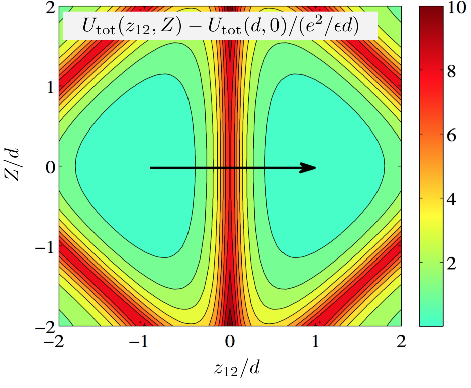
The chiral and spin quantum numbers are tied together with the orbital part of the wave function by Pauli’s principle. Spatially-even solutions of (10) imply antisymmetry under exchanges , while odd solutions must be symmetric under them. Therefore, the spectrum of the lowest 16 eigenstates of (10) is reproduced by the effective spin exchange Hamiltonian
| (11) |
with denoting the splitting of the 6-fold degenerate ground state and the 10-fold degenerate first excited multiplet. These large degeneracies are due to the (approximate) SU(4) symmetry of the exchange interaction.
The splitting can be extracted by diagonalizing the two-body Hamiltonian [47] or, alternatively, in the Wigner crystal regime one can determine it with a remarkable accuracy by means of a semiclassical approach (see Appendix C). Displaying the two-body potential in terms of the relative and center of mass coordinates and , we notice that the two particles move in a double-well potential (see Fig. 3). Tunneling processes along the tunneling path indicated in Fig. 3 lift the degeneracy of left and right states associated with the minima of , and give rise to the exchange splitting .
The couplings are displayed in Fig. 4 as a function of for several experimentally relevant nanotube radii and . In these density units, the boundary of the Wigner crystal is at independently of the radius of the nanotube (see Section V). For small radius nanotubes we find that the exchange coupling can be as high as before the crystal starts to ’melt’. This value can be even higher in case is closer to 1.
II.2 Effective spin Hamiltonian of a carbon nanotube Wigner crystal
Having determined the exchange coupling in a homogeneous gas of electrons, we are now in a position to construct an effective Wigner crystal Hamiltonian. Assuming that the density of the electron or hole gas changes relatively slowly on the scale of typical particle-particle separations and that charges are pinned by some confining potential, we can neglect charge fluctuations and approximate the exchange coupling of two neighboring particles as , with denoting their separation. We thereby arrive at the effective exchange Hamiltonian in Eq. (2).
The spin-orbit coupling, Eq. (3), does not influence the exchange coupling substantially, and we have therefore neglected it in the previous subsection. However, deeper in the Wigner crystal regime (or in screened nanotubes) it can be comparable with or larger, and can influence the spin state of the nanotube essentially [48]. The value of the coupling is roughly inversely proportional to the radius of the tube, , though sample to sample fluctuations can be large [35]. As already mentioned in the Introduction, breaks the SU(4) symmetry of the exchange Hamiltonian Eq. (2) down to . However, turns out to be relatively small in the crossover regime compared to the exchange coupling in poorly screened () nanotubes. For a nanotube of radius and , e.g., [35], which is about a factor smaller than the exchange coupling in the crossover regime.
The symmetry of the Wigner crystal state is further reduced in the presence of an external magnetic field. Here we focus on the simple case of a magnetic field parallel to the axis of the nanotube, when
| (12) |
with and the Bohr magneton. Thereby the symmetry of the crystal is further reduced to .
For an infinite nanotube the orbital -factor can be estimated as , however, this value can be substantially reduced by confinement [33]. Therefore, for the nanotube in Fig. 1 we have used the experimentally extracted -factor, , corresponding to [18], yielding indeed good agreement for the ’phase boundaries’ in Fig. 1.
III Wigner molecules
For small systems of and 3 electrons (holes) Wigner molecules form, and we can diagonalize the effective Hamiltonians Eqs. (2) and (3) analytically to obtain their spin excitation spectrum. For , the spectrum is organized into SU(4) multiplets characterized by Young tableaux. For a particle molecule, e.g., the lowest states are organized into a 6-fold degenerate antisymmetric ground state multiplet and a 10-fold degenerate symmetrical excited state (see Fig. 5).
These highly degenerate multiplets are split for , and can be classified by the residual SU(2)SU(2) symmetries, with their generators and inducing internal rotations within the subspaces. In terms of these latter, the 6-fold degenerate ground state is split to two singlet states, and a fourfold degenerate excited multiplet. In contrast, the 10-times degenerate excited state splits into a 4-fold degenerate multiplet, and two three-fold degenerate multiplets, and a for .
Injecting a third carrier into the nanotube, an -particle Wigner molecule forms. The Hilbert space of low-lying spin excitations is then -dimensional, these 64 states are, however, organized into just four SU(4) multiplets in the absence of : the 4-fold degenerate ground state is again completely antisymmetric in the united spin-isospin space, while excited multiplets have mixed symmetries and are all 20-fold degenerate. Similar to the case of the molecule, these states can be classified in terms of , too, and their spin-orbit coupling induced splitting and their energy can be exactly determined with group theoretical methods (see Fig. 6).
Injecting yet another carrier, an Wigner molecule forms. In this case, even if we assume that the Wigner molecule is symmetrical relative to its center, two distinct couplings need to be introduced, one for the central bond (), and another one for the two side bonds (). The excitation spectrum cannot be determined analytically in this case, but the ground state is found to be an SU(4) singlet, as expected.
The approximately SU(4) symmetrical molecular states should be visible in the molecules’ co-tunneling spectrum, and may lead to interesting quantum states when coupled to electrodes (see Summary and Conclusions) [49, 50]. The SU(4) spin, coupled to two (SU(4)) Luttinger liquids, e.g., could give rise to an SU(4) two-channel Kondo state, characterized by an anomalous scaling dimension [51]. Coupling the SU(4) Wigner molecule to side electrodes would, on the other hand, lead to an SU(4) Fermi liquid state 66 6 The exponent refers to the case of the SU(4)SU(2) model with Fermi liquid leads. This exponent is, however, expected to remain unchanged in the Luttinger liquid case, too, since correlators (i.e., spin excitations) in the SU(4) spin sector of the leads are expected to remain unaffected by the Luttinger parameter of the charge sector.. The higher dimensional SU(4) spins may give rise to exotic underscreened Kondo states.
IV Wigner crystal state in a parabolically confined nanotube
We now turn to the experimental setup of Ref. [18], where the nanotube was attached to source, drain and gate electrodes. In this case, the attached gate electrodes can produce Schottky barriers at the ends of the nanotube, and charges accumulated there are expected to create a smooth external, approximately parabolic confinement potential for the charge carriers:
| (13) |
The depth of the potential, can be estimated from the measured charging energy of the nanotube (see Appendix D for details). Throughout the present work we consider , which for corresponds to a charging energy of , in rough agreement with the value reported in Ref. [18], . For a nanotube this corresponds to a confinement energy .
In a parabolic confinement, the gas of particles is denser at the central region of the tube, and correspondingly, the exchange coupling is larger there, and decreases towards the ends of the tube. In the experiments the gate voltage is varied, and the number of the charge carrier increases one by one until the Wigner crystal gradually melts at the center of the tube. For each we therefore need to determine the dynamical rearrangement of the particles and, accordingly, a new distribution of the couplings . To this end, we minimized the classical Coulomb energy of the particles in the confining potential,
Fig. 7 shows the spatial dependence of the inhomogeneous couplings and the position dependent interaction parameter for charged particles in a nanotube of and . Remarkably, remains above the crossover value even at the center of the tube, where the exchange coupling is as large as , and the whole nanotube is in the Wigner crystal regime. For larger values, , however, becomes smaller that at the center of the nanotube, and the core of the Wigner crystal melts.
To determine the spin state of the relaxed Wigner crystal, we performed a valence bond mean field calculation. We first grouped the spin and isospin variables as , and rewrote the exchange interaction in a readily SU(4) invariant form as
| (14) |
with the fermionic operators () creating (annihilating) a carrier on site , and satisfying the constraint at each site. The operators obey the SU(N) commutation relations . The terms and can also be expressed in terms of the SU(4) spin operators, , and obviously break the SU(4) symmetry of . Notice that the Hamiltonian (14) is also invariant under local gauge transformations, , reflecting local particle number conservation.
In the presence of the terms and , the inhomogeneity in the exchange coupling plays a crucial role. For longer Wigner chains, the exchange coupling is very strong at the center of the chain, while at the wings it can be smaller by two or more orders of magnitude. Therefore, in the presence of an external magnetic field, the nanotube may be phase separated, with wings polarized in isospin and spin space, and the center of the chain remaining in an approximately SU(4) antiferromagnetic Néel state. For smaller external magnetic fields all three phases can be present in the nanotube: a spin-isospin polarized state at the wings, where the field-induced Zeeman and orbital splitting are much larger than the exchange coupling, an antiferrmagnetic state at the center, where the exchange coupling dominates over the magnetic field, and an orbitally polarized spin antiferromagnet between them.
This competition of and leads to the nontrivial ’phase diagram’ shown in Fig. 1, constructed in Ref. [18] by investigating the change in total magnetization while adding an extra particle in a magnetic field, , a quantity which can be directly extracted through transport measurements from the shift of the Coulomb blockade peaks in a magnetic field. To understand this ’phase diagram’ we must keep in mind that the Wigner crystal is inhomogeneous and therefore the density and the exchange coupling are both the largest at the center of the nanotube. Consider now adding particles to the nanotube in a fixed external magnetic field. For small particle numbers, the exchange coupling remains small even at the center of the nanotube, and both the spins and the isospins of the entering particles are found to be completely polarized (phase I). For increasing particle numbers, however, the density and thus the exchange coupling at the center start to become larger, and the latter exceeds the spin splitting of the SU(4) spins, induced by the external magnetic field, but remains still smaller than the orbital splitting, due to the difference in the electronic and orbital -factors. As a consequence, new particles enter with alternating spins but polarized isospin (isospin polarized spin antiferromagnet, phase II). Finally, for even larger particle numbers, the exchange coupling at the center of the tube dominates, and electrons enter with alternating spin and orbital spins (spin-isospin antiferromagnet, phase III). Notice that the three regions in Fig. 1 are not true ’phases’. In region II, e.g., the nanotube hosts two magnetic phases: an orbitally polarized spin antiferromagnet at the center, and regions of fully polarized spins and isospins on the wings.
To analyze the spin-isospin configurations of the confined Wigner crystal theoretically, we made use of a self-consistent valence bond approach, whereby we decouple the exchange term assuming a finite to obtain
| (15) |
Here the Lagrange multipliers ensure that particle number is conserved on the average at each site and, similar to the , must be determined self-consistently. Notice that, by the local gauge invariance of (14), the are not uniquely defined, and the energies of the ground states of remain invariant under the transformation . This simple mean field approach captures surprisingly well the properties of SU(4) and SU(2) antiferromagnets and, according to our findings, can also account for the ’phase diagram’ of the carbon nanotube Wigner crystal.
The ’phase diagram’ represented in Fig. 1 has been determined by performing self-consistent calculations for each magnetic field and for up to particles. As already stated in the Introduction, apart from , which we have set to to agree with the values reported so far in suspended graphene and nanotubes [39, 45], all parameters have been estimated from the experiments: The parameter can be estimated from the charging energy , and is found to be in the range (see Appendix D). Here we shall use the value yielding the closest resemblance to the experimental data of Ref. [18]. The radius is determined from the curvature-induced gap reported in Ref. [18] (and is directly related tho the effective mass, ), and yields a spin-orbit splitting (see Ref. [35]). Finally, we have used the experimentally measured value, [18].
Results of these simulations have been summarized in Fig. 1. Though the magnetization pattern may be not as systematic as the ones reported in Ref. [18], – possibly due to our approximate valence bond method, – the similarity and the correct location of the ’phase boundaries’ are, nevertheless, striking. The overall good agreement is, however, shaded by the fact that for these parameters the density of the electron crystal starts to exceed the crossover value for at the center (see Appendix D). A somewhat weaker confinement, increases this characteristic value of , and yields also a charging energy in better agreement with the experimentally observed value, but the agreement of the ’phase diagram’ in Fig. 1 gets worse.
V Range of validity of the Wigner crystal description and scaling relations
Throughout our previous analysis, we assumed that electrons are reasonably localized by their strong Coulomb interaction. While this assumption is certainly not correct for an infinite chain, where charge fluctuations are unlimited and no long-ranged charge order exists even at temperature, it can certainly be applied in a finite system, where charge fluctuations are pinned. Then our approach is valid under the condition that typical quantum fluctuations of the localized charges be less than their separation, .
The ratio is directly related to the parameter . Computing the width of a Gaussian wave function selfconsistently within the Coulomb potential of an infinite chain of particles yields the simple estimate (see Appendix B)
| (16) |
with the geometrical factor depending on the densities (wave functions) of the other localized charges. For perfectly localized particles we find , with the Zeta function (see Appendix B). However, the factor increases as one approaches the border of the Wigner crystal regime, , which we define as the value of , where the charge density is suppressed by a factor of 2 as one moves from one lattice position to the next one, a condition yielding for Gaussian wave packets. Smearing the electron charges then in boxes of width yields at the transition, corresponding to the rough estimate, .
A more accurate way to estimate is to perform calculations for a molecule in a harmonic trap, where one can squeeze the atoms together by increasing the confinement frequency [14]. The crossover density and thus can then be determined by just looking at the separation of the two charges when the charge density at the center is reduced by a factor of . This more accurate procedure yields the crossover value , used throughout this paper.
Now we show that at the crossover, , the exchange coupling and the density obey the scaling relations, Eq. (4). To prove this, we first observe that, according to our discussion in Sec. II.1, the electron-electron interaction can be replaced by the angular averaged interaction, in Eq. (9). Introducing the dimensionless coordinates, , the Hamiltonian of the interacting particles becomes
| (17) |
with the dimensionless Hamiltonian given by
| (18) |
where the dimensionless averaged Coulomb interaction trivially depends on the dimensionless parameter . Thus, in the dilute limit we have , and the structure of the dimensionless wave function and the energy spectrum of the dimensionless Hamiltonian depend only on . It follows immediately that at the crossover point, , the density of the gas scales as
| (19) |
while the exchange energy is just a universal number () apart from the overall energy scale in Eq. (17),
| (20) |
Eq. (20) just follows from the fact that, Ð in the spirit of the virial theorem, - at the crossover, the Coulomb, the kinetic, and the exchange energies are all approximately equal, while Eq. (19) states that the density of the gas is inversely proportional to the effective Bohr radius.
These general scaling relations hold under the condition . Using the relation [35] with (yielding, e.g., for a nanotube of radius ), this condition simplifies to
| (21) |
This inequality is well satisfied for even slightly screened nanotubes with , but we find that relations (4) are also obeyed by the exchange couplings and densities extracted from the two-body spectrum of unscreened nanotubes with , for which (21) is certainly only poorly satisfied.
VI Summary and conclusions
In this work, we attempted to account for the magnetic behavior of a Wigner crystal that forms in a confined semiconducting carbon nanotube. We have carefully estimated the exchange interaction () between neighboring localized electrons (holes) in the crystalline state, and have shown that it is SU(4) symmetric with very good accuracy. For poorly screened small diameter semiconducting nanotubes, the microscopically determined exchange couplings at the ’melting’ of the crystal turn out to be surprisingly large , . These large values follow from very robust scaling arguments, and are also in agreement with experiments [18, 20] as well as independent theoretical computations [14, 20], also reproduced here. As we argued, at the cross-over the exchange coupling is just proportional to the effective Bohr energy, with replaced by and with an additional factor , yielding the simple estimate, . Determining the numeric prefactor omitted here requires more accurate computations, but it is not unreasonable to assume it is in the range of . For a nanotube with and , this heuristic estimate gives to , consistent with our more accurate calculations.
Spin-orbit coupling () breaks the SU(4) spin symmetry down to SU(2)SU(2) [53]. As we demonstrated in Section III, for small, – particle Wigner molecules, the interplay between and leads to interesting spin excitation spectra with excited states classified as SU(2)SU(2) multiplets. This intriguing spin spectrum should readily be seen in the co-tunneling spectrum of Wigner molecules, would provide direct information on , , and would also evidence the underlying SU(4) and the residual SU(2)SU(2) symmetries.
The interesting spin structure of the molecule can lead to exciting quantum states when the molecule is coupled to electrodes [49, 50]. For small , the SU(4) spin, coupled to two (SU(4)) Luttinger liquids, e.g., may give rise to a SU(4) two-channel Kondo state, characterized by an anomalous scaling dimension [51]. Coupling the SU(4) Wigner molecule to side electrodes would, on the other hand, lead to an SU(4) Fermi liquid state, while higher dimensional SU(4) spins may give rise to exotic underscreened Kondo states. A finite will, however, induce a crossover to SU(2)SU(2) states, and lead to less exciting SU(2) Kondo physics at low temperatures.
We remark that the competition between and has even more exciting implications for homogeneous crystals [48]. The spin-orbit coupling breaks the original SU(4) spinon excitations of the SU(4) antiferromagnet into SU(2) spinons propagating with 3 different spin velocities, and leads to a quantum phase transition with one of the spinons becoming gapped as we move deeper into the Wigner crystal regime.
To test our semi-microscopic approach, we have performed a detailed modeling of the experiments of Ref. [18]. We estimated the basic model parameters (, and confinement strength ) directly from the experiments. We have set the unknown dielectric constant to [45]. Performing a self-consistent valence-bond calculation for an increasing number of electrons in an external magnetic field, we recovered the experimentally observed magnetic ’phase boundaries’ with reasonable accuracy. As we have discussed in Section IV, these ’phase boundaries’ from the inhomogeneity of the crystal, and do not correspond to new phases, rather they can be interpreted as the emergence of different types of antiferromagnetic domains at the center of the nanotube, where the density and thus the exchange coupling are both the largest. Given the simple multiscale calculations we performed, the good agreement with the experiments is striking.
We should remark though that while the ’phase boundaries’ we get are qualitatively and quantitatively very close to the experimentally observed ones, we do not observe regular two-fold magnetization patterns, our patterns are closer to the ones presented in the supplemental information of Ref. [18]. This may be a consequence of the valence-bond approach we employed or possibly the ’melting’ of the Wigner crystal for larger particle numbers, which for our parameters occurs at .
We should also comment here on the value of the value of the dielectric constant . It would be natural to assume that in a nanotube suspended in vacuum [39, 40, 45]. However such a small value of is inconsistent with the data. For , only a shallow parabolic confinement with can yield charging energies compatible with the experimentally reported values, (see Appendix D). For such shallow confinement the unscreened Coulomb repulsion pushes the charges quickly towards the end of the nanotube, and already for about they form a homogeneous crystal all over the nanotube. Such a homogeneous crystal is clearly incompatible with the experiments: in such a crystal exchange couplings are approximately equal, and a huge magnetization jump should occur at a critical magnetic field, , not seen experimentally. Furthermore, such a homogeneous Wigner crystal will not melt gradually, but would develop a sudden transition in the whole crystal once the melting condition is satisfied.
Thus the value seems to be incompatible with the experimental data. So are larger values of . For these large values a very large confinement would be needed to yield . By our scaling arguments, the exchange coupling should then be less than , clearly inconsistent with the high field phase boundary observed in Ref. [18] and the corresponding exchange coupling, . Furthermore, in this case the crystal would melt very quickly, once a few particles enter the tube.
We thus conclude that only seems to give a consistent explanation for the data reported in Ref. [18]. For this value of the first transition between the completely polarized state and the spin-antiferromagnet (see Fig 1) occurs well in the Wigner crystal regime, however, for the Wigner crystal should melt, and our approach becomes questionable. The description of this regime of a partially melted confined Wigner crystal and the crossover between the Wigner crystal and electron (Luttinger) liquid regimes is a true theoretical challenge.
While spin-orbit coupling gives rise to interesting spin excitations in small molecules, we find that for a semiconducting nanotube of radius , corresponding to the gap measured in Ref. [18], , does not have a large impact on the magnetic states within the ’phase diagram’. It eliminates the orbitally polarized phase at very small fields but, apart from that, the ’phase diagram’ remains almost identical to that of an SU(4) symmetrical Wigner crystal with .
Let us finally comment on the general implications of our results and their limitations. Although we focused on semiconducting (zig-zag) nanotubes, most of our considerations are very general, and also apply with trivial modifications to metallic tubes with curvature or strain induced band gaps and semiconducting nanotubes of other chirality. In particular, the scaling relations Eq. (4) are very general, and imply that the range of applicability of the Wigner crystal picture as well as the strength of the exchange coupling depend extremely sensitively on microscopic parameters of the tube and details of the experimental setup; to observe the Wigner crystal and its magnetic structure it is essential to avoid strong screening and to increase the effective mass of the particles as much as possible. In practical terms, small radius or strongly strained suspended nanotubes of are best to observe the detailed structure of the crystal. Correspondingly, while the nanotube studied in Ref. [18], is found to be in the Wigner crystal regime for electron numbers , metallic nanotubes with small strain-induced gap laid on or close to a substrate are extremely unlikely to host Wigner molecules, and should rather be described in terms of extended electron (hole) states.
Acknowledgements.
We would like to thank Shahal Ilani, Christoph Strunk, Milena Grifoni, and especially to András Pályi for important and fruitful discussions, and to Răzvan Chirla for the careful reading of the manuscript. This work has been supported by the Hungarian research grant OTKA K105149, by NSF DMR Grant No. 1603243 (LG) and by UEFISCDI Romanian Grant No. PN-II-RU-TE-2014-4-0432 (CPM).Appendix A Construction of the Wigner crystal state in a zig-zag carbon nanotube

In this Appendix we construct the microscopic wave function of the localized electrons forming the Wigner crystal. The Brillouin zone (BZ) of the underlying graphene sheet is represented in Fig. 8, with the two inequivalent Dirac points denoted as and . Rolling up the graphene into a carbon nanotube (CN) restricts the BZ to some parallel line segments [54], with their orientation dictated by the chirality of rolling the nanotube. Here, for simplicity, we consider semiconducting zig-zag CN’s with chirality and radius (; ). In this case, allowed states in the graphene BZ consist of segments of length parallel to the direction (vertical red lines in Fig. 8), and lowest lying excitations are on the segments closest to . The minimum energy point of these vertical segments is at the points with . For low density CNs it is enough to restrict ourself to these two segments, , indexed by the isospin quantum numbers . Along these lines, for small , excitations are massive Dirac fermions with a dispersion
| (22) |
with the Fermi velocity of graphene and the effective mass
| (23) |
The wave functions (of the unrolled nanotube) for the electrons (holes) can be expressed by Bloch’s theorem as . Here we explicitly separate the position vector into a two dimensional vector within the graphene sheet, , and a coordinate perpendicular to it. In cylindrical coordinates of the nanotube , and the wave functions along the line segment read
| (24) |
with . These wave functions describe particles of chirality circulating around the tube.
In the Wigner crystal, we create wave packets from the states (24)
| (25) |
with a Gaussian envelope, and the location of the wave packet along the nanotube. Assuming that only weakly depends on , we obtain the quasiparticle wave function at position
| (26) |
with the sign referring to electrons and holes, and representing the spin part of the wave function. The Bloch functions in (25) describe an almost homogenius background charge pattern, which varies only at the atomic scale, and can be ignored in many cases. We should emphasize that the single band approach presented here is only be valid for wide enough wave packets,
| (27) |
Appendix B The effective Coulomb potential
The Coulomb potential in cylindrical coordinates is
| (28) |
with the electron charge and the relative dielectric constant. In the exact diagonalization approach of Ref. [14] the microscopic cut-off describes a crossover between the Coulomb potential and a Hubbard-like short range interaction for , and was fixed to , with . Then, the average interaction felt by two electrons at a distance is
| (29) |
with a dimensionless function
| (30) |
given in terms of the complete elliptic integral of the first kind, [55]. The screening length in Eq. (30) is of the order , is much smaller than , and regularizes the potential in the limit , while for large distances, the usual Coulomb behavior is recovered,
| (31) |
The Hartree potential felt by particle is given by with
| (32) |
Deep in the Wigner crystal the wave functions are well localized, and to a good approximation
| (33) |
with given by Eq. (29). The resulting Hartree potential is shown in Fig. 9. A similar procedure yields the two-particle potential displayed in Fig. 2.
We now estimate the extension of the wave function in this Hartree potential. We first approximate by a Coulomb potential to obtain the following parabolic approximation by expanding (33),
with the separation of electrons and 77 7 For an infinite chain we have , a divergence compensated by the background of positive charges.. Solving the harmonic oscillator problem in this harmonic potential yields then the simple estimate, Eq. (16).
Appendix C Exchange interaction in a Wigner molecule
In this appendix we present the semiclassical approach to determine the exchange interaction , which we also compare with the results of exact diagonalization [14, 20]. We consider two interacting electrons of mass in a parabolic confining potential of frequency . The Schrödinger equation can be factorized in this case in terms of the relative () and center of mass () coordinates, . The center of mass motion is that of a harmonic oscillator of frequency , and is completely decoupled from the relative motion described by the single particle Hamiltonian,
| (34) |
with the reduced mass and the cut-off function in Eq. (30). With a good accuracy, we can set the parameter to zero. We can then make the Hamiltonian dimensionless by introducing the dimensionless coordinate, , with the non-interacting oscillator length, and dividing it by the natural energy scale, . In these units, the Hamiltonian becomes
| (35) |
with characterizing the strength of Coulomb interaction compared to that of the parabolic confinement,
| (36) |
Notice that in Eq. (36) is different from the usual , defined by Eq. (1).
The dimensionless potential in Eq. (35) displays two minima at , corresponding to the ground state positions of the classical particles. Close to these minima, the potential can be approximated by parabolas, and the molecule vibrates with a frequency , where is the second derivative with respect to . Tunneling processes between give rise to a splitting of these two levels, which we can identify as the exchange coupling. At the semiclassical level, we can thus estimate as the tunneling amplitude [1]
| (37) |
with denoting the classical turning-point determined by the equation . Alternatively, we can determine the spectrum of Eq. (35) numerically, and extract the ground state splitting from there.
Fig. 10 displays a comparison of the results of these two approaches as a function of for a nanotube of radius in a confining potential of frequency . Both approaches yield an exponential decay of with increasing . The semiclassical method slightly overestimates the exchange coupling, but it gives a surprisingly accurate estimate for . For a simple Coulomb interaction between the two electrons, (31), it estimates ’s within , but its accuracy remains around for the more appropriate nanotube interaction, Eq. (29), too.
Appendix D Charging energy of carbon nanotube in a confining potential
The Coulomb energy of a nanoscale object often depends approximately quadratically on the number of charged particles,
| (38) |
The charging energy can be directly extracted from the Coulomb diamonds. The data presented in Ref. [18], e.g., yield a value .
.
In this appendix we determine the effective value of as a function of the particle number for a CNT confined by a harmonic potential. Starting from the ansatz (38), the value of can be identified as the difference in the energy needed to add two consecutive electrons [36],
| (39) |
with , and the total energy of the CNT with confined charges.
In a parabolic confinement, the energy of a given classical charge configuration is the sum of the harmonic potential and the Coulomb energy,
| (40) |
For each , we first determine the coordinates of the particles by minimizing Eq. (40), and then compute the total energy . Introducing the dimensionless coordinates , with , the potential energy becomes
| (41) |
with the characteristic energy scale
As a consequence, can be expressed as We determined the universal function numerically, and displayed it in Fig. 11. It has a weak dependence on , and for particle numbers of interest , yielding the relation
This equation allows us to relate the screening parameter and the confinement parameter through the experimentally determined charging energy. For , used throughout this work, yield , roughly consistent with the data. For , however, one needs to use a much shallower confining potential with in order to be consistent with the experimentally observed charging energy.
In a finite nanotube of size , the ’length’ of the Wigner crystal increases monotonously with up to the size of the tube. In an infinite nanotube, the growth is universal and can be expressed as , with an universal function that we determined numerically. It is represented in the inset of Fig. 12. In the main panel of the same figure, we represent as function of the number of charges , for and as well as for and . While in the former case we can place about electrons on the nanotube before hitting the walls, in the ’unscreened’ case, , this number is only . Beyond this number the separation of the particles becomes quickly equidistant, yielding an almost uniform exchange coupling.
It is therefore evident that for large confinement potential depth and strong screening a far larger number of charges can be squeezed inside the nanotube, as decreases, but that’s not a guarantee that the Wigner crystal state survive as increases. The only relevant quantity that controls the ’melting point’ of the Wigner crystal is the dimensionless parameter . As displayed in inset of Fig. 7, for a given configuration with charges in the tube, is site dependent and has the smallest value in the middle of the chain. In Fig. 13 we represent in the middle of a long nanotube as function of the number of charges . When only a few charges are confined to the nanotube, the gas is diluted and, as expected, , but as the charges accumulate, decreases monotonously, and at some critical occupation it reaches , and the crystal starts to melt in the middle. Adding more charges, decreases further, and the melting progresses towards the sides of the chain.
References
- [1] K. A. Matveev, Phys. Rev. Lett. 92, 106801 (2004a).
- [2] E. Wigner, Phys. Rev. 46, 1002 (1934).
- [3] L. Bonsall and A. A. Maradudin, Phys. Rev. B 15, 1959 (1977).
- [4] L. Cândido, B. Bernu, and D. M. Ceperley, Phys. Rev. B 70, 094413 (2004).
- [5] F. M. Peeters, Phys. Rev. B 30, 159 (1984).
- [6] A. V. Filinov, M. Bonitz, and Y. E. Lozovik, Phys. Rev. Lett. 86, 3851 (2001).
- [7] V. J. Goldman, M. Santos, M. Shayegan, and J. E. Cunningham, Phys. Rev. Lett. 65, 2189 (1990).
- [8] S. Chakravarty, S. Kivelson, C. Nayak, and K. Voelker, Philosophical Magazine Part B 79, 859 (1999).
- [9] C. C. Grimes and G. Adams, Phys. Rev. Lett. 42, 795 (1979).
- [10] Several intruding magnetic phases have been proposed, preempting a direct transition between the Wigner crystal and the Fermi liquid state.
- [11] H. J. Schultz, Phys. Rev. Lett. 71, 1864 (1993).
- [12] J. S. Meyer and K. A. Matveev, Journal of Physics: Condensed Matter 21, 023203 (2009).
- [13] G. Piacente, I. V. Schweigert, J. J. Betouras, and F. M. Peeters, Phys. Rev. B 69, 045324 (2004).
- [14] A. Secchi and M. Rontani, Phys. Rev. B 82, 035417 (2010).
- [15] In case of screening, both regimes can be described as a Luttinger liquid. However, while the charge- and spin velocities are about the same for , the spin velocity gets exponentially suppressed compared to the charge velocity in the Wigner crystal regime,.
- [16] L. I. Glazman, I. M. Ruzin, and B. I. Shklovskii, Phys. Rev. B 45, 8454 (1992).
- [17] K. A. Guerrero-Becerra and M. Rontani, Phys. Rev. B 90, 125446 (2014).
- [18] V. V. Deshpande and M. Bockrath, Nat Phys 4, 314 (2008).
- [19] A gap in a nanotube can be induced by strain and curvature [35], too, but the relatively large gap reported in Ref. [18] is most likely due to confinement.
- [20] S. Pecker, F. Kuemmeth, A. Secchi, M. Rontani, D. Ralph, P. McEuen, and S. Ilani, Nat. Phys. 9, 576 (2013).
- [21] M. Yamamoto, M. Stopa, Y. Tokura, Y. Hirayama, and S. Tarucha, Science 313, 204 (2006).
- [22] W. K. Hew, K. J. Thomas, M. Pepper, I. Farrer, D. Anderson, G. A. C. Jones, and D. A. Ritchie, Phys. Rev. Lett. 102, 056804 (2009).
- [23] M. Yamamoto, H. Takagi, M. Stopa, and S. Tarucha, Phys. Rev. B 85, 041308 (2012).
- [24] U. Meirav, M. A. Kastner, M. Heiblum, and S. J. Wind, Phys. Rev. B 40, 5871 (1989).
- [25] A. N. Aleshin, H. J. Lee, Y. W. Park, and K. Akagi, Phys. Rev. Lett. 93, 196601 (2004).
- [26] T. Giamarchi, Quantum Physics in One Dimension (Oxford University Press, 2003).
- [27] L. S. Levitov and A. M. Tsvelik, Phys. Rev. Lett. 90, 016401 (2003).
- [28] V. V. Deshpande, M. Bockrath, L. I. Glazman, and A. Yacoby, Nature 464, 209 (2010).
- [29] B. Sutherland, Phys. Rev. B 12, 3795 (1975).
- [30] Y. Q. Li, M. Ma, D. N. Shi, and F. C. Zhang, Phys. Rev. Lett. 81, 3527 (1998).
- [31] T. Ando, Journal of the Physical Society of Japan 69, 1757 (2000).
- [32] D. Huertas-Hernando, F. Guinea, and A. Brataas, Phys. Rev. B 74, 155426 (2006).
- [33] T. Jespersen, Grove, J. Paaske, K. Muraki, T. Fujisawa, J. Nygard, and K. Flensberg, Nat Phys 7, 348 (2011).
- [34] F. Kuemmeth, S. Ilani, D. Ralph, and P. McEuen, Nature 452, 448 (2008).
- [35] E. A. Laird, F. Kuemmeth, G. A. Steele, K. Grove-Rasmussen, J. Nygård, K. Flensberg, and L. P. Kouwenhoven, Rev. Mod. Phys. 87, 703 (2015).
- [36] S. Sapmaz, P. Jarillo-Herrero, L. P. Kouwenhoven, and H. S. J. van der Zant, Semiconductor Science and Technology 21, S52 (2006).
- [37] B. Kozinsky and N. Marzari, Phys. Rev. Lett. 96, 166801 (2006).
- [38] Y. Miyauchi, R. Saito, K. Sato, Y. Ohno, S. Iwasaki, T. Mizutani, J. Jiang, and S. Maruyama, Chemical Physics Letters 442, 394 (2007).
- [39] F. Guinea, M. Katsnelson, and A. Geim, Nat Phys 6, 30 (2010).
- [40] In suspended nanotubes charge distributions seem to be consistent with . (S. Ilani, private communication.).
- [41] W. Häusler, Z. Physik B Cond. Matt. 99, 551 (1995).
- [42] K. A. Matveev, Phys. Rev. B 70, 245319 (2004b).
- [43] Notice that after projection to the lowest conduction band, the kinetic energy contains only the coordinates , but the wave functions still have an angular dependence, as dictated by the chirality quantum number. The -dependence therefore still appears in the interaction-part of Eq. (6).
- [44] A microscopic cut-off is usually also introduced to regularize it on the atomic scale (see Appendix B).
- [45] Y. Homma, S. Chiashi, and Y. Kobayashi, Reports on Progress in Physics 72, 066502 (2009).
- [46] For a gapped zig-zag nanotube of chirality , considered here, ().
- [47] Multiparticle exchanges considered in Ref. [57] are expected to give a small correction only, and shall be neglected here.
- [48] C. P. Moca et al., unpublished.
- [49] G. Zarand, A. Brataas, and D. Goldhaber-Gordon, Solid State Commun. 126, 463 (2003).
- [50] P. Jarillo-Herrero, J. Kong, H. S. J. van der Zant, C. Dekker, L. P. Kouwenhoven, and S. De Franceschi, Nature 434, 484 (2005).
- [51] A. W. Ludwig and I. Affleck, Nuclear Physics B 428, 545 (1994).
- [52] The exponent refers to the case of the SU(4)SU(2) model with Fermi liquid leads. This exponent is, however, expected to remain unchanged in the Luttinger liquid case, too, since correlators (i.e., spin excitations) in the SU(4) spin sector of the leads are expected to remain unaffected by the Luttinger parameter of the charge sector.
- [53] D. R. Schmid, S. Smirnov, M. Margańska, A. Dirnaichner, P. L. Stiller, M. Grifoni, A. K. Hüttel, and C. Strunk, Phys. Rev. B 91, 155435 (2015).
- [54] T. Ando, Journal of the Physical Society of Japan 74, 777 (2005).
- [55] I. Gradshteyn and I. Ryzhik, Table of Integrals, Series, and Products (Corrected and Enlarged Edition) (Academic Press, 1980).
- [56] For an infinite chain we have , a divergence compensated by the background of positive charges.
- [57] A. D. Klironomos, R. R. Ramazashvili, and K. A. Matveev, Phys. Rev. B 72, 195343 (2005).