跳到论文正文
W Papers独立论文阅读器 arXiv:1610.01937 论文正文 计算阅读时间 · 0%
引用这篇论文根据当前论文元数据生成,正式投稿前建议核对。


License: arXiv.org perpetual non-exclusive license
arXiv:1610.01937v1 [q-fin.TR] 06 Oct 2016

Trading against disorderly liquidation of a large position under asymmetric information and market impact

Caroline HILLAIRET  Cody HYNDMAN  Ying JIAO  Renjie WANG 22footnotemark: 2 ††thanks: CREST, Ensae, Université Paris Saclay, 3 av Pierre Larousse 92245 Malakoff France. Email: caroline.hillairet@ensae.fr ††thanks: Department of Mathematics and Statistics, Concordia University, 1455 Boulevard de Maisonneuve Ouest, Montréal, Québec, Canada H3G 1M8. Email: cody.hyndman@concordia.ca††thanks: ISFA, Université Lyon 1, 50 avenue Tony Garnier 69007 Lyon, France. Email: ying.jiao@univ-lyon1.fr
August 24, 2026
Abstract

We consider trading against a hedge fund or large trader that must liquidate a large position in a risky asset if the market price of the asset crosses a certain threshold. Liquidation occurs in a disorderly manner and negatively impacts the market price of the asset. We consider the perspective of small investors whose trades do not induce market impact and who possess different levels of information about the liquidation trigger mechanism and the market impact. We classify these market participants into three types: fully informed, partially informed and uninformed investors. We consider the portfolio optimization problems and compare the optimal trading and wealth processes for the three classes of investors theoretically and by numerical illustrations.

Keywords : Disorderly liquidation; asymmetric information; market impact; portfolio optimization; optimal trading; Monte-Carlo method.

1 Introduction

There is a large literature on insider trading, asymmetric information, and market manipulation trading strategies including seminal works by Kyle [21], Back [7], Jarrow [15], Jarrow [16], and Allen and Gale [2]. These works generally assume that an insider is attempting to influence a price by, or profit from, the release of, potentially false, information known to the insider. These studies also generally break market participants into noise traders, standard informational traders, and informed traders. The existence of arbitrage strategies, price equilibrium, or specific market manipulation strategies are the primary concerns of these early works. Other papers dealing with insider information which quantify the value of insider information through the maximization of agents wealth or utility include Elliott et al. [11], Elliott and Jeanblanc [10], Amendinger et al. [4], and Amendinger et al. [5].

More recently liquidity modeling has become an intense area of study. Market micro-structure and limit order books present one approach to modelling liquidity based on trading mechanisms. Models that specify the price impact of trades as exogenously determined and depending on the size of a transactions constitute another strand of the literature. Both approaches treat problems associated with the fact that trading large positions impacts market prices. A good overview of liquidity models can be found in Gökay et al. [14]. The modeling of market micro-structure and the optimal liquidation of large positions has also been studied extensively and an overview of these topics can be found in Abergel et al. [1]. To the best of our knowledge, among works dealing with asymmetric information, only few papers concern the market impact of liquidation risk. In particular, Ankirchner et al. [6] studies optimal liquidation problems of an insider.

In contrast to the existing literature we are concerned with disorderly, rather than optimal, liquidation and the point of view of market participants other than the large trader or hedge fund liquidating the position. In particular, we are interested in the following question: is it possible for a market participant to profit from the knowledge that another market participant, with large positions in a stock or derivative, will be forced to liquidate some or all of its position if the price crosses a certain threshold? There is ample evidence from financial markets concerning the importance of liquidity risks. For example, consider a hedge fund with a large position in natural gas futures contracts, such as Amaranth Advisors LLC in 2006, and macro-economic or weather events contribute to an unexpected adverse change in the price. In this case the fund may be forced to unwind its positions in a disorderly fashion, which would have a further market impact on the price. Other examples include the case of Long Term Capital Management L.P. (LTCM) in 1998 and numerous firms during the financial crisis of 2007-2008.

We assume that liquidation occurs immediately when the market price hits the liquidation trigger level and has a temporary impact on the asset price, whereby the market price is depressed away from the fundamental value, and gradually dissipates. We model the temporary market impact by a function with parameters that control the impact speed and magnitude. Other market participants may have different levels of information about the liquidation trigger mechanism and the liquidation impact. We aim to find the optimal trading strategy that maximizes an investor’s terminal utility of wealth under different types of information that are accessible to particular market participants. In the standard information case an uninformed market participant is not aware of the liquidation trigger mechanism. They believe and act, erroneously when liquidation occurs, as if the market price is equal to the fundamental asset price. In the partial information case an insider or informed market participant knows the level at which the hedge fund will be forced to liquidate the position but does not have information about the liquidation volume which determines the price impact. In the full information case the insider has complete information about the liquidation threshold and the price impact. Certain market participants may have access to this type of information owing to their position, counter-party status, technology, or knowledge of the market. The fully informed investor’s perfect information represents one extreme which may be unobtainable in practice. However, we shall show numerically in the power-utility case that the optimal strategy for the partially informed investor is quite close to that of the fully informed investor.

The remainder of the paper is organized as follows. Section 2 sets up the framework of our model. Section 3 solves the portfolio optimization problem for a fully informed investor and gives the explicit expression of the optimal expected utility in case of log utility. Sections 4 and 5 explore the optimization problems for uninformed and partially informed investors, respectively. Section 6 presents some numerical results. Section 7 concludes and an appendix contains technical results and proofs.

2 The Market Model

2.1 Asset price and liquidation impact

Fix a probability space (Ω,𝔄,ℙ)(\Omega,\mathfrak{A},\mathbb{P}) equipped with a reference filtration 𝔽=(ℱt)t≥0\mathbb{F}=(\mathcal{F}_{t})_{t\geq 0} satisfying the usual conditions, with (Wt,t≥0)(W_{t},t\geq 0) an (𝔽,ℙ)(\mathbb{F},\mathbb{P})-Brownian motion. Let T>0T>0 be a finite horizon time. In our model, we assume that market participants may invest in a riskless asset and a risky asset. Without loss of generality we suppose that the interest rate of the riskless asset is zero. The fundamental value of the risky asset is modelled by a Black-Scholes diffusion:

d​St=St​(μ​d​t+σ​d​Wt),0≤t≤T,dS_{t}=S_{t}(\mu dt+\sigma dW_{t}),\quad 0\leq t\leq T, (2.1)

where μ\mu and σ\sigma are supposed to be constants, and σ>0\sigma>0.

We consider a hedge fund which holds a large long position in the risky asset over the investment horizon [0,T][0,T]. In normal circumstances, this position could be held until time TT. However, according to risk management policies, exchange rules, or regulatory requirements, the long position must be liquidated in certain circumstances. In this paper, we assume that the liquidation will be triggered when the market price of the risky asset passes below a pre-determined level. Before liquidation, the market price, denoted by SMS^{M}, is equal to the fundamental value SS. So the liquidation time τ\tau is defined as the first passage time of a fixed constant threshold α​S0\alpha S_{0} where α∈(0,1)\alpha\in(0,1), by the market price process SMS^{M}, i.e.,

τ:=inf{t≥0,StM≤α​S0}=inf{t≥0,St≤α​S0}\tau:=\inf\{t\geq 0,S_{t}^{M}\leq\alpha S_{0}\}=\inf\{t\geq 0,S_{t}\leq\alpha S_{0}\} (2.2)

with the convention inf∅=∞\inf\varnothing=\infty. We note that τ\tau is an 𝔽\mathbb{F}-stopping time. In the simplest case the scenario described corresponds to a margin call that cannot be covered resulting in the liquidation, in full or in part, of the position.

The market price of the risky asset will be influenced by liquidation. Since the number of shares of the risky asset to be sold is very large in comparison to the average volume traded in a short time period, immediate liquidation would have a temporary impact on the market price which would be driven down away from the fundamental price after liquidation. We denote by StI​(u)S^{I}_{t}(u) the market price of the risky asset at time tt after the liquidation time τ=u\tau=u. Suppose that it is given as

StI​(u)=g⁡(t−u,Θ,K)​St,u≤t≤T.S_{t}^{I}(u)=g(t-u;\Theta,K)S_{t},\quad u\leq t\leq T. (2.3)

where gg is an impact function and Θ\Theta and KK are parameters which will be made precise later. We note that the mathematical characterization of market impact is a very complicated problem, and we refer the interested reader to Kissell and Glantz [20] for details. In this paper, inspired by Li et al. [22], we characterize the temporary influence of liquidation on market by the impact function gg of the form

g⁡(t,Θ,K)=1−K​tΘ​e1−tΘg(t;\Theta,K)=1-\frac{Kt}{\Theta}e^{1-\frac{t}{\Theta}} (2.4)

where Θ\Theta and KK are positive parameters with Θ\Theta controlling the speed of the market impact and KK representing the magnitude of the market impact. In particular, we assume that Θ\Theta is a positive random variable and KK is a random variable valued in [0,1][0,1], both of which are independent of 𝔽\mathbb{F} and with joint probability density function φ⁡(⋅,⋅)\varphi(\cdot,\cdot), i.e. ℙ⁡(Θ∈d​θ,K∈d​k)=φ⁡(θ,k)​d​θ​d​k\mathbb{P}(\Theta\in d\theta,K\in dk)=\varphi(\theta,k)d\theta dk.

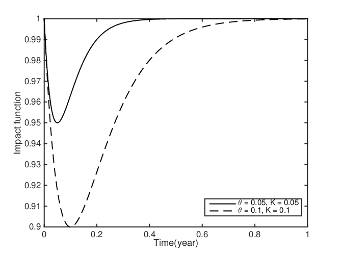
Figure 2 illustrates the impact function (2.4) with K=0.1K=0.1 and two different realized values of Θ\Theta. Clearly the shape of the impact function with Θ=0.05\Theta=0.05 is steeper than with Θ=0.1\Theta=0.1. We note that for each fixed scenario ω\omega, the function gg attains its minimum value 1−K⁡(ω)1-K(\omega) at t=Θ⁡(ω)t=\Theta(\omega). Also, we observe that the function gg first declines from 11 and then rises back and converges to 11, which characterizes the market impact of liquidation with time evolution. For realized values K=0.1K=0.1 and Θ=0.1\Theta=0.1 it would take 0.1 year, which is approximately 25 trading days, for the asset price to reach the minimum value (1−K)∗S0(1-K)*S_{0} after liquidation occurs. The market impact in the first trading day after liquidation is 1−g⁡(1250,0.1,0.1)≈1%1-g(\frac{1}{250};0.1,0.1)\approx 1\%. Therefore, the parameter Θ\Theta needs to be small to more accurately reflect the impact of disorderly liquidation. In Section 6 we present some numerical results which use a rather large Θ\Theta that guarantees better accuracy of the numerical results, but these could be improved by applying other numerical techniques for smaller values of Θ\Theta.

Refer to caption
Figure 1: Impact function with 2 parameters
Refer to caption
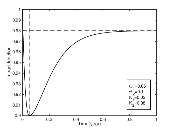
Figure 2: Impact function with 4 parameters
Remark 2.1.

It is natural to consider a jump effect for the price impact of liquidation. In our model, by (2.3), the price before and just after liquidation satisfies the relation StI​(t)=StS_{t}^{I}(t)=S_{t}. However, we can approximate downward jumps of asset prices after liquidation by choosing small values of Θ\Theta in the smooth function gg. Further, our model allows us to consider the situation that liquidation by the large trader may have no long-term informational content. The temporary impact on the market price decays as liquidity providers return to the market and other market participants realize that there may be no information about the fundamental value of the risky asset conveyed by the hedge fund’s disorderly liquidation.

A possible extension is to consider a modified impact function with additional parameters and flexibility. For example, let

g⁡(t,Θ1,Θ2,K1,K2)={1−(K1+K2)​tΘ1​e1−tΘ10≤t<Θ1,1−K1−K2​(t+Θ2−Θ1)Θ2​e1−t+Θ2−Θ1Θ2Θ1≤t.g(t;\Theta_{1},\Theta_{2},K_{1},K_{2})=\begin{cases}1-\frac{(K_{1}+K_{2})t}{\Theta_{1}}e^{1-\frac{t}{\Theta_{1}}}&0\leq t<\Theta_{1},\\ 1-K_{1}-\frac{K_{2}(t+\Theta_{2}-\Theta_{1})}{\Theta_{2}}e^{1-\frac{t+\Theta_{2}-\Theta_{1}}{\Theta_{2}}}&\Theta_{1}\leq t.\end{cases} (2.5)

The impact function given by (2.5) incorporates both permanent and temporary market impacts with K1K_{1} and K2K_{2} controlling the magnitude of permanent and temporary market impacts respectively. The parameters Θ1\Theta_{1} and Θ2\Theta_{2} determine both the deviation and reversal speed (see Figure 2). Moreover, at long-term time scale, the impact function can come back to a different level other than 11. For simplicity, we will use the impact function given by (2.4) in this paper and suppose the parameters Θ\Theta and KK to be random variables.

Considering the market price of the asset to be equal to the fundamental value before the liquidation time τ\tau and to be the impacted asset price after liquidation, we have that the market price is given as

StM=1{0≤t<τ∧T}St+1{τ∧T≤t≤T}StI(τ)S^{M}_{t}=1_{\{0\leq t<\tau\wedge T\}}S_{t}+1_{\{\tau\wedge T\leq t\leq T\}}S^{I}_{t}(\tau)

where StS_{t} and StI​(τ)S^{I}_{t}(\tau) are given by (2.1) and (2.3) respectively. Moreover, for any u≥0u\geq 0, the dynamics of the process StI​(u)S^{I}_{t}(u) satisfies the SDE

d​StI​(u)=StI​(u)​(μtI​(u,Θ,K)​d​t+σ​d​Wt),u≤t≤TdS_{t}^{I}(u)=S_{t}^{I}(u)\left(\mu^{I}_{t}(u,\Theta,K)dt+\sigma dW_{t}\right),\quad u\leq t\leq T (2.6)

where

μtI​(u,Θ,K)=g′​(t−u,Θ,K)g⁡(t−u,Θ,K)+μ.\mu^{I}_{t}(u,\Theta,K)=\frac{g^{\prime}(t-u;\Theta,K)}{g(t-u;\Theta,K)}+\mu. (2.7)
Remark 2.2.

The process (StI​(u),t≥u)(S_{t}^{I}(u),t\geq u) is adapted with respect to the filtration 𝔽∨σ⁡(Θ,K)\mathbb{F}\vee\sigma(\Theta,K) which is the initial enlargement of 𝔽\mathbb{F} by the random variables (Θ,K)(\Theta,K). As we suppose σ⁡(Θ,K)\sigma(\Theta,K) is independent of 𝔽∞\mathbb{F}_{\infty}, the (𝔽,ℙ)(\mathbb{F},\mathbb{P})-Brownian motion WW is also a (𝔽∨σ⁡(Θ,K),ℙ)(\mathbb{F}\vee\sigma(\Theta,K),\mathbb{P})-Brownian motion (see e.g. Jeanblanc et al. [17, Section 5.9].)

Thus the market price process of the risky asset, denoted as SM=(StM,t≥0)S^{M}=(S_{t}^{M},t\geq 0), satisfies the SDE

d​StM=StM​(μtM​(Θ,K)​d​t+σ​d​Wt)dS_{t}^{M}=S^{M}_{t}\left(\mu^{M}_{t}(\Theta,K)dt+\sigma dW_{t}\right) (2.8)

where

μtM(Θ,K)=1{0≤t<τ∧T}μ+1{τ∧T≤t≤T}μtI(τ,Θ,K).\mu^{M}_{t}(\Theta,K)=1_{\{0\leq t<\tau\wedge T\}}\mu+1_{\{\tau\wedge T\leq t\leq T\}}\mu^{I}_{t}(\tau,\Theta,K). (2.9)

We note that the market price admits a regime change at the liquidation time τ\tau, in particular on the drift term. We give an illustrative example as below.

Example 2.3.

Suppose that the fundamental value process (2.1) is given by the Black-Scholes model with parameters S0M=80,μ=0.07,σ=0.2,α=0.9,Θ=0.1,K=0.1S^{M}_{0}=80,\mu=0.07,\sigma=0.2,\alpha=0.9,\Theta=0.1,K=0.1. Figure 4 shows that liquidation triggers a downward jump of the drift term. Afterward the drift term first rises quickly and then declines gradually back to the original drift term. Correspondingly, Figure 4 shows the sample market price processes of the asset subject to liquidation impact compared with the fundamental value process.

Refer to caption
Figure 3: Drift μ\mu before and after liquidation
Refer to caption
Figure 4: Corresponding asset price SMS^{M}

2.2 The optimal investment problem

Our objective is to consider the optimal investment problem from the perspective of investors who trade in the market for the risky asset subject to price impact from disorderly liquidation of the hedge fund’s position. For simplicity we assume these agents may trade in the market for the risky asset without transaction costs. We consider fully informed investors, partially informed investors and uninformed investors. We suppose that all investors have access to the market price of the risky asset SMS^{M} but their knowledge of the liquidation and price impact are different. We further assume that all the investors know the values of the parameters μ\mu and σ\sigma.

Fully informed investors observe the market price and are assumed to have complete knowledge of the mechanism of liquidation and the price impact function. Hence they know, in mathematical terms, the liquidation trigger level α\alpha, the impact function gg, and the values of the random variables Θ\Theta and KK when liquidation occurs. Therefore, fully informed investors have complete knowledge of the dynamics of the market price process, together with the information of the price impact.

Partially informed investors are also able to observe the market price and know the liquidation trigger level α\alpha, therefore, the liquidation time τ\tau is also observable for them. However, partially informed investors do not have complete information about the price impact function. We suppose the partially informed investors know the functional form of the price impact function gg. However, we assume the partially informed investors only know the distributions of Θ\Theta and KK but not the realized value that is necessary to have full knowledge of the price impact of liquidation.

Uninformed investors are not aware of the liquidation trigger mechanism. They erroneously believe the market price process follows the Black-Scholes dynamics (2.1) without price impact. Considering uninformed investors allows us to quantify the value of information about the liquidation barrier and price impact, compared to a Merton-type investor.

We denote by 𝔽S=(ℱtS)t≥0\mathbb{F}^{S}=(\mathcal{F}^{S}_{t})_{t\geq 0} the natural filtration generated by the market price process SMS^{M}. Since the market price coincides with the fundamental value process SS before liquidation, the liquidation time τ\tau, which is an 𝔽\mathbb{F}-stopping time, is also an 𝔽S\mathbb{F}^{S}-stopping time. We summarize the knowledge of the various investors in the following assumption.

Assumption 2.4.

All investors observe the market price of the risky asset and know the values of the parameters μ\mu and σ\sigma. In addition certain market participants possess additional information:

  • (i)

    The observable information for fully informed investors is modeled by the filtration

    𝒢t(2)=ℱtS∨σ⁡(Θ,K)=ℱt∨σ⁡(Θ,K),\mathcal{G}^{(2)}_{t}=\mathcal{F}^{S}_{t}\vee\sigma(\Theta,K)=\mathcal{F}_{t}\vee\sigma(\Theta,K),

    they further know the liquidation barrier α\alpha, as well as the form of the impact function gg.

  • (ii)

    The observable information for partially informed investors is modeled by the filtration

    𝒢t(1)=ℱtS,\mathcal{G}^{(1)}_{t}=\mathcal{F}^{S}_{t},

    they further know the liquidation barrier α\alpha, the form of the impact function gg, and the distribution of (Θ,K)(\Theta,K).

  • (iii)

    To compare with the above two types of insiders, we consider uninformed investors whose observable information is modeled by the filtration 𝒢t(0)=ℱtS\mathcal{G}^{(0)}_{t}=\mathcal{F}^{S}_{t}. They have no information about the liquidation mechanism. Further, they do not update their knowledge of the drift process after τ\tau and act as Merton-type investors, erroneously considering Black-Scholes dynamics with constant μ\mu over the entire period [0,T][0,T].

Remark 2.5.

The common information to three types investors are represented by the "public" filtration 𝔽S\mathbb{F}^{S} since the market price of the risky asset is observable to all investors. Assumption 2.4 implies that partially informed investors know the the law of μtM​(Θ,K)\mu^{M}_{t}(\Theta,K). This is similar to the weak information case of Baudoin [8].

The essential differences among these three types of investors lie in their knowledge on the drift term μM​(Θ,K)\mu^{M}(\Theta,K) defined in (2.7). Fully informed investors are able to completely observe the drift term. Partially informed investors partially observe the drift term, corresponding to the case of partial observations considered by Karatzas and Zhao [19]. Partially informed investors may obtain an estimate of the drift term which is adapted to their observation process using filtering theory. Uninformed investors do not have any information about the liquidation mechanism and market impact which causes them to erroneously specify the drift term as μ\mu. That is, uninformed investors believe that the market prices follow the Black-Scholes dynamics (2.1). If the uninformed investor treated the drift of (2.1) as an unobservable process he could perhaps apply filtering theory to improve his investment decisions even without knowing anything about the liquidation mechanism or market impact function. However, in this paper we shall only consider the case of Assumption 2.4, that is of uninformed investors who estimate the drift at the beginning of the period and do not update it, since from their own view point no liquidation event happened during the period [0,T][0,T]. The uninformed investors are mainly considered as a benchmark for comparison with the Merton model.

We shall study the portfolio optimization problem for three types of investors in the remainder of this paper under logarithmic and power utility.

3 Fully informed investors

Fully informed investors choose their trading strategy to adjust the portfolio of assets according to their information accessibility. As discussed in Section 2 fully informed investors know the realized values of the random variables Θ\Theta and KK. The investment strategy is characterized by a 𝔾(2)\mathbb{G}^{(2)}-predictable process π(2)\pi^{(2)} which represents the proportion of wealth invested in the risky asset. The admissible strategy set 𝒜(2)\mathcal{A}^{(2)} is a collection of π(2)\pi^{(2)} such that, for any (θ,k)∈(0,+∞)×(0,1)(\theta,k)\in(0,+\infty)\times(0,1),

∫0T|πt(2)​μtM​(θ,k)|​𝑑t+∫0T|πt(2)​σ|2​𝑑t<∞.\int_{0}^{T}|\pi^{(2)}_{t}\mu^{M}_{t}(\theta,k)|dt+\int_{0}^{T}|\pi^{(2)}_{t}\sigma|^{2}dt<\infty. (3.1)

The risk aversion of the investors is modeled by classic utility functions UU defined on (0,∞)(0,\infty) that are strictly increasing, strictly concave, with continuous derivative U′​(x)U^{\prime}(x) on (0,∞)(0,\infty), and satisfying

limx→0+U′​(x)=+∞limx→∞U′​(x)=0.\lim_{x\rightarrow 0^{+}}U^{\prime}(x)=+\infty\quad\quad\lim_{x\rightarrow\infty}U^{\prime}(x)=0.

We define the 𝔾(2)\mathbb{G}^{(2)}-martingale measure ℚ\mathbb{Q} by the likelihood process

Lt:=d​ℚd​ℙ|𝒢t(2)=exp{−∫0tμvM​(Θ,K)σdWv−∫0t(μvM​(Θ,K))22​σ2dv}.L_{t}:=\left.\frac{d\mathbb{Q}}{d\mathbb{P}}\right|_{\mathcal{G}^{(2)}_{t}}=\exp\left\{-\int_{0}^{t}\frac{\mu^{M}_{v}(\Theta,K)}{\sigma}dW_{v}-\int_{0}^{t}\frac{\left(\mu^{M}_{v}(\Theta,K)\right)^{2}}{2\sigma^{2}}dv\right\}. (3.2)

As mentioned in Remark 2.2, WW is a (𝔾(2),ℙ)(\mathbb{G}^{(2)},\mathbb{P})-Brownian motion. By Girsanov’s theorem, the process WℚW^{\mathbb{Q}} defined as

Wtℚ=Wt+∫0tμvM​(Θ,K)σ​𝑑vW^{\mathbb{Q}}_{t}=W_{t}+\int_{0}^{t}\frac{\mu^{M}_{v}(\Theta,K)}{\sigma}dv (3.3)

is an (𝔾(2),ℚ)(\mathbb{G}^{(2)},\mathbb{Q})-Brownian motion and the dynamics of the asset price SMS^{M} under ℚ\mathbb{Q} may be written as

d​StM=StM​σ​d​Wtℚ.dS_{t}^{M}=S^{M}_{t}\sigma dW_{t}^{\mathbb{Q}}. (3.4)

By taking a strategy π2∈𝒜(2)\pi^{2}\in\mathcal{A}^{(2)}, the wealth process with initial endowment X0∈𝒢0(2)X_{0}\in\mathcal{G}^{(2)}_{0} evolves as

d​Xt(2)=Xt(2)​πt(2)​(μtM​(Θ,K)​d​t+σ​d​Wt),0≤t≤TdX_{t}^{(2)}=X_{t}^{(2)}\pi_{t}^{(2)}(\mu^{M}_{t}(\Theta,K)dt+\sigma dW_{t}),\quad\quad 0\leq t\leq T (3.5)

that is

Xt(2)=X0+∫0Tπv(2)​σ​SvM​d​Wvℚ.X^{(2)}_{t}=X_{0}+\int_{0}^{T}\pi^{(2)}_{v}\sigma S^{M}_{v}dW^{\mathbb{Q}}_{v}. (3.6)

The fully informed investor’s objective is to maximize her expected utility of terminal wealth

V0(2):=supπ(2)∈𝒜(2)𝔼⁡[U⁡(XT(2))]V^{(2)}_{0}:=\sup_{\pi^{(2)}\in\mathcal{A}^{(2)}}\mathbb{E}\left[U\left(X^{(2)}_{T}\right)\right] (3.7)

or

V0(2)​(Θ,K):=ess​supπ(2)​(Θ,K)∈𝒜(2)⁡𝔼​[U⁡(XT(2))|𝒢0(2)]V^{(2)}_{0}(\Theta,K):=\esssup_{\pi^{(2)}(\Theta,K)\in\mathcal{A}^{(2)}}\mathbb{E}\left[U\left(X^{(2)}_{T}\right)|\mathcal{G}^{(2)}_{0}\right] (3.8)

where 𝒢0(2)=σ⁡(Θ,K)\mathcal{G}^{(2)}_{0}=\sigma(\Theta,K). The link between the optimization problems (3.7) and (3.8) is given by Amendinger et al. [5]; if the supremum in (3.8) is attained by some strategy in 𝒜(2)\mathcal{A}^{(2)}, then the ω\omega-wise optimum is also a solution to (3.7).

As (Θ,K)(\Theta,K) is independent11 1 This assumption can be relaxed into a density Jacod hypothesis, using then the result of Amendinger [3, Proposition 4.6] for a martingale representation theorem. of 𝔽\mathbb{F}, a martingale representation theorem holds for (𝔾(2),ℚ)(\mathbb{G}^{(2)},\mathbb{Q})-local martingale, thus we adopt the standard "martingale approach" (see Karatzas and Shreve [18]) to solve the utility optimization problem (3.8). We may consider the following static optimization problem

supXT(2)∈𝒱𝔼⁡[U⁡(XT(2))|𝒢0(2)]\sup_{X^{(2)}_{T}\in\mathcal{V}}\mathbb{E}\left[U\left(X^{(2)}_{T}\right)|\mathcal{G}^{(2)}_{0}\right] (3.9)

where 𝒱={XT(2)|XT(2)=X0+∫0Tπv(2)σSvMdWvℚ,π(2)∈𝒜(2)}\mathcal{V}=\left\{X^{(2)}_{T}\left|X^{(2)}_{T}=X_{0}+\int_{0}^{T}\pi^{(2)}_{v}\sigma S^{M}_{v}dW^{\mathbb{Q}}_{v}\right.,\penalty\ \pi^{(2)}\in\mathcal{A}^{(2)}\right\}. The optimization problem (3.9) can be solved by using the method of Lagrange multipliers (see Amendinger et al. [5, Proposition 4.5]). The optimal terminal wealth X^T(2)\hat{X}^{(2)}_{T} is given by

X^T(2)=I⁡(Λ​LT),\hat{X}^{(2)}_{T}=I(\Lambda L_{T}), (3.10)

where I=(U′)−1I=(U^{\prime})^{-1} and the 𝒢0(2)\mathcal{G}^{(2)}_{0}-measurable random variable Λ\Lambda is determined by

𝔼ℚ[I(ΛLT)|𝒢0(2)]=X0.\mathbb{E}^{\mathbb{Q}}\left[\left.I(\Lambda L_{T})\right|\mathcal{G}^{(2)}_{0}\right]=X_{0}. (3.11)

In order to find the optimal strategy π^(2)\hat{\pi}^{(2)} one should provide the dynamics of the optimal wealth process

X^t(2)=𝔼ℚ​[X^T(2)|𝒢t(2)].\hat{X}^{(2)}_{t}=\mathbb{E}^{\mathbb{Q}}\left[\hat{X}^{(2)}_{T}|\mathcal{G}^{(2)}_{t}\right]. (3.12)

Since (Xt(2))t∈[0,T](X^{(2)}_{t})_{t\in[0,T]} is a (𝔾(2),ℚ)(\mathbb{G}^{(2)},\mathbb{Q})-martingale, there exists a 𝔾(2)\mathbb{G}^{(2)}-adapted process JJ such that

X^t(2)=𝔼ℚ[X^T(2)|𝒢0(2)]+∫0tJvdWvℚ.\hat{X}^{(2)}_{t}=\mathbb{E}^{\mathbb{Q}}[\left.\hat{X}^{(2)}_{T}\right|\mathcal{G}^{(2)}_{0}]+\int_{0}^{t}J_{v}dW^{\mathbb{Q}}_{v}. (3.13)

Substituting (3.11) into (3.13) we have

X^t(2)=X0+∫0tJv​d​Wvℚ.\hat{X}^{(2)}_{t}=X_{0}+\int_{0}^{t}J_{v}dW^{\mathbb{Q}}_{v}. (3.14)

Comparing (3.6) with (3.14), we obtain the optimal strategy

π^t(2)=Jtσ​X^t(2).\hat{\pi}^{(2)}_{t}=\frac{J_{t}}{\sigma\hat{X}^{(2)}_{t}}. (3.15)

Notice that the optimal strategy (π^t(2))t∈[0,T](\hat{\pi}^{(2)}_{t})_{t\in[0,T]} involves the process JJ which is implicitly determined by the martingale representation as in (3.13). To obtain an explicit expression for the optimal strategy, we will consider power and logarithmic utilities in the following subsections.

3.1 Power utility

We first consider the power utility U⁡(x)=xppU(x)=\frac{x^{p}}{p}, 0<p<10<p<1. Using the fact that I⁡(x)=xp−1I(x)=x^{p-1} and by (3.10)-(3.11) we obtain the optimal terminal wealth

X^T(2)=X0𝔼⁡[(LT)pp−1]​(LT)1p−1\hat{X}^{(2)}_{T}=\frac{X_{0}}{\mathbb{E}\left[\left(L_{T}\right)^{\frac{p}{p-1}}\right]}\left(L_{T}\right)^{\frac{1}{p-1}} (3.16)

where LTL_{T} is given by (3.2). The following proposition gives then the optimal expected utility as well as the optimal strategy:

Proposition 3.1.

For power utility U⁡(x)=xppU(x)=\frac{x^{p}}{p}, 0<p<10<p<1, the optimal expected utility is

V0(2)​(Θ,K)=(X0)pp​(𝔼⁡[(LT)pp−1])1−pV^{(2)}_{0}(\Theta,K)=\frac{(X_{0})^{p}}{p}\left(\mathbb{E}\left[\left(L_{T}\right)^{\frac{p}{p-1}}\right]\right)^{1-p} (3.17)

and the optimal strategy is given by

π^t(2)=1{0≤t<τ∧T}π^t(2,b)+1{τ∧T≤t≤T}π^t(2,a),t∈[0,T]\hat{\pi}_{t}^{(2)}=1_{\{0\leq t<\tau\wedge T\}}\hat{\pi}^{(2,b)}_{t}+1_{\{\tau\wedge T\leq t\leq T\}}\hat{\pi}_{t}^{(2,a)},\quad t\in[0,T] (3.18)

where

π^t(2,b)\displaystyle\hat{\pi}^{(2,b)}_{t} =μ(1−p)​σ2+ZtHσ​Ht,t∈[[0,τ∧T[[,\displaystyle=\frac{\mu}{(1-p)\sigma^{2}}+\frac{Z^{H}_{t}}{\sigma H_{t}},\quad t\in[\![0,\tau\wedge T[\![, (3.19)
π^t(2,a)\displaystyle\hat{\pi}^{(2,a)}_{t} =μtI​(τ,Θ,K)(1−p)​σ2,t∈[[τ∧T,T]]\displaystyle=\frac{\mu_{t}^{I}(\tau,\Theta,K)}{(1-p)\sigma^{2}},\quad t\in[\![\tau\wedge T,T]\!] (3.20)

with (H,ZH)(H,Z^{H}) satisfying the following linear BSDE

Ht=1+∫tT(p​(μvM​(Θ,K))22​(1−p)2​σ2​Hv+p​μvM​(Θ,K)(1−p)​σ​ZvH)​𝑑v−∫tTZvH​d​Wv.H_{t}=1+\int_{t}^{T}\left(\frac{p\left(\mu^{M}_{v}(\Theta,K)\right)^{2}}{2(1-p)^{2}\sigma^{2}}H_{v}+\frac{p\mu^{M}_{v}(\Theta,K)}{(1-p)\sigma}Z^{H}_{v}\right)dv-\int_{t}^{T}Z^{H}_{v}dW_{v}. (3.21)
Proof.

Following Björk et al. [9] we find the explicit expression for the optimal strategy, by computing the dynamics of the optimal wealth process. Applying the abstract Bayes’ formula to (3.12), we obtain

X^t(2)=\displaystyle\hat{X}^{(2)}_{t}= 𝔼ℚ​[X^T(2)|𝒢t(2)]\displaystyle\mathbb{E}^{\mathbb{Q}}\left[\hat{X}^{(2)}_{T}|\mathcal{G}^{(2)}_{t}\right]
=\displaystyle= 1Lt​𝔼​[X^T(2)​LT|𝒢t(2)].\displaystyle\frac{1}{L_{t}}\mathbb{E}\left[\hat{X}^{(2)}_{T}L_{T}|\mathcal{G}^{(2)}_{t}\right]. (3.22)

Substituting (3.2) and (3.16) into (3.22) we have

X^t(2)=\displaystyle\hat{X}^{(2)}_{t}= X0𝔼⁡[(LT)pp−1]​Lt​𝔼​[(LT)pp−1|𝒢t(2)]\displaystyle\frac{X_{0}}{\mathbb{E}[(L_{T})^{\frac{p}{p-1}}]L_{t}}\mathbb{E}\left[(L_{T})^{\frac{p}{p-1}}|\mathcal{G}^{(2)}_{t}\right]
=\displaystyle= X0𝔼⁡[(LT)pp−1]​Lt​𝔼​[exp⁡{∫0Tp​μvM​(Θ,K)(1−p)​σ​d​Wv+∫0Tp​(μvM​(Θ,K))22​(1−p)​σ2​𝑑v}|𝒢t(2)]\displaystyle\frac{X_{0}}{\mathbb{E}[(L_{T})^{\frac{p}{p-1}}]L_{t}}\mathbb{E}\left[\exp\left\{\int_{0}^{T}\frac{p\mu^{M}_{v}(\Theta,K)}{(1-p)\sigma}dW_{v}+\int_{0}^{T}\frac{p\left(\mu^{M}_{v}(\Theta,K)\right)^{2}}{2(1-p)\sigma^{2}}dv\right\}|\mathcal{G}^{(2)}_{t}\right]
=\displaystyle= X0​(Lt)1p−1𝔼⁡[(LT)pp−1]​𝔼​[exp⁡{∫tTp​μvM​(Θ,K)(1−p)​σ​d​Wv+∫tTp​(μvM​(Θ,K))22​(1−p)​σ2​𝑑v}|𝒢t(2)]\displaystyle\frac{X_{0}(L_{t})^{\frac{1}{p-1}}}{\mathbb{E}[(L_{T})^{\frac{p}{p-1}}]}\mathbb{E}\left[\exp\left\{\int_{t}^{T}\frac{p\mu^{M}_{v}(\Theta,K)}{(1-p)\sigma}dW_{v}+\int_{t}^{T}\frac{p\left(\mu^{M}_{v}(\Theta,K)\right)^{2}}{2(1-p)\sigma^{2}}dv\right\}|\mathcal{G}^{(2)}_{t}\right] (3.23)

Defining

Ht:=𝔼⁡[exp⁡{∫tTp​μvM​(Θ,K)(1−p)​σ​d​Wv+∫tTp​(μvM​(Θ,K))22​(1−p)​σ2​𝑑v}|𝒢t(2)]H_{t}:=\mathbb{E}[\exp\left\{\int_{t}^{T}\frac{p\mu_{v}^{M}(\Theta,K)}{(1-p)\sigma}dW_{v}+\int_{t}^{T}\frac{p(\mu_{v}^{M}(\Theta,K))^{2}}{2(1-p)\sigma^{2}}dv\right\}|\mathcal{G}^{(2)}_{t}] (3.24)

the optimal wealth process writes as

X^t(2)=X0H0​(Lt)1p−1​Ht.\hat{X}^{(2)}_{t}=\frac{X_{0}}{H_{0}}(L_{t})^{\frac{1}{p-1}}H_{t}. (3.25)

In order to find the dynamics of (Ht)t∈[0,T](H_{t})_{t\in[0,T]}, we first remark that (Mt:=Ht​Dt)t∈[0,T](M_{t}:=H_{t}D_{t})_{t\in[0,T]} is a (𝔾(2),ℙ)(\mathbb{G}^{(2)},\mathbb{P})-martingale, where

Dt:=exp⁡{∫0tp​μvM​(Θ,K)(1−p)​σ​d​Wv+∫0tp​(μvM​(Θ,K))22​(1−p)​σ2​𝑑v}.D_{t}:=\exp\left\{\int_{0}^{t}\frac{p\mu_{v}^{M}(\Theta,K)}{(1-p)\sigma}dW_{v}+\int_{0}^{t}\frac{p(\mu_{v}^{M}(\Theta,K))^{2}}{2(1-p)\sigma^{2}}dv\right\}. (3.26)

By the martingale representation theorem there exists a 𝔾(2)\mathbb{G}^{(2)}-adapted process ZMZ^{M} such that

Mt=M0+∫0tMv​ZvM​d​Wv.M_{t}=M_{0}+\int_{0}^{t}M_{v}Z^{M}_{v}dW_{v}. (3.27)

From equation (3.26)

d⁡(1Dt)=(1Dt)​{(p2​(μtM​(Θ,K))22​(1−p)2​σ2−p​(μtM​(Θ,K))22​(1−p)​σ2)​d​t−p​μtM​(Θ,K)(1−p)​σ​d​Wt}d(\frac{1}{D_{t}})=(\frac{1}{D_{t}})\left\{\left(\frac{p^{2}(\mu_{t}^{M}(\Theta,K))^{2}}{2(1-p)^{2}\sigma^{2}}-\frac{p(\mu_{t}^{M}(\Theta,K))^{2}}{2(1-p)\sigma^{2}}\right)dt-\frac{p\mu_{t}^{M}(\Theta,K)}{(1-p)\sigma}dW_{t}\right\} (3.28)

which leads to the following dynamics for the process (Ht)t∈[0,T](H_{t})_{t\in[0,T]}

d​Ht=Ht​{(p2​(μtM​(Θ,K))22​(1−p)2​σ2−p​(μtM​(Θ,K))22​(1−p)​σ2−p​μtM​(Θ,K)(1−p)​σ​ZtM)​d​t+(ZtM−p​μtM​(Θ,K)(1−p)​σ)​d​Wt}.dH_{t}=H_{t}\left\{\left(\frac{p^{2}(\mu_{t}^{M}(\Theta,K))^{2}}{2(1-p)^{2}\sigma^{2}}-\frac{p(\mu_{t}^{M}(\Theta,K))^{2}}{2(1-p)\sigma^{2}}-\frac{p\mu_{t}^{M}(\Theta,K)}{(1-p)\sigma}Z^{M}_{t}\right)dt+\left(Z^{M}_{t}-\frac{p\mu_{t}^{M}(\Theta,K)}{(1-p)\sigma}\right)dW_{t}\right\}.

Denoting ZtH:=Ht​ZtM−p​μtM​(Θ,K)(1−p)​σZ^{H}_{t}:=H_{t}Z^{M}_{t}-\frac{p\mu_{t}^{M}(\Theta,K)}{(1-p)\sigma} and using the terminal condition HT=1H_{T}=1, (Ht)t∈[0,T](H_{t})_{t\in[0,T]} satisfies the following BSDE

Ht=1+∫tT(p​(μvM​(Θ,K))22​(1−p)2​σ2​Hv+p​μvM​(Θ,K)(1−p)​σ​ZvH)​𝑑v−∫tTZvH​d​Wv.H_{t}=1+\int_{t}^{T}\left(\frac{p(\mu_{v}^{M}(\Theta,K))^{2}}{2(1-p)^{2}\sigma^{2}}H_{v}+\frac{p\mu_{v}^{M}(\Theta,K)}{(1-p)\sigma}Z^{H}_{v}\right)dv-\int_{t}^{T}Z^{H}_{v}dW_{v}. (3.29)

Thus the dynamics of the optimal wealth process, using (3.25), are

d​X^t(2)=X^t(2)​((μtM​(Θ,K))2(1−p)​σ2+μtM​(Θ,K)​ZtHσ​Ht)​d​t+X^t(2)​(μtM​(Θ,K)(1−p)​σ+ZtHHt)​d​Wt.d\hat{X}^{(2)}_{t}=\hat{X}^{(2)}_{t}\left(\frac{\left(\mu_{t}^{M}(\Theta,K)\right)^{2}}{(1-p)\sigma^{2}}+\frac{\mu_{t}^{M}(\Theta,K)Z^{H}_{t}}{\sigma H_{t}}\right)dt+\hat{X}^{(2)}_{t}\left(\frac{\mu_{t}^{M}(\Theta,K)}{(1-p)\sigma}+\frac{Z^{H}_{t}}{H_{t}}\right)dW_{t}. (3.30)

that leads to the optimal strategy (by comparing (3.30) with (3.5))

π^t(2)=μtM​(Θ,K)(1−p)​σ2+ZtHσ​Ht.\hat{\pi}^{(2)}_{t}=\frac{\mu_{t}^{M}(\Theta,K)}{(1-p)\sigma^{2}}+\frac{Z^{H}_{t}}{\sigma H_{t}}. (3.31)

We decompose the time horizon [0,T][0,T] into two random time intervals [[0,τ∧T[[[\![0,\tau\wedge T[\![ and [[τ∧T,T]][\![\tau\wedge T,T]\!]. On the random interval [[τ∧T,T]][\![\tau\wedge T,T]\!], the fully informed investor observes the drift term μM\mu^{M} thus the BSDE (3.29) can be solved explicitly on [[τ∧T,T]][\![\tau\wedge T,T]\!]:

Ht\displaystyle H_{t} =exp⁡{∫tTp​(μvI​(τ,Θ,K))22​(1−p)2​σ2​𝑑v},\displaystyle=\exp\left\{\int_{t}^{T}\frac{p(\mu_{v}^{I}(\tau,\Theta,K))^{2}}{2(1-p)^{2}\sigma^{2}}dv\right\}, (3.32)
ZtH\displaystyle Z^{H}_{t} =0.\displaystyle=0. (3.33)

Recalling (2.9) and using (3.32)-(3.33) we may decompose the optimal strategy in (3.31) into two parts:

π^t(2)=1{0≤t<τ∧T}π^t(2,b)+1{τ∧T≤t≤T}π^t(2,a)(3.18)\hat{\pi}_{t}^{(2)}=1_{\{0\leq t<\tau\wedge T\}}\hat{\pi}^{(2,b)}_{t}+1_{\{\tau\wedge T\leq t\leq T\}}\hat{\pi}_{t}^{(2,a)}\quad(\ref{eq:optimal_strategy_power_fully_informed_decomposed})

where

π^t(2,b)\displaystyle\hat{\pi}^{(2,b)}_{t} =μ(1−p)​σ2+ZtHσ​Ht,t∈[[0,τ∧T[[,(3.19)\displaystyle=\frac{\mu}{(1-p)\sigma^{2}}+\frac{Z^{H}_{t}}{\sigma H_{t}},\quad t\in[\![0,\tau\wedge T[\![,\quad(\ref{eq:optimal_strategy_power_fully_informed_before_liquidation}) (3.34)
π^t(2,a)\displaystyle\hat{\pi}^{(2,a)}_{t} =μtI​(τ,Θ,K)(1−p)​σ2,t∈[[τ∧T,T]].(3.20)\displaystyle=\frac{\mu_{t}^{I}(\tau,\Theta,K)}{(1-p)\sigma^{2}},\quad t\in[\![\tau\wedge T,T]\!].\quad(\ref{eq:optimal_strategy_power_fully_informed_after_liquidation}) (3.35)

∎

The optimal strategy after liquidation in (3.20) is essentially a Merton-type strategy. The part before liquidation in (3.19) is the sum of a Merton strategy and an extra component22 2 This extra term is called ”hedging demand for parameter risk” by Björk [9]. which is determined by the solution of the BSDE (3.21). It is hard to obtain a closed-form solution for the BSDE (3.21), however, we may solve the BSDE (3.21) numerically which will be discussed in Section 6.

We next consider the case of logarithmic utility for the fully informed investor.

3.2 Logarithmic utility

In this section we consider the logarithmic utility U⁡(x)=ln⁡(x)U(x)=\ln(x). Using the fact that I⁡(x)=1xI(x)=\frac{1}{x} and by (3.10)-(3.11) we obtain the optimal terminal wealth

X^T(2)=X0LT\hat{X}^{(2)}_{T}=\frac{X_{0}}{L_{T}} (3.36)

where LTL_{T} is given by (3.2). The optimal expected utility is

V0(2)​(Θ,K)=ln⁡(X0)−𝔼⁡[ln⁡(LT)].V^{(2)}_{0}(\Theta,K)=\ln(X_{0})-\mathbb{E}\left[\ln(L_{T})\right].

Applying the abstract Bayes’ formula to (3.12) and using (3.36), we obtain

X^t(2)=\displaystyle\hat{X}^{(2)}_{t}= 𝔼ℚ​[X^T(2)|𝒢t(2)]\displaystyle\mathbb{E}^{\mathbb{Q}}\left[\hat{X}^{(2)}_{T}|\mathcal{G}^{(2)}_{t}\right]
=\displaystyle= 1Lt​𝔼​[X^T(2)​LT|𝒢t(2)]\displaystyle\frac{1}{L_{t}}\mathbb{E}\left[\hat{X}^{(2)}_{T}L_{T}|\mathcal{G}^{(2)}_{t}\right]
=\displaystyle= X0Lt\displaystyle\frac{X_{0}}{L_{t}} (3.37)

whose dynamics are given by

d​X^t(2)=(μtM​(Θ,K))22​σ2​d​t+μtM​(Θ,K)σ​d​Wt.d\hat{X}^{(2)}_{t}=\frac{\left(\mu^{M}_{t}(\Theta,K)\right)^{2}}{2\sigma^{2}}dt+\frac{\mu^{M}_{t}(\Theta,K)}{\sigma}dW_{t}. (3.38)

Comparing (3.38) with (3.5) we obtain the optimal strategy

π^t(2)=μtM​(Θ,K)σ2.\hat{\pi}^{(2)}_{t}=\frac{\mu_{t}^{M}(\Theta,K)}{\sigma^{2}}.

Recalling (2.9) we may decompose the optimal strategy into two parts

π^t(2)=1{0≤t<τ∧T}π^(2,b)t+1{τ∧T≤t≤T}π^t(2,a)\hat{\pi}_{t}^{(2)}=1_{\{0\leq t<\tau\wedge T\}}\hat{\pi}^{(2,b)}_{t}+1_{\{\tau\wedge T\leq t\leq T\}}\hat{\pi}_{t}^{(2,a)} (3.39)

where

π^t(2,b)\displaystyle\hat{\pi}^{(2,b)}_{t} =μσ2,t∈[[0,τ∧T[[,\displaystyle=\frac{\mu}{\sigma^{2}},\quad t\in[\![0,\tau\wedge T[\![, (3.40)
π^t(2,a)\displaystyle\hat{\pi}^{(2,a)}_{t} =μtI​(τ,Θ,K)σ2,t∈[[τ∧T,T]].\displaystyle=\frac{\mu^{I}_{t}(\tau,\Theta,K)}{\sigma^{2}},\quad t\in[\![\tau\wedge T,T]\!]. (3.41)

The optimal trading strategy for the fully informed investor is composed of two Merton strategies before and after-liquidation. Accordingly we decompose the optimal wealth process X^t(2)\hat{X}^{(2)}_{t} as

X^(2)t=1{0≤t<τ∧T}X^(2,b)t+1{τ∧T≤t≤T}X^(2,a)t\hat{X}^{(2)}_{t}=1_{\{0\leq t<\tau\wedge T\}}\hat{X}^{(2,b)}_{t}+1_{\{\tau\wedge T\leq t\leq T\}}\hat{X}^{(2,a)}_{t}

where X^(2,b)\hat{X}^{(2,b)} and X^(2,a)\hat{X}^{(2,a)} satisfy the following SDEs

d​X^t(2,b)\displaystyle d\hat{X}_{t}^{(2,b)} =X^t(2,b)​π^t(2,b)​(μt​d​t+σ​d​Wt),\displaystyle=\hat{X}_{t}^{(2,b)}\hat{\pi}^{(2,b)}_{t}(\mu_{t}dt+\sigma dW_{t}), t∈[[0,τ∧T[[,\displaystyle t\in[\![0,\tau\wedge T[\![, (3.42)
d​X^t(2,a)\displaystyle d\hat{X}_{t}^{(2,a)} =X^t(2,a)​π^t(2,a)​{μtI​(τ,Θ,K)​d​t+σ​d​Wt},\displaystyle=\hat{X}_{t}^{(2,a)}\hat{\pi}^{(2,a)}_{t}\left\{\mu^{I}_{t}(\tau,\Theta,K)dt+\sigma dW_{t}\right\}, t∈[[τ∧T,T]].\displaystyle t\in[\![\tau\wedge T,T]\!]. (3.43)

Then we decompose the expected utility of terminal wealth into two parts depending on if liquidation occurs before or after time TT:

V0(2)(Θ,K)=𝔼[1{τ>T}ln(X^T(2,b))|𝒢0(2)]+𝔼[1{τ≤T}ln(X^T(2,a))|𝒢0(2)].V^{(2)}_{0}(\Theta,K)=\mathbb{E}[1_{\{\tau>T\}}\ln(\hat{X}^{(2,b)}_{T})|\mathcal{G}_{0}^{(2)}]+\mathbb{E}[1_{\{\tau\leq T\}}\ln(\hat{X}^{(2,a)}_{T})|\mathcal{G}_{0}^{(2)}]. (3.44)

The two conditional expectations in (3.44) are calculated in Lemma A.1 and A.2 respectively. Combining those lemmas we obtain the following result.

Proposition 3.2.

The optimal log expected utility for fully informed investors is

V0(2)​(Θ,K)=\displaystyle V^{(2)}_{0}(\Theta,K)=
{𝒩⁡(−ln⁡ασ+(μσ−12​σ)​TT)−exp⁡(2​μσ2−ln⁡α)​𝒩​(ln⁡ασ+(μσ−12​σ)​TT)}×(ln⁡(X0)+12​(μ−μ2σ2)​T)\displaystyle\left\{\mathcal{N}\left(\frac{-\frac{\ln\alpha}{\sigma}+(\frac{\mu}{\sigma}-\frac{1}{2}\sigma)T}{\sqrt{T}}\right)-\exp\left(\frac{2\mu}{\sigma^{2}}-\ln\alpha\right)\mathcal{N}\left(\frac{\frac{\ln\alpha}{\sigma}+(\frac{\mu}{\sigma}-\frac{1}{2}\sigma)T}{\sqrt{T}}\right)\right\}\times\left(\ln(X_{0})+\frac{1}{2}(\mu-\frac{\mu^{2}}{\sigma^{2}})T\right)
+∫ln⁡ασ0∫y∞2​μ​x​(x−2​y)2​π​T3exp{(μσ−12σ)x−12(μσ−12σ)2T−12​T(2y−x)2}dxdy\displaystyle+\int_{\frac{\ln\alpha}{\sigma}}^{0}\int_{y}^{\infty}\frac{2\mu x(x-2y)}{\sqrt{2\pi T^{3}}}\exp\left\{(\frac{\mu}{\sigma}-\frac{1}{2}\sigma)x-\frac{1}{2}(\frac{\mu}{\sigma}-\frac{1}{2}\sigma)^{2}T-\frac{1}{2T}(2y-x)^{2}\right\}dxdy
−ln⁡ασ∫0T12​π​t3exp{−12​t(ln⁡ασ−(μσ−12σ)t)2}h(2)(t,Θ,K)dt\displaystyle-\frac{\ln\alpha}{\sigma}\int_{0}^{T}\frac{1}{\sqrt{2\pi t^{3}}}\exp\left\{-\frac{1}{2t}\left(\frac{\ln\alpha}{\sigma}-(\frac{\mu}{\sigma}-\frac{1}{2}\sigma)t\right)^{2}\right\}h^{(2)}(t,\Theta,K)dt

where

h(2)​(t,θ,k):=ln⁡X0+μ​ln⁡ασ2+μ2​t−μ22​σ2​t+∫tT(μvI​(t,θ,k))22​σ2​𝑑v.h^{(2)}(t;\theta,k):=\ln X_{0}+\frac{\mu\ln\alpha}{\sigma^{2}}+\frac{\mu}{2}t-\frac{\mu^{2}}{2\sigma^{2}}t+\int_{t}^{T}\frac{\left(\mu^{I}_{v}(t,\theta,k)\right)^{2}}{2\sigma^{2}}dv.

In the next section we consider the optimization problem for the partially informed investors.

4 Partially informed investors

The portfolio strategy for partially informed investors is supposed to be 𝔾(1)\mathbb{G}^{(1)}-adapted and denoted by π(1)=(πt(1),0≤t≤T)\pi^{(1)}=(\pi^{(1)}_{t},0\leq t\leq T). The wealth process evolves as

d​Xt(1)=Xt(1)​πt(1)​(μtM​(Θ,K)​d​t+σ​d​Wt),0≤t≤T.dX_{t}^{(1)}=X_{t}^{(1)}\pi_{t}^{(1)}(\mu^{M}_{t}(\Theta,K)dt+\sigma dW_{t}),\quad\quad 0\leq t\leq T. (4.1)

Similar to (3.1), the admissible strategy set 𝒜(1)\mathcal{A}^{(1)} is a collection of π(1)\pi^{(1)} such that, for any (θ,k)∈(0,+∞)×(0,1)(\theta,k)\in(0,+\infty)\times(0,1),

∫0T|πt(1)​μtM​(θ,k)|​𝑑t+∫0T|πt(1)​σ|2​𝑑t<∞.\int_{0}^{T}|\pi^{(1)}_{t}\mu^{M}_{t}(\theta,k)|dt+\int_{0}^{T}|\pi^{(1)}_{t}\sigma|^{2}dt<\infty. (4.2)

The portfolio optimization problem for partially informed investors is

V0(1)=supπ(1)∈𝒜(1)𝔼⁡[U⁡(XT(1))].V^{(1)}_{0}=\sup_{\pi^{(1)}\in\mathcal{A}^{(1)}}\mathbb{E}\left[U\left(X^{(1)}_{T}\right)\right]. (4.3)

Note that the optimization problem (4.1)-(4.3) is the case of partial observations since the drift term in (4.1) is not 𝔾(1)\mathbb{G}^{(1)}-adapted.

Following Karatzas and Zhao [19] we first reduce the optimization problem of partial observation to the case of complete observation. Recall that the probability measure ℚ\mathbb{Q} is defined as

d​ℚd​ℙ|𝒢T(2)=LT.\left.\frac{d\mathbb{Q}}{d\mathbb{P}}\right|_{\mathcal{G}^{(2)}_{T}}=L_{T}. (4.4)

with the density process

Lt=exp{−∫0tμvM​(Θ,K)σdWv−∫0t(μvM​(Θ,K))22​σ2dv}L_{t}=\exp\left\{-\int_{0}^{t}\frac{\mu^{M}_{v}(\Theta,K)}{\sigma}dW_{v}-\int_{0}^{t}\frac{\left(\mu^{M}_{v}(\Theta,K)\right)^{2}}{2\sigma^{2}}dv\right\} (4.5)

being a (𝔾(2),ℙ)(\mathbb{G}^{(2)},\mathbb{P})-martingale.

We next define the filtered estimate of the drift μtM​(Θ,K)\mu^{M}_{t}(\Theta,K), based on the observation of the market price, by

μ¯tM=𝔼⁡[μtM​(Θ,K)|𝒢t(1)].\bar{\mu}^{M}_{t}=\mathbb{E}\left[\mu^{M}_{t}(\Theta,K)|\mathcal{G}^{(1)}_{t}\right]. (4.6)

We define the innovations process W~\tilde{W} by

d​W~t=d​Wt+μtM​(Θ,K)−μ¯tMσ​d​t,0≤t≤T.d\tilde{W}_{t}=dW_{t}+\frac{\mu^{M}_{t}(\Theta,K)-\bar{\mu}^{M}_{t}}{\sigma}dt,\quad 0\leq t\leq T. (4.7)

By Björk et al. [9, Lemma 4.1] we know W~\tilde{W} is a standard (𝔾(1),ℙ)(\mathbb{G}^{(1)},\mathbb{P})-Brownian motion. Then we may rewrite (2.8) as

d​StM=StM​(μ¯tM​d​t+σ​d​W~t).dS_{t}^{M}=S^{M}_{t}\left(\bar{\mu}^{M}_{t}dt+\sigma d\tilde{W}_{t}\right). (4.8)

and the wealth process X(1)X^{(1)} as

d​Xt(1)=Xt(1)​πt(1)​(μ¯tM​d​t+σ​d​W~t),0≤t≤TdX_{t}^{(1)}=X_{t}^{(1)}\pi_{t}^{(1)}(\bar{\mu}^{M}_{t}dt+\sigma d\tilde{W}_{t}),\quad\quad 0\leq t\leq T (4.9)

with initial wealth x0∈]0,+∞[x_{0}\in]0,+\infty[. Now the dynamics of the wealth process X(1)X^{(1)} is within the framework of a full observation model since μ¯M\bar{\mu}^{M} is 𝔾(1)\mathbb{G}^{(1)}-adapted.

Similar to the case of fully informed investors, the optimization problem (4.3) can be solved by the martingale approach.

Proposition 4.1.

(i)The optimal terminal wealth of a partially informed investors, with utility function UU and I=(U′)−1I=(U^{\prime})^{-1} is given by

X^T(1)=I⁡(λ​L¯T).\hat{X}^{(1)}_{T}=I(\lambda\bar{L}_{T}).

The Lagrange multiplier λ\lambda is determined by the budget constraint

𝔼⁡[I⁡(λ​L¯T)​L¯T]=x0\mathbb{E}\left[I(\lambda\bar{L}_{T})\bar{L}_{T}\right]=x_{0} (4.10)

and L¯T\bar{L}_{T} is the density of the risk neutral probability measure for the filtration 𝔾(1)\mathbb{G}^{(1)}

L¯t=exp{−∫0tμ¯vMσdW~v−∫0t(μ¯vM)22​σ2dv}\bar{L}_{t}=\exp\left\{-\int_{0}^{t}\frac{\bar{\mu}^{M}_{v}}{\sigma}d\tilde{W}_{v}-\int_{0}^{t}\frac{\left(\bar{\mu}^{M}_{v}\right)^{2}}{2\sigma^{2}}dv\right\} (4.11)

with μ¯tM=𝔼⁡[μtM​(Θ,K)|𝒢t(1)]\bar{\mu}^{M}_{t}=\mathbb{E}\left[\mu^{M}_{t}(\Theta,K)|\mathcal{G}^{(1)}_{t}\right]

(ii) The filtered drift estimate μ¯M\bar{\mu}^{M} can be computed as

μ¯tM={μ,t∈[[0,τ∧T[[∫0∞∫01{μtM​(θ,k)​exp⁡{∫0tμvM​(θ,k)σ​d​Wvℚ−∫0t(μvM​(θ,k))22​σ2​𝑑v}}​φ​(θ,k)​𝑑θ​𝑑k∫0∞∫01{exp⁡{∫0tμvM​(θ,k)σ​d​Wvℚ−∫0t(μvM​(θ,k))22​σ2​𝑑v}}​φ​(θ,k)​𝑑θ​𝑑k,t∈[[τ∧T,T]].\bar{\mu}^{M}_{t}=\begin{cases}\mu,&t\in[\![0,\tau\wedge T[\![\\ \frac{\int_{0}^{\infty}\int_{0}^{1}\left\{\mu^{M}_{t}(\theta,k)\exp\left\{\int_{0}^{t}\frac{\mu^{M}_{v}(\theta,k)}{\sigma}dW^{\mathbb{Q}}_{v}-\int_{0}^{t}\frac{\left(\mu^{M}_{v}(\theta,k)\right)^{2}}{2\sigma^{2}}dv\right\}\right\}\varphi(\theta,k)d\theta dk}{\int_{0}^{\infty}\int_{0}^{1}\left\{\exp\left\{\int_{0}^{t}\frac{\mu^{M}_{v}(\theta,k)}{\sigma}dW^{\mathbb{Q}}_{v}-\int_{0}^{t}\frac{\left(\mu^{M}_{v}(\theta,k)\right)^{2}}{2\sigma^{2}}dv\right\}\right\}\varphi(\theta,k)d\theta dk},&t\in[\![\tau\wedge T,T]\!].\end{cases} (4.12)
Proof.

(i) We define the process L¯t=𝔼ℚ​[Lt|𝒢t(1)]\bar{L}_{t}=\mathbb{E}^{\mathbb{Q}}[L_{t}|\mathcal{G}^{(1)}_{t}]. By rewriting LtL_{t} in (4.5) as

Lt=exp{−∫0tμvM​(Θ,K)σdWvℚ+∫0t(μvM​(Θ,K))22​σ2dv},L_{t}=\exp\left\{-\int_{0}^{t}\frac{\mu^{M}_{v}(\Theta,K)}{\sigma}d{W}^{\mathbb{Q}}_{v}+\int_{0}^{t}\frac{\left(\mu^{M}_{v}(\Theta,K)\right)^{2}}{2\sigma^{2}}dv\right\}, (4.13)

we compute

L¯t=exp{−∫0tμ¯vMσdWvℚ+∫0t(μ¯vM)22​σ2dv}\bar{L}_{t}=\exp\left\{-\int_{0}^{t}\frac{\bar{\mu}^{M}_{v}}{\sigma}dW^{\mathbb{Q}}_{v}+\int_{0}^{t}\frac{\left(\bar{\mu}^{M}_{v}\right)^{2}}{2\sigma^{2}}dv\right\} (4.14)

Combining (4.18) and (4.7) we have

d​Wtℚ=d​W~t+μ¯tMσ​d​t.dW^{\mathbb{Q}}_{t}=d\tilde{W}_{t}+\frac{\bar{\mu}^{M}_{t}}{\sigma}dt. (4.15)

Substituting (4.15) into (4.14) we find

L¯t=exp{−∫0tμ¯vMσdW~v−∫0t(μ¯vM)22​σ2dv}.\bar{L}_{t}=\exp\left\{-\int_{0}^{t}\frac{\bar{\mu}^{M}_{v}}{\sigma}d\tilde{W}_{v}-\int_{0}^{t}\frac{\left(\bar{\mu}^{M}_{v}\right)^{2}}{2\sigma^{2}}dv\right\}. (4.16)

Since L¯t\bar{L}_{t} is a (𝔾(1),ℙ)(\mathbb{G}^{(1)},\mathbb{P})-martingale, we define the the risk neutral probability measure ℚ~\tilde{\mathbb{Q}} by

d​ℚ~d​ℙ|𝒢t(1)=L¯t.\left.\frac{d\tilde{\mathbb{Q}}}{d\mathbb{P}}\right|_{\mathcal{G}^{(1)}_{t}}=\bar{L}_{t}. (4.17)

By the fact that W~\tilde{W} is a (𝔾(1),ℙ)(\mathbb{G}^{(1)},\mathbb{P})-Brownian motion and the Girsanov’s theorem, the process Wℚ~W^{\tilde{\mathbb{Q}}} defined as

Wtℚ~=W~t+∫0tμ¯vMσ​𝑑v,0≤t≤TW^{\tilde{\mathbb{Q}}}_{t}=\tilde{W}_{t}+\int_{0}^{t}\frac{\bar{\mu}^{M}_{v}}{\sigma}dv,\quad 0\leq t\leq T (4.18)

is a (𝔾(1),ℚ~)(\mathbb{G}^{(1)},\tilde{\mathbb{Q}})-Brownian motion.

Following the same procedure as in Section 3 we find the optimal terminal wealth X^T(1)\hat{X}^{(1)}_{T} given by

X^T(1)=I⁡(λ​L¯T),\hat{X}^{(1)}_{T}=I(\lambda\bar{L}_{T}), (4.19)

where I=(U′)−1I=(U^{\prime})^{-1} and the Lagrange multiplier λ\lambda is determined by

𝔼⁡[I⁡(λ​L¯T)​L¯T]=x0.\mathbb{E}\left[I(\lambda\bar{L}_{T})\bar{L}_{T}\right]=x_{0}. (4.20)

(ii) Recall that

1Lt=d​ℙd​ℚ|𝒢t(2)=exp⁡{∫0tμvM​(Θ,K)σ​d​Wvℚ−∫0t(μvM​(Θ,K))22​σ2​𝑑v}\frac{1}{L_{t}}=\left.\frac{d\mathbb{P}}{d\mathbb{Q}}\right|_{\mathcal{G}^{(2)}_{t}}=\exp\left\{\int_{0}^{t}\frac{\mu^{M}_{v}(\Theta,K)}{\sigma}dW^{\mathbb{Q}}_{v}-\int_{0}^{t}\frac{\left(\mu^{M}_{v}(\Theta,K)\right)^{2}}{2\sigma^{2}}dv\right\} (4.21)

is (𝔾(2),ℚ)(\mathbb{G}^{(2)},\mathbb{Q})-martingale. By the Kallianpur-Striebel formula, which is related to Bayes formula, we have

μ¯tM=\displaystyle\bar{\mu}^{M}_{t}= 𝔼⁡[μtM​(Θ,K)|𝒢t(1)]\displaystyle\mathbb{E}\left[\mu^{M}_{t}(\Theta,K)|\mathcal{G}^{(1)}_{t}\right]
=\displaystyle= 𝔼ℚ​[μtM​(Θ,K)​LT|𝒢t(1)]𝔼ℚ​[Lt|𝒢t(1)]\displaystyle\frac{\mathbb{E}^{\mathbb{Q}}\left[\mu^{M}_{t}(\Theta,K)L_{T}|\mathcal{G}^{(1)}_{t}\right]}{\mathbb{E}^{\mathbb{Q}}[L_{t}|\mathcal{G}^{(1)}_{t}]}
=\displaystyle= 𝔼ℚ​[𝔼ℚ​[μtM​(Θ,K)​LT|𝒢t(2)]|𝒢t(1)]𝔼ℚ​[Lt|𝒢t(1)]\displaystyle\frac{\mathbb{E}^{\mathbb{Q}}\left[\mathbb{E}^{\mathbb{Q}}\left[\mu^{M}_{t}(\Theta,K)L_{T}|\mathcal{G}^{(2)}_{t}\right]\Big|\mathcal{G}^{(1)}_{t}\right]}{\mathbb{E}^{\mathbb{Q}}[L_{t}|\mathcal{G}^{(1)}_{t}]}
=\displaystyle= 𝔼ℚ​[μtM​(Θ,K)​Lt|𝒢t(1)]𝔼ℚ​[Lt|𝒢t(1)]\displaystyle\frac{\mathbb{E}^{\mathbb{Q}}\left[\mu^{M}_{t}(\Theta,K)L_{t}|\mathcal{G}^{(1)}_{t}\right]}{\mathbb{E}^{\mathbb{Q}}[L_{t}|\mathcal{G}^{(1)}_{t}]}
=\displaystyle= 𝔼ℚ​[μtM​(Θ,K)​exp⁡{∫0tμvM​(Θ,K)σ​d​Wvℚ−∫0t(μvM​(Θ,K))22​σ2​𝑑v}|𝒢t(1)]𝔼ℚ​[exp⁡{∫0tμvM​(Θ,K)σ​d​Wvℚ−∫0t(μvM​(Θ,K))22​σ2​𝑑v}|𝒢t(1)].\displaystyle\frac{\mathbb{E}^{\mathbb{Q}}\left[\mu^{M}_{t}(\Theta,K)\exp\left\{\int_{0}^{t}\frac{\mu^{M}_{v}(\Theta,K)}{\sigma}dW^{\mathbb{Q}}_{v}-\int_{0}^{t}\frac{\left(\mu^{M}_{v}(\Theta,K)\right)^{2}}{2\sigma^{2}}dv\right\}|\mathcal{G}^{(1)}_{t}\right]}{\mathbb{E}^{\mathbb{Q}}[\exp\left\{\int_{0}^{t}\frac{\mu^{M}_{v}(\Theta,K)}{\sigma}dW^{\mathbb{Q}}_{v}-\int_{0}^{t}\frac{\left(\mu^{M}_{v}(\Theta,K)\right)^{2}}{2\sigma^{2}}dv\right\}|\mathcal{G}^{(1)}_{t}]}. (4.22)

Since the measure ℚ\mathbb{Q} coincides with ℙ\mathbb{P} on 𝒢0(2)=σ⁡(Θ,K)\mathcal{G}^{(2)}_{0}=\sigma(\Theta,K), the distribution of (Θ,K)(\Theta,K) under ℚ\mathbb{Q} is identical to the one under ℙ\mathbb{P}. Recall that the Brownian motion WℚW^{\mathbb{Q}} is independent of σ⁡(Θ,K)\sigma(\Theta,K) we have

μ¯tM=∫0∞∫01{μtM​(θ,k)​exp⁡{∫0tμvM​(θ,k)σ​d​Wvℚ−∫0t(μvM​(θ,k))22​σ2​𝑑v}}​φ​(θ,k)​𝑑θ​𝑑k∫0∞∫01{exp⁡{∫0tμvM​(θ,k)σ​d​Wvℚ−∫0t(μvM​(θ,k))22​σ2​𝑑v}}​φ​(θ,k)​𝑑θ​𝑑k.\bar{\mu}^{M}_{t}=\frac{\int_{0}^{\infty}\int_{0}^{1}\left\{\mu^{M}_{t}(\theta,k)\exp\left\{\int_{0}^{t}\frac{\mu^{M}_{v}(\theta,k)}{\sigma}dW^{\mathbb{Q}}_{v}-\int_{0}^{t}\frac{\left(\mu^{M}_{v}(\theta,k)\right)^{2}}{2\sigma^{2}}dv\right\}\right\}\varphi(\theta,k)d\theta dk}{\int_{0}^{\infty}\int_{0}^{1}\left\{\exp\left\{\int_{0}^{t}\frac{\mu^{M}_{v}(\theta,k)}{\sigma}dW^{\mathbb{Q}}_{v}-\int_{0}^{t}\frac{\left(\mu^{M}_{v}(\theta,k)\right)^{2}}{2\sigma^{2}}dv\right\}\right\}\varphi(\theta,k)d\theta dk}. (4.23)

For t<τ∧Tt<\tau\wedge T we have μ¯tM=μ\bar{\mu}^{M}_{t}=\mu due to the fact that μtM=μ\mu^{M}_{t}=\mu. ∎

Following Fujisaki et al. [12] there exits a martingale representation theorem with respect to the (𝔾(1),ℚ~)(\mathbb{G}^{(1)},\tilde{\mathbb{Q}})-Brownian motion Wℚ~W^{\tilde{\mathbb{Q}}}. Similar to the case of fully informed investors, the optimal strategy π(1)\pi^{(1)} relies on the martingale representation theorem. For a general utility function, the optimal strategy π(1)\pi^{(1)} does not have explicit expression. In the next subsections, we will consider power and logarithmic utilities.

4.1 Power utility

We first consider the power utility U⁡(x)=xppU(x)=\frac{x^{p}}{p}, 0<p<10<p<1. The optimal terminal wealth at TT is given by

X^T(1)=x0𝔼⁡[(L¯T)pp−1]​(L¯T)1p−1\hat{X}^{(1)}_{T}=\frac{x_{0}}{\mathbb{E}\left[\left(\bar{L}_{T}\right)^{\frac{p}{p-1}}\right]}\left(\bar{L}_{T}\right)^{\frac{1}{p-1}} (4.24)

where L¯T\bar{L}_{T} is given by equation (4.11). The optimal expected utility is

V0(1)=(x0)pp​(𝔼⁡[(L¯T)pp−1])1−p.V^{(1)}_{0}=\frac{(x_{0})^{p}}{p}\left(\mathbb{E}\left[\left(\bar{L}_{T}\right)^{\frac{p}{p-1}}\right]\right)^{1-p}. (4.25)

Similar to the case of fully informed investors, we may decompose the optimal strategy π^(1)\hat{\pi}^{(1)} into two parts:

π^t(1)=1{0≤t<τ∧T}π^(1,b)t+1{τ∧T≤t≤T}π^t(1,a).\hat{\pi}_{t}^{(1)}=1_{\{0\leq t<\tau\wedge T\}}\hat{\pi}^{(1,b)}_{t}+1_{\{\tau\wedge T\leq t\leq T\}}\hat{\pi}_{t}^{(1,a)}. (4.26)

Following a similar procedure as in Section 3.1 we obtain

π^t(1,b)\displaystyle\hat{\pi}^{(1,b)}_{t} =μ(1−p)​σ2+ZtH¯σ​H¯t,t∈[[0,τ∧T[[,\displaystyle=\frac{\mu}{(1-p)\sigma^{2}}+\frac{Z^{\bar{H}}_{t}}{\sigma\bar{H}_{t}},\quad t\in[\![0,\tau\wedge T[\![, (4.27)
π^t(1,a)\displaystyle\hat{\pi}^{(1,a)}_{t} =μ¯tI(1−p)​σ2,t∈[[τ∧T,T]].\displaystyle=\frac{\bar{\mu}_{t}^{I}}{(1-p)\sigma^{2}},\quad t\in[\![\tau\wedge T,T]\!]. (4.28)

where (H¯,ZH¯)(\bar{H},Z^{\bar{H}}) satisfies the linear BSDE

H¯t=1+∫tT(p​(μ¯vM)22​(1−p)2​σ2​H¯v+p​μ¯vM(1−p)​σ​ZvH¯)​𝑑v−∫tTZvH¯​d​W~v.\bar{H}_{t}=1+\int_{t}^{T}\left(\frac{p\left(\bar{\mu}^{M}_{v}\right)^{2}}{2(1-p)^{2}\sigma^{2}}\bar{H}_{v}+\frac{p\bar{\mu}^{M}_{v}}{(1-p)\sigma}Z^{\bar{H}}_{v}\right)dv-\int_{t}^{T}Z^{\bar{H}}_{v}d\tilde{W}_{v}. (4.29)

We will discuss the numerical solution of BSDE (4.29) in Section 6.

4.2 Log utility

In this section we consider the logarithmic utility U⁡(x)=ln⁡(x)U(x)=\ln(x). The optimal terminal wealth at TT is given by

X^T(1)=x0L¯T.\hat{X}^{(1)}_{T}=\frac{x_{0}}{\bar{L}_{T}}. (4.30)

The optimal expected utility is

V0(1)=ln⁡(x0)−𝔼⁡[ln⁡(L¯T)].V^{(1)}_{0}=\ln(x_{0})-\mathbb{E}\left[\ln(\bar{L}_{T})\right]. (4.31)

The optimal investment process π^(1)\hat{\pi}^{(1)} is given by

π^t(1)=1{0≤t<τ∧T}π^(1,b)t+1{τ∧T≤t≤T}π^t(1,a)\hat{\pi}_{t}^{(1)}=1_{\{0\leq t<\tau\wedge T\}}\hat{\pi}^{(1,b)}_{t}+1_{\{\tau\wedge T\leq t\leq T\}}\hat{\pi}_{t}^{(1,a)} (4.32)

where

π^t(1,b)\displaystyle\hat{\pi}^{(1,b)}_{t} =μσ2,t∈[[0,τ∧T[[,\displaystyle=\frac{\mu}{\sigma^{2}},\quad t\in[\![0,\tau\wedge T[\![, (4.33)
π^t(1,a)\displaystyle\hat{\pi}^{(1,a)}_{t} =μ¯tIσ2,t∈[[τ∧T,T]].\displaystyle=\frac{\bar{\mu}^{I}_{t}}{\sigma^{2}},\quad t\in[\![\tau\wedge T,T]\!]. (4.34)

We decompose the optimal wealth process into before and after liquidation parts as

X^(1)t=1{0≤t<τ∧T}X^(1,b)t+1{τ∧T≤t≤T}X^(1,a)t\hat{X}^{(1)}_{t}=1_{\{0\leq t<\tau\wedge T\}}\hat{X}^{(1,b)}_{t}+1_{\{\tau\wedge T\leq t\leq T\}}\hat{X}^{(1,a)}_{t} (4.35)

where X^t(1,b)\hat{X}^{(1,b)}_{t} and X^t(1,a)\hat{X}^{(1,a)}_{t} satisfy the following SDEs

d​X^t(1,b)\displaystyle d\hat{X}_{t}^{(1,b)} =X^t(1,b)​π^(1,b)​(μ​d​t+σ​d​Wt),\displaystyle=\hat{X}_{t}^{(1,b)}\hat{\pi}^{(1,b)}(\mu dt+\sigma dW_{t}), t∈[[0,τ∧T[[,\displaystyle t\in[\![0,\tau\wedge T[\![, (4.36)
d​X^t(1,a)\displaystyle d\hat{X}_{t}^{(1,a)} =X^t(1,a)​π^t(1,a)​{μ¯ta​d​t+σ​d​W~t},\displaystyle=\hat{X}_{t}^{(1,a)}\hat{\pi}_{t}^{(1,a)}\left\{\bar{\mu}^{a}_{t}dt+\sigma d\tilde{W}_{t}\right\}, t∈[[τ∧T,T]].\displaystyle t\in[\![\tau\wedge T,T]\!]. (4.37)

Then we decompose the expected utility of terminal wealth V0(1)V^{(1)}_{0} into two parts depending on if liquidation occurs before or after time TT:

V0(1)=𝔼[1{T<τ}ln(X^T(1,b))]+𝔼[1{T≥τ}ln(X^T(1,a))].V^{(1)}_{0}=\mathbb{E}\left[1_{\{T<\tau\}}\ln\left(\hat{X}^{(1,b)}_{T}\right)\right]+\mathbb{E}\left[1_{\{T\geq\tau\}}\ln\left(\hat{X}^{(1,a)}_{T}\right)\right]. (4.38)

Comparing (3.40) and (4.33), we know partially informed investors holds the same optimal strategy as the fully informed investor before liquidation. The optimal terminal wealth for partially and fully informed investors are identical if no liquidation occurs before TT, that is

𝔼[1{T<τ}ln(X^T(1,b))]=𝔼[1{T<τ}ln(X^T(2,b))].\mathbb{E}\left[1_{\{T<\tau\}}\ln\left(\hat{X}^{(1,b)}_{T}\right)\right]=\mathbb{E}\left[1_{\{T<\tau\}}\ln\left(\hat{X}^{(2,b)}_{T}\right)\right].

Thus the first expectation in (4.38) has been calculated in Lemma A.1 and the other expectation is calculated in Lemma A.3. Combining those lemmas we obtain the following result.

Proposition 4.2.

The optimal log expected utility for the fully informed investor is

V0(1)=\displaystyle V^{(1)}_{0}=
{𝒩⁡(−ln⁡ασ+(μσ−12​σ)​TT)−exp⁡(2​μσ2−ln⁡α)​𝒩​(ln⁡ασ+(μσ−12​σ)​TT)}×(ln⁡(x0)+12​(μ−μ2σ2)​T)\displaystyle\left\{\mathcal{N}\left(\frac{-\frac{\ln\alpha}{\sigma}+(\frac{\mu}{\sigma}-\frac{1}{2}\sigma)T}{\sqrt{T}}\right)-\exp\left(\frac{2\mu}{\sigma^{2}}-\ln\alpha\right)\mathcal{N}\left(\frac{\frac{\ln\alpha}{\sigma}+(\frac{\mu}{\sigma}-\frac{1}{2}\sigma)T}{\sqrt{T}}\right)\right\}\times\left(\ln(x_{0})+\frac{1}{2}(\mu-\frac{\mu^{2}}{\sigma^{2}})T\right)
+∫ln⁡ασ0∫y∞2​μ​x​(x−2​y)2​π​T3exp{(μσ−12σ)x−12(μσ−12σ)2T−12​T(2y−x)2}dxdy\displaystyle+\int_{\frac{\ln\alpha}{\sigma}}^{0}\int_{y}^{\infty}\frac{2\mu x(x-2y)}{\sqrt{2\pi T^{3}}}\exp\left\{(\frac{\mu}{\sigma}-\frac{1}{2}\sigma)x-\frac{1}{2}(\frac{\mu}{\sigma}-\frac{1}{2}\sigma)^{2}T-\frac{1}{2T}(2y-x)^{2}\right\}dxdy
−ln⁡ασ∫0T12​π​t3exp{−12​t(ln⁡ασ−(μσ−12σ)t)2}h(1)(t)dt\displaystyle-\frac{\ln\alpha}{\sigma}\int_{0}^{T}\frac{1}{\sqrt{2\pi t^{3}}}\exp\left\{-\frac{1}{2t}\left(\frac{\ln\alpha}{\sigma}-(\frac{\mu}{\sigma}-\frac{1}{2}\sigma)t\right)^{2}\right\}h^{(1)}(t)dt

where

h(1)​(t):=ln⁡x0+μ​ln⁡ασ2+μ2​t−μ22​σ2​t+∫tT(μ¯vM)22​σ2​𝑑v.h^{(1)}(t):=\ln x_{0}+\frac{\mu\ln\alpha}{\sigma^{2}}+\frac{\mu}{2}t-\frac{\mu^{2}}{2\sigma^{2}}t+\int_{t}^{T}\frac{\left(\bar{\mu}^{M}_{v}\right)^{2}}{2\sigma^{2}}dv.

We will consider the optimization problem for the uninformed investors.

5 Uninformed investors

The uninformed investors erroneously believe the market price of the asset follows a Black Scholes dynamics with constant μ\mu. That is, uninformed investors act as Merton investors. To compare with the fully informed and partially informed investors, we shall consider both the power utility and logarithmic utility in the following sections.

5.1 Power Utility

We first consider the power utility, i.e. U⁡(x)=xppU(x)=\frac{x^{p}}{p}. The uninformed investors adopt the Merton strategy

π^(0)=μ(1−p)​σ2.\hat{\pi}^{(0)}=\frac{\mu}{(1-p)\sigma^{2}}. (5.1)

However, the market price process of the asset is given by (2.8). Therefore, corresponding to the sub-optimal strategy given by (5.1), the wealth process X^t(0)\hat{X}^{(0)}_{t} is written as

X^(0)t=1{0≤t<τ∧T}X^(0,b)t+1{τ∧T≤t≤T}X^(0,a)t\hat{X}^{(0)}_{t}=1_{\{0\leq t<\tau\wedge T\}}\hat{X}^{(0,b)}_{t}+1_{\{\tau\wedge T\leq t\leq T\}}\hat{X}^{(0,a)}_{t}

where X^tb\hat{X}^{b}_{t} and X^t(0,a)\hat{X}^{(0,a)}_{t} are given by

d​X^t(0,b)\displaystyle d\hat{X}_{t}^{(0,b)} =X^t(0,b)​π^(0)​(μ​d​t+σ​d​Wt),\displaystyle=\hat{X}_{t}^{(0,b)}\hat{\pi}^{(0)}\left(\mu dt+\sigma dW_{t}\right), t∈[[0,τ∧T[[,\displaystyle t\in[\![0,\tau\wedge T[\![, (5.2)
d​X^t(0,a)\displaystyle d\hat{X}^{(0,a)}_{t} =X^t(0,a)​π^(0)​(μtI​(τ,Θ,K)​d​t+σ​d​Wt),\displaystyle=\hat{X}^{(0,a)}_{t}\hat{\pi}^{(0)}\left(\mu^{I}_{t}(\tau,\Theta,K)dt+\sigma dW_{t}\right), t∈[[τ∧T,T]].\displaystyle t\in[\![\tau\wedge T,T]\!]. (5.3)

We next compute the expected utility of final wealth 𝔼⁡[U⁡(X^T0)]\mathbb{E}[U(\hat{X}^{0}_{T})] using the investment strategy given by (5.1). We decompose 𝔼⁡[U⁡(X^T0)]\mathbb{E}[U(\hat{X}^{0}_{T})] into two parts depending on whether or not liquidation occurs before time TT

𝔼[U(X^T0)]=𝔼[1{τ>T}U(X^T(0,b))]+𝔼[1{τ≤T}U(X^T(0,a))].\mathbb{E}\left[U\left(\hat{X}^{0}_{T}\right)\right]=\mathbb{E}\left[1_{\{\tau>T\}}U\left(\hat{X}^{(0,b)}_{T}\right)\right]+\mathbb{E}\left[1_{\{\tau\leq T\}}U\left(\hat{X}_{T}^{(0,a)}\right)\right]. (5.4)

The two expectations in (5.4) are computed in Lemma A.4 and A.5 respectively.

Proposition 5.1.

The expected power utility of an uninformed investor who follows the suboptimal strategy (5.1) is

𝔼⁡[U⁡(X^T0)]=x0pp​exp⁡(p​μ2​T2​(1−p)​σ2)\displaystyle\mathbb{E}\left[U\left(\hat{X}^{0}_{T}\right)\right]=\frac{x_{0}^{p}}{p}\exp\left(\frac{p\mu^{2}T}{2(1-p)\sigma^{2}}\right)
×{𝒩⁡(−ln⁡ασ+(μ(1−p)​σ−σ2)​TT)−exp⁡(2​μ​ln⁡α(1−p)​σ2−ln⁡α)​𝒩​(ln⁡ασ+(μ(1−p)​σ−σ2)​TT)}\displaystyle\times\left\{\mathcal{N}\left(\frac{-\frac{\ln\alpha}{\sigma}+(\frac{\mu}{(1-p)\sigma}-\frac{\sigma}{2})T}{\sqrt{T}}\right)-\exp\left(\frac{2\mu\ln\alpha}{(1-p)\sigma^{2}}-\ln\alpha\right)\mathcal{N}\left(\frac{\frac{\ln\alpha}{\sigma}+(\frac{\mu}{(1-p)\sigma}-\frac{\sigma}{2})T}{\sqrt{T}}\right)\right\}
−ln⁡ασ∫01∫0∞∫0T12​π​t3exp{−12​t(ln⁡ασ−(μσ−12σ)t)2}l(0)(t,θ,k)φ(θ)dtdθdk\displaystyle-\frac{\ln\alpha}{\sigma}\int_{0}^{1}\int_{0}^{\infty}\int_{0}^{T}\frac{1}{\sqrt{2\pi t^{3}}}\exp\left\{-\frac{1}{2t}\left(\frac{\ln\alpha}{\sigma}-(\frac{\mu}{\sigma}-\frac{1}{2}\sigma)t\right)^{2}\right\}l^{(0)}(t,\theta,k)\varphi(\theta)dtd\theta dk

where

l(0)​(t,θ,k)=x0pp​exp⁡{μ​ln⁡α(1−p)​σ2+12​μ(1−p)​t−12​μ2(1−p)2​σ2​t+∫tT(p​μ​μvI​(t,θ,k)(1−p)​σ2)​𝑑v}.l^{(0)}(t,\theta,k)=\frac{x_{0}^{p}}{p}\exp\left\{\frac{\mu\ln\alpha}{(1-p)\sigma^{2}}+\frac{1}{2}\frac{\mu}{(1-p)}t-\frac{1}{2}\frac{\mu^{2}}{(1-p)^{2}\sigma^{2}}t+\int_{t}^{T}\left(\frac{p\mu\mu^{I}_{v}(t,\theta,k)}{(1-p)\sigma^{2}}\right)dv\right\}.

We next consider the same problem for the uniformed investor under logarithmic utility.

5.2 Logarithmic Utility

In case of logarithmic utility, uninformed investors adopt the Merton strategy

π^(0)=μσ2.\hat{\pi}^{(0)}=\frac{\mu}{\sigma^{2}}. (5.5)

We denote by X^t(0)\hat{X}^{(0)}_{t} the wealth process for uninformed investors as holding the sub-optimal strategy π^t(0)\hat{\pi}^{(0)}_{t} given by (5.5). Similar to the case of power utility we calculate the expectation 𝔼⁡[U⁡(X^T(0))]\mathbb{E}[U(\hat{X}^{(0)}_{T})] using the decomposition

E[ln(X^T(0))]=𝔼[1{τ>T}ln(X^T(0,b))]+𝔼[1{τ≤T}ln(X^T(0,a))].E[\ln(\hat{X}^{(0)}_{T})]=\mathbb{E}[1_{\{\tau>T\}}\ln(\hat{X}^{(0,b)}_{T})]+\mathbb{E}[1_{\{\tau\leq T\}}\ln(\hat{X}_{T}^{(0,a)})]. (5.6)

Comparing (3.40) and (5.5), we know uninformed investors hold the same optimal strategy as the fully informed investors before liquidation. The terminal wealth for uninformed and fully informed investors are identical if no liquidation occurs before TT, that is

𝔼[1{T<τ}ln(X^T(0,b))]=𝔼[1{T<τ}ln(X^T(2,b))].\mathbb{E}\left[1_{\{T<\tau\}}\ln\left(\hat{X}^{(0,b)}_{T}\right)\right]=\mathbb{E}\left[1_{\{T<\tau\}}\ln\left(\hat{X}^{(2,b)}_{T}\right)\right].

Thus the first expectation in (5.6) has been calculated in Lemma A.1 and the other expectation is calculated in Lemma A.6.

Proposition 5.2.

The expected log utility of an uniformed investor who follows the suboptimal investment strategy (5.5) is

E⁡[ln⁡(X^T(0))]=\displaystyle E[\ln(\hat{X}^{(0)}_{T})]=
{𝒩⁡(−ln⁡ασ+(μσ−12​σ)​TT)−exp⁡(2​μσ2−ln⁡α)​𝒩​(ln⁡ασ+(μσ−12​σ)​TT)}×(ln⁡(x0)+12​(μ−μ2σ2)​T)\displaystyle\left\{\mathcal{N}\left(\frac{-\frac{\ln\alpha}{\sigma}+(\frac{\mu}{\sigma}-\frac{1}{2}\sigma)T}{\sqrt{T}}\right)-\exp\left(\frac{2\mu}{\sigma^{2}}-\ln\alpha\right)\mathcal{N}\left(\frac{\frac{\ln\alpha}{\sigma}+(\frac{\mu}{\sigma}-\frac{1}{2}\sigma)T}{\sqrt{T}}\right)\right\}\times\left(\ln(x_{0})+\frac{1}{2}(\mu-\frac{\mu^{2}}{\sigma^{2}})T\right)
+∫ln⁡ασ0∫y∞2​μ​x​(x−2​y)2​π​T3exp{(μσ−12σ)x−12(μσ−12σ)2T−12​T(2y−x)2}dxdy\displaystyle+\int_{\frac{\ln\alpha}{\sigma}}^{0}\int_{y}^{\infty}\frac{2\mu x(x-2y)}{\sqrt{2\pi T^{3}}}\exp\left\{(\frac{\mu}{\sigma}-\frac{1}{2}\sigma)x-\frac{1}{2}(\frac{\mu}{\sigma}-\frac{1}{2}\sigma)^{2}T-\frac{1}{2T}(2y-x)^{2}\right\}dxdy
−ln⁡ασ∫01∫0∞∫0T12​π​t3exp{−12​t(ln⁡ασ−(μσ−12σ)t)2}h(0)(t,θ,k)φ(θ,k)dtdθdk\displaystyle-\frac{\ln\alpha}{\sigma}\int_{0}^{1}\int_{0}^{\infty}\int_{0}^{T}\frac{1}{\sqrt{2\pi t^{3}}}\exp\left\{-\frac{1}{2t}\left(\frac{\ln\alpha}{\sigma}-(\frac{\mu}{\sigma}-\frac{1}{2}\sigma)t\right)^{2}\right\}h^{(0)}(t,\theta,k)\varphi(\theta,k)dtd\theta dk

where

h(0)​(t,θ,k):=ln⁡x0+μ​ln⁡ασ2+μ2​t−μ22​σ2​t+∫tT(2​μ​μvI​(t,θ,k)−μ22​σ2)​𝑑vh^{(0)}(t,\theta,k):=\ln x_{0}+\frac{\mu\ln\alpha}{\sigma^{2}}+\frac{\mu}{2}t-\frac{\mu^{2}}{2\sigma^{2}}t+\int_{t}^{T}\left(\frac{2\mu\mu^{I}_{v}(t,\theta,k)-\mu^{2}}{2\sigma^{2}}\right)dv

We next present some numerical results.

6 Numerical results

In this section we illustrate numerical results of the optimization problem for the three types of investors. We set the parameters μ=0.07,σ=0.2\mu=0.07,\sigma=0.2 and the initial value S0=80S_{0}=80. We let the investment horizon T=1T=1. The liquidation trigger level is chosen as α=0.9\alpha=0.9. The stochastic processes are discretized using an Euler scheme with M=250M=250 steps and time intervals of length Δ​t=1250\Delta t=\frac{1}{250}. The number of simulations is N=105N=10^{5}. We suppose the distribution of (Θ,K)(\Theta,K) is uniform on [0.05,0.15]×[0.02,0.08][0.05,0.15]\times[0.02,0.08]. The initial wealth is assumed to be x0=80x_{0}=80. The power utility function is specified as U⁡(x)=2​x12U(x)=2x^{\frac{1}{2}}.

6.1 Filtered estimate of the drift

The time horizon [0,1][0,1] is discretized equally as 0=t0<t1<⋯<tM=10=t_{0}<t_{1}<\cdots<t_{M}=1. For 0≤m≤M0\leq m\leq M we denote by μtmM​(Θ,K)\mu^{M}_{t_{m}}(\Theta,K) the discretized approximation of μM​(Θ,K)\mu^{M}(\Theta,K) at time tmt_{m}. For 0≤m≤M−10\leq m\leq M-1, we denote by Δ​Wm\Delta W_{m} the increment of the Brownian motion over the time interval [tm,tm+1][t_{m},t_{m+1}]. The approximation of the increment of the (𝔾(2),ℚ)(\mathbb{G}^{(2)},\mathbb{Q})-Brownian motion is Δ​Wmℚ=Δ​Wm+μtmM​(Θ,K)σ​Δ​t\Delta W^{\mathbb{Q}}_{m}=\Delta W_{m}+\frac{\mu^{M}_{t_{m}}(\Theta,K)}{\sigma}\Delta t. We approximate the filtered drift estimate in (4.23) at time tmt_{m} by

μ^tmM=∫0∞∫01{μtmM​(θ,k)​exp⁡{∑0≤i≤m−1(μtiM​(θ,k)σ​(Δ​Wi+μtiM​(Θ,K)σ​Δ​t)−(μtiM​(θ,k))22​σ2​Δ​t)}}​φ​(θ,k)​𝑑θ​𝑑k∫0∞∫01{exp⁡{∑0≤i≤m−1(μtiM​(θ,k)σ​(Δ​Wi+μtiM​(Θ,K)σ​Δ​t)−(μtiM​(θ,k))22​σ2​Δ​t)}}​φ​(θ,k)​𝑑θ​𝑑k.\hat{\mu}^{M}_{t_{m}}=\frac{\int_{0}^{\infty}\int_{0}^{1}\left\{\mu^{M}_{t_{m}}(\theta,k)\exp\left\{\sum\limits_{0\leq i\leq m-1}\left(\frac{\mu^{M}_{t_{i}}(\theta,k)}{\sigma}(\Delta W_{i}+\frac{\mu^{M}_{t_{i}}(\Theta,K)}{\sigma}\Delta t)-\frac{\left(\mu^{M}_{t_{i}}(\theta,k)\right)^{2}}{2\sigma^{2}}\Delta t\right)\right\}\right\}\varphi(\theta,k)d\theta dk}{\int_{0}^{\infty}\int_{0}^{1}\left\{\exp\left\{\sum\limits_{0\leq i\leq m-1}\left(\frac{\mu^{M}_{t_{i}}(\theta,k)}{\sigma}(\Delta W_{i}+\frac{\mu^{M}_{t_{i}}(\Theta,K)}{\sigma}\Delta t)-\frac{\left(\mu^{M}_{t_{i}}(\theta,k)\right)^{2}}{2\sigma^{2}}\Delta t\right)\right\}\right\}\varphi(\theta,k)d\theta dk}. (6.1)

We use Monte-Carlo method to estimate the integral in (6.1). Suppose the number of simulation is NN. For 1≤n≤N1\leq n\leq N, we denote by (θn,kn)(\theta^{n},k^{n}) the realized value of the random variable (Θ,K)(\Theta,K) in the nnth simulation. We estimate μ^tmM\hat{\mu}^{M}_{t_{m}} in (6.1) by the sample mean

μ~tmM=∑1≤n≤N{μtmM​(θn,kn)​exp⁡{∑0≤i≤m−1(μtiM​(θn,kn)σ​(Δ​Wi+μtiM​(Θ,K)σ​Δ​t)−(μtiM​(θn,kn))22​σ2​Δ​t)}}∑1≤n≤N{exp⁡{∑0≤m≤m−1(μtiM​(θn,kn)σ​(Δ​Wi+μtiM​(Θ,K)σ​Δ​t)−(μtiM​(θn,kn))22​σ2​Δ​t)}}.\tilde{\mu}^{M}_{t_{m}}=\frac{\sum\limits_{1\leq n\leq N}\left\{\mu^{M}_{t_{m}}(\theta^{n},k^{n})\exp\left\{\sum\limits_{0\leq i\leq m-1}\left(\frac{\mu^{M}_{t_{i}}(\theta^{n},k^{n})}{\sigma}(\Delta W_{i}+\frac{\mu^{M}_{t_{i}}(\Theta,K)}{\sigma}\Delta t)-\frac{\left(\mu^{M}_{t_{i}}(\theta^{n},k^{n})\right)^{2}}{2\sigma^{2}}\Delta t\right)\right\}\right\}}{\sum\limits_{1\leq n\leq N}\left\{\exp\left\{\sum\limits_{0\leq m\leq m-1}\left(\frac{\mu^{M}_{t_{i}}(\theta^{n},k^{n})}{\sigma}(\Delta W_{i}+\frac{\mu^{M}_{t_{i}}(\Theta,K)}{\sigma}\Delta t)-\frac{\left(\mu^{M}_{t_{i}}(\theta^{n},k^{n})\right)^{2}}{2\sigma^{2}}\Delta t\right)\right\}\right\}}. (6.2)

In Figure 5 we illustrate a sample filter estimate μ~M\tilde{\mu}^{M} compared with the drift term μM​(Θ,K)\mu^{M}(\Theta,K) in a specific scenario where the realized value of the liquidation random variables are (Θ,K)=(0.1,0.05)(\Theta,K)=(0.1,0.05). From Figure 5 we note that the filtered estimate of the drift is very close to the realized drift. This result suggests that knowing the functional form of the market impact is more relevant than the actual realization of (Θ,K)(\Theta,K).

Refer to caption
Figure 5: Filter estimate of the drift compared with the realized drift

6.2 Optimal strategy for power utility

In this section we illustrate the optimal strategies for fully and partially informed investors in case of power utility by solving the related BSDE numerically. We skip the discussion of log utility since the optimal strategies are simply the "myopic" Merton strategy. In case of fully informed investors, we approximate the BSDE (3.29) by the following discretized BSDE

H~tm+1=\displaystyle\tilde{H}_{t_{m+1}}= H~tm−(p​(μtmM​(θ~,k~))22​(1−p)2​σ2​H~tm+p​μtmM​(θ~,k~)(1−p)​σ​Z~tmH)​Δ​t+Z~tmH​Δ​Wtm,t0≤tm<tM,\displaystyle\tilde{H}_{t_{m}}-\left(\frac{p(\mu^{M}_{t_{m}}(\tilde{\theta},\tilde{k}))^{2}}{2(1-p)^{2}\sigma^{2}}\tilde{H}_{t_{m}}+\frac{p\mu^{M}_{t_{m}}(\tilde{\theta},\tilde{k})}{(1-p)\sigma}\tilde{Z}^{H}_{t_{m}}\right)\Delta t+\tilde{Z}^{H}_{t_{m}}\Delta W_{t_{m}},\quad t_{0}\leq t_{m}<t_{M}, (6.3)
H~tM=\displaystyle\tilde{H}_{t_{M}}= 1.\displaystyle 1. (6.4)

The BSDE (6.3)-(6.4) can be solved using the following recursive scheme (see Gobet et al. [13])

Z~tmH=\displaystyle\tilde{Z}^{H}_{t_{m}}= 1Δ​t​𝔼​[H~tm+1​Δ​Wtm|𝒢tm(2)],\displaystyle\frac{1}{\Delta t}\mathbb{E}[\tilde{H}_{t_{m+1}}\Delta W_{t_{m}}|\mathcal{G}^{(2)}_{t_{m}}], (6.5)
H~tm=\displaystyle\tilde{H}_{t_{m}}= 𝔼⁡[H~tm+1|𝒢tm(2)]+p​μtmM​(θ~,k~)(1−p)​σ​Z~tmH​Δ​t1−p​(μtmM​(θ~,k~))22​(1−p)2​σ2​Δ​t.\displaystyle\frac{\mathbb{E}[\tilde{H}_{t_{m+1}}|\mathcal{G}^{(2)}_{t_{m}}]+\frac{p\mu^{M}_{t_{m}}(\tilde{\theta},\tilde{k})}{(1-p)\sigma}\tilde{Z}^{H}_{t_{m}}\Delta t}{1-\frac{p(\mu^{M}_{t_{m}}(\tilde{\theta},\tilde{k}))^{2}}{2(1-p)^{2}\sigma^{2}}\Delta t}. (6.6)

We estimate the conditional expectation in (6.5) and (6.6) by the Monte-Carlo regression approach proposed by Gobet et al. [13]. Note that the market price process StMS^{M}_{t} is not Markovian with respect to (𝔾(2),ℙ)(\mathbb{G}^{(2)},\mathbb{P}). We define the running minimum process S~tM=inf{SvM|0≤v≤t}\tilde{S}^{M}_{t}=\inf\{S^{M}_{v}|0\leq v\leq t\} and note that the pair (StM,S~tM)(S^{M}_{t},\tilde{S}^{M}_{t}) is Markovian with respect to (𝔾(2),ℙ)(\mathbb{G}^{(2)},\mathbb{P}). Hence we may choose the regression basis functions: 1,x,x2,y,y21,x,x^{2},y,y^{2} and x​yxy. By the regression method of Gobet et al. [13] the conditional expectations in (6.5) and (6.6) can be estimated by

c1+c2​(StM−α​S0)+c3​(StM−α​S0)2+c4​(S~tM−α​S0)+c5​(S~tM−α​S0)2+c6​(S~tM−α​S0)​(S~tM−α​S0)c_{1}+c_{2}(S^{M}_{t}-\alpha S_{0})+c_{3}(S^{M}_{t}-\alpha S_{0})^{2}+c_{4}(\tilde{S}^{M}_{t}-\alpha S_{0})+c_{5}(\tilde{S}^{M}_{t}-\alpha S_{0})^{2}+c_{6}(\tilde{S}^{M}_{t}-\alpha S_{0})(\tilde{S}^{M}_{t}-\alpha S_{0})

for some coefficients ci,1≤i≤6c_{i},1\leq i\leq 6.

We approximate the optimal strategy for fully informed investor π^(2)\hat{\pi}^{(2)} by π~(2,b)\tilde{\pi}^{(2,b)} as follows

π~tm(2)=μ(1−p)​σ2+Z~tmHσ​H~tm,0≤tm≤tM.\tilde{\pi}^{(2)}_{t_{m}}=\frac{\mu}{(1-p)\sigma^{2}}+\frac{\tilde{Z}^{H}_{t_{m}}}{\sigma\tilde{H}_{t_{m}}},\quad 0\leq t_{m}\leq t_{M}. (6.7)

Following a similar procedure we may solve the related BSDE for partially informed investors and obtain the approximate optimal strategy.

Figure 6 illustrates the approximated optimal strategies for fully and partially investors respectively corresponding to one sample path of the risky asset price where liquidation occurs well before the terminal time TT. In particular for the path of the asset price in Figure 6 liquidation occurs at time t=0.1540t=0.1540. Before liquidation the two strategies are indistinguishable due to the scale. We plot the optimal strategies before liquidation in Figure 7 and note that there is some tracking error before liquidation. This difference may be due to the fact that the before liquidation strategy of both investors contains a component which depends on the solution of a BSDE, which is accomplished backward in time, and in particular depends recursively on the filtered drift estimate for the partially informed investor. Hence, owing to tracking error typical to filtering problems some errors may be propogated to the before liquidation strategy through the numerical solution procedure for the associated BSDE. Table 1 presents the approximated optimal strategies for fully and partially investors at times before liquidation corresponding to Figure 7.

Refer to caption
Figure 6: Approximated optimal strategy for fully and partially informed investors over [0,T][0,T]
Refer to caption
Figure 7: Approximated optimal strategy for fully and partially informed investors before liquidation
tmt_{m} 0.1200 0.1240 0.1280 0.1320 0.1360 0.1400 0.1440 0.1480 0.1520
StmMS^{M}_{t_{m}} 79.0600 79.0766 77.9106 76.2818 74.0479 73.5371 73.4940 73.9593 72.4905
πtm(1)\pi^{(1)}_{t_{m}} -0.1127 -0.3614 -0.0063 -0.5712 -0.2756 -0.1780 0.0699 -0.1559 0.1043
πtm(2)\pi^{(2)}_{t_{m}} -0.0898 -0.3399 -0.0224 -0.7831 -0.6907 -0.6265 -0.3766 -0.5502 -0.3760
Table 1: Approximated optimal strategies before liquidation
Refer to caption
Figure 8: Approximated optimal strategy for fully and partially informed investors without liquidation

Figure 8 illustrates the approximated optimal strategies for fully and partially investors respectively corresponding to a realized path of the asset price that does not induce liquidation. In particular, the optimal trading strategies of the fully informed and partially informed investors appear almost identical. We also observe a general tendancy for the optimal strategies to decrease the position in the stock as its price moves toward the liquidation barrier and increase the position in the stock as the price moves away from the liquidation barrier. However, as the time to the end of the investment horizon shortens and the probability of liquidation appears less likely the overall trend to increase the position in the stock, toward the level of the Merton strategy, dominates.

6.3 Optimal expected utility

In this subsection we implement the Monte-Carlo method to find the optimal expected power and log utilities. In case of uninformed investors, since the "optimal" strategy is simply the Merton strategy, we may approximate the wealth process X(0)X^{(0)} directly using the Euler scheme. For 0≤m≤M0\leq m\leq M and 1≤n≤N1\leq n\leq N, we denote by Xtm(0),nX^{(0),n}_{t_{m}} the realized wealth for uninformed investors at time tmt_{m} in the nth simulation. The expected utility 𝔼⁡[U⁡(X(0))]\mathbb{E}[U(X^{(0)})] is approximated by the sample mean V¯(0)=1N​∑1≤n≤NU⁡(XtM(0),n)\bar{V}^{(0)}=\frac{1}{N}\sum_{1\leq n\leq N}U(X^{(0),n}_{t_{M}}). The standard error of the sample mean is

S​E(0)=1(N−1)​N​∑1≤n≤N(U⁡(XtM(0),n)−V¯(0))2.SE^{(0)}=\sqrt{\frac{1}{(N-1)N}\sum_{1\leq n\leq N}\left(U(X^{(0),n}_{t_{M}})-\bar{V}^{(0)}\right)^{2}}.

The relative standard error of the sample mean is R​S​E(0)=(S​E(0))/(|V¯(0)|)RSE^{(0)}=(SE^{(0)})/(|\bar{V}^{(0)}|). The 95%95\% confidence interval estimate of the sample mean is [V¯(0)−1.96∗S​E(0),V¯(0)+1.96∗S​E(0)][\bar{V}^{(0)}-1.96*SE^{(0)},\bar{V}^{(0)}+1.96*SE^{(0)}]. This simulation scheme also applies to the log utility for fully and partially informed investors.

However, in case of the power utility for fully and partially informed investors we cannot approximate the wealth process directly since the optimal strategies are not explicitly determined. Although we can first approximate the optimal strategies by solving the related BSDE, this would increase the size of simulation error. Instead we simulate the likelihood process LL in (3.2) and L¯\bar{L} in (4.16) since the optimal expected power utilities are functionals of LTL_{T} and L¯T\bar{L}_{T} given by (3.17) and (4.25) respectively. For instance, in case of power utility for fully informed investors, we denote the discretized realization of LtL_{t} in nth simulation by LtmnL^{n}_{t_{m}} for 0≤m≤M0\leq m\leq M and 1≤n≤N1\leq n\leq N. The expectation 𝔼⁡[(LT)pp−1]\mathbb{E}[(L_{T})^{\frac{p}{p-1}}] is estimated by the sample mean ξ¯=1N​∑1≤n≤N(LtMn)pp−1\bar{\xi}=\frac{1}{N}\sum_{1\leq n\leq N}(L^{n}_{t_{M}})^{\frac{p}{p-1}}. The standard error of the sample mean is

S​E(2)=1(N−1)​N​∑1≤n≤N((LtMn)pp−1−ξ¯)2.SE^{(2)}=\sqrt{\frac{1}{(N-1)N}\sum_{1\leq n\leq N}\left((L^{n}_{t_{M}})^{\frac{p}{p-1}}-\bar{\xi}\right)^{2}}.

The relative standard error of the sample mean is R​S​E(2)=(S​E(2))/(|ξ¯|)RSE^{(2)}=(SE^{(2)})/(|\bar{\xi}|). The 95%95\% confidence interval estimate of the sample mean is [ξ¯−1.96∗S​E(2),ξ¯+1.96∗S​E(2)][\bar{\xi}-1.96*SE^{(2)},\bar{\xi}+1.96*SE^{(2)}]. By (3.17) the optimal expected utility for fully informed investors is estimated by V¯(2)=x0pp​(ξ¯)1−p\bar{V}^{(2)}=\frac{x_{0}^{p}}{p}(\bar{\xi})^{1-p}. The 95%95\% confidence interval estimate of optimal expected utility is [x0pp​(ξ¯−1.96∗S​E(2))1−p,x0pp​(ξ¯+1.96∗S​E(2))1−p][\frac{x_{0}^{p}}{p}\left(\bar{\xi}-1.96*SE^{(2)}\right)^{1-p},\frac{x_{0}^{p}}{p}\left(\bar{\xi}+1.96*SE^{(2)}\right)^{1-p}]. A similar scheme can be applied to the case of power utility for partially informed investors.

We present the numerical results on the optimal expected utilities for the three types of investors in the Table 2 and Table 3 for power and log utilities respectively. As should be expected there exists certain gaps among the optimal expected utilities of different types of investors. We may interpret those gaps as the value of information asymmetry. The results are more pronounced in the case of power utility than in the case of power utility. Nevertheless, in both cases there are statistically significant differences in optimal expected wealth given that the confidence intervals do not overlap. In the power utility case the optimal strategy of the partially informed investor is very close to that of the fully informed investor. However, the inability to fully capture the potential gains from trading against liquidation, owning to the need to estimate the drift and the tracking error, leads to a significantly lower optimal expected utility.

Expected utilities Numerical evaluation
Sample mean Relative 95% estimated
standard error confidence interval
Fully informed 48.9602 0.0883 [44.5223, 53.0279]
Partially informed 31.3099 0.0172 [30.7767, 31.8342]
Uninformed 18.9228 0.0012 [18.8796, 18.9661]
Table 2: Numerical evaluation of optimal power utilities for three types of investors
Expected utilities Numerical evaluation
Sample Mean Relative 95% estimated
standard error confidence interval
Fully informed 4.8282 0.0073 [4.8219, 4.8346]
Partially informed 4.7579 0.0080 [4.7520, 4.7638]
Uninformed 4.3665 0.0005 [4.3621, 4.3709]
Table 3: Numerical evaluation of optimal log utilities for three types of investors

7 Conclusion

In this paper, we characterize the market impact of liquidation by a function of certain form. We consider the portfolio optimization problem for three types of investors with different level of information about the liquidation trigger mechanism and the market impact. In case of logarithmic utility, we find the closed-form optimal strategy for all three types of investors. In the case of power utility it is not as straightforward to find the closed-form optimal strategy for the partially informed investors. Finally we present some numerical results using Monte-Carlo simulation method. These results indicate that there is significant value, in terms of optimal expected utility, of increased information about the opportunity to trade optimally against an investor who may need to liquidate a large position in a disorderly fashion.

There are several possible directions for improving the model. We can use more realistic models of market impact or the barrier that may depend on market, regulatory, or macro-economic variables. For partial insiders, the occupation time below the liquidation threshold is a random variable rather than a known constant as in case of full insiders. We plan to incorporate permanent price impact into the liquidation impact function generalizing the temporary price impact function. We shall explore the effect of different liquidation impact functions on the optimal trading strategies and utility of terminal wealth of uninformed, partially informed, and completely informed investors. Since certain market participants possess different market information it is natural to discuss the value of information in terms of portfolio utility. The results of future research can also inform financial and operational risk management processes and regulations for certain agents and trading activities including short-selling prohibitions, buying constraints, or derivatives market participation.

Acknowledgement

The authors thank the Institut de finance structurée et des instruments dérivés de Montréal (IFSID) for funding this research. Caroline Hillairet acknowledges also support from Investissements d’Avenir (ANR-11-IDEX-0003/Labex Ecodec/ANR-11-LABX-0047)

References

  • [1] F. Abergel, J.-P. Bouchaud, T. Foucault, C.-A. Lehalle, and M. Rosenbaum. Market microstructure: confronting many viewpoints. John Wiley & Sons, 2012.
  • [2] F. Allen and D. Gale. Stock-price manipulation. Review of Financial Studies, 5(3):503–529, 1992.
  • [3] J. Amendinger. Martingale representation theorems for initially enlarged filtrations. Stochastic Processes and their Applications, 89(1):101–116, 2000.
  • [4] J. Amendinger, P. Imkeller, and M. Schweizer. Additional logarithmic utility of an insider. Stochastic Processes and their Applications, 75(2):263–286, 1998.
  • [5] J. Amendinger, D. Becherer, and M. Schweizer. A monetary value for initial information in portfolio optimization. Finance and Stochastics, 7(1):29–46, 2003.
  • [6] S. Ankirchner, C. Blanchet-Scalliet, and A. Eyraud-Loisel. Optimal liquidation with directional views and additional information. Working Paper: http://hal. archives-ouvertes. fr/hal-00735298, 2012.
  • [7] K. Back. Insider trading in continuous time. Review of Financial Studies, 5(3):387–409, 1992.
  • [8] F. Baudoin. Modeling anticipations on financial markets. In Paris-Princeton Lectures on Mathematical Finance 2002, volume 1814 of Lecture Notes in Math., pages 43–94. Springer, 2003.
  • [9] T. Björk, M. H. Davis, and C. Landén. Optimal investment under partial information. Mathematical Methods of Operations Research, 71(2):371–399, 2010.
  • [10] R. J. Elliott and M. Jeanblanc. Incomplete markets with jumps and informed agents. Mathematical Methods of Operations Research, 50(3):475–492, 1999.
  • [11] R. J. Elliott, H. Geman, and B. M. Korkie. Portfolio optimization and contingent claim pricing with differential information. Stochastics and Stochastics Reports, 60(3-4):185–203, 1997.
  • [12] M. Fujisaki, G. Kallianpur, and H. Kunita. Stochastic differential equations for the non linear filtering problem. Osaka J. Math, 5(9):19–40, 1972.
  • [13] E. Gobet, J.-P. Lemor, X. Warin, et al. A regression-based monte carlo method to solve backward stochastic differential equations. Annals of Applied Probability, 15(3):2172–2202, 2005.
  • [14] S. Gökay, A. F. Roch, and H. M. Soner. Liquidity models in continuous and discrete time. In G. Di Nunno and B. Øksendal, editors, Advanced Mathematical Methods for Finance, pages 333–365. Springer, 2011.
  • [15] R. A. Jarrow. Market manipulation, bubbles, corners, and short squeezes. Journal of Financial and Quantitative Analysis, 27(03):311–336, 1992.
  • [16] R. A. Jarrow. Derivative security markets, market manipulation, and option pricing theory. Journal of Financial and Quantitative Analysis, 29(02):241–261, 1994.
  • [17] M. Jeanblanc, M. Yor, and M. Chesney. Mathematical methods for financial markets. Springer, 2009.
  • [18] I. Karatzas and S. E. Shreve. Methods of mathematical finance. Springer Science, 1998.
  • [19] I. Karatzas and X. Zhao. Bayesian adaptive portfolio optimization. Preprint, Columbia University, 1998.
  • [20] R. Kissell and M. Glantz. Optimal trading strategies: quantitative approaches for managing market impact and trading risk. Amacom, 2003.
  • [21] A. S. Kyle. Continuous auctions and insider trading. Econometrica, 52(6):1315–1335, 1985.
  • [22] J. Li, A. Metzler, and R. M. Reesor. A contingent capital bond study: Short-selling incentives near conversion to equity. Working Paper, 2014.

Appendix A Appendix

In the appendix we provide technical lemmas and proofs which allow us to easily justify the main results.

Lemma A.1.
𝔼[1{τ>T}ln(X^T(2,b))|𝒢0(2)]=(ln(X0)+12(μ−μ2σ2)T)\displaystyle\mathbb{E}[1_{\{\tau>T\}}\ln(\hat{X}^{(2,b)}_{T})|\mathcal{G}_{0}^{(2)}]=\left(\ln(X_{0})+\frac{1}{2}(\mu-\frac{\mu^{2}}{\sigma^{2}})T\right)
×{𝒩⁡(−ln⁡ασ+(μσ−12​σ)​TT)−exp⁡(2​μ​ln⁡ασ2−ln⁡α)​𝒩​(ln⁡ασ+(μσ−12​σ)​TT)}\displaystyle\times\left\{\mathcal{N}\left(\frac{-\frac{\ln\alpha}{\sigma}+(\frac{\mu}{\sigma}-\frac{1}{2}\sigma)T}{\sqrt{T}}\right)-\exp\left(\frac{2\mu\ln\alpha}{\sigma^{2}}-\ln\alpha\right)\mathcal{N}\left(\frac{\frac{\ln\alpha}{\sigma}+(\frac{\mu}{\sigma}-\frac{1}{2}\sigma)T}{\sqrt{T}}\right)\right\}
+∫ln⁡ασ0∫y∞2​μ​x​(x−2​y)σ​2​π​T3exp{(μσ−12σ)x−12(μσ−12σ)2T−12​T(2y−x)2}dxdy\displaystyle+\int_{\frac{\ln\alpha}{\sigma}}^{0}\int_{y}^{\infty}\frac{2\mu x(x-2y)}{\sigma\sqrt{2\pi T^{3}}}\exp\left\{(\frac{\mu}{\sigma}-\frac{1}{2}\sigma)x-\frac{1}{2}(\frac{\mu}{\sigma}-\frac{1}{2}\sigma)^{2}T-\frac{1}{2T}(2y-x)^{2}\right\}dxdy

where 𝒩⁡(x)=12​π​∫−∞xeu22​𝑑u\mathcal{N}(x)=\frac{1}{\sqrt{2\pi}}\int_{-\infty}^{x}e^{\frac{u^{2}}{2}}du is the cumulative distribution function of a standard normal random variable.

Proof.

By (2.1) we have

St=S0​exp⁡{σ⁡((μσ−12​σ)​t+Wt)}.S_{t}=S_{0}\exp\left\{\sigma\left((\frac{\mu}{\sigma}-\frac{1}{2}\sigma)t+W_{t}\right)\right\}. (A.1)

Define Bt=(μσ−12​σ)​t+WtB_{t}=(\frac{\mu}{\sigma}-\frac{1}{2}\sigma)t+W_{t} and B~t=inf{Bv|0≤v≤t}\tilde{B}_{t}=\inf\{B_{v}|0\leq v\leq t\}. Recalling the definition of τ\tau in (2.2) we find

1{τ>T}=1{B~T>ln⁡ασ}.1_{\{\tau>T\}}=1_{\{\tilde{B}_{T}>\frac{\ln\alpha}{\sigma}\}}. (A.2)

Let κ=μσ−12​σ\kappa=\frac{\mu}{\sigma}-\frac{1}{2}\sigma. From Jeanblanc et al. [17] we know

ℙ(BT∈dx,B~T∈dy)=1{x>y}1{y<0}2​(x−2​y)2​π​T3exp{κx−12κ2T−12​T(2y−x)2}dxdy.\mathbb{P}(B_{T}\in dx,\tilde{B}_{T}\in dy)=1_{\{x>y\}}1_{\{y<0\}}\frac{2(x-2y)}{\sqrt{2\pi T^{3}}}\exp\{\kappa x-\frac{1}{2}\kappa^{2}T-\frac{1}{2T}(2y-x)^{2}\}dxdy. (A.3)

and

ℙ⁡(τ>T)=𝒩⁡(−ln⁡ασ+(μσ−12​σ)​TT)−exp⁡(2​μ​ln⁡(α)σ2−ln⁡(α))​𝒩​(ln⁡ασ+(μσ−12​σ)​TT).\mathbb{P}(\tau>T)=\mathcal{N}\left(\frac{-\frac{\ln\alpha}{\sigma}+(\frac{\mu}{\sigma}-\frac{1}{2}\sigma)T}{\sqrt{T}}\right)-\exp\left(\frac{2\mu\ln(\alpha)}{\sigma^{2}}-\ln(\alpha)\right)\mathcal{N}\left(\frac{\frac{\ln\alpha}{\sigma}+(\frac{\mu}{\sigma}-\frac{1}{2}\sigma)T}{\sqrt{T}}\right). (A.4)

On the other hand, by (3.42) we know

X^T(2,b)\displaystyle\hat{X}^{(2,b)}_{T} =X0​exp⁡{(π^(2,b)​μ−12​(π^(2,b)​σ)2)​T+π^(2,b)​σ​WT}\displaystyle=X_{0}\exp\left\{\left(\hat{\pi}^{(2,b)}\mu-\frac{1}{2}(\hat{\pi}^{(2,b)}\sigma)^{2}\right)T+\hat{\pi}^{(2,b)}\sigma W_{T}\right\}
=X0​exp⁡{μσ​((μσ−12​σ)​T+WT)+12​μ​(1−μσ2)​T}\displaystyle=X_{0}\exp\left\{\frac{\mu}{\sigma}\left((\frac{\mu}{\sigma}-\frac{1}{2}\sigma)T+W_{T}\right)+\frac{1}{2}\mu(1-\frac{\mu}{\sigma^{2}})T\right\}
=X0​exp⁡{μσ​BT+12​μ​(1−μσ2)​T}.\displaystyle=X_{0}\exp\left\{\frac{\mu}{\sigma}B_{T}+\frac{1}{2}\mu(1-\frac{\mu}{\sigma^{2}})T\right\}. (A.5)

Using (A.2) and (A.5) we compute

𝔼[1{τ>T}ln(X^T(2,b))|𝒢0(2)]\displaystyle\mathbb{E}\left[1_{\{\tau>T\}}\ln\left(\hat{X}^{(2,b)}_{T}\right)|\mathcal{G}_{0}^{(2)}\right]
=\displaystyle= 𝔼[1{τ>T}{ln(X0)+μσBT+12μ(1−μσ2)T}|𝒢0(2)]\displaystyle\mathbb{E}\left[1_{\{\tau>T\}}\left\{\ln(X_{0})+\frac{\mu}{\sigma}B_{T}+\frac{1}{2}\mu(1-\frac{\mu}{\sigma^{2}})T\right\}|\mathcal{G}_{0}^{(2)}\right]
=\displaystyle= ℙ(τ>T){ln(X0)+12(μ−μ2σ2)T}+𝔼[1{B^T>ln⁡ασ}μσBT]\displaystyle\mathbb{P}(\tau>T)\left\{\ln(X_{0})+\frac{1}{2}(\mu-\frac{\mu^{2}}{\sigma^{2}})T\right\}+\mathbb{E}\left[1_{\{\hat{B}_{T}>\frac{\ln\alpha}{\sigma}\}}\frac{\mu}{\sigma}B_{T}\right] (A.6)

since (Θ,K)(\Theta,K) is independent of 𝔽\mathbb{F} and X0X_{0} is 𝒢0(2)\mathcal{G}_{0}^{(2)}-measurable. Finally we apply (A.3) and (A.4) to (A.6) to obtain the result. ∎

Lemma A.2.
𝔼⁡[1T≥τ​ln⁡(X^T(2,a))|𝒢0(2)]\displaystyle\mathbb{E}[1_{T\geq\tau}\ln(\hat{X}^{(2,a)}_{T})|\mathcal{G}_{0}^{(2)}]
=\displaystyle= −ln⁡ασ∫0T12​π​t3exp{−12​t(ln⁡ασ−(μσ−12σ)t)2}h(2)(t,Θ,K)dt\displaystyle-\frac{\ln\alpha}{\sigma}\int_{0}^{T}\frac{1}{\sqrt{2\pi t^{3}}}\exp\left\{-\frac{1}{2t}\left(\frac{\ln\alpha}{\sigma}-(\frac{\mu}{\sigma}-\frac{1}{2}\sigma)t\right)^{2}\right\}h^{(2)}(t,\Theta,K)dt

where

h(2)​(t,θ,k):=ln⁡X0+μ​ln⁡ασ2+μ2​t−μ22​σ2​t+∫tT(μvI​(t,θ,k))22​σ2​𝑑v.h^{(2)}(t,\theta,k):=\ln X_{0}+\frac{\mu\ln\alpha}{\sigma^{2}}+\frac{\mu}{2}t-\frac{\mu^{2}}{2\sigma^{2}}t+\int_{t}^{T}\frac{\left(\mu^{I}_{v}(t,\theta,k)\right)^{2}}{2\sigma^{2}}dv. (A.7)
Proof.

Let t=τt=\tau in (A.1) we have

Sτ=S0​exp⁡{(μ−12​σ2)​τ+σ​Wτℙ}.S_{\tau}=S_{0}\exp\{(\mu-\frac{1}{2}\sigma^{2})\tau+\sigma W_{\tau}^{\mathbb{P}}\}. (A.8)

Using the fact Sτ=α​S0S_{\tau}=\alpha S_{0} we find

Wτℙ=1σ​{ln⁡α−(μ−12​σ2)​τ}.W_{\tau}^{\mathbb{P}}=\frac{1}{\sigma}\left\{\ln\alpha-(\mu-\frac{1}{2}\sigma^{2})\tau\right\}. (A.9)

By (3.42) and (A.9) we compute

X^τ(2,b)\displaystyle\hat{X}^{(2,b)}_{\tau} =X0​exp⁡{(π^(2,b)−12​(π^(2,b))2​σ2)​τ+π^b​σ​Wτ}\displaystyle=X_{0}\exp\left\{(\hat{\pi}^{(2,b)}-\frac{1}{2}(\hat{\pi}^{(2,b)})^{2}\sigma^{2})\tau+\hat{\pi}^{b}\sigma W_{\tau}\right\}
=X0​exp⁡{μ22​σ2​t+μσ​Wτ}\displaystyle=X_{0}\exp\left\{\frac{\mu^{2}}{2\sigma^{2}}t+\frac{\mu}{\sigma}W_{\tau}\right\}
=X0​exp⁡{μ​ln⁡ασ2+μ2​τ−μ22​σ2​τ}.\displaystyle=X_{0}\exp\left\{\frac{\mu\ln\alpha}{\sigma^{2}}+\frac{\mu}{2}\tau-\frac{\mu^{2}}{2\sigma^{2}}\tau\right\}. (A.10)

Solving (3.43) we obtain

X^T(2,a)\displaystyle\hat{X}^{(2,a)}_{T} =X^τ(2,b)​exp⁡{∫τT(π^v2,a​(Θ,K)​μvI​(τ,Θ,K)−12​(π^v2,a​(Θ,K))2​σ2)​𝑑v+∫τTπ^v2,a​(Θ,K)​σ​d​Wv}\displaystyle=\hat{X}^{(2,b)}_{\tau}\exp\{\int_{\tau}^{T}(\hat{\pi}^{2,a}_{v}(\Theta,K)\mu^{I}_{v}(\tau,\Theta,K)-\frac{1}{2}(\hat{\pi}^{2,a}_{v}(\Theta,K))^{2}\sigma^{2})dv+\int_{\tau}^{T}\hat{\pi}^{2,a}_{v}(\Theta,K)\sigma dW_{v}\}
=X^τ(2,b)​exp⁡{∫τT(μvI​(τ,Θ,K))22​σ2​𝑑v+∫τTμvI​(τ,Θ,K)σ​d​Wv}.\displaystyle=\hat{X}^{(2,b)}_{\tau}\exp\{\int_{\tau}^{T}\frac{(\mu^{I}_{v}(\tau,\Theta,K))^{2}}{2\sigma^{2}}dv+\int_{\tau}^{T}\frac{\mu^{I}_{v}(\tau,\Theta,K)}{\sigma}dW_{v}\}. (A.11)

Using (A.10) and (A.11) we compute

𝔼⁡[1T≥τ​ln⁡(X^T(2,a))|𝒢0(2)]\displaystyle\mathbb{E}\left[1_{T\geq\tau}\ln\left(\hat{X}^{(2,a)}_{T}\right)|\mathcal{G}_{0}^{(2)}\right]
=\displaystyle= 𝔼⁡[1T≥τ​(ln⁡(X^τ(2,b))+∫τT(μvI​(τ,Θ,K))22​σ2​𝑑v+∫τTμvI​(τ,Θ,K)σ​d​Wv)|𝒢0(2)]\displaystyle\mathbb{E}\left[1_{T\geq\tau}\left(\ln\left(\hat{X}^{(2,b)}_{\tau}\right)+{\int_{\tau}^{T}\frac{\left(\mu_{v}^{I}(\tau,\Theta,K)\right)^{2}}{2\sigma^{2}}dv+\int_{\tau}^{T}\frac{\mu^{I}_{v}(\tau,\Theta,K)}{\sigma}dW_{v}}\right)|\mathcal{G}_{0}^{(2)}\right]
=\displaystyle= 𝔼[𝔼[1T≥τ(ln(X^τ(2,b))+∫τT(μvI​(τ,Θ,K))22​σ2dv+∫τTμvI​(τ,Θ,K)σdWv)|σ(τ),𝒢0(2)]|𝒢0(2)]\displaystyle\mathbb{E}\left[\mathbb{E}\left[\left.1_{T\geq\tau}\left(\ln(\hat{X}^{(2,b)}_{\tau})+{\int_{\tau}^{T}\frac{\left(\mu_{v}^{I}(\tau,\Theta,K)\right)^{2}}{2\sigma^{2}}dv+\int_{\tau}^{T}\frac{\mu^{I}_{v}(\tau,\Theta,K)}{\sigma}dW_{v}}\right)\right|\sigma(\tau),\mathcal{G}_{0}^{(2)}\right]|\mathcal{G}_{0}^{(2)}\right]
=\displaystyle= 𝔼⁡[1T≥τ​(ln⁡X0+μ​ln⁡ασ2+μ2​τ−μ22​σ2​τ+∫τT(μvI​(t,Θ,K))22​σ2​𝑑v)|𝒢0(2)].\displaystyle\mathbb{E}\left[1_{T\geq\tau}\left(\ln X_{0}+\frac{\mu\ln\alpha}{\sigma^{2}}+\frac{\mu}{2}\tau-\frac{\mu^{2}}{2\sigma^{2}}\tau+\int_{\tau}^{T}\frac{\left(\mu^{I}_{v}(t,\Theta,K)\right)^{2}}{2\sigma^{2}}dv\right)|\mathcal{G}_{0}^{(2)}\right].

Recall that (Θ,K)(\Theta,K) is independent to 𝔽\mathbb{F} and that from Jeanblanc et al. [17, Sect. 3.3.1] that the density of τ\tau is

ℙ⁡(τ∈d​t)=−ln⁡ασ​12​π​t3​exp⁡{−12​t​(ln⁡ασ−(μσ−12​σ)​t)2}​d​t.\mathbb{P}(\tau\in dt)=-\frac{\ln\alpha}{\sigma}\frac{1}{\sqrt{2\pi t^{3}}}\exp\left\{-\frac{1}{2t}\left(\frac{\ln\alpha}{\sigma}-(\frac{\mu}{\sigma}-\frac{1}{2}\sigma)t\right)^{2}\right\}dt. (A.12)

Using (A.12), and the definition of the function h(2)​(t,θ,k)h^{(2)}(t,\theta,k) in (A.7), we obtain the result. ∎

Lemma A.3.
𝔼[1T≥τln(X^T1,a)]=−ln⁡ασ∫0T12​π​t3exp{−12​t(ln⁡ασ−(μσ−12σ)t)2}h(1)(t)dt\mathbb{E}[1_{T\geq\tau}\ln(\hat{X}^{1,a}_{T})]=-\frac{\ln\alpha}{\sigma}\int_{0}^{T}\frac{1}{\sqrt{2\pi t^{3}}}\exp\left\{-\frac{1}{2t}\left(\frac{\ln\alpha}{\sigma}-(\frac{\mu}{\sigma}-\frac{1}{2}\sigma)t\right)^{2}\right\}h^{(1)}(t)dt (A.13)

where

h(1)​(t):=ln⁡x0+μ​ln⁡ασ2+μ2​t−μ22​σ2​t+∫tT(μ¯vM)22​σ2​𝑑v.h^{(1)}(t):=\ln x_{0}+\frac{\mu\ln\alpha}{\sigma^{2}}+\frac{\mu}{2}t-\frac{\mu^{2}}{2\sigma^{2}}t+\int_{t}^{T}\frac{\left(\bar{\mu}^{M}_{v}\right)^{2}}{2\sigma^{2}}dv. (A.14)
Proof.

Similar to the proof of Lemma A.2, we find the terminal wealth X^T(1,a)\hat{X}^{(1,a)}_{T} if liquidation occurs before TT

X^T(1,a)=x0​exp⁡{μ​ln⁡ασ2+μ2​τ−μ22​σ2​τ+∫τT(μ¯vM)22​σ2​𝑑v+∫τTμ¯vMσ​d​W~v}.\hat{X}^{(1,a)}_{T}=x_{0}\exp\left\{\frac{\mu\ln\alpha}{\sigma^{2}}+\frac{\mu}{2}\tau-\frac{\mu^{2}}{2\sigma^{2}}\tau+\int_{\tau}^{T}\frac{(\bar{\mu}^{M}_{v})^{2}}{2\sigma^{2}}dv+\int_{\tau}^{T}\frac{\bar{\mu}^{M}_{v}}{\sigma}d\tilde{W}_{v}\right\}. (A.15)

We compute

𝔼⁡[1T≥τ​ln⁡(X^T(1,a))]\displaystyle\mathbb{E}\left[1_{T\geq\tau}\ln\left(\hat{X}^{(1,a)}_{T}\right)\right]
=\displaystyle= 𝔼⁡[1T≥τ​{ln⁡x0+μ​ln⁡ασ2+μ2​τ−μ22​σ2​τ+∫τT(μ¯vM)22​σ2​𝑑v+∫τTμ¯vMσ​d​W~v}]\displaystyle\mathbb{E}\left[1_{T\geq\tau}\left\{\ln x_{0}+\frac{\mu\ln\alpha}{\sigma^{2}}+\frac{\mu}{2}\tau-\frac{\mu^{2}}{2\sigma^{2}}\tau+\int_{\tau}^{T}\frac{(\bar{\mu}^{M}_{v})^{2}}{2\sigma^{2}}dv+\int_{\tau}^{T}\frac{\bar{\mu}^{M}_{v}}{\sigma}d\tilde{W}_{v}\right\}\right]
=\displaystyle= 𝔼[𝔼[1T≥τ{lnx0+μ​ln⁡ασ2+μ2τ−μ22​σ2τ+∫τT(μ¯vM)22​σ2dv+∫τTμ¯vMσdW~v}|σ(τ)]]\displaystyle\mathbb{E}\left[\mathbb{E}\left[\left.1_{T\geq\tau}\left\{\ln x_{0}+\frac{\mu\ln\alpha}{\sigma^{2}}+\frac{\mu}{2}\tau-\frac{\mu^{2}}{2\sigma^{2}}\tau+\int_{\tau}^{T}\frac{(\bar{\mu}^{M}_{v})^{2}}{2\sigma^{2}}dv+\int_{\tau}^{T}\frac{\bar{\mu}^{M}_{v}}{\sigma}d\tilde{W}_{v}\right\}\right|\sigma(\tau)\right]\right]
=\displaystyle= 𝔼⁡[1T≥τ​{ln⁡x0+μ​ln⁡ασ2+μ2​τ−μ22​σ2​τ+∫τT(μ¯vM)22​σ2​𝑑v}]\displaystyle\mathbb{E}\left[1_{T\geq\tau}\left\{\ln x_{0}+\frac{\mu\ln\alpha}{\sigma^{2}}+\frac{\mu}{2}\tau-\frac{\mu^{2}}{2\sigma^{2}}\tau+\int_{\tau}^{T}\frac{(\bar{\mu}^{M}_{v})^{2}}{2\sigma^{2}}dv\right\}\right] (A.16)

Using the density of τ\tau given in (A.12) and the definition of the function h(1)​(t)h^{(1)}(t) in (A.14), we obtain the result. ∎

Lemma A.4.
1p𝔼[1{τ>T}(X^T(0,b))p]=x0ppexp(p​μ2​T2​(1−p)​σ2)\displaystyle\frac{1}{p}\mathbb{E}[1_{\{\tau>T\}}(\hat{X}^{(0,b)}_{T})^{p}]=\frac{x_{0}^{p}}{p}\exp\left(\frac{p\mu^{2}T}{2(1-p)\sigma^{2}}\right)
×{𝒩⁡(−ln⁡ασ+(μ(1−p)​σ−σ2)​TT)−exp⁡(2​μ​ln⁡α(1−p)​σ2−ln⁡α)​𝒩​(ln⁡ασ+(μ(1−p)​σ−σ2)​TT)}.\displaystyle\times\left\{\mathcal{N}\left(\frac{-\frac{\ln\alpha}{\sigma}+(\frac{\mu}{(1-p)\sigma}-\frac{\sigma}{2})T}{\sqrt{T}}\right)-\exp\left(\frac{2\mu\ln\alpha}{(1-p)\sigma^{2}}-\ln\alpha\right)\mathcal{N}\left(\frac{\frac{\ln\alpha}{\sigma}+(\frac{\mu}{(1-p)\sigma}-\frac{\sigma}{2})T}{\sqrt{T}}\right)\right\}. (A.17)
Proof.

The proof is basically the same as that of Lemma A.1 except using the power utility function instead of log utility function. We compute

1p𝔼[1{τ>T}(X^T(0,b))p]\displaystyle\frac{1}{p}\mathbb{E}[1_{\{\tau>T\}}(\hat{X}^{(0,b)}_{T})^{p}]
=\displaystyle= x0pp​exp⁡(p​μ2​T2​(1−p)​σ2)\displaystyle\frac{x_{0}^{p}}{p}\exp\left(\frac{p\mu^{2}T}{2(1-p)\sigma^{2}}\right)
×∫ln⁡ασ0∫y∞2​(x−2​y)2​π​T3​exp⁡{(μ(1−p)​σ−σ2)​x−12​(μ(1−p)​σ−σ2)2​T−12​T​(2​y−x)2}​𝑑x​𝑑y.\displaystyle\times\int_{\frac{\ln\alpha}{\sigma}}^{0}\int_{y}^{\infty}\frac{2(x-2y)}{\sqrt{2\pi T^{3}}}\exp\left\{(\frac{\mu}{(1-p)\sigma}-\frac{\sigma}{2})x-\frac{1}{2}(\frac{\mu}{(1-p)\sigma}-\frac{\sigma}{2})^{2}T-\frac{1}{2T}(2y-x)^{2}\right\}dxdy. (A.18)

Define Ct=(μ(1−p)​σ−σ2)​t+WtC_{t}=(\frac{\mu}{(1-p)\sigma}-\frac{\sigma}{2})t+W_{t} and C~t=inf{Cs|0≤s≤t}\tilde{C}_{t}=\inf\{C_{s}|0\leq s\leq t\}. Note that the integral in (A.18) is equal to ℙ⁡(C~T>ln⁡ασ)\mathbb{P}(\tilde{C}_{T}>\frac{\ln\alpha}{\sigma}). By Jeanblanc et al. [17, Sect. 3.2.2] we know

ℙ⁡(C~T>ln⁡ασ)\displaystyle\mathbb{P}(\tilde{C}_{T}>\frac{\ln\alpha}{\sigma})
=\displaystyle= 𝒩⁡(−ln⁡ασ+(μ(1−p)​σ−σ2)​TT)−exp⁡(2​μ​ln⁡α(1−p)​σ2−ln⁡α)​𝒩​(ln⁡ασ+(μ(1−p)​σ−σ2)​TT).\displaystyle\mathcal{N}\left(\frac{-\frac{\ln\alpha}{\sigma}+(\frac{\mu}{(1-p)\sigma}-\frac{\sigma}{2})T}{\sqrt{T}}\right)-\exp\left(\frac{2\mu\ln\alpha}{(1-p)\sigma^{2}}-\ln\alpha\right)\mathcal{N}\left(\frac{\frac{\ln\alpha}{\sigma}+(\frac{\mu}{(1-p)\sigma}-\frac{\sigma}{2})T}{\sqrt{T}}\right). (A.19)

Substituting (A.19) into (A.18) we obtain the result. ∎

Lemma A.5.
1p​𝔼​[1T≥τ​(X^T(0,a))p]\displaystyle\frac{1}{p}\mathbb{E}[1_{T\geq\tau}(\hat{X}^{(0,a)}_{T})^{p}]
=\displaystyle= −ln⁡ασ∫01∫0∞∫0T12​π​t3exp{−12​t(ln⁡ασ−(μσ−12σ)t)2}l(0)(t,θ,k)φ(θ,k)dtdθdk\displaystyle-\frac{\ln\alpha}{\sigma}\int_{0}^{1}\int_{0}^{\infty}\int_{0}^{T}\frac{1}{\sqrt{2\pi t^{3}}}\exp\left\{-\frac{1}{2t}\left(\frac{\ln\alpha}{\sigma}-(\frac{\mu}{\sigma}-\frac{1}{2}\sigma)t\right)^{2}\right\}l^{(0)}(t,\theta,k)\varphi(\theta,k)dtd\theta dk

where

l(0)​(t,θ,k)=x0pp​exp⁡{μ​ln⁡α(1−p)​σ2+12​μ(1−p)​t−12​μ2(1−p)2​σ2​t+∫tT(p​μ​μvI​(t,θ,k)(1−p)​σ2)​𝑑v}.l^{(0)}(t,\theta,k)=\frac{x_{0}^{p}}{p}\exp\left\{\frac{\mu\ln\alpha}{(1-p)\sigma^{2}}+\frac{1}{2}\frac{\mu}{(1-p)}t-\frac{1}{2}\frac{\mu^{2}}{(1-p)^{2}\sigma^{2}}t+\int_{t}^{T}\left(\frac{p\mu\mu^{I}_{v}(t,\theta,k)}{(1-p)\sigma^{2}}\right)dv\right\}. (A.20)
Proof.

Similar to the proof of Lemma A.2 we find the wealth value at liquidation time τ\tau as follows

X^τ(0,b)=x0​exp⁡{μ​ln⁡α(1−p)​σ2+12​μ(1−p)​τ−12​μ2(1−p)2​σ2​τ}.\hat{X}^{(0,b)}_{\tau}=x_{0}\exp\left\{\frac{\mu\ln\alpha}{(1-p)\sigma^{2}}+\frac{1}{2}\frac{\mu}{(1-p)}\tau-\frac{1}{2}\frac{\mu^{2}}{(1-p)^{2}\sigma^{2}}\tau\right\}.

Then the terminal wealth X^T(0,a)\hat{X}^{(0,a)}_{T} if liquidation occurs before TT is

X^T(0,a)=X^τ(0,b)​exp⁡{∫τT(μ​μvI​(τ,Θ,K)(1−p)​σ2−μ22​(1−p)2​σ2)​𝑑v+∫τTμ(1−p)​σ​d​Wv}.\hat{X}^{(0,a)}_{T}=\hat{X}^{(0,b)}_{\tau}\exp\left\{\int_{\tau}^{T}\left(\frac{\mu\mu^{I}_{v}(\tau,\Theta,K)}{(1-p)\sigma^{2}}-\frac{\mu^{2}}{2(1-p)^{2}\sigma^{2}}\right)dv+\int_{\tau}^{T}\frac{\mu}{(1-p)\sigma}dW_{v}\right\}.

We compute

𝔼⁡[1T≥τ​U​(X^T(0,a))]\displaystyle\mathbb{E}[1_{T\geq\tau}U(\hat{X}^{(0,a)}_{T})]
=\displaystyle= 1p𝔼[1{T≥τ}(X^τb)pexp{∫τT(p​μ​μvI​(τ,Θ,K)(1−p)​σ2−p​μ22​(1−p)2​σ2)dv+∫τTp​μ(1−p)​σdWv}]\displaystyle\frac{1}{p}\mathbb{E}\left[1_{\{T\geq\tau\}}(\hat{X}^{b}_{\tau})^{p}\exp\left\{\int_{\tau}^{T}\left(\frac{p\mu\mu^{I}_{v}(\tau,\Theta,K)}{(1-p)\sigma^{2}}-\frac{p\mu^{2}}{2(1-p)^{2}\sigma^{2}}\right)dv+\int_{\tau}^{T}\frac{p\mu}{(1-p)\sigma}dW_{v}\right\}\right]
=\displaystyle= 1p𝔼[𝔼[1{T≥τ}(X^τb)pexp{∫τT(p​μ​μvI​(τ,Θ,K)(1−p)​σ2−p​μ22​(1−p)2​σ2)dv+∫τTp​μ(1−p)​σdWv}|σ(τ)]]\displaystyle\frac{1}{p}\mathbb{E}\left[\mathbb{E}\left[\left.1_{\{T\geq\tau\}}(\hat{X}^{b}_{\tau})^{p}\exp\left\{\int_{\tau}^{T}\left(\frac{p\mu\mu^{I}_{v}(\tau,\Theta,K)}{(1-p)\sigma^{2}}-\frac{p\mu^{2}}{2(1-p)^{2}\sigma^{2}}\right)dv+\int_{\tau}^{T}\frac{p\mu}{(1-p)\sigma}dW_{v}\right\}\right|\sigma(\tau)\right]\right]
=\displaystyle= 1p𝔼[1{T≥τ}(X^τb)pexp{∫τT(p​μ​μvI​(τ,Θ,K)(1−p)​σ2−p​μ22​(1−p)​σ2)dv}]\displaystyle\frac{1}{p}\mathbb{E}\left[1_{\{T\geq\tau\}}(\hat{X}^{b}_{\tau})^{p}\exp\left\{\int_{\tau}^{T}\left(\frac{p\mu\mu^{I}_{v}(\tau,\Theta,K)}{(1-p)\sigma^{2}}-\frac{p\mu^{2}}{2(1-p)\sigma^{2}}\right)dv\right\}\right]

Using the density of τ\tau given in (A.12) and the definition of the function l(0)​(t,θ,k)l^{(0)}(t,\theta,k) in (A.20), we obtain the result. ∎

Lemma A.6.
𝔼⁡[1T≥τ​ln⁡(X^T(0,a))]\displaystyle\mathbb{E}[1_{T\geq\tau}\ln(\hat{X}^{(0,a)}_{T})]
=\displaystyle= −ln⁡ασ∫0∞∫0∞∫0T12​π​t3exp{−12​t(ln⁡ασ−(μσ−12σ)t)2}h(0)(t,θ,k)φ(θ,k)dtdθdk\displaystyle-\frac{\ln\alpha}{\sigma}\int_{0}^{\infty}\int_{0}^{\infty}\int_{0}^{T}\frac{1}{\sqrt{2\pi t^{3}}}\exp\left\{-\frac{1}{2t}\left(\frac{\ln\alpha}{\sigma}-(\frac{\mu}{\sigma}-\frac{1}{2}\sigma)t\right)^{2}\right\}h^{(0)}(t,\theta,k)\varphi(\theta,k)dtd\theta dk

where

h(0)​(t,θ,k):=ln⁡x0+μ​ln⁡ασ2+μ2​t−μ22​σ2​t+∫tT(2​μ​μvI​(t,θ,k)−μ22​σ2)​𝑑v.h^{(0)}(t,\theta,k):=\ln x_{0}+\frac{\mu\ln\alpha}{\sigma^{2}}+\frac{\mu}{2}t-\frac{\mu^{2}}{2\sigma^{2}}t+\int_{t}^{T}\left(\frac{2\mu\mu^{I}_{v}(t,\theta,k)-\mu^{2}}{2\sigma^{2}}\right)dv. (A.21)
Proof.

Similar to the proof of Lemma A.2, we find the terminal wealth X^T(0,a)\hat{X}^{(0,a)}_{T} if liquidation occurs before TT

X^T(0,a)=x0​exp⁡{μ​ln⁡ασ2+μ2​τ−μ22​σ2​τ+∫τT(μ​μvI​(τ,Θ,K)σ2−μ22​σ2)​𝑑t+∫τTμσ​d​Wt}.\hat{X}^{(0,a)}_{T}=x_{0}\exp\left\{\frac{\mu\ln\alpha}{\sigma^{2}}+\frac{\mu}{2}\tau-\frac{\mu^{2}}{2\sigma^{2}}\tau+\int_{\tau}^{T}\left(\frac{\mu\mu^{I}_{v}(\tau,\Theta,K)}{\sigma^{2}}-\frac{\mu^{2}}{2\sigma^{2}}\right)dt+\int_{\tau}^{T}\frac{\mu}{\sigma}dW_{t}\right\}. (A.22)

We compute

𝔼⁡[1T≥τ​ln⁡(X^T(0,a))]\displaystyle\mathbb{E}\left[1_{T\geq\tau}\ln(\hat{X}^{(0,a)}_{T})\right]
=\displaystyle= 𝔼⁡[1T≥τ​{ln⁡x0+μ​ln⁡ασ2+μ2​τ−μ22​σ2​τ+∫τT(μ​μvI​(τ,Θ,K)σ2−μ22​σ2)​𝑑t+∫τTμσ​d​Wt}]\displaystyle\mathbb{E}\left[1_{T\geq\tau}\left\{\ln x_{0}+\frac{\mu\ln\alpha}{\sigma^{2}}+\frac{\mu}{2}\tau-\frac{\mu^{2}}{2\sigma^{2}}\tau+\int_{\tau}^{T}\left(\frac{\mu\mu^{I}_{v}(\tau,\Theta,K)}{\sigma^{2}}-\frac{\mu^{2}}{2\sigma^{2}}\right)dt+\int_{\tau}^{T}\frac{\mu}{\sigma}dW_{t}\right\}\right]
=\displaystyle= 𝔼[𝔼[1T≥τ{lnx0+μ​ln⁡ασ2+μ2τ−μ22​σ2τ+∫τT(μ​μvI​(τ,Θ,K)σ2−μ22​σ2)dt+∫τTμσdWt}|σ(τ)]]\displaystyle\mathbb{E}\left[\mathbb{E}\left[\left.1_{T\geq\tau}\left\{\ln x_{0}+\frac{\mu\ln\alpha}{\sigma^{2}}+\frac{\mu}{2}\tau-\frac{\mu^{2}}{2\sigma^{2}}\tau+\int_{\tau}^{T}\left(\frac{\mu\mu^{I}_{v}(\tau,\Theta,K)}{\sigma^{2}}-\frac{\mu^{2}}{2\sigma^{2}}\right)dt+\int_{\tau}^{T}\frac{\mu}{\sigma}dW_{t}\right\}\right|\sigma(\tau)\right]\right]
=\displaystyle= 𝔼⁡[1T≥τ​{ln⁡x0+μ​ln⁡ασ2+μ2​τ−μ22​σ2​τ+∫τT(μ​μvI​(τ,Θ,K)σ2−μ22​σ2)​𝑑t}]\displaystyle\mathbb{E}\left[1_{T\geq\tau}\left\{\ln x_{0}+\frac{\mu\ln\alpha}{\sigma^{2}}+\frac{\mu}{2}\tau-\frac{\mu^{2}}{2\sigma^{2}}\tau+\int_{\tau}^{T}\left(\frac{\mu\mu^{I}_{v}(\tau,\Theta,K)}{\sigma^{2}}-\frac{\mu^{2}}{2\sigma^{2}}\right)dt\right\}\right]

Using the density of τ\tau given in (A.12) and the definition of the function h(0)​(t,θ)h^{(0)}(t,\theta) in (A.21), we obtain the result. ∎