The spectrum and mass anomalous dimension of SU(2) adjoint QCD with two Dirac flavours
Abstract
In this work we present the results of our investigation of gauge theory with two Dirac fermions in the adjoint representation (aQCD2), which belongs to the class of strongly interacting gauge theories that are of basic interest for extensions of the Standard Model. We have done numerical lattice simulations of this theory at two different values of the gauge coupling and several fermion masses. Our results include the particle spectrum and the mass anomalous dimension. The spectrum contains new exotic fermion-gluon states and flavour-singlet mesons. The mass anomalous dimension is determined from the scaling of the masses and the mode number. The remnant dependence of the universal mass ratios and mass anomalous dimension on the gauge coupling indicates the relevance of scaling corrections, such that earlier estimations for the universal fixed point value of the mass anomalous dimension are incomplete without their inclusion.
pacs
11.15.Ha and 12.60.NzI Introduction
New strongly interacting gauge theories are interesting possibilities for an extension of the Standard Model of particle physics. This leads to the general theoretical question about possible realisations of these interactions and, in particular, whether a dynamics and a particle spectrum completely different from QCD can be observed. These questions motivate the investigation of SU(N) gauge theories with different numbers of fermions in different representations of the gauge group. Particularly interesting are theories with an infrared fixed point in the “conformal window”.
The possible realisations of strong interactions that might be relevant for extensions of the Standard Model are a motivation for our current investigation of theories with fermions in the adjoint representation of the gauge group. The adjoint representation is particularly interesting among the higher representations of the gauge group. This representation is employed in several interesting theories, including supersymmetric Yang-Mills theory and Technicolor candidates. The objectives of our investigations are, however, not phenomenological aspects of theories extending the Standard Model, but to study basic non-perturbative characteristics of the dynamics and structure of gauge theories different from QCD.
One example for extensions of the Standard Model are Technicolor theories [1, 2]. They provide a more natural representation of the electroweak sector by introducing a new strongly interacting sector on a higher energy scale. The Higgs particle emerges as a light scalar bound state of elementary particles in the new sector. The absence of other bound states in the same mass region requires a mechanism for the generation of a strong mass hierarchy with a light scalar. This can not be achieved by a simple modification of standard QCD.
This non-QCD like feature, and other related ones, could be obtained as a consequence of a “walking”, i. e. near IR conformal behaviour of the gauge coupling [3]. The running of the gauge coupling typically becomes slower with an increasing number of fermions, which is already evident from the perturbative beta function. With a suitable set of fermions a conformal window appears, in which the running terminates at an infrared fixed point, where the theory becomes scale independent. The upper boundary of the conformal window, where the fixed point disappears due to the loss of asymptotic freedom, is determined by the perturbative running in the weak coupling regime, whereas the lower boundary can only be investigated by non-perturbative methods. Several analytical [4, 5, 6] and numerical lattice studies [7, 8, 9, 10, 11, 12, 13, 14, 15] have been dedicated to the investigation of the conformality of different gauge theories. For a review concerning the lattice results see [16, 17, 18, 19].
Theories with fermions in higher representations are favoured in this approach since they allow for a near IR conformal behaviour with a relatively small number of fermions. In particular, the theory with Dirac fermions in the adjoint representation of , also called Minimal Walking Technicolor, has interesting applications in phenomenological models [20]. Apart from that, the questions about the size of the conformal window and theories with different realisations of strong interactions are of basic quantum field theoretic interest.
Other interesting gauge theories with fermions in the symmetric and anti-symmetric tensor representation are related to models in the adjoint representation by large equivalence. This leads to constraints for the conformal window of models in the symmetric representation that can be deduced from the adjoint one [21].
In this work we present our results for gauge theory with Dirac fermions in the adjoint representation (adjoint QCD, aQCD2), including a comparison to our previous studies of supersymmetric Yang-Mills theory, which corresponds effectively to a Dirac fermion flavour number . We focus on the near IR conformal behaviour, the appearance of a light scalar particle, and a large mass anomalous dimension. Compared to other studies of such models, our results include the investigation of particle states that have not been considered so far, namely new exotic fermion-gluon bound states that are special in this theory, and mesonic states in the flavour singlet channel. Moreover, we have determined the mass anomalous dimension with a new method similar to the one introduced in [22] for the determination of the mode number. Our results on the dependence of the anomalous dimension on the bare gauge coupling give new evidence for the relevance of scaling corrections.
The existence of an infrared fixed point is a universal feature of a given theory, but the direct determination of the conformality from the running of the coupling might be biased by technical difficulties and the scheme dependence. An alternative approach for the determination of universal properties like the existence of the fixed point and the mass anomalous dimension is the investigation of mass deformed theories. The conformal behaviour of such a theory manifests itself in the particle spectrum. In the first approximation the masses of all states should scale to zero according to , where is the residual quark mass, and the mass anomalous dimension is the same for all states [23]. This hyperscaling should be observable if is below a certain threshold. It is quite different from the chiral symmetry breaking scenario, where a clear separation between the pseudo-Nambu-Goldstone bosons (pNGb) and the rest of the spectrum appears at small , and eventually the mass of the pNGb goes to zero in the chiral limit, whereas the masses of the other particles remain finite. It is in general difficult to discern to which of the two classes the considered theory belongs, since one is always restricted to a limited range of in the lattice simulations, and the chiral limit can only be reached by extrapolation. An additional difficulty is the influence of the gauge coupling, which is expected to be irrelevant at the infrared fixed point, but can in principle still be nearly marginal, i. e. the scaling exponent is . The inclusion of the related scaling corrections has been the subject of recent investigations [24]. It turned out that the inclusion of these correction was essential to arrive at universal results from simulations with different lattice actions. In our current work we make first investigations of the significance of these scaling corrections. The investigation of these effects is important since they might explain the differences in various estimations of the universal behaviour of Technicolor candidates. A complete analysis of these effects would, however, require a larger number of simulations.
In a QCD-like theory asymptotic freedom implies that the continuum limit is reached at vanishing gauge coupling. The dependence of physical quantities on the gauge coupling is hence essential to determine the universal continuum limit. On the other hand, the gauge coupling is irrelevant in a theory in the conformal window, as long as it is not in the strong coupling regime. However, the position and the existence of the infrared fixed point are not known a priori and hence one cannot rely beforehand on these assumptions. Even if the -function has a non trivial zero, corrections to the scaling behaviour appear in the weak coupling regime, where the effects of the lattice cut-off disappear. Our results show that indeed the scaling properties of adjoint QCD on the lattice do depend on gauge coupling. In particular, the mass anomalous dimension is lower if extracted from our ensembles with larger .
A comparison with supersymmetric Yang-Mills theory, which is clearly below the conformal window, might help to resolve the differences between the conformal and the chiral symmetry breaking scenario. In such a comparison it is important to choose a comparable lattice realisation since lattice artefacts might have a significant influence on the scaling behaviour.
This paper is organised as follows: in Section II we present an overview of the general chiral symmetry pattern and the continuum formulation of adjoint QCD. In Section III we present our general setup for the numerical investigations of aQCD2 including the considered lattice action. In Section IV we discuss the range of the simulation parameters. Section V summarises our numerical results for the particle spectrum of this theory with a focus on the most important states, the glueball, the fermionic spin 1/2 state, and the scalar singlet meson. This includes details about the uncertainties in the numerical estimations. Estimates for the mass anomalous dimension from the particle spectrum and the mode number are provided in Section VI. We also include a short explanation of the method for the mode number estimation since it is different from the one used in earlier investigation of this theory. In Section VII we finally discuss implications of our results and possible directions for further investigations.
II Chiral symmetry breaking scenario and conformality in adjoint QCD
The theory investigated in this work is adjoint QCD with Dirac fermions (aQCD2). The Lagrangian of adjoint QCD has the following form
| (1) |
Here is a Dirac-Fermion in the adjoint representation of with the covariant derivative
| (2) |
The adjoint representation is consistent with the Majorana condition , which means that each Dirac fermion can be decomposed into two Majorana fermions , and the two Majorana flavours are not mixed by the action. In particular using one gets
| (3) |
In this way, theories with an odd number of Majorana flavours can be considered to have half integer Dirac flavours.
Chiral symmetry breaking results from the formation of a condensate in the massless theory or from a mass term. In our present case the breaking pattern is different from QCD and related to the transformation properties of the Majorana flavours. The left handed and right handed Weyl components of the Majorana field are, however, not independent since they are related by the Majorana condition. Considering the action formulated in terms of Majorana fermions in the Weyl representation one observes the chiral symmetry breaking pattern [25]
| (4) |
As a consequence, there are pseudo Nambu-Goldstone bosons (pNGb) generated in adjoint QCD, if the chiral symmetry is broken by the chiral condensate as in QCD. The chiral symmetry for the Dirac fermions, broken to , is of course included as a subgroup of the above . In particular, the unbroken contains always the vector-like and the same pseudoscalar mesonic states (pions), which can be formulated with Dirac fermions for , provide a signal for pNGb. For the operator describes a pNGb [15]. This signal can also be used for chiral symmetry breaking in supersymmetric Yang-Mills theory considered in a partially quenched setup [25]. In the chiral limit the spectrum is expected to be separated into the light pNGb and the other heavier states.
If the theory is inside the conformal window, a completely different behaviour of the spectrum is expected. In the conformal limit, where the fermions become massless, there is no remnant mass scale. The beta function approaches the infrared fixed point in this limit. Consequently all masses scale to zero according to with the renormalised quark mass and the mass anomalous dimension at the fixed point. The ordering of the different states is not determined in this scaling relation. Nevertheless, one might expect a light scalar as an approximate dilaton due to the restoration of dilatation symmetry in the conformal limit. Indeed, several investigations have found indications for a light scalar in (near) IR conformal theories. Even though all masses scale to zero, their ratios can be extrapolated to the conformal limit. It seems that these ratios are a universal characteristic for each (near) IR conformal theory [26].
III Adjoint QCD on the lattice
Our lattice formulation of the theory employs the Wilson gauge action built from the plaquette variables and the Wilson-Dirac operator in the adjoint representation. In its basic form the lattice action reads
| (5) |
where is the Wilson-Dirac operator
| (6) |
The hopping parameter is related to the bare fermion mass via , and the index runs over the number of different fermion flavours, where here .
The link variables are in the fundamental representation of the gauge group . The adjoint gauge field variables in the Wilson-Dirac operator are the corresponding elements in the adjoint representation. They are defined by , where are the generators of the gauge group normalised such that .
The basic lattice action has been applied in earlier studies [7, 9, 27]. In our simulations we use an improved version of this lattice action with a tree-level Symanzik improved gauge action and stout smearing for the link fields in the Wilson-Dirac operator [28]. It is expected that these modifications reduce the lattice artefacts. In most of our runs the stout smearing is iterated three times with the smearing parameter .
Our numerical lattice simulations have been performed with the two-step polynomial hybrid Monte Carlo (PHMC) algorithm [29]. This algorithm is based on polynomial approximations of the inverse powers of the lattice action. The first polynomial gives a crude approximation which is corrected by the second polynomial. This correction is especially important near zero fermion mass, where the inverse power has a singularity. In our simulations we have chosen the second polynomial in such a way that the lower bound of the approximation interval was by about a factor 10 smaller than the smallest occurring eigenvalues. In this case the approximation is already so good that in practice no further correction by a reweighting factor is necessary.
IV Simulation parameters and continuum limit

In a confining gauge theory with a mass gap the lattice spacing is determined by the coupling constant . It can be defined in terms of a scale setting quantity such as the Sommer scale or the string tension . Due to asymptotic freedom, the lattice spacing decreases as is increased.
Close to the fixed point in an IR conformal gauge theory is an irrelevant parameter which implies only a weak dependence on this parameter. In the IR conformal theory the continuum limit can be defined only in terms of the lattice spacing in units of the volume, the only remaining scale. Nevertheless, the theories in the conformal window are still asymptotically free and the continuum limit corresponds to the limit where goes to infinity. Consequently a relevant dependence on is expected further away from the infrared fixed point and closer to the Gaussian fixed point. In a first approximation the dependence appears as a correction of the scaling close to the fixed point. This has been investigated in a finite size scaling analysis [24], where an agreement between results from different lattice action has been possible in this way. The connection between scaling corrections and discretisation errors has been pointed out in [19].
A finite mass breaks conformal symmetry and implies further corrections to the simple scaling picture. The mass term in the action is a relevant parameter and the renormalisation group flow hence does not approach the infrared fixed point. However the running of is still expected to be rather weak at least for smaller masses. At a fixed mass, the influence of lattice artefacts can be investigated by comparing different values of , where the largest value corresponds to the smallest lattice spacing.
In fact, in numerical simulations it is for several reasons impossible to reach the limit of an exactly vanishing fermion mass. In a conformal theory this limit would introduce severe finite size effects and hence the interpretation of the particle spectrum would be difficult. In addition, the range of fermion masses is limited by the updating algorithm, where the cost of the simulation rises exponentially if the fermion masses are approaching zero.
The possible range of values in aQCD2 is constrained from below by the bulk phase transition. The bare parameters of this transition in our investigations are different from those in previous investigations, which is related to the change of the gauge action. With our lattice action we determined the position of the bulk transition to be around . The control of finite volume effects is important in the investigations of an IR conformal theory. Therefore in our first analysis we have chosen , which is not much above the bulk transition. This allows changing the lattice volume in a wide range. In a second step we have also done simulations at to check for possible lattice artefacts and scaling corrections.
The pseudoscalar meson mass in lattice units in these runs was in the range between and . Finite size effects are generally quite significant in simulations of (near) IR conformal theories. We have found that at small lattice volumes the ordering of the states is significantly changed. The most relevant scale for the finite size effects is the mass of the lightest bound state, in aQCD2 the glueball. The finite size effects lead, however, to a larger mass of this particle, which makes the estimate ambiguous. Therefore we have considered the mass of the pseudoscalar meson which can be easily determined quite precisely.

In general it is possible that there are also phase transitions and indications of deconfinement at small box sizes. We have checked the distribution of the Polyakov line at the smaller masses for any signal of a transition. In none of the simulations we have found an indication for a transition (see for example Figure 3), but at , on the lattice there is a significant broadening of the spatial Polyakov line distribution. Therefore we have excluded this run from the analysis.
A known difficulty of numerical simulations near the continuum limit is the freezing of the topological charge of the gauge field in the finite physical volume of the simulation (topology freezing). This effect can be made mild by choosing longer Hybrid Monte Carlo (HMC) trajectories [30, 31]. Therefore, in most cases we ran the PHMC updates by HMC trajectory of length 2, which mostly resulted in acceptable integrated autocorrelation times of the topological charge. For the smallest fermion masses, however, this autocorrelation time is drastically increased to about 500 in HMC time, a value which is just by a factor of 10 shorter than the total HMC time of the simulations. This problem is present in the runs at () and (). In these cases the sampling of different topological sectors is poor. As shown below, these are the runs that are also affected by large finite size effects and therefore they are not considered for the main results.
V The lightest particles
The primary focus of our investigation is the spectrum of lowest lying bound states in adjoint QCD. The bound state spectrum consists of mesonic states, glueballs, and mixed fermion-gluon states. We consider these states as functions of the renormalised fermion mass, which we take to be the PCAC mass , determined through the partially conserved axial-vector current relation. In addition to the particle masses, we have determined the string tension from the static quark-antiquark potential and the pseudoscalar decay constant .
The considered mesonic states include the pseudoscalar ones created by in the singlet and , , in the triplet channel, where are the Pauli matrices, corresponding to the adjoint eta prime meson () and the pseudoscalar meson (), respectively. The triplet and singlet channel for the operator correspond to the scalar meson () and the adjoint () meson. In addition, also the vector meson (), created by ( in spatial direction), and the pseudovector meson () in the triplet channel, created by , have been considered. In the current analysis we have also measured the scalar glueball () and a mixed fermion-gluon state with spin 1/2 ().

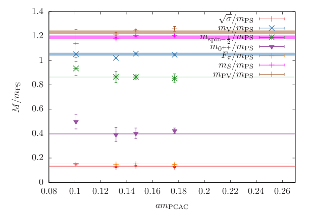


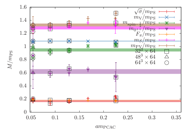
The results for the masses of the different states are shown in Figs. 1, 2, 4 and 5. First of all, it can clearly be observed that the mass hierarchy is different from the one in the chiral symmetry breaking scenario. Instead of the would-be Goldstone particle () the scalar () glueball is the lightest state in the theory. Furthermore, the ratios of different quantities divided by are not divergent in the zero fermion mass limit, as it would be the case for Goldstone particles. Instead, they approach approximately constant values. These observations are consistent with an IR conformal behaviour of the theory.
At the smallest fermion masses, in particular for at , the results deviate significantly from the expected constant mass ratios. The vector meson mass ratio is relatively stable, but for the glueball even an inversion of the mass hierarchy with is observed. The ratios of string tension and pseudoscalar decay constant over raise in this region, see Fig. 6. A similar observation has been made for the string tension in [9], where it has been traced back to a finite size effect at small . We therefore conclude that the inverted mass hierarchy at these small fermion masses is not a physical feature, but rather a finite size effect. A more detailed investigation of this effect would require simulations on very large lattices, which is beyond the scope of our current investigations. In the estimates of the mass ratios we have therefore excluded the run at , and, for the same reason, the run at , . Note that the clear distinction of the chiral symmetry breaking and the conformal scenario is quite challenging due to the limited accessible parameter space. A chiral symmetry breaking would be indicated by a divergence of the mass ratios at small fermion masses. Out data do not favour this scenario, in particular by the precise values for , but it is not excluded that it becomes dominant at even smaller fermion masses. The heavy meson mass ratios and might in addition have a subleading linear behaviour that we are not able to determine reliably.
| State | Ref. [27] | ||
|---|---|---|---|
| 1.0825(58) | 1.051(12) | 1.044(43) | |
| 1.285(24) | 1.190(14) | 1.222(52) | |
| 1.329(21) | 1.232(13) | 1.26(35) | |
| 0.620(35) | 0.398(48) | 0.458(15) | |
| 0.1831(23) | 0.15156(72) | 0.178(5) | |
| 0.171(16) | 0.1327(44) | 0.0959(14) – 0.1319(10) | |
| 0.948(24) | 0.86394(52) | – | |
| range | 0.1808(22) – 0.2490(12) | 0.2457(12) – 0.26776(42) | 0.1872(84) – 0.2323(35) |
| range | 0.29986(46) – 0.58848(98) | 0.5360(25) – 0.57247(16) | 0.6401(11) – 1.183(1) |
In spite of the limitations on the mass ranges, we are able to provide estimates for the universal ratios between the different observables and the pseudoscalar meson mass . These are based on at least two values of the mass for each . The results are shown in Table 1, where also the results of [27] are presented for comparison. The general ordering of the masses at both values is preserved, but all the ratios of masses to decrease from to . For the meson masses the changes are below , and for the spin 1/2 state they are slightly larger. The glueball mass, however, gets corrections of the order of . Consequently, the gap between the glueball and the meson masses is significantly increased at the larger value. This considerable difference cannot be explained by the slightly different range of in units of for and . In particular, the range is consistent for the two values. Therefore we conclude that towards the continuum limit the difference between the scalar glueball and the rest of the spectrum is in fact increased.
We would like to note that the data in [27] are all approximately between our results at and . Hence it seems that our results at the coarse lattice spacing have larger lattice artefacts, while the finer lattice spacing is closer to the continuum limit than in [27]. The string tension deviates from this observation, but the values provided in the literature show a considerable variance and hence seem to be subject to significant systematic uncertainties. The uncertainties in our measurements are indicated by the broad plateau estimation of the mass ratio, see Fig. 6. Further details of our measurement can be found in Section V.1.
Our arguments concerning the continuum limit in this section are based simply on the asymptotic freedom of the gauge theory, which implies a decreasing lattice spacing approaching . If we assume that the theory is already close to the conformal fixed point, the differences between the results in Table 1 are an indication for scaling corrections. These effects seem to be relevant and to produce a significant correction for the mass ratio of the scalar glueball and the pseudoscalar meson mass.
V.1 Scalar glueball and string tension
The glueball appears to be the lightest scalar particle in aQCD2. Despite a possible mixing with the scalar singlet meson operators, it seems to have a reasonable overlap with the ground state in the scalar sector as will be detailed in Section V.2. Hence it provides the signal for a possible Higgs-like bound state. In some cases we have also obtained an estimate for the glueball mass (see Table 2). It appears to be lighter than the pseudoscalar singlet meson, but the systematic uncertainties are quite large.
We determine the glueball mass using as interpolating operator the fundamental plaquette built from four links and the is given by the product of eight links with suitable shape. In order to reduce the contamination from excited states and thus determining the effective mass already at small time-slice separations we used the variational method based on APE smeared operators. In total, between and smearing levels were used in the variational method, each separated by 4 or 5 steps; the smearing parameter was fixed to .
Fig. 7 shows an example of the fitted mass value for different ranges . A clear plateau appears already at . Using this approach we can determine the mass value with a relative error starting from for some ensembles.


For a theory in the confined phase, the potential between a static quark-antiquark pair in the fundamental representation grows linearly at large separations. The coefficient of the linear rise is the string tension . In a theory with adjoint matter the chromoelectric field is not screened and is a well defined quantity. In an IR conformal theory the string tension will vanish in the limit of massless fermions.
We determine the string tension from the expectation value of the Wilson loop . To this purpose we first define the generalised potential:
| (7) |
The method consists of two steps: in the first one we determine the static quark-antiquark potential fitting for every , in the interval , to the function [32]
| (8) |
in the second step we fit the potential to the form of the Cornell potential, in the interval , and we determine the value of the string tension. We have verified that, compared to supersymmetric Yang-Mills theory, the value of , in the first fit, has to be increased from the value 2 to the value 3 and the value of , in the second fit, has to be increased from 2 to 4. As a consequence, the potential is characterised by large error bars, in particular at large as can be seen in Fig. 8, and the final string tension has a relative error times larger than the case of supersymmetric Yang-Mills theory.
V.2 Singlet meson states and a second signal for the scalar channel
In our work we investigated the singlet meson sector of adjoint QCD for the first time. The measurement of these states is more challenging than for the rest of the spectrum, because their correlation functions contain disconnected fermion contributions. For the calculation of these contributions we have used the same methods that we have already applied in our studies of supersymmetric Yang-Mills theory. It turns out that there are significant systematic uncertainties in the measurement of these states and therefore the reported errors are most likely underestimated. The results for the masses are shown in Table 2.
The primary aim of these investigation is to obtain a second signal for the scalar channel. The has the same quantum numbers as the glueball, and hence both operators have overlap with the ground state in the scalar channel. The overlap with the ground state might, however, be small such that a significant contribution from excited states is present. In the case of supersymmetric Yang-Mills theory and one-flavour adjoint QCD it turned out that there is a reasonable agreement between the two signals in the scalar channel.
| 24 | 64 | 1.5 | 0.1325 | 0.511(53) | 0.634(14) | 0.58710(27) | 0.767(12) | 0.350(25) | 0.62(9) |
| 32 | 64 | 1.5 | 0.1335 | 0.295(70) | 0.474(49) | 0.44212(28) | 0.561(12) | 0.260(25) | 0.44(5) |
| 48 | 64 | 1.5 | 0.1344 | 0.320(69) | 0.342(36) | 0.29986(46) | 0.3816(87) | 0.180(30) | 0.32(4) |
| 32 | 64 | 1.7 | 0.1285 | 0.515(52) | 0.574(28) | 0.57247(16) | 0.6902(62) | 0.230(25) | 0.43(1) |
| 32 | 64 | 1.7 | 0.1290 | 0.419(66) | 0.504(31) | 0.5360(25) | 0.6312(23) | 0.210(30) | 0.36(2) |
In aQCD2, the measurement of the connected and disconnected contributions of the correlators leads to quite different results in the scalar and the pseudoscalar case. While for the meson the disconnected contribution is almost negligible, see Fig. 9 (rhs), it is the dominant contribution for the , as shown in Fig. 9 (lhs). The large disconnected contribution is the reason for the large difference between and . The scalar singlet meson mass () is consequently much smaller than the mass in the triplet channel (). Nevertheless, there is no degeneracy with the light scalar glueball. The mass of the scalar singlet meson is of the order of the pseudoscalar meson mass or even lighter. It is interesting that in several investigations of near IR conformal theories a similar approximate degeneracy between the scalar singlet and the pseudoscalar meson has been observed [14, 33].


Our results are an indication that the ground state in the scalar channel is dominated by the glueball state. An analysis of the mixing between the glueball and the meson will provide further information about the overlap of the different operators with the lightest state.
Taking into account the systematic error in the evaluation of the singlet mesons, the meson is almost degenerate with the pseudoscalar meson. The difference between these states, which in QCD is related to the axial anomaly, is negligible within the current precision.
V.3 Spin one-half states and possible fractionally charged particles
A specific feature of theories with fermions in the adjoint representation of the gauge group is the presence of mixed fermion-gluon states, which do not occur in QCD. The most interesting one is a fermionic spin 1/2 particle represented by the operator
| (9) |
This particle is of particular importance in supersymmetric Yang-Mills theory, where this gluino-glue particle is the fermionic member of the scalar supermultiplet of bound states. Unbroken supersymmetry implies a degenerate mass for all the states of the supermultiplet, and hence it has the same mass as the lightest scalar and pseudoscalar particle in this model.
In aQCD2 the spin 1/2 state is relevant for phenomenological considerations, since it leads to fractionally charged particles, when a naive hypercharge assignment is assumed. Even though the mass of these particles is unknown, they have been considered to disfavour the phenomenological relevance of the theory. This was essentially one of the motivations to consider gauge theory as an alternative [34]. On the other hand, in [35] the existence of such particles has been considered as an alternative dark matter scenario.
Our results for the mass of the spin 1/2 state are contained in Table 1. They show that the mass of the spin 1/2 state is well separated from the lightest scalar particle. On the other hand, it is slightly lighter than the pseudoscalar meson, which means that it could be one of the first experimentally observable “new physics” states if this theory is realised in nature.
VI The mass anomalous dimension
Besides the ratios of different observables, also the mass anomalous dimension is an important universal property of an IR conformal gauge theory. Given the ratios and the value of , the main properties of the theory are determined. The mass anomalous dimension is of particular importance for phenomenological considerations, since in the Walking Technicolor scenario a large value of is required. We apply two different methods to determine of . They are based on the properties of particle spectrum and of the mode number.
VI.1 Scaling of the particle spectrum
| Observable | ||
|---|---|---|
| 1.5 | 0.2958(45) | |
| 1.5 | 0.295(26) | |
| 1.7 | 0.289(17) | |
| 1.7 | 0.263(28) |


The fact that the masses of all states should scale according to the universal formula
| (10) |
can be used to determine the mass anomalous dimension directly from the particle spectrum. The simplest way to determine the exponent is a linear fit in a double logarithmic representation. It turns out that for most of the masses the fit errors are large, and the fit results spread over a range of between 0.13 and 0.57. For a first estimate it is thus reasonable to consider only the most precise fits. Restricting the analysis to those states that lead to a fit error smaller than 10 %, reduces the fit to the pseudoscalar and vector meson mass. The results of this fit are shown in Table 3 and Fig. 10. From these data one obtains a mass anomalous dimension around , and there is a tendency towards a smaller value at the larger .
The large errors for several observables means that these fits represent only a rough estimate of the mass anomalous dimension. A precise determination of the mass anomalous dimension requires more control over the parameter range. This can be achieved by fits of the mode number, where an ultraviolet and infrared cutoff is introduced by the fit boundaries. The consistency with the scaling of the spectrum can then be confirmed subsequently. In the scaling formula also the approximate influence of the finite volume can be taken into account by expressing the states in units of the box size . This scaling with the value of obtained from the mode number is shown in Fig. 11 (see Section VI.2). As can be seen, within the current precision the data of the particle spectrum are consistent with the scaling obtained from the mode number. Note that in both cases the value of is preferred in comparison to by the smaller chi-square in the linear fit of .
VI.2 Mode number
| fit range | ||||
| 1.5 | 0.1325 | 0.21-0.40 | 0.39(3) | |
| 1.5 | 0.1335 | 0.21-0.40 | 0.38(1) | |
| 1.5 | 0.1344 | 0.15-0.38 | 0.380(10) | |
| 1.5 | 0.1350 | 0.11-0.37 | 0.375(4) | |
| average | 1.5 | 0.376(3) | ||
| 1.7 | 0.1285 | 0.38-0.57 | 0.270(15) | |
| 1.7 | 0.1290 | 0.36-0.59 | 0.260(20) | |
| 1.7 | 0.1300 | 0.28-0.50 | 0.285(15) | |
| average | 1.7 | 0.274(10) | ||
| Ref. [36] | 0.371(20) | |||
| Ref. [39] | 0.269(2)(5) | |||
| Ref. [43] | 0.20(3) | |||
| Ref. [10] | 0.31(6) | |||
| Ref. [9] | 0.22(6) | |||
| Ref. [19] | 0.50(26) |
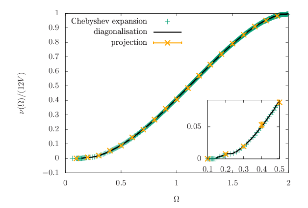

The mode number, which is the integrated eigenvalue density of the Dirac operator, allows for a more precise estimate of the mass anomalous dimension [36, 37, 38]. On the lattice the most practicable definition is obtained from the spectral density of the Dirac operator. Let
| (11) |
be the spectral density of the massless Dirac operator. The mode number , defined to be the number of eigenvalues of the positive-definite operator below some limit , is given by
| (12) |
where the cutoff for the integral is , and corresponds to the renormalised quark mass, i. e. is proportional to . Finally, the mass anomalous dimension is obtained from a fit of the mode number (see [36]) according to
| (13) |
The constant is expected to scale like , and is proportional to , but for our considerations these constants are not relevant.
The projection method used in the earlier investigations of the mode number was first proposed in [40]. It is based on a rational approximation of the projection operator in the region below a certain threshold of the eigenvalues. The mode number is hence defined as
| (14) |
where the trace is obtained by a stochastic estimate. The projection operator is approximated by means of a polynomial approximation of the step function using
| (15) |
The parameter is adjusted in such a way that the error of the approximation is minimised (see [40] for further details).
More recently a different method, based on a Chebyshev expansion of , has been proposed in [22]. We have mainly used a variant of this method, but we also checked the consistency with the projection method. For the Chebyshev expansion method the spectrum has to be rescaled to the interval according to
| (16) |
where and are the maximal and minimal eigenvalues of the operator . The integral of the spectral density of the rescaled operator multiplied by the Chebyshev polynomial of order
| (17) |
is estimated stochastically with random noise vectors :
| (18) |
Based on the orthogonality relations for the , the spectral density is now approximated by
| (19) |
The eigenvalue density of is obtained from a simple map of the the interval back to the original eigenvalue region.
The integral in the definition of the mode number can be performed analytically. In our measurements we considered polynomials of order between 2000 and 4000.


As a check we have compared the results of the two methods with the mode number obtained from a complete numerical diagonalisation of on small lattices. In addition we performed measurements with both methods on a small number of configurations on lattices. The results of these checks are shown in Figures 12 and 13. Additional investigations and comparisons will be done in the future for further understanding of the different methods. At the moment, for the present measurements of the anomalous dimension based on a limited range of both methods are compatible.
The fitting procedure of the mode number deserves special mention. Because the fitting data are strongly correlated, to determine correctly the value of , we used the usual method, taking into account the correlation matrix. As discussed in [41], to estimate correctly the value of , the square of the number of fitted data has to be smaller than the number of configurations used. Because the mode number is measured on a number of configurations ranging in the interval , the number of fitted points ranges in the interval . For comparison, the fitting parameters have been also determined by means of uncorrelated fits, using in this case a number of fitted data of the order of the number of configurations [42], giving compatible results.
Another issue in the fitting procedure is related to the fact that Eq. (13) can be used only in a certain intermediate range of eigenvalues, that can be determined only by a systematic study of the quality and the stability of the fit. As shown in Fig. 14, we fit the data for different values of the range , looking for values which guarantee a plateau in and in the value of the mass anomalous dimension .
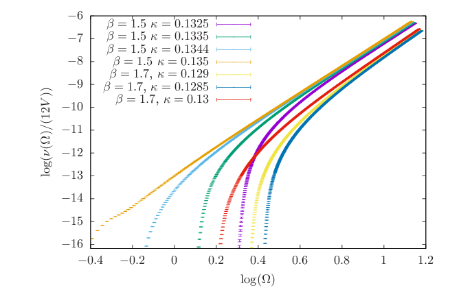
Our results for the mass anomalous dimension are presented in Fig. 15. The results of the fits are shown in Table 4. In this table we also considered the runs with sizeable finite size effects, because we assume that these effects only influence the far infrared region and not the part relevant for the fits. The results for these runs are compatible with the other runs.
The values of obtained via mode number are in reasonable agreement with those from the mass spectrum, especially for the smaller lattice spacing at .
Our result at is consistent with [36], where has been reported. The value at , however, appears to be significantly smaller. Thus there is still a remaining dependence of the mass anomalous dimension, reducing its value towards larger values. It is interesting to note that such smaller values have also been reported in other works, for example in [43].
Note that the estimates of discussed in this work show a remnant dependence on the gauge coupling, and are thus not precisely identical with the universal value at the IR fixed point. The determination of the value at the fixed-point would require to include scaling corrections in the analysis, which is beyond the present possibilities.
VII Conclusions
In this work we have presented results for gauge theory with two flavours of Dirac fermions in the adjoint representation regarding the particle spectrum and concerning general signals for conformality at two different values for the inverse gauge coupling and several masses of the two adjoint Dirac fermions. The structure of the low-lying spectrum of particle masses shows clear indications for an IR conformal behaviour. This qualitative observation was complemented with quantitative results for the universal mass ratios and the mode number.
In earlier investigations the (triplet) mesonic spectrum and the glueballs have been considered. Note in particular the detailed studies of finite volume effects in [27] and of the mode number in [36]. As shown in Table 4, these rather precise estimates for the mass anomalous dimension are not consistent with other investigations based on alternative methods. Our results indicate that the consideration of the dependence on the gauge coupling and the corresponding scaling violation provides the missing link between these estimates. At the smaller value we find, despite the differences in the lattice actions, results consistent with [27] and [36]. At the larger value, however, we find significantly lower results for the masses in units of the pseudoscalar mass, especially for the glueball, and a smaller mass anomalous dimension. Bearing in mind that different lattice actions have been used, the unimproved one in [36] and the clover improved fermion action in [43], our results indicate that the mass anomalous dimensions converge towards a universal value in the continuum limit only, if possible scaling corrections are included. It seems that towards that limit aQCD2 becomes even more conformal in the sense that the gap between the scalar particle and the rest of the spectrum is increased and the mass anomalous dimension gets smaller. In fact, our results indicate that the differences between various numerical results for the mass anomalous dimension are rather related to scaling corrections than to the differences between the considered approaches.
Our work also provides a connection to the large results presented in [39]. The mass anomalous dimension in conformal adjoint QCD is expected to depend only weakly on . Therefore the investigation in a large volume-reduced theory might be a valid approximation. The mass anomalous dimension obtained in this approach is consistent with our results at .
In addition to these results, we have also been able to investigate particle states that have not been considered before. The one with the most interesting phenomenological consequences is the spin 1/2 state. We have found that it is considerably lighter than the mesons, and therefore it might eventually be interesting from a phenomenological point of view.
The general picture of the particle spectrum in aQCD2 appears to be ordered starting with low mass pure gluonic states (glueballs), followed by heavier mixed fermion-gluon objects, and finally the rather heavy triplet mesons.
We have also measured the singlet mesons in the particle spectrum of aQCD2 for the first time. The most interesting state is the scalar singlet meson. Having the same quantum numbers as the lightest scalar particle in the theory, it may give additional information about it. Due to the dominance of the disconnected contributions, the mass of this particle is comparable or even below that of the pseudoscalar meson, the lightest meson in the triplet channel. This is similar to the observations reported in other studies [14, 33] of (near) IR conformal theories. However, the ground state in this channel seems to be dominated by the gluonic contributions, and hence the effective mass in the meson channel is still higher than the one in the glueball channel. Therefore it is not sufficient to measure only the mesonic contribution to get a complete picture for the lightest scalar in this theory.
Acknowledgments
We thank Agostino Patella, Biagio Lucini, Anna Hasenfratz, and Kieran Holland for interesting discussions.
The authors gratefully acknowledge the Gauss Centre for Supercomputing (GCS) for providing computing time for a GCS Large-Scale Project on the GCS share of the supercomputer JUQUEEN at Jülich Supercomputing Centre (JSC) and on the supercomputer SuperMUC at Leibniz Computing Centre (LRZ). GCS is the alliance of the three national supercomputing centres HLRS (Universität Stuttgart), JSC (Forschungszentrum Jülich), and LRZ (Bayerische Akademie der Wissenschaften), funded by the German Federal Ministry of Education and Research (BMBF) and the German State Ministries for Research of Baden-Württemberg (MWK), Bayern (StMWFK) and Nordrhein-Westfalen (MIWF). Further computing time has been provided by the computer cluster PALMA of the University of Münster.
References
- [1] S. Weinberg, Phys. Rev. D 13 (1976) 974.
- [2] L. Susskind, Phys. Rev. D 20 (1979) 2619.
- [3] B. Holdom, Phys. Rev. D 24 (1981) 1441.
- [4] F. Sannino and K. Tuominen, Phys. Rev. D 71 (2005) 051901 [hep-ph/0405209].
- [5] D. D. Dietrich and F. Sannino, Phys. Rev. D 75 (2007) 085018 [hep-ph/0611341].
- [6] J. Braun, C. S. Fischer and H. Gies, Phys. Rev. D 84 (2011) 034045 [arXiv:1012.4279 [hep-ph]].
- [7] S. Catterall and F. Sannino, Phys. Rev. D 76 (2007) 034504 [arXiv:0705.1664 [hep-lat]].
- [8] A. Hietanen, J. Rantaharju, K. Rummukainen and K. Tuominen, Nucl. Phys. A 820 (2009) 191C.
- [9] L. Del Debbio, B. Lucini, A. Patella, C. Pica and A. Rago, Phys. Rev. D 82 (2010) 014510 [arXiv:1004.3206 [hep-lat]].
- [10] T. DeGrand, Y. Shamir and B. Svetitsky, Phys. Rev. D 83 (2011) 074507 [arXiv:1102.2843 [hep-lat]].
- [11] T. Appelquist, G. T. Fleming, M. F. Lin, E. T. Neil and D. A. Schaich, Phys. Rev. D 84 (2011) 054501 [arXiv:1106.2148 [hep-lat]].
- [12] T. DeGrand, Y. Shamir and B. Svetitsky, Phys. Rev. D 82 (2010) 054503 [arXiv:1006.0707 [hep-lat]].
- [13] Z. Fodor, K. Holland, J. Kuti, S. Mondal, D. Nogradi and C. H. Wong, Phys. Rev. D 94 (2016) 014503 [arXiv:1601.03302 [hep-lat]].
- [14] R. C. Brower, A. Hasenfratz, C. Rebbi, E. Weinberg and O. Witzel, Phys. Rev. D 93 (2016) 075028 [arXiv:1512.02576 [hep-ph]].
- [15] A. Athenodorou, E. Bennett, G. Bergner and B. Lucini, Phys. Rev. D 91 (2015) 114508 [arXiv:1412.5994 [hep-lat]].
- [16] T. Appelquist et al., Phys. Rev. D 93 (2016) 114514 [arXiv:1601.04027 [hep-lat]].
- [17] T. DeGrand, Rev. Mod. Phys. 88 (2016) 015001 [arXiv:1510.05018 [hep-ph]].
- [18] D. Nogradi and A. Patella, Int. J. Mod. Phys. A 31 (2016) 1643003 [arXiv:1607.07638 [hep-lat]].
- [19] J. Giedt, Int. J. Mod. Phys. A 31 (2016) 1630011 [arXiv:1512.09330 [hep-lat]].
- [20] R. Foadi, M. T. Frandsen, T. A. Ryttov and F. Sannino, Phys. Rev. D 76 (2007) 055005 [arXiv:0706.1696 [hep-ph]].
- [21] G. Bergner, T. A. Ryttov and F. Sannino, JHEP 1512 (2015) 054 [arXiv:1510.01763 [hep-th]].
- [22] Z. Fodor, K. Holland, J. Kuti, S. Mondal, D. Nogradi and C. H. Wong, PoS LATTICE 2015 (2016) 310 [arXiv:1605.08091 [hep-lat]].
- [23] L. Del Debbio and R. Zwicky, Phys. Lett. B 700 (2011) 217 [arXiv:1009.2894 [hep-ph]].
- [24] A. Cheng, A. Hasenfratz, Y. Liu, G. Petropoulos and D. Schaich, Phys. Rev. D 90 (2014) 014509 [arXiv:1401.0195 [hep-lat]].
- [25] G. Münster and H. Stüwe, JHEP 1405 (2014) 034 [arXiv:1402.6616 [hep-th]].
- [26] A. Athenodorou, E. Bennett, G. Bergner, D. Elander, C.-J. D. Lin, B. Lucini and M. Piai, JHEP 1606 (2016) 114 [arXiv:1605.04258 [hep-th]].
- [27] L. Del Debbio, B. Lucini, A. Patella, C. Pica and A. Rago, Phys. Rev. D 93 (2016) 054505 [arXiv:1512.08242 [hep-lat]].
- [28] C. Morningstar and M. J. Peardon, Phys. Rev. D 69 (2004) 054501 [hep-lat/0311018].
- [29] I. Montvay and E. Scholz, Phys. Lett. B 623 (2005) 73 [hep-lat/0506006].
- [30] H. B. Meyer, H. Simma, R. Sommer, M. Della Morte, O. Witzel and U. Wolff, Comput. Phys. Commun. 176 (2007) 91 [hep-lat/0606004].
- [31] G. McGlynn and R. D. Mawhinney, Phys. Rev. D 90 (2014) 074502 [arXiv:1406.4551 [hep-lat]].
- [32] G. S. Bali, K. Schilling and C. Schlichter, Phys. Rev. D 51 (1995) 5165 [hep-lat/9409005].
- [33] Z. Fodor, K. Holland, J. Kuti, S. Mondal, D. Nogradi and C. H. Wong, PoS LATTICE 2014 (2015) 244 [arXiv:1502.00028 [hep-lat]].
- [34] A. Hietanen, C. Pica, F. Sannino and U. Søndergaard, PoS LATTICE 2013 (2014) 105 [arXiv:1311.3841 [hep-lat]].
- [35] C. Kouvaris, Phys. Rev. D 76 (2007) 015011 [hep-ph/0703266 [HEP-PH]].
- [36] A. Patella, Phys. Rev. D 86 (2012) 025006 [arXiv:1204.4432 [hep-lat]].
- [37] A. Cheng, A. Hasenfratz, G. Petropoulos and D. Schaich, PoS LATTICE 2013 (2014) 088 [arXiv:1311.1287 [hep-lat]].
- [38] Z. Fodor, K. Holland, J. Kuti, D. Nógrádi and C. H. Wong, PoS LATTICE 2013 (2014) 089 [arXiv:1402.6029 [hep-lat]].
- [39] M. García Pérez, A. González-Arroyo, L. Keegan and M. Okawa JHEP 1508 (2015) 034 [arXiv:1506.06536 [hep-lat]].
- [40] L. Giusti, C. Hoelbling, M. Lüscher and H. Wittig, Comput. Phys. Commun. 153 (2003) 31 [hep-lat/0212012].
- [41] C. Michael, Phys. Rev. D 49 (1994) 2616 [hep-lat/9310026].
- [42] C. Michael and A. McKerrell, Phys. Rev. D 51 (1995) 3745 [hep-lat/9412087].
- [43] J. Rantaharju, T. Rantalaiho, K. Rummukainen and K. Tuominen, Phys. Rev. D 93 (2016) 094509 [arXiv:1510.03335 [hep-lat]].
Appendix A Data
| 24 | 64 | 1.5 | 0.13 | 0.0477(48) | 0.22429(88) | 0.1573(12) | 0.90080(67) | 2130 |
| 24 | 64 | 1.5 | 0.1315 | 0.0229(22) | 0.16775(25) | 0.12891(44) | 0.72149(44) | 9900 |
| 24 | 64 | 1.5 | 0.1325 | 0.0081(17) | 0.128730(46) | 0.10634(27) | 0.58710(27) | 9800 |
| 24 | 64 | 1.5 | 0.135 | 0.0037(40) | 0.03136(15) | 0.0514(29) | 0.1593(20) | 1720 |
| 32 | 64 | 1.5 | 0.13 | 0.0388(30) | 0.22539(47) | 0.1561(13) | 0.90030(91) | 1480 |
| 32 | 64 | 1.5 | 0.1325 | 0.0109(15) | 0.128840(55) | 0.10617(40) | 0.58848(98) | 3448 |
| 32 | 64 | 1.5 | 0.1335 | 0.0035(15) | 0.089619(74) | 0.08125(28) | 0.44212(28) | 5627 |
| 32 | 64 | 1.5 | 0.135 | 0.00140(60) | 0.030414(45) | 0.04204(68) | 0.17063(65) | 4432 |
| 48 | 64 | 1.5 | 0.1344 | 0.0030(13) | 0.054202(59) | 0.05645(47) | 0.29986(46) | 1122 |
| 64 | 64 | 1.5 | 0.1344 | 0.00395(12) | 0.05417(11) | 0.0576(10) | 0.3009(15) | 418 |
| 32 | 64 | 1.7 | 0.1275 | 0.00708(41) | 0.17697(22) | 0.09717(29) | 0.66093(22) | 5069 |
| 32 | 64 | 1.7 | 0.1285 | 0.00605(21) | 0.147091(22) | 0.08690(16) | 0.57247(16) | 11901 |
| 32 | 64 | 1.7 | 0.129 | 0.00461(20) | 0.131717(22) | 0.08007(14) | 0.5360(25) | 11891 |
| 32 | 64 | 1.7 | 0.13 | 0.00366(34) | 0.100878(47) | 0.06591(23) | 0.42116(32) | 3941 |
| 24 | 64 | 1.5 | 0.13 | 0.9622(12) | 0.933(14) | 0.490(70) | 1.179(97) | 1.288(18) |
| 24 | 64 | 1.5 | 0.1315 | 0.77990(45) | 0.727(19) | 0.470(25) | 0.983(14) | 1.029(21) |
| 24 | 64 | 1.5 | 0.1325 | 0.63742(40) | 0.551(23) | 0.350(25) | 0.767(12) | 0.793(21) |
| 24 | 64 | 1.5 | 0.135 | 0.1802(43) | 0.292(13) | 0.190(30) | 0.400(22) | 0.38(11) |
| 32 | 64 | 1.5 | 0.13 | 0.9628(25) | 0.917(18) | 0.48(20) | 1.223(41) | 1.358(29) |
| 32 | 64 | 1.5 | 0.1325 | 0.6387(11) | 0.554(15) | 0.390(35) | 0.779(19) | 0.796(24) |
| 32 | 64 | 1.5 | 0.1335 | 0.47937(56) | 0.406(22) | 0.260(25) | 0.561(12) | 0.585(18) |
| 32 | 64 | 1.5 | 0.135 | 0.18111(91) | 0.282(25) | 0.220(35) | – | 0.299(24) |
| 48 | 64 | 1.5 | 0.1344 | 0.31963(99) | 0.296(12) | 0.180(30) | 0.3816(87) | 0.390(15) |
| 64 | 64 | 1.5 | 0.1344 | 0.3272(27) | 0.248(12) | 0.26(15) | 0.3700(72) | 0.399(37) |
| 32 | 64 | 1.7 | 0.1275 | 0.69117(32) | 0.564(24) | 0.280(15) | 0.7967(72) | 0.832(13) |
| 32 | 64 | 1.7 | 0.1285 | 0.60436(94) | 0.4945(92) | 0.230(25) | 0.6902(62) | 0.7115(56) |
| 32 | 64 | 1.7 | 0.129 | 0.54693(26) | 0.464(22) | 0.210(30) | 0.6312(23) | 0.6514(38) |
| 32 | 64 | 1.7 | 0.13 | 0.44244(62) | 0.394(24) | 0.210(25) | – | 0.479(48) |