跳到论文正文
W Papers独立论文阅读器 arXiv:1610.01297 论文正文 计算阅读时间 · 0%
引用这篇论文根据当前论文元数据生成,正式投稿前建议核对。


License: arXiv.org perpetual non-exclusive license
arXiv:1610.01297v4 [cs.RO] 07 Apr 2017

Robust Quaternion-based Cooperative Manipulation without Force/Torque Information footnoteinfo

This work was supported by the H2020 ERC Starting Grand BUCOPHSYS, the Swedish Research Council (VR), the Knut och Alice Wallenberg Foundation and the European Union’s Horizon 2020 Research and Innovation Programme under the Grant Agreement No. 644128 (AEROWORKS).
Christos K. Verginis    Matteo Mastellaro    Dimos V. Dimarogonas Address: KTH Royal Institute of Technology, Stockholm, CO 10044 Sweden (e-mail: {cverginis, matteoma, dimos}@kth.se)
Abstract

This paper proposes a task-space control protocol for the collaborative manipulation of a single object by NN robotic agents. The proposed methodology is decentralized in the sense that each agent utilizes information associated with its own and the object’s dynamic/kinematic parameters and no on-line communication takes place. Moreover, no feedback of the contact forces/torques is required, therefore employment of corresponding sensors is avoided. An adaptive version of the control scheme is also introduced, where the agents’ and object’s dynamic parameters are considered unknown. We also use unit quaternions to represent the object’s orientation. In addition, load sharing coefficients between the agents are employed and internal force regulation is guaranteed. Finally, experimental studies with two robotic arms verify the validity and effectiveness of the proposed control protocol.

keywords
Robotic manipulators, Multi-agent systems, Cooperative control, Adaptive control, Robust control.

1 Introduction

Multi-agent manipulation has gained a notable amount of attention lately. Difficult tasks including manipulation of heavy loads that cannot be handled by a single robotic arm necessitate the employment of multiple agents. Early works develop control architectures where the robotic agents communicate and share information with each other (Schneider and Cannon, 1992), and completely decentralized schemes (Liu et al., 1996; Liu and Arimoto, 1998; Zribi and Ahmad, 1992; Khatib et al., 1996; Caccavale et al., 2000) where each agent uses only local information or observers (Gudiño-Lau et al., 2004), avoiding potential communication delays.

Impedance and force/motion control is the most common methodology utilized in the related literature (Schneider and Cannon, 1992; Caccavale et al., 2008; Heck et al., 2013; Erhart and Hirche, 2013; Kume et al., 2007; Szewczyk et al., 2002; Tsiamis et al., 2015; Ficuciello et al., 2014; Ponce-Hinestroza et al., 2016; Gueaieb et al., 2007). Most of the aforementioned works employ force/torque sensors to acquire knowledge of the manipulator-object contact forces/torques which however may result to performance decline due to sensor noise or mounting difficulties. Force/Torque sensor-free methodologies can be found in (Wen and Kreutz-Delgado, 1992; Yoshikawa and Zheng, 1993; Liu et al., 1996; Kume et al., 2007; Zribi and Ahmad, 1992), which have inspired the dynamic modeling in this work.

Another important characteristic is the representation of the agent and object orientation. The most commonly used tools for orientation representation consist of rotation matrices, Euler angles and the angle/axis convention. Rotation matrices, however, are rarely used in robotic manipulation tasks due to the difficulty of extracting an error vector from them. Moreover, the mapping from Euler angles and angle/axis values to angular velocities exhibits singularities at certain points, rendering thus these representations incompetent. On the other hand, the representation using unit quaternions, which is employed in this work, constitutes a singularity-free orientation representation, without complicating the control design. Unit quaternions are employed in (Campa et al., 2006; Caccavale et al., 2000; Caccavale et al., 2008; Aghili, 2011) for manipulation tasks and in (Erhart and Hirche, 2016) for the analysis of the interaction dynamics in cooperative manipulation.

In addition, most of the works in the related literature consider known dynamic parameters regarding the object and the robotic agents. However, the accurate knowledge of such parameters, such as masses or moments of inertia, can be a challenging issue; (Liu and Arimoto, 1998) proposes an adaptive control scheme through gain tuning and (Caccavale et al., 2000) considers the robust pose regulation problem. The adaptive control of single manipulation tasks with uncertain kinematic and dynamic parameters is tackled in (Cheah et al., 2006; Wang, 2017).

In (Erhart and Hirche, 2013) and (Erhart et al., 2013) kinematic uncertainties are considered whereas (Erhart and Hirche, 2015) performs an internal force and load distribution analysis. In (Tsiamis et al., 2015) a leader-follower scheme is employed, and in (Wang and Schwager, 2015) a decentralized force consensus algorithm is developed; (Murphey and Horowitz, 2008) and (Chaimowicz et al., 2003) address the problem employing hybrid control schemes. A formation-control approach is considered in (Bai and Wen, 2010) and a fuzzy control methodology is presented in (Li et al., 2015). In (Petitti et al., 2016) the agent dynamics are not taken into account and (Wang and Schwager, 2016) considers a kinematic decentralized approach using force feedback. Finally, mobile manipulator approaches are treated in (Sugar and Kumar, 2002; Tanner et al., 2003; Ponce-Hinestroza et al., 2016).

In this paper, we propose a novel nonlinear control scheme for trajectory tracking of an object rigidly grasped by NN robotic agents. The main novelty of our approach is the combination of i) coupled object-agents dynamic formulation which does not require contact forces/torques measurements from corresponding sensors, ii) an extension to an adaptive version, where the dynamic parameters of the object and the agents are considered unknown and iii) the employment of unit quaternions for the object orientation, avoiding thus potential representation singularities. Moreover, the overall scheme is decentralized in the sense that each agent utilizes information regarding only its own state, and internal force regulation can be also guaranteed. Furthermore, in contrast to the majority of the related literature, we utilize coefficients for load sharing among the robotic arms, which may exhibit different power capabilities. To the best of the authors’ knowledge, the integration of the aforementioned attributes for cooperative manipulation has not been addressed before, and turns out to be a challenging problem, due to the high complexity of the coupled object-agents dynamics. Finally, experimental studies verify the validity and effectiveness of the proposed framework.

The rest of the paper is organized as follows: Section 2 introduces notation and preliminary background. Section 3 describes the problem formulation and the overall system’s model. The control scheme is presented in Section 4 and Section 5 verifies our approach with an experimental setup. Finally, Section 6 concludes the paper.

2 Notation and Preliminaries

2.1 Notation

The set of positive integers is denoted as ℕ\mathbb{N} and, given n∈ℕn\in\mathbb{N}, ℝn\mathbb{R}^{n} is the real nn-coordinate space, ℝ≥0n\mathbb{R}^{n}_{\geq 0} and ℝ>0n\mathbb{R}^{n}_{>0} are the sets of real nn-vectors with all elements nonnegative and positive, respectively, and SnS^{n} is the nn-D sphere; In∈ℝ≥0n×nI_{n}\in\mathbb{R}^{n\times n}_{\geq 0} and 0n×m∈ℝn×m,n,m∈ℕ0_{n\times m}\in\mathbb{R}^{n\times m},n,m\in\mathbb{N}, denote the unit matrix and the matrix with all entries zero, respectively. The vector connecting the origins of coordinate frames {A}\{A\} and {B\{B} expressed in frame {C}\{C\} coordinates in 33D space is denoted as pB/AC∈ℝ3p^{\scriptscriptstyle C}_{{\scriptscriptstyle B/A}}\in{\mathbb{R}}^{3}. Given a∈ℝ3a\in\mathbb{R}^{3}, S⁡(a)∈ℝ3×3S(a)\in\mathbb{R}^{3\times 3} is the skew-symmetric matrix defined according to S⁡(a)​b=a×bS(a)b=a\times b. The rotation matrix from {A}\{A\} to {B}\{B\} is denoted as RB/A∈S​O​(3)R_{{\scriptscriptstyle B/A}}\in SO(3), where S​O​(3)SO(3) is the 33D rotation group. The angular velocity of frame {B}\{B\} with respect to {A}\{A\}, expressed in {C}\{C\}, is denoted as ωB/AC∈ℝ3\omega^{\scriptscriptstyle C}_{\scriptscriptstyle B/A}\in\mathbb{R}^{3} and it holds that (Siciliano et al., 2010) R˙B/A=S⁡(ωB/AA)​RB/A\dot{R}_{\scriptscriptstyle B/A}=S(\omega^{\scriptscriptstyle A}_{\scriptscriptstyle B/A})R_{\scriptscriptstyle B/A}. We further denote as ϕA/B∈𝕋3\phi_{\scriptscriptstyle A/B}\in\mathbb{T}^{3} the Euler angles representing the orientation of {B}\left\{B\right\} with respect to {A}\left\{A\right\}, where 𝕋3\mathbb{T}^{3} is the 33D torus. We also define the set 𝕄=ℝ3×𝕋3\mathbb{M}=\mathbb{R}^{3}\times\mathbb{T}^{3}. For notational brevity, when a coordinate frame corresponds to an inertial frame of reference {I}\left\{I\right\}, we will omit its explicit notation (e.g., pB=pB/II,ωB=ωB/II,RB=RB/Ip_{\scriptscriptstyle B}=p^{\scriptscriptstyle I}_{\scriptscriptstyle B/I},\omega_{\scriptscriptstyle B}=\omega^{\scriptscriptstyle I}_{\scriptscriptstyle B/I},R_{\scriptscriptstyle B}=R_{\scriptscriptstyle B/I} etc.). Finally, all vector and matrix differentiations will be with respect to an inertial frame {I}\{I\}, unless otherwise stated.

2.2 Unit Quaternions

Given two frames {A}\{A\} and {B}\{B\}, we define a unit quaternion ξB/A=[ηB/A,εB/AT]T∈S3\xi_{\scriptscriptstyle B/A}=[\eta_{\scriptscriptstyle B/A},\varepsilon^{T}_{\scriptscriptstyle B/A}]^{T}\in S^{3} describing the orientation of {B}\{B\} with respect to {A}\{A\}, with ηB/A∈ℝ,εB/A∈S2\eta_{\scriptscriptstyle B/A}\in\mathbb{R},\varepsilon_{\scriptscriptstyle B/A}\in S^{2}, subject to the constraint ηB/A2+εB/AT​εB/A=1\eta^{2}_{\scriptscriptstyle B/A}+\varepsilon^{T}_{\scriptscriptstyle B/A}\varepsilon_{\scriptscriptstyle B/A}=1. The relation between ξB/A\xi_{\scriptscriptstyle B/A} and the corresponding rotation matrix RB/AR_{\scriptscriptstyle B/A} as well as the axis/angle representation can be found in (Siciliano et al., 2010). For a given quaternion ξB/A=[ηB/A,εB/AT]T∈S3\xi_{\scriptscriptstyle B/A}=[\eta_{\scriptscriptstyle B/A},\varepsilon^{T}_{\scriptscriptstyle B/A}]^{T}\in S^{3}, its conjugate, that corresponds to the orientation of {A}\{A\} with respect to {B}\{B\}, is (Siciliano et al., 2010) ξB/A∗=[ηB/A,−εB/AT]T∈S3\xi^{*}_{\scriptscriptstyle B/A}=[\eta_{\scriptscriptstyle B/A},-\varepsilon^{T}_{\scriptscriptstyle B/A}]^{T}\in S^{3}. Moreover, given two quaternions ξi=[ηi,εiT]T,i∈{1,2}{\xi_{i}}=[\eta_{i},\varepsilon_{i}^{T}]^{T},i\in\{1,2\}, the quaternion product is defined as (Siciliano et al., 2010)

ξ1⊗ξ2=[η1​η2−ε1T​ε2η1​ε2+η2​ε1+S⁡(ε1)​ε2]∈S3.\xi_{1}\otimes\xi_{2}=\left[\begin{array}[]{c}\eta_{1}\eta_{2}-\varepsilon_{1}^{T}\varepsilon_{2}\\ \eta_{1}\varepsilon_{2}+\eta_{2}\varepsilon_{1}+S(\varepsilon_{1})\varepsilon_{2}\end{array}\right]\in S^{3}. (1)

The time derivative of a quaternion ξB/A=[ηB/A,εB/AT]T∈S3\xi_{\scriptscriptstyle B/A}=[\eta_{\scriptscriptstyle B/A},\varepsilon^{T}_{\scriptscriptstyle B/A}]^{T}\in S^{3} is given by (Siciliano et al., 2010):

ξ˙B/A=12​E​(ξB/A)​ωB/AA,\dot{\xi}_{\scriptscriptstyle B/A}=\frac{1}{2}{E(\xi_{\scriptscriptstyle B/A})\omega^{\scriptscriptstyle A}_{\scriptscriptstyle B/A}}, (2a)
where E:S3→ℝ4×3E:S^{3}\to\mathbb{R}^{4\times 3} is defined as:
E⁡(ξ)=[−εTη​I3−S⁡(ε)].E(\xi)=\left[\begin{array}[]{c}-\varepsilon^{T}\\ \eta I_{3}-S(\varepsilon)\end{array}\right].
Finally, it can be shown that ET​(ξ)​E​(ξ)=I3E^{T}(\xi)E(\xi)=I_{3} and hence
ωB/AA=2​ET​(ξB/A)​ξ˙B/A.\omega^{\scriptscriptstyle A}_{\scriptscriptstyle B/A}=2E^{T}(\xi_{\scriptscriptstyle B/A})\dot{\xi}_{\scriptscriptstyle B/A}. (2b)
Refer to caption
Figure 1: Two robotic agents rigidly grasping an object.

3 Problem Formulation

Consider NN fully actuated robotic agents rigidly grasping an object (see Fig. 1). We denote as qi∈ℝniq_{i}\in\mathbb{R}^{n_{i}} the generalized joint-space variables of the iith agent and as {Ei}\left\{E_{i}\right\}, {O}\left\{O\right\} the end-effector and object’s center of mass frames, respectively; {I}\left\{I\right\} corresponds to an inertial frame of reference, as mentioned in Section 2.1. The rigidity assumption implies that the agents can exert both forces and torques along all directions to the object. We consider that each agent has access to the position and velocity of its own joint variables and that no interaction force/torque measurements or on-line information exchange between the agents is required. Moreover, it is assumed that the desired object profile as well as relevant geometric features (e.g., center of mass location) are transmitted off-line to the agents. Finally, we consider that the agents operate away from kinematic singularity poses (Siciliano et al., 2010). In the following, we present the modeling of the coupled kinematics and dynamics of the object and the agents.

3.1 Kinematics

In view of Fig. 1, we have that:

pEi​(t)\displaystyle p_{\scriptscriptstyle E_{i}}(t) =pO​(t)+pEi/O​(qi)=pO​(t)+REi​(qi)​pEi/OEi,\displaystyle=p_{\scriptscriptstyle O}(t)+p_{\scriptscriptstyle E_{i}/O}(q_{i})=p_{\scriptscriptstyle O}(t)+R_{\scriptscriptstyle E_{i}}(q_{i})p^{\scriptscriptstyle E_{i}}_{\scriptscriptstyle E_{i}/O}, (3a)
ϕEi​(t)\displaystyle\phi_{\scriptscriptstyle E_{i}}(t) =ϕO​(t)+ϕEi/O,\displaystyle=\phi_{\scriptscriptstyle O}(t)+\phi_{\scriptscriptstyle E_{i}/O}, (3b)

∀i∈𝒩\forall i\in\mathcal{N}, where pEi,ϕEi,pO,ϕOp_{\scriptscriptstyle E_{i}},\phi_{\scriptscriptstyle E_{i}},p_{\scriptscriptstyle O},\phi_{\scriptscriptstyle O} are the iith end-effector’s and object’s pose, respectively, and pEi/OEip^{\scriptscriptstyle E_{i}}_{\scriptscriptstyle E_{i}/O} and ϕEi/O\phi_{\scriptscriptstyle E_{i}/O} are the constant distance and orientation offset between {O}\{O\} and {Ei}\{E_{i}\}, which are considered known. Differentiation of (3a) along with the fact that, due to the grasping rigidity, it holds that ωEi=ωO,\omega_{\scriptscriptstyle E_{i}}=\omega_{\scriptscriptstyle O}, leads to

vi​(t)=JOi​(qi)​vO​(t),v_{i}(t)=J_{\scriptscriptstyle O_{i}}(q_{i})v_{\scriptscriptstyle O}(t), (4)

and, by differentiation, to

v˙i​(t)=J˙Oi​(qi,q˙i)​vO​(t)+JOi​(qi)​v˙O​(t),\dot{v}_{i}(t)=\dot{J}_{\scriptscriptstyle O_{i}}(q_{i},\dot{q}_{i})v_{\scriptscriptstyle O}(t)+J_{\scriptscriptstyle O_{i}}(q_{i})\dot{v}_{\scriptscriptstyle O}(t), (5)

where vO,vi:ℝ≥0→ℝ6v_{\scriptscriptstyle O},v_{i}:\mathbb{R}_{\geq 0}\to\mathbb{R}^{6} with vO​(t)=[p˙OT​(t),ωOT​(t)]Tv_{\scriptscriptstyle O}(t)=[\dot{p}^{T}_{\scriptscriptstyle O}(t),\omega^{T}_{\scriptscriptstyle O}(t)]^{T},vi​(t)v_{i}(t) =[p˙EiT​(t),ωEiT​(t)]T=[\dot{p}^{T}_{\scriptscriptstyle E_{i}}(t),\omega^{T}_{\scriptscriptstyle E_{i}}(t)]^{T} are the object’s center of mass’ and end-effectors’ velocities respectively. Also, JOi:ℝni→ℝ6×6J_{\scriptscriptstyle O_{i}}:\mathbb{R}^{n_{i}}\to\mathbb{R}^{6\times 6} is the object-to-agent Jacobian matrix, with

JOi​(qi)=[I3S⁡(pO/Ei​(qi))03×3I3],J_{\scriptscriptstyle O_{i}}(q_{i})=\left[\begin{array}[]{cc}I_{3}&S(p_{\scriptscriptstyle O/E_{i}}(q_{i}))\\ 0_{3\times 3}&I_{3}\end{array}\right], (6)

which is always full-rank due to the grasp rigidity.

Remark 1

Each agent ii can compute pEi,ϕEip_{\scriptscriptstyle E_{i}},\phi_{\scriptscriptstyle E_{i}} and viv_{i} via its forward and differential kinematics (Siciliano et al., 2010) pEi​(t)=kpi​(qi),ϕEi​(t)=kηi​(qi)p_{\scriptscriptstyle E_{i}}(t)=k_{p_{i}}(q_{i}),\phi_{\scriptscriptstyle E_{i}}(t)=k_{\eta_{i}}(q_{i}) and vi​(t)=Ji​(qi)​q˙iv_{i}(t)=J_{i}(q_{i})\dot{q}_{i}, respectively, where kpi:ℝni→ℝ3,kηi:ℝni→𝕋3k_{p_{i}}:\mathbb{R}^{n_{i}}\to\mathbb{R}^{3},k_{\eta_{i}}:\mathbb{R}^{n_{i}}\to\mathbb{T}^{3} are the forward kinematics and Ji:ℝni→ℝ6×6J_{i}:\mathbb{R}^{n_{i}}\to\mathbb{R}^{6\times 6} is the geometric Jacobian of agent i∈𝒩i\in\mathcal{N}. In addition, since pEi/OEip^{\scriptscriptstyle E_{i}}_{\scriptscriptstyle E_{i}/O} and ϕEi/O\phi_{\scriptscriptstyle E_{i}/O} are known, pO,ϕOp_{\scriptscriptstyle O},\phi_{\scriptscriptstyle O} and vOv_{\scriptscriptstyle O} can be computed by inverting (3) and (4), respectively, without employing any sensory data for the object’s configuration. Moreover, from ϕO\phi_{\scriptscriptstyle O}, we can compute the unit quaternion ξO\xi_{\scriptscriptstyle O} (Siciliano et al., 2010) to represent the object’s orientation, since the desired pose for the object’s center of mass will be given in terms of a desired position trajectory pO,d​(t)p_{\scriptscriptstyle O,\text{d}}(t) and a desired quaternion trajectory ξO,d​(t)\xi_{\scriptscriptstyle O,\text{d}}(t).

3.2 Dynamics

Next, we consider the following second order dynamics for the object, which can be derived based on the Newton-Euler formulation:

MO​(xO)​v˙O+CO​(xO,x˙O)​vO+gO​(xO)=fO,M_{\scriptscriptstyle O}(x_{\scriptscriptstyle O})\dot{v}_{\scriptscriptstyle O}+C_{\scriptscriptstyle O}(x_{\scriptscriptstyle O},\dot{x}_{\scriptscriptstyle O})v_{\scriptscriptstyle O}+g_{\scriptscriptstyle O}(x_{\scriptscriptstyle O})=f_{\scriptscriptstyle O}, (7)

where xO:ℝ≥0→𝕄x_{\scriptscriptstyle O}:\mathbb{R}_{\geq 0}\to\mathbb{M}, with xO​(t)=[pOT​(t),ϕOT​(t)]Tx_{\scriptscriptstyle O}(t)=[p^{T}_{\scriptscriptstyle O}(t),\phi^{T}_{\scriptscriptstyle O}(t)]^{T}, MO:𝕄→ℝ6×6M_{\scriptscriptstyle O}:\mathbb{M}\to\mathbb{R}^{6\times 6} is the positive definite inertia matrix, CO:𝕄×ℝ6→ℝ6×6C_{\scriptscriptstyle O}:\mathbb{M}\times\mathbb{R}^{6}\to\mathbb{R}^{6\times 6} is the Coriolis matrix, gO:𝕄→ℝ6g_{\scriptscriptstyle O}:\mathbb{M}\to\mathbb{R}^{6} is the gravity vector, and fO∈ℝ6f_{\scriptscriptstyle O}\in\mathbb{R}^{6} is the vector of generalized forces acting on the object’s center of mass.

The task space agent dynamics are given by (Siciliano et al., 2010):

Mi​(qi)​v˙i+Ci​(qi,q˙i)​vi+gi​(qi)=ui−fi,M_{i}(q_{i})\dot{v}_{i}+C_{i}(q_{i},\dot{q}_{i})v_{i}+g_{i}(q_{i})=u_{i}-f_{i}, (8)

where Mi:ℝni→ℝ6×6M_{i}:\mathbb{R}^{n_{i}}\to\mathbb{R}^{6\times 6} is the positive definite inertia matrix, Ci:ℝni×ℝni→ℝ6×6C_{i}:\mathbb{R}^{n_{i}}\times\mathbb{R}^{n_{i}}\to\mathbb{R}^{6\times 6} is the Coriolis matrix, gi:ℝni→ℝ6g_{i}:\mathbb{R}^{n_{i}}\to\mathbb{R}^{6} is the task-space gravity term, fi∈ℝ6f_{i}\in\mathbb{R}^{6} is the vector of generalized forces that agent ii exerts on the grasping point with the object and uiu_{i} is the task space wrench acting as the control input, ∀i∈𝒩\forall i\in\mathcal{N}.

The agent dynamics (8) can be written in vector form as:

M⁡(q)​v˙+C⁡(q,q˙)​v+g⁡(q)=u−f,{M}({q})\dot{{v}}+{C}({q},\dot{{q}}){v}+{g}({q})={u}-{f}, (9)

where q=[[qiT]i∈𝒩]T∈ℝn{q}=[[q^{T}_{i}]_{i\in\mathcal{N}}]^{T}\in\mathbb{R}^{n}, with n=∑i∈𝒩nin=\sum_{i\in\mathcal{N}}n_{i}, v=[[viT]i∈𝒩]∈ℝ6​N,M=diag​{[Mi]i∈𝒩}∈ℝ6​N×6​N,C=diag​{[Ci]i∈𝒩}∈ℝ6​N×6​N,f=[[fiT]i∈𝒩]T∈ℝ6​N,u=[[uiT]i∈𝒩]T∈ℝ6​N,g=[[giT]i∈𝒩]T∈ℝ6​N{v}=[[v^{T}_{i}]_{i\in\mathcal{N}}]\in\mathbb{R}^{6N},{M}=\text{diag}\{[M_{i}]_{i\in\mathcal{N}}\}\in\mathbb{R}^{6N\times 6N},{C}=\text{diag}\{[C_{i}]_{i\in\mathcal{N}}\}\in\mathbb{R}^{6N\times 6N},{f}=[[f^{T}_{i}]_{i\in\mathcal{N}}]^{T}\in\mathbb{R}^{6N},{u}=[[u^{T}_{i}]_{i\in\mathcal{N}}]^{T}\in\mathbb{R}^{6N},{g}=[[g^{T}_{i}]_{i\in\mathcal{N}}]^{T}\in\mathbb{R}^{6N}.

Remark 2

The task space wrench uiu_{i} can be translated to joint space inputs τi∈ℝni\tau_{i}\in\mathbb{R}^{n_{i}} via τi=JiT​(qi)​ui+(Ini−JiT​(qi)​J¯iT​(qi))​τi​0\tau_{i}=J^{T}_{i}(q_{i})u_{i}+(I_{n_{i}}-J^{T}_{i}(q_{i})\bar{J}^{T}_{i}(q_{i}))\tau_{i0}, where J¯i\bar{J}_{i} is a generalized inverse of JiJ_{i} (Siciliano et al., 2010); τi​0\tau_{i0} concerns redundant agents (ni>6n_{i}>6) and does not contribute to end-effector forces.

Moreover, the following property holds:

Lemma 1

(Siciliano et al., 2010) The matrices M˙O−2​CO\dot{M}_{\scriptscriptstyle O}-2C_{\scriptscriptstyle O} and M˙i−2​Ci\dot{M}_{i}-2C_{i} are skew-symmetric.

The kineto-statics duality (Siciliano et al., 2010) along with the grasp rigidity suggest that the force fOf_{\scriptscriptstyle O} acting on the object’s center of mass and the generalized forces fi,i∈𝒩f_{i},i\in\mathcal{N}, exerted by the agents at the grasping points, are related through:

fO=GT​(q)​f,f_{\scriptscriptstyle O}=G^{T}({q}){f}, (10)

where G:ℝn→ℝ6​N×6G:\mathbb{R}^{n}\to\mathbb{R}^{6N\times 6} is the full column-rank grasp matrix, with

G⁡(q)=[JO1T​(q1),…,JONT​(qN)]T.G({q})=[J^{T}_{\scriptscriptstyle O_{1}}(q_{1}),\dots,J^{T}_{\scriptscriptstyle O_{N}}(q_{N})]^{T}.

By substituting (9) into (10), we obtain:

fO=GT​(q)​(u−M⁡(q)​v˙−C⁡(q,q˙)​v−g⁡(q)),f_{\scriptscriptstyle O}=G^{T}({q})\left({u}-{M}({q})\dot{{v}}-{C}({q},\dot{{q}}){v}-{g}({q})\right), (11)

which, after substituting (4), (5), (7), and rearranging terms, yields the overall system coupled dynamics:

M~​(q,xO)​v˙O+C~​(q,q˙,xO,x˙O)​vO+g~​(q,xO)=GT​(q)​u,\tilde{M}({q},x_{\scriptscriptstyle O})\dot{v}_{\scriptscriptstyle O}+\tilde{C}({q},\dot{{q}},x_{\scriptscriptstyle O},\dot{x}_{\scriptscriptstyle O})v_{\scriptscriptstyle O}+\tilde{g}({q},x_{\scriptscriptstyle O})=G^{T}({q}){u}, (12)

where

M~=\displaystyle\tilde{M}= MO+GT​M​G\displaystyle M_{\scriptscriptstyle O}+G^{T}{M}G (13a)
C~=\displaystyle\tilde{C}= CO+GT​C​G+GT​M​G˙\displaystyle C_{\scriptscriptstyle O}+G^{T}{C}G+G^{T}{M}\dot{G} (13b)
g~=\displaystyle\tilde{g}= gO+GT​g.\displaystyle g_{\scriptscriptstyle O}+G^{T}{g}. (13c)

Moreover, the following Lemma holds.

Lemma 2

The matrix M~\tilde{M} is symmetric and positive definite and the matrix M~˙−2​C~\dot{\tilde{M}}-2\tilde{C} is skew-symmetric.

{pf}

By employing the definition of M{M} and the positive definiteness of Mi,∀i∈𝒩M_{i},\forall i\in\mathcal{N}, it is straightforward to prove the positive definiteness of M{M}. Then, in view of (13a) and by invoking the positive definiteness of MOM_{\scriptscriptstyle O} and the fact that GG is full column-rank, we deduce the positive definiteness of M~.{\tilde{M}}.

Regarding the skew symmetry of M~˙−2​C~,\dot{\tilde{M}}-2\tilde{C}, notice first that the definitions of M,C{M},{C} as well as Lemma 1 imply the skew-symmetry of M˙−2​C\dot{{M}}-2{C}. Moreover, by defining A=G˙T​M​G˙A=\dot{G}^{T}{M}\dot{G}, we have from (13a), (13b):

M~˙−2​C~=M˙O−2​CO+GT​(M˙−2​C)​G+A−AT,\dot{\tilde{M}}-2\tilde{C}=\dot{M}_{\scriptscriptstyle O}-2C_{\scriptscriptstyle O}+G^{T}(\dot{{M}}-2{C})G+A-A^{T},

from which, by employing Lemma 1, we obtain: (M~˙−2​C~)T=−(M~˙+2​C~)(\dot{\tilde{M}}-2\tilde{C})^{T}=-(\dot{\tilde{M}}+2\tilde{C}), which completes the proof. Formally, the problem treated in this paper is the following:

Problem 1

Given a desired bounded object pose specified by pO,d​(t)∈ℝ3,ξO,d​(t)=[ηO,d,εO,dT]T∈S3p_{\scriptscriptstyle O,\text{d}}(t)\in\mathbb{R}^{3},\xi_{\scriptscriptstyle O,\text{d}}(t)=[\eta_{\scriptscriptstyle O,\text{d}},\varepsilon^{T}_{\scriptscriptstyle O,\text{d}}]^{T}\in S^{3}, with bounded first and second derivatives, find u{u} in (12) that achieves limt→∞[pO​(t)ξO​(t)]=[pO,d​(t)ξO,d​(t)]\lim\limits_{t\rightarrow\infty}\left[\begin{array}[]{c}p_{\scriptscriptstyle O}(t)\\ \xi_{\scriptscriptstyle O}(t)\end{array}\right]=\left[\begin{array}[]{c}p_{\scriptscriptstyle O,\text{d}}(t)\\ \xi_{\scriptscriptstyle O,\text{d}}(t)\end{array}\right].

4 Main Results

We need first to define the errors associated with the object pose and the desired pose trajectory. We first define the position error ep:ℝ≥0→ℝ3e_{p}:\mathbb{R}_{\geq 0}\to\mathbb{R}^{3}:

ep​(t)=pO​(t)−pO,d​(t).e_{p}(t)=p_{\scriptscriptstyle O}(t)-p_{\scriptscriptstyle O,\text{d}}(t). (14)

Since unit quaternions do not form a vector space, they cannot be subtracted to form an orientation error; instead we should use the properties of the quaternion group algebra. Let eξ=[eη,eεT]T:ℝ≥0→S3e_{\xi}=[e_{\eta},e^{T}_{\varepsilon}]^{T}:\mathbb{R}_{\geq 0}\to S^{3} be the unit quaternion describing the orientation error. Then, it holds that (Siciliano et al., 2010),

eξ​(t)=ξO,d​(t)⊗ξO∗​(t)=[ηO,d​(t)εO,d​(t)]⊗[ηO​(t)−εO​(t)],e_{\xi}(t)=\xi_{\scriptscriptstyle O,\text{d}}(t)\otimes\xi_{\scriptscriptstyle O}^{*}(t)=\begin{bmatrix}\eta_{\scriptscriptstyle O,\text{d}}(t)\\ \varepsilon_{\scriptscriptstyle O,\text{d}}(t)\end{bmatrix}\otimes\begin{bmatrix}\eta_{\scriptscriptstyle O}(t)\\ -\varepsilon_{\scriptscriptstyle O}(t)\end{bmatrix},

which, by using (1), becomes:

eξ​(t)\displaystyle e_{\xi}(t) =[eη​(t)eε​(t)]=\displaystyle=\begin{bmatrix}e_{\eta}(t)\\ e_{\varepsilon}(t)\end{bmatrix}=
=[ηO​(t)​ηO,d​(t)+εOT​(t)​εO,d​(t)ηO​(t)​εO,d​(t)−ηO,d​(t)​εO​(t)+S⁡(εO)​(t)​εO,d​(t)].\displaystyle=\begin{bmatrix}\eta_{\scriptscriptstyle O}(t)\eta_{\scriptscriptstyle O,\text{d}}(t)+\varepsilon^{T}_{\scriptscriptstyle O}(t)\varepsilon_{\scriptscriptstyle O,\text{d}}(t)\\ \eta_{\scriptscriptstyle O}(t)\varepsilon_{\scriptscriptstyle O,\text{d}}(t)-\eta_{\scriptscriptstyle O,\text{d}}(t)\varepsilon_{\scriptscriptstyle O}(t)+S(\varepsilon_{\scriptscriptstyle O})(t)\varepsilon_{\scriptscriptstyle O,\text{d}}(t)\end{bmatrix}. (15)

By taking the time derivative of (14) and (15), employing (2) and certain properties of skew-symmetric matrices (Campa et al., 2006), it can be shown that (Siciliano et al., 2010)

e˙p​(t)\displaystyle\dot{e}_{p}(t) =p˙O​(t)−p˙O,d​(t)\displaystyle=\dot{p}_{\scriptscriptstyle O}(t)-\dot{p}_{\scriptscriptstyle O,\text{d}}(t) (16a)
e˙η​(t)\displaystyle\dot{e}_{\eta}(t) =12​eεT​(t)​eω​(t)\displaystyle=\tfrac{1}{2}e^{T}_{\varepsilon}(t)e_{\omega}(t) (16b)
e˙ε​(t)\displaystyle\dot{e}_{\varepsilon}(t) =−12​(eη​(t)​I3+S⁡(eε​(t)))​eω​(t)−S⁡(eε​(t))​ωO,d​(t),\displaystyle=-\tfrac{1}{2}\left(e_{\eta}(t)I_{3}+S(e_{\varepsilon}(t))\right)e_{\omega}(t)-S(e_{\varepsilon}(t))\omega_{\scriptscriptstyle O,\text{d}}(t), (16c)

where eω:ℝ≥0→ℝ3e_{\omega}:\mathbb{R}_{\geq 0}\to\mathbb{R}^{3}, with eω​(t)=ωO​(t)−ωO,d​(t)e_{\omega}(t)=\omega_{\scriptscriptstyle O}(t)-\omega_{\scriptscriptstyle O,\text{d}}(t) and ωO,d​(t)=2​ET​(ξO,d)​ξ˙O,d​(t)\omega_{\scriptscriptstyle O,\text{d}}(t)=2E^{T}(\xi_{\scriptscriptstyle O,\text{d}})\dot{\xi}_{\scriptscriptstyle O,\text{d}}(t), as indicated by (2b).

Notice that, considering the properties of unit quaternions, when ξO=ξO,d\xi_{\scriptscriptstyle O}=\xi_{\scriptscriptstyle O,\text{d}}, then eξ​(t)=[1,01×3]T∈S3e_{\xi}(t)=[1,0_{1\times 3}]^{T}\in S^{3}. If ξO=−ξO,d\xi_{\scriptscriptstyle O}=-\xi_{\scriptscriptstyle O,\text{d}}, then eξ​(t)=[−1,01×3]T∈S3e_{\xi}(t)=[-1,0_{1\times 3}]^{T}\in S^{3}, which, however, represents the same orientation. Therefore, the control objective established in Problem 1 is equivalent to

limt→∞[ep​(t)|eη​(t)|eε​(t)]=[03×1103×1].\lim\limits_{t\to\infty}\begin{bmatrix}e_{p}(t)\\ \lvert e_{\eta}(t)\rvert\\ e_{\varepsilon}(t)\end{bmatrix}=\begin{bmatrix}0_{3\times 1}\\ 1\\ 0_{3\times 1}\end{bmatrix}. (17)

Next, we design control protocols such that the specification (17) is met. Firstly, we consider that the dynamics parameters of the object and the agents are known. Then, we extend the proposed scheme to also compensate for unknown dynamic parameters, using adaptive control techniques (Slotine and Li, 1987; Siciliano et al., 2010).

4.1 Non-Adaptive Control Scheme

Define the velocity reference signals vOr:ℝ≥0→ℝ6v^{\scriptscriptstyle r}_{\scriptscriptstyle O}:\mathbb{R}_{\geq 0}\to\mathbb{R}^{6}:

vOr​(t)\displaystyle v_{\scriptscriptstyle O}^{\scriptscriptstyle r}(t) =[p˙Or​(t)ωOr​(t)]\displaystyle=\begin{bmatrix}\dot{p}_{\scriptscriptstyle O}^{\scriptscriptstyle r}(t)\\ \omega_{\scriptscriptstyle O}^{\scriptscriptstyle r}(t)\end{bmatrix}
=[p˙O,d​(t)−kp​ep​(t)ωO,d​(t)−kε​eη​(t)​eε​(t)]=vO,d​(t)−K​e​(t),\displaystyle=\begin{bmatrix}\dot{p}_{\scriptscriptstyle O,\text{d}}(t)-k_{p}e_{p}(t)\\ \omega_{\scriptscriptstyle O,\text{d}}(t)-k_{\varepsilon}e_{\eta}(t)e_{\varepsilon}(t)\end{bmatrix}=v_{\scriptscriptstyle O,\text{d}}(t)-Ke(t), (18)

where vO,d​(t)=[p˙O,dT​(t),ωO,dT​(t)]T∈ℝ6v_{\scriptscriptstyle O,\text{d}}(t)=[\dot{p}^{T}_{\scriptscriptstyle O,\text{d}}(t),\omega^{T}_{\scriptscriptstyle O,\text{d}}(t)]^{T}\in\mathbb{R}^{6}, kp,kε∈ℝ>0k_{p},k_{\varepsilon}\in\mathbb{R}_{>0}, K=diag​{kp​I3,kε​I3}∈ℝ≥06×6K=\text{diag}\{k_{p}I_{3},k_{\varepsilon}I_{3}\}\in\mathbb{R}_{\geq 0}^{6\times 6} and e⁡(t)=[epT​(t),−eη​(t)​eεT​(t)]T∈ℝ6e(t)=[e_{p}^{T}(t),-e_{\eta}(t)e^{T}_{\varepsilon}(t)]^{T}\in\mathbb{R}^{6}.

Furthermore, define the reference velocity error ev:ℝ≥0→ℝ6e_{v}:\mathbb{R}_{\geq 0}\to\mathbb{R}^{6} as:

ev​(t)=vO​(t)−vOr​(t),e_{v}(t)=v_{\scriptscriptstyle O}(t)-v_{\scriptscriptstyle O}^{\scriptscriptstyle r}(t), (19)

and design the decentralized control law for ui:ℝ≥0→ℝ6u_{i}:\mathbb{R}_{\geq 0}\to\mathbb{R}^{6} in (12), i∈𝒩i\in\mathcal{N}, as:

ui​(t)=μi​(t)+fi,d​(t)u_{i}(t)=\mu_{i}(t)+f_{i,\text{d}}(t) (20)

where

μi​(t)=\displaystyle\mu_{i}(t)= gi+(Ci​JOi+Mi​J˙Oi)​vOr​(t)+Mi​JOi​v˙Or​(t)\displaystyle g_{i}+\left(C_{i}J_{\scriptscriptstyle O_{i}}+M_{i}\dot{J}_{\scriptscriptstyle O_{i}}\right)v_{\scriptscriptstyle O}^{\scriptscriptstyle r}(t)+M_{i}J_{\scriptscriptstyle O_{i}}\dot{v}_{\scriptscriptstyle O}^{\scriptscriptstyle r}(t)
−JOi−T​(kvi​ev​(t)+ci​e​(t))\displaystyle-J^{-T}_{\scriptscriptstyle O_{i}}\left(k_{v_{i}}e_{v}(t)+c_{i}e(t)\right)
fi,d​(t)=\displaystyle f_{i,\text{d}}(t)= ci​JOi−T​(MO​v˙Or​(t)+CO​vOr​(t)+gO),\displaystyle c_{i}J_{\scriptscriptstyle O_{i}}^{-T}\left(M_{\scriptscriptstyle O}\dot{v}_{\scriptscriptstyle O}^{\scriptscriptstyle r}(t)+C_{\scriptscriptstyle O}v_{\scriptscriptstyle O}^{\scriptscriptstyle r}(t)+g_{\scriptscriptstyle O}\right),

kvi∈ℝ>0k_{v_{i}}\in\mathbb{R}_{>0} is a positive gain, ci∈ℝ≥0c_{i}\in\mathbb{R}_{\geq 0} are load sharing coefficients with 0≤ci≤1,∀i∈𝒩,∑i∈𝒩ci=10\leq c_{i}\leq 1,\forall i\in\mathcal{N},\sum_{i\in\mathcal{N}}c_{i}=1, and we have also exploited the dependence of qi,q˙i,xO,x˙Oq_{i},\dot{q}_{i},x_{\scriptscriptstyle O},\dot{x}_{\scriptscriptstyle O} on time.

The control law (20) can be also written in vector form:

u=μ+fd,{u}={\mu}+{f}_{\text{d}}, (21)

where

μ=\displaystyle{\mu}= g+(C​G+M​G˙)​vOr​(t)+M​G​v˙Or​(t)\displaystyle{g}+\left({C}G+{M}\dot{G}\right)v_{\scriptscriptstyle O}^{\scriptscriptstyle r}(t)+{M}G\dot{v}_{\scriptscriptstyle O}^{\scriptscriptstyle r}(t)
−G~T​(Kv​ev​(t)+Cf​e​(t))\displaystyle-\tilde{G}^{T}\left({K}_{v}e_{v}(t)+C_{f}e(t)\right)
fd=\displaystyle{f}_{\text{d}}= G~T​Cf​(MO​v˙Or​(t)+CO​vOr​(t)+gO),\displaystyle\tilde{G}^{T}C_{f}\left(M_{\scriptscriptstyle O}\dot{v}_{\scriptscriptstyle O}^{\scriptscriptstyle r}(t)+C_{\scriptscriptstyle O}v_{\scriptscriptstyle O}^{\scriptscriptstyle r}(t)+g_{\scriptscriptstyle O}\right),

Kv=[kv1​I6,…,kvN​I6]T∈ℝ6​N×6{K}_{v}=[k_{v_{1}}I_{6},\dots,k_{v_{N}}I_{6}]^{T}\in\mathbb{R}^{6N\times 6}, Cf=[c1​I6,…,cN​I6]TC_{f}=[c_{1}I_{6},\dots,c_{N}I_{6}]^{T} ∈ℝ6​N×6\in\mathbb{R}^{6N\times 6}, fd=[[fi,dT]i∈𝒩]T∈ℝ6​Nf_{\text{d}}=[[f^{T}_{i,\text{d}}]_{i\in\mathcal{N}}]^{T}\in\mathbb{R}^{6N}, and finally, G~=diag​{[JOi−1]i∈𝒩}∈ℝ6​N×6​N\tilde{G}=\text{diag}\{[J^{-1}_{\scriptscriptstyle O_{i}}]_{i\in\mathcal{N}}\}\in\mathbb{R}^{6N\times 6N}.

By employing the fact that GT​G~T=[I6,…,I6]∈ℝ6×6​NG^{T}\tilde{G}^{T}=[I_{6},\dots,I_{6}]\in\mathbb{R}^{6\times 6N} as well as ∑i∈𝒩ci=1\sum_{i\in\mathcal{N}}c_{i}=1, we multiply (21) by GTG^{T} to obtain:

GT​u=M~​v˙Or​(t)+C~​vOr​(t)+g~−∑i∈𝒩kvi​ev​(t)−e⁡(t),G^{T}{u}=\tilde{M}\dot{v}^{\scriptscriptstyle r}_{\scriptscriptstyle O}(t)+\tilde{C}v^{\scriptscriptstyle r}_{\scriptscriptstyle O}(t)+\tilde{g}-\sum_{i\in\mathcal{N}}k_{v_{i}}e_{v}(t)-e(t), (22)

that will be used in the sequel.

The following theorem summarizes the main results of this subsection.

Theorem 1.

Consider NN robotic agents rigidly grasping an object with coupled dynamics described by (12) under the control protocol (21). Then, under the assumption eη​(0)≠0e_{\eta}(0)\neq 0, the object pose converges asymptotically to the desired one with all closed loop signals being bounded, i.e., Problem 1 is solved.

{pf}

Consider the positive definite and radially unbounded Lyapunov function :

V⁡(ep,eη,ev,t)=\displaystyle V(e_{p},e_{\eta},e_{v},t)= 12​epT​ep+eη2−1+eεT​eε\displaystyle\frac{1}{2}{e_{p}^{T}}{e_{p}}+e_{\eta}^{2}-1+{e_{\varepsilon}^{T}}{e_{\varepsilon}}
+12​evT​M~​(q⁡(t),xO​(t))​ev.\displaystyle+\frac{1}{2}e_{v}^{T}\tilde{M}(q(t),x_{\scriptscriptstyle O}(t))e_{v}.

By differentiating VV with respect to time and substituting the error dynamics (16), we obtain:

V˙=\displaystyle\dot{V}= epT​e˙p+eη​eεT​eω+evT​M~​e˙v+12​evT​M~˙​ev\displaystyle e_{p}^{T}\dot{e}_{p}+e_{\eta}e_{\varepsilon}^{T}e_{\omega}+e_{v}^{T}\tilde{M}\dot{e}_{v}+\tfrac{1}{2}e_{v}^{T}\dot{\tilde{M}}e_{v}
=\displaystyle= epT​(p˙O−p˙O,d)+eη​eεT​(ωO−ωO,d)+\displaystyle e_{p}^{T}(\dot{p}_{\scriptscriptstyle O}-\dot{p}_{\scriptscriptstyle O,\text{d}})+e_{\eta}e_{\varepsilon}^{T}(\omega_{\scriptscriptstyle O}-\omega_{\scriptscriptstyle O,\text{d}})+
evT​M~​(v˙O−v˙Or)+12​evT​M~˙​ev,\displaystyle e_{v}^{T}\tilde{M}(\dot{v}_{\scriptscriptstyle O}-\dot{v}_{\scriptscriptstyle O}^{\scriptscriptstyle r})+\frac{1}{2}e_{v}^{T}\dot{\tilde{M}}e_{v},

from which, in view of (18), (19) and (12), we derive:

V˙=\displaystyle\dot{V}= −eT​K​e+eT​ev+evT​(GT​u−C~​vO−g~)−\displaystyle-{e^{T}Ke}+{e^{T}e_{v}}+{e_{v}^{T}}\left(G^{T}{u}-{\tilde{C}v_{{\scriptscriptstyle O}}-\tilde{g}}\right)-
evT​M~​v˙Or+12​evT​M~˙​ev\displaystyle{e_{v}^{T}}{\tilde{M}}{\dot{v}_{{\scriptscriptstyle O}}^{{\scriptscriptstyle r}}}+\frac{1}{2}{e_{v}^{T}}{\dot{\tilde{M}}}{e_{v}}
=\displaystyle= −eT​K​e+eT​ev+evT​(GT​u−C~​vOr−g~)−\displaystyle-{e^{T}Ke}+{e^{T}e_{v}}+{e_{v}^{T}}\left(G^{T}{u}-{\tilde{C}v_{{\scriptscriptstyle O}}^{{\scriptscriptstyle r}}-\tilde{g}}\right)-
evT​M~​v˙Or+evT​(12​M~˙−C~)​ev.\displaystyle{e_{v}^{T}}{\tilde{M}}{\dot{v}_{{\scriptscriptstyle O}}^{{\scriptscriptstyle r}}}+{e_{v}^{T}}\left(\frac{1}{2}{\dot{\tilde{M}}}-{\tilde{C}}\right){e_{v}}.

Then, by employing Lemma 2, V˙\dot{V} becomes:

V˙=−eT​K​e−evT​(−e+M~​v˙Or+C~​vor+g~−GT​u),\dot{V}=-{e^{T}Ke}-{e_{v}^{T}}(-{e}+{\tilde{M}}{\dot{v}_{{\scriptscriptstyle O}}^{{\scriptscriptstyle r}}}+{\tilde{C}v_{{\scriptscriptstyle o}}^{{\scriptscriptstyle r}}+\tilde{g}-}G^{T}{u}),

and after substituting (22):

V˙=−kp​epT​ep−kε​eη2​eεT​eε−∑i∈𝒩kvi​evT​ev,\dot{V}=-k_{p}e_{p}^{T}e_{p}-k_{\varepsilon}e^{2}_{\eta}e_{\varepsilon}^{T}e_{\varepsilon}-\sum_{i\in\mathcal{N}}k_{v_{i}}e_{v}^{T}e_{v}, (23)

which is non-positive. We conclude therefore that the system is stable and VV is a non-increasing function, deducing the boundedness of ep,eη,eε,ev.e_{p},e_{\eta},e_{\varepsilon},e_{v}. Hence, invoking also the boundedness of pO,dp_{\scriptscriptstyle O,\text{d}} and ωO,d\omega_{\scriptscriptstyle O,\text{d}} and of their derivatives, we employ (18) to prove the boundedness of vOrv_{\scriptscriptstyle O}^{\scriptscriptstyle r} and (19) to prove the boundedness of vOv_{\scriptscriptstyle O} and therefore of vi,v_{\scriptscriptstyle i}, since the boundedness of JOiJ_{\scriptscriptstyle O_{i}} and GG is straightforward. From the aforementioned conclusions, invoking also the fact that Mi​(⋅),Ci​(⋅),MO​(⋅),gi​(⋅),CO​(⋅),gO​(⋅)M_{i}(\cdot),C_{i}(\cdot),M_{\scriptscriptstyle O}(\cdot),g_{i}(\cdot),C_{\scriptscriptstyle O}(\cdot),g_{\scriptscriptstyle O}(\cdot) are continuous functions, we can deduce the boundedness of qiq_{i} and q˙i,∀i∈𝒩\dot{q}_{i},\forall i\in\mathcal{N} and of M~,C~,g~\tilde{M},\tilde{C},\tilde{g}. Moreover, the error derivatives (16a)-(16c) are all bounded and thus, in view of (18), v˙Or\dot{v}_{\scriptscriptstyle O}^{\scriptscriptstyle r} is bounded as well. Hence, we also deduce the boundedness of uiu_{i}. Finally, by differentiating (19) and substituting (12) and (21) we also deduce the boundedness of e˙v\dot{e}_{v} and therefore of v˙O.\dot{v}_{\scriptscriptstyle O}.

Combining the aforementioned statements we can conclude the boundedness of V¨\ddot{V} and hence the uniform continuity of V˙\dot{V}. Invoking Barbalat’s lemma (Slotine et al., 1991), we deduce that V˙→0\dot{V}\rightarrow 0 and therefore through (23) that (ep,eη​eε,ev)→(03×1,03×1,06×1)(e_{p},e_{\eta}e_{\varepsilon},e_{v})\rightarrow(0_{\scriptscriptstyle 3\times 1},0_{\scriptscriptstyle 3\times 1},0_{\scriptscriptstyle 6\times 1}). The equilibrium eη=0e_{\eta}=0 can be proven to be unstable (Mayhew et al., 2011) and hence, since eη​(0)≠0e_{\eta}(0)\neq 0, we conclude that (ep,eε,ev)→(03×1,03×1,06×1)(e_{p},e_{\varepsilon},e_{v})\rightarrow(0_{\scriptscriptstyle 3\times 1},0_{\scriptscriptstyle 3\times 1},0_{\scriptscriptstyle 6\times 1}). Furthermore, we also conclude that eη2→1e_{\eta}^{2}\rightarrow 1 since eξ∈S3e_{\xi}\in S^{3} is a unit quaternion, which leads to the completion of the proof.

Remark 4.1.

The assumption eη​(0)≠0e_{\eta}(0)\neq 0 is a necessary assumption to guarantee asymptotic stability of the orientation error eξe_{\xi}. In terms of Euler angles, it states that the initial orientation errors (in the x,y,zx,y,z directions) should not be 180180 degrees.

4.2 Adaptive Control Scheme

Consider now that the dynamic parameters of the object and the agents (e.g., masses and inertia moments), are unknown. We propose an adaptive version of (21) that does not incorporate the aforementioned parameters and still guarantees the solution of Problem 1.

It can be shown (Siciliano et al., 2010) that the object and agent dynamics can be written in the form:

Mi​(qi)​v˙i+Ci​(qi,q˙i)​vi+gi​(qi)=Hi​(qi,q˙i,vi,v˙i)​θi\displaystyle M_{i}(q_{i})\dot{v}_{i}+C_{i}(q_{i},\dot{q}_{i})v_{i}+g_{i}(q_{i})=H_{i}(q_{i},\dot{q}_{i},v_{i},\dot{v}_{i})\theta_{i} (24a)
MO​(xO)​v˙O+CO​(xO,x˙O)​vO+gO​(xO)=\displaystyle M_{\scriptscriptstyle O}(x_{\scriptscriptstyle O})\dot{v}_{\scriptscriptstyle O}+C_{\scriptscriptstyle O}(x_{\scriptscriptstyle O},\dot{x}_{\scriptscriptstyle O})v_{\scriptscriptstyle O}+g_{\scriptscriptstyle O}(x_{\scriptscriptstyle O})=
YO​(xO,x˙O,vO,v˙O)​θO,\displaystyle\hskip 125.19194ptY_{\scriptscriptstyle O}(x_{\scriptscriptstyle O},\dot{x}_{\scriptscriptstyle O},v_{\scriptscriptstyle O},\dot{v}_{\scriptscriptstyle O})\theta_{\scriptscriptstyle O}, (24b)

∀i∈𝒩\forall i\in\mathcal{N}, where θi∈ℝℓ,θO∈ℝℓO\theta_{i}\in\mathbb{R}^{\ell},\theta_{\scriptscriptstyle O}\in\mathbb{R}^{\ell_{\scriptscriptstyle O}} are vectors of unknown but constant dynamic parameters of the agents and the object, appearing in the terms Mi,Ci,giM_{i},C_{i},g_{i} and MO,CO,gOM_{\scriptscriptstyle O},C_{\scriptscriptstyle O},g_{\scriptscriptstyle O}, respectively, and Hi∈ℝ6×ℓ,i∈𝒩,YO∈ℝ6×ℓOH_{i}\in\mathbb{R}^{6\times\ell},i\in\mathcal{N},Y_{\scriptscriptstyle O}\in\mathbb{R}^{6\times\ell_{\scriptscriptstyle O}} are known regressor matrices, independent of θi,θO\theta_{i},\theta_{\scriptscriptstyle O}. It is worth noting that the choice for ℓ\ell and ℓO\ell_{\scriptscriptstyle O} is not unique and depends on the factorization method used (Siciliano et al., 2010). In the same vein, since JOiJ_{\scriptscriptstyle O_{i}}, as given in (6), depends only on qiq_{i} and not on θi,θO,∀i∈𝒩\theta_{i},\theta_{\scriptscriptstyle O},\forall i\in\mathcal{N}, we can write:

JOiT​Mi​JOi​v˙i+(JOiT​Mi​J˙Oi+JOiT​Ci​JOi)​vi+JOiT​gi=\displaystyle J^{T}_{\scriptscriptstyle O_{i}}M_{i}J_{\scriptscriptstyle O_{i}}\dot{v}_{i}+(J^{T}_{\scriptscriptstyle O_{i}}M_{i}\dot{J}_{\scriptscriptstyle O_{i}}+J^{T}_{\scriptscriptstyle O_{i}}C_{i}J_{\scriptscriptstyle O_{i}})v_{i}+J^{T}_{\scriptscriptstyle O_{i}}g_{i}=
Yi​(qi,q˙i,vi,v˙i)​θi,\displaystyle Y_{i}(q_{i},\dot{q}_{i},v_{i},\dot{v}_{i})\theta_{i}, (25)

where Yi∈ℝ6×ℓY_{i}\in\mathbb{R}^{6\times\ell} is another regressor matrix independent of θi,θO\theta_{i},\theta_{\scriptscriptstyle O}. Hence, in view of (13), (24) and (25), the left-hand side of (12) can be written as:

M~​(q,xO)​v˙O+\displaystyle\hskip-6.25958pt\tilde{M}({q},x_{\scriptscriptstyle O})\dot{v}_{\scriptscriptstyle O}+ C~​(q,q˙,xO,x˙O)​vO+g~​(q,xO)=\displaystyle\tilde{C}({q},\dot{{q}},x_{\scriptscriptstyle O},\dot{x}_{\scriptscriptstyle O})v_{\scriptscriptstyle O}+\tilde{g}({q},x_{\scriptscriptstyle O})=
YO​(xO,x˙O,vO,v˙O)​θO+YT​(q,q˙,vO,v˙O)​θ\displaystyle Y_{\scriptscriptstyle O}(x_{\scriptscriptstyle O},\dot{x}_{\scriptscriptstyle O},v_{\scriptscriptstyle O},\dot{v}_{\scriptscriptstyle O})\theta_{\scriptscriptstyle O}+Y^{T}({q},\dot{{q}},v_{\scriptscriptstyle O},\dot{v}_{\scriptscriptstyle O})\theta (26)

where Y⁡(q,q˙,vO,v˙O)=[Y1​(q1,q˙1,vO,v˙O),…,YN​(qN,q˙N,vO,v˙O)]T∈ℝN​ℓ×6Y({q},\dot{{q}},v_{\scriptscriptstyle O},\dot{v}_{\scriptscriptstyle O})=[Y_{1}(q_{1},\dot{q}_{1},v_{\scriptscriptstyle O},\dot{v}_{\scriptscriptstyle O}),\dots,Y_{N}(q_{N},\dot{q}_{N},\\ v_{\scriptscriptstyle O},\dot{v}_{\scriptscriptstyle O})]^{T}\in\mathbb{R}^{N\ell\times 6} and θ=[[θiT]i∈𝒩]T∈ℝN​ℓ\theta=[[\theta^{T}_{i}]_{i\in\mathcal{N}}]^{T}\in\mathbb{R}^{N\ell}.

Let us now denote as θ^Oi:ℝ≥0→ℝℓO\hat{\theta}^{i}_{\scriptscriptstyle O}:\mathbb{R}_{\geq 0}\to\mathbb{R}^{\ell_{\scriptscriptstyle O}} and θ^i:ℝ≥0→ℝℓ\hat{\theta}_{i}:\mathbb{R}_{\geq 0}\to\mathbb{R}^{\ell} the estimates of θO\theta_{\scriptscriptstyle O} and θi\theta_{i}, respectively, by agent i∈𝒩i\in\mathcal{N}, and the corresponding stack vectors θ^O​(t)=[[(θ^Oi​(t))T]i∈𝒩]T∈ℝN​ℓO,θ^​(t)=[[θ^iT​(t)]i∈𝒩]T∈ℝN​ℓ\hat{\theta}_{\scriptscriptstyle O}(t)=[[(\hat{\theta}^{i}_{\scriptscriptstyle O}(t))^{T}]_{i\in\mathcal{N}}]^{T}\in\mathbb{R}^{N\ell_{\scriptscriptstyle O}},\hat{\theta}(t)=[[\hat{\theta}^{T}_{i}(t)]_{i\in\mathcal{N}}]^{T}\in\mathbb{R}^{N\ell}, for which we formulate the associated errors eθO:ℝ≥0→ℝN​ℓO,eθ:ℝ≥0→ℝN​ℓe_{\theta_{\scriptscriptstyle O}}:\mathbb{R}_{\geq 0}\to\mathbb{R}^{N\ell_{\scriptscriptstyle O}},e_{\theta}:\mathbb{R}_{\geq 0}\to\mathbb{R}^{N\ell} as

eθO​(t)=\displaystyle e_{\theta_{\scriptscriptstyle O}}(t)= [eθO1​(t)eθON​(t)]=[θO−θ^O1​(t)θO−θ^ON​(t)]=θ¯O−θ^O​(t)\displaystyle\begin{bmatrix}e^{1}_{\theta_{\scriptscriptstyle O}}(t)\\ \vdots\\ e^{N}_{\theta_{\scriptscriptstyle O}}(t)\end{bmatrix}=\begin{bmatrix}\theta_{\scriptscriptstyle O}-\hat{\theta}^{1}_{\scriptscriptstyle O}(t)\\ \vdots\\ \theta_{\scriptscriptstyle O}-\hat{\theta}^{N}_{\scriptscriptstyle O}(t)\end{bmatrix}=\bar{\theta}_{\scriptscriptstyle O}-\hat{\theta}_{\scriptscriptstyle O}(t) (27a)
eθ​(t)=\displaystyle e_{\theta}(t)= [eθ1​(t)eθN​(t)]=[θ1−θ^1​(t)θN−θ^N​(t)]=θ−θ^​(t),\displaystyle\begin{bmatrix}e_{\theta_{1}}(t)\\ \vdots\\ e_{\theta_{N}}(t)\end{bmatrix}=\begin{bmatrix}\theta_{1}-\hat{\theta}_{1}(t)\\ \vdots\\ \theta_{N}-\hat{\theta}_{N}(t)\end{bmatrix}=\theta-\hat{\theta}(t), (27b)

∀i∈𝒩\forall i\in\mathcal{N}, where θ¯O=[θOT,…,θOT⏟N​times]T∈ℝN​ℓO\bar{\theta}_{\scriptscriptstyle O}=[\underbrace{\theta^{T}_{\scriptscriptstyle O},\dots,\theta^{T}_{\scriptscriptstyle O}}_{N\text{times}}]^{T}\in\mathbb{R}^{N\ell_{\scriptscriptstyle O}}.

Then, with the reference velocity signal vOrv^{\scriptscriptstyle r}_{\scriptscriptstyle O} defined as in (18) and the corresponding error eve_{v} as in (19), we design the adaptive control law ui:ℝ≥0→ℝ6u_{i}:\mathbb{R}_{\geq 0}\to\mathbb{R}^{6} in (12), for each agent i∈𝒩i\in\mathcal{N}, as:

ui​(t)=\displaystyle u_{i}(t)= JOi−T​(Yi​(qi,q˙i,vOr,v˙Or)​θ^i​(t)−ci​e​(t)−kvi​ev​(t)CLOSE\displaystyle J^{-T}_{\scriptscriptstyle O_{i}}\left(Y_{i}(q_{i},\dot{q}_{i},v^{\scriptscriptstyle r}_{\scriptscriptstyle O},\dot{v}^{\scriptscriptstyle r}_{\scriptscriptstyle O})\hat{\theta}_{i}(t)-c_{i}e(t)-k_{v_{i}}e_{v}(t)\right.
OPEN+ci​YO​(xO,x˙O,vOr,v˙Or)​θ^Oi​(t)),\displaystyle\left.+c_{i}Y_{\scriptscriptstyle O}(x_{\scriptscriptstyle O},\dot{x}_{\scriptscriptstyle O},v^{\scriptscriptstyle r}_{\scriptscriptstyle O},\dot{v}^{\scriptscriptstyle r}_{\scriptscriptstyle O})\hat{\theta}^{i}_{\scriptscriptstyle O}(t)\right),

which can be written in vector form as

u⁡(t)=G~T​(Y~​(⋅)​θ^​(t)+Y~O​(⋅)​θ^O​(t)−Cf​e​(t)−Kv​ev​(t)),\displaystyle{u}(t)=\tilde{G}^{T}\left(\tilde{Y}(\cdot)\hat{\theta}(t)+\tilde{Y}_{\scriptscriptstyle O}(\cdot)\hat{\theta}_{\scriptscriptstyle O}(t)-C_{f}e(t)-{K}_{v}e_{v}(t)\right), (28)

where Y~​(⋅)=diag​{[Yi​(qi,q˙i,vOr,v˙Or)]i∈𝒩}∈ℝ6​N×N​ℓ\tilde{Y}(\cdot)=\text{diag}\{[Y_{i}(q_{i},\dot{q}_{i},v^{\scriptscriptstyle r}_{\scriptscriptstyle O},\dot{v}^{\scriptscriptstyle r}_{\scriptscriptstyle O})]_{i\in\mathcal{N}}\}\in\mathbb{R}^{6N\times N\ell}, Y~O​(⋅)=diag​{[ci​YO​(xO,x˙O,vOr,v˙Or)]i∈𝒩}∈ℝ6​N×N​ℓO,G~\tilde{Y}_{\scriptscriptstyle O}(\cdot)=\text{diag}\{[c_{i}Y_{\scriptscriptstyle O}(x_{\scriptscriptstyle O},\dot{x}_{\scriptscriptstyle O},v^{\scriptscriptstyle r}_{\scriptscriptstyle O},\dot{v}^{\scriptscriptstyle r}_{\scriptscriptstyle O})]_{i\in\mathcal{N}}\}\in\mathbb{R}^{6N\times N\ell_{\scriptscriptstyle O}},\tilde{G}, CfC_{f}, Kv{K}_{v} as defined in (21), and ee as defined in (18).

Moreover, we design the adaptation laws θ^˙Oi:ℝ≥0→ℝℓO,θ^˙i:ℝ≥0→ℝℓ,i∈𝒩\dot{\hat{\theta}}^{i}_{\scriptscriptstyle O}:\mathbb{R}_{\geq 0}\to\mathbb{R}^{\ell_{\scriptscriptstyle O}},\dot{\hat{\theta}}_{i}:\mathbb{R}_{\geq 0}\to\mathbb{R}^{\ell},i\in\mathcal{N}, for each agent, as:

θ^˙Oi​(t)=\displaystyle\dot{\hat{\theta}}^{i}_{\scriptscriptstyle O}(t)= −ci​YOT​(xO,x˙O,vOr,v˙Or)​ev​(t)\displaystyle-c_{i}Y^{T}_{\scriptscriptstyle O}(x_{\scriptscriptstyle O},\dot{x}_{\scriptscriptstyle O},v^{\scriptscriptstyle r}_{\scriptscriptstyle O},\dot{v}^{\scriptscriptstyle r}_{\scriptscriptstyle O})e_{v}(t)
θ^˙i​(t)=\displaystyle\dot{\hat{\theta}}_{i}(t)= −γi​YiT​(qi,q˙i,vOr,v˙Or)​ev​(t),\displaystyle-\gamma_{i}Y^{T}_{i}(q_{i},\dot{q}_{i},v^{\scriptscriptstyle r}_{\scriptscriptstyle O},\dot{v}^{\scriptscriptstyle r}_{\scriptscriptstyle O})e_{v}(t),

which is written in vector form as

θ^˙O​(t)=\displaystyle\dot{\hat{\theta}}_{\scriptscriptstyle O}(t)= [θ^˙O1​(t)θ^˙ON​(t)]=−C~f​YOT​(xO,x˙O,vOr,v˙Or)​ev​(t)\displaystyle\begin{bmatrix}\dot{\hat{\theta}}^{1}_{\scriptscriptstyle O}(t)\\ \vdots\\ \dot{\hat{\theta}}^{N}_{\scriptscriptstyle O}(t)\end{bmatrix}=-\tilde{C}_{f}Y^{T}_{\scriptscriptstyle O}(x_{\scriptscriptstyle O},\dot{x}_{\scriptscriptstyle O},v^{\scriptscriptstyle r}_{\scriptscriptstyle O},\dot{v}^{\scriptscriptstyle r}_{\scriptscriptstyle O})e_{v}(t) (29a)
θ^˙​(t)=\displaystyle\dot{\hat{\theta}}(t)= [θ^˙1​(t)θ^˙N​(t)]=−Γ​Y​(q,q˙,xO,x˙O)​ev​(t),\displaystyle\begin{bmatrix}\dot{\hat{\theta}}_{1}(t)\\ \vdots\\ \dot{\hat{\theta}}_{N}(t)\end{bmatrix}=-\Gamma Y({q},\dot{{q}},x_{\scriptscriptstyle O},\dot{x}_{\scriptscriptstyle O})e_{v}(t), (29b)

where Γ=diag​{[γi​Iℓ]i∈𝒩}∈ℝ≥0N​ℓ×N​ℓ,γi∈ℝ>0\Gamma=\text{diag}\{[\gamma_{i}I_{\ell}]_{i\in\mathcal{N}}\}\in\mathbb{R}^{N\ell\times N\ell}_{\geq 0},\gamma_{i}\in\mathbb{R}_{>0}, and C~f=[c1​IℓO,…,cN​IℓO]T∈ℝN​ℓO×ℓO\tilde{C}_{f}=[c_{1}I_{\ell_{\scriptscriptstyle O}},\dots,c_{N}I_{\ell_{\scriptscriptstyle O}}]^{T}\in\mathbb{R}^{N\ell_{\scriptscriptstyle O}\times\ell_{\scriptscriptstyle O}}.

The following theorem summarizes the main results of this subsection.

Theorem 2.

Consider NN robotic agents rigidly grasping an object with coupled dynamics described by (12) and unknown dynamic parameters. Then, by applying the control protocol (28) with the adaptation laws (29), and under the assumption eη​(0)≠0e_{\eta}(0)\neq 0, the object pose converges asymptotically to the desired pose with all closed loop signals being bounded, i.e, Problem 1 is solved.

{pf}

Consider the positive definite, decrescent and radially unbounded Lyapunov function

V⁡(ep,eη,ev,eθ,eθO,t)=12​epT​ep+eη2−1+\displaystyle V(e_{p},e_{\eta},e_{v},e_{\theta},e_{\theta_{\scriptscriptstyle O}},t)=\tfrac{1}{2}e_{p}^{T}e_{p}+e^{2}_{\eta}-1+
12​evT​M~​(q⁡(t),xO​(t))​ev+12​eθT​Γ−1​eθ+12​eθOT​eθO,\displaystyle\tfrac{1}{2}e^{T}_{v}\tilde{M}(q(t),x_{\scriptscriptstyle O}(t))e_{v}+\tfrac{1}{2}e^{T}_{\theta}\Gamma^{-1}e_{\theta}+\tfrac{1}{2}e^{T}_{\theta_{\scriptscriptstyle O}}e_{\theta_{\scriptscriptstyle O}},

which, by time differentiation and by employing the error dynamics (16), relations (18), (19) as well as (26) and (27), becomes:

V˙=\displaystyle\dot{V}= −eT​K​e+evT​(e−YO​(xO,x˙O,vOr,v˙Or)​θO−CLOSE\displaystyle-e^{T}Ke+e^{T}_{v}(e-Y_{\scriptscriptstyle O}(x_{\scriptscriptstyle O},\dot{x}_{\scriptscriptstyle O},v^{\scriptscriptstyle r}_{\scriptscriptstyle O},\dot{v}^{\scriptscriptstyle r}_{\scriptscriptstyle O})\theta_{\scriptscriptstyle O}-
OPENYT​(q,q˙,vOr,v˙Or)​θ+GT​u)−eθOT​θ^˙O−eθT​Γ−1​θ^˙.\displaystyle Y^{T}({q},\dot{{q}},v^{\scriptscriptstyle r}_{\scriptscriptstyle O},\dot{v}^{\scriptscriptstyle r}_{\scriptscriptstyle O})\theta+G^{T}{u})-e^{T}_{\theta_{\scriptscriptstyle O}}\dot{\hat{\theta}}_{\scriptscriptstyle O}-e^{T}_{\theta}\Gamma^{-1}\dot{\hat{\theta}}.

By substituting the adaptive control protocol (28), and noticing that, due to the fact that ∑i∈𝒩ci=1\sum_{i\in\mathcal{N}}c_{i}=1, it holds that YO​(⋅)​θO=YO​(⋅)​C~fT​θ¯OY_{\scriptscriptstyle O}(\cdot)\theta_{\scriptscriptstyle O}=Y_{\scriptscriptstyle O}(\cdot)\tilde{C}^{T}_{f}\bar{\theta}_{\scriptscriptstyle O}, we obtain:

V˙=\displaystyle\dot{V}= −eT​K​e−∑i∈𝒩kvi​evT​ev−evT​YO​(⋅)​C~fT​eθO−ev​YT​(⋅)​eθ\displaystyle-e^{T}Ke-\sum_{i\in\mathcal{N}}k_{v_{i}}e_{v}^{T}e_{v}-e^{T}_{v}Y_{\scriptscriptstyle O}(\cdot)\tilde{C}^{T}_{f}e_{\theta_{\scriptscriptstyle O}}-e_{v}Y^{T}(\cdot)e_{\theta}
−eθOT​θ^˙O−eθT​Γ−1​eθ,\displaystyle-e^{T}_{\theta_{\scriptscriptstyle O}}\dot{\hat{\theta}}_{\scriptscriptstyle O}-e^{T}_{\theta}\Gamma^{-1}e_{\theta},

which, after substituting the adaptive laws (29), becomes

V˙=−kp​epT​ep−kε​eη​eεT​eε−∑i∈𝒩kvi​evT​ev,\dot{V}=-k_{p}e_{p}^{T}e_{p}-k_{\varepsilon}e_{\eta}e_{\varepsilon}^{T}e_{\varepsilon}-\sum_{i\in\mathcal{N}}k_{v_{i}}e_{v}^{T}e_{v},

which is non-positive. We conclude therefore the boundedness of VV and of ej,j∈{p,η,ε,v,θO,θ}e_{j},j\in\{p,\eta,\varepsilon,v,\theta_{\scriptscriptstyle O},\theta\} and hence the boundedness of vOr,vO,vi,θ^Ov_{\scriptscriptstyle O}^{\scriptscriptstyle r},v_{\scriptscriptstyle O},v_{i},\hat{\theta}_{\scriptscriptstyle O} and θ^\hat{\theta}. By proceeding in a similar manner as in the non-adaptive scenario, we prove the boundedness of v˙Or,v˙O{\dot{v}_{{\scriptscriptstyle O}}^{{\scriptscriptstyle r}},\dot{v}_{{\scriptscriptstyle O}}} and of e˙p,e˙ε,e˙v.{\dot{e}_{p},\dot{e}_{\varepsilon},\dot{e}_{v}}. We deduce, therefore, the boundedness of V¨\ddot{V} and consequently the uniform continuity of V˙\dot{V} and that (ep,eε,ev)→(03×1,03×1,06×1)(e_{p},e_{\varepsilon},e_{v})\rightarrow(0_{3\times 1},0_{3\times 1},0_{6\times 1}) and hence, eη2→1e^{2}_{\eta}\to 1. Finally, it can be proved that the control and adaptation signals u,θ^˙O,θ^˙{{u}},{\dot{\hat{\theta}}_{{\scriptscriptstyle O}}},{\dot{\hat{\theta}}} are also bounded, which leads to the completion of the proof.

Remark 4.2.

Note that the dynamic parameter errors eθO,eθe_{\theta_{\scriptscriptstyle O}},e_{\theta} are only guaranteed to stay bounded, not to be asymptotically driven to zero. However, that does not affect the result of the aforementioned analysis that (ep,eε,|eη|,ev)→(03×1,03×1,1,06×1)(e_{p},e_{\varepsilon},\lvert e_{\eta}\rvert,e_{v})\to(0_{3\times 1},0_{3\times 1},1,0_{6\times 1}). Moreover, the gains kp,kεk_{p},k_{\varepsilon} in (18) must be known by all agents i∈𝒩i\in\mathcal{N}, and the load-sharing coefficients ci,i∈𝒩c_{i},i\in\mathcal{N} cannot be arbitrarily chosen by each agent, due to the constraint that ∑i∈𝒩ci=1\sum_{i\in\mathcal{N}}c_{i}=1. Nevertheless, these values are constant and can be transmitted off-line to the agents.

Remark 4.3.

In both control methodologies (21),(28), we can guarantee internal force regulation by including a vector of desired internal forces fint,d:ℝ≥0→ℝ6​N{f}_{\text{int,d}}:\mathbb{R}_{\geq 0}\to\mathbb{R}^{6N} that belong to the nullspace of GTG^{T}, i.e., fint,d​(t)=(I6​N−G∗​GT)​f^int,d{f}_{\text{int,d}}(t)=(I_{6N}-G^{*}G^{T})\hat{{f}}_{\text{int,d}}, where G∗:ℝn→ℝ6​N×6G^{*}:\mathbb{R}^{n}\to\mathbb{R}^{6N\times 6}, with G∗​(q)=1N​[JO1−1​(q1),…,JON−1​(qN)]TG^{*}({q})=\tfrac{1}{N}[J^{-1}_{\scriptscriptstyle O_{1}}(q_{1}),\dots,J^{-1}_{\scriptscriptstyle O_{N}}(q_{N})]^{T}, and f^int,d\hat{{f}}_{\text{int,d}} a constant vector that can be transmitted off-line to the agents. It can be proved then, in view of the aforementioned analysis, that when t→∞t\to\infty, the generalized force vector acting on the object’s center of mass consists of a term that results in its motion (for the trajectory tracking), and the term associated with the internal forces. Note though, that the computation of G∗​GTG^{*}G^{T} requires knowledge of all grasping points pEip_{\scriptscriptstyle E_{i}}, which reduces to knowledge of the constant offsets pEi/OOp^{\scriptscriptstyle O}_{\scriptscriptstyle E_{i}/O}, since, from (3a), we have that pEi​(t)=pO​(t)+RO​pEi/OOp_{\scriptscriptstyle E_{i}}(t)=p_{\scriptscriptstyle O}(t)+R_{\scriptscriptstyle O}p^{\scriptscriptstyle O}_{\scriptscriptstyle E_{i}/O} and therefore, each agent can compute all pEi​(t),∀i∈𝒩p_{\scriptscriptstyle E_{i}}(t),\forall i\in\mathcal{N}, since it can compute the pose of the object’s center of mass. Therefore, by off-line transmission of all pEi/OOp^{\scriptscriptstyle O}_{\scriptscriptstyle E_{i}/O} to all agents, internal force regulation can be achieved.

Refer to caption
Figure 2: Two WidowX Robot Arms rigidly grasping an object; {I}\{I\} and {O}\{O\} denote the inertial and the object’s frame, respectively.

5 Experimental Evaluation

To demonstrate the efficiency of the proposed algorithm, en experimental study was carried out using two WidowX Robot Arms, as shown in Fig. 2, and the non-adaptive version of the proposed control scheme. The desired profile to be tracked by the object was determined by the planar motion pO,d​(t)=[0.3+0.05​sin⁡(2​π15​t),0.12,0]T​mp_{\scriptscriptstyle O,\text{d}}(t)=[0.3+0.05\sin(\tfrac{2\pi}{15}t),0.12,0]^{T}\text{m} and ξO,d​(t)=[ηO,d​(t),εO,dT​(t)]T=[cos⁡(π60​sin⁡(2​π15​t)),0,0,−sin⁡(π60​sin⁡(2​π15​t))]T\xi_{\scriptscriptstyle O,\text{d}}(t)=[\eta_{\scriptscriptstyle O,\text{d}}(t),\varepsilon^{T}_{\scriptscriptstyle O,\text{d}}(t)]^{T}=[\cos(\tfrac{\pi}{60}\sin(\tfrac{2\pi}{15}t)),0,0,-\sin(\tfrac{\pi}{60}\sin(\tfrac{2\pi}{15}t))]^{T}, that is associated to the angle trajectory ϕO,d​(t)=[0,0,−π30​sin⁡(2​π15​t)]T​rad\phi_{\scriptscriptstyle O,\text{d}}(t)=[0,0,-\tfrac{\pi}{30}\sin(\tfrac{2\pi}{15}t)]^{T}\text{rad} with respect to the zz axis. For the execution of the task, we employed the three rotational joints with respect to the zz-axis (see Fig. 2) of the arms. The object’s initial pose was pO​(0)=[0.301,0.123,0]T​m,ϕO​(0)=[0,0,0]T​radp_{\scriptscriptstyle O}(0)=[0.301,0.123,0]^{T}\text{m},\phi_{\scriptscriptstyle O}(0)=[0,0,0]^{T}\text{rad}. The load sharing coefficients and the control gains were chosen as c1=c2=0.5c_{1}=c_{2}=0.5 and kp=150,kε=100,kv1=kv2=2.5k_{p}=150,k_{\varepsilon}=100,k_{v_{1}}=k_{v_{2}}=2.5, respectively.

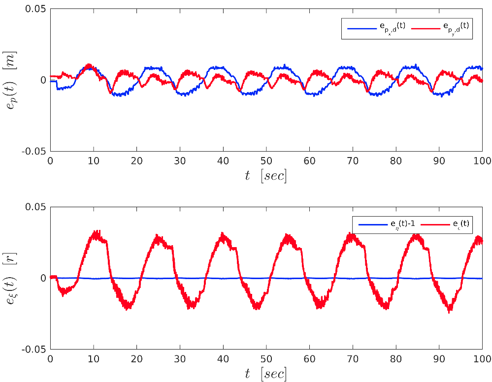
The experimental results for t=102t=10^{2}s are depicted in Fig. 3-6. In particular, the tracking of the desired object pose by the actual one is illustrated in Fig. 3. Moreover, the evolution of the errors ep​(t)e_{p}(t) and eξ​(t)e_{\xi}(t) is depicted in Fig. 4. It can be concluded from the figures that the tracking of the desired pose is achieved with some negligible oscillatory behavior that can be attributed to the deviation of the dynamics (12) from the actual coupled dynamics due to sensor noise, unmodelled friction, external disturbances and small sliding in the contact points which affects the rigidity assumption. The torque signals τi,i∈{1,2}\tau_{i},i\in\{1,2\} are pictured in Fig 5 and the task-space wrenches ui,i∈{1,2}u_{i},i\in\{1,2\} in Fig. 6. It can be seen that the proposed algorithm does not output large values for the resulting input torques and forces. A short video demonstrating the experimental setup can be found at https://youtu.be/PCnZ6C8ECFg.

Refer to caption
Figure 3: The desired (with blue) and actual (with red) pose trajectory of the object’s center of mass pO,d​(t)p_{\scriptscriptstyle O,\text{d}}(t) and pO​(t)p_{\scriptscriptstyle O}(t), respectively, for t∈[0,100]​st\in[0,100]\text{s}. Top: xx (horizontal) direction. Middle: yy (vertical) direction. Bottom: Angle ϕOz​(t)\phi_{\scriptscriptstyle O_{z}}(t) with respect to zz axis (direction perpendicular to plane xx-yy).
Refer to caption
Figure 4: The evolution of the errors ep​(t),eξ​(t),t∈[0,100]​se_{p}(t),e_{\xi}(t),t\in[0,100]\text{s}. Top: ep​(t)e_{p}(t) in xx (with blue) and yy (with red) direction. Bottom: eη​(t)−1e_{\eta}(t)-1 (with blue) and eε​(t)e_{\varepsilon}(t) (with red).
Refer to caption
Figure 5: The resulting input torques τ1​(t)\tau_{1}(t) (top) and τ2​(t)\tau_{2}(t) (bottom), t∈[0,100]​st\in[0,100]\text{s}.
Refer to caption
Figure 6: The resulting 33D task-space wrenches u1​(t)u_{1}(t) (top) and u2​(t)u_{2}(t) (bottom), t∈[0,100]​st\in[0,100]\text{s}.

6 Conclusion

We have proposed a novel control protocol for the cooperative manipulation of an object by NN robotic agents using unit quaternions and without employing any force/torque measurements. Future efforts will be devoted towards incorporating kinematic uncertainties associated with the location of the object’s center of mass, external disturbances, non-rigid grasps as well as singularity avoidance.

References

  • Aghili (2011) Aghili, F. (2011). Self-tuning cooperative control of manipulators with position/orientation uncertainties in the closed-kinematic loop. 2011 IEEE/RSJ International Conference on Intelligent Robots and Systems (IROS), 4187–4193.
  • Bai and Wen (2010) Bai, H. and Wen, J.T. (2010). Cooperative load transport: A formation-control perspective. IEEE Transactions on Robotics, 26(4), 742–750.
  • Caccavale et al. (2000) Caccavale, F., Chiacchio, P., and Chiaverini, S. (2000). Task-space regulation of cooperative manipulators. Automatica, 36(6), 879–887.
  • Caccavale et al. (2008) Caccavale, F., Chiacchio, P., Marino, A., and Villani, L. (2008). Six-dof impedance control of dual-arm cooperative manipulators. IEEE/ASME Transactions On Mechatronics, 13(5), 576–586.
  • Campa et al. (2006) Campa, R., Camarillo, K., and Arias, L. (2006). Kinematic modeling and control of robot manipulators via unit quaternions: Application to a spherical wrist. Proceedings of the IEEE Conference on Decision and Control (CDC), 6474–6479.
  • Chaimowicz et al. (2003) Chaimowicz, L., Campos, M.F.M., and Kumar, V. (2003). Hybrid systems modeling of cooperative robots. Proceedings of the IEEE International Conference on Robotics and Automation (ICRA), 3, 4086–4091.
  • Cheah et al. (2006) Cheah, C.C., Liu, C., and Slotine, J.J.E. (2006). Adaptive tracking control for robots with unknown kinematic and dynamic properties. The International Journal of Robotics Research, 25(3), 283–296.
  • Erhart and Hirche (2013) Erhart, S. and Hirche, S. (2013). Adaptive force/velocity control for multi-robot cooperative manipulation under uncertain kinematic parameters. Proceedings of the IEEE/RSJ International Conference on Intelligent Robots and Systems (IROS), 307–314.
  • Erhart and Hirche (2015) Erhart, S. and Hirche, S. (2015). Internal force analysis and load distribution for cooperative multi-robot manipulation. IEEE Transactions on Robotics, 31(5), 1238–1243.
  • Erhart and Hirche (2016) Erhart, S. and Hirche, S. (2016). Model and analysis of the interaction dynamics in cooperative manipulation tasks. IEEE Transactions on Robotics, 32(3), 672–683.
  • Erhart et al. (2013) Erhart, S., Sieber, D., and Hirche, S. (2013). An impedance-based control architecture for multi-robot cooperative dual-arm mobile manipulation. Proceedings of the IEEE/RSJ International Conference on Intelligent Robots and Systems (IROS), 315–322.
  • Ficuciello et al. (2014) Ficuciello, F., Romano, A., Villani, L., and Siciliano, B. (2014). Cartesian impedance control of redundant manipulators for human-robot co-manipulation. Proceedings of the IEEE/RSJ International Conference on Intelligent Robots and Systems (IROS), 2120–2125.
  • Gudiño-Lau et al. (2004) Gudiño-Lau, J., Arteaga, M.A., Munoz, L.A., and Parra-Vega, V. (2004). On the control of cooperative robots without velocity measurements. IEEE Transactions on Control Systems Technology, 12(4), 600–608.
  • Gueaieb et al. (2007) Gueaieb, W., Karray, F., and Al-Sharhan, S. (2007). A robust hybrid intelligent position/force control scheme for cooperative manipulators. IEEE/ASME Transactions on Mechatronics, 12(2), 109–125.
  • Heck et al. (2013) Heck, D., Kostić, D., Denasi, A., and Nijmeijer, H. (2013). Internal and external force-based impedance control for cooperative manipulation. Proceedings of the IEEE European Control Conference (ECC), 2299–2304.
  • Khatib et al. (1996) Khatib, O., Yokoi, K., Chang, K., Ruspini, D., Holmberg, R., and Casal, A. (1996). Decentralized cooperation between multiple manipulators. IEEE International Workshop on Robot and Human Communication, 183–188.
  • Kume et al. (2007) Kume, Y., Hirata, Y., and Kosuge, K. (2007). Coordinated motion control of multiple mobile manipulators handling a single object without using force/torque sensors. Proceedings of the IEEE/RSJ International Conference on Intelligent Robots and Systems (IROS), 4077–4082.
  • Li et al. (2015) Li, Z., Yang, C., Su, C.Y., Deng, S., Sun, F., and Zhang, W. (2015). Decentralized fuzzy control of multiple cooperating robotic manipulators with impedance interaction. IEEE Transactions on Fuzzy Systems, 23(4), 1044–1056.
  • Liu and Arimoto (1998) Liu, Y.H. and Arimoto, S. (1998). Decentralized adaptive and nonadaptive position/force controllers for redundant manipulators in cooperations. The International Journal of Robotics Research, 17(3), 232–247.
  • Liu et al. (1996) Liu, Y.H., Arimoto, S., and Ogasawara, T. (1996). Decentralized cooperation control: non-communication object handling. Proceedings of the IEEE Conference on Robotics and Automation (ICRA), 3, 2414–2419.
  • Mayhew et al. (2011) Mayhew, C.G., Sanfelice, R.G., and Teel, A.R. (2011). Quaternion-based hybrid control for robust global attitude tracking. IEEE Transactions on Automatic Control, 56(11), 2555–2566.
  • Murphey and Horowitz (2008) Murphey, T.D. and Horowitz, M. (2008). Adaptive cooperative manipulation with intermittent contact. Proceedings of the IEEE International Conference on Robotics and Automation (ICRA), 1483–1488.
  • Petitti et al. (2016) Petitti, A., Franchi, A., Di Paola, D., and Rizzo, A. (2016). Decentralized motion control for cooperative manipulation with a team of networked mobile manipulators. Proceedings of the IEEE International Conference on Robotics and Automation (ICRA), 441–446.
  • Ponce-Hinestroza et al. (2016) Ponce-Hinestroza, A.N., Castro-Castro, J.A., Guerrero-Reyes, H.I., Parra-Vega, V., and Olguỳn-Dỳaz, E. (2016). Cooperative redundant omnidirectional mobile manipulators: Model-free decentralized integral sliding modes and passive velocity fields. Proceedings of the IEEE International Conference on Robotics and Automation (ICRA), 2375–2380.
  • Schneider and Cannon (1992) Schneider, S.A. and Cannon, R.H. (1992). Object impedance control for cooperative manipulation: Theory and experimental results. IEEE Transactions on Robotics and Automation, 8(3), 383–394.
  • Siciliano et al. (2010) Siciliano, B., Sciavicco, L., Villani, L., and Oriolo, G. (2010). Robotics: modelling, planning and control. Springer Science & Business Media.
  • Slotine and Li (1987) Slotine, J.J.E. and Li, W. (1987). On the adaptive control of robot manipulators. The International Journal of Robotics Research, 6(3), 49–59.
  • Slotine et al. (1991) Slotine, J.J.E., Li, W., et al. (1991). Applied nonlinear control. 1. prentice-Hall Englewood Cliffs, NJ.
  • Sugar and Kumar (2002) Sugar, T.G. and Kumar, V. (2002). Control of cooperating mobile manipulators. IEEE Transactions on robotics and automation, 18(1), 94–103.
  • Szewczyk et al. (2002) Szewczyk, J., Plumet, F., and Bidaud, P. (2002). Planning and controlling cooperating robots through distributed impedance. Journal of Robotic Systems, 19(6), 283–297.
  • Tanner et al. (2003) Tanner, H.G., Loizou, S.G., and Kyriakopoulos, K.J. (2003). Nonholonomic navigation and control of cooperating mobile manipulators. IEEE Transactions on Robotics and Automation, 19(1), 53–64.
  • Tsiamis et al. (2015) Tsiamis, A., Verginis, C.K., Bechlioulis, C.P., and Kyriakopoulos, K.J. (2015). Cooperative manipulation exploiting only implicit communication. Proceedings of the IEEE/RSJ International Conference on Intelligent Robots and Systems (IROS), 864–869.
  • Wang (2017) Wang, H. (2017). Adaptive control of robot manipulators with uncertain kinematics and dynamics. IEEE Transactions on Automatic Control, 62(2), 948–954.
  • Wang and Schwager (2015) Wang, Z. and Schwager, M. (2015). Multi-robot manipulation with no communication using only local measurements. Proceedings of the IEEE Conference on Decision and Control (CDC), 380–385.
  • Wang and Schwager (2016) Wang, Z. and Schwager, M. (2016). Kinematic multi-robot manipulation with no communication using force feedback. Proceedings of the IEEE International Conference on Robotics and Automation (ICRA), 427–432.
  • Wen and Kreutz-Delgado (1992) Wen, J.T. and Kreutz-Delgado, K. (1992). Motion and force control of multiple robotic manipulators. Automatica, 28(4), 729–743.
  • Yoshikawa and Zheng (1993) Yoshikawa, T. and Zheng, X.Z. (1993). Coordinated dynamic hybrid position/force control for multiple robot manipulators handling one constrained object. The International Journal of Robotics Research, 12(3), 219–230.
  • Zribi and Ahmad (1992) Zribi, M. and Ahmad, S. (1992). Adaptive control for multiple cooperative robot arms. Proceedings of the IEEE International Conference on Decision and Control (CDC), 1392–1398.