Spin systems have the central importance, regarding the study of entanglement from the perspectives of quantum information theory (QIT) and condense matter physics. Spin as a quantum bit is a miraculous entity which has a pivotal role in the realization of quantum computers [1, 2, 3, 4]. But the main problem arises when we try to analyse the collective behavior of the infinitely large systems. Quantum renormalization group (QRG) method is an effective technique in order to address such problems, i.e. analytically in one dimension [5, 6, 7, 8, 9, 10, 11, 12, 13] and numerically in higher dimensions. In the past, different numerical techniques were used to study such systems [14, 15]. Because numerical techniques are suitable to handle the computational complexity in finding the ground states, renormalized control parameters, entanglement and critical properties in higher dimensions [16, 17, 18].

Many useful methods has been established for the study of strongly correlated quantum systems [19, 20, 21, 22]. Among these techniques, the density-matrix renormalization group method (DMRG) [23, 24, 25] is a reliable and precise numerical technique for the analysis and understanding of the low energy properties of such systems in the real space [21]. The DMRG method has been used to study the entanglement and the quantum phase transition from quantum information entropy in Heisenberg spin systems [26]. The modified DMRG scheme in a quantum system is shown to preserve the entanglement as compare to other numerical techniques [27]. Several computational methods were used to study ground states and finite temperature properties of the spin systems [28, 29].

Kadanoff’s block approach exquisitely participates in the QRG scheme by dividing the entire lattice into independent blocks whose Hamiltonian is diagnalized to obtain the lowest energy degenerate states which are further used for the construction of the renormalized Hilbert space in the lower dimensions [30]. Recently, we extended the application of Kadanoffs block approach from the one dimension to the two dimensional Hisenberg $XY$ model [31] . From the previous study[31], we realize that the symetrical extension to the three-dimensional spin system is quite possible and is presented here. Where we developed the two-dimensional five-spins Kadanoff block from the one-dimensional three-spins kadanoff block. In this study the progression from the two-dimensional five-spins Kadanoff block to the three-dimensional seven-spins Kadanoff block is presented.

The study of quantum correlations in the spin systems through the QRG reflects both quantum information properties as well as critical properties of the system [31, 5, 10, 6, 29, 32, 33]. The ground-state spin entanglement in d-dimensional bipartite lattice of the $XXZ$ moel is studied [34], where bipartite concurrence shows similar qualitative behavior. It reaches to maximum value at the critical point and it can be seen that this maximum value is smaller in three dimensions as compared to its two-dimensional counterpart. Likewise scenario can be seen for the qualitative and the quantitative behavior of the concurrence in the $XY$ model, as we go from the lower to higher dimensions [10, 31]. It is the monogamy that limits the entanglement shared among the number of neighbor sites [19]. Similarly, the symmetry of the Hamiltonian predicts that the magnitude of the entanglement may further reduce in three dimensions due to increase in the interactions. Moreover, the monogamy is responsible for achieving the critical point more rapidly, as less QRG iterations are required in higher dimensions [31]. This critical phenomenon is described by the behavior of the ground state entanglement as the system size increases.

In the study presented here, a numerical approach is adopted for the RG evolution of the spin -1/2 $XY$ model for all the spatial dimensions. Symmetries of the system allow us to span the spin lattices via Kadanoff’s block approach by considering three, five and seven spins in one, two and three-dimensions respectively (Fig. 1.), which is necessary in the context of obtaining degenerate ground states for the $XY$ model. In this way, the entire lattice is comprised of blocks, where the each block interacts with all its nearest neighbors through the interblock interactions (Fig. 2.). We compute the lowest energy eigenvalues of each Kadanoff block and construct the density matrix from the ground states of the system. We choose the geometric average of the bipartite concurrence as the entanglement measure because each interblock spin-spin interaction can be seen as bipartite interaction (Fig. 2.). Here, it is worth mentioning that the reduced density matrices for the different bipartite interblock spin-spin interactions in two and three dimensions are exactly same which is the manifestation of the symmetries possessed by the model in all dimensions. Quantitatively, it is found that for a given spatial dimension, the result obtained from the geometric average of the bipartite concurrences of possible interblock spin-spin interactions is equal to the any of the single bipartite concurrence. The evolution of the entanglement displays the comparative behavior in this study. Finally, we discuss the scaling behavior by observing the absolute maximum value of the derivative of the concurrence and by measuring the entanglement exponent which portray that how the system approaches critical point in all dimensions.

The QRG technique is a method in which lattice size is reduced in each step of iteration and reaches a situation where control parameters sustain the previous renormalized value. Thus the single block with renormalized coupling constants represents an infinitely large system. The construction of this block is obtained by using well defined Kadanoff’s block approach [35, 36]. We consider blocks of three, five and seven spins in one, two and three dimensions respectively (Fig. 1.) to obtain the effective Hamiltonian which has similar structure as that of the original Hamiltonian. From the previous studies of the $XY$ model [10, 11, 31], it is found that in the renormalization process, the projection operator constructed from the degenerate ground states of the block works well for obtaining the effective Hamiltonian in the renormalized Hilbert space of spin -1/2 particle. The degenerate ground eigenstates can only be obtained if we consider the blocks containing odd number of spins in any spatial dimensions. In the construction of Kadanoff’s block we make symmetrical transformation from the lower to higher dimensions with respect to the central spin of the block, i.e., in two dimensions two nearest neighbors are added in $y$-direction while in three dimensions further two nearest neighbors are added in the the $z$-direction to the central spin of the one-dimensional Kaddanoff’s block (Fig. 1.).

The generalized form of the Hamiltonian in $d$-dimensions, for $\prod\limits_{d}N_{d},$ spins where $N_{d}=N$ with $d=1,2,3$ for one, two and three dimensions respectively, can be represented by,

	$\displaystyle H_{d}$	$\displaystyle=$	$\displaystyle\frac{J}{4}\prod\limits_{p=1}^{d}S_{p}[\sum_{q=x,y}(1+\gamma_{q})(c_{1}\sigma_{c_{1}i,c_{2}j,c_{3}k}^{q}\sigma_{c_{1}(i+1),c_{2}j,c_{3}k}^{q}$		(1)
			$\displaystyle+c_{2}\sigma_{c_{1}i,c_{2}j,c_{3}k}^{q}\sigma_{c_{1}i,c_{2}(j+1),c_{3}k}^{q}+c_{3}\sigma_{c_{1}i,c_{2}j,c_{3}k}^{q}\sigma_{c_{1}i,c_{2}j,c_{3}(k+1)}^{q})],$

Where, $\gamma_{x}=\gamma,\gamma_{y}=-\gamma,S_{p}=\sum_{r=1}^{N_{d}}$ with $r=i,j$ and $k$ for $p=1,2$ and $3$ respectively along with the constants $c_{1}=1,c_{2}=(d-1)/2^{((d-1)(d-2)/2)}$ and $c_{3}=(d-1)(d-2)/2$. $\sigma^{x}$ and $\sigma^{y}$ are the Pauli spin matrices where as $J$ and $\gamma$ represent the coupling strength and anisotropic parameter respectively. The sign of the coupling strength $J$ determines whether the model lies in antiferromagnetic or ferromagnetic regime. We use the positive value of $J$ which corresponds to antiferromagnetic case. However, the sign of $j$ does not effect the results. The quantum fluctuations are driven by the values of control parameter $\gamma$. Different values of $\gamma$ reduce the model to different classes. i.e., at $\gamma=1$ the system is Ising, for $\gamma=0$ it is $XX$ and for all other values it is Ising universal class.

For renormalization process, we split the original Hamiltonian $H_{d}$ in to two parts, the block $H_{d}^{B}$ and the interblock $H_{d}^{BB}$ [5, 7, 8, 10, 11, 31]. The effective Hamiltonian $H_{d}^{eff}$ is obtained from the $\pi^{\dagger}H_{d}\pi$, where $\pi=\left|\Uparrow\right\rangle\left\langle\phi_{0}^{1}\right|+\left|\Downarrow\right\rangle\left\langle\phi_{0}^{2}\right|$ is the projection operator obtained by projecting the $2^{n}$ (where $n=3,5,7$ for one , two and three dimensions respectively) dimensional degenerate ground states $\left|\phi_{0}^{1}\right\rangle$ and $\left|\phi_{0}^{2}\right\rangle$ of the block on spin-$1/2$ qubits $\left|\Uparrow\right\rangle$ and $\left|\Downarrow\right\rangle$ resulting in a projection operator in $2$-dimensional Hilbert space. Finally, we obtained the renormalized numerical values of the coupling constant $j^{\prime}$ and the anisotropy parameter $\gamma^{\prime}$ from the effective Hamiltonian. Some numerical values of $\gamma$ for different RG steps in the real-space are given in TABLE.1. The solution for $\gamma=\gamma^{\prime}$ can be found by plotting $\gamma^{\prime}$ against $\gamma$ for the first RG step iteration (Fig.3.), which shows that the model attains two different phases for $\gamma\rightarrow-1$ or $+1$ referring to Ising like phase and $\gamma\rightarrow 0,$ to spin fluid phase suggesting that there lies a phase boundary between these two phases. We can see from the plot (Fig.3.) that the phase boundary is more prominent in higher dimensions even in the first RG iteration compared to the corresponding system in lower dimensions. Hence the model demands less number of RG iterations in higher dimensions to reach at the critical point.

To perform the comparative study of the $XY$-model in the real space by the QRG technique, we choose the concurrence as the entanglement measure [37]. In one dimension, bipartite interblock spin-spin interaction exists through out the spin chain, while in higher dimensions many bipartite interblock interactions are present. From this perspective it may be appropriate to use the geometric average of the bipartite concurrences as a generalized criterion for the entanglement study. Further we find that the value of each bipartite concurrence for any particular iteration is same and equal to the geometric average of the bipartite concurrences. Therefore, keeping in view this scenario, we can use a single bipartite concurrence as the entanglement measure. The bipartite concurrence $C_{ij}$ for $i^{th}$ and $j^{th}$ nearest neighbor spins obtained from reduced density matrix $\rho_{ij}$ is given as

$$C_{ij}=\max[\sqrt{\lambda_{ij,4}}-\sqrt{\lambda_{ij,3}}-\sqrt{\lambda_{ij,2}}-\sqrt{\lambda_{ij,1}},0],$$

(2)

where $\lambda_{ij,k}$ for $(k=1,2,3,4)$ are the eigenvalues of matrix $\rho_{ij}\tilde{\rho}_{ij}$ with $\tilde{\rho}_{ij}=(\sigma_{i}^{y}\otimes\sigma_{j}^{y})$ $\rho_{ij}^{\ast}(\sigma_{i}^{y}\otimes\sigma_{j}^{y})$ and $\lambda_{ij,4}>\lambda_{ij,3}>\lambda_{ij,2}>\lambda$. The reduced density matrix $\rho_{ij}$ for the spins interaction $i$ and $j$ is constructed by taking the marginal partial traces of the total density matrix $\rho$ where, $\rho=\left|\phi_{0}^{1}\right\rangle\left\langle\phi_{0}^{1}\right|$ is obtained from any of the degenerate ground state of the Hamiltonian.

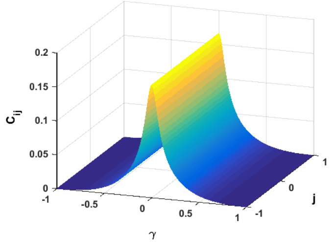
The numerical results of the concurrence $C_{ij}$ are plotted against the anisotropy parameter $\gamma$ (Fig. 4.) for the first three RG iterations of the spin-$1/2$ $XY$ model in all dimensions. The concurrence shows similar qualitative behavior but smaller in magnitude in higher dimensions as compare to lower dimensions. At $\gamma=0$, the concurrence attains maximum values which are $0.5$, $0.25$ and $0.167$ in one, two and three dimensions respectively. We find that the maximum value of concurrence decreases by the factor of $1/n$ $(n=2,3)$ compared to the one-dimensional case. It can be interpreted that the concurrence decreases with the increase in monogamy in the higher dimensions. In all dimensions, in the final iteration the system reaches thermodynamic limit and the concurrence acquires two fixed values, one non zero at the critical point ($\gamma=0)$ favoring long range disordered phase and the other at $\gamma\neq 0$, where the concurrence is zero and the system corresponds to a dominant ordered phase. The phenomenon of phase transition for the $XY$ model in the real space can also be seen through the non analytic behavior of the concurrence where the derivative of the concurrence shows the discontinuity at the critical point (Fig. 4.). Whereas the concurrence itself remains continuous as the system size becomes infinitely large. Such phase transitions are named as the second-order QPT.

The detail analysis of the entanglement as a resource for exploring the critical phenomenon in the one-dimensional $XY$ model has been done in Ref. [32, 38]. It was cojectured that the system is maximally entangled at the critical point corresponding to the delocalized state, where the correlations exist on all length scales, in contrast to the situation away from the critical point favoring the exponential decay of the correlations as a function of sites separation [39]. Our results depict similar behavior for the entanglement in the vicinity of the critical point even in all the spatial dimensions. These numerical results of entanglement are also supported by the previous analytical results of $1D$ and $2D$ $XY$ model [10, 31]. In Ref. [32, 38], the transverse Ising model was considered as a special case of the $XY$ model for anisotropy parameter $\gamma=1$. In the limiting case of the transverse Ising model, where the effect of external field is very small the value of entanglement approaches zero conforming to our result of Ising phase for $\gamma=\pm 1$. The degenerate ground states at $\gamma=1$ for $XY$ model for the second step RG iteration are given in the appendix.

The emergence of singularity by the divergence of the derivative can be probed by investigating the scaling behavior which relates maximum/minimum of the derivative of entanglement with the system size. From the comparative plots (Fig. 5.), it is observed that in each dimension, the derivative of the concurrence shows linear behavior on the logarithmic scale but the slope increases with increasing the dimensionality of the system. Which indicates that the system diverges rapidly in higher dimensions. To analyze that how fast the system reaches the transition point, the $\ln(\gamma_{c}-\gamma_{m})$ is plotted against the $\ln(N)$ (Fig.6.). The value of the entanglement exponent $\theta$ can be found from the relation $\gamma_{m}=\gamma_{c}-N^{-\theta}$, which are are $0.73$, $1.48$ and $1.60$ for one, two and three dimensions respectively. It can be seen that the entanglement exponent is highest in three dimensions, which corresponds to smaller correlation length, supporting the idea that it reaches the thermodynamic limit rapidly and acquires phase transition in less number of RG iterations. It is worth mentioning that the divergence of the derivative of the concurrence in the vicinity of the quantum phase transition point was investigated in one-dimensional $XY$ model with different lattice sizes in Ref. [32] and with QRG technique in Ref. [10, 11, 31]. Complying to these studies, the entanglement in our study, also obeys the scaling behavior near the critical point.

The QRG in the real-space for the spin -$1/2$ $XY$ model is achieved. We see that for the concurrence as the entanglement measure, the system shows similar qualitative behavior in all dimensions, which is the manifestation of the symmetric interactions present in the model. But the maximum value of the entanglement in two and three dimensional $XY$ model is decreased by the factor of $1/n$, where $n=2,3$, with reference to the one-dimensional case. The reduction in the peak value is due to the increase in the monogamy of the spins interactions. Our results are consistent with the previous studies of the one and two-dimensional $XY$ model. This study will be helpful in understanding the behavior of the entanglement and the critical phenomenon for different types of complex spin systems in real-space.

This work is partly supported by the HIGHER EDUCATION COMMISSION, PAKISTAN under the Indigenous Ph.D. Fellowship Scheme.

The expression for degenerate ground state eigenvectors $|\phi(1)\rangle$ and $|\phi(2)\rangle$ of the $1D$, $2D$ and $3D$ $XY$ model at $\gamma=1$ corresponding to the Ising class are given below;

$\displaystyle|\phi_{1}\rangle^{1D}=-0.5|\uparrow\uparrow\uparrow\rangle+0.5|\uparrow\downarrow\downarrow\rangle-0.5|\downarrow\uparrow\downarrow\rangle+0.5|\downarrow\downarrow\uparrow\rangle$

$\displaystyle|\phi_{2}\rangle^{1D}=-0.5|\uparrow\uparrow\downarrow\rangle+0.5|\uparrow\downarrow\uparrow\rangle-0.5|\downarrow\uparrow\uparrow\rangle+0.5|\downarrow\downarrow\downarrow\rangle$

	$\displaystyle|\phi_{1}\rangle^{2D}=-0.25|\uparrow\uparrow\uparrow\uparrow\downarrow\rangle-0.25|\uparrow\uparrow\uparrow\downarrow\uparrow\rangle-0.25|\uparrow\uparrow\downarrow\uparrow\uparrow\rangle-0.25|\uparrow\uparrow\downarrow\downarrow\downarrow\rangle-0.25|\uparrow\downarrow\uparrow\uparrow\uparrow\rangle-0.25|\uparrow\downarrow\uparrow\downarrow\downarrow\rangle-0.25|\uparrow\downarrow\downarrow\uparrow\downarrow\rangle-$
	$\displaystyle 0.25|\uparrow\downarrow\downarrow\downarrow\uparrow\rangle+0.25|\downarrow\uparrow\uparrow\uparrow\uparrow\rangle+0.25|\downarrow\uparrow\uparrow\downarrow\downarrow\rangle+0.25|\downarrow\uparrow\downarrow\uparrow\downarrow\rangle+0.25|\downarrow\uparrow\downarrow\downarrow\uparrow\rangle+0.25|\downarrow\downarrow\uparrow\uparrow\downarrow\rangle+0.25|\downarrow\downarrow\uparrow\downarrow\uparrow\rangle+$
	$\displaystyle 0.25|\downarrow\downarrow\downarrow\uparrow\uparrow\rangle+0.25|\downarrow\downarrow\downarrow\downarrow\downarrow\rangle$

	$\displaystyle|\phi_{2}\rangle^{2D}=0.25|\uparrow\uparrow\uparrow\uparrow\uparrow\rangle+0.25|\uparrow\uparrow\uparrow\downarrow\downarrow\rangle+0.25|\uparrow\uparrow\downarrow\uparrow\downarrow\rangle+0.25|\uparrow\uparrow\downarrow\downarrow\uparrow\rangle+0.25|\uparrow\downarrow\uparrow\uparrow\downarrow\rangle+0.25|\uparrow\downarrow\uparrow\downarrow\uparrow\rangle+0.25|\uparrow\downarrow\downarrow\uparrow\uparrow\rangle+$
	$\displaystyle 0.25|\uparrow\downarrow\downarrow\downarrow\downarrow\rangle-0.25|\downarrow\uparrow\uparrow\uparrow\downarrow\rangle-0.25|\downarrow\uparrow\uparrow\downarrow\uparrow\rangle-0.25|\downarrow\uparrow\downarrow\uparrow\uparrow\rangle-0.25|\downarrow\uparrow\downarrow\downarrow\downarrow\rangle-0.25|\downarrow\downarrow\uparrow\uparrow\uparrow\rangle-0.25|\downarrow\downarrow\uparrow\downarrow\downarrow\rangle-$
	$\displaystyle 0.25|\downarrow\downarrow\downarrow\uparrow\downarrow\rangle-0.25|\downarrow\downarrow\downarrow\downarrow\uparrow\rangle$

	$\displaystyle|\phi_{1}\rangle^{3D}=0.125|\uparrow\uparrow\uparrow\uparrow\uparrow\uparrow\uparrow\rangle+0.125|\uparrow\uparrow\uparrow\uparrow\uparrow\downarrow\downarrow\rangle+0.125|\uparrow\uparrow\uparrow\uparrow\downarrow\uparrow\downarrow\rangle+0.125|\uparrow\uparrow\uparrow\uparrow\downarrow\downarrow\uparrow\rangle+0.125|\uparrow\uparrow\uparrow\downarrow\uparrow\uparrow\downarrow\rangle+0.125|\uparrow\uparrow\uparrow\downarrow\uparrow\downarrow\uparrow\rangle+$
	$\displaystyle 0.125|\uparrow\uparrow\uparrow\downarrow\downarrow\uparrow\uparrow\rangle+0.125|\uparrow\uparrow\uparrow\downarrow\downarrow\downarrow\downarrow\rangle+0.125|\uparrow\uparrow\downarrow\uparrow\uparrow\uparrow\downarrow\rangle+0.125|\uparrow\uparrow\downarrow\uparrow\uparrow\downarrow\uparrow\rangle+0.125|\uparrow\uparrow\downarrow\uparrow\downarrow\uparrow\uparrow\rangle+0.125|\uparrow\uparrow\downarrow\uparrow\downarrow\downarrow\downarrow\rangle+$
	$\displaystyle 0.125|\uparrow\uparrow\downarrow\downarrow\uparrow\uparrow\uparrow\rangle+0.125|\uparrow\uparrow\downarrow\downarrow\uparrow\downarrow\downarrow\rangle+0.125|\uparrow\uparrow\downarrow\downarrow\downarrow\uparrow\downarrow\rangle+0.125|\uparrow\uparrow\downarrow\downarrow\downarrow\downarrow\uparrow\rangle+0.125|\uparrow\downarrow\uparrow\uparrow\uparrow\uparrow\downarrow\rangle+0.125|\uparrow\downarrow\uparrow\uparrow\uparrow\downarrow\uparrow\rangle+$
	$\displaystyle 0.125|\uparrow\downarrow\uparrow\uparrow\downarrow\uparrow\uparrow\rangle+0.125|\uparrow\downarrow\uparrow\uparrow\downarrow\downarrow\downarrow\rangle+0.125|\uparrow\downarrow\uparrow\downarrow\uparrow\uparrow\uparrow\rangle+0.125|\uparrow\downarrow\uparrow\downarrow\uparrow\downarrow\downarrow\rangle+0.125|\uparrow\downarrow\uparrow\downarrow\downarrow\uparrow\downarrow\rangle+0.125|\uparrow\downarrow\uparrow\downarrow\downarrow\downarrow\uparrow\rangle+$
	$\displaystyle 0.125|\uparrow\downarrow\downarrow\uparrow\uparrow\uparrow\uparrow\rangle+0.125|\uparrow\downarrow\downarrow\uparrow\uparrow\downarrow\downarrow\rangle+0.125|\uparrow\downarrow\downarrow\uparrow\downarrow\uparrow\downarrow\rangle+0.125|\uparrow\downarrow\downarrow\uparrow\downarrow\downarrow\uparrow\rangle+0.125|\uparrow\downarrow\downarrow\downarrow\uparrow\uparrow\downarrow\rangle+0.125|\uparrow\downarrow\downarrow\downarrow\uparrow\downarrow\uparrow\rangle+$
	$\displaystyle 0.125|\uparrow\downarrow\downarrow\downarrow\downarrow\uparrow\uparrow\rangle+0.125|\uparrow\downarrow\downarrow\downarrow\downarrow\downarrow\downarrow\rangle-0.125|\downarrow\uparrow\uparrow\uparrow\uparrow\uparrow\downarrow\rangle-0.125|\downarrow\uparrow\uparrow\uparrow\uparrow\downarrow\uparrow\rangle-0.125|\downarrow\uparrow\uparrow\uparrow\downarrow\uparrow\uparrow\rangle-0.125|\downarrow\uparrow\uparrow\uparrow\downarrow\downarrow\downarrow\rangle-$
	$\displaystyle 0.125|\downarrow\uparrow\uparrow\downarrow\uparrow\uparrow\uparrow\rangle-0.125|\downarrow\uparrow\uparrow\downarrow\uparrow\downarrow\downarrow\rangle-0.125|\downarrow\uparrow\uparrow\downarrow\downarrow\uparrow\downarrow\rangle-0.125|\downarrow\uparrow\uparrow\downarrow\downarrow\downarrow\uparrow\rangle-0.125|\downarrow\uparrow\downarrow\uparrow\uparrow\uparrow\uparrow\rangle-0.125|\downarrow\uparrow\downarrow\uparrow\uparrow\downarrow\downarrow\rangle-$
	$\displaystyle 0.125|\downarrow\uparrow\downarrow\uparrow\downarrow\uparrow\downarrow\rangle-0.125|\downarrow\uparrow\downarrow\uparrow\downarrow\downarrow\uparrow\rangle-0.125|\downarrow\uparrow\downarrow\downarrow\uparrow\uparrow\downarrow\rangle-0.125|\downarrow\uparrow\downarrow\downarrow\uparrow\downarrow\uparrow\rangle-0.125|\downarrow\uparrow\downarrow\downarrow\downarrow\uparrow\uparrow\rangle-0.125|\downarrow\uparrow\downarrow\downarrow\downarrow\downarrow\downarrow\rangle-$
	$\displaystyle 0.125|\downarrow\downarrow\uparrow\uparrow\uparrow\uparrow\uparrow\rangle-0.125|\downarrow\downarrow\uparrow\uparrow\uparrow\downarrow\downarrow\rangle-0.125|\downarrow\downarrow\uparrow\uparrow\downarrow\uparrow\downarrow\rangle-0.125|\downarrow\downarrow\uparrow\uparrow\downarrow\downarrow\uparrow\rangle-0.125|\downarrow\downarrow\uparrow\downarrow\uparrow\uparrow\downarrow\rangle-0.125|\downarrow\downarrow\uparrow\downarrow\uparrow\downarrow\uparrow\rangle-$
	$\displaystyle 0.125|\downarrow\downarrow\uparrow\downarrow\downarrow\uparrow\uparrow\rangle-0.125|\downarrow\downarrow\uparrow\downarrow\downarrow\downarrow\downarrow\rangle-0.125|\downarrow\downarrow\downarrow\uparrow\uparrow\uparrow\downarrow\rangle-0.125|\downarrow\downarrow\downarrow\uparrow\uparrow\downarrow\uparrow\rangle-0.125|\downarrow\downarrow\downarrow\uparrow\downarrow\uparrow\uparrow\rangle-0.125|\downarrow\downarrow\downarrow\uparrow\downarrow\downarrow\downarrow\rangle-$
	$\displaystyle 0.125|\downarrow\downarrow\downarrow\downarrow\uparrow\uparrow\uparrow\rangle-0.125|\downarrow\downarrow\downarrow\downarrow\uparrow\downarrow\downarrow\rangle-0.125|\downarrow\downarrow\downarrow\downarrow\downarrow\uparrow\downarrow\rangle-0.125|\downarrow\downarrow\downarrow\downarrow\downarrow\downarrow\uparrow\rangle$

	$\displaystyle|\phi_{2}\rangle^{3D}=-0.125|\uparrow\uparrow\uparrow\uparrow\uparrow\uparrow\downarrow\rangle-0.125|\uparrow\uparrow\uparrow\uparrow\uparrow\downarrow\uparrow\rangle-0.125|\uparrow\uparrow\uparrow\uparrow\downarrow\uparrow\uparrow\rangle-0.125|\uparrow\uparrow\uparrow\uparrow\downarrow\downarrow\downarrow\rangle-0.125|\uparrow\uparrow\uparrow\downarrow\uparrow\uparrow\uparrow\rangle-0.125|\uparrow\uparrow\uparrow\downarrow\uparrow\downarrow\downarrow\rangle-$
	$\displaystyle 0.125|\uparrow\uparrow\uparrow\downarrow\downarrow\uparrow\downarrow\rangle-0.125|\uparrow\uparrow\uparrow\downarrow\downarrow\downarrow\uparrow\rangle-0.125|\uparrow\uparrow\downarrow\uparrow\uparrow\uparrow\uparrow\rangle-0.125|\uparrow\uparrow\downarrow\uparrow\uparrow\downarrow\downarrow\rangle-0.125|\uparrow\uparrow\downarrow\uparrow\downarrow\uparrow\downarrow\rangle-0.125|\uparrow\uparrow\downarrow\uparrow\downarrow\downarrow\uparrow\rangle-$
	$\displaystyle 0.125|\uparrow\uparrow\downarrow\downarrow\uparrow\uparrow\downarrow\rangle-0.125|\uparrow\uparrow\downarrow\downarrow\uparrow\downarrow\uparrow\rangle-0.125|\uparrow\uparrow\downarrow\downarrow\downarrow\uparrow\uparrow\rangle-0.125|\uparrow\uparrow\downarrow\downarrow\downarrow\downarrow\downarrow\rangle-0.125|\uparrow\downarrow\uparrow\uparrow\uparrow\uparrow\uparrow\rangle-0.125|\uparrow\downarrow\uparrow\uparrow\uparrow\downarrow\downarrow\rangle-$
	$\displaystyle 0.125|\uparrow\downarrow\uparrow\uparrow\downarrow\uparrow\downarrow\rangle-0.125|\uparrow\downarrow\uparrow\uparrow\downarrow\downarrow\uparrow\rangle-0.125|\uparrow\downarrow\uparrow\downarrow\uparrow\uparrow\downarrow\rangle-0.125|\uparrow\downarrow\uparrow\downarrow\uparrow\downarrow\uparrow\rangle-0.125|\uparrow\downarrow\uparrow\downarrow\downarrow\uparrow\uparrow\rangle-0.125||\uparrow\downarrow\uparrow\downarrow\downarrow\downarrow\downarrow\rangle-$
	$\displaystyle 0.125|\uparrow\downarrow\downarrow\uparrow\uparrow\uparrow\downarrow\rangle-0.125|\uparrow\downarrow\downarrow\uparrow\uparrow\downarrow\uparrow\rangle-0.125|\uparrow\downarrow\downarrow\uparrow\downarrow\uparrow\uparrow\rangle-0.125|\uparrow\downarrow\downarrow\uparrow\downarrow\downarrow\downarrow\rangle-0.125|\uparrow\downarrow\downarrow\downarrow\uparrow\uparrow\uparrow\rangle-0.125|\uparrow\downarrow\downarrow\downarrow\uparrow\downarrow\downarrow\rangle-$
	$\displaystyle 0.125|\uparrow\downarrow\downarrow\downarrow\downarrow\uparrow\downarrow\rangle-0.125|\uparrow\downarrow\downarrow\downarrow\downarrow\downarrow\uparrow\rangle+0.125|\downarrow\uparrow\uparrow\uparrow\uparrow\uparrow\uparrow\rangle+0.125|\downarrow\uparrow\uparrow\uparrow\uparrow\downarrow\downarrow\rangle+0.125|\downarrow\uparrow\uparrow\uparrow\downarrow\uparrow\downarrow\rangle+0.125|\downarrow\uparrow\uparrow\uparrow\downarrow\downarrow\uparrow\rangle+$
	$\displaystyle 0.125|\downarrow\uparrow\uparrow\downarrow\uparrow\uparrow\downarrow\rangle+0.125|\downarrow\uparrow\uparrow\downarrow\uparrow\downarrow\uparrow\rangle+0.125|\downarrow\uparrow\uparrow\downarrow\downarrow\uparrow\uparrow\rangle+0.125|\downarrow\uparrow\uparrow\downarrow\downarrow\downarrow\downarrow\rangle+0.125|\downarrow\uparrow\downarrow\uparrow\uparrow\uparrow\downarrow\rangle+0.125|\downarrow\uparrow\downarrow\uparrow\uparrow\downarrow\uparrow\rangle+$
	$\displaystyle 0.125|\downarrow\uparrow\downarrow\uparrow\downarrow\uparrow\uparrow\rangle+0.125|\downarrow\uparrow\downarrow\uparrow\downarrow\downarrow\downarrow\rangle+0.125|\downarrow\uparrow\downarrow\downarrow\uparrow\uparrow\uparrow\rangle+0.125|\downarrow\uparrow\downarrow\downarrow\uparrow\downarrow\downarrow\rangle+0.125|\downarrow\uparrow\downarrow\downarrow\downarrow\uparrow\downarrow\rangle+0.125|\downarrow\uparrow\downarrow\downarrow\downarrow\downarrow\uparrow\rangle+$
	$\displaystyle 0.125|\downarrow\downarrow\uparrow\uparrow\uparrow\uparrow\downarrow\rangle+0.125|\downarrow\downarrow\uparrow\uparrow\uparrow\downarrow\uparrow\rangle+0.125|\downarrow\downarrow\uparrow\uparrow\downarrow\uparrow\uparrow\rangle+0.125|\downarrow\downarrow\uparrow\uparrow\downarrow\downarrow\downarrow\rangle+0.125|\downarrow\downarrow\uparrow\downarrow\uparrow\uparrow\uparrow\rangle+0.125|\downarrow\downarrow\uparrow\downarrow\uparrow\downarrow\downarrow\rangle+$
	$\displaystyle 0.125|\downarrow\downarrow\uparrow\downarrow\downarrow\uparrow\downarrow\rangle+0.125|\downarrow\downarrow\uparrow\downarrow\downarrow\downarrow\uparrow\rangle+0.125|\downarrow\downarrow\downarrow\uparrow\uparrow\uparrow\uparrow\rangle+0.125|\downarrow\downarrow\downarrow\uparrow\uparrow\downarrow\downarrow\rangle+0.125|\downarrow\downarrow\downarrow\uparrow\downarrow\uparrow\downarrow\rangle+0.125|\downarrow\downarrow\downarrow\uparrow\downarrow\downarrow\uparrow\rangle+$
	$\displaystyle 0.125|\downarrow\downarrow\downarrow\downarrow\uparrow\uparrow\downarrow\rangle+0.125|\downarrow\downarrow\downarrow\downarrow\uparrow\downarrow\uparrow\rangle+0.125|\downarrow\downarrow\downarrow\downarrow\downarrow\uparrow\uparrow\rangle+0.125|\downarrow\downarrow\downarrow\downarrow\downarrow\downarrow\downarrow\rangle$

Both the degenerate eigenvectors are normalized and orthogonal i.e., $\langle\phi_{i}|\phi_{j}\rangle=\delta_{ij}$ where $\delta_{ij}$ is the Kronecker delta function.

References

- [1] M. A. Nielsen and I. L. Chuang, Quantum Computation and Quantum Communication (Cambridge University Press, Cambridge, 2000).
- [2] DiVincenzo, David P. Science 270.5234 (Oct 13, 1995): 255.
- [3] I. M. Georgescu, S. Ashhab and F. Nori, Rev. Mod. Phys. 86, 153 (2014).
- [4] A. Galindo and M. A. Martin-Delgado, Rev. Mod. Phys. 74, 347 (2002).
- [5] M. Kargarian, R. Jafari, and A. Langari, Phys. Rev. A 76, 060304(R) (2007).
- [6] A. Langari, Phys. Rev. B 69, 100402(R) (2004)
- [7] M. Kargarian, R. Jafari, and A. Langari, Phys. Rev. A 77, 032346 (2008).
- [8] M. Kargarian, R. Jafari, and A. Langari, Phys. Rev. A 79, 042319 (2009).
- [9] R. Jafari and A. Langari, Physica A 364, 213 (2006).
- [10] Fu-Wu Ma, Sheng-Xin Liu, and Xiang-Mu Kong, Phys. Rev. A 83, 062309 (2011).
- [11] Fu-Wu Ma, Sheng-Xin Liu, and Xiang-Mu Kong, Phys. Rev. A 84, 042302 (2011).
- [12] X. M. Liu, W. W. Cheng and J. -M. Liu, Sci. Rep. 6, 19359 (2016).
- [13] Sun, W., Shi, J., Wang, D. et al. Quantum Inf Process (2016) 15: 245
- [14] Syljuåsen, O., 2003a, Phys. Lett. A 322, 25 (2004).
- [15] Syljuåsen, O., 2003b, Phys. Rev. A 68, 060301 (R) (2003).
- [16] G. Evenbly and G. Vidal, Phys. Rev. Lett. 102, 180406 (2009).
- [17] G. Vidal, Phys. Rev. Lett. 99, 220405 (2007).
- [18] Y. Xu, X. Kong, Z. Liu and C. Wang, Physica A 446, 217 (2016).
- [19] L. Amico, R. Fazio, A. Osterloh, and V. Vedral, Rev. Mod. Phys. 80, 517 (2008).
- [20] K. G. Wilson, Rev. Mod. Phys. 47, 773 (1975).
- [21] U. Schollwöck, Rev. Mod. Phys. 77, 259 (2005).
- [22] S. Gu, G. Tian and H. Lin, New J. Phys. 8, 61 (2006).
- [23] S. R. White, Phys. Rev. Lett. 69, 2863 (1992).
- [24] S. R. White and R. M. Noack, Phys. Rev. Lett. 68, 3487 (1992).
- [25] S. R. White, Phys. Rev. B 48, 10345 (1993).
- [26] O. Legeza, R. M. Noack, J. Solyom, and L. Tincani, Applications of Quantum Information in the Density-Matrix Renormalization Group, Vol. 739 (Springer, Berlin, 2008).
- [27] T. J. Osborne and M. A. Neilsen, Quantum Inf Process (2002) 1: 45
- [28] A. W. Sandvik, AIP Conference Proceedings 1297, 135 (2010).
- [29] G. Vidal, J. I. Latorre, E.Rico and A. Kitaev, Phys. Rev. Lett. 90, 227902 (2003).
- [30] J. Gonzālez, M. A. Martin Deigado, G. Sierra and A. H. Vozmediano, Quantum Electron Liquid and High-Tc Super Conductivity, edited by H. Araki et al., Lecture Notes in Physics Vo38. (Springer, Berlin, 1995), Chap. 11.
- [31] M. Usman, Asif Ilyas and Khalid Khan, Phys. Rev. A 92, 032327 (2015)
- [32] A. Osterloh, L. Amico, G. Falci and R. Fazio, Nature (London) 416, 608 (2002).
- [33] M. Zhong and P. Tong, J. Phys. A: Math. Theor. 43, 505302 (2010).
- [34] Shi-Jian Gu, Guang-Shan Tian and Hai-Qing Lin, Phys. Rev. A 71, 052322 (2005)
- [35] G. Sierra and M. A. Martin-Delgado, in Strongly Correlated Magnetic and Superconducting Systems, edited by H. Araki et al., Lecture Notes in Physics Vol. 478 (Springer, Berlin, 1997).
- [36] M. A. Martin-Delgado and G. Sierra, Int. J. Mod. Phys. A 11, 3145 (1996).
- [37] W. K. Wootters, Phys. Rev. Lett. 80, 2245 (1998).
- [38] T. J. Osborne and M. A. Neilsen, Phys. Rev. A 66, 032110 (2002)
- [39] S. Sachdev, Quantum Phase Transitions (Cambridge University Press, Cambridge, 1999).