CERN-TH-2016-212
The Slab Method to Measure the Topological SusceptibilityThanks: We
thank Stephan Dürr, Massimo D’Elia and
Marc Wagner for helpful discussions. This work was supported
by the Mexican Consejo Nacional de Ciencia y
Tecnología (CONACYT) through projects CB-2010/155905 and
CB-2013/222812, by DGAPA-UNAM, grant IN107915, and by the
Helmholtz International Center for FAIR within the
framework of the LOEWE program launched by the State of Hesse.
A.D. acknowledges support by the Emmy Noether Programme
of the DFG (German Research Foundation), grant WA 3000/1-1. The
computations were performed on the cluster of ICN/UNAM, and
on the LOEWE-CSC and FUCHS-CSC high-performance
computer of Frankfurt University.
Abstract:
In simulations of a model with topological sectors, algorithms which proceed in small update steps tend to get stuck in one sector, especially on fine lattices. This distorts the numerical results; in particular it is not straightforward to measure the topological susceptibility . We test a method to measure even if configurations from only one sector are available. It is based on the topological charges in sub-volumes, which we denote as “slabs”. This enables the evaluation of , as we demonstrate with numerical results for non-linear -models and for 2-flavour QCD. In the latter case, the gradient flow is applied for the smoothing of the gauge configurations, and the slab method results for are stable over a broad range of flow times.
24-30 July 2016
University of Southampton, UK
1 The topological susceptibility
In models with topological sectors, a quantity of interest is the topological susceptibility
| (1.1) |
We are going to address settings with parity invariance, where simplifies due to .
A prominent application is the Witten-Veneziano formula, as a quantitative solution to the U(1) problem: for three massless quark flavours and large , the corrections yield , where , and . For QCD with dynamical quarks, there is a similar relation to a putative axion mass and decay constant, . Hence the value of (at finite temperature) is relevant for the question whether or not the axion is a valid Cold Dark Matter candidate; for a review and recent lattice results, see e.g. Refs. [2].
can only be determined non-perturbatively, hence numerical measurements in lattice simulations are appropriate. If a Monte Carlo history changes the topological sector frequently, it is straightforward to measure (once one has defined the topological charge of the lattice configurations). This is the case for instance in quenched QCD, simulated with the heatbath algorithm at lattice spacing ; an example is described in Ref. [3].
Another direct approach is to measure (in lattice units) , where is the topological charge density. This has been applied successfully to flavour QCD [4]. The long-distance correlation function was fitted to an expected linear combination of modified Bessel functions , where the phenomenological values of and were inserted.
As we decrease , however, the topological sectors are separated by higher and higher potential barriers. Then an algorithm which performs small update steps tends to get stuck in one topological sector for a very long (computation) time. According to Ref. [5], the autocorrelation time with respect to , , in simulations of SU() Yang-Mills theories (with the Wilson lattice action, and alternating overrelaxation and heatbath steps), is compatible with an exponential growth, or a high power, in . For QCD, Ref. [6] observed a behaviour with in the quenched case, and similar with dynamical quarks, represented by -improved Wilson fermions (though is less accurate). Dynamical chiral quarks make the growth of even worse.
One way to deal with this issue is to modify the algorithm such that changes of become more frequent; such efforts are reviewed in Ref. [7]. A different approach suggests the use of open boundary conditions in Euclidean time [8], which removes the topological sectors, , but it breaks lattice translation invariance. Here we address yet another concept, which aims at determining even from data in one fixed (“frozen”) topological sector.
One approach which — in principle — could be used for this purpose is an approximation for some expectation value , if only measurements in fixed sectors, , are available [9],
| (1.2) |
This is the beginning of an expansion in , extensions are discussed in Refs. [10, 11]. Once we have a set of results for , in different and , a fit provides values for the unknown (intensive) quantities: , and the const. A detailed numerical study [11], in a variety of models, shows that this works quite well for the determination of if suitable conditions are fulfilled11 1 Typically is required, and one should only involve sectors with small ., but the results for are plagued by large uncertainties.
More successful for the determination of — though exclusively devoted to that purpose — is an approximation derived in Ref. [12] (in a way similar to Ref. [9]),
| (1.3) |
One measures the left-hand side and searches for a plateau of the correlation function over long distances. This determines , under conditions similar to footnote 1. The problem is to resolve tiny plateau values as the volume increases, but their suppression can be compensated by computing all-to-all correlations [13].
Here we discuss yet another, particularly simple approach, which we denote as the “slab method”.
2 The slab method
The idea of the slab method was first mentioned in Ref. [14] and recently tested in the framework of -models [15] and in two flavour QCD [16]. There is some similarity with the method of Ref. [17], and with an instanton-liquid consideration in Ref. [18].
We assume a Gaussian distribution of the topological charge, , which is approximately confirmed, see below. Next we split the volume into sub-volumes of sizes and () — which we denote as slabs — as illustrated in Fig. 1. For a configuration with total topological charge , the slabs carry charges and (obtained by summing up the density). Note that and do not need to be integers, because the face between the slabs is a non-periodic boundary. At fixed , and , the probabilities , for the slab charges obey
| (2.1) |
where , and from we infer . The idea is to measure (and ) at various . A fit of the -dependence to the expected parabola yields a value for .

3 Results
3.1 Quantum rotor
We start with high-precision results for the quantum rotor (or 1d XY model, or 1d O(2) model) [15]. Each site of a periodic lattice in Euclidean time carries an angular variable , and we define the topological charge geometrically,
| (3.1) |
We consider three lattice actions,
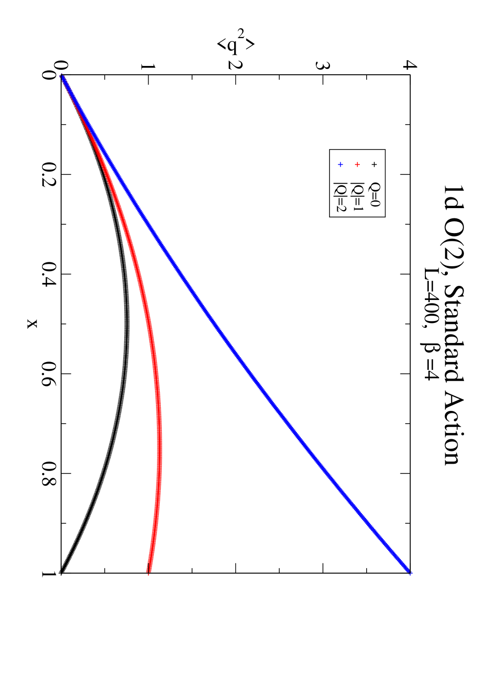
Typical results for and are shown in Fig. 2. In each case they match the expected parabola to high accuracy; this parabola connects with , and with ; the latter is predicted as .


Now we consider the results for the scaling quantity , where is the correlation length. For all three lattice actions the value is known analytically [19, 20] in the thermodynamic limit, . The plots in Fig. 3 illustrate the convergence towards these values (horizontal lines) at fixed , for increasing size. This convergence is manifest, but slow: in particular for the standard action there are permille level finite size effects even at ; these effects are enhanced for increasing .


3.2 Heisenberg model
We proceed to the 2d Heisenberg model, or O(3) model. Here the “scaling term”, , diverges logarithmically in the continuum limit, see e.g. Ref. [20]. Hence we consider just at finite (in lattice units). Again we apply the geometric definition for [21], and we consider the three lattice actions, which are analogous to Subsection 3.1. Fig. 4 shows that the results are very close to the directly measured values of ; those are precise in this case, thanks to the use of the Wolff cluster algorithm, which avoids topological freezing. The data are given in Ref. [15].


We also consider the kurtosis ,
| (3.2) |
which represents a measure of the deviation from a Gaussian distribution (where vanishes). Fig. 5 shows the convergence of the (dimensionless) ratio in the continuum limit towards , the value for a dilute instanton gas; this is best visible for the Manton action.22 2 In the Manton action is classically perfect [19], which explains its excellent scaling behaviour. Apparently its 2d version was used first in Ref. [15], and it has favourable properties as well. Comparing the two plots in Fig. 5 suggests that — in this regime — the volume hardly affects the ratio .33 3 This quantity has been investigated extensively in 4d SU(3) Yang-Mills theory, see e.g. Refs. [22]. According to the latest studies, converges of to a small but finite value around in the continuum and infinite volume limit.


3.3 2-flavour QCD
Finally we proceed to 2-flavour QCD, formulated with the Wilson gauge action. The topological charge density is constructed from the standard lattice field strength tensor. After smoothing, is slightly re-scaled (for optimal proximity to integers [5]) and then rounded to .
For the quarks we used twisted mass fermions (full twist, bare mass ), which leads to a somewhat heavy pion mass, (here we are only interested in testing the slab method). The statistics involved configurations, in (and slab volumes and ) at , which implies a lattice spacing of .
Smoothing was performed by the gradient flow (or Wilson flow in this case), with Runge-Kutta integration in the flow time (step sizes 0.01 and 0.001 yield consistent results). The reference point proposed by Lüscher [23], , requires the flow time .


Fig. 6 (left) shows data for from , after flow time [16]. At extreme values, and (where thin slabs are involved), the data deviate from a parabolic shape. This effect, caused by smoothing, is exponential; at we observed: —deviation— . Therefore we focus on the interval , and perform a joint fit — of all data for — to the shifted parabola
| (3.3) |
which is shown in Fig. 6. This fit works well, and it yields a result for , which perfectly agrees with a direct measurement, and with the result of the AFHO method [12] (cf. Section 1),
| (3.4) |
Regarding the AFHO method, which refers to formula (1.3), the correlations of the topological charge density and the plateau values (after flow time ) are shown in Fig. 6 on the right.
Fig. 7 (left) illustrates the evolution of for flow time , in the sector with (as an example). Longer flow time reduces the statistical errors (the configurations are smoother), but the deviations at the extreme values of are enhanced, and the additive constant in eq. (3.3) becomes more negative.


This constant is required here, but it has not been anticipated in the slab formula (2.1). The plot in Fig. 7 on the right shows that it is consistent with a behaviour , which corresponds to a diffusion process. If we fit the data to the ansatz , we obtain , which confirms that this constant (practically) vanishes at .
4 Conclusions
The slab method is a simple and robust procedure to measure within a fixed topological sector. Hence it is not affected by “topological slowing down”, and it hardly costs any computing time, but there are persistent finite size effects (they tend to be polynomial at fixed topology [9, 10, 11, 12, 13, 15]). It works best at small , which is also the case for the alternative fixed topology methods of Refs. [9, 12]. In contrast to them, however, the only assumption needed for the slab method is a Gaussian distribution of the topological charges, which holds to a very good approximation.44 4 A generalisation which incorporates higher moments in the -distribution is feasible as well.
We reviewed successful tests in O() models [15] and in 2-flavour QCD [16]. In the 2d O(3) model we obtained correct results for to -level, and in the 1d O(2) model far beyond. In 2-flavour QCD, -level precision is attained as well, after gradient flow times . Here an additive constant is required in the fit, and one has to exclude small intervals of close to 0 and 1.
References
- [2] O. Wantz and E.P.S. Shellard, Phys. Rev. D 82 (2010) 123508. C. Bonati et al., JHEP 1603 (2016) 155. P. Petreczky, H.-P. Schadler and S. Sharma, arXiv:1606.03145 [hep-lat]. Sz. Borsanyi et al., arXiv:1606.07494 [hep-lat]. V. Azcoiti, arXiv:1609.01230 [hep-lat].
- [3] W. Bietenholz and S. Shcheredin, Nucl. Phys. B 754 (2006) 17.
- [4] A. Bazavov et al. (MILC Collaboration), Rev. Mod. Phys. 82 (2010) 1349.
- [5] L. Del Debbio, H. Panagopoulos and E. Vicari, JHEP 0208 (2002) 044.
- [6]
S. Schaefer, R. Sommer and F. Virotta
(ALPHA Collaboration),
Nucl. Phys. B 845 (2011) 93.
- [7] M.G. Endres, these proceedings.
- [8] M. Lüscher and S. Schaefer, JHEP 1107 (2011) 036.
- [9] R. Brower, S. Chandrasekharan, J.W. Negele and U.-J. Wiese, Phys. Lett. B 560 (2003) 64.
- [10] A. Dromard and M. Wagner, Phys. Rev. D 90 (2014) 074505.
- [11] W. Bietenholz et al., Phys. Rev. D 93 (2016) 114516.
- [12] S. Aoki, H. Fukaya, S. Hashimoto and T. Onogi, Phys. Rev. D 76 (2007) 054508.
- [13] I. Bautista et al., Phys. Rev. D 92 (2015) 114510.
- [14] P. de Forcrand et al., Nucl. Phys. (Proc. Suppl.) 73 (1999) 578.
- [15] W. Bietenholz, P. de Forcrand and U. Gerber, JHEP 1512 (2015) 070.
- [16] A. Dromard, W. Bietenholz, K. Cichy and M. Wagner, Acta Phys. Polon. Supp. 9 (2016) 635.
- [17] R.C. Brower et al. (LSD Collaboration), Phys. Rev. D 90 (2014) 014503.
- [18] E.V. Shuryak and J.J.M. Verbaarschot, Phys. Rev. D 52 (1995) 295.
- [19] W. Bietenholz, R. Brower, S. Chandrasekharan and U.-J. Wiese, Phys. Lett. B 407 (1997) 283.
- [20] W. Bietenholz, U. Gerber, M. Pepe and U.-J. Wiese, JHEP 12 (2010) 020.
- [21] B. Berg and M. Lüscher, Nucl. Phys. B 190 (1981) 412.
- [22] S. Dürr et al., JHEP 0704 (2007) 055. L. Giusti, S. Petrarca and B. Taglienti, Phys. Rev. D 76 (2007) 094510. H. Panagopoulos and E. Vicari, JHEP 1111 (2011) 119. M. Cè et al., Phys. Rev. D 92 (2015) 074502. C. Bonati, M. D’Elia and A. Scapellato, Phys. Rev. D 93 (2016) 025028.
- [23] M. Lüscher, JHEP 1008 (2010) 071; PoS(LATTICE2010) 015.