Bow shock nebulae of hot massive stars in a magnetized medium

In Fig. 1, we show the gas density field in a series of bow shock models of our initially $20\,\rm M_{\odot}$ star moving with velocity $40\,\rm km\,\rm s^{-1}$ through a medium of ISM background density $n_{\rm H}=0.59\,\rm cm^{-3}$ and of magnetic field strength $B_{\rm ISM}=7\,\mu\rm G$. The crosses indicate the position of the moving star. The figures correspond to a time about $5\,\rm Myr$ after the beginning of the main-sequence phase of the star. The stellar wind and ISM properties are the same for all figures, only the included physics is different for each models (our Table 2). Left-hand panels are hydrodynamical simulations whereas right-hand panels are magneto-hydrodynamical simulations, respectively. From top to bottom, the included thermodynamic processes are adiabatic (a), take into account optically-thin radiative processes of the gas (b), heat transfers (c) or both (d). The black dotted lines are the contours $Q(\mn@boldsymbol{r})=1/2$ which trace the discontinuity between the stellar wind and the ISM gas. The streamlines (a-c) and vector velocity field (d) highlight the penetration of the ISM gas into the different layers of the bow shock.

The internal structure of the bow shocks can be understood by comparing the timescales associated to the different physical processes at work. The dynamical timescale represents the time interval it takes the gas to advect through a given layer of our bow shocks, i.e. the region of shocked ISM or the layer of shocked wind. It is defined as,

where $\Delta l$ is the characteristic lengthscale of the region of the bow shock measured along the $Oz$ direction and where $v$ is the gas velocity in the post-shock region of the considered layers. According to the Rankine-Hugoniot relations and taking into account the non-ideal character of our model, we should have $v\simeq v_{\star}/4$ in the shocked ISM and $v\simeq v_{\rm w}/4$ in the post-region at the forward shock and at the reverse shock, respectively.

The cooling timescale is defined as,

where $\dot{E_{\rm int}}$ is the rate of change of internal energy $E_{\rm int}$ (Orlando et al., 2005). The heat conduction timescale measures the rapidity of heat transfer into the bow shock, and is given by,

where $l$ is a characteristic length of the bow shock along which heat transfers take place. Measuring the density, pressure and velocity fields in our simulations, we evaluate and compare those quantities defined in Eqs. (18)-(20) at both the post-shock regions at the forward and reverse shocks. Results for both the layers of shocked wind and shocked ISM material are given in Table 3.

Our hydrodynamical, dissipation-free bow shock model HD2040Ideal has a morphology governed by the gas dynamics only (Fig. 1a). It has a contact discontinuity separating the outer region of cold shocked ISM from the inner region of hot shocked stellar wind, which are themselves bordered by the forward and reverse shocks, respectively. There is no advection of ISM material into the wind region (see the ISM gas streamlines in Fig. 1a). The model HD2040Cool including cooling by optically-thin radiation has a considerably reduced layer of dense, shocked ISM gas caused by the rapid losses of internal energy ($t_{\rm dyn}\gg t_{\rm cool}$, see timescales in our Table 3). Its thinness favours the growth of Kelvin-Helmholtz instabilities and allows large eddies to develop in the shocked regions (Fig. 1b). The layer of hot gas is isothermal because the regular wind momentum input at the reverse shock prevents it from cooling and it therefore conserves its hot temperature ($t_{\rm cool}\gg t_{\rm dyn}$) whereas the distance between the star and the contact discontinuity,

does not evolve (Wilkin, 1996).

The model HD2040Heat takes into account thermal conduction which is isotropic in the case of the absence of magnetic field. The heat flux reads,

and transports internal energy from the reverse shock to the contact discontinuity ($t_{\rm dyn}\gg t_{\rm heat}$) which in its turn splits the dense region into a hot ($t_{\rm dyn}\gg t_{\rm heat}$) and a cold layer of shocked ISM gas ($t_{\rm dyn}\ll t_{\rm heat}$), respectively. This modifies the penetration of ISM gas into the bow shock and causes the region of shocked wind to shrink to a narrow layer of material close to the reverse shock (Fig. 1c). Not surprisingly, the model with both cooling and conduction HD2040All (Fig. 1d) presents both the thermally split region of shocked ISM ($t_{\rm dyn}\ll t_{\rm heat}$, $t_{\rm dyn}\gg t_{\rm cool}$, $t_{\rm cool}\ll t_{\rm heat}$) and a reduced layer of shocked wind material ($t_{\rm dyn}\gg t_{\rm heat}$, $t_{\rm dyn}\ll t_{\rm cool}$, $t_{\rm cool}\gg t_{\rm heat}$) that reorganises the internal structure of the bow shock together with a dense shell of cool ISM gas (see the also discussion in Paper I). For the sake of clarity Fig. 1d overplots the gas velocity fields as white arrows which illustrate the penetration of ISM gas into the hot layer of the bow shock.

We plot in the right-hand panels of Fig. 1 the ideal magneto-hydrodynamical simulation of our initially $20\,\rm M_{\odot}$ star moving with $v_{\star}=40\,\rm km\,\rm s^{-1}$ through a medium where the strength of the magnetic field is $B_{\rm ISM}=7\,\mu\rm G$ (e) together with models including cooling and heating by optically-thin radiation (f), anisotropic heat conduction (g) and both (h). Despite of the fact that the overall morphology of our magneto-hydrodynamical bow shock models is globally similar to the models with $B_{\rm ISM}=0\,\mu\rm G$, a given number of significant changes relative to both their shape and internal structure arise. Note that in the context of our magneto-hydrodynamical models, $t_{\rm heat}$ represents the heat transfer timescale normal to the fields lines.

Our ideal magneto-hydrodynamical model has the typical structure of a stellar wind bow shock, with a region of shocked ISM gas surrounding the one of shocked wind gas. The contact discontinuity acts as a border between the two kind of material (Fig. 1e). The model with cooling MHD2040CoolB7 has reduced but denser layer of ISM gas (Fig. 1f) due to the rapid cooling time ($t_{\rm cool}\ll t_{\rm dyn}$). The magneto-hydrodynamical model with thermal conduction is similar to our model MHD2040IdealB7 since, due to his anisotropic character, heat transport are canceled across the magnetic field lines ($t_{\rm heat}\ggg t_{\rm dyn}$). Note the boundary effect close to the apex along the $Oz$ direction as a result of the heat conduction along the direction of the ISM magnetic field lines (Fig. 1g). Finally, our model with both processes has its dynamics governed by the cooling in the region of shocked ISM ($t_{\rm heat}\ggg t_{\rm dyn}$, $t_{\rm heat}\ggg t_{\rm cool}$, $t_{\rm cool}\ll t_{\rm dyn}$) and by the wind momentum in the region of shocked wind ($t_{\rm heat}\ggg t_{\rm dyn}$, $t_{\rm heat}\ggg t_{\rm cool}$, $t_{\rm dyn}\ll t_{\rm cool}$).

The shape of the bow shock generated around a runaway massive star in the warm phase of the ISM is a function of the respective strength of both the ISM ram pressure $\rho_{\rm ISM}v_{\star}^{2}$ and the stellar wind ram pressure $\rho_{\rm w}v_{\rm w}^{2}$, as seen in the frame of reference of the moving object (Mohamed et al., 2012, see explanations in). According to Eq. (15), $\rho_{w}=\dot{M}/4\pi r^{2}v_{\rm w}$ which implies that $\rho_{\rm w}v_{\rm w}^{2}\propto\dot{M}v_{\rm w}$. In other words, in a given ambient medium and at a given peculiar velocity, the governing quantity in the shaping of such bow shock is $\dot{M}\rm v_{w}$ and its stand-off distance $R(0)$ goes as $\sqrt{\dot{M}v_{w}}$, see Eq. (21). Nevertheless, if the production of stellar evolution models depends on specific prescriptions relative to $\dot{M}$ that are consistently used through the calculations (Kudritzki et al., 1989, in our case the recipe of), the estimate of the wind velocity is posterior to the calculation of the stellar structure and it does not influence $\dot{M}$, $T_{\rm eff}$ or $L_{\star}$.

The manner to calculate $\rm v_{w}$ is not unique (Castor et al., 1975; Kudritzki et al., 1989; Kudritzki & Puls, 2000; Eldridge et al., 2006) and it can also be assumed to characteristic values for the concerned stars (Comerón & Kaper, 1998; van Marle et al., 2014; van Marle et al., 2015; Acreman et al., 2016). In our study, the wind velocities are in the lower limit of the range of validity for the main-sequence massive stars that we consider, nonetheless, they still remain within the order of magnitude of, e.g. late O stars (Martins et al., 2007) or weak-winded stars (Comerón & Kaper, 1998). Furthermore, the evolution of massive stars are governed by physical mechanisms strongly influencing their feedback such as the presence of low-mass companions (Sana et al., 2012), which are neglected in our stellar evolution models. Produced before their zero-age main-sequence phase, e.g. by fragmentation of the accretion disk that surrounds massive protostars (Meyer et al., 2016), those dwarf stars entirely modify the evolution of massive stars and consequently affect their wind properties (de Mink et al., 2007; de Mink et al., 2009; Paxton et al., 2011; Marchant et al., 2016).

Using wind velocities faster by a factor $\alpha$ would enlarge the bow shocks by a factor $\sqrt{\alpha}$ and, eventually, in the hydrodynamical case, favorise the growth of instabilities (cf. Fig. 1b). However, the results of our numerical study would be similar in the sense that the presence of the field essentially stabilises the nebulae and inhibits the effects of heat conduction (cf. Fig. 1a,h), reduces their size (Section 3.2.1) and modifies, e.g. their infrared emission accordingly (see Section 4.3). In Fig. 2, we compare our values of $\dot{M}v_{w}$ (Table 1) with the non-rotating stellar evolutionary models published in Brott et al. (2011). We conclude that the bow shocks generated with our initially $10$, $20$ and $40\,\rm M_{\odot}$ weak-winded stellar models correspond to nebulae produced by initially $\approx 10$, $\approx 18$ and $\approx 32\,\rm M_{\odot}$ standard massive stars at Galactic metallicity, respectively. Therefore, our models have full validity for this study of magnetized bow shock nebulae, albeit of lower zero-age main-sequence mass in the case of our heaviest runaway star.

The ISM magnetic pressure, proportional to $\vec{B}_{\rm ISM}^{2}$, dynamically compresses the region of shocked ISM gas such that the density in the post-shock region at the forward shock slightly increases. Similarly, the shape of the bow shock’s wings of shocked ISM are displaced sidewards compare to our model with $B_{\rm ISM}=0\,\mu\rm G$ (Fig. 1a,e). The size of the layer of ISM gas diminishes along the direction of motion of the moving star and the position of the termination shock sets at a distance from the star where the wind ram pressure equals the ISM total pressure decreases as measured along the $Oz$ axis. The effects of the cooling is standard in the sense that it makes the region of shocked ISM thinner and denser, i.e. the position of the forward shock decreases, together with the bow shock volume. The effects of heat conduction are canceled ($t_{\rm dyn}\ll t_{\rm heat}$) in the direction perpendicular to the field lines, i.e. in the direction perpendicular to the streamline collinear to both the reverse shock and the contact discontinuity.

The topology at the apex of our magneto-hydrodynamical bow shock (Fig. 1h) is different from the traditional single-front bow shock morphology (Fig. 1d). This can be discussed at the light of plasma physics studies (de Sterck et al., 1998; de Sterck & Poedts, 1999). These works explore the formation of exotic shocks and discontinuities that affect the particularly dimpled apex of bow shocks generated by field-aligned flows around a conducting cylinder (de Sterck et al., 1998). They extended this result to bow shocks produced around a conducting sphere and showed that the inflow parameter space leading to such structures is similar to plasma $\beta$ and Alfvénic Mach number values allowing the formation of so-called switch-on shocks (de Sterck & Poedts, 1999).

Switch-on shocks are allowed when plasma $\beta$ of the inflowing material, i.e. the ratio of the gas and magnetic pressures, which read,

and its Alfvénic Mach number,

where,

is the Alfvénic velocity, satisfy some particular conditions. Note that in Eq. (24) the velocities are taken along the shock normal. On the one hand, the plasma beta must be such that,

whereas on the other hand, the Alfvénic Mach number verifies the following order relation,

where $\gamma$ is the adiabatic index, see Eq. 1 in Pogorelov & Matsuda (2000). Numbers from our simulations indicate that the ISM thermal pressure $n_{\rm ISM}k_{\rm B}T_{\rm ISM}\approx 8.62\times 10^{-13}\,\rm dyne\,\rm s^{-2}$, therefore we find $\beta>2/\gamma\approx 1.2$ for $B_{\rm ISM}\leq 3.5\,\mu\rm G$ (see bow shocks with normal morphologies in Fig. 3a,b) but $\beta\approx{\color[rgb]{0,0,0}0.44}<2/\gamma\approx 1.2$ for $B_{\rm ISM}=7\,\mu\rm G$ (see dimpled bow shock in Fig. 3c). The Alfvénic Mach number $M_{\rm A}=v/v_{\rm A}\approx 40.0\,\rm km\,\rm s^{-1}/17.2\,\rm km\,\rm s^{-1}\approx 2.33$ which is outside the range $1<M_{\rm A}<((\gamma(1-\beta)+1)/(\gamma-1))^{1/2}\approx{\color[rgb]{0,0,0}1.70}$. Similarly, the model with $v_{\star}=70\,\rm km\,\rm s^{-1}$ is such that $M_{\rm A}>((\gamma(1-\beta)+1)/(\gamma-1))^{1/2}$ whereas our slower model with $v_{\star}=20\,\rm km\,\rm s^{-1}$ gives $1<M_{\rm A}\approx 1.16<((\gamma(1-\beta)+1)/(\gamma-1))^{1/2}$, which is inside the range in Eq. (27). We conclude that the upstream ISM conditions in our magneto-hydrodynamical simulations producing dimpled bow shocks have values consistent with the existence of switch-on shocks, see also sketch of the ($\beta$,$M_{\rm A}$) plane in Fig. 3 of de Sterck & Poedts (1999).

However, we can not affirm that the dimpled apex topology of our magneto-hydrodynamical bow shocks models is of origin similar to the ones in de Sterck et al. (1998); de Sterck & Poedts (1999). Only their particular concave-inward form that differs from the classical shape of hydrodynamical bow shocks (Fig. 1e) authorizes a comparison between the two studies. Nevertheless, we notice that our bow shocks are also generated in an ambient medium in which the plasma beta and the Alfvénic Mach number have parameter values consistent with the formation of switch-on shocks, which has been showed to be similar to the parameter values producing dimpled bow shocks around charged obstacles (see de Sterck et al., 1998; de Sterck & Poedts, 1999, and references therein). Additional investigations, left for future studies, are required to assess the question of the exact nature the various discontinuities affecting magneto-hydrodynamical bow shocks of OB stars.

Fig. 3 is similar to Fig. 1 and displays the effects of the ISM magnetic field strength $B_{\rm ISM}=0$ (a), $3.5$ (b) and $7.0\,\rm\mu G$ (c) on the shape of the bow shocks produced by our initially $20\,\rm M_{\odot}$ star moving with velocity $v_{\star}=40\,\rm km\,\rm s^{-1}$. In Fig. 12 we show density (solid lines) and temperature (dotted lines) profiles from our hydrodynamical simulation (thick blue lines) and magneto-hydrodynamical model (thin red lines) of the bow shocks in Fig. 3. The profiles are taken along the symmetry axis of the computational domain. The global structure of the bow shock is similar for both simulations, i.e. it consists of a hot bubble ($T\approx\,10^{7}\,\rm K$) surrounded by a shell of dense ($n\approx\,10\,\rm cm^{-3}$) shocked ISM gas. The profiles in Fig. 12 highlights the progressive compression of the bow shocks by the the ISM total pressure which magnetic component increases as $B_{\rm ISM}$ is larger. Several mechanisms at work might be responsible for such discrepancy:

1. 1.

   The magnetic pressure in the ISM. If one neglects the thermal pressures $nk_{\rm B}T$ in both the supersonic stellar wind and the inflowing ISM, and omits the magnetic pressure $\propto B_{\star}^{2}\propto r^{-4}$ at the wind termination shock, then the pressure balance between ISM and stellar wind gas reads,

   $$\rho_{\rm w}v_{\mathrm{w}}^{2}=\rho_{\rm ISM}v_{\star}^{2}+\frac{B_{\rm ISM}^{2}}{8\pi},$$

   (28)

   from which one can derive the bow shock stand-off distance in a planar-aligned field bow shock,

   $$R(0)=\Bigg(\frac{2\dot{M}v_{\mathrm{w}}}{B_{\rm ISM}^{2}+8\pi\rho_{\mathrm{ISM}}v_{\star}^{2}}\Bigg)^{1/2},$$

   (29)

   that is slightly smaller from the one derived in a purely hydrodynamical context (Wilkin, 1996).

2. 2.

   The cooling by optically-thin radiative processes. Changes in the density at the post-shock region at the forward shock influence the temperature in the shocked ISM gas, which in their turn modify the cooling rate of the gas, itself affecting its thermal pressure. This results in an increase of the density of the shell of ISM gas but also a decrease of the temperature in the hot region of shocked stellar wind material that shrinks in order to maintain its total pressure equal to $\rho_{\rm ISM}v_{\star}^{2}+B_{\rm ISM}^{2}/8\pi$.

3. 3.

   The magnetic field field lines inside the bow shock. The compression of the layer of shocked ISM gas modifies the arrangement of the field lines in the post-shock region at the forward shock. Thus, the term $B_{\rm ISM}^{2}/8\pi$ corresponding to the magnetic pressure increases and modifies the effects of radiative cooling in the simulations (see above).

4. 4.

   Symmetry effects. The solution may also be affected by the intrinsic two-dimensional nature of our simulations, which may develop numerical artifices close to the symmetry axis. In the case of magneto-hydrodynamical simulations of objects moving supersonically along the direction of the ISM magnetic field, such effects are more complex than a simple accumulation of material at the apex of the nebula, but might present artificial shocks, see also Section 3.4.

Appreciating in detail which of the above cited processes dominates the solution would require three-dimensional numerical simulations which are beyond the scope of this work. Moreover, establishing an analytic theory of the position of the contact discontinuity of a magnetized bow shock is a non-trivial task since the thin-shell limit (Wilkin, 1996) is not applicable. In particular, the hot bubble loses about three quarter of its size along the $Oz$ direction when the ISM magnetic field strength increases up to $B_{\rm ISM}=7\,\mu\rm G$ (Fig. 3a,c). This modifies the volume of hot shocked ISM gas advected thanks to heat transfers towards the inner part of the bow shock of our model HD2040All, reducing it to a narrow layer made of shocked wind material since anisotropic thermal conduction forbids the penetration of ISM gas in the hot region. The effects of the ISM magnetisation on our optical and infrared bow shocks’ emission properties are further discussed in Section 4.

All of our magneto-hydrodynamical simulations have a stable density field (Fig. 1e,f,g,h). The simulations with cooling but without heat transfer (Fig. 1b) show that the presence of the magnetic field inhibits the growth of Kelvin-Helmholtz instabilities (Fig. 1f) that typically develops within the contact discontinuity of the bow shocks because they are the interface of two plasma moving in opposite directions (Comerón & Kaper, 1998; van Marle et al., 2007, Paper I). The solution does not change performing the simulation MHD2040AllB7 at double and quadruple spatial resolution, and conclude that our results are consistent with both numerical studies devoted to the growth and saturation of these instabilities in the presence of a planar magnetic field (Keppens et al., 1999, see, e.g.) and with results obtained for slow-winded, cool runaway stars moving in a planar-aligned magnetic field (van Marle et al., 2014). Note that detailed numerical studies demonstrating the suppression of shear instabilities by the presence of a background magnetic field also exist in the context of jets from protostars (Viallet & Baty, 2007).

Fig. 9b plots a comparison betwenn the SEDs of two bow shock models generated by our $20\,\rm M_{\odot}$ star moving with velocity $40\,\rm km\,\rm s^{-1}$, either through an unmagnetized ISM (model MS2040, solid blue line) or in a medium with $B_{\rm ISM}=7\,\mu\rm G$ (model MHD2040AllB7, dotted red line) for a viewing angle of the nebulae of $\phi=0^{\circ}$. The figure represents the flux density $F_{\lambda}$ (in $\rm Jy$) as a function of the wavelength $\lambda$ (in $\mu\rm m$) for the waveband including the $0.01\leq\lambda\leq 2000\,\mu\rm m$. The star is responsible for the component in the range $0.01\leq\lambda\leq 10\,\mu\rm m$ that corresponds to a black body spectrum of temperature $T_{\rm eff}=33900\,\rm K$ (see Table 1) while the circumstellar dust produces the feature in the waveband $10\leq\lambda\leq 2000\,\mu\rm m$. The bow shock’s component is in the waveband including the wavelengths at which stellar wind bow shock are typically recorded, e.g. at $60\,\mu\rm m$ van Buren & McCray (1988a); van Buren et al. (1995); Noriega-Crespo et al. (1997).

The SED of the magnetized bow shock has a slightly larger flux than the SED of the hydrodynamical bow shock in the waveband $10\leq\lambda\leq 30\,\mu\rm m$, because its smaller size makes the shell of dense ISM gas closer to the star, increasing therefore the dust temperature (Fig. 9b). At $\lambda\approx 30\,\mu\rm m$, the hydrodynamical bow shock emits by slightly more than half an order of magnitude than the magnetized nebula, e.g. at $\lambda\approx 60\,\mu\rm m$ our model MS2040 has a density flux $F_{\lambda}\approx 3\times 10^{-1}\,\rm Jy$ whereas our model MHD2040AllB7 shows $F_{\lambda}\approx 1\times 10^{-1}\,\rm Jy$, respectively. This is consistent with the previously discussed reduction of the projected optical emission of our bow shocks. This relates to the changes in size of the nebulae induced by the inclusion of the magnetic field in our simulations, which reduces the mass of dust in the structure responsible for the reprocessing of the starlight, e.g. our models MS2040 and MHD2040AllB7 contain about $M_{\rm d}\approx 3\times 10^{-2}\,\rm M_{\odot}$ and $M_{\rm d}\approx 2\times 10^{-3}\,\rm M_{\odot}$, respectively, where $M_{\rm d}$ is the dust mass trapped into the nebulae. The reduced mass of dust into the magnetized bow shock absorbs a lesser amount of the stellar radiation and therefore re-emits a smaller quantity of energy, reducing $F_{\lambda}$ in the waveband $\lambda\geq\,30\,\mu$m (Fig. 9b). Note that the infrared surface brightness of a bow shock is also sensible to the density of its ambient medium, i.e. $F_{\lambda}$ is much larger in the situation of a runaway star moving in a medium with $n_{\rm ISM}\simeq 1000\,\rm cm^{-3}$ (Acreman et al., 2016).

Our Fig. 10 plots a series of synthetic infrared emission maps of our bow shock models produced by an initially $20\,\rm M_{\odot}$ star moving with velocity $40\,\rm km\,\rm s^{-1}$ in its purely hydrodynamical (MS2040) or magneto-hydrodynamical configuration (MHD2040AllB7) at the wavelengths corresponding to the central wavelengths of the IRAS facility’s main broadband images (van Buren & McCray, 1988b), i.e. $\lambda=25\,\rm\mu m$ (left column of panels), $60\,\rm\mu m$ (middle column of panels) and $100\,\rm\mu m$ (right column of panels). The maps are represented with an inclination angle of $\phi=30^{\circ}$ (Fig. 10a,e,i), $45^{\circ}$ (Fig. 10b,f,j), $60^{\circ}$ (Fig. 10c,g,k) and $90^{\circ}$ (Fig. 10d,h,l) with respect to the plane of the sky and the projected flux is plotted in units of $\rm erg\,\rm s^{-1}\,\rm cm^{-2}\,\rm arcsec^{-2}$. As in the context of their optical emission (Fig. 7), the overall size of the infrared magnetized bow shocks is smaller than in the hydrodynamical case because of the reduction of their stand-off distance $R(0)$, see, e.g. Fig. 10a,e,j. The global morphology of our infrared bow shock nebulae does not change significantly. It remains a single, bright arc at the front of an ovoid structure that is symmetric with respect to the direction of motion of the runaway star and extended to the trail ($z\leq 0$) of the bow shocks due to the supersonic motion of the star Acreman et al. (2016). In the hydrodynamical case, the region of maximum emission is the region containing the ISM dust which temperature is smaller than a few $10^{4}\,\rm K$, i.e. between the contact discontinuity and the forward shock of the bow shock (Acreman et al., 2016, Paper I,) whereas in the magnetized case, the maximum emission is reduced to a thin region close to the discontinuity between hot stellar wind and colder ISM. Both the shocked stellar wind and the shocked ISM of the bow shock do not contributes to these emission because the material is too hot.

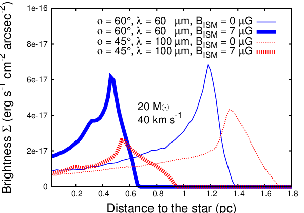
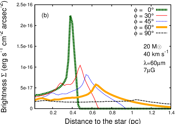
Fig. 11 reports cross-sections taken along the direction of motion of the bow shock and comparing their surface brightesses at several wavebands $\lambda$ and viewing angles $\phi$. It illustrates that, as in the case of the optical emission, the presence of the ISM magnetic field makes the bow shocks slightly dimmer, e.g. for $\phi=45^{\circ}$ our model has a maximal surface brighness of $\Sigma^{\rm max}_{100\,\mu\rm m}\approx 4.3\times 10^{-17}\,\rm erg\,\rm s^{-1}\,\rm cm^{-2}\,\rm arcsec^{-2}$ whereas $\Sigma^{\rm max}_{100\,\mu\rm m}\approx 2.6\times 10^{-17}\,\rm erg\,\rm s^{-1}\,\rm cm^{-2}\,\rm arcsec^{-2}$ for $B_{\rm ISM}=0$ and $7\,\mu\rm G$, respectively. Fig. 12 shows different cross-sections of the projected infrared emission the magnetized bow shock of our initially $20\,\rm M_{\odot}$ star moving with velocity $v_{\star}=40\,\rm km\,\rm s^{-1}$. The emission at $\lambda=60\,\mu\rm m$ is more important that at $\lambda=25\,\mu\rm m$ and at $\lambda=100\,\mu\rm m$, e.g. it peaks at $\Sigma^{\rm max}_{60\,\mu\rm m}\approx 8.2\times 10^{-17}\,\rm erg\,\rm s^{-1}\,\rm cm^{-2}\,\rm arcsec^{-2}$ whereas $\Sigma^{\rm max}_{25\,\mu\rm m}\approx 2.6\times 10^{-17}\,\rm erg\,\rm s^{-1}\,\rm cm^{-2}\,\rm arcsec^{-2}$ and $\Sigma^{\rm max}_{100\,\mu\rm m}\approx 3.0\times 10^{-17}\,\rm erg\,\rm s^{-1}\,\rm cm^{-2}\,\rm arcsec^{-2}$, respectively, at a distance of $0.55\,\rm pc$ from the star and assuming an inclination angle of the bow shock of $\phi=45^{\circ}$ (Fig. 12a). All our models have similar behaviour of their infrared surface brightness as a function of $\lambda$ and $\phi$. Note also that the evolution of the position of the stand-off distance of the bow shock is consistent with the study of Acreman et al. (2016) in the sense that it increases at larger $\phi$ (Fig. 12b).

References

- Acreman et al. (2016) Acreman D. M., Stevens I. R., Harries T. J., 2016, MNRAS, 456, 136
- Alexiades et al. (1996) Alexiades V., Amiez G., Gremaud P.-A., 1996, Communication in Numerical Methods in Engineering, 12, 31
- Arnaud (1996) Arnaud K. A., 1996, in Jacoby G. H., Barnes J., eds, Astronomical Data Analysis Software and Systems V Vol. 101 of Astronomical Society of the Pacific Conference Series, XSPEC: The First Ten Years. p. 17
- Arthur & Hoare (2006) Arthur S. J., Hoare M. G., 2006, ApJS, 165, 283
- Asplund et al. (2009) Asplund M., Grevesse N., Sauval A. J., Scott P., 2009, ARA&A, 47, 481
- Balsara et al. (2008) Balsara D. S., Tilley D. A., Howk J. C., 2008, MNRAS, 386, 627
- Baranov et al. (1996) Baranov V. B., Barmin A. A., Pushkar’ E. A., 1996, Astronomy Letters, 22, 555
- Baranov et al. (1975) Baranov V. B., Krasnobaev K. V., Onishchenko O. G., 1975, Soviet Astronomy Letters, 1, 81
- Baranov & Malama (1993) Baranov V. B., Malama Y. G., 1993, J. Geophys. Res., 98, 15157
- Bjorkman & Wood (2001) Bjorkman J. E., Wood K., 2001, ApJ, 554, 615
- Blondin & Koerwer (1998) Blondin J. M., Koerwer J. F., 1998, New Ast., 3, 571
- Bohren & Huffman (1983) Bohren C. F., Huffman D. R., 1983, Absorption and scattering of light by small particles
- Boley et al. (2013) Boley A. C., Morris M. A., Desch S. J., 2013, ApJ, 776, 101
- Brighenti & D’Ercole (1994) Brighenti F., D’Ercole A., 1994, MNRAS, 270, 65
- Brighenti & D’Ercole (1995a) Brighenti F., D’Ercole A., 1995a, MNRAS, 277, 53
- Brighenti & D’Ercole (1995b) Brighenti F., D’Ercole A., 1995b, MNRAS, 273, 443
- Brott et al. (2011) Brott I., de Mink S. E., Cantiello M., Langer N., de Koter A., Evans C. J., Hunter I., Trundle C., Vink J. S., 2011, A&A, 530, A115
- Brown & Bomans (2005) Brown D., Bomans D. J., 2005, A&A, 439, 183
- Burlaga et al. (2015) Burlaga L. F., Florinski V., Ness N. F., 2015, ApJ, 804, L31
- Castor et al. (1975) Castor J. I., Abbott D. C., Klein R. I., 1975, ApJ, 195, 157
- Chalov et al. (2016) Chalov S. V., Malama Y. G., Alexashov D. B., Izmodenov V. V., 2016, MNRAS, 455, 431
- Chiotellis et al. (2016) Chiotellis A., Boumis P., Nanouris N., Meaburn J., Dimitriadis G., 2016, MNRAS, 457, 9
- Chiotellis et al. (2012) Chiotellis A., Schure K. M., Vink J., 2012, A&A, 537, A139
- Chita et al. (2008) Chita S. M., Langer N., van Marle A. J., García-Segura G., Heger A., 2008, A&A, 488, L37
- Churchwell et al. (2006) Churchwell E., Povich M. S., Allen D., Taylor M. G., Meade M. R., Babler B. L., Indebetouw R., Watson C., Whitney B. A., Wolfire M. G., Bania T. M., Benjamin R. A., Clemens 2006, ApJ, 649, 759
- Comerón & Kaper (1998) Comerón F., Kaper L., 1998, A&A, 338, 273
- Cowie & McKee (1977) Cowie L. L., McKee C. F., 1977, ApJ, 211, 135
- Cox et al. (1991) Cox C. I., Gull S. F., Green D. A., 1991, MNRAS, 250, 750
- Cox et al. (2012) Cox N. L. J., Kerschbaum F., van Marle A. J., Decin L., Ladjal D., Mayer A., 2012, A&A, 543, C1
- Crutcher et al. (1999) Crutcher R. M., Roberts D. A., Troland T. H., Goss W. M., 1999, ApJ, 515, 275
- de Jager et al. (1988) de Jager C., Nieuwenhuijzen H., van der Hucht K. A., 1988, A&AS, 72, 259
- de Mink et al. (2009) de Mink S. E., Cantiello M., Langer N., Pols O. R., Brott I., Yoon S.-C., 2009, A&A, 497, 243
- de Mink et al. (2007) de Mink S. E., Pols O. R., Hilditch R. W., 2007, A&A, 467, 1181
- de Sterck et al. (1998) de Sterck H., Low B. C., Poedts S., 1998, Physics of Plasmas, 5, 4015
- de Sterck & Poedts (1999) de Sterck H., Poedts S., 1999, A&A, 343, 641
- de Sterck & Poedts (2000) de Sterck H., Poedts S., 2000, in Verheest F., Goossens M., Hellberg M. A., Bharuthram R., eds, Waves in Dusty, Solar, and Space Plasmas Vol. 537 of American Institute of Physics Conference Series, Disintegration and reformation of intermediate shock segments in 3D MHD bow shock flows. pp 232–239
- de Sterck & Poedts (2001) de Sterck H., Poedts S., 2001, in Freistühler H., Warnecke G. m. . f. p. . ., eds, Waves in Dusty, Solar, and Space Plasmas Vol. 141 of International Series of Numerical Mathematics, Overcompressive shocks and compound shocks in 2D and 3D magnetohydrodynamic flows
- del Valle et al. (2015) del Valle M. V., Romero G. E., Santos-Lima R., 2015, MNRAS, 448, 207
- Diaz-Miller et al. (1998) Diaz-Miller R. I., Franco J., Shore S. N., 1998, ApJ, 501, 192
- Donati et al. (2002) Donati J.-F., Babel J., Harries T. J., Howarth I. D., Petit P., Semel M., 2002, MNRAS, 333, 55
- Dopita (1973) Dopita M. A., 1973, A&A, 29, 387
- Draine (2011) Draine B. T., 2011, Physics of the Interstellar and Intergalactic Medium
- Draine & Lee (1984) Draine B. T., Lee H. M., 1984, ApJ, 285, 89
- Dullemond (2012) Dullemond C. P., , 2012, RADMC-3D: A multi-purpose radiative transfer tool, Astrophysics Source Code Library
- Dyson (1975) Dyson J. E., 1975, Ap&SS, 35, 299
- Eldridge et al. (2006) Eldridge J. J., Genet F., Daigne F., Mochkovitch R., 2006, MNRAS, 367, 186
- Eldridge et al. (2011) Eldridge J. J., Langer N., Tout C. A., 2011, MNRAS, 414, 3501
- Esquivel et al. (2010) Esquivel A., Raga A. C., Cantó J., Rodríguez-González A., López-Cámara D., Velázquez P. F., De Colle F., 2010, ApJ, 725, 1466
- Evans & Massey (2015) Evans K. A., Massey P., 2015, AJ, 150, 149
- Fiedler & Mouschovias (1993) Fiedler R. A., Mouschovias T. C., 1993, ApJ, 415, 680
- Fitzenreiter et al. (1990) Fitzenreiter R. J., Scudder J. D., Klimas A. J., 1990, J. Geophys. Res., 95, 4155
- Florinski et al. (2004) Florinski V., Pogorelov N. V., Zank G. P., Wood B. E., Cox D. P., 2004, ApJ, 604, 700
- Gaensler (1998) Gaensler B. M., 1998, ApJ, 493, 781
- Golub & Pasachoff (1997) Golub L., Pasachoff J. M., 1997, The Solar Corona, Cambridge University Press
- Gull & Sofia (1979) Gull T. R., Sofia S., 1979, ApJ, 230, 782
- Gvaramadze et al. (2012) Gvaramadze V. V., Langer N., Mackey J., 2012, MNRAS, 427, L50
- Gvaramadze et al. (2014) Gvaramadze V. V., Menten K. M., Kniazev A. Y., Langer N., Mackey J., Kraus A., Meyer D. M.-A., Kamiński T., 2014, MNRAS, 437, 843
- Harten et al. (1983) Harten A., Lax P. D., van Leer B., 1983, SIAM Review, 25, 35
- Harvey-Smith et al. (2011) Harvey-Smith L., Madsen G. J., Gaensler B. M., 2011, ApJ, 736, 83
- Heger et al. (2005) Heger A., Woosley S. E., Spruit H. C., 2005, ApJ, 626, 350
- Heiligman (1980) Heiligman G. M., 1980, MNRAS, 191, 761
- Heitsch et al. (2007) Heitsch F., Slyz A. D., Devriendt J. E. G., Hartmann L. W., Burkert A., 2007, ApJ, 665, 445
- Huthoff & Kaper (2002) Huthoff F., Kaper L., 2002, A&A, 383, 999
- Kaper et al. (1997) Kaper L., van Loon J. T., Augusteijn T., Goudfrooij P., Patat F., Waters L. B. F. M., Zijlstra A. A., 1997, ApJ, 475, L37
- Kawamura et al. (2010) Kawamura A. D., Heerikhuisen J., Pogorelov N. V., 2010, AGU Fall Meeting Abstracts
- Keppens et al. (1999) Keppens R., Tóth G., Westermann R. H. J., Goedbloed J. P., 1999, Journal of Plasma Physics, 61, 1
- Kobulnicky et al. (2016) Kobulnicky H. A., Chick W. T., Schurhammer D. P., Andrews J. E., Povich M. S., Munari S. A., Olivier G. M., Sorber R. L., Wernke H. N., Dale D. A., Dixon D. M., 2016, ArXiv e-prints:1609.02204
- Kroupa (2001) Kroupa P., 2001, MNRAS, 322, 231
- Kudritzki et al. (1989) Kudritzki R. P., Pauldrach A., Puls J., Abbott D. C., 1989, A&A, 219, 205
- Kudritzki & Puls (2000) Kudritzki R.-P., Puls J., 2000, ARA&A, 38, 613
- Langer (2012) Langer N., 2012, ARA&A, 50, 107
- Langer et al. (1999) Langer N., García-Segura G., Mac Low M.-M., 1999, ApJ, 520, L49
- Linde et al. (1998) Linde T. J., Gombosi T. I., Roe P. L., Powell K. G., Dezeeuw D. L., 1998, J. Geophys. Res., 103, 1889
- Lodders (2003) Lodders K., 2003, ApJ, 591, 1220
- Lopez et al. (2011) Lopez R. E., Merkin V. G., Lyon J. G., 2011, Annales Geophysicae, 29, 1129
- Lucy (1999) Lucy L. B., 1999, A&A, 344, 282
- Mac Low et al. (1991) Mac Low M.-M., van Buren D., Wood D. O. S., Churchwell E., 1991, ApJ, 369, 395
- Mackey et al. (2016) Mackey J., Haworth T. J., Gvaramadze V. V., Mohamed S., Langer N., Harries T. J., 2016, A&A, 586, A114
- Mackey et al. (2013) Mackey J., Langer N., Gvaramadze V. V., 2013, MNRAS
- Mackey et al. (2014) Mackey J., Mohamed S., Gvaramadze V. V., Kotak R., Langer N., Meyer D. M.-A., Moriya T. J., Neilson H. R., 2014, Nature, 512, 282
- Mackey et al. (2012) Mackey J., Mohamed S., Neilson H. R., Langer N., Meyer D. M.-A., 2012, ApJ, 751, L10
- Marchant et al. (2016) Marchant P., Langer N., Podsiadlowski P., Tauris T. M., Moriya T. J., 2016, A&A, 588, A50
- Martins et al. (2007) Martins F., Genzel R., Hillier D. J., Eisenhauer F., Paumard T., Gillessen S., Ott T., Trippe S., 2007, A&A, 468, 233
- Mathis et al. (1977) Mathis J. S., Rumpl W., Nordsieck K. H., 1977, ApJ, 217, 425
- McComas et al. (2015) McComas D. J., Bzowski M., Frisch P., Fuselier S. A., Kubiak M. A., Kucharek H., Leonard T., Möbius E., Schwadron N. A., Sokół J. M., Swaczyna P., Witte M., 2015, ApJ, 801, 28
- Meyer et al. (2014) Meyer D. M.-A., Gvaramadze V. V., Langer N., Mackey J., Boumis P., Mohamed S., 2014, MNRAS, 439, L41
- Meyer et al. (2015) Meyer D. M.-A., Langer N., Mackey J., Velázquez P. F., Gusdorf A., 2015, MNRAS, 450, 3080
- Meyer et al. (2014) Meyer D. M.-A., Mackey J., Langer N., Gvaramadze V. V., Mignone A., Izzard R. G., Kaper L., 2014, MNRAS, 444, 2754
- Meyer et al. (2016) Meyer D. M.-A., van Marle A.-J., Kuiper R., Kley W., 2016, MNRAS, 459, 1146
- Meyer et al. (2016) Meyer D. M.-A., Vorobyov E. I., Kuiper R., Kley W., 2016, ArXiv e-prints:1609.03402
- Mignone et al. (2007) Mignone A., Bodo G., Massaglia S., Matsakos T., Tesileanu O., Zanni C., Ferrari A., 2007, ApJS, 170, 228
- Mignone et al. (2012) Mignone A., Zanni C., Tzeferacos P., van Straalen B., Colella P., Bodo G., 2012, ApJS, 198, 7
- Mohamed et al. (2012) Mohamed S., Mackey J., Langer N., 2012, A&A, 541, A1
- Moore et al. (2002) Moore B. D., Walter D. K., Hester J. J., Scowen P. A., Dufour R. J., Buckalew B. A., 2002, AJ, 124, 3313
- Neugebauer et al. (1984) Neugebauer G., Habing H. J., van Duinen R., Aumann H. H., Baud B., Beichman C. A., Beintema D. A., Boggess N., Clegg P. E., de Jong T., Emerson J. P., Gautier T. N., Gillett F. C., Harris S., Hauser M. G., Houck J. R., Jennings R., 1984, ApJ, 278, L1
- Noriega-Crespo et al. (1997) Noriega-Crespo A., van Buren D., Cao Y., Dgani R., 1997, AJ, 114, 837
- Noriega-Crespo et al. (1997) Noriega-Crespo A., van Buren D., Dgani R., 1997, AJ, 113, 780
- Ohno & Shibata (1993) Ohno H., Shibata S., 1993, MNRAS, 262, 953
- Opher et al. (2009) Opher M., Bibi F. A., Toth G., Richardson J. D., Izmodenov V. V., Gombosi T. I., 2009, Nature, 462, 1036
- Orlando et al. (2008) Orlando S., Bocchino F., Reale F., Peres G., Pagano P., 2008, ApJ, 678, 274
- Orlando et al. (2005) Orlando S., Peres G., Reale F., Bocchino F., Rosner R., Plewa T., Siegel A., 2005, A&A, 444, 505
- Osterbrock & Bochkarev (1989) Osterbrock D. E., Bochkarev N. G., 1989, Soviet Ast., 33, 694
- Parker (1958) Parker E. N., 1958, ApJ, 128, 664
- Parker (1963) Parker E. N., 1963, Interplanetary dynamical processes. New York, Interscience Publishers
- Pavlyuchenkov et al. (2013) Pavlyuchenkov Y. N., Kirsanova M. S., Wiebe D. S., 2013, Astronomy Reports, 57, 573
- Paxton et al. (2011) Paxton B., Bildsten L., Dotter A., Herwig F., Lesaffre P., Timmes F., 2011, ApJS, 192, 3
- Peri et al. (2012) Peri C. S., Benaglia P., Brookes D. P., Stevens I. R., Isequilla N. L., 2012, A&A, 538, A108
- Peri et al. (2015) Peri C. S., Benaglia P., Isequilla N. L., 2015, A&A, 578, A45
- Petrovic et al. (2005) Petrovic J., Langer N., Yoon S.-C., Heger A., 2005, A&A, 435, 247
- Pogorelov & Matsuda (1998) Pogorelov N. V., Matsuda T., 1998, J. Geophys. Res., 103, 237
- Pogorelov & Matsuda (2000) Pogorelov N. V., Matsuda T., 2000, A&A, 354, 697
- Pogorelov & Semenov (1997) Pogorelov N. V., Semenov A. Y., 1997, A&A, 321, 330
- Povich et al. (2008) Povich M. S., Benjamin R. A., Whitney B. A., Babler B. L., Indebetouw R., Meade M. R., Churchwell E., 2008, ApJ, 689, 242
- Raga (1986) Raga A. C., 1986, ApJ, 300, 745
- Raga et al. (2008) Raga A. C., Cantó J., De Colle F., Esquivel A., Kajdic P., Rodríguez-González A., Velázquez P. F., 2008, ApJ, 680, L45
- Raga et al. (1997) Raga A. C., Noriega-Crespo A., Cantó J., Steffen W., van Buren D., Mellema G., Lundqvist P., 1997, Rev. Mex. Ast., 33, 73
- Rand & Kulkarni (1989) Rand R. J., Kulkarni S. R., 1989, ApJ, 343, 760
- Ratkiewicz et al. (1998) Ratkiewicz R., Barnes A., Molvik G. A., Spreiter J. R., Stahara S. S., Vinokur M., Venkateswaran S., 1998, A&A, 335, 363
- Richardson (2016) Richardson I. G., 2016, ArXiv e-prints:1603.06137
- Robitaille (2011) Robitaille T. P., 2011, A&A, 536, A79
- Rozyczka & Tenorio-Tagle (1995) Rozyczka M., Tenorio-Tagle G., 1995, MNRAS, 274, 1157
- Sana et al. (2012) Sana H., de Mink S. E., de Koter A., Langer N., Evans C. J., Gieles M., Gosset E., Izzard R. G., Le Bouquin J.-B., Schneider F. R. N., 2012, Science, 337, 444
- Sexton et al. (2015) Sexton R. O., Povich M. S., Smith N., Babler B. L., Meade M. R., Rudolph A. L., 2015, MNRAS, 446, 1047
- Shabala et al. (2010) Shabala S. S., Mead J. M. G., Alexander P., 2010, MNRAS, 405, 1960
- Sharpless (1959) Sharpless S., 1959, ApJS, 4, 257
- Simpson et al. (2012) Simpson R. J., Povich M. S., Kendrew S., Lintott C. J., Bressert E., Arvidsson K., Cyganowski C., Maddison S., Schawinski K., Sherman R., Smith A. M., Wolf-Chase G., 2012, MNRAS, 424, 2442
- Soker & Dgani (1997) Soker N., Dgani R., 1997, ApJ, 484, 277
- Spitzer (1962) Spitzer L., 1962, Physics of Fully Ionized Gases
- Thun et al. (2016) Thun D., Kuiper R., Schmidt F., Kley W., 2016, A&A, 589, A10
- Troland & Heiles (1986) Troland T. H., Heiles C., 1986, ApJ, 301, 339
- van Buren & McCray (1988a) van Buren D., McCray R., 1988a, ApJ, 329, L93
- van Buren & McCray (1988b) van Buren D., McCray R., 1988b, ApJ, 329, L93
- van Buren et al. (1995) van Buren D., Noriega-Crespo A., Dgani R., 1995, AJ, 110, 2914
- van Marle (2006) van Marle A. J., 2006, PhD thesis, Utrecht University
- van Marle et al. (2014) van Marle A. J., Decin L., Meliani Z., 2014, A&A, 561, A152
- van Marle et al. (2006) van Marle A. J., Langer N., Achterberg A., García-Segura G., 2006, A&A, 460, 105
- van Marle et al. (2007) van Marle A. J., Langer N., García-Segura G., 2007, A&A, 469, 941
- van Marle et al. (2011) van Marle A. J., Meliani Z., Keppens R., Decin L., 2011, ApJ, 734, L26
- van Marle et al. (2015) van Marle A. J., Meliani Z., Marcowith A., 2015, A&A, 584, A49
- Velázquez et al. (2004) Velázquez P. F., Martinell J. J., Raga A. C., Giacani E. B., 2004, ApJ, 601, 885
- Viallet & Baty (2007) Viallet M., Baty H., 2007, A&A, 473, 1
- Villaver et al. (2012) Villaver E., Manchado A., García-Segura G., 2012, ApJ, 748, 94
- Vink (2006) Vink J. S., 2006, in Lamers H. J. G. L. M., Langer N., Nugis T., Annuk K., eds, Stellar Evolution at Low Metallicity: Mass Loss, Explosions, Cosmology Vol. 353 of Astronomical Society of the Pacific Conference Series, Massive star feedback – from the first stars to the present. p. 113
- Wachter et al. (2010) Wachter S., Mauerhan J. C., Van Dyk S. D., Hoard D. W., Kafka S., Morris P. W., 2010, AJ, 139, 2330
- Wang et al. (2014) Wang C., Han J. P., Li H., Peng Z., Richardson J. D., 2014, Journal of Geophysical Research (Space Physics), 119, 6199
- Wareing et al. (2007a) Wareing C. J., Zijlstra A. A., O’Brien T. J., 2007a, MNRAS, 382, 1233
- Wareing et al. (2007b) Wareing C. J., Zijlstra A. A., O’Brien T. J., 2007b, ApJ, 660, L129
- Washimi & Tanaka (1996) Washimi H., Tanaka T., 1996, Space Sci. Rev., 78, 85
- Weaver et al. (1977) Weaver R., McCray R., Castor J., Shapiro P., Moore R., 1977, ApJ, 218, 377
- Webber (2016) Webber W. R., 2016, ArXiv e-prints:1604.06477
- Wilkin (1996) Wilkin F. P., 1996, ApJ, 459, L31
- Wolfire et al. (2003) Wolfire M. G., McKee C. F., Hollenbach D., Tielens A. G. G. M., 2003, ApJ, 587, 278
- Wood et al. (2008) Wood K., Whitney B. A., Robitaille T., Draine B. T., 2008, ApJ, 688, 1118
- Wright et al. (2010) Wright E. L., Eisenhardt P. R. M., Mainzer A. K., Ressler M. E., Cutri R. M., Jarrett T., Kirkpatrick J. D., Padgett D., McMillan R. S., Skrutskie M., Stanford S., 2010, AJ, 140, 1868
- Yoon & Cantiello (2010) Yoon S.-C., Cantiello M., 2010, ApJ, 717, L62
- Yoon & Langer (2005) Yoon S.-C., Langer N., 2005, A&A, 443, 643
- Zank (2015) Zank G. P., 2015, ARA&A, 53, 449
- Zank et al. (2009) Zank G. P., Pogorelov N. V., Heerikhuisen J., Washimi H., Florinski V., Borovikov S., Kryukov I., Müller H. R., 2009, Space Sci. Rev., 146, 295
- Zhu et al. (2015) Zhu F.-Y., Zhu Q.-F., Li J., Zhang J.-S., Wang J.-Z., 2015, ApJ, 812, 87