跳到论文正文
W Papers独立论文阅读器 arXiv:1610.00348 论文正文 计算阅读时间 · 0%
引用这篇论文根据当前论文元数据生成,正式投稿前建议核对。


License: arXiv.org perpetual non-exclusive license
arXiv:1610.00348v1 [eess.SY] 02 Oct 2016

Nonlinear Control of a Tethered UAV:
the Taut Cable casefootnoteinfo

Marco M. Nicotra Email: mnicotra@ulb.ac.be    Roberto Naldi Email: roberto.naldi@unibo.it    Emanuele Garone Email: egarone@ulb.ac.be
Abstract

This paper focuses on the design of a stabilizing control law for an aerial vehicle which is physically connected to a ground station by means of a tether cable. By taking advantage of the tensile force acting along the taut cable, it is shown that the tethered UAV is able to maintain a non-zero attitude while hovering in a constant position. The control objective is to stabilize the desired configuration while simultaneously ensuring that the cable remains taut at all times. This leads to a nonlinear control problem subject to constraints. This paper provides a two-step solution. First, the system is stabilized using a cascade control scheme based on thrust vectoring. Then, constraint satisfaction is guaranteed using a novel Reference Governor scheme.

keywords
Unmanned Aerial Vehicles, Stability of Nonlinear Systems, Constrained Control.
††thanks: [††address: Service d’Automatique et d’Analyse des Systèmes, Université Libre de Bruxelles
Av. F.D. Roosevelt 50, CP 165/55, 1050 - Bruxelles, Belgium
††address: Center for Research on Complex Automated Systems, Alma Mater Studiorum (University of Bologna)
Viale C. Pepoli 3/2 40136 - Bologna, Italy

footnoteinfo]This work is supported by a FRIA scholarship grant and the PF7 European project SHERPA.

, ,

1 INTRODUCTION

Recent advancements in the field of Unmanned Aerial Vehicles (UAVs) have lead to the availability of inexpensive aerial robots with a growing range of applications ranging from surveillance [1] to advanced robotic operations including environment interaction [9], grasping [16]-[10] and manipulation [22]. The full potential of these systems, however, is still limited by key factors such as flight time, computing capabilities and airspace safety regulations [3]. A possible solution to these limitations is to connect the UAV to a ground station by means of a tether cable able to supply energy, transmit data and/or apply forces.

Since the dynamic properties of the UAV are deeply influenced by the cable, the safe deployment of tethered UAVs requires the development of specific control strategies. Early works on the subject [19]-[17] studied the stabilization of tethered UAVs using linearized models. Although the primary interest in tethered UAVs is their virtually unlimited flight-time [11], recent results have shown the advantage of using the taut cable as an additional control input. Possible examples include: guiding the landing of a helicopter on a ship [15], improving fight stability in the presence of wind [18],[2], and using multiple cables to achieve full actuation [13]. Moreover, it has been shown in [7],[21] that the taut cable configuration can also be used to measure the position of the UAV. A common feature of these papers is that the cable tension is controlled by an actuated winch, whereas the UAV position is controlled by the UAV itself.

This paper investigates an alternative approach where the actuated winch imposes only the cable length whereas the UAV controls its elevation angle while ensuring a minimal cable tension. It is worth noting that the proposed control law can also be applied to the case of a fixed-length cable since it does not require the presence of an actuated winch. To the author’s best knowledge, this approach to the control of a tethered UAV has not been addressed previously.

The first contribution of the paper is to show that the tethered UAV is able to achieve a set of equilibrium configurations that is different from the untethered case. This set is characterized both analytically and geometrically. The main contribution of this paper is the development of an ad-hoc strategy for ensuring constraint satisfaction at all times. The proposed solution consists in two separate design steps: first, the nonlinear system is stabilized using a cascade approach [4]. Second, the closed loop system is augmented with a specifically designed Reference Governor (RG) that ensures constraint enforcement by introducing a series of intermediate waypoints. Although several RG strategies exist in the literature (see [6] and references therein), the proposed methods are not well suited for the present application. As such, the paper proposes a novel backtracking RG strategy that generates the waypoint sequence off-line to avoid computationally intensive on-line operations. To do so, particular effort has been dedicated to the characterization of the set invariance of the closed loop system.

A preliminary conference version of this paper appeared in [14]. The main novelty with respect to this earlier work is the introduction of the backtracking RG algorithm. Other major improvements include the analytical characterization of the set of attainable steady-state attitudes, more rigourous stability proofs and the determination of a more stringent inner loop gain using the ℓ1\ell_{1} norm.

2 PRELIMINARIES

This section provides a brief description of the notation that will be used throughout the paper. In particular, let ℝ>0\mathbb{R}_{>0} denote the set {x∈ℝ:x>0}\{x\in\mathbb{R}:\;x>0\}, let ℝ≥0\mathbb{R}_{\geq 0} denote the set {x∈ℝ:x≥0}\{x\in\mathbb{R}:\;x\geq 0\}, let ‖⋅‖\left\|\cdot\right\| denote the Euclidean norm, and let ‖⋅‖∞\left\|\cdot\right\|_{\infty} denote the infinity norm as in [5]. Moreover, define the saturation function σλ​(x)\sigma_{\lambda}\left(x\right)

σλ​(x)=sign⁡(x)​min⁡(|x|,λ)\sigma_{\lambda}\left(x\right)=\mathrm{sign}(x)\min\left(\left|x\right|,\lambda\right)

and the atan2⁡(y,x)\mathrm{atan2}\left(y,x\right) function

atan2⁡(y,x)={arctan⁡yxx>0arctan⁡yx+πy≥0,x>0arctan⁡yx−πy​<0,x>​0π2y>0,x=0−π2y<0,x=0undefinedy=0,x=0\mathrm{atan2}\left(y,x\right)=\left\{\begin{array}[]{ll}\arctan\frac{y}{x}&x>0\\ \arctan\frac{y}{x}+\pi&y\geq 0,\,x>0\\ \arctan\frac{y}{x}-\pi&y<0,\,x>0\\ \>\frac{\pi}{2}&y>0,\,x=0\\ -\frac{\pi}{2}&y<0,\,x=0\\ \mathrm{undefined}&y=0,\,x=0\end{array}\right.

The following definition of Input-to-State Stability (ISS) given in [20] is reported for the sake of completeness.

Definition 1.

A system x˙=f⁡(x,u)\dot{x}=f\left(x,u\right) with x∈ℝnx\in\mathbb{R}^{n} and u∈ℝu\in\mathbb{R} is Input-to-State Stable (ISS) with restriction 𝒳⊂ℝn\mathcal{X}\subset\mathbb{R}^{n} on the initial state x⁡(0)x(0) and restriction 𝒰⊂ℝ\mathcal{U}\subset\mathbb{R} on the input uu if there exist a class-𝒦\mathcal{K} function11 1 A continuous function γ⁡(x)\gamma(x) is said to be of class-𝒦\mathcal{K} if it is strictly increasing and satisfies γ⁡(0)=0\gamma(0)=0. γ:ℝ→ℝ\gamma:\mathbb{R}\rightarrow\mathbb{R} and a class-𝒦​ℒ\mathcal{KL} function22 2 A continuous function β⁡(x,s)\beta(x,s) is said to be of class-𝒦​ℒ\mathcal{KL} if, for each fixed ss, β⁡(x,s)\beta(x,s) is a class-𝒦\mathcal{K} function and, for each fixed xx, β⁡(x,s)\beta(x,s) is decreasing and satisfies β⁡(x,s)→0\beta(x,s)\rightarrow 0 for s→∞s\rightarrow\infty. β:ℝ2→ℝ\beta:\mathbb{R}^{2}\rightarrow\mathbb{R} such that

‖x⁡(t)‖≤β⁡(‖x⁡(0)‖,t)+γ⁡(supτ≤t‖u⁡(τ)‖),\left\|x\left(t\right)\right\|\leq\beta\left(\left\|x\left(0\right)\right\|,t\right)+\gamma\left(\sup_{\tau\leq t}\left\|u\left(\tau\right)\right\|\right), (1)

for all x⁡(0)∈𝒳x\left(0\right)\in\mathcal{X} and u⁡(t)∈𝒰u\left(t\right)\in\mathcal{U}.

3 PROBLEM STATEMENT

3.1 System Modeling

Figure 1: Planar model of a tethered UAV with a taut cable

Consider the planar model of a tethered UAV depicted in Figure 1. The vehicle has mass m∈ℝ>0m\in\mathbb{R}_{>0}, moment of inertia 𝒥∈ℝ>0\mathcal{J}\in\mathbb{R}_{>0} and is physically connected to the ground by means of a tether cable of length L∈ℝ>0L\in\mathbb{R}_{>0}. Let the radial position r∈ℝ>0r\in\mathbb{R}_{>0} and the elevation angle α∈[0,π]\alpha\in\left[0,\pi\right] be the polar coordinates of the UAV, and let the pitch angle θ∈(−π,π]\theta\in\left(-\pi,\pi\right] be the attitude of the UAV with respect to the horizon.
The vehicle is subject to the gravity acceleration gg, the cable tension T∈ℝ≥0T\in\mathbb{R}_{\geq 0}, and is actuated by two propellers that generate a total thrust u1∈ℝ≥0u_{1}\in\mathbb{R}_{\geq 0} and a resultant torque u2∈ℝu_{2}\in\mathbb{R}. The UAV actuator dynamics are assumed to be negligible. The cable is governed by a control torque u3∈ℝu_{3}\in\mathbb{R} that acts on a winch of radius ρ∈ℝ≥0\rho\in\mathbb{R}_{\geq 0} and moment of inertia ℐ∈ℝ≥0{\mathcal{I}}\in\mathbb{R}_{\geq 0}. The following approximations are made.

Assumption 2

The cable is inextensible, massless and has zero shear stiffness. Moreover, it is attached to the center of mass of the UAV.

Assumption 3

Air viscosity is negligible.

Under Assumption 2, the total kinetic energy 𝒦\mathcal{K} and potential energy 𝒫\mathcal{P} of the UAV are

𝒦=12​ℐρ2​L˙2+12​m​r˙2+12​m​r2​α˙2+12​𝒥​θ˙2𝒫=m​g​r​sin⁡α.\begin{array}[]{l}\mathcal{K}=\frac{1}{2}\frac{\mathcal{I}}{\rho^{2}}\dot{L}^{2}+\frac{1}{2}m\dot{r}^{2}+\frac{1}{2}mr^{2}\dot{\alpha}^{2}+\frac{1}{2}\mathcal{J}\dot{\theta}^{2}\\ \mathcal{P}=mgr\sin\alpha.\end{array}

Following from Assumption 3, it is possible to define the Lagrangian function ℒ=𝒦−𝒫\mathscr{\mathcal{L}=\mathcal{K}-\mathcal{P}}. The dynamic model of the system can then be obtained via the Euler-Lagrange theorem

dd​t​∂ℒ∂q˙i−∂ℒ∂qi=Fii=L,r,α,θ\frac{d}{dt}\frac{\partial\mathcal{L}}{\partial\dot{q}_{i}}-\frac{\partial\mathcal{L}}{\partial q_{i}}=F_{i}\qquad i=L,r,\alpha,\theta

where

FL=u3+ρ​T,Fr=u1​sin⁡(α+θ)−T,Fα=r​u1​cos⁡(α+θ),Fθ=u2.\begin{array}[]{ll}F_{L}=u_{3}+\rho T,&F_{r}=u_{1}\sin\left(\alpha+\theta\right)-T,\\ F_{\alpha}=ru_{1}\cos\left(\alpha+\theta\right),&F_{\theta}=u_{2}.\end{array}

This leads to the dynamic model

{ℐρ​L¨=u3+ρ​Tm​r¨=m​r​α˙2−m​g​sin⁡α+u1​sin⁡(α+θ)−Tm​r2​α¨=−2​m​r​r˙​α˙−m​g​r​cos⁡α+r​u1​cos⁡(α+θ)𝒥​θ¨=u2,\left\{\begin{array}[]{l}\frac{\mathcal{I}}{\rho}\ddot{L}=u_{3}+\rho T\\ m\ddot{r}=mr\dot{\alpha}^{2}-mg\sin\alpha+u_{1}\sin\left(\alpha+\theta\right)-T\\ mr^{2}\ddot{\alpha}=-2mr\dot{r}\dot{\alpha}-mgr\cos\alpha+ru_{1}\cos\left(\alpha+\theta\right)\\ \mathcal{J}\ddot{\theta}=u_{2},\end{array}\right. (2)

which is the generic model for a tethered UAV. To specialize it to the taut cable configuration, the following definition is given

Definition 4.

The cable is taut at time tt if r⁡(t)=L⁡(t)r(t)=L(t).

Due to the unilateral nature of the cable forces (i.e. its inability to withstand compression), it follows from Assumption 2 that the cable remains taut if its tension remains always positive, i.e. T>0T>0, where the cable tension TT is

T⁡(r,α,θ)=m​r​α˙2−m​g​sin⁡α+u1​sin⁡(α+θ)−m​r¨.T\left(r,\alpha,\theta\right)=mr\dot{\alpha}^{2}-mg\sin\alpha+u_{1}\sin\left(\alpha+\theta\right)-m\ddot{r}. (3)

Assuming that the cable is taut ∀t≥0\forall t\geq 0, the dynamic model (2) of the tethered UAV can be rewritten as

{r¨=ρℐ​u3+ρ2ℐ​Tα¨=−1r​(2​r˙​α˙+g​cos⁡α)+1m​r​u1​cos⁡(α+θ)θ¨=1𝒥​u2\left\{\begin{array}[]{l}\ddot{r}=\frac{\rho}{\mathcal{I}}u_{3}+\frac{\rho^{2}}{\mathcal{I}}T\\ \ddot{\alpha}=-\frac{1}{r}\left(2\dot{r}\dot{\alpha}+g\cos\alpha\right)+\frac{1}{mr}u_{1}\cos\left(\alpha+\theta\right)\\ \ddot{\theta}=\frac{1}{\mathcal{J}}u_{2}\end{array}\right. (4)

subject to the constraint

T⁡(r,α,θ)>0.T\left(r,\alpha,\theta\right)>0. (5)
Remark 5.

It is worth noting that if Assumption 2 is dropped, the general approach presented in this paper remains valid with minor modifications. Notably, the cable weight and inertia must be added to the α¨\ddot{\alpha} dynamics in equation (4). Moreover, in the presence of a non-zero mass and a non-infinite stiffness, the taut cable definition must be changed to r⁡(t)≥L⁡(t)r(t)\geq L(t). Given this new definition, it is possible to compute (or determine experimentally) a minimum cable tension TminT_{\min} such that T>TminT>T_{\min} ensures the taut cable condition. Please note that for cables with high stiffness and low mass, it is typically reasonable to assume L≈rL\approx r whenever T>TminT>T_{\min}.

3.2 Control Objectives

The objective of this paper is to stabilize the tethered UAV dynamics (4) to a constant reference while simultaneously satisfying the taut cable constraint (5). To do so, it is required that the desired reference must be attainable as per the following definition.

Definition 6.

Attainable Equilibria: Given a safety margin ϵ≥0\epsilon\geq 0, the set of steady-state admissible configurations 𝒮ϵ\mathcal{S}_{\epsilon} is the set of equilibrium points (r¯,α¯,θ¯)\left(\bar{r},\bar{\alpha},\bar{\theta}\right) such that T¯:=T⁡(r¯,α¯,θ¯)>ϵ\bar{T}:=T\left(\bar{r},\bar{\alpha},\bar{\theta}\right)>\epsilon.

Using this definition, the control objectives can be stated as follows.

Problem 7

Given a set-point (r¯,α¯,θ¯)∈𝒮ϵ\left(\bar{r},\bar{\alpha},\bar{\theta}\right)\in\mathcal{S}_{\epsilon}, design a control law such that

limt→∞​(r⁡(t),α⁡(t),θ⁡(t))=(r¯,α¯,θ¯)\underset{t\rightarrow\infty}{\lim}\left(r\left(t\right),\alpha\left(t\right),\theta\left(t\right)\right)=\left(\bar{r},\bar{\alpha},\bar{\theta}\right) (6)
T⁡(r⁡(t),α⁡(t),θ⁡(t))>0,∀t≥0.T\left(r\left(t\right),\alpha\left(t\right),\theta\left(t\right)\right)>0,\quad\forall t\geq 0. (7)

4 ATTAINABLE SETPOINTS

Refer to caption
Figure 2: Proposed control architecture.

The goal of this section is to compute the set 𝒮ϵ\mathcal{S}_{\epsilon}.

Proposition 8.

Let system (4) be subject to constraint (5). The set of attainable equilibria 𝒮ϵ\mathcal{S}_{\epsilon} consists of all (r¯,α¯,θ¯)\left(\bar{r},\bar{\alpha},\bar{\theta}\right) satisfying

r¯>0,α¯∈[0,π],{θ¯∈(θ¯ϵ​(α¯),π2−α¯)if​α¯∈[0,π2)θ¯=0if​α¯=π2θ¯∈(π2−α¯,θ¯ϵ​(α¯))if​α¯∈(π2,π]\begin{array}[]{l}\begin{array}[]{c}\begin{array}[]{ccc}\bar{r}>0,&&\bar{\alpha}\in[0,\pi]\end{array},\\ \\ \left\{\begin{array}[]{ll}\bar{\theta}\in\left(\bar{\theta}_{\epsilon}\left(\bar{\alpha}\right),\>\frac{\pi}{2}-\bar{\alpha}\right)&\mathrm{if}\>\bar{\alpha}\in\left[0,\frac{\pi}{2}\right)\\ \bar{\theta}=0&\mathrm{if}\>\bar{\alpha}=\frac{\pi}{2}\\ \bar{\theta}\in\left(\frac{\pi}{2}-\bar{\alpha},\>\bar{\theta}_{\epsilon}\left(\bar{\alpha}\right)\right)&\mathrm{if}\>\bar{\alpha}\in\left(\frac{\pi}{2},\pi\right]\end{array}\right.\end{array}\end{array} (8)

with

θ¯ϵ​(α¯)=atan⁡(ϵm​g​cos⁡α¯+tan⁡α¯)−α¯.\bar{\theta}_{\epsilon}\left(\bar{\alpha}\right)=\mathrm{atan}\left(\frac{\epsilon}{mg\cos\bar{\alpha}}+\tan\bar{\alpha}\right)-\bar{\alpha}. (9)

Moreover, the cable tension at equilibrium is

T¯={any​ℝ>0if​α¯=π2m​g​(tan⁡(α¯+θ¯)​cos⁡α¯−sin⁡α¯)if​α¯∈[0,π]∖{π2}.\bar{T}=\left\{\begin{array}[]{ll}\mathrm{any}\,\mathbb{R}_{>0}&\mathrm{if}\>\bar{\alpha}=\frac{\pi}{2}\\ mg\left(\tan\left(\bar{\alpha}+\bar{\theta}\right)\cos\bar{\alpha}-\sin\bar{\alpha}\right)&\mathrm{if}\>\bar{\alpha}\in\left[0,\pi\right]\setminus\left\{\frac{\pi}{2}\right\}.\end{array}\right.
PROOF.

System (4) is at equilibrium for u2=u¯2:=0u_{2}=\bar{u}_{2}:=0, u3=u¯3:=−ρ​T¯u_{3}=\bar{u}_{3}:=-\rho\bar{T} and u1=u¯1u_{1}=\bar{u}_{1}, where

u¯1​cos⁡(α¯+θ¯)=m​g​cos⁡α¯.\bar{u}_{1}\cos\left(\bar{\alpha}+\bar{\theta}\right)=mg\cos\bar{\alpha}. (10)

Following from (3) evaluated at steady state, condition T¯>ϵ\bar{T}>\epsilon leads to

T¯=u¯1​sin⁡(α¯+θ¯)−m​g​sin⁡α¯>ϵ.\bar{T}=\bar{u}_{1}\sin\left(\bar{\alpha}+\bar{\theta}\right)-mg\sin\bar{\alpha}>\epsilon. (11)

Depending on the value of α¯\bar{\alpha}, two cases must be considered.
Case 1. If α¯=π2\bar{\alpha}=\frac{\pi}{2}, equations (10) and (11) become

{u¯1​cos⁡(α¯+θ¯)=0u¯1​sin⁡(α¯+θ¯)>m​g+ϵ\left\{\begin{array}[]{l}\bar{u}_{1}\cos\left(\bar{\alpha}+\bar{\theta}\right)=0\\ \bar{u}_{1}\sin\left(\bar{\alpha}+\bar{\theta}\right)>mg+\epsilon\end{array}\right.

which is verified for θ=0\theta=0 and ∀u¯1>m​g+ϵ\forall\bar{u}_{1}>mg+\epsilon.
Case 2. If α¯≠π2\bar{\alpha}\neq\frac{\pi}{2}, condition (10) is satisfied for

u¯1=m​g​cos⁡α¯cos⁡(α¯+θ¯)\bar{u}_{1}=mg\frac{\cos\bar{\alpha}}{\cos\left(\bar{\alpha}+\bar{\theta}\right)} (12)

which exists if and only if α¯+θ¯≠±π2\bar{\alpha}+\bar{\theta}\neq\pm\frac{\pi}{2}. Substituting (12) in (11), the taut cable condition becomes

T¯=m​g​cos⁡α¯​tan⁡(α¯+θ¯)−m​g​sin⁡α¯>ϵ\bar{T}=mg\cos\bar{\alpha}\tan\left(\bar{\alpha}+\bar{\theta}\right)-mg\sin\bar{\alpha}>\epsilon

which can be rewritten as

tan⁡(α¯+θ¯)>ϵm​g​cos⁡α¯+tan⁡α¯if​α¯∈[0,π2)tan⁡(α¯+θ¯)<ϵm​g​cos⁡α¯+tan⁡α¯if​α¯∈(π2,π].\begin{array}[]{ll}\tan\left(\bar{\alpha}+\bar{\theta}\right)>\frac{\epsilon}{mg\cos\bar{\alpha}}+\tan\bar{\alpha}&\mathrm{if}\>\bar{\alpha}\in\left[0,\frac{\pi}{2}\right)\\ \tan\left(\bar{\alpha}+\bar{\theta}\right)<\frac{\epsilon}{mg\cos\bar{\alpha}}+\tan\bar{\alpha}&\mathrm{if}\>\bar{\alpha}\in\left(\frac{\pi}{2},\pi\right].\end{array} (13)

The solution of this inequality is given in equations (8)-(9), which concludes the proof. □\hfill\Box

Remark 9.

The largest set of attainable equilibria can be obtained by choosing ϵ=0\epsilon=0. Following from (9), this implies θ¯0​(α¯)=0\bar{\theta}_{0}(\bar{\alpha})=0. As a result, for any given elevation angle α¯\bar{\alpha}, the attitude θ¯\bar{\theta} must ensure that the thrust vector is contained in the conic combination of the tension vector TT and the weight vector m​gmg. This geometrical interpretation is depicted in Figure 1.

Remark 10.

Note that being able to maintain a non-zero attitude angle while hovering is a relevant feature for practical applications. Indeed, by changing the attitude of the UAV it is possible to direct onboard hardware (e.g. a camera) without the need of actuated joints. This can be beneficial in terms of both structural simplicity and payload capacity.

5 CONTROL ARCHITECTURE

The goal of this section is to describe the overall control strategy which will be developed in this paper. The proposed approach consists in pre-stabilizing the system dynamics and then using a reference governor to ensure constraint satisfaction by suitably manipulating the applied reference.

The pre-stabilizing control consists in a ground control unit, which imposes the radial position rr, and an onboard control unit which is implemented directly on the UAV. In particular, the onboard control unit is based on a hierarchical cascade approach [12] where the inner loop controls the attitude dynamics θ\theta and the outer loop controls the azimuth angle α\alpha. Under the assumption that the inner loop is ideal, the outer loop is designed to ensure asymptotic stability while simultaneously enforcing the taut cable constraint.

After lifting the assumption on the inner loop, the stability of the inner/outer loop interconnection is proven with the aid of the small gain theorem. However, it will be shown that the transient dynamics may lead to a constraint violation if the desired reference is too far from the initial conditions. To solve this problem, the applied reference will issued by a reference governor which, if necessary, provides a succession of intermediate waypoint references so as to limit the transient dynamics of the closed-loop system. The proposed control architecture is illustrated in Figure 2.

6 GROUND CONTROL

The objective of the ground station is to control the radial position of the UAV by acting on the winch. Since unwinding the cable too quickly may lead to a loss of tension, the control law must ensure that r⁡(t)r\left(t\right), as well as its first and second derivatives, remain bounded. To do so, a nested saturation control law is proposed

u3=−ℐρ​σλ1​(kD​r​r˙+σλ2​(kP​r​(r−r¯)))−ρ​T.u_{3}=-\frac{\mathcal{I}}{\rho}\sigma_{\lambda_{1}}\left(k_{Dr}\dot{r}+\sigma_{\lambda_{2}}\left(k_{Pr}\left(r-\bar{r}\right)\right)\right)-\rho T. (14)

The following proposition shows that u3u_{3} as in (14) is able to attain all of these objectives.

Proposition 11.

Given the radial dynamics

r¨=ρℐ​u3+ρ2ℐ​T\ddot{r}=\frac{\rho}{\mathcal{I}}u_{3}+\frac{\rho^{2}}{\mathcal{I}}T (15)

and control law (14) with kD​r=2​kP​rk_{Dr}=2\sqrt{k_{Pr}}, then for any r¯≥0\bar{r}\geq 0

  1. 1.

    the acceleration is bounded, i.e. r⁡(t)=r¯r\left(t\right)=\bar{r} is a Globally Asymptotically Stable (GAS) equilibrium point for any λ1,λ2>0\lambda_{1},\lambda_{2}>0 and kP​r>0k_{Pr}>0;

  2. 2.

    ‖r¨‖∞≤λ1\left\|\ddot{r}\right\|_{\infty}\leq\lambda_{1};

  3. 3.

    if the initial velocity of rr satisfies |r˙​(0)|≤λ1kD​r\left|\dot{r}\left(0\right)\right|\leq\frac{\lambda_{1}}{k_{Dr}}, then:

    • •

      the velocity of rr will satisfy ‖r˙‖∞≤max⁡(λ1,λ2)kD​r\left\|\dot{r}\right\|_{\infty}\leq\frac{\max\left(\lambda_{1},\lambda_{2}\right)}{k_{Dr}}

    • •

      the trajectory of r⁡(t)r(t) is bounded by

    r⁡(t)∈[min⁡(r¯,r⁡(0),r⋆),max⁡(r¯,r⁡(0),r⋆)],∀t,r\left(t\right)\in\left[\min\left(\bar{r},r\left(0\right),r^{\star}\!\right),\max\left(\bar{r},r\left(0\right),r^{\star}\!\right)\right],\;\forall t,

    where

    r⋆={r⁡(0)+r˙​(0)kD​rif​r~​(0)​r˙​(0)≥0r¯+Δ​r⋆if​r~​(0)​r˙​(0)​<0;τ⋆>​0r⁡(0)otherwiser^{\star}=\left\{\begin{array}[]{ll}r(0)+\frac{\dot{r}(0)}{k_{Dr}}&\mathrm{if}\;\tilde{r}(0)\dot{r}(0)\geq 0\\ \bar{r}+\Delta r^{\star}&\mathrm{if}\;\tilde{r}(0)\dot{r}(0)<0;\;\tau^{\star}>0\\ r(0)&\mathrm{otherwise}\end{array}\right.

    and

    τ⋆=r˙​(0)kP​r​r~​(0)+kP​r​r˙​(0)\tau^{\star}=\frac{\dot{r}(0)}{k_{Pr}\tilde{r}(0)+\sqrt{k_{Pr}}\dot{r}(0)}
    Δ​r⋆=(r⁡(0)−r¯+r˙​(0)kP​r)​e−kP​r​τ⋆.\Delta r^{\star}=\left(r(0)-\bar{r}+\frac{\dot{r}(0)}{\sqrt{k_{Pr}}}\right)e^{-\sqrt{k_{Pr}}\tau^{\star}}.
PROOF.
  1. 1.

    Define

    xr=[xr​1xr​2]=[r−r¯r˙].x_{r}=\left[\begin{array}[]{c}x_{r1}\\ x_{r2}\end{array}\right]=\left[\begin{array}[]{c}r-\bar{r}\\ \dot{r}\end{array}\right].

    The state-space equation of the controlled system is

    {x˙r​1=xr​2x˙r​2=−σλ1​(kD​r​xr​2+σλ2​(kP​r​xr​1))\left\{\begin{array}[]{l}\dot{x}_{r1}=x_{r2}\\ \dot{x}_{r2}=-\sigma_{\lambda_{1}}\left(k_{Dr}x_{r2}+\sigma_{\lambda_{2}}\left(k_{Pr}x_{r1}\right)\right)\end{array}\right.

    which has the same form as the results in [8]. The origin of the controlled system is therefore GAS for any λ1,λ2>0\lambda_{1},\lambda_{2}>0, kP​r>0k_{Pr}>0 and kD​r>0k_{Dr}>0.

  2. 2.

    By definition of the saturation function, it follows that σλ​1​(⋅)≤λ1\sigma_{\lambda 1}(\cdot)\leq\lambda_{1}.

  3. 3.

    See Appendix A. □\hfill\Box

7 ONBOARD CONTROL

The objective of the onboard control is to impose limt→∞​α​(t)=α¯\underset{t\rightarrow\infty}{\lim}\alpha\left(t\right)=\bar{\alpha} and limt→∞​θ​(t)=θ¯\underset{t\rightarrow\infty}{\lim}\theta\left(t\right)=\bar{\theta} without violating the taut cable constraint T⁡(r⁡(t),α⁡(t),θ⁡(t))>0T\left(r(t),\alpha(t),\theta(t)\right)>0.

Since there are only two control inputs, u1u_{1} and u2u_{2}, and three control objectives, this problem could be ill-posed. However, the following lemma shows that the control problem can be achieved indirectly by satisfying two independent control objectives.

Lemma 12.

Consider system (2) and the constant reference (r¯,α¯,θ¯)∈𝒮ϵ(\bar{r},\bar{\alpha},\bar{\theta})\in\mathcal{S}_{\epsilon}. Given limt→∞​r​(t)=r¯\underset{t\rightarrow\infty}{\lim}r\left(t\right)=\bar{r}, the conditions

limt→∞​α​(t)=α¯limt→∞​θ​(t)=θ¯T⁡(r⁡(t),α⁡(t),θ⁡(t))>0\begin{array}[]{c}\underset{t\rightarrow\infty}{\lim}\alpha\left(t\right)=\bar{\alpha}\\ \underset{t\rightarrow\infty}{\lim}\theta\left(t\right)=\bar{\theta}\\ T\left(r(t),\alpha(t),\theta(t)\right)>0\end{array}

are satisfied if

limt→∞​α​(t)=α¯\displaystyle\underset{t\rightarrow\infty}{\lim}\alpha\left(t\right)=\bar{\alpha} (16)
T=T¯+m​r​α˙2\displaystyle T=\bar{T}+mr\dot{\alpha}^{2} (17)

with

T¯=m​g​(tan⁡(α¯+θ¯)​cos⁡α¯−sin⁡α¯).\bar{T}=mg\left(\tan\left(\bar{\alpha}+\bar{\theta}\right)\cos\bar{\alpha}-\sin\bar{\alpha}\right). (18)
PROOF.

Since reference (r¯,α¯,θ¯)∈𝒮0\left(\bar{r},\bar{\alpha},\bar{\theta}\right)\in\mathcal{S}_{0}, it follows from Proposition 8 that T¯>0\bar{T}>0. As a result, T=T¯+m​r​α˙2T=\bar{T}+mr\dot{\alpha}^{2} is strictly positive. Furthermore, substituting the expression of TT and the property limt→∞​[α⁡(t),r⁡(t)]=[α¯,r¯]\underset{t\rightarrow\infty}{\lim}\left[\alpha\left(t\right),r\left(t\right)\right]=\left[\bar{\alpha},\bar{r}\right], it follows that

limt→∞​{m​r¨=−m​g​sin⁡α+u1​sin⁡(α+θ)−T¯m​r2​α¨=−2​m​r​r˙​α˙−m​g​r​cos⁡α+r​u1​cos⁡(α+θ)\underset{t\rightarrow\infty}{\lim}\left\{\begin{array}[]{l}m\ddot{r}=-mg\sin\alpha+u_{1}\sin\left(\alpha+\theta\right)-\bar{T}\\ mr^{2}\ddot{\alpha}=-2mr\dot{r}\dot{\alpha}-mgr\cos\alpha+ru_{1}\cos\left(\alpha+\theta\right)\end{array}\right.
={0=−m​g​sin⁡α¯+u1​sin⁡(α¯+θ)−T¯0=−m​g​r¯​cos⁡α¯+r¯​u1​cos⁡(α¯+θ).=\left\{\begin{array}[]{l}0=-mg\sin\bar{\alpha}+u_{1}\sin\left(\bar{\alpha}+\theta\right)-\bar{T}\\ 0=-mg\bar{r}\cos\bar{\alpha}+\bar{r}u_{1}\cos\left(\bar{\alpha}+\theta\right)\end{array}\right.. (19)

From the second equation of (19) it follows that

limt→∞​u1​(t)=m​g​cos⁡α¯cos⁡(α¯+θ).\underset{t\rightarrow\infty}{\lim}u_{1}\left(t\right)=mg\frac{\cos\bar{\alpha}}{\cos\left(\bar{\alpha}+\theta\right)}. (20)

Substituting (18) and (20) into the first equation of (19), it follows that

limt→∞​m​g​cos⁡α¯​(tan⁡(α¯+θ)−tan⁡(α¯+θ¯))=0.\underset{t\rightarrow\infty}{\lim}mg\cos\bar{\alpha}\left(\tan\left(\bar{\alpha}+\theta\right)-\tan\left(\bar{\alpha}+\bar{\theta}\right)\right)=0.

This implies limt→∞​θ​(t)=θ¯\underset{t\rightarrow\infty}{\lim}\theta\left(t\right)=\bar{\theta}. □\hfill\Box

Lemma 12 provides a starting point for the design of the hierarchical control architecture that will be developed for the UAV. The remainder of this section is structured as follows. First, the outer loop will be designed to satisfy all of the control objectives (16)-(17) under the assumption that the UAV attitude can be imposed instantaneously. Then, the inner loop will be charged with pursuing the desired attitude in such way that the stability of the inner/outer loop interconnection is not compromised.

7.1 Outer Loop Control

Assuming that the UAV attitude can be imposed instantaneously, define θ=θC\theta=\theta_{C} as a virtual control input for the elevation dynamics

α¨=−1r​(2​r˙​α˙+g​cos⁡α)+1m​r​u1​cos⁡(α+θC)\ddot{\alpha}=-\frac{1}{r}\left(2\dot{r}\dot{\alpha}+g\cos\alpha\right)+\frac{1}{mr}u_{1}\cos\left(\alpha+\theta_{C}\right) (21)

subject to the cable tension

T=m​r​α˙2−m​g​sin⁡α+u1​sin⁡(α+θC)−m​r¨.T=mr\dot{\alpha}^{2}-mg\sin\alpha+u_{1}\sin\left(\alpha+\theta_{C}\right)-m\ddot{r}.

The goal of the outer loop is to satisfy simultaneously conditions (16)-(17) using the modulus and direction of the thrust vector. The following proposition provides a suitable control law.

Proposition 13.

Let systems (15), (21) be subject to constraint (5) where θ=θC\theta=\theta_{C} is a control input. Let (14) be the control law for the radial dynamics (15) and let (21) be controlled by

u1=uT2+uα2\displaystyle u_{1}=\sqrt{u_{T}^{2}+u_{\alpha}^{2}} (22)
θC=π2−α−atan2⁡(uα,uT)\displaystyle\theta_{C}=\frac{\pi}{2}-\alpha-\mathrm{atan2}\left(u_{\alpha},u_{T}\right) (23)

with

uT=T¯+m​g​sin⁡α+m​r¨\displaystyle u_{T}=\bar{T}+mg\sin\alpha+m\ddot{r} (24)
uα=m⁡(2​r˙​α˙+g​cos⁡α)−m​r​(kP​α​(α−α¯)+kD​α​α˙)\displaystyle u_{\alpha}=m\left(2\dot{r}\dot{\alpha}+g\cos\alpha\right)\!-\!mr\left(k_{P\alpha}\!\left(\alpha\!-\!\bar{\alpha}\right)\!+\!k_{D\alpha}\dot{\alpha}\right) (25)

with T¯\bar{T} as in (18). Given the reference [r¯,α¯,θ¯]∈𝒮ϵ\left[\bar{r},\bar{\alpha},\bar{\theta}\right]\in\mathcal{S}_{\epsilon}, the control objectives in Problem 7 are satisfied for kP​α>0k_{P\alpha}>0, kD​α>0k_{D\alpha}>0 and λ1<T¯m\lambda_{1}<\frac{\bar{T}}{m}.

PROOF.

Following from Proposition 11, the radial dynamics (15) asymptotically tend to r¯\bar{r} and ‖r¨‖∞≤λ1\left\|\ddot{r}\right\|_{\infty}\leq\lambda_{1}. As for the elevation dynamics (21) and the cable constraint (5), by substituting

u1​[cos⁡(α+θC)sin⁡(α+θC)]=[uαuT].u_{1}\left[\begin{array}[]{c}\cos\left(\alpha+\theta_{C}\right)\\ \sin\left(\alpha+\theta_{C}\right)\end{array}\right]=\left[\begin{array}[]{c}u_{\alpha}\\ u_{T}\end{array}\right]. (26)

it follows that

{α¨=−1r​(2​r˙​α˙+g​cos⁡α)+1m​r​uαT=m​r​α˙2−m​g​sin⁡α−m​r¨+uT.\left\{\begin{array}[]{l}\ddot{\alpha}=-\frac{1}{r}\left(2\dot{r}\dot{\alpha}+g\cos\alpha\right)+\frac{1}{mr}u_{\alpha}\\ T=mr\dot{\alpha}^{2}-mg\sin\alpha-m\ddot{r}+u_{T}.\end{array}\right.

Then, given (24) and (25), system (21) becomes

{α¨=−kP​α​(α−α¯)−kD​α​α˙T=T¯+m​r​α˙2\left\{\begin{array}[]{l}\ddot{\alpha}=-k_{P\alpha}\left(\alpha-\bar{\alpha}\right)-k_{D\alpha}\dot{\alpha}\\ T=\bar{T}+mr\dot{\alpha}^{2}\end{array}\right.

which satisfies conditions (16)-(17). As a result, system (4) asymptotically tends to [r¯,α¯,θ¯]\left[\bar{r},\bar{\alpha},\bar{\theta}\right] without violating the taut cable condition. Equations (22) and (25) follow directly from (26).

To conclude the proof, note that equation (23) is undefined if uT=uα=0u_{T}=u_{\alpha}=0. However, this condition is never verified since uT≥T¯−m​‖r¨‖∞>0u_{T}\geq\bar{T}-m\left\|\ddot{r}\right\|_{\infty}>0 due to the conditions λ1<T¯m\lambda_{1}<\frac{\bar{T}}{m} and α∈[−π,π]\alpha\in\left[-\pi,\pi\right]. □\hfill\Box

The proposed outer loop satisfies all the control objectives under the assumption that the inner loop is ideal. However, the following section will show how the presence of a real inner loop can cause a degradation of the outer loop performances.

7.2 Inner Loop Control

The presence of an attitude error

θ~:=θ−θC\tilde{\theta}:=\theta-\theta_{C} (27)

has the double effect of modifying the UAV tangential dynamics as well as the cable tension. Indeed, by substituting θ=θC+θ~\theta=\theta_{C}+\tilde{\theta} into equations (3)-(4), the following expressions are obtained:

α¨=−1r​(2​r˙​α˙+g​cos⁡(α~+α¯))+1m​r​u1​cos⁡(α+θC+θ~)T=m​r​α˙2−m​g​sin⁡(α~+α¯)+u1​sin⁡(α+θC+θ~)−m​r¨\begin{array}[]{l}\!\!\!\!\!\!\ddot{{\alpha}}\!=\!-\displaystyle\frac{1}{r}\left(2\dot{r}\dot{{\alpha}}\!+\!g\cos(\tilde{\alpha}\!+\!\bar{\alpha})\right)\!+\!\displaystyle\frac{1}{mr}u_{1}\cos\left(\alpha\!+\!\theta_{C}\!+\!\tilde{\theta}\right)\\ \!\!\!\!\!\!T\!=\!mr\dot{{\alpha}}^{2}\!-\!mg\sin(\tilde{\alpha}\!+\!\bar{\alpha})\!+\!u_{1}\sin\left(\!\alpha\!+\!\theta_{C}\!+\!\tilde{\theta}\!\right)\!-\!m\ddot{r}\end{array} (28)

where α~\tilde{\alpha} is the elevation angle error

α~:=α−α¯.\tilde{\alpha}:=\alpha-\bar{\alpha}\,. (29)

By substituting

cos⁡(α+θC+θ~)=cos⁡(α+θC)​cos⁡θ~−sin⁡(α+θC)​sin⁡θ~sin⁡(α+θC+θ~)=sin⁡(α+θC)​cos⁡θ~+cos⁡(α+θC)​sin⁡θ~\begin{array}[]{c}\cos\left(\alpha+\theta_{C}+\tilde{\theta}\right)=\cos\left(\alpha+\theta_{C}\right)\cos\tilde{\theta}-\sin\left(\alpha+\theta_{C}\right)\sin\tilde{\theta}\\ \sin\left(\alpha+\theta_{C}+\tilde{\theta}\right)=\sin\left(\alpha+\theta_{C}\right)\cos\tilde{\theta}+\cos\left(\alpha+\theta_{C}\right)\sin\tilde{\theta}\end{array}

and taking into account (24)-(26), equations (28) become

α¨=−(kP​α​α~+kD​α​α~˙)​cos⁡θ~+Δ⁡(r˙r,θ~)​α~˙+Γ⁡(r,r¨,α~,θ~)\displaystyle\ddot{{\alpha}}\!=\!-\!\left(k_{P\alpha}\tilde{\alpha}\!+\!k_{D\alpha}\!\dot{\tilde{\alpha}}\right)\!\cos\tilde{\theta}\!+\!\Delta\!\left(\!\frac{\dot{r}}{r},\tilde{\theta}\!\right)\!\dot{\tilde{\alpha}}\!+\!\Gamma\!\left(\!r,\ddot{r},\tilde{\alpha},\tilde{\theta}\!\right)\!\! (30)
T=m​r​α~˙2+T¯−uT​(1−cos⁡θ~)+uα​sin⁡θ~\displaystyle T=mr\dot{\tilde{\alpha}}^{2}+\bar{T}-u_{T}\!\left(\!1-\cos\tilde{\theta}\!\right)+u_{\alpha}\sin\tilde{\theta} (31)

with

Δ⁡(r˙r,θ~)=2​r˙r​(1−cos⁡θ~)Γ⁡(r,r¨,α~,θ~)=g​cos⁡(α~+α¯)r​(cos⁡θ~−1)−1m​r​uT​sin⁡θ~.\begin{array}[]{l}\Delta\left(\frac{\dot{r}}{r},\tilde{\theta}\right)=\frac{2\dot{r}}{r}\left(1-\cos\tilde{\theta}\right)\\ \Gamma\left(r,\ddot{r},\tilde{\alpha},\tilde{\theta}\right)=\frac{g\cos(\tilde{\alpha}+\bar{\alpha})}{r}\left(\cos\tilde{\theta}-1\right)-\frac{1}{mr}u_{T}\sin\tilde{\theta}.\end{array}

In summary, in the presence of the attitude error θ~\tilde{\theta}, the outer loop behaviour is given by (30), which is a system with state xα:=[α~,α˙]Tx_{\alpha}:=[\tilde{\alpha},\,\dot{\alpha}]^{T} and affected by the exogenous inputs θ~\tilde{\theta}, r˙/r\dot{r}/r, and Γ⁡(⋅)\Gamma(\cdot). For this system the following result holds true.

Proposition 14.

System (30) is ISS with no restrictions on the initial conditions, no restriction on the input Γ⁡(⋅)\Gamma(\cdot) and with restriction |θ~|≤θ~max|\tilde{\theta}|\leq\tilde{\theta}_{\max} and restriction

|rr˙|≤R=ν​kD​α2​cos⁡θ~max1−cos⁡θ~max,\left|\frac{r}{\dot{r}}\right|\leq R=\nu\frac{k_{D\alpha}}{2}\frac{\cos\tilde{\theta}_{\max}}{1-\cos\tilde{\theta}_{\max}}, (32)

where θ~max∈(0,π/2)\tilde{\theta}_{\max}\in(0,\pi/2) and ν∈(0,1)\nu\in(0,1). Moreover, there exists a finite asymptotic gain γOut\gamma_{\mathrm{Out}} between the disturbance θ~\tilde{\theta} and the output yα:=θ˙Cy_{\alpha}:=\dot{\theta}_{C}.

PROOF.

The Proof is provided in Appendix B. □\hfill\Box

Let us now focus on the inner attitude loop which is given by the third equation in (4). By choosing the control input u2u_{2} as

u2=−𝒥⁡(kP​θ​θ~+kD​θ​θ~˙),u_{2}=-\mathcal{J}\left(k_{P\theta}\tilde{\theta}+k_{D\theta}\dot{\tilde{\theta}}\right), (33)

where kP​θ,kD​θ∈ℝ>0k_{P\theta},\,k_{D\theta}\in\mathbb{R}_{>0} are control parameters to be tuned, the attitude error dynamics become

{θ~˙=θ˙−θ˙Cθ¨=−kP​θ​θ~−kD​θ​θ˙.\left\{\begin{array}[]{ll}\dot{\tilde{\theta}}&=\dot{\theta}-\dot{\theta}_{C}\\ \ddot{\theta}&=-k_{P\theta}\tilde{\theta}-k_{D\theta}\dot{\theta}\,.\end{array}\right. (34)

For system (34), which is a system with state xθ:=[θ~,θ˙]Tx_{\theta}:=[\tilde{\theta},\,\dot{\theta}]^{T} affected by the exogenous input θ˙C\dot{\theta}_{C}, the following result holds true.

Proposition 15.

Consider the closed loop system (34). Let kP​θk_{P\theta} and kD​θk_{D\theta} be chosen as kD​θ=2​ζ​kP​θk_{D\theta}=2\zeta\sqrt{k_{P\theta}}, kP​θ>0k_{P\theta}>0 with ζ∈(0,1)\zeta\in\left(0,1\right). Then the following results hold true:

  • •

    system (34) is ISS with respect to the reference velocity θ˙C\dot{\theta}_{C};

  • •

    given kP​θ>1k_{P\theta}>1, the asymptotic gain γIn\gamma_{\mathrm{In}} between the disturbance θ˙C\dot{\theta}_{C} and the output yθ:=θ~y_{\theta}:=\tilde{\theta} satisfies

    γIn≤1ζ​kP​θ.\gamma_{\mathrm{In}}\leq\frac{1}{\zeta\sqrt{k_{P\theta}}}.
PROOF.

See Appendix C. □\hfill\Box

With Propositions 11, 14 and 15 at hand, it is now possible to derive the main stability results pertaining to the overall interconnected system.

Proposition 16.

Let system (4) be subject to control inputs (14), (22) and (33). Given a sufficiently high inner loop gain kP​θk_{P\theta} and a bounded saturation value

λ1<ν​kD​α​kD​r​rmin2​cos⁡(θ~max)1−cos⁡(θ~max),\lambda_{1}<\nu\frac{k_{D\alpha}k_{Dr}r_{\min}}{2}\frac{\cos\left(\tilde{\theta}_{\max}\right)}{1-\cos\left(\tilde{\theta}_{\max}\right)}, (35)

with ν∈(0,1)\nu\in(0,1) and θ~max∈(0,π2)\tilde{\theta}_{\max}\in(0,\frac{\pi}{2}), the setpoint [r¯,α¯,θ¯]∈𝒮ϵ\left[\bar{r},\bar{\alpha},\bar{\theta}\right]\in\mathcal{S}_{\epsilon} is asymptotically stable for any initial conditions satisfying

|r˙​(0)|≤λ1kD​r\left|\dot{r}\left(0\right)\right|\leq\frac{\lambda_{1}}{k_{Dr}} (36)

and

‖xθ​(0)‖+γIn​‖xα​(0)‖<(1−γIn​γOut)​(θ~max).\left\|x_{\mathrm{\theta}}\left(0\right)\right\|+\gamma_{\mathrm{In}}\left\|x_{\mathrm{\alpha}}\left(0\right)\right\|<\left(1-\gamma_{\mathrm{In}}\gamma_{\mathrm{Out}}\right)\left(\tilde{\theta}_{\max}\right). (37)

Moreover, the following bound holds true

[‖xα‖∞‖xθ‖∞]≤11−γIn​γOut​[1γOutγIn1]​[‖xα​(0)‖‖xθ​(0)‖].\left[\begin{array}[]{c}\left\|x_{\alpha}\right\|_{\infty}\\ \left\|x_{\theta}\right\|_{\infty}\end{array}\right]\leq\frac{1}{1-\gamma_{\mathrm{In}}\gamma_{\mathrm{Out}}}\left[\begin{array}[]{cc}1&\gamma_{\mathrm{Out}}\\ \gamma_{\mathrm{In}}&1\end{array}\right]\left[\begin{array}[]{c}\left\|x_{\alpha}\left(0\right)\right\|\\ \left\|x_{\theta}\left(0\right)\right\|\end{array}\right]. (38)
PROOF.

As proven in Proposition 11, the radial dynamics are such that r>0r>0 and r⁡(t)r(t) asymptotically tends to r¯\bar{r} independently from the rest of system.

Following from Proposition 14, subsystem (30) is ISS with an asymptotic gain ‖θ˙C‖≤γO​u​t​‖θ~‖\left\|\dot{\theta}_{C}\right\|\leq\gamma_{Out}\left\|\tilde{\theta}\right\| if

  • •

    |r˙/r|≤R\left|\dot{r}/r\right|\leq R with RR as in (32). This restriction is always satisfied due to conditions (35) and (36).

  • •

    |θ~​(t)|≤θ~max\left|\tilde{\theta}(t)\right|\leq\tilde{\theta}_{\max} with θ~max∈(0,π2)\tilde{\theta}_{\max}\in\left(0,\frac{\pi}{2}\right).

Following from Proposition 15, subsystem (34) is ISS with an asymptotic gain

‖θ~‖≤‖θ˙C‖ζ​kP​θ.\left\|\tilde{\theta}\right\|\leq\frac{\left\|\dot{\theta}_{C}\right\|}{\zeta\sqrt{k_{P\theta}}}.

Therefore, given

kP​θ≥γO​u​t2ζ2,k_{P\theta}\geq\frac{\gamma_{Out}^{2}}{\zeta^{2}},

the small gain condition for the interconnected systems is satisfied at least at time t=0t=0. As long as the small gain theorem is applicable, the trajectories of the interconnected systems are bounded by (38). Therefore, by choosing initial conditions such that (37) holds true, it follows that ‖θ~‖∞≤θ~max\left\|\tilde{\theta}\right\|_{\infty}\leq\tilde{\theta}_{\max} and therefore the small gain theorem remains applicable at all times. □\hfill\Box

The main interest of Proposition 16 is that it not only proves the Asymptotic Stability of the desired set-point, but it also provides an explicit bound for the system trajectories. This implies that the state trajectories of the system are limited for any set-point of the closed-loop system. Starting from the stabilized system obtained in this section, the following section will provide a strategy that systematically changes the reference of the closed-loop system so that the constraints are satisfied at all times.

8 REFERENCE GOVERNOR

This section will develop an ad-hoc Reference Governor that, whenever necessary, modifies the desired reference [r¯,α¯,θ¯]∈𝒮ϵ\left[\bar{r},\bar{\alpha},\bar{\theta}\right]\in\mathcal{S}_{\epsilon} into a succession of intermediate waypoints [r¯k,α¯k,θ¯k]∈𝒮ϵ\left[\bar{r}_{k},\bar{\alpha}_{k},\bar{\theta}_{k}\right]\in\mathcal{S}_{\epsilon} to prevent the violation of constraints. The main idea follows from the results of Proposition 16: since bounded initial conditions imply bounded trajectories, any attainable equilibrium point is characterized by a set of initial conditions that do not violate the system constraints. The idea is to steer the system from one waypoint to the next until the desired setpoint is applicable without violating the constraints. The basic idea is depicted in Figure 3. The following definition is given.

Definition 17.

Given a generic reference [r¯k,α¯k,θ¯k]\left[\bar{r}_{k},\bar{\alpha}_{k},\bar{\theta}_{k}\right], the set ℐk\mathcal{I}_{k} of suitable initial conditions is defined such that the closed-loop system verifies

[xr​(0)xα​(0)xθ​(0)]∈ℐk⇒{limt→∞​[r⁡(t),α⁡(t),θ⁡(t)]=[r¯k,α¯k,θ¯k]T⁡(r⁡(t),α⁡(t),θ⁡(t))>0∀t∈[0,∞).\left[\!\!\!\begin{array}[]{c}x_{r}\left(0\right)\\ x_{\alpha}\left(0\right)\\ x_{\theta}\left(0\right)\end{array}\!\!\!\right]\!\!\in\!\mathcal{I}_{k}\Rightarrow\left\{\begin{array}[]{l}\underset{t\rightarrow\infty}{\lim}\left[r\left(t\right),\alpha\left(t\right),\theta\left(t\right)\right]=\left[\bar{r}_{k},\bar{\alpha}_{k},\bar{\theta}_{k}\right]\\ T\left(r\left(t\right),\alpha\left(t\right),\theta\left(t\right)\right)>0\quad\forall t\in\left[0,\infty\right).\end{array}\right.

In the absence of the Reference Governor, Definition 17 implies that the system is guaranteed to converge to the setpoint [r¯0,α¯0,θ¯0]:=[r¯,α¯,θ¯]\left[\bar{r}_{0},\bar{\alpha}_{0},\bar{\theta}_{0}\right]:=\left[\bar{r},\bar{\alpha},\bar{\theta}\right] without violating the constraints if and only if [xr​(0);xα​(0);xθ​(0)]∈ℐ0\left[x_{r}\left(0\right);\,x_{\alpha}\left(0\right);\,x_{\theta}\left(0\right)\right]\in\mathcal{I}_{0}. The objective of the RG is to extend the set of initial conditions that can be led to the desired reference without violating the constraints. To do so, consider a waypoint [r¯1,α¯1,θ¯1]∈𝒮ϵ\left[\bar{r}_{1},\bar{\alpha}_{1},\bar{\theta}_{1}\right]\in\mathcal{S}_{\epsilon} such that

[r¯k+1−r¯k, 0,α¯k+1−α¯k, 0,θ¯k+1−θ¯k, 0]T∈ℐk\left[\bar{r}_{k+1}-\bar{r}_{k},\>0,\>\bar{\alpha}_{k+1}-\bar{\alpha}_{k},\>0,\>\bar{\theta}_{k+1}-\bar{\theta}_{k},\>0\right]^{T}\!\!\in\mathcal{I}_{k} (39)

and

ℐk+1∖ℐk≠{Ø},\mathcal{I}_{k+1}\setminus\mathcal{I}_{k}\neq\left\{\textrm{{\O}}\right\}, (40)

with k=0k=0 for the time being. Given an initial condition [xr​(0);xα​(0);xθ​(0)]∈ℐ1\left[x_{r}\left(0\right);\,x_{\alpha}\left(0\right);\,x_{\theta}\left(0\right)\right]\in\mathcal{I}_{1}, it is possible to guarantee constraint satisfaction by providing [r¯1,α¯1,θ¯1]\left[\bar{r}_{1},\bar{\alpha}_{1},\bar{\theta}_{1}\right] as a temporary reference. Since the closed-loop system asymptotically tends to the waypoint [r¯1,α¯1,θ¯1]\left[\bar{r}_{1},\bar{\alpha}_{1},\bar{\theta}_{1}\right], it follows from condition (39) that there exists a finite time τ\tau after which

{[xr​(τ);xα​(τ);xθ​(τ)]∈ℐ0T⁡(r⁡(t),α⁡(t),θ⁡(t))>0∀t∈[0,τ],\left\{\begin{array}[]{l}\left[x_{r}\left(\tau\right);\,x_{\alpha}\left(\tau\right);\,x_{\theta}\left(\tau\right)\right]\in\mathcal{I}_{0}\\ T\left(r\left(t\right),\alpha\left(t\right),\theta\left(t\right)\right)>0\quad\forall t\in\left[0,\tau\right],\end{array}\right. (41)

is verified. As a result, by changing the reference to [r¯0,α¯0,θ¯0]\left[\bar{r}_{0},\bar{\alpha}_{0},\bar{\theta}_{0}\right] at t=τt=\tau, the introduction of the intermediate waypoint [r¯1,α¯1,θ¯1]\left[\bar{r}_{1},\bar{\alpha}_{1},\bar{\theta}_{1}\right] can be used to reach the final setpoint from any initial condition belonging to the set ℐ1∪ℐ0\mathcal{I}_{1}\cup\mathcal{I}_{0}. This set is strictly larger than ℐ0\mathcal{I}_{0} due to condition (40). By applying the algorithm recursively, it follows that the final setpoint can be attained without violating the constraints if

[xr​(0),xα​(0),xθ​(0)]∈ℐ0∪ℐ1∪ℐ2∪…∪ℐK\left[x_{r}\left(0\right),x_{\alpha}\left(0\right),x_{\theta}\left(0\right)\right]\in\mathcal{I}_{0}\cup\mathcal{I}_{1}\cup\mathcal{I}_{2}\cup\ldots\cup\mathcal{I}_{K} (42)

where [r¯K,α¯K,θ¯K]∈𝒮ϵ\left[\bar{r}_{K},\bar{\alpha}_{K},\bar{\theta}_{K}\right]\in\mathcal{S}_{\epsilon} is an arbitrary starting point chosen such that [xr​(0),xα​(0),xθ​(0)]∈ℐK\left[x_{r}\left(0\right),x_{\alpha}\left(0\right),x_{\theta}\left(0\right)\right]\in\mathcal{I}_{K}.

Remark 18.

For the sake of simplicity, this paper only addresses the case [r⁡(0),α⁡(0),θ⁡(0)]∈𝒮ϵ\left[r\left(0\right),\alpha\left(0\right),\theta\left(0\right)\right]\in\mathcal{S}_{\epsilon} which enables the choice [r¯K,α¯K,θ¯K]=[r⁡(0),α⁡(0),θ⁡(0)]\left[\bar{r}_{K},\bar{\alpha}_{K},\bar{\theta}_{K}\right]=\left[r\left(0\right),\alpha\left(0\right),\theta\left(0\right)\right] with a limitation on the maximum starting velocities. However, the set of admissible initial conditions can potentially be extended to [xr​(0),xα​(0),xθ​(0)]∈ℐ𝒮​ϵ\left[x_{r}\left(0\right),x_{\alpha}\left(0\right),x_{\theta}\left(0\right)\right]\in\mathcal{I}_{\mathcal{S}\epsilon}, where ℐ𝒮​ϵ\mathcal{I}_{\mathcal{S}\epsilon} is given by the union of all the ℐλ\mathcal{I}_{\lambda} belonging to the set 𝒮ϵ\mathcal{S}_{\epsilon}. Please note that the control performances of the backtracking reference governor will be only marginally affected by the choice of [r¯K,α¯K,θ¯K]\left[\bar{r}_{K},\bar{\alpha}_{K},\bar{\theta}_{K}\right].

Refer to caption
Figure 3: Basic idea of the proposed Reference Governor. The exclamation marks denote the instant at which the applied reference is changes from x¯λ​2\bar{x}_{\lambda 2} to x¯λ​1\bar{x}_{\lambda 1} and from x¯λ​1\bar{x}_{\lambda 1} to x¯1\bar{x}_{1}.

Having defined the main strategy of the Reference Governor, it follows that the necessary steps for its development are:

  1. 1.

    Given any reference [r¯k,α¯k,θ¯k]∈𝒮ϵ\left[\bar{r}_{k},\bar{\alpha}_{k},\bar{\theta}_{k}\right]\in\mathcal{S}_{\epsilon}, define a set of suitable initial conditions which cannot lead to constraint violation.

  2. 2.

    Show that, for any two references [r¯K,α¯K,θ¯K]\left[\bar{r}_{K},\bar{\alpha}_{K},\bar{\theta}_{K}\right] and [r¯0,α¯0,θ¯0]\left[\bar{r}_{0},\bar{\alpha}_{0},\bar{\theta}_{0}\right] belonging to 𝒮ϵ\mathcal{S}_{\epsilon}, it is possible to provide a continuous curve of attainable equilibrium points [r¯λ,α¯λ,θ¯λ]∈𝒮ϵ\left[\bar{r}_{\lambda},\bar{\alpha}_{\lambda},\bar{\theta}_{\lambda}\right]\in\mathcal{S}_{\epsilon} connecting these two references.

  3. 3.

    Provide an algorithm for calculating a succession of waypoints [r¯k,α¯k,θ¯k]∈[r¯λ,α¯λ,θ¯λ]\left[\bar{r}_{k},\bar{\alpha}_{k},\bar{\theta}_{k}\right]\in\left[\bar{r}_{\lambda},\bar{\alpha}_{\lambda},\bar{\theta}_{\lambda}\right] such that each waypoint satisfies conditions (39)-(40).

  4. 4.

    Determine the conditions for switching the applied reference from the current waypoint to the next one.

It is worth noting that although the first two steps are specific to the system at hand, the method can be generalized to any closed-loop nonlinear system subject to constraints.

The following proposition addresses the first step of the RG by analytically providing an inner approximation of the set ℐk\mathcal{I}_{k} associated to [r¯k,α¯k,θ¯k]∈𝒮ϵ\left[\bar{r}_{k},\bar{\alpha}_{k},\bar{\theta}_{k}\right]\in\mathcal{S}_{\epsilon}.

Proposition 19.

For any reference [r¯k,α¯k,θ¯k]∈𝒮ϵ\left[\bar{r}_{k},\bar{\alpha}_{k},\bar{\theta}_{k}\right]\in\mathcal{S}_{\epsilon}, there exists a set of initial conditions r⁡(0)>λ1kD​r2,|r˙​(0)|≤λ1kD​rr(0)>\frac{\lambda_{1}}{k^{2}_{Dr}},\left|\dot{r}\left(0\right)\right|\leq\frac{\lambda_{1}}{k_{Dr}} and

|xα​(0)|≤Δ​xα​k|xθ​(0)|≤Δ​xθ​k\begin{array}[]{c}\left|x_{\alpha}\left(0\right)\right|\leq\Delta x_{\alpha k}\\ \left|x_{\theta}\left(0\right)\right|\leq\Delta x_{\theta k}\end{array}

such that T⁡(t)>0​∀t∈[0,∞)T\left(t\right)>0\;\forall t\in\left[0,\infty\right). Moreover, there exist two positive constants δα,δθ>0\delta_{\alpha},\delta_{\theta}>0 such that Δ​xα​k≥δα\Delta x_{\alpha k}\geq\delta_{\alpha} and Δ​xθ​k≥δθ\Delta x_{\theta k}\geq\delta_{\theta}.

PROOF.

Following from expression (31), the taut cable constraint is satisfied if

‖uT​(1−cos⁡θ~)‖+‖uα​sin⁡θ~‖<T¯k.\left\|u_{T}\left(1-\cos\tilde{\theta}\right)\right\|+\left\|u_{\alpha}\sin\tilde{\theta}\right\|<\bar{T}_{k}.

Referring to equations (24) and (25), this condition can be bounded by

(T¯k+2​m​g+m​‖u3‖∞)​‖xθ‖∞+(2​m​‖r˙‖∞+m​‖r‖∞​(kP​α+kD​α))​‖xθ‖∞​‖xα‖∞<T¯k.\begin{array}[]{l}\left(\bar{T}_{k}+\sqrt{2}mg+m\left\|u_{3}\right\|_{\infty}\right)\left\|x_{\theta}\right\|_{\infty}+\\ \quad\left(2m\left\|\dot{r}\right\|_{\infty}+m\left\|r\right\|_{\infty}\left(k_{P\alpha}+k_{D\alpha}\right)\right)\left\|x_{\theta}\right\|_{\infty}\left\|x_{\alpha}\right\|_{\infty}<\bar{T}_{k}.\end{array}

To satisfy the inequality, it is sufficient to limit the infinity norms

‖xθ‖∞<T¯kT¯k+2​m​g+m​‖u3‖∞\left\|x_{\theta}\right\|_{\infty}<\frac{\bar{T}_{k}}{\bar{T}_{k}+\sqrt{2}mg+m\left\|u_{3}\right\|_{\infty}}

and

‖xα‖∞<T¯k−(T¯k+2​m​g+m​‖u3‖∞)​‖xθ‖∞(2​m​‖r˙‖∞+m​‖r‖∞​(kP​α+kD​α))​‖xθ‖∞.\left\|x_{\alpha}\right\|_{\infty}<\frac{\bar{T}_{k}-\left(\bar{T}_{k}+\sqrt{2}mg+m\left\|u_{3}\right\|_{\infty}\right)\left\|x_{\theta}\right\|_{\infty}}{\left(2m\left\|\dot{r}\right\|_{\infty}+m\left\|r\right\|_{\infty}\left(k_{P\alpha}+k_{D\alpha}\right)\right)\left\|x_{\theta}\right\|_{\infty}}.

Following from Proposition 16, the infinity norms are bounded by the initial conditions via expression (38). Therefore, by choosing

[Δ​xθ​kΔ​xα​k]≤(1−γIn​γOut)​[1γInγOut1]−1​[‖xθ‖∞‖xα‖∞].\left[\begin{array}[]{c}\Delta x_{\theta k}\\ \Delta x_{\alpha k}\end{array}\right]\leq\left(1-\gamma_{\mathrm{In}}\gamma_{\mathrm{Out}}\right)\left[\begin{array}[]{cc}1&\gamma_{\mathrm{In}}\\ \gamma_{\mathrm{Out}}&1\end{array}\right]^{-1}\left[\begin{array}[]{c}\left\|x_{\theta}\right\|_{\infty}\\ \left\|x_{\alpha}\right\|_{\infty}\end{array}\right].

The taut cable constraint is satisfied for |xα​(0)|≤Δ​xα​k\left|x_{\alpha}\left(0\right)\right|\leq\Delta x_{\alpha k} and |xθ​(0)|≤Δ​xθ​k\left|x_{\theta}\left(0\right)\right|\leq\Delta x_{\theta k}. Moreover, by taking T¯k=ϵ\bar{T}_{k}=\epsilon and calculating the corresponding δθ\delta_{\theta} and δα\delta_{\alpha}, it follows that Δ​xθ​k≥δθ\Delta x_{\theta k}\geq\delta_{\theta} and Δ​xα≥δα\Delta x_{\alpha}\geq\delta_{\alpha} regardless of the equilibrium point. □\hfill\Box

Having shown that any attainable reference is characterized by a set of suitable initial conditions, the second step of the RG is to define a continuous curve contained in 𝒮ϵ\mathcal{S}_{\epsilon} and connecting any two attainable references. In view of using a linear interpolation to define such curve, the following proposition shows that the set 𝒮ϵ\mathcal{S}_{\epsilon} can be divided into two convex sets overlapping in α¯=π2\bar{\alpha}=\frac{\pi}{2}.

Proposition 20.

Given the final reference [r¯0,α¯0,θ¯0]∈𝒮ϵ\left[\bar{r}_{0},\bar{\alpha}_{0},\bar{\theta}_{0}\right]\in\mathcal{S}_{\epsilon} and the initial reference [r¯K,α¯K,θ¯K]∈𝒮ϵ\left[\bar{r}_{K},\bar{\alpha}_{K},\bar{\theta}_{K}\right]\in\mathcal{S}_{\epsilon}, if α¯0,α¯K\bar{\alpha}_{0},\bar{\alpha}_{K} both belong to the same interval [0,π2]\left[0,\frac{\pi}{2}\right] or [π2,π]\left[\frac{\pi}{2},\pi\right], then, the curve

[r¯λ,α¯λ,θ¯λ]=λ⁡[r¯0,α¯0,θ¯0]+(1−λ)​[r¯K,α¯K,θ¯K]\left[\bar{r}_{\lambda},\bar{\alpha}_{\lambda},\bar{\theta}_{\lambda}\right]=\lambda\left[\bar{r}_{0},\bar{\alpha}_{0},\bar{\theta}_{0}\right]+\left(1-\lambda\right)\left[\bar{r}_{K},\bar{\alpha}_{K},\bar{\theta}_{K}\right] (43)

belongs to the set 𝒮ϵ​∀λ∈[0,1]\mathcal{S}_{\epsilon}\;\forall\lambda\in\left[0,1\right].

PROOF.

Consider the case α¯K∈[0,π2]\bar{\alpha}_{K}\in\left[0,\frac{\pi}{2}\right] and α¯0∈[0,π2]\bar{\alpha}_{0}\in\left[0,\frac{\pi}{2}\right], it follows that

α¯λ=λ​α¯0+(1−λ)​α¯K∈[0,π2].\bar{\alpha}_{\lambda}=\lambda\bar{\alpha}_{0}+\left(1-\lambda\right)\bar{\alpha}_{K}\in\left[0,\frac{\pi}{2}\right].

For α¯λ∈[0,π2]\bar{\alpha}_{\lambda}\in\left[0,\frac{\pi}{2}\right], the equilibrium point belongs to 𝒮ϵ\mathcal{S}_{\epsilon} if

θ¯λ≤arcot⁡(ϵmgcosα¯λ+tan⁡α¯λ)\bar{\theta}_{\lambda}\leq\mathrm{arcot}\left(\frac{\epsilon}{mg\cos\bar{\alpha}_{\lambda}}+\tan\bar{\alpha}_{\lambda}\right)

which can be rewritten as

θ¯λ≤ς⁡(α¯)\bar{\theta}_{\lambda}\leq\varsigma\left(\bar{\alpha}\right) (44)

where

ς⁡(α¯)=arcot⁡(ϵmgcosα¯λ+tan⁡α¯λ)\varsigma\left(\bar{\alpha}\right)=\mathrm{arcot}\left(\frac{\epsilon}{mg\cos\bar{\alpha}_{\lambda}}+\tan\bar{\alpha}_{\lambda}\right)

is a concave function since

∂2ς∂α¯2=−d(d2−1)cosα¯λ(2dsinα¯λ+d2+1)2≤0.\frac{\partial^{2}\varsigma}{\partial\bar{\alpha}^{2}}=-\frac{d\left(d^{2}-1\right)\cos\bar{\alpha}_{\lambda}}{\left(2d\sin\bar{\alpha}_{\lambda}+d^{2}+1\right)^{2}}\leq 0.

As a result, inequality (44) is a convex constraint and the choice θ¯λ=λ​θ¯0+(1−λ)​θ¯K\bar{\theta}_{\lambda}=\lambda\bar{\theta}_{0}+\left(1-\lambda\right)\bar{\theta}_{K} leads to

[r¯λ,α¯λ,θ¯λ]∈𝒮ϵ.\left[\bar{r}_{\lambda},\bar{\alpha}_{\lambda},\bar{\theta}_{\lambda}\right]\in\mathcal{S}_{\epsilon}.

The case α¯0∈[π2,π]\bar{\alpha}_{0}\in\left[\frac{\pi}{2},\pi\right] and α¯λ​0∈[π2,π]\bar{\alpha}_{\lambda 0}\in\left[\frac{\pi}{2},\pi\right] can be proven analogously. □\hfill\Box

As a result, if α¯0,α¯K\bar{\alpha}_{0},\bar{\alpha}_{K} belong to the same interval, the curve of attainable waypoints is generated using linear interpolation. If α¯0,α¯K\bar{\alpha}_{0},\bar{\alpha}_{K} do not belong to the same interval, the curve of attainable waypoints can be generated using a piecewise linear chain connecting the starting reference [r¯K,α¯K,θ¯K]\left[\bar{r}_{K},\bar{\alpha}_{K},\bar{\theta}_{K}\right] to the overlap point [r¯0+r¯K2,π2,0]\left[\frac{\bar{r}_{0}+\bar{r}_{K}}{2},\frac{\pi}{2},0\right] and then proceeding from [r¯0+r¯K2,π2,0]\left[\frac{\bar{r}_{0}+\bar{r}_{K}}{2},\frac{\pi}{2},0\right] to the final destination [r¯0,α¯0,θ¯0]\left[\bar{r}_{0},\bar{\alpha}_{0},\bar{\theta}_{0}\right]. The third step of the proposed RG strategy is to define a suitable succession of waypoints to use as intermediate references. This paper introduces a backtracking algorithm that iteratively defines waypoints in such a way that (42) is verified.

8.1 Backtracking Algorithm

Given the final reference [r¯0,α¯0,θ¯0]∈𝒮ϵ\left[\bar{r}_{0},\bar{\alpha}_{0},\bar{\theta}_{0}\right]\in\mathcal{S}_{\epsilon} and the starting reference [r¯K,α¯K,θ¯K]∈𝒮ϵ\left[\bar{r}_{K},\bar{\alpha}_{K},\bar{\theta}_{K}\right]\in\mathcal{S}_{\epsilon}, the backtracking algorithm is charged with defining the succession of waypoints [r¯k,α¯k,θ¯k]∈𝒮ϵ\left[\bar{r}_{k},\bar{\alpha}_{k},\bar{\theta}_{k}\right]\in\mathcal{S}_{\epsilon} such that, for k=1,…,Kk=1,...,K, conditions (39)-(40) are respected. To do so, consider the final reference [r¯0,α¯0,θ¯0]∈𝒮ϵ\left[\bar{r}_{0},\bar{\alpha}_{0},\bar{\theta}_{0}\right]\in\mathcal{S}_{\epsilon} and starting waypoint [r¯K,α¯K,θ¯K]∈𝒮ϵ\left[\bar{r}_{K},\bar{\alpha}_{K},\bar{\theta}_{K}\right]\in\mathcal{S}_{\epsilon} such that α¯0,α¯K\bar{\alpha}_{0},\bar{\alpha}_{K} belong to the same interval [0,π2]\left[0,\frac{\pi}{2}\right] or [π2,π]\left[\frac{\pi}{2},\pi\right]. Following from Proposition 20, any point belonging to the segment

[r¯λ,α¯λ,θ¯λ]=λ⁡[r¯λ​0,α¯λ​0,θ¯λ​0]+(1−λ)​[r¯0,α¯0,θ¯0]\left[\bar{r}_{\lambda},\bar{\alpha}_{\lambda},\bar{\theta}_{\lambda}\right]=\lambda\left[\bar{r}_{\lambda 0},\bar{\alpha}_{\lambda 0},\bar{\theta}_{\lambda 0}\right]+\left(1-\lambda\right)\left[\bar{r}_{0},\bar{\alpha}_{0},\bar{\theta}_{0}\right]

is an attainable equilibrium point. The only question is how to choose a suitable value for the parameter λ1∈(0,1]\lambda_{1}\in\left(0,1\right]. By taking advantage of Proposition 19, it follows that conditions (39)-(40) are both satisfied if

|α¯0−α¯1|=Δ​xα​1−δα2|θ¯0−θ¯1|=Δ​xθ​1−δθ2.\begin{array}[]{c}\left|\bar{\alpha}_{0}-\bar{\alpha}_{1}\right|=\Delta x_{\alpha 1}-\frac{\delta_{\alpha}}{2}\\ \left|\bar{\theta}_{0}-\bar{\theta}_{1}\right|=\Delta x_{\theta 1}-\frac{\delta_{\theta}}{2}.\end{array}

As a result, the last waypoint can be chosen as

λ1=max⁡(0, 1−Δ​xα​1−δα2|α¯0−α¯K|, 1−Δ​xθ​1−δθ2|θ¯0−θ¯K|).\lambda_{1}=\max\left(0,\;1-\frac{\Delta x_{\alpha 1}-\frac{\delta_{\alpha}}{2}}{\left|\bar{\alpha}_{0}-\bar{\alpha}_{K}\right|},\;1-\frac{\Delta x_{\theta 1}-\frac{\delta_{\theta}}{2}}{\left|\bar{\theta}_{0}-\bar{\theta}_{K}\right|}\right).

Given the last waypoint, the second to last waypoint (and the following ones) can be calculated iteratively using

λk+1=max⁡(0, 1−Δ​xα​(λk)−δα2|α¯k−α⁡(0)|, 1−Δ​xθ​(λk)−δθ2|θ¯k−θ⁡(0)|).\lambda_{k+1}=\max\left(0,\;1-\frac{\Delta x_{\alpha}\left(\lambda_{k}\right)-\frac{\delta_{\alpha}}{2}}{\left|\bar{\alpha}_{k}-\alpha\left(0\right)\right|},\;1-\frac{\Delta x_{\theta}\left(\lambda_{k}\right)-\frac{\delta_{\theta}}{2}}{\left|\bar{\theta}_{k}-\theta\left(0\right)\right|}\right).

The process is terminated when λk+1=0\lambda_{k+1}=0 which implies [xr​(0);xα​(0);xθ​(0)]∈ℐK\left[x_{r}(0);x_{\alpha}(0);x_{\theta}(0)\right]\in\mathcal{I}_{K}.

If α¯0,α¯K\bar{\alpha}_{0},\bar{\alpha}_{K} do not belong to the same interval [0,π2]\left[0,\frac{\pi}{2}\right] or [π2,π]\left[\frac{\pi}{2},\pi\right], the backtracking algorithm must be applied twice: first to define the succession of waypoints connecting [r¯0,α¯0,θ¯0]\left[\bar{r}_{0},\bar{\alpha}_{0},\bar{\theta}_{0}\right] to [r¯0+r¯K2,π2,0]\left[\frac{\bar{r}_{0}+\bar{r}_{K}}{2},\frac{\pi}{2},0\right], then to define the succession between [r¯0+r¯K2,π2,0]\left[\frac{\bar{r}_{0}+\bar{r}_{K}}{2},\frac{\pi}{2},0\right] and [r¯K,α¯K,θ¯K]\left[\bar{r}_{K},\bar{\alpha}_{K},\bar{\theta}_{K}\right].

8.2 Switching Conditions

The final thing left to consider is when should the reference governor change the reference from one waypoint to the next. Following from Proposition 19, it is possible to switch to the waypoint k−1k-1 as soon as

(α⁡(t)−α¯k−1)2+α˙2​(t)≤Δ​xα2​(k−1)(θ⁡(t)−θ¯k−1)2+θ˙2​(t)≤Δ​xθ2​(k−1).\begin{array}[]{c}\left(\alpha\left(t\right)-\bar{\alpha}_{k-1}\right)^{2}+\dot{\alpha}^{2}\left(t\right)\leq\Delta x_{\alpha}^{2}\left(k-1\right)\\ \left(\theta\left(t\right)-\bar{\theta}_{k-1}\right)^{2}+\dot{\theta}^{2}\left(t\right)\leq\Delta x_{\theta}^{2}\left(k-1\right).\end{array}

Please note the resulting reference is piecewise constant and the change of reference is equivalent to a re-initialization of the continuous-time system.

9 SIMULATIONS

Consider a planar UAV of mass m=2​[k​g]m=2\,[kg] and moment of inertia 𝒥=0.015​[k​g​m2]\mathcal{J}=0.015\,[kg\,m^{2}] attached to a winch of radius ρ=0.1​[m]\rho=0.1\,[m]. The system is subject to the control law (22), (33), (14) and (23). The outer loop gains kP​r=kP​α=30k_{Pr}=k_{P\alpha}=30 have been assigned under the assumption that the inner loop is ideal. The inner loop gain kP​θ=200k_{P\theta}=200 was instead chosen sufficiently high to ensure the stability of the interconnected loops. The damping factor ζ=0.9\zeta=0.9 was chosen for all the derivative terms. The tethered UAV must be brought from its current configuration r​(0)=1​[m]r\left(0\right)=1\,[m], α⁡(0)=π8\alpha\left(0\right)=\frac{\pi}{8} and θ⁡(0)=π10\theta\left(0\right)=\frac{\pi}{10} to the desired reference r¯=0.5​[m]\bar{r}=0.5\,[m], α¯=9​π10\bar{\alpha}=\frac{9\pi}{10} and θ¯=−π20\bar{\theta}=-\frac{\pi}{20}. Figure 4 illustrates the evolution of the elevation angle α⁡(t)\alpha(t), the radial position r⁡(t)r(t) and the attitude angle θ⁡(t)\theta(t). Figure 5 depicts the evolution of the cable tension T⁡(t)T\left(t\right). The simulations provide the behavior of three different control loops:

  • •

    No Inner Loop: The system response is simulated in the absence of an attitude error (i.e. θ~​(t)=0\tilde{\theta}(t)=0).

  • •

    Inner Loop, No RG: The inner loop control is implemented without the reference governor.

  • •

    Inner Loop, With RG: The closed-loop system is augmented with the Reference Governor detailed in Section 8.
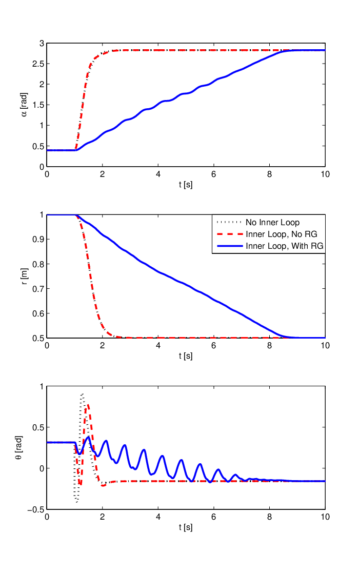
Refer to caption
Figure 4: System evolution during the numerical experiment.
Figure 5: Cable tension during the numerical experiment.

As illustrated in Figures 4-5, in the absence of an attitude error the system dynamics asymptotically tend to the desired setpoint and do not violate the taut cable constraint. In the presence of the inner loop, the system has a similar dynamic response. However, the presence of an attitude error causes the violation of the taut cable constraint at time t=1.5​[s]t=1.5[s]. The introduction of a Reference Governor is instead able to enforce the taut cable constraint at all times, even in the presence of a non-ideal inner loop. Although the dynamic response is slower than the previous cases, it is interesting to note that the Reference Governor has the added effect of greatly reducing the maximal cable tension that is reached during the transient.

10 CONCLUSIONS

This paper provides a novel approach for the study of tethered UAVs in the taut cable configuration. The cable tension is modeled as a reaction force caused by a mechanical constraint. The system dynamics are then obtained under the hypothesis that the taut cable condition is verified at all times. The attainable equilibrium points are discussed and interpreted geometrically. An inner/outer loop control strategy is developed with the dual objective of controlling the UAV and guaranteeing the taut cable condition. The outer loop is designed to automatically satisfy the constraints given under the assumption of an ideal inner loop. The inner loop error dynamics are then accounted for using a reference governor to avoid constraint violation. Future work will aim at the extension to the three-dimensional case as well as the investigation of a more sophisticated reference governor strategy to improve the system response.

References

  • [1] R. W. Beard, T. W. McLain, D. B. Nelson, D. Kingston, and D. Johanson. Decentralized cooperative aerial surveillance using fixed-wing miniature uavs. Proceeedings of the IEEE, 94(7):1306–1324, 2006.
  • [2] Sophie Eeckhout, Marco M. Nicotra, Roberto Naldi, and Emanuele Garone. Nonlinear control of an actuated tethered airfoil. In Mediterrenian Conference on Control and Automation (MED), June 2014.
  • [3] E. Feron and E. N. Johnson. Aerial robotics. In B. Siciliano and O. Khatib, editors, Springer Handbook of Robotics, pages 1009–1027. Springer, 2008.
  • [4] Minh-Duc Hua, Tarek Hamel, Pascal Morin, and Claude Samson. Introduction to feedback control of underactuated VTOL vehicles. IEEE Control Systems Magazine(CSM), 33(1):61–75, 2013.
  • [5] Alberto Isidori. Nonlinear Control Systems II. Springer, 1995.
  • [6] Ilya Kolmanovsky, Emanuele Garone, and Stefano Di Cairano. Command governors: A tutorial on their theory and automotive applications. In Invited Tutorial at ACC 2014, Submitted, 2014.
  • [7] Sergei Lupashin and Raffaello D’Andrea. Stabilization of a flying vehicle on a taut tether using inertial sensing. In IEEE/RSJ International Conference on Intelligent Robots and Systems (IROS), Nov. 2013.
  • [8] Lorenzo Marconi and Alberto Isidori. Robust global stabilization of a class of uncertain feedforward nonlinear systems. Systems and Control Letters, 41(4):281–290, 2000.
  • [9] Lorenzo Marconi and Roberto Naldi. Control of aerial robots. hybrid force/position feedback for a ducted-fan. IEEE Control Systems Magazine, 32(4):43–65, 2012.
  • [10] D. Mellinger, M. Shomin, N. Michael, and V. Kumar. Cooperative grasping and transport using multiple quadrotors. Distributed Autonomous Robotic Systems, 83:545–558, 2013.
  • [11] Frédéric Muttin. Umbilical deployment modeling for tethered UAV detecting oil pollution from ship. Journal of Applied Ocean Research, 33(4):332–343, 2011.
  • [12] Roberto Naldi, Michele Furci, Riccardo G. Sanfelice, and Lorenzo Marconi. Global trajectory tracking for underactuated VTOL aerial vehicles using cascade control paradigms. In IEEE Conference on Decision and Control (CDC), Dec. 2013.
  • [13] Roberto Naldi, Andrea Gasparri, and Emanuele Garone. Cooperative pose stabilization of an aerial vehicle through physical interaction with a team of ground robots. In IEEE International Conference on Control Applications (CCA), 2012.
  • [14] Marco M. Nicotra, Roberto Naldi, and Emanuele Garone. Taut cable control of a tethered UAV. In International Federation of Automatic Control (IFAC) World Congress, Aug. 2014.
  • [15] So-Ryeok Oh, Kaustubh Pathak, Sunil K. Agrawal, Hemanshu Roy Pota, and Matt Garratt. Approaches for a tether-guided landing of an autonomous helicopter. IEEE Transactions on Robotics, 22(3):536–544, 2006.
  • [16] Paul E. I. Pounds, Daniel R. Bersak, and Aaron M. Dollar. Grasping from the air: Hovering capture and load stability. In IEEE International Conference on Robotics and Automation (ICRA), May 2011.
  • [17] D.C. Rye. Longitudinal stability of a hovering, tethered rotorcraft. Journal of Guidance, Control, and Dynamics, 8(6):743–752, 1985.
  • [18] Luis A. Sandino, Manuel Bejar, Konstantin Kondak, and Anibal Ollero. On the use of tethered configurations for augmenting hovering stability in small-size autonomous helicopters. Journal of Intelligent & Robotic Systems, 70(1):509–525, 2013.
  • [19] G. Schmidt and R. Swik. Automatic hover control of an unmanned tethered rotorplatform. Automatica, 10(4):393–403, 1974.
  • [20] Eduardo D. Sontag and Y. Wang. On characterizations of the input-to-state stability property. System and Control Letters, 24:351–359, 1995.
  • [21] M. Tognon and A. Franchi. Nonlinear observer-based tracking control of link stress and elevation for a tethered aerial robot using inertial-only measurements. In IEEE International Conference on Robotics and Automation (ICRA), 2015.
  • [22] J. Willmann, F. Augugliaro, T. Cadalbert, R. D’Andrea, F. Gramazio, and M. Kohler. Aerial robotic construction towards a new field of architectural research. International Journal of Architectural Computing, 10(3):439–460, 2012.

.1 Proof of Proposition 11

For the sake of simplicity, the upper and lower bound of r⁡(t)r\left(t\right) will be proven only for the case r⁡(0)≥r¯r\left(0\right)\geq\bar{r}.
The initial conditions for the system are divided in four possible cases:
1- 0<r˙​(τ1)≤λ1/kD​r0<\dot{r}\left(\tau_{1}\right)\leq\lambda_{1}/k_{Dr}. Let τ1\tau_{1} and τ2\tau_{2} be such that r˙​(t)<0\dot{r}\left(t\right)<0, ∀t∈[τ1,τ2)\forall t\in\left[\tau_{1},\tau_{2}\right). In this time period, it follows that

r¨=−σλ1​(kD​r​r˙+σλ2​(kP​r​(r−r¯)))≤−σλ1​(kD​r​r˙).\ddot{r}\!=\!-\sigma_{\lambda_{1}}\left(k_{Dr}\dot{r}\!+\!\sigma_{\lambda_{2}}\left(k_{Pr}\left(r-\bar{r}\right)\right)\right)\leq-\sigma_{\lambda_{1}}\left(k_{Dr}\dot{r}\right). (45)

Thus implying that the trajectories of (45) can be upper-bounded by the solution of r¨=−kD​r​r˙\ddot{r}=-k_{Dr}\dot{r}. Therefore, conditions

r˙​(t)≤r˙​(τ1)​e−kD​r​t≤r˙​(τ1),\dot{r}\left(t\right)\leq\dot{r}\left(\tau_{1}\right)\mathrm{e}^{-k_{Dr}t}\leq\dot{r}\left(\tau_{1}\right),
r⁡(t)≤r⁡(τ1)+1kD​r​r˙​(τ1)​(1−e−kD​r​t)≤r⁡(τ1)+r˙​(τ1)kD​rr\left(t\right)\leq r\left(\tau_{1}\right)+\frac{1}{k_{Dr}}\dot{r}\left(\tau_{1}\right)\left(1-\mathrm{e}^{-k_{Dr}t}\right)\leq r\left(\tau_{1}\right)+\frac{\dot{r}\left(\tau_{1}\right)}{k_{Dr}}

and

r⁡(τ1)≤r⁡(t)r\left(\tau_{1}\right)\leq r\left(t\right)

hold true ∀t∈[τ1,τ2)\forall t\in\left[\tau_{1},\tau_{2}\right).
Due to the presence of the term −σλ2​(kP​r​(r−r¯))-\sigma_{\lambda_{2}}(k_{Pr}\left(r-\bar{r}\right)), there exists a finite time τ2\tau_{2} at which r˙​(τ2)=0\dot{r}\left(\tau_{2}\right)=0. At this time instant, future trajectories can be studied by re-initializing the system in cases 2 or 3.
2- −λ1/kD​r≤r˙(τ2)≤0-\lambda_{1}/k_{Dr}\leq\dot{r}\left(\tau_{2}\right)\leq 0 and r⁡(τ2)−r¯>λ2/kP​rr(\tau_{2})-\bar{r}>\lambda_{2}/k_{Pr}. Let τ2\tau_{2} and τ3\tau_{3} be such that r˙​(t)<0\dot{r}\left(t\right)<0 and r⁡(t)−r¯>λ2/kP​rr(t)-\bar{r}>\lambda_{2}/k_{Pr}, ∀t∈[τ2,τ3]\forall t\in\left[\tau_{2},\tau_{3}\right]. In this time period,

r¨=−σλ1​(kD​r​r˙+λ2).\ddot{r}=-\sigma_{\lambda_{1}}\left(k_{Dr}\dot{r}+\lambda_{2}\right).

As a result, the system asymptotically tends to the condition r˙=−λ2/kD​r\dot{r}=-\lambda_{2}/k_{Dr}. Since λ2>λ1\lambda_{2}>\lambda_{1}, conditions

|r˙​(t)|≤λ2kD​r.\left|\dot{r}(t)\right|\leq\frac{\lambda_{2}}{k_{Dr}}.
r⁡(t)≤r⁡(τ2)r(t)\leq r(\tau_{2})
r⁡(t)≥r¯+λ2kP​rr(t)\geq\bar{r}+\frac{\lambda_{2}}{k_{Pr}}

hold true ∀t∈[τ2,τ3]\forall t\in\left[\tau_{2},\tau_{3}\right].
Since r˙\dot{r} asymptotically tends to a negative value, there exists a finite time τ3\tau_{3} at which r⁡(τ3)=r¯+λ2/kP​rr(\tau_{3})=\bar{r}+\lambda_{2}/k_{Pr}. At time τ3\tau_{3}, the system will always satisfy the requirements of case 3.
3- −λ2/kD​r≤r˙(τ3)≤0-\lambda_{2}/k_{Dr}\leq\dot{r}\left(\tau_{3}\right)\leq 0 and kP​r​r~​(τ3)+r˙​(τ3)≥0\sqrt{k_{Pr}}\tilde{r}(\tau_{3})+\dot{r}(\tau_{3})\geq 0. Since the saturation functions σλ​1\sigma_{\lambda 1} and σλ​2\sigma_{\lambda 2} are not active at time τ3\tau_{3}, consider the dynamics of the linear system

r¨=−kD​r​r˙−kP​r​(r−r¯)\ddot{r}=-k_{Dr}\dot{r}-k_{Pr}\left(r-\bar{r}\right)

initialized in these conditions. Following from the standard linear systems theory, for kD​r=2​kP​rk_{D}r=2\sqrt{k_{Pr}}, the trajectory satisfies

r⁡(t)=r¯+r~​(τ3)​e−kP​r​t+(kP​r​r~​(τ3)+r˙​(τ3))​t​e−kP​r​tr(t)=\bar{r}+\tilde{r}(\tau_{3})e^{-\sqrt{k_{Pr}}t}+(\sqrt{k_{Pr}}\tilde{r}(\tau_{3})+\dot{r}(\tau_{3}))te^{-\sqrt{k_{Pr}}t} (46)

for t∈[τ3,∞)t\in[\tau_{3},\infty). During this whole time period, trajectory (46) will never activate the saturation functions. By studying the local minima of equation (46), it can be shown that kP​r​r~​(τ3)+r˙​(τ3)≥0\sqrt{k_{Pr}}\tilde{r}(\tau_{3})+\dot{r}(\tau_{3})\geq 0 is a necessary and sufficient condition to ensure the absence of overshoot. As a result,

|r˙​(t)|≤r˙​(τ3)|\dot{r}(t)|\leq\dot{r}(\tau_{3})
r¯≤r⁡(t)≤r⁡(τ3)\bar{r}\leq r(t)\leq r(\tau_{3})

hold true ∀t∈[τ3,∞]\forall t\in\left[\tau_{3},\infty\right].
The final case left to consider concerns what happens when the initial conditions will lead to an overshoot.
4- −λ1/kD​r≤r˙(τ4)<0-\lambda_{1}/k_{Dr}\leq\dot{r}\left(\tau_{4}\right)<0 and kP​r​r~​(τ4)+r˙​(τ4)<0\sqrt{k_{Pr}}\tilde{r}(\tau_{4})+\dot{r}(\tau_{4})<0. As in the previous case, the system trajectory is

r⁡(t)=r¯+r~​(τ4)​e−kP​r​t+(kP​r​r~​(τ4)+r˙​(τ4))​t​e−kP​r​tr(t)=\bar{r}+\tilde{r}(\tau_{4})e^{-\sqrt{k_{Pr}}t}+(\sqrt{k_{Pr}}\tilde{r}(\tau_{4})+\dot{r}(\tau_{4}))te^{-\sqrt{k_{Pr}}t}

for t∈[τ4,∞)t\in[\tau_{4},\infty). This time, however, the system trajectory presents a local minima at time

τ∗=τ4+r˙​(τ4)kP​r​r~​(τ4)+kP​r​r˙​(τ4),\tau^{*}=\tau_{4}+\frac{\dot{r}(\tau_{4})}{k_{Pr}\tilde{r}(\tau_{4})+\sqrt{k_{Pr}}\dot{r}(\tau_{4})},

thus leading to the maximum overshoot

r∗=r¯+(r~​(τ4)+r˙​(τ4)kP​r)​e−kP​r​τ∗.r^{*}=\bar{r}+\left(\tilde{r}(\tau_{4})+\frac{\dot{r}(\tau_{4})}{\sqrt{k_{Pr}}}\right)e^{-\sqrt{k_{Pr}}\tau^{*}}.

The proof is concluded by combining the properties of all four cases and doing an analogous study for r⁡(0)<r¯r\left(0\right)<\bar{r}.

.2 Proof of Proposition 14

Define xα=[α−α¯,α˙]Tx_{\alpha}=\left[\alpha-\bar{\alpha},\dot{\alpha}\right]^{T}. The state space expression of system (30) is

{x˙α​1=xα​2x˙α​2=−fα​(xα​1,xα​2)+Γ⁡(r,r¨,α~,θ~)\left\{\begin{array}[]{l}\dot{x}_{\alpha 1}=x_{\alpha 2}\\ \dot{x}_{\alpha 2}=-f_{\alpha}\left(x_{\alpha 1},x_{\alpha 2}\right)+\Gamma\left(r,\ddot{r},\tilde{\alpha},\tilde{\theta}\right)\end{array}\right.

where

fα​(xα​1,xα​2)=(kP​α​xα​1+kD​α​xα​2)​cos⁡θ~−2​r˙r​(1−cos⁡θ~)​xα​2f_{\alpha}\!\left(x_{\alpha 1},x_{\alpha 2}\right)\!=\!\left(k_{P\alpha}x_{\alpha 1}+k_{D\alpha}x_{\alpha 2}\right)\!\cos\tilde{\theta}-2\frac{\dot{r}}{r}\!\left(1-\cos\tilde{\theta}\right)\!x_{\alpha 2}

represents the state-dependent dynamics whereas

Γ⁡(r,r¨,α~,θ~)=gr​(cos⁡θ~−1)​cos⁡(α~+α¯)−uTm​r​sin⁡θ~.\Gamma\left(r,\ddot{r},\tilde{\alpha},\tilde{\theta}\right)=\frac{g}{r}\left(\cos\tilde{\theta}-1\right)\cos\left(\tilde{\alpha}+\bar{\alpha}\right)-\frac{u_{T}}{mr}\sin\tilde{\theta}.

can be seen as an exogenous bounded input since |cos⁡(α~+α¯)|≤1\left|\cos\left(\tilde{\alpha}+\bar{\alpha}\right)\right|\leq 1. To prove ISS, the first step will be the identification of a strict Lyapunov function in the condition Γ=0\Gamma=0. To this end, define kP​α=ωα2k_{P\alpha}=\omega_{\alpha}^{2} kD​α=2​ζ​ωαk_{D\alpha}=2\zeta\omega_{\alpha} and consider the Candidate Lyapunov function

V=12​xαT​[hp+q​hdqq1]​xαV=\frac{1}{2}x_{\alpha}^{T}\left[\begin{array}[]{cc}h_{p}+qh_{d}&q\\ q&1\end{array}\right]x_{\alpha}

where hp=ωα2​θ~maxh_{p}=\omega_{\alpha}^{2}\tilde{\theta}_{\max}, hd=2​ζ​ωα​θ~maxh_{d}=2\zeta\omega_{\alpha}\tilde{\theta}_{\max} and q∈(0,hd)q\in\left(0,h_{d}\right). The time derivative is

V˙=−q​ωα2​cos⁡θ~​xα​12−2​(ζ​ωα​cos⁡θ~+r˙r​(1−cos⁡θ~)−q)​xα​22+((ωα2+2​q​ζ​ωα)​(θ~max−cos⁡θ~)+2​q​r˙r​(−cos⁡θ~))​xα​1​xα​2\begin{array}[]{l}\dot{V}=\!-q\omega_{\alpha}^{2}\cos\tilde{\theta}x_{\alpha 1}^{2}-\!2\left(\zeta\omega_{\alpha}\cos\tilde{\theta}+\frac{\dot{r}}{r}\left(1-\cos\tilde{\theta}\right)\!-q\right)\!x_{\alpha 2}^{2}\\ +\!\left(\!\left(\omega_{\alpha}^{2}+2q\zeta\omega_{\alpha}\right)\!\left(\!\tilde{\theta}_{\max}\!\!-\cos\tilde{\theta}\right)\!+\!2q\frac{\dot{r}}{r}\left(\!1\!-\!\cos\tilde{\theta}\right)\!\right)\!x_{\alpha 1}x_{\alpha 2}\end{array}

which is upper-bounded by

V˙≤xαT​Q​xα\dot{V}\leq x_{\alpha}^{T}Qx_{\alpha}

where

Q=[Q11Q12Q12Q22]Q=\left[\begin{array}[]{cc}Q_{11}&Q_{12}\\ Q_{12}&Q_{22}\end{array}\right]

and

Q11=q​ωα2​θ~maxQ12=12​(ωα2+2​q​(ζ​ωα−‖r˙r‖∞))​(1−θ~max)Q22=2​ζ​ωα​θ~max−2​‖r˙r‖∞​(1−θ~max)−q\begin{array}[]{l}Q_{11}=q\omega_{\alpha}^{2}\tilde{\theta}_{\max}\\ Q_{12}=\frac{1}{2}\left(\omega_{\alpha}^{2}+2q\left(\zeta\omega_{\alpha}-\left\|\frac{\dot{r}}{r}\right\|_{\infty}\right)\right)\left(1-\tilde{\theta}_{\max}\right)\\ Q_{22}=2\zeta\omega_{\alpha}\tilde{\theta}_{\max}-2\left\|\frac{\dot{r}}{r}\right\|_{\infty}\left(1-\tilde{\theta}_{\max}\right)-q\end{array}

As a result, it follows that Q<0⇒V˙<0Q<0\Rightarrow\dot{V}<0. To obtain a negative-definite QQ it is necessary to impose q>0q>0 and ensure

q​ωα2​θ~max​(2​ζ​ωα​θ~max−2​‖r˙r‖∞​(−θ~max)−q)>14​(ωα2+2​q​(ζ​ωα−‖r˙r‖∞))2​(1−θ~max)2.\begin{array}[]{l}q\omega_{\alpha}^{2}\tilde{\theta}_{\max}\!\!\left(2\zeta\omega_{\alpha}\tilde{\theta}_{\max}\!\!\!-\!2\left\|\frac{\dot{r}}{r}\right\|_{\infty}\!\!\left(1\!-\!\tilde{\theta}_{\max}\right)\!-\!q\right)\\ >\frac{1}{4}\left(\omega_{\alpha}^{2}+2q\left(\zeta\omega_{\alpha}-\left\|\frac{\dot{r}}{r}\right\|_{\infty}\right)\right)^{2}\left(1-\tilde{\theta}_{\max}\right)^{2}.\end{array} (47)

By parameterizing

‖r˙r‖∞=ν​ζ​ωα​θ~max(1−θ~max)\left\|\frac{\dot{r}}{r}\right\|_{\infty}=\nu\frac{\zeta\omega_{\alpha}\tilde{\theta}_{\max}}{\left(1-\tilde{\theta}_{\max}\right)} (48)

with ν∈(0,1)\nu\in\left(0,1\right), equality (47) becomes

q​ωα2​θ~max​(2​ζ​ωα​θ~max​(1−ν)−q)>14​(ωα2+2​q​ζ​ωα​(1−ν))2​(1−θ~max)2.\begin{array}[]{l}q\omega_{\alpha}^{2}\tilde{\theta}_{\max}\left(2\zeta\omega_{\alpha}\tilde{\theta}_{\max}\left(1-\nu\right)-q\right)\\ >\frac{1}{4}\left(\omega_{\alpha}^{2}+2q\zeta\omega_{\alpha}\left(1-\nu\right)\right)^{2}\left(1-\tilde{\theta}_{\max}\right)^{2}.\end{array}

At this point, the parameter q∈(0,hd)q\in(0,h_{d}) can be chosen so as to maximise the term to the left of the inequality. Thus, by choosing

q=ζ​ωα​θ~max​(1−ν)q=\zeta\omega_{\alpha}\tilde{\theta}_{\max}\left(1-\nu\right)

equality (47) becomes

a​ωα4​θ~max3>b​ωα4​(1−θ~max)2a\omega_{\alpha}^{4}\tilde{\theta}_{\max}^{3}>b\omega_{\alpha}^{4}\left(1-\tilde{\theta}_{\max}\right)^{2}

with

a=(1−ν)2​ζ2b=14​(1+2​(1−ν)2​ζ2)2.\begin{array}[]{l}a=\left(1-\nu\right)^{2}\zeta^{2}\\ b=\frac{1}{4}\left(1+2\left(1-\nu\right)^{2}\zeta^{2}\right)^{2}.\end{array}

At this point, the value of ‖θ~‖∞\left\|\tilde{\theta}\right\|_{\infty} which guarantees Q<0Q<0 can then be obtained by solving

a​θ~max3−b​(1−θ~max)2>0.a\tilde{\theta}_{\max}^{3}-b\left(1-\tilde{\theta}_{\max}\right)^{2}>0. (49)

Having obtained a negative definite V˙\dot{V}, consider what happens if Γ≠0\Gamma\neq 0. Following the same reasoning as before, the derivative of V⁡(xα)V(x_{\alpha}) is lower bounded by

V˙≤−xαT​Q​xα+xαT​R​Γ\dot{V}\leq-x_{\alpha}^{T}Qx_{\alpha}+x_{\alpha}^{T}R\Gamma

where

R=[q1].R=\left[\begin{array}[]{c}q\\ 1\end{array}\right].

To prove ISS, it is sufficient to note that

xαT​R​Γ≤‖xα‖​‖R​Γ‖x_{\alpha}^{T}R\Gamma\leq\left\|x_{\alpha}\right\|\left\|R\Gamma\right\|

and

xαT​Q​xα≥λ¯Q​‖xα‖2x_{\alpha}^{T}Qx_{\alpha}\geq\underline{\lambda}_{Q}\left\|x_{\alpha}\right\|^{2}

where λ¯Q\underline{\lambda}_{Q} is the lowest eigenvalue of the positive definite matrix QQ. As a result,

‖xα‖≥‖R​Γ‖\left\|x_{\alpha}\right\|\geq\left\|R\Gamma\right\|

implies V˙≤0\dot{V}\leq 0, thus proving ISS whenever θ~\tilde{\theta} and r˙/r\dot{r}/r satisfy inequalities (48)-(49).

.3 Proof of Proposition 15

Define xθ=[θ~,θ˙]Tx_{\theta}=\left[\tilde{\theta},\dot{\theta}\right]^{T} and q=kP​θq=\sqrt{k_{P\theta}}. The closed loop dynamics of the inner loop are

x˙θ=[01−q2−2​ζ​q]​xθ+[10]​θ˙Cθ~=[10]​xθ.\begin{array}[]{l}\dot{x}_{\theta}=\left[\begin{array}[]{cc}0&1\\ -q^{2}&-2\zeta q\end{array}\right]x_{\theta}+\left[\begin{array}[]{c}1\\ 0\end{array}\right]\dot{\theta}_{C}\\ \;\;\tilde{\theta}=\left[\begin{array}[]{cc}1&0\end{array}\right]x_{\theta}\end{array}. (50)

Since the state matrix is Hurwitz, the system is ISS [20]. The asymptotic gain γIn\gamma_{\mathrm{In}} between the input θ˙C\dot{\theta}_{C} and the output θ~\tilde{\theta} is the ℓ1\ell_{1} norm

γIn=∫0∞|C​eA​s​B|​𝑑s\gamma_{\mathrm{In}}=\int_{0}^{\infty}\left|Ce^{As}B\right|\mathrm{d}s (51)

Given ζ∈(0,1)\zeta\in\left(0,1\right), the two eigenvalues of the state matrix AA are complex-conjugate. The matrix exponential can therefore be re-written as

eA​t=(2​Σ​cos⁡ω​t−2​Ω​sin⁡ω​t)​eσ​t,e^{At}=\left(2\Sigma\cos\omega t-2\Omega\sin\omega t\right)e^{\sigma t},

where

σ=Re⁡(λ1)ω=Im⁡(λ1)Σ=Re⁡(v1​w1T)Ω=Im⁡(v1​w1T)\begin{array}[]{ll}\sigma=\mathrm{Re}\left(\lambda_{1}\right)&\omega=\mathrm{Im}\left(\lambda_{1}\right)\\ \Sigma=\mathrm{Re}\left(v_{1}w_{1}^{T}\right)&\Omega=\mathrm{Im}\left(v_{1}w_{1}^{T}\right)\end{array}

and λ1\lambda_{1} is the first eigenvalue of the state matrix whereas v1v_{1} and w1w_{1} are the corresponding left and right eigenvectors. As a result,

eA​t=([1001]​cos⁡ω​t+11−ζ2​[−ζ−1qqζ]​sin⁡ω​t)​e−q​ζ​te^{At}=\left(\!\left[\!\begin{array}[]{cc}1&0\\ 0&1\end{array}\!\right]\!\cos\omega t+\frac{1}{\sqrt{1-\zeta^{2}}}\!\left[\!\begin{array}[]{cc}-\zeta&-\frac{1}{q}\\ q&\zeta\end{array}\!\right]\!\sin\omega t\!\right)\!e^{-q\zeta t}

and

C​eA​s​B=(cos⁡ω​t−ζ1−ζ2​sin⁡ω​t)​e−q​ζ​t.Ce^{As}B=\left(\cos\omega t-\frac{\zeta}{\sqrt{1-\zeta^{2}}}\sin\omega t\right)e^{-q\zeta t}. (52)

By combining (51)-(52), it follows that

γIn=∫0∞|cos⁡(ω​s)−ζ1−ζ2​sin⁡(ω​s)|​e−q​ζ​s​𝑑s.\gamma_{\mathrm{In}}=\int_{0}^{\infty}\left|\cos(\omega s)-\frac{\zeta}{\sqrt{1-\zeta^{2}}}\sin(\omega s)\right|e^{-q\zeta s}\mathrm{d}s.

For any ζ∈(0,1)\zeta\in(0,1), the following upper bound applies

γIn≤1ζ​q.\gamma_{\mathrm{In}}\leq\frac{1}{\zeta q}.